Moderation

Paul Jose

PSYC 325

Thought for the day:

“All things in moderation”

What is it?

• What is the definition of moderation?– “A moderating variable is a third

variable that affects the relationship between two others, so that the nature of the impact of the predictor on the criterion varies according to the level or value of the moderator” (Holmbeck, 1997, p. 599).

• Hmm. Nice definition, but what does it mean in the real world with real variables?

• I think that learning about moderation is helped by learning what mediation is at the same time. So what’s mediation?

Mediation

• “A mediating variable is one which specifies how (or the mechanism by which) a given effect occurs” between an independent variable (IV) and a dependent variable (DV). (Holmbeck, 1997, p. 599).

• Okay, is that clear? Well, maybe not perfectly. Let’s delve into these two phenomena more deeply, and hopefully at the end of my explanation it will be clearer.

My definitions• Moderation: this tells you the

circumstances under which the main effect occurs. If you don’t obtain a significant moderation effect, then you know that the main effect applies about equally at all levels of the IV and moderator. If you do obtain a significant moderation, then you need to look at a figure to see under what joint conditions of the moderator and IV the main effect occurs.

• Mediation: this tells you about the “mechanism” of how the IV affects the DV. Does the effect of the IV “go through” the mediator, or does it merely have a simple direct effect?

• Let’s look at some diagrams.

Stress Outcome

Stress

Coping

Mediation

Moderation

Outcome

Coping

Statistically, how are they different or similar?

• Let’s begin with moderation.• Let’s choose an IV (e.g., stress), and

a potential moderating variable (e.g., coping), as predictors of a DV (e.g., depression).

• Aiken & West recommend that you centre these two main effects, i.e., subtract the mean from the variables. Reduces multicollinearity. Not a z-score.

• Then you create a product term by multiplying the two main effects. (What do you do when you have a categorical moderator like gender? I’ll show you later.)

• Then you regress your DV on your IVs in a hierarchical fashion.

I’ve always been dubious about this centering thing—

does it matter?

Correlations

1 .481** .929**

. .000 .000

2060 2018 2030

.481** 1 .678**

.000 . .000

2018 2031 2018

.929** .678** 1

.000 .000 .

2030 2018 2030

Pearson Correlation

Sig. (2-tailed)

N

Pearson Correlation

Sig. (2-tailed)

N

Pearson Correlation

Sig. (2-tailed)

N

EMUCH

RUMINATE

product w/o centering

EMUCH RUMINATEproduct w/ocentering

Correlation is significant at the 0.01 level (2-tailed).**.

Uncentred variables

Okay, this is with centering

Correlations

1 .481** .317**

. .000 .000

2031 2018 2018

.481** 1 .408**

.000 . .000

2018 2060 2018

.317** .408** 1

.000 .000 .

2018 2018 2018

Pearson Correlation

Sig. (2-tailed)

N

Pearson Correlation

Sig. (2-tailed)

N

Pearson Correlation

Sig. (2-tailed)

N

rumination centered

emuch centered

product w/ centering

ruminationcentered

emuchcentered

product w/centering

Correlation is significant at the 0.01 level (2-tailed).**.

Alright, it does seem to make a difference! So don’tforget to center first.

The centering controversy

• I just said that one should centre one’s variables before creating the product term.

• Why? I have read that centering them prevents multicolliearity (and my correlations support this contention).

• I have never actually tested this hypothesis with regard to graphing the results, so I decided to do so.

• I used the centered and uncentered stress and rumination scores in separate regressions, and I found the following:

Results• No differences in beta weights,

significances, or R2s for the main effects.

• No difference in significances or R2s on the third step,

• But the beta weights were different on the third step.

• Why? It has to do with this issue of correlations among the three predictors.

• Is this a reason to be concerned? Only if you report and use the beta weights.

• Most important question: do these two methods yield different figures? Answer: no. See the following pages.

Uncentered variables

-2.00

-1.50

-1.00

-0.50

0.00

0.50

1.00

1.50

2.00

low med high

Stress

Rumination

high

med

low

Centered variables

-2.00

-1.50

-1.00

-0.50

0.00

0.50

1.00

1.50

2.00

low med high

Stress

Rumination

high

med

low

So what to do?

• I don’t think that it’s a major issue. You can choose to do it or not as you wish, and it won’t affect the important outcomes: significances, R2s, or the resulting figures.

• Purists will require it, but this is because they hand-computed means for figures. We don’t have to do that anymore.

• So don’t sweat it.

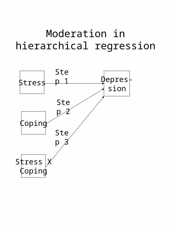
Moderation in hierarchical regression

Stress

Coping

Stress XCoping

Depres-sion

Step 1

Step 2

Step 3

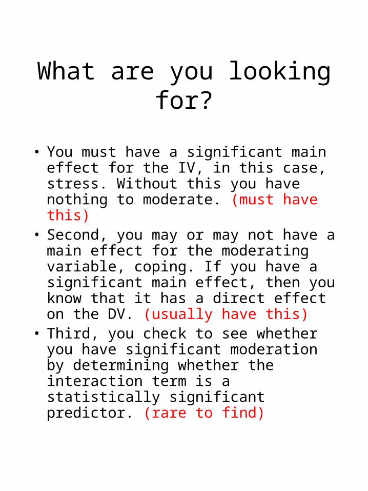
What are you looking for?

• You must have a significant main effect for the IV, in this case, stress. Without this you have nothing to moderate. (must have this)

• Second, you may or may not have a main effect for the moderating variable, coping. If you have a significant main effect, then you know that it has a direct effect on the DV. (usually have this)

• Third, you check to see whether you have significant moderation by determining whether the interaction term is a statistically significant predictor. (rare to find)

Let’s look at the SPSS print-out

Coefficientsa

-5.26E-03 .040 -.133 .895

7.096E-02 .003 .541 26.827 .000

-1.18E-02 .037 -.323 .747

4.788E-02 .003 .365 17.093 .000

9.630E-02 .006 .363 16.992 .000

4.249E-02 .039 1.077 .282

5.123E-02 .003 .391 17.445 .000

9.937E-02 .006 .375 17.407 .000

-1.03E-03 .000 -.076 -3.672 .000

(Constant)

emuch centered

(Constant)

emuch centered

rumination centered

(Constant)

emuch centered

rumination centered

product w/ centering

Model1

2

3

B Std. Error

UnstandardizedCoefficients

Beta

StandardizedCoefficients

t Sig.

Dependent Variable: NEGADJa.

Interpretation please . . .

• Stress (emuch: how much stress is caused by everyday life events) is a main effect predictor, = .54, R2 = .29, p < .001. More stress, worse negative adjustment.

• Rumination (amount of thinking about one’s negative affect) is a positive and significant predictor, = .36, R2 change = .10, p < .001. More rumination, worse negative adjustment.

• Stress by rumination (product term) is a negative and significant predictor, = -.08, R2 change = .005, p < .001. What does this mean? Notice the small unique variance. Huge sample (N = 2,500).

The magic of ModGraphTM

• Let me now introduce you to ModGraph, and tell you what it can do. Since I’m inordinately proud of it, I can’t help but show it off.

• The point I’d like to make from the previous page is: “one cannot interpret the interaction from a significant beta weight”. One must graph the interaction to learn what it means.

• How does one graph these? Well, one could laboriously hand-compute 9 algebraic formulae, and then either draw a figure or import the means for PowerPoint, or . . .

• The enlightened researcher could employ ModGraph to do this in a fraction of the time.

Moderation by Rumination

-2.00

-1.50

-1.00

-0.50

0.00

0.50

1.00

1.50

2.00

low med high

Stress

Rumination

high

med

low

The interpretation of moderation

• There are a multitude of patterns that will yield a statistically significant interaction. (I am in the process of trying to catalogue all of them.)

• Generally one looks for the “spread” or “fan” effect. The means for the three rumination groups are most different under the condition of low stress. Thus, the most easily understandable interpretation is something like,– “rumination worsens the impact of

stress on negative adjustment under conditions of low stress”.

• Notice that the spread is not dramatic; the huge sample size allowed us to find this subtle effect.

Okay, smartypants, what about categorical moderators?

• The previous example (i.e., rumination) featured a continuous moderator, but what about categorical variables like ethnic group, gender, religion, etc.?

• Well, what do you know, ModGraph can handle them too! At this time, only two-level variables can be probed. In the future, we will be able to handle n-level cases.

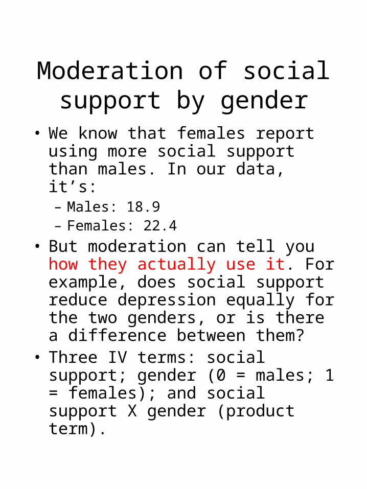
Moderation of social support by gender

• We know that females report using more social support than males. In our data, it’s:– Males: 18.9– Females: 22.4

• But moderation can tell you how they actually use it. For example, does social support reduce depression equally for the two genders, or is there a difference between them?

• Three IV terms: social support; gender (0 = males; 1 = females); and social support X gender (product term).

By the way . . .

• You can perform an ANOVA that is similar to this regression:– Neg adj as the DV; and– Gender and Social Support are the two

IVs.

• Difference? All IVs in ANOVAs must be categorical (which is fine for gender), so you must dichotomize (high vs. low) or trichotomize (high, medium, and low) social support.

• I trichotomized in this case, and see what the print-out shows.

Two main effects and an interaction:

ANOVA results

Tests of Between-Subjects Effects

Dependent Variable: CDI

4668.055a 5 933.611 16.273 .000

194493.468 1 194493.468 3390.102 .000

2048.343 2 1024.172 17.852 .000

2586.202 1 2586.202 45.079 .000

533.947 2 266.974 4.653 .010

108144.298 1885 57.371

335136.000 1891

112812.353 1890

SourceCorrected Model

Intercept

SOCTRI

GENDER

SOCTRI * GENDER

Error

Total

Corrected Total

Type III Sumof Squares df Mean Square F Sig.

R Squared = .041 (Adjusted R Squared = .039)a.

Same basic findings in the regression format

Coefficientsa

10.878 .176 61.660 .000

-.174 .032 -.126 -5.505 .000

9.315 .287 32.494 .000

-.241 .033 -.174 -7.361 .000

2.573 .375 .162 6.870 .000

9.494 .299 31.780 .000

-.145 .056 -.105 -2.609 .009

2.469 .377 .156 6.544 .000

-.145 .069 -.082 -2.112 .035

(Constant)

social sup centered

(Constant)

social sup centered

Are you male or female?

(Constant)

social sup centered

Are you male or female?

SOCXGEN

Model1

2

3

B Std. Error

UnstandardizedCoefficients

Beta

StandardizedCoefficients

t Sig.

Dependent Variable: CDIa.

The resulting figure

Moderation by Gender

-0.4

-0.3

-0.2

-0.1

0

0.1

0.2

0.3

0.4

low med high

Social support

Gender

females

males

Simple slopes

• Now there is another great feature of ModGraph that we can talk about! It has the ability to compute simple slopes, and tell you whether a particular slope is significantly different from zero.

• You need to obtain four more bits of information:– Variance of social support (SS);– Variance of the interaction (gender by

SS)– Covariance of interaction by SS; and– N of sample.

• You must request SPSS to output the covariance matrix to get the first three items. Not hard to do.

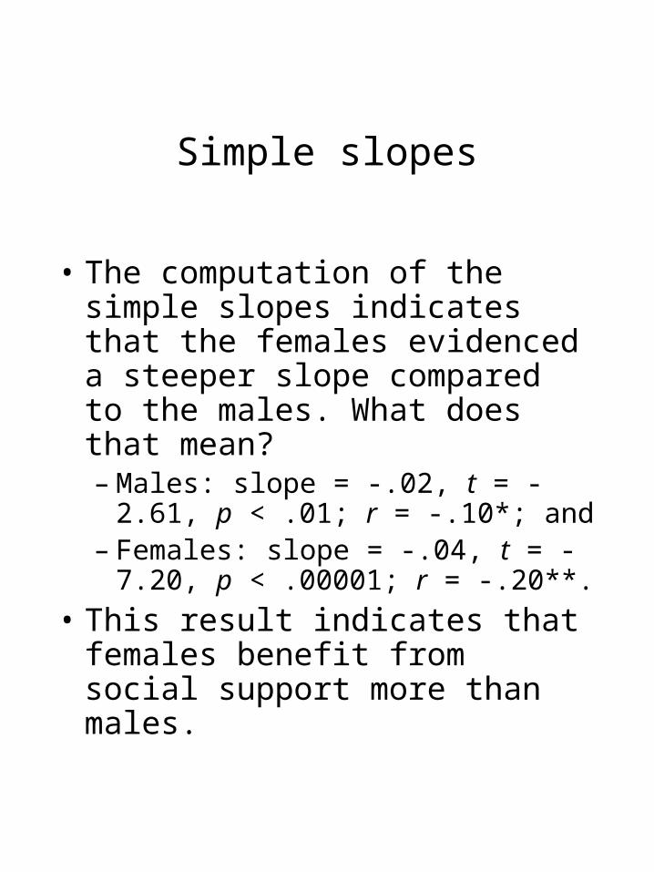
Simple slopes

• The computation of the simple slopes indicates that the females evidenced a steeper slope compared to the males. What does that mean?– Males: slope = -.02, t = -2.61, p

< .01; r = -.10*; and– Females: slope = -.04, t = -7.20, p

< .00001; r = -.20**.

• This result indicates that females benefit from social support more than males.

Okay, so what did we learn here?

(Well, besides the fact that ModGraph is just about the coolest programme this side of Doom . . ?)

• We learned:– That moderation tells you under what

circumstances something has an effect, i.e., it qualifies the main effects.

– That one cannot explain the moderation effect until you have looked at the graph.

– That interpreting interactions is difficult. Practice, practice, practice.