Modern Applied Statistics with S-PlusBenny Yakir

Abstract

These notes are based on the book Modern Applied Statistics withS-Plus by W.N. Venables and B.D. Ripley. No originality is claimed.

**************************************************** ****************************************************

Contents

1 Starting R 41.1 Installing R . . . . . . . . . . . . . . . . . . . . . . . . . . . . 41.2 Basic R Commands . . . . . . . . . . . . . . . . . . . . . . . 41.3 An Example of an R Session . . . . . . . . . . . . . . . . . . 4

2 Objects in R 62.1 Vectors and matrices . . . . . . . . . . . . . . . . . . . . . . . 62.2 Lists . . . . . . . . . . . . . . . . . . . . . . . . . . . . . . . . 72.3 Factors . . . . . . . . . . . . . . . . . . . . . . . . . . . . . . 82.4 Data frames . . . . . . . . . . . . . . . . . . . . . . . . . . . . 82.5 Homework . . . . . . . . . . . . . . . . . . . . . . . . . . . . . 8

3 Functions 103.1 Built-in functions . . . . . . . . . . . . . . . . . . . . . . . . . 103.2 Writing functions . . . . . . . . . . . . . . . . . . . . . . . . . 113.3 Plotting functions . . . . . . . . . . . . . . . . . . . . . . . . 133.4 Home Work . . . . . . . . . . . . . . . . . . . . . . . . . . . . 13

4 Linear models 144.1 A simple regression example . . . . . . . . . . . . . . . . . . 144.2 Model formulae . . . . . . . . . . . . . . . . . . . . . . . . . . 144.3 Diagnostics . . . . . . . . . . . . . . . . . . . . . . . . . . . . 164.4 Model selection . . . . . . . . . . . . . . . . . . . . . . . . . . 174.5 Homework . . . . . . . . . . . . . . . . . . . . . . . . . . . . . 18

1

5 Generalized Linear Models (GLM) 195.1 The basic model . . . . . . . . . . . . . . . . . . . . . . . . . 195.2 Analysis of deviance . . . . . . . . . . . . . . . . . . . . . . . 205.3 Fitting the model . . . . . . . . . . . . . . . . . . . . . . . . . 215.4 Generic functions and method functions . . . . . . . . . . . . 215.5 A small Binomial example . . . . . . . . . . . . . . . . . . . . 215.6 Fitting other families . . . . . . . . . . . . . . . . . . . . . . . 235.7 Frames . . . . . . . . . . . . . . . . . . . . . . . . . . . . . . . 235.8 A Poisson example . . . . . . . . . . . . . . . . . . . . . . . . 235.9 Home Work . . . . . . . . . . . . . . . . . . . . . . . . . . . . 24

6 Robust methods 266.1 Introduction . . . . . . . . . . . . . . . . . . . . . . . . . . . . 266.2 The lqs function for resistant regression . . . . . . . . . . . 266.3 Some examples . . . . . . . . . . . . . . . . . . . . . . . . . . 286.4 Home work . . . . . . . . . . . . . . . . . . . . . . . . . . . . 31

7 Non-linear Regression 337.1 The basic model . . . . . . . . . . . . . . . . . . . . . . . . . 337.2 A small example . . . . . . . . . . . . . . . . . . . . . . . . . 337.3 Attributes . . . . . . . . . . . . . . . . . . . . . . . . . . . . . 357.4 Prediction . . . . . . . . . . . . . . . . . . . . . . . . . . . . . 357.5 Profiles . . . . . . . . . . . . . . . . . . . . . . . . . . . . . . 387.6 Home work . . . . . . . . . . . . . . . . . . . . . . . . . . . . 39

8 Non-parametric and semi-parametric Regression 408.1 Non-parametric smoothing . . . . . . . . . . . . . . . . . . . 408.2 The projection-pursuit model . . . . . . . . . . . . . . . . . . 418.3 A simulated example of PP-regression . . . . . . . . . . . . . 428.4 Home work . . . . . . . . . . . . . . . . . . . . . . . . . . . . 44

9 Tree-based models 459.1 An example of a regression tree . . . . . . . . . . . . . . . . 469.2 An example of a classification tree . . . . . . . . . . . . . . . 499.3 Homework . . . . . . . . . . . . . . . . . . . . . . . . . . . . . 52

10 Multivariate analysis 5310.1 Multivariate data . . . . . . . . . . . . . . . . . . . . . . . . . 5310.2 Graphical methods . . . . . . . . . . . . . . . . . . . . . . . . 5410.3 Principal components analysis . . . . . . . . . . . . . . . . . 54

2

10.4 cluster analysis . . . . . . . . . . . . . . . . . . . . . . . . . . 5510.5 Home work . . . . . . . . . . . . . . . . . . . . . . . . . . . . 5710.6 Classification . . . . . . . . . . . . . . . . . . . . . . . . . . . 5810.7 Multivariate linear models . . . . . . . . . . . . . . . . . . . . 6410.8 Canonical correlations . . . . . . . . . . . . . . . . . . . . . . 6510.9 Project 3 . . . . . . . . . . . . . . . . . . . . . . . . . . . . . 66

3

1 Starting R

1.1 Installing R

Basic information on R can be found at the URL

http://stat.auckland.ac.nz/r/r.html

Information on how to download and install R can be found in the file:

installing-R.doc

1.2 Basic R Commands

fix(f.name) edits the function f.name in an emacs window.ls() list the files in .Data.rm(filename) delete the file filename.q() quit R.

When the program is ready for your commands you will get the “>”prompt. When you push Enter , but the command is not completed yet,you will get the “+” prompt.

You can change the working directory using File → Change dir . Thecurrent environment (image) using File → Save Image . You can thenrestore the image with File → Load Image .

To get help either use Help → R language (standard) , and then typethe name of the comand/function you like to get more information on. Alter-natively, you can use Help → R language (html) , which uses an internet-style browser,

1.3 An Example of an R Session

> bpiq <- read.table("bpiq.dat", col.names=c("dep","iq","bp"))> hist(bpiq[,"iq"],xlab="IQ",main="IQ: all children")> iq.d <- bpiq[bpiq[,"dep"]=="d","iq"]> iq.nd <- bpiq[bpiq[,"dep"]=="nd","iq"]> hist(iq.d,xlab="IQ", main="IQ: d children")

4

> hist(iq.nd,xlab="IQ", main="IQ: nd children")> t.test(iq.d,iq.nd)

Welch Two Sample t-test

data: iq.d and iq.nd t = -1.6388, df = 15.491, p-value = 0.1214alternative hypothesis: true difference in means is not equal to 095 percent confidence interval:-26.922823 3.481156

sample estimates: mean of x mean of y101.0667 112.7875

> t.test(iq.d,iq.nd, var.equal=T)

Two Sample t-test

data: iq.d and iq.nd t = -2.4801, df = 93, p-value = 0.01494alternative hypothesis: true difference in means is not equal to 095 percent confidence interval:-21.105819 -2.335847

sample estimates: mean of x mean of y101.0667 112.7875

> q()

5

2 Objects in R

2.1 Vectors and matrices

Objects are identified in S-Plus by their attributes.

> mydata <- c(2.9, 3.4, 3.4, 3.7)> colour <- c("red", "green", "blue")> x1 <- 25:30> length(mydata)[1] 4> mode(mydata)[1] "numeric"> mode(x1)[1] "numeric"> colour[2:3][1] "green" "blue"> x1[-1][1] 26 27 28 29 30> colour != "green"[1] TRUE FALSE TRUE> colour[colour != "green"][1] "red" "blue"> names(mydata) <- c(’a’, ’b’, ’c’, ’d’)> mydata

a b c d2.9 3.4 3.4 3.7

> letters[1] "a" "b" "c" "d" "e" "f" "g" "h" "i" "j" "k" "l" "m" "n" "o""p" "q" "r" [19] "s" "t" "u" "v" "w" "x" "y" "z"> mydata[letters[1:2]]

a b2.9 3.4

> matrix(x1, 2, 3)[,1] [,2] [,3]

[1,] 25 27 29[2,] 26 28 30> matrix(x1, 2, 3, byrow=T)

[,1] [,2] [,3]

6

[1,] 25 26 27[2,] 28 29 30> x2 <- matrix(x1, 2, 3)> x2[1,1][1] 25> x1 * 3[1] 75 78 81 84 87 90> x1 + x1[1] 50 52 54 56 58 60> x1 + x2

[,1] [,2] [,3][1,] 50 54 58[2,] 52 56 60> rbind(x2, x2)

[,1] [,2] [,3][1,] 25 27 29[2,] 26 28 30[3,] 25 27 29[4,] 26 28 30

2.2 Lists

Collections of other S-Plus objects.

> alist <- list(c(0,1,2), 1:10, "Name")> alist[[1]]:[1] 0 1 2

[[2]]:[1] 1 2 3 4 5 6 7 8 9 10

[[3]]:[1] "Name"

> blist <- list(x=matrix(1:10,ncol=2), y=c("A", "B"), z=alist)> blist$x

[,1] [,2][1,] 1 6

7

[2,] 2 7[3,] 3 8[4,] 4 9[5,] 5 10> blist$z[[3]][1] "Name"

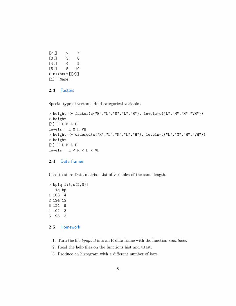
2.3 Factors

Special type of vectors. Hold categorical variables.

> height <- factor(c("H","L","M","L","H"), levels=c("L","M","H","VH"))> height[1] H L M L HLevels: L M H VH> height <- ordered(c("H","L","M","L","H"), levels=c("L","M","H","VH"))> height[1] H L M L HLevels: L < M < H < VH

2.4 Data frames

Used to store Data matrix. List of variables of the same length.

> bpiq[1:5,c(2,3)]iq bp

1 103 42 124 123 124 94 104 35 96 3

2.5 Homework

1. Turn the file bpiq.dat into an R data frame with the function read.table.

2. Read the help files on the functions hist and t.test.

3. Produce an histogram with a different number of bars.

8

4. What would happen if we would choose the argument probability=Tin the function hist?

5. Perform a one-side t.test, for α = 0.1, 0.05, 0.01.

6. Test (α = 0.05) that the mean of iq.d is 100. Repeat this analysis foriq.nd.

9

3 Functions

There are many built-in functions in S-Plus. One can write his/her ownfunctions easily. The structure of a function is:

function(arguments)expressions

3.1 Built-in functions

> data.ex <- matrix(1:50, ncol=5)> sum(data.ex)[1] 1275> mean(data.ex)[1] 25.5> var(data.ex)

[,1] [,2] [,3] [,4] [,5][1,] 9.166667 9.166667 9.166667 9.166667 9.166667[2,] 9.166667 9.166667 9.166667 9.166667 9.166667[3,] 9.166667 9.166667 9.166667 9.166667 9.166667[4,] 9.166667 9.166667 9.166667 9.166667 9.166667[5,] 9.166667 9.166667 9.166667 9.166667 9.166667> cor(data.ex)

[,1] [,2] [,3] [,4] [,5][1,] 1 1 1 1 1[2,] 1 1 1 1 1[3,] 1 1 1 1 1[4,] 1 1 1 1 1[5,] 1 1 1 1 1> apply(data.ex,2,mean)[1] 5.5 15.5 25.5 35.5 45.5> apply(data.ex,1,sum)[1] 105 110 115 120 125 130 135 140 145 150

> max(data.ex)[1] 50> min(data.ex)[1] 1> range(data.ex)

10

[1] 1 50

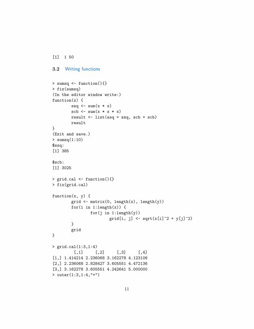
3.2 Writing functions

> sumsq <- function(){}> fix(sumsq)(In the editor window write:)function(x) {

ssq <- sum(x * x)scb <- sum(x * x * x)result <- list(ssq = ssq, scb = scb)result

}(Exit and save.)> sumsq(1:10)$ssq:[1] 385

$scb:[1] 3025

> grid.cal <- function(){}> fix(grid.cal)

function(x, y) {grid <- matrix(0, length(x), length(y))for(i in 1:length(x)) {

for(j in 1:length(y))grid[i, j] <- sqrt(x[i]^2 + y[j]^2)

}grid

}

> grid.cal(1:3,1:4)[,1] [,2] [,3] [,4]

[1,] 1.414214 2.236068 3.162278 4.123106[2,] 2.236068 2.828427 3.605551 4.472136[3,] 3.162278 3.605551 4.242641 5.000000> outer(1:3,1:4,"+")

11

[,1] [,2] [,3] [,4][1,] 2 3 4 5[2,] 3 4 5 6[3,] 4 5 6 7> h.dist <- function(x,y) sqrt(x^2 + y^2)> outer(1:3,1:4,h.dist)

[,1] [,2] [,3] [,4][1,] 1.414214 2.236068 3.162278 4.123106[2,] 2.236068 2.828427 3.605551 4.472136[3,] 3.162278 3.605551 4.242641 5.000000> system.time(grid.cal(1:100,1:100))[1] NA NA 2.46 NA NA> system.time(grid.cal(1:500,1:500))[1] NA NA 61.41 NA NA> system.time(outer(1:100,1:100,h.dist))[1] NA NA 0.04 NA NA> system.time(outer(1:500,1:500,h.dist))Error: heap memory (6144 Kb) exhausted [needed 1953 Kb more]

See "help(Memory)" on how to increase the heap size.Timing stopped at: NA NA 0.53 NA NA

> sumpow <- function(){}> fix(sumpow)

function(x, pow = 2:3){

l <- length(pow)result <- vector("list", length = l)for(i in 1:l)

result[[i]] <- sum(x^pow[i])result

}

> sumpow(1:10)[[1]]:[1] 385

[[2]]:[1] 3025

12

> sumpow(1:3,c(3,5,6))[[1]]:[1] 36

[[2]]:[1] 276

[[3]]:[1] 794

3.3 Plotting functions

The R environment provides comprehensive graphical facilities: Many higher-level plotting functions which are controlled by a verity of parameters andlower-level plotting functions which can be used in order to add to existingplots.

> x <- rnorm(10)> y <- rnorm(10)> l <- paste("(x",1:10,",y",1:10,")", sep="")> plot(x,y)> text(x,y,l)> title("Ten points")

3.4 Home Work

1. Write a function that calculates central moments of a vector.2. Read the help file on the function tapply.3. Use the function tapply to calculate the first 4 central moments of the

nd and d children iq and bp.4. Write a function that returns the indices of elements of a vector which

are more then 2 std from the vector mean.5. Identify the children which are more than 2 std from the mean

(a) in the full list.(b) within each subgroup.

6. Write a function that produces a bubble plot, i.e. given 3 vectors x, yand r it plots circles of radius r, centered at (x, y). (Use the functionsymbols.) Generate 3 random vectors of length 20 and try the function.

13

4 Linear models

4.1 A simple regression example

Linear models are the core of classical statistics: Regression, ANOVA, Anal-ysis of covariance and much more. R’S basic fitting function is lm (and aovfor ANOVA). Here we consider a simple case of linear regression.

> trees.dat <- read.table("trees.dat", col.names=c("Diameter",+ "Height", "Volume"))> attach(trees.dat)> trees.fit <- lm(Volume ~ Diameter + Height)> summary(trees.fit)

Call: lm(formula = Volume ~ Diameter + Height)

Residuals:Min 1Q Median 3Q Max

-6.4065 -2.6493 -0.2876 2.2003 8.4847

Coefficients:Estimate Std. Error t value Pr(>t)

(Intercept) -57.9877 8.6382 -6.713 2.75e-07 *** Diameter4.7082 0.2643 17.816 < 2e-16 *** Height 0.3393 0.13022.607 0.0145 *---Signif. codes: 0 ‘***’ 0.001 ‘**’ 0.01 ‘*’ 0.05 ‘.’0.1‘’1

Residual standard error: 3.882 on 28 degrees of freedom MultipleR-Squared: 0.948, Adjusted R-squared: 0.9442 F-statistic: 255on 2 and 28 degrees of freedom, p-value: 0

4.2 Model formulae

The basic formula for a linear model is:

Y = β′X + ε,

14

where Y is a random vector (or matrix), X is a design matrix of knownconstants, β is an unknown vector of parameters and ε is a random vector.

For example, for multiple regression with three explanatory variables themodel

Y = β0 + β1x1 + β2x2 + β3x3 + ε

is specified by the formula

y ˜ x1 + x2 + x3

Note that

• The left hand side is a vector or a matrix.

• The intercept is implicit.

• In the right hand side vectors or matrices, separated by +.

• To remove intercept use y ˜ − 1 + x1 + x2 + x3.

Factors generate columns in X to allow separate parameters for eachlevel. Hence, if a1 and a2 are two factors then

y ˜ a1 + x1

is a model for parallel regression (analysis of covariance) and

y ˜ a1 + a2

is a two-way ANOVA, with no interaction. To get the model with interactionuse

y ˜ a1 + a2 + a1 : a2,

ory ˜ a1 ∗ a2.

The nested model

y = β0 + αa1 + βa1x1 + ε

is formulated by y ˜ a1+a1 : x1, whereas the formula y ˜ a1∗x1 correspondsto

y = β0 + αa1 + β1x1 + βa1x1 + ε

Terms like a1 ∗ a2 ∗ a3 would generate the model

a1 + a2 + a3 + a1 : a2 + a1 : a3 + a2 : a3 + a1 : a2 : a3,

15

and terms like (a1 + a2 + a3)ˆ2 correspond to

a1 + a2 + a3 + a1 : a2 + a1 : a3 + a2 : a3.

To allow operators to be used with their arithmetic meaning use the I(·)function. For example

profit ^ I(dollar.inc + 1.55*pound.inc)

To fit polynomials use the function poly, hence

y ~ poly(x1, x2, 3)

corresponds to orthogonal polynomials of degree 3 in x1 and x2.

4.3 Diagnostics

The basic tool for examining the fit is the residuals. They are not indepen-dent.

var(e) = σ2[I −H],

where H = X(X ′X)−1X ′ is the hat matrix and e is the vector of residuals. Ifthe leverage hii of the observation is large (more than 3 or 2 times p/n, wherep is the number of explanatory variables and n the number of observations)than the observation is influential.

The standardized residuals

e′ =e

s√

1− h

or the jackknifed residuals

e∗ =y − y(·)

var(y − y(·))= e′

/[n− p− e′2

n− p− 1

]1/2

are used to examine normality and identify outlayers with the normal or half-normal probability plot. The residual plot is used to identify non-randompatterns.

> trees.res <- residuals(trees.fit)> trees.prd <- predict(trees.fit)> s <- summary(trees.fit)$sigma> h <- lm.influence(trees.fit)$hat> trees.res <- trees.res/(s*sqrt(1-h))

16

> par(mfrow=c(2,1))> plot(trees.dat[,"Diameter"],trees.res, xlab="Diameter",+ ylab="Std. Residuals")> abline(h=0, lty=2)> title("Std. Residuals vs. Diameter")> plot(trees.dat[,"Height"],trees.res, xlab="Height",+ ylab="Std. Residuals")> abline(h=0, lty=2)> title("Std. Residuals vs. Height")> par(mfrow=c(1,1))> plot(trees.prd, trees.res, xlab="Predicted Volume",+ ylab="Std. Residuals")> abline(h=0, lty=2)> title("Std. Residuals vs. Fitted Values")> par(pty="s")> qqnorm(trees.res, ylab="Std. Residuals")> title("Normal plot of Std. Residuals")> plot(1:31, h, type="n", xlab="index",+ ylab="Diagonal of hat matrix")> abline(h=mean(h))> segments(1:31,h,1:31,mean(h))> title("Leverage measure")

4.4 Model selection

Statistical hypothesis testing is all about comparing between models.

> trees1.fit <- lm(Volume ~ Diameter + I(Diameter^2) + Height)> anova(trees1.fit,trees.fit)Analysis of Variance Table

Model 1: Volume ~ Diameter + I(Diameter^2) + Height Model 2:Volume ~ Diameter + HeightRes.Df Res.Sum Sq Df Sum Sq F value Pr(>F)

1 27 186.01 2 28 421.92 -1 -235.91 34.2433.13e-06 ***---Signif. codes: 0 ‘***’ 0.001 ‘**’ 0.01 ‘*’ 0.05 ‘.’ 0.1 ‘’ 1

17

A disadvantage of this approach that it does not take into account thecomplexity of the models. In principle, one prefers simpler models — i.e.models with less parameters. Hence, one may want to consider introducinga penalty which grows with the number of parameters which are used forthe fit. This is known as Information Criteria. Examples include:

ACI: 2[maxθ∈K `(θ)−maxθ∈H `(θ)] + 2[dim(K)− dim(H)].

BCI: 2[maxθ∈K `(θ)−maxθ∈H `(θ)] + log n[dim(K)− dim(H)].

Cp: σ−2[Sum of Squares Diff.] + 2[dim(K)− dim(H)].

Given a nested sequence H ⊂ K1 ⊂ K2 ⊂ · · · ⊂ KJ the model with thesmallest information criteria should be preferred

4.5 Homework

1. The data frame cars.dat gives the speed of cars and the distances takento stop. Note that the data were recorded in the 1920s. It contains 50observations on 2 variable:speed: (numeric) Speed (mph).dist: (numeric) Stopping distance (ft).

Analyze the relation between these two variables.2. The data frame cereales.dat gives the calories, fat and fiber content of

different types of cereals. It contains 77 observations on 3 variable:cal: (numeric) Calories.fat: (numeric) Total fat.fiber: (factor) Fibers.

Analyze the calories as a function of total fat and the fiber content.

18

5 Generalized Linear Models (GLM)

5.1 The basic model

GLM extends linear models to accommodate both non-normal response andtransformations to linearity. Assumptions:

• The distribution of Yi is of the form:

fθi(yi) = exp[Ai{yiθi − γ(θi)}/ψ + τ(yi, ψ/Ai)],

where ψ is a (nuisance) scale parameter, Ai known weights. The distri-bution is controlled by the θis

• The mean of Y , µ, is a function of a linear combination of the predictors:

µ = m(β′x) = l−1(β′x).

l is called the link function. If l = (γ′)−1 then θ = β′x and l is called thecanonical link function.

Examples:

Normal: log f(y) = {yµ− µ2/2}/σ2 − 12{y

2/σ2 + log[2πσ2]}.

θ = µ

γ(θ) = θ2/2(µ) = µ

lψ = σ2.

Poisson: log f(y) = y logµ− µ− log(y!).

θ = log µγ(θ) = eθ

µ = eθ

l(µ) = log(µ)ψ = 1.

19

Binomial: Y = k/n. log f(y) = n[y log p

1−p + log(1− p)]

+ log

(nny

).

γ(θ) = log(1 + eθ

)µ = eθ/

(1 + eθ

)l(µ) = log(µ/(1− µ))ψ = 1A = n.

The parameters are estimated using MLE. The maximum is calculatedusing iterative regression.

5.2 Analysis of deviance

The parameters in the saturated model S are not constrained. The mean ofthe ith observation is estimated by the observation itself. The deviance ofthe model M , M ⊂ S, is:

DM = 2n∑i=1

Ai[{yiθS − γ(θS)

}−{yiθM − γ(θM )

}].

This is the unscaled generalized log-likelihood-ratio statistic.In the Gaussian family

DM/ψ ∼ χ2n−p,

hence ψ = DM/(n− p) is unbiased. In some other cases these relations maybe approximately true or not true at all.

When ψ is known, testing the fit of the model M relative to the nullmodel M0, where M0 ⊂ M , is performed with chi-square test of (DM0 −DM )/ψ. When ψ is unknown, testing is performed with a F test of (DM0 −DM )/(ψ(p− q)).

An alternative approach is to apply the AIC criteria, where

AIC = DM + 2pψ

(ψ should be the same across all models.)

20

5.3 Fitting the model

The basic fitting function is glm, for which the basic arguments are

glm(formula, family, data, weights, control)

formula: of the linear predictor.

family: gives the family name with additional information. For example:

function = binomial(link=probit)

fits a binomial response with the probit link.

control: of the iterative process. For example maxit determines the maxi-mal number of iterations.

5.4 Generic functions and method functions

R functions are designed to be as general as possible. The function summary,for example, can be used on many objects. This is achieved by a constructionwhich includes a generic function which is associated with method functions.A method function performs the appropriate operation on an object of aspecific class. For example, summary.glm produces a summary of objects ofclass glm. Each object has among its attributes a vector class, which is usedby the generic function in order to call the appropriate method function.

Generic functions with methods for glm include coef, resid, print, sum-mary, anova, predict, deviance.

5.5 A small Binomial example

> options(contrast=c("contr.treatment", "contr.poly"))> ldose <- rep(0:5, 2)> numdead <- c(1,4,9,13,18,20,0,2,6,10,12,16)> sex <- factor(rep(c("M","F"), c(6,6)))> SF <- cbind(numdead, numalive=20-numdead)> budworm.fit <- glm(SF ~ sex*ldose, family=binomial)> summary(budworm.fit)

21

Call: glm(formula = SF ~ sex * ldose, family = binomial)

Deviance Residuals:Min 1Q Median 3Q Max

-1.39849 -0.32094 -0.07592 0.38220 1.10375

Coefficients:Estimate Std. Error z value Pr(>z)

(Intercept) -2.9935 0.5525 -5.418 6.02e-08 *** sex0.1750 0.7781 0.225 0.822 ldose 0.9060 0.16715.424 5.84e-08 *** sex.ldose 0.3529 0.2699 1.3070.191---Signif. codes: 0 ‘***’ 0.001 ‘**’ 0.01 ‘*’ 0.05 ‘.’ 0.1 ‘ ’ 1

(Dispersion parameter for binomial family taken to be 1)

Null deviance: 124.8756 on 11 degrees of freedomResidual deviance: 4.9937 on 8 degrees of freedom AIC: 43.104

Number of Fisher Scoring iterations: 3

> plot(c(1,32), c(0,1), type="n", xlab="dose", ylab="prob", log="x")> text(2^ldose, numdead/20, as.character(sex))> ld <-seq(0, 5, 0.1)> lines(2^ld, predict(budworm.fit, data.frame(ldose=ld,+ sex=factor(rep("M", length(ld)), levels=levels(sex))),+ type="response"))> lines(2^ld, predict(budworm.fit, data.frame(ldose=ld,+ sex=factor(rep("F", length(ld)), levels=levels(sex))),+ type="response"))> anova(update(budworm.fit, . ~ sex + ldose + factor(ldose)), test="Chisq")Analysis of Deviance Table

Model: binomial, link: logit

Response: SF

Terms added sequentially (first to last)

22

Df Deviance Resid. Df Resid. Dev P(>Chi)NULL 11 124.876sex 1 6.077 10 118.799 0.014ldose 1 112.042 9 6.757 0.000factor(ldose) 4 1.744 5 5.013 0.783

5.6 Fitting other families

The families of distribution available for glm are the gaussian, binomial,poisson, inverse.gaussian and gamma. Other families can be defined.

The function make.family can be used with arguments:

name: The name of the family.

link: A list with the link function, its inverse, and its derivative.

variance: A list with the variance and deviance functions.

5.7 Frames

An evaluation frame is a list that associates names with values. The frameof the session is frame 0. Any expression evaluated in the interactive levelis evaluated in frame 1. Frames are added as evaluations become morecomplex. A name is searched for in the local frame. If it is not there thesearch moves to frame 1, then to frame 0 and then through the search path.

5.8 A Poisson example

> quine.dat <- read.table("quine.dat",header=T)> attach(quine.dat)> glm(Days ~.^4, family=poisson, data = quine.dat)

Call: glm(formula = Days ~ .^4, family = poisson, data = quine.dat)

Coefficients:(Intercept) Eth Sex AgeF1

3.0564 -0.1386 -0.4914 -0.6227

23

AgeF2 AgeF3 Lrn Eth.Sex-2.3632 -0.3784 -1.9577 -0.7524

Eth.AgeF1 Eth.AgeF2 Eth.AgeF3 Eth.Lrn0.1029 -0.5546 0.0633 2.2588

Sex.AgeF1 Sex.AgeF2 Sex.AgeF3 Sex.Lrn0.4092 3.1098 1.1145 1.5900

AgeF1.Lrn AgeF2.Lrn AgeF3.Lrn Eth.Sex.AgeF12.6421 4.8585 NA -0.3105

Eth.Sex.AgeF2 Eth.Sex.AgeF3 Eth.Sex.Lrn Eth.AgeF1.Lrn0.3469 0.8329 -0.1639 -3.5493

Eth.AgeF2.Lrn Eth.AgeF3.Lrn Sex.AgeF1.Lrn Sex.AgeF2.Lrn-3.3315 NA -2.4285 -4.1914

Sex.AgeF3.Lrn Eth.Sex.AgeF1.Lrn Eth.Sex.AgeF2.Lrn Eth.Sex.AgeF3.LrnNA 2.1711 2.1029 NA

Degrees of Freedom: 145 Total (i.e. Null); 118 ResidualNull Deviance: 2074Residual Deviance: 1174 AIC: 1818

> days.mean <- tapply(Days, list(Eth, Sex, Age,Lrn), mean)> days.var <- tapply(Days, list(Eth, Sex, Age,Lrn), var)> days.std <- sqrt(days.var)> plot(mays.mean, days.std)

5.9 Home Work

1. Use the rep and seq functions to produce the vectors:1 2 3 4 1 2 3 4 1 2 3 4 1 2 3 44 4 4 4 3 3 3 3 2 2 2 2 1 1 1 11 2 2 3 3 3 4 4 4 4 5 5 5 5 5

2. Re-analyze thebudworm data. Replace ldose by ldose-3 and see that sexis significant. What is the predicted death rate at dose=7 (i) if the sex isunknown? (ii) if sex=“M”?

3. Write the density of negative-binomial family in the exponential-familyform. What are θ, γ(θ), ψ, A, and the canonical link function?

4. The data set quine.dat contains the outcome of an observational study onnumber of days absent from school during one year in a town in Australia.The kids are classified by four factors:

24

Eth: Ethnic group. A = aboriginal, N = non-aboriginal.

Sex: M, F.

Age: F0 = Primary, F1 = first form, F3 = second form, F4 = third form.

Lrn: AL = average learner, SL = slow learner.

Investigate this data set using glm. Identify important factors and inter-actions.

25

6 Robust methods

6.1 Introduction

Robust methods are methods which will work under a wide spectrum ofcircumstances. Two of the main aspects of robustness are:

1. Resistance to outliers. Methods with high breakdown point. The estimatesare not effected much even if the value of a large portion of the observationis given an arbitrary value.

2. Robustness to distributional assumptions. The method is still efficienteven if the distributional assumptions are violated.

The usual least squares methods are neither resistant nor robust.

6.2 The lqs function for resistant regression

Usagelqs(x, ...)lqs.formula(formula, data = NULL, ...,

method = c("lts", "lqs", "lms", "S", "model.frame"),subset, na.action = na.fail, model = TRUE,x = FALSE, y = FALSE, contrasts = NULL)

lqs.default(x, y, intercept, method = c("lts", "lqs", "lms", "S"),quantile, control = lqs.control(...), k0 = 1.548, seed, ...)

lmsreg(...)ltsreg(...)print.lqs(x, digits, ...)residuals.lqs(x)

Argumentsformula a formula of the form y ~ x1 + x2 + ...{}{}.data data frame from which variables specified in formula are

preferentially to be taken.subset An index vector specifying the cases to be used in fitting.

(NOTE: If given, this argument must be named exactly.)na.action A function to specify the action to be taken if NAs are

found. The default action is for the procedure to fail.

26

An alternative is na.omit, which leads to omission of caseswith missing values on any required variable. (NOTE: Ifgiven, this argument must be named exactly.)

x a matrix or data frame containing the explanatory variables.y the response: a vector of length the number of rows of x.intercept should the model include an intercept?method the method to be used. model.frame returns the model frame:

for the others see the Details section. Using lmsreg or ltsregforces "lms" and "lts" respectively.

quantile the quantile to be used: see Details. This is over-ridden ifmethod = "lms".

control additional control items: see Details.seed the seed to be used for random sampling: see .Random.seed. The

current value of .Random.seed will be preserved if it is set..... arguments to be passed to lqs.default or lqs.control.

DescriptionFit a regression to the good points in the dataset, thereby achievinga regression estimator with a high breakdown point. lmsreg and ltsregare compatibility wrappers.

DetailsSuppose there are n data points and p regressors, including any intercept.The first three methods minimize some function of the sorted squaredresiduals. For methods "lqs" and "lms" is the quantile squared residual,and for "lts" it is the sum of the quantile smallest squared residuals."lqs" and "lms" differ in the defaults for quantile, which arefloor((n+p+1)/2) and floor((n+1)/2) respectively. For "lts" the defaultis ‘floor(n/2) + floor((p+1)/2)’.

The "S" estimation method solves for the scale s such that the average ofa function chi of the residuals divided by s is equal to a given constant.

The control argument is a list with components item{psamp}{ the size ofeach sample. Defaults to p. } item{nsamp}{ the number of samples or "best"or "exact" or "sample". If "sample" the number chosen is min(5*p, 3000),taken from Rousseeuw and Hubert (1997). If "best" exhaustive enumerationis done up to 5000 samples: if "exact" exhaustive enumeration will beattempted however many samples are needed. } item{adjust}{ should theintercept be optimized for each sample? }

27

ValueAn object of class "lqs".

NOTEThere seems no reason other than historical to use the lms and lqs options.LMS estimation is of low efficiency (converging at rate n^{-1/3}) whereasLTS has the same asymptotic efficiency as an M estimator with trimming atthe quartiles (Marazzi, 1993, p.201). LQS and LTS have the same maximalbreakdown value of (floor((n-p)/2) + 1)/n attained iffloor((n+p)/2) <= quantile <= floor((n+p+1)/2). The only drawback mentionedof LTS is greater computation, as a sort was thought to be required(Marazzi, 1993, p.201) but this is not true as a partial sort can be used(and is used in this implementation).Adjusting the intercept for each trial fit does need the residuals to besorted, and may be significant extra computation if n is large and p small.

Opinions differ over the choice of psamp. Rousseeuw and Hubert (1997) onlyconsider p; Marazzi (1993) recommends p+1 and suggests that more samplesare better than adjustment for a given computational limit.

The computations are exact for a model with just an intercept andadjustment, and for LQS for a model with an intercept plus one regressorand exhaustive search with adjustment. For all other cases the minimizationis only known to be approximate.

6.3 Some examples

Let us compare the two of the robust methods, lms and lts with the usuallm.

> .Random.seed <- 1:4> library(lqs)> x30 <- runif(30, 0.5, 4.5)> e30 <- rnorm(30, 0, 0.2)> y30 <- 2+ x30+ e30> x20 <- runif(20, 5, 7)> y20 <- rnorm(20, 2, 0.5)> y <- c(y30, y20)

28

> x <- c(x30, x20)> plot(x,y)> abline(lm(y~x), lty=1)> abline(lmsreg(x,y), lty=2)> abline(ltsreg(x,y), lty=3)> legend(4.5,6, legend=c("LS","LMS","LTS"), lty=1:3)

Figure 1: Plot of lm, lms and lts

29

Consider next the internal dataset stackloss obtained from 21 days ofoperation of a plant for the oxidation of ammonia (NH3) to nitric acid(HNO3). The nitric oxides produced are absorbed in a countercurrent ab-sorption tower.

x1: represents the rate of operation of the plant.

x2: is the temperature of cooling water circulated through coils in the ab-sorption tower.

x3: is the concentration of the acid circulating, minus 50, times 10: that is,89 corresponds to 58.9 per cent acid.

y: (the dependent variable) is 10 times the percentage of the ingoing am-monia to the plant that escapes from the absorption column unabsorbed;that is, an (inverse) measure of the over-all efficiency of the plant.

> data(stackloss)> stack.lm <- lm(stack.loss ~ stack.x)> summary(stack.lm)

Call:lm(formula = stack.loss ~ stack.x)

Residuals:Min 1Q Median 3Q Max

-7.2377 -1.7117 -0.4551 2.3614 5.6978

Coefficients:Estimate Std. Error t value Pr(>t)

(Intercept) -39.9197 11.8960 -3.356 0.00375 **stack.xAir.Flow 0.7156 0.1349 5.307 5.8e-05 ***stack.xWater.Temp 1.2953 0.3680 3.520 0.00263 **stack.xAcid.Conc. -0.1521 0.1563 -0.973 0.34405---Signif. codes: 0 ‘***’ 0.001 ‘**’ 0.01 ‘*’ 0.05 ‘.’ 0.1 ‘ ’ 1

Residual standard error: 3.243 on 17 degrees of freedomMultiple R-Squared: 0.9136, Adjusted R-squared: 0.8983F-statistic: 59.9 on 3 and 17 degrees of freedom, p-value: 3.016e-009

30

> stack.lts <- ltsreg(stack.x, stack.loss)> stack.lms <- lmsreg(stack.x, stack.loss)> stack.lm$coef(Intercept) stack.xAir.Flow stack.xWater.Temp stack.xAcid.Conc.-39.9196744 0.7156402 1.2952861 -0.1521225

> stack.lts$coef(Intercept) Air.Flow Water.Temp Acid.Conc.-3.630556e+01 7.291667e-01 4.166667e-01 6.336445e-16

> stack.lms$coef(Intercept) Air.Flow Water.Temp Acid.Conc.-3.425000e+01 7.142857e-01 3.571429e-01 -2.791275e-16

> par(mfrow=c(2,2))> plot(fitted(stack.lm),resid(stack.lm))> abline(h=0)> title("LS regression")> plot(fitted(stack.lts),resid(stack.lts))> abline(h=0)> title("LTS regression")> plot(fitted(stack.lms),resid(stack.lms))> abline(h=0)> title("LMS regression")

6.4 Home work

Investigate the data set hills.dat. The 3 vriables in the data set are:

dist: The overall race distance.

climb: The total height climbed.

time: The record time.

Identify outliers using the robust methods presented in class. Try themodel where observations are weighted by 1/dist2.

31

Figure 2: Plot of stackloss

32

7 Non-linear Regression

7.1 The basic model

The Basic model is:Y = f(X,β) + ε,

where Y is the response, f is a function of a known form, X are the covari-ates, β is a vector of unknown parameters and ε is the random noise. Thestructure of f is determined on scientific ground — modeling of the physicalphenomenon.

The parameters are estimated by minimizing an objective function suchas the least-squares:

n∑i=1

(Yi − f(Xi, β))2.

(When the εi are iid normal this is the MLE.) The model is fitted with thefunction nls. The arguments are:

formula The right hand side is a regular expression.

data An optional data frame.

start A list or vector specifying the starting values for parameters. Thenames of the components specify which of the components of the expres-sion in formula are parameters.

control over the iterative procedure.

algorithm Which optimization algorithm is used.

trace Tracing information from the iterative algorithm.

7.2 A small example

> hormone.dat <- read.table("hormone.txt",col.names=c("f","b"))> hormone.dat

f b1 84.6 12.12 83.9 12.5

33

3 148.2 17.24 147.8 16.75 463.9 28.36 463.8 26.97 964.1 37.68 967.6 35.89 1926.0 38.5

10 1900.0 39.9> attach(hormone.dat)> plot(f,b)> title("Observed Values")> hormone.fit <- nls(b ~ Bmax*f/(KD + f), start=list(Bmax=40,KD=250))> summary(hormone.fit)

Formula: b ~ Bmax * f/(KD + f)

Parameters:Estimate Std. Error t value Pr(>t)

Bmax 44.378 1.129 39.31 1.93e-10 ***KD 241.688 20.946 11.54 2.89e-06 ***---Signif. codes: 0 ‘***’ 0.001 ‘**’ 0.01 ‘*’ 0.05 ‘.’ 0.1 ‘ ’ 1

Residual standard error: 1.288 on 8 degrees of freedom

Correlation of Parameter Estimates:Bmax

KD 0.8281

> plot(f,b)> Bmax.hat <- coef(hormone.fit)[1]> KD.hat <- coef(hormone.fit)[2]> f.seq <- seq(range(f)[1],range(f)[2],length=100)> b.seq <- Bmax.hat*f.seq/(KD.hat + f.seq)> lines(f.seq,b.seq)> title("Observed Values and Fitted Curve")> Bmax.val <- seq(20,60,length=30)> KD.val <- seq(50,1000,length=30)> S <- matrix(0,30,30)> for(i in 1:30){

34

+ for(j in 1:30) S[i,j] <- sum((b-Bmax.val[i]*f/+ (KD.val[j] + f))^2)}> persp(Bmax.val,KD.val, S/100, xlab="Bmax",+ ylab="KD", zlab="Objective Function/100")

A. B. C.

Figure 3: A=hormone data, B=predicted, C=objective function

7.3 Attributes

All objects in R have a mode and a length attributes. Some have otherattributes like names or dim. Attributes are handled with the functions:

attributes(x) Return or change all attributes of the object x.

attr(x, which) Returns or changes the attribute which of the object x.

dim, names ... Returns or change specific attributes.

7.4 Prediction

The data set wtloss.dat contains information on a group of male patientsthat were involved in a weight rehabilitation programme. The variables are

Days the time since the start of the programme.

35

Weight in kilograms.

The model to fit is:

W = β0 + β12−t/θ + ε.

where

β0 is the stable lean weight.

β1 is the total weight to be lost.

θ ’half life’; that time it takes to lose half of the weight.

Let η(β0, β1, θ) = β0 + β12−t/θ. Then the gradient is

∂η

∂β1= 1,

∂η

∂β2= 2−t/θ,

∂η

∂θ=

log(2)β1t2−t/θ

θ2

A crucial question is how long should one expect to be on the programmein order to achieve a particular goal weight w0. From the equation it followsthat

t0 = τ(β0, β1, θ) = −θ log2{(w0 − β0)/β1}.

Hence,t0 = −θ log2{(w0 − β0)/β1}.

Large sample (δ-method) approximation of the variance of t0 is given by

var(t0) ≈ (τ)′Στ ,

where τ is the gradient of τ and Σ is the variance-covariance matrix of theparameters estimates.

> wtloss.nls <- nls(Weight ~ b0 + b1*2^(-Days/th),+ data = wtloss.dat, start=list(b0=90,b1=95,th=120),trace = T)67.54349 : 90 95 12040.18081 : 82.72629 101.30457 138.7137439.24489 : 81.39868 102.65836 141.8586039.2447 : 81.37375 102.68417 141.91052> wtloss.eprn <- function(){}> fix(wtloss.expn)

function(b0, b1, th, t) {temp <- 2^(-t/th)

36

model.func <- b0 + b1 * tempZ <- cbind(1, temp, (b1 * t * temp * log(2))/th^2)dimnames(Z) <- list(NULL, c("b0", "b1", "th"))attr(model.func, "gradient") <- Zmodel.func

}

> wtloss1.nls <- nls(Weight ~ wtloss.expn(b0, b1, th, Days),+ data = wtloss.dat, start=list(b0=90,b1=95,th=120),trace = T)67.54349 : 90 95 12040.18081 : 82.72629 101.30457 138.7137439.24489 : 81.39868 102.65836 141.8585939.2447 : 81.37375 102.68417 141.91053> vcov <- function(fm){+ sm <- summary(fm)+ sm$cov.unscaled * sm$sigma^2}> time.pds <- deriv(~ -th * log((w0 - b0)/b1)/log(2),+ c("b0", "b1", "th"), function(w0, b0, b1, th) NULL)> est.time <- function(){}> fix(est.time)

function(w0, obj){

b <- coef(obj)tmp <- time.pds(w0, b["b0"], b["b1"], b["th"])t0 <- as.vector(tmp)dot <- attr(tmp, "gradient")v <- (dot %*% vcov(obj) * dot) %*% matrix(1,3,1)a <- cbind( t0, sqrt(v))dimnames(a) <- list(paste(w0, "kg: "), c("t0", "SE"))a

}

> est.time(c(100, 90, 85), wtloss.nls)t0 SE

100 kg: 349.4979 8.17539690 kg: 507.0941 31.21787185 kg: 684.5185 98.900230

37

7.5 Profiles

Figure 4: Profile of wtloss

The large sample derivation is based on the assumption that the log-likelihoodis (approximately) quadratic in the vicinity of the parameters true values.

38

This can be evaluated with the profile function. The profile of a parameteris the likelihood function of the given parameter, maximized with respect toall other parameters. R provides the function profile which compute thefunctions

π(βj) =sign(βj − βj)

sj

√PSS(βj)− PSS(βj).

These functions should look linear if the large sample assumptions are met.

> par(mfrow=c(2,2), pty="s")> plot(profile(wtloss.nls), ask=F)

7.6 Home work

1. Fit the model to the data set wtloss.dat using the option plinear.

2. Fit to the data both quadratic and cubic polynomials. Plot the expectedweight in the range of 0 to 700 days in the program as predicted by nls,the quadratic, and the cubic fit. Add to the plot the data points and alegend.

39

8 Non-parametric and semi-parametric Regression

8.1 Non-parametric smoothing

When the data is definitely non-linear on the one hand, and, on the otherhand, there is no scientific or empirical data to suggest another parametricstructure, non-parametric regression approaches are useful. The are usefulin data smoothing in exploratory statistics or as the non-parametric part ina semi parametric model. In the following example we examine three suchapproaches:

Kernel smoother: Is implemented by the function ksmooth. The kernelis either uniform or normal. The smoothing parameter is bandwidth.

Splines: Is implemented by the function smooth.spline. Smoothness isdetermined by the parameter spar, which is the coefficient of the integralof the squared second derivative in the penalized log likelihood criterion.Alternatively one can use df or cross validation.

Local polynomials: Is implemented by the function loess. Fitting isdone locally. That is, for the fit at point x, the fit is made using pointsin a neighborhood of x, weighted by their distance from x The size of theneighborhood is controlled by span.

> library(modreg)> data(cars)> attach(cars)> plot(speed, dist)> lines(ksmooth(speed, dist, "normal", bandwidth=2), col=2)> lines(ksmooth(speed, dist, "normal", bandwidth=5), col=3)> lines(ksmooth(speed, dist, "normal", bandwidth=10), col=4)> plot(speed, dist, main = "data(cars) & smoothing splines")> cars.spl <- smooth.spline(speed, dist)> cars.splCall:smooth.spline(x = speed, y = dist)

Smoothing Parameter (Spar): 0.7986363Equivalent Degrees of Freedom (Df): 2.520569

40

Penalized Criterion: 4380.504GCV: 244.1659> lines(cars.spl, col = "blue")> lines(smooth.spline(speed, dist, df=10), lty=2, col = "red")> legend(5,120,c(paste("default [C.V.] => df =",round(cars.spl$df,1)),+ "s( * , df = 10)"), col = c("blue","red"), lty = 1:2, bg=’bisque’)> plot(speed, dist, main = "data(cars) & loess")> lines(speed,predict(loess(dist ~ speed)),col="blue")> lines(speed,predict(loess(dist ~ speed,span=0.5)),col="red", lty=2)> legend(5,120, legend = c("default", "span=0.3"), col = c("blue","red"),+ lty = 1:2,bg=’bisque’)

8.2 The projection-pursuit model

Assume that the explanatory vector X = (X1, . . . , Xp)′ is of high dimension.In order to avoid the dimensionality problem one can fit an additive modelof the form:

Y = α0 +p∑j=1

fj(Xj) + ε.

Drawbacks of the additive model are:

1. If the dimension p is too high the additive model may be an overfit of thedata.

2. The model does not include interactions — the dependence structure inone variable depends on the level of the other variables.

An alternative is the projection-pursuit (PP) model. This model is ofthe form:

Y = α0 +M∑j=1

fj(α′jX) + ε,

where M � p, fj is smooth and αj a direction vector.The projection-pursuit model applies an additive model to projected

variables. Rather than fitting p functions in p directions the dimension canbe reduced by using only the M most significant directions. This is in thespirit of principal components. The terms are called ridge functions sincethey are constant in all but one direction.

The model is fit with the function ppr (ppreg in S-plus). Consider thefollowing example:

41

> data(rock)> attach(rock)> area1 <- area/10000; peri1 <- peri/10000> rock.ppr <- ppr(log(perm) ~ area1 + peri1 + shape,+ data = rock, nterms = 2, max.terms = 5)> summary(rock.ppr)Call:ppr.formula(formula = log(perm) ~ area1 + peri1 + shape, data = rock,

nterms = 2, max.terms = 5)

Goodness of fit:2 terms 3 terms 4 terms 5 terms

8.737806 5.289517 4.745799 4.490378

Projection direction vectors:term 1 term 2

area1 0.34357179 0.37071027peri1 -0.93781471 -0.61923542shape 0.04961846 0.69218595

Coefficients of ridge terms:term 1 term 2

1.6079271 0.5460971> par(mfrow=c(1,2), pty="s")> plot(rock.ppr, main="default")> plot(update(rock.ppr, bass=5), main = "bass=5")> plot(update(rock.ppr, sm.method="gcv", gcvpen=2), main = "gcv")

8.3 A simulated example of PP-regression

> set.seed(14)> x1 <- runif(400, -1, 1)> x2 <- runif(400, -1, 1)> eps <- rnorm(400, 0, 0.2)> y <- x1*x2 + eps> sim.pp <- ppr(y ~ x1 + x2, nterms=1, max.terms=5)> summary(sim.pp)Call:ppr.formula(formula = y ~ x1 + x2, nterms = 1, max.terms = 5)

42

Goodness of fit:1 terms 2 terms 3 terms 4 terms 5 terms

23.95768 13.51628 12.65749 11.83397 11.02952

Projection direction vectors:x1 x2

0.6411524 0.7674135

Coefficients of ridge terms:[1] 0.2651939> par(mfrow=c(3,2))> plot(x1, y, sub="Y vs X1")> plot(x2, y, sub="Y vs X2")> sim.pp <- ppr(y ~ x1 + x2, nterms=1, max.terms=5)> summary(sim.pp)Call:ppr.formula(formula = y ~ x1 + x2, nterms = 1, max.terms = 5)

Goodness of fit:1 terms 2 terms 3 terms 4 terms 5 terms

23.95768 13.51628 12.65749 11.83397 11.02952

Projection direction vectors:x1 x2

0.6411524 0.7674135

Coefficients of ridge terms:[1] 0.2651939> sim.pp2 <- ppr(y ~ x1 + x2, nterms=2)> summary(sim.pp2)Call:ppr.formula(formula = y ~ x1 + x2, nterms = 2)

Goodness of fit:2 terms

13.32762

Projection direction vectors:term 1 term 2

43

x1 0.6474445 0.5988468x2 0.7621126 -0.8008636

Coefficients of ridge terms:term 1 term 2

0.2051119 0.1749922> plot(sim.pp$fitted,sim.pp$residuals)> plot(sim.pp2$fitted,sim.pp2$residuals)> plot(sim.pp2$fitted,sim.pp$fitted)

8.4 Home work

1. Create and investigate, using ppreg, a simulated example. Try differentnumber of variables and functions thereof.

44

9 Tree-based models

A (binomial) tree is a structure which includes a root, nodes, and edges.Each node is connected by an edge to a father node and may have up totwo son nodes. The final nodes are called leaves. Each node with two sonscorresponds to a split in the data. The paths, from the root to the leaves,correspond to subsets of the data.

Tree-based modeling is a technique for:

1. Devising prediction rules that are interpretable.

2. Screening variables.

3. Assessing linear models.

4. Summarize large data sets.

We will consider tree-based classification and tree-based regression. Thedifference between the two is in the type of the response. In the later theresponse is quantitative whereas in the former it is a factor.

Regression trees can be compared to analysis of variance and/or to lmusing cut. Unlike that approach, however, the division of the range of theexplanatory variables is adaptive and it includes interactions automatically.A path is a predictor. The predicted value is attached to the leave. Sub-models correspond to sub-trees. The deviance of a model is defined as

D =n∑i=1

(Yi − Yi)2,

where Yi is the predicted value at the leave to which case i belongs.With each leave of a classification tree, a level of the response is associ-

ated. Each case which is associated with the path that leads to that leave isclassified by that level. Deviances are defined by the multinomial likelihoodof different levels. Criteria like the entropy or Gini index are used in growingthe tree.

Trees are grown until the number of cases reaching each leave is small(by default < 10) or the leave is homogeneous (by default less than 1% ofthe total deviance.) This usually leads to trees that overfit the data andpruning is needed.

Functions for fitting trees can be found in the library tree. This li-brary is not part of the basic R package. It can be downloaded from

45

http://cran.r-project.org/src/contrib/PACKAGES.html. Installing isdone with the program rwinst.exe (which was used to install the basicpackage). This program is available athttp://cran.r-project.org/bin/windows/windows-9x/base/.

9.1 An example of a regression tree

The data set cpus.dat contains information on relative performance measureand characteristics of 209 CPUs. The components are:

name Manufacturer and model.

syct cycle time in nanoseconds.

mmin minimum main memory in kilobytes.

mmax maximum main memory in kilobytes.

cach cache size in kilobytes.

chmin minimum number of channels.

chmax maximum number of channels.

perf published performance on a benchmark mix relative to an IBM370/158-3.

estperf estimated performance (by Ein-Dor & Feldmesser).

The data comes from P. Ein-Dor & J. Feldmesser (1987) Attributes of theperformance of central processing units: a relative performance predictionmodel. Comm. ACM. 30, 308-317.

> cpus.dat <- read.table("cpus.dat", header=T,sep=",")> apply(cpus.dat[,-1], 2, mean)

syct mmin mmax cach chmin203.822967 2867.980861 11796.153110 25.205742 4.698565

chmax perf estperf18.267943 105.617225 99.330144

> sqrt(apply(cpus.dat[,-1], 2, var))syct mmin mmax cach chmin

260.262926 3878.742758 11726.564377 40.628722 6.816274chmax perf estperf

46

25.997318 160.830587 154.757102> library(tree)> cpus.tr <- tree(perf ~ syct+mmin+mmax+cach+chmin+chmax, cpus.dat)> summary(cpus.tr)

Regression tree:tree(formula = perf ~ syct + mmin + mmax + cach + chmin + chmax,

data = cpus.dat)Variables actually used in tree construction:[1] "mmax" "cach" "chmax" "mmin"Number of terminal nodes: 7Residual mean deviance: 4838 = 977300 / 202Distribution of residuals:

Min. 1st Qu. Median Mean 3rd Qu. Max.-4.756e+02 -2.144e+01 -5.638e+00 -1.707e-14 1.836e+01 3.674e+02> plot(cpus.tr)> text(cpus.tr)> title("Basic regression tree for cpus.dat")> cpus.ltr <- tree(log10(perf) ~ syct + mmin + mmax + cach + chmin + chmax,+ data=cpus.dat)> summary(cpus.ltr)

Regression tree:tree(formula = log10(perf) ~ syct + mmin + mmax + cach + chmin +

chmax, data = cpus.dat)Variables actually used in tree construction:[1] "cach" "mmax" "syct" "chmin"Number of terminal nodes: 10Residual mean deviance: 0.03187 = 6.342 / 199Distribution of residuals:

Min. 1st Qu. Median Mean 3rd Qu. Max.-4.945e-01 -1.191e-01 3.571e-04 3.240e-16 1.141e-01 4.680e-01> plot(cpus.ltr, type="u")> text(cpus.ltr)> title("Regression tree for log10(perf)")> plot(prune.tree(cpus.ltr))> title("Deviance by size of cpus.ltr")> cpus.ltr1 <- prune.tree(cpus.ltr, best=8)> plot(cpus.ltr1)> text(cpus.ltr1)

47

> title("Pruned down regression tree for log10(perf)")> cpus.cv <- cv.tree(cpus.ltr,FUN=prune.tree)> plot(cpus.cv)> title("Deviance by size of cpus.cv")> cpus.ltr2 <- prune.tree(cpus.ltr, best=4)

A. B. C.

Figure 5: (A)=default tree (B)=log(perf) (C)=size vs. deviance

A. B. C.

Figure 6: (A)=pruned tree (B)=size vs. dev, CV (C)=pruned tree, CV

48

> plot(cpus.ltr2)> text(cpus.ltr2)> title("Pruned down by CV regression tree for log10(perf)")

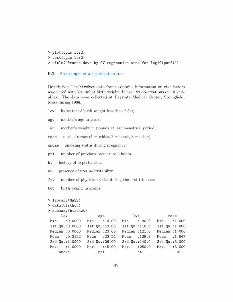
9.2 An example of a classification tree

Description The birthwt data frame contains information on risk factorsassociated with low infant birth weight. It has 189 observations on 10 vari-ables. The data were collected at Baystate Medical Center, Springfield,Mass during 1986.

low indicator of birth weight less than 2.5kg.

age mother’s age in years.

lwt mother’s weight in pounds at last menstrual period.

race mother’s race (1 = white, 2 = black, 3 = other).

smoke smoking status during pregnancy.

ptl number of previous premature labours.

ht history of hypertension.

ui presence of uterine irritability.

ftv number of physician visits during the first trimester.

bwt birth weight in grams.

> library(MASS)> data(birthwt)> summary(birthwt)

low age lwt raceMin. :0.0000 Min. :14.00 Min. : 80.0 Min. :1.0001st Qu.:0.0000 1st Qu.:19.00 1st Qu.:110.0 1st Qu.:1.000Median :0.0000 Median :23.00 Median :121.0 Median :1.000Mean :0.3122 Mean :23.24 Mean :129.8 Mean :1.8473rd Qu.:1.0000 3rd Qu.:26.00 3rd Qu.:140.0 3rd Qu.:3.000Max. :1.0000 Max. :45.00 Max. :250.0 Max. :3.000

smoke ptl ht ui

49

Min. :0.0000 Min. :0.0000 Min. :0.00000 Min. :0.00001st Qu.:0.0000 1st Qu.:0.0000 1st Qu.:0.00000 1st Qu.:0.0000Median :0.0000 Median :0.0000 Median :0.00000 Median :0.0000Mean :0.3915 Mean :0.1958 Mean :0.06349 Mean :0.14813rd Qu.:1.0000 3rd Qu.:0.0000 3rd Qu.:0.00000 3rd Qu.:0.0000Max. :1.0000 Max. :3.0000 Max. :1.00000 Max. :1.0000

ftv bwtMin. :0.0000 Min. : 7091st Qu.:0.0000 1st Qu.:2414Median :0.0000 Median :2977Mean :0.7937 Mean :29453rd Qu.:1.0000 3rd Qu.:3487Max. :6.0000 Max. :4990

> attach(birthwt)> race <- factor(race, labels=c("white","black","other"))> table(ptl)ptl0 1 2 3

159 24 5 1> ptd <- factor(ptl >0)> table(ftv)ftv0 1 2 3 4 6

100 47 30 7 4 1> ftv <- factor(ftv)> levels(ftv)[-(1:2)] <-"2+"> table(ftv)ftv0 1 2+

100 47 42> bwt <- data.frame(low=factor(low),age,lwt,race, smoke = (smoke>0),+ ptd, ht = (ht>0), ui = (ui>0), ftv)> detach(birthwt)> bwt.tr <- tree(low ~ ., bwt)> summary(bwt.tr)

Classification tree:tree(formula = low ~ ., data = bwt)Variables actually used in tree construction:[1] "ptd" "lwt" "age"

50

Number of terminal nodes: 8Residual mean deviance: 1.042 = 188.6 / 181Misclassification error rate: 0.2328 = 44 / 189> plot(bwt.tr)> text(bwt.tr)> title("Low birth weight classification tree")> bwt.tr1 <- prune.tree(bwt.tr, k=2)> summary(bwt.tr1)

Classification tree:tree(formula = low ~ ., data = bwt)Variables actually used in tree construction:[1] "ptd" "lwt" "age"Number of terminal nodes: 8Residual mean deviance: 1.042 = 188.6 / 181Misclassification error rate: 0.2328 = 44 / 189> plot(prune.tree(bwt.tr))> title("Deviance by size of bwt.tr")> plot(bwt.tr1)> text(bwt.tr1)> title("Low birth weight: bwt.tr1")

A. B. C.

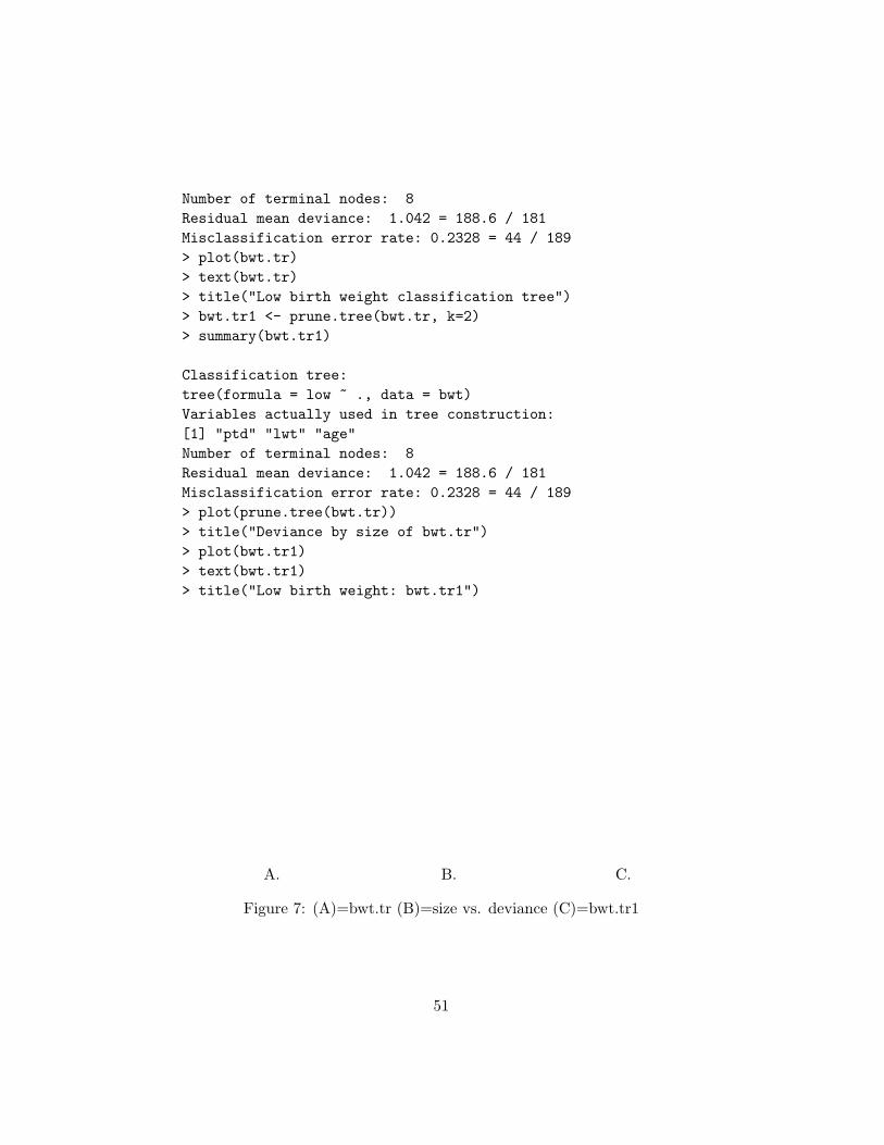
Figure 7: (A)=bwt.tr (B)=size vs. deviance (C)=bwt.tr1

51

9.3 Homework

Investigate the data set bwt using both glm and tree. Compare the results.

52

10 Multivariate analysis

10.1 Multivariate data

Multivariate analysis is concerned with datasets which have more than oneresponse variable for each observation. The dataset can be put in a matrixX with n rows and p columns.

One distinguishes between methods with a given division of the casesinto groups (supervised methods), and methods which seek to discover astructure from the data matrix alone (unsupervised methods)

The dataset we consider is the system dataset iris. This data set containsinformation on the width and length of the petals and sepals of three differentspecies of Iris: Iris setosa, Iris virginica, and Iris versicolor.

> data(iris)> summary(iris)Sepal.Length Sepal.Width Petal.Length Petal.WidthMin. :4.300 Min. :2.000 Min. :1.000 Min. :0.1001st Qu.:5.100 1st Qu.:2.800 1st Qu.:1.600 1st Qu.:0.300Median :5.800 Median :3.000 Median :4.350 Median :1.300Mean :5.843 Mean :3.057 Mean :3.758 Mean :1.1993rd Qu.:6.400 3rd Qu.:3.300 3rd Qu.:5.100 3rd Qu.:1.800Max. :7.900 Max. :4.400 Max. :6.900 Max. :2.500

Speciessetosa :50versicolor:50virginica :50

> apply(iris[,-5],2, tapply, iris[,5],mean,trim=0.1)Sepal.Length Sepal.Width Petal.Length Petal.Width

setosa 5.0025 3.4150 1.4600 0.2375versicolor 5.9375 2.7800 4.2925 1.3250virginica 6.5725 2.9625 5.5100 2.0325> apply(iris[,-5],2, tapply, iris[,5],var)

Sepal.Length Sepal.Width Petal.Length Petal.Widthsetosa 0.1242490 0.14368980 0.03015918 0.01110612versicolor 0.2664327 0.09846939 0.22081633 0.03910612virginica 0.4043429 0.10400408 0.30458776 0.07543265

53

10.2 Graphical methods

The function pairs plots an array of scatter plots. One can add labels orcolors to different observations.

> ir <- iris[,-5]> pairs(ir)> ir.species <- c(rep("s",50),rep("c",50), rep("v",50))> attributes(ir)$row.names <- ir.species> library(mva)> biplot(princomp(ir))> attributes(ir)$row.names <- 1:150

10.3 Principal components analysis

Principal components analysis seeks linear combinations of the variableswith maximal (or minimal) variance. Combinations are constraint to haveunit length.

The covariance matrix is defined by

(n− p)Σ = (X − n−11′X1)′(X − n−11′X1) = (X ′X − nxx′)

The correlation matrix can be defined in a similar way. The covariance (orcorrelation) matrix is non-negative definite hence has an eigen decomposition

Σ = C ′ΛC,

where Λ is diagonal and C ′C = I. The principle components correspond toeigenvectors of maximal eigenvalues. A measure of how good are the first kprinciple components is

k∑i=1

λi/p∑i=1

λi.

The S function prcomp works directly with X and uses the singular valuedecomposition

X = UΛV ′.

> ir.pr <- prcomp(scale(log(ir)))> plot(ir.pr$x[,1:2], type="n")> text(ir.pr$x[,1:2], ir.species)

54

> ir.pr$sdev[1] 1.7124583 0.9523797 0.3647029 0.1656840> ir.pr$rot

PC1 PC2 PC3 PC4Sepal.Length 0.5038236 -0.45499872 -0.7088547 0.19147575Sepal.Width -0.3023682 -0.88914419 0.3311628 -0.09125405Petal.Length 0.5767881 -0.03378802 0.2192793 -0.78618732Petal.Width 0.5674952 -0.03545628 0.5829003 0.58044745

10.4 cluster analysis

Cluster analysis is concerned with discovering group structure amongst thecases. A dissimilarity coefficient measures the distances between two cases.Several dissimilarity can be calculated with the function dist.

> hc <- hclust(dist(ir), "ave")> ir.species <- c(rep(".",50),rep("’",50), rep("-",50))> plot(hc, hang=-1, labels=ir.species)> title("hclust(iris), method=average")> hc <- hclust(dist(ir), "complete")> plot(hc, hang=-1, labels=ir.species)> title("hclust(iris), method=complete")> hc <- hclust(dist(ir), "single")> plot(hc, hang=-1, labels=ir.species)> title("hclust(iris), method=single")

> hc <- hclust(dist(ir), "average")> A <- list(factor(rep(cutree(hc,3), 4)),+ factor(rep(1:4,rep(dim(ir)[1],4))))> tapply(unlist(ir), A, mean)

1 2 3 41 5.006000 3.428000 1.462000 0.2460002 5.929688 2.757813 4.410938 1.4390623 6.852778 3.075000 5.786111 2.097222> initial <- tapply(unlist(ir), A, mean)> km <- kmeans(ir, initial)> km$centersSepal.Length Sepal.Width Petal.Length Petal.Width

1 5.006000 3.428000 1.462000 0.246000

55

2 5.901613 2.748387 4.393548 1.4338713 6.850000 3.073684 5.742105 2.071053> km$size[1] 50 62 38> x <- rbind(matrix(rnorm(100, sd = 0.3), ncol = 2),+ matrix(rnorm(100, mean = 1, sd = 0.3), ncol = 2))> cl <- kmeans(x, 2, 20)> plot(x, pch = cl$cluster)> points(cl$centers, col = 1:2, pch = 8)> title("A simulated example of K-means")

> library(tree)> ir.species <- factor(c(rep("s",50),rep("c",50), rep("v",50)))> ird <- data.frame(ir)> ir.tr <- tree(ir.species ~.,ird)> summary(ir.tr)Classification tree:tree(formula = ir.species ~ ., data = ird)Variables actually used in tree construction:[1] "Petal.Length" "Petal.Width" "Sepal.Length"Number of terminal nodes: 6Residual mean deviance: 0.1253 = 18.05 / 144Misclassification error rate: 0.02667 = 4 / 150

> plot(ir.tr)> text(ir.tr)> ir.tr1 <- snip.tree(ir.tr)node number: 12

tree deviance = 18.05subtree deviance = 22.77

node number: 7tree deviance = 18.05subtree deviance = 22.28

> par(pty="s")> plot(ird[,3],ird[,4], type ="n", xlab="petal length",+ ylab="petal width")> text(ird[,3],ird[,4], as.character(ir.species))> par(cex=2)> partition.tree(ir.tr1, add=T)

56

10.5 Home work

1. The system data swiss gives five measures of socio-economic data onSwiss provinces about 1888. Can you identify clusters? Use the functionkmeans.

2. Plot the data points on the principal components axis. Use the clusternumber as a mark, and add to the plot the clusters centers.

57

10.6 Classification

Modern usage of the term classification refers to allocation of future casesinto one of g classes. This is similar to discriminant analysis. This is a part ofpattern recognition, with cluster analysis is unsupervised and classification,or diagnosis is supervised.

The given cases with their classifications are a training set, and furthercases for a test set. The primary measure of success is the misclassificationrate, or error rate. A confusion matrix gives the number of cases with trueclass i classified as of class j. In some problems some errors are consideredworse than others. We will get biased estimate of success by re-classifyingthe training set.

The function lda in the MASS library creates classification rules baseon dividing the space with linear hyper-planes. Let W be the within-classcovariance matrix, and let B be the between-class covariance matrix. Let Mbe the g×d matrix of class means, and G the n×g matrix of class indicators.Then the predictions are GM . Let bx be the overall mean. Thus,

W =(X −GM)′(X −GM)

n− g, B =

(GM − 1x)′(GM − 1x)g − 1

.

Fisher’s linear discriminant rule, which is based on a linear functional, char-acterized by a vector a. The vector a maximizes the ratio a′Ba/a′Wa. Thevector a can be associated with largest eigenvalue of BW−1. Classificationis based on the level of x′a The procedure lda extends this approach byconsidering also the other eigenvalues of BW−1.

> library(MASS)> data(iris)> ir <- iris[,1:4]> ir.species <- rep(c("s","c","v"),c(50,50,50))> a<- lda(log(ir), ir.species)> a$svd^2/sum(a$svd^2)[1] 0.996498601 0.003501399> a.x <- predict(a, log(ir), dimen = 2)$x> eqscplot(a.x, type="n", xlab="first linear discriminant",+ ylab="second linear discriminat")> text(a.x, as.character(ir.species))> train <- sample(1:150, 75)> table(ir.species[train])

58

c s v29 21 25> z <- lda(ir.species ~ ., data.frame(ir,ir.species),+ prior = c(1,1,1)/3, subset = train)

Figure 8: Linear discrimination

59

> predict(z, ir[-train, ])$class[1] s s s s s s s s s s s s s s s s s s s s s s s s s s s s s c c c c c c c

[37] c c c c c v c c c c c c c c v v v v v v v v v v v v v v v v v v v v v v[73] v v vLevels: c s v

The function qda in MASS does quadratic discriminant analysis. Thiscorresponds to the Bayes rule which minimizes

L(c) = (x− xc)′W−1c (x− xc) + log(det(Wc))− 2 log πc,

where xc is the mean of class c, Wc is the estimate of the covariance matrixof the class and πc is the prior probability of belonging to the class.

> tr <- sample(1:50,25); te <- (1:50)[-tr]> train <- rbind(ir[tr,],ir[tr+50,], ir[tr+100,])> test <- rbind(ir[te,],ir[te+50,],ir[te+100,])> cl <- factor(c(rep("s",25),rep("c",25), rep("v",25)))> z <- qda(train, cl)> predict(z,test)$class[1] s s s s s s s s s s s s s s s s s s s s s s s s s c c c c c c c c c c c

[37] c c c c c c c c c c c c c c v v v v v v v v v v v v v v v v v v v v v v[73] v v vLevels: c s v

Let us compare the two procedures in the following example. The datasetCushings from the MASS package refers to some diagnostic tests on patientswith Cushing’s syndrome. Cushing’s syndrome is a hypertensive disorderassociated with over-secretion of cortisol by the adrenal gland. The obser-vations are urinary excretion rates of two steroid metabolites. There are 27observations. The variables are:

Tetrahydrocortisone: urinary excretion rate (mg/24hr) of Tetrahydro-cortisone.

Pregnanetriol: urinary excretion rate (mg/24hr) of Pregnanetriol.

Type: underlying type of syndrome, coded “a” (adenoma) , “b” (bilateralhyperplasia), “c” (carcinoma) or “u” for unknown.

(Source: J. Aitchison and I. R. Dunsmore (1975) Statistical PredictionAnalysis. Cambridge University Press, Tables 11.1-3.)

60

> predplot <- function(){}> fix(predplot)

In the editor window write:

function(object, main="", len=100, ...){

plot(Cushings[,1], Cushings[,2], type="n", log="xy",xlab="Tetrahydrocortisone", ylab="Pregnanetriol", main=main)

text(Cushings[1:21,1], Cushings[1:21,2], as.character(tp))text(Cushings[22:27,1], Cushings[22:27,2], "u")xp <- seq(0.6, 4, length = len)yp <- seq(-3.25, 2.45, length = len)cushT <- expand.grid(Tetrahydrocortisone=xp,

Pregnanetriol=yp)Z <- predict(object, cushT, ...)z <- unclass(Z$class)zp <- Z$post[,3] - pmax(Z$post[,2], Z$post[,1])contour(exp(xp), exp(yp), matrix(zp, len), add=T,levels=0, labex=0)

zp <- Z$post[,1] - pmax(Z$post[,2], Z$post[,3])contour(exp(xp), exp(yp), matrix(zp, len), add=T,levels=0, labex=0)

invisible()}

After saving and exiting:

> data(Cushings)> cush <- log(as.matrix(Cushings[,-3]))> tp <- factor(Cushings$Type[1:21])> cush.lda <- lda(cush[1:21,], tp); predplot(cush.lda, "LDA")> cush.qda <- qda(cush[1:21,], tp); predplot(cush.qda, "QDA")> predplot(cush.qda, "QDA, predictive", method="predictive")> predplot(cush.qda, "QDA, debiased", method="debiased")

(Remark: Note that you should install the latest version of R (rw1001) andthe latest version of MASS (VR.zip) on your computer. On my computerthe above examples did not work with version rw1000.)

61

A. B.

Figure 9: A= Linear, B=Quadratic

A. B.

Figure 10: A= Predictive, B=Debiased

62

The function knn in the library class (part of the base R package)performs a k-nearest neighbor classification for test set from training set.For each row of the test set, the k nearest (in Euclidean distance) trainingset vectors are found, and the classification is decided by majority vote,with ties broken at random. If there are ties for the kth nearest vector,all candidates are included in the vote. The function knn.cv in the libraryclass performs a k-nearest neighbor cross-validatory classification

> library(class)> knn(train, test,cl, k=3, prob=TRUE)[1] s s s s s s s s s s s s s s s s s s s s s s s s s c c c c c c c c c c c

[37] c v c c c v c c c c c c c c v v v v c v v v v v c v v v v v v v v v v v[73] v v vLevels: c s v> attributes(.Last.value)$levels[1] "c" "s" "v"$class[1] "factor"$prob[1] 1.0000000 1.0000000 1.0000000 1.0000000 1.0000000 1.0000000 1.0000000[8] 1.0000000 1.0000000 1.0000000 1.0000000 1.0000000 1.0000000 1.0000000

[15] 1.0000000 1.0000000 1.0000000 1.0000000 1.0000000 1.0000000 1.0000000[22] 1.0000000 1.0000000 1.0000000 1.0000000 1.0000000 1.0000000 1.0000000[29] 1.0000000 0.6666667 1.0000000 1.0000000 1.0000000 1.0000000 1.0000000[36] 1.0000000 1.0000000 0.6666667 1.0000000 1.0000000 1.0000000 0.6666667[43] 1.0000000 1.0000000 1.0000000 0.6666667 1.0000000 1.0000000 1.0000000[50] 1.0000000 1.0000000 1.0000000 1.0000000 1.0000000 1.0000000 1.0000000[57] 1.0000000 1.0000000 1.0000000 1.0000000 0.6666667 1.0000000 1.0000000[64] 1.0000000 1.0000000 0.6666667 0.6666667 1.0000000 1.0000000 0.6666667[71] 1.0000000 1.0000000 1.0000000 0.6666667 1.0000000> knn.cv(train, cl, k=3, prob=TRUE)[1] s s s s s s s s s s s s s s s s s s s s s s s s s c v c c c c c c c c c

[37] c c c c v c c c c c c c c c v c v v v v v v v v v v v v v v v v v v v c[73] v v vLevels: c s v> attributes(.Last.value)$levels[1] "c" "s" "v"$class

63

[1] "factor"$prob[1] 1.0000000 1.0000000 1.0000000 1.0000000 1.0000000 1.0000000 1.0000000[8] 1.0000000 1.0000000 1.0000000 1.0000000 1.0000000 1.0000000 1.0000000

[15] 1.0000000 1.0000000 1.0000000 1.0000000 1.0000000 1.0000000 1.0000000[22] 1.0000000 1.0000000 1.0000000 1.0000000 1.0000000 1.0000000 1.0000000[29] 1.0000000 0.7500000 1.0000000 0.6666667 1.0000000 1.0000000 0.6666667[36] 1.0000000 1.0000000 0.6666667 1.0000000 1.0000000 0.6666667 1.0000000[43] 1.0000000 1.0000000 1.0000000 1.0000000 1.0000000 1.0000000 1.0000000[50] 1.0000000 1.0000000 0.5000000 1.0000000 1.0000000 1.0000000 1.0000000[57] 0.6666667 1.0000000 0.6666667 1.0000000 1.0000000 1.0000000 1.0000000[64] 1.0000000 1.0000000 1.0000000 1.0000000 1.0000000 0.6666667 1.0000000[71] 1.0000000 0.5000000 1.0000000 0.6666667 1.0000000

10.7 Multivariate linear models

A multivariate linear model is a model of the form Y = XB+E, where Y isthe matrix of responses, X is the design matrix, B is the matrix of coefficientsand E a matrix of normally distributed errors. Parameter restrictions can beincluded by the Z matrix: ZB = 0 (which has applications in MANOVA).

Multivariate linear models can be fit with the function multilm fromthe contributed library multilm. Additionally, this function calculates theHotelling T 2-Test for the given test problem: H0 : KB = 0. An approxima-tion by Laeuter is used for the distribution of the T 2-statistic (and thereforefor the p-value).

> library(multilm)> Y <- as.matrix(iris[,1:4])> x <- c(rep(1,50), rep(0,150), rep(1, 50), rep(0, 150), rep(1,50))> X <- matrix(x, ncol=3)> Z <- c(0,1,1,1)> K <- cbind(0,diag(2),-1)> K

[,1] [,2] [,3] [,4][1,] 0 1 0 -1[2,] 0 0 1 -1> mod <- multilm(Y ~ X, K,Z)> summary(mod)test procedure: Hotelling

64

test statistic: 584.5918degrees of freedom DF1: 8 DF2: 144p-value: 0

10.8 Canonical correlations

The canonical correlation analysis seeks linear combinations of the ‘y’ vari-ables which are well explained by linear combinations of the ‘x’ variables.The relationship is symmetric as ‘well explained’ is measured by correlations.Formally, we look for vectors a and such that the correlation

corr(x′a,y′b) =a′Σxyb

(a′Σxxa)1/2(b′Σyyb)1/2

is high.The function cancor from the package mva (part of the basic installation

compute the canonical correlations between two data matrices.Here we apply it on the dataset LifeCycleSavings. Under the life-

cycle savings hypothesis as developed by Franco Modigliani, the savingsratio (aggregate personal saving divided by disposable income) is explainedby per-capita disposable income, the percentage rate of change in per-capitadisposable income, and two demographic variables: the percentage of pop-ulation less than 15 years old and the percentage of the population over 75years old. The data are averaged over the decade 1960-1970 to remove thebusiness cycle or other short-term fluctuations.

The data frame contains 50 observations on 5 variables:

sr: aggregate personal savings.

pop15: % of population under 15.

pop75: % of population over 75.

dpi: real per-capita disposable income.

ddpi: % growth rate of dpi.

> library(mva)> data(LifeCycleSavings)> pop <- LifeCycleSavings[, 2:3]> oec <- LifeCycleSavings[, -(2:3)]

65

> cancor(pop, oec)$cor[1] 0.8247966 0.3652762$xcoef

[,1] [,2][1,] -0.009110856 -0.03622206[2,] 0.048647514 -0.26031158$ycoef

[,1] [,2] [,3][1,] 0.0084710221 3.337936e-02 -5.157130e-03[2,] 0.0001307398 -7.588232e-05 4.543705e-06[3,] 0.0041706000 -1.226790e-02 5.188324e-02$xcenterpop15 pop75

35.0896 2.2930$ycenter

sr dpi ddpi9.6710 1106.7584 3.7576

> x <- matrix(rnorm(150), 50, 3)> y <- matrix(rnorm(250), 50, 5)> str(cxy <- cancor(x, y))List of 5$ cor : num [1:3] 0.3784 0.1365 0.0933$ xcoef : num [1:3, 1:3] 0.10879 -0.09125 0.06089 -0.07601 0.00771 ...$ ycoef : num [1:5, 1:5] -0.033498 0.167432 -0.022940 -0.000426 -0.077757 ...$ xcenter: num [1:3] 0.0440 -0.0723 -0.2179$ ycenter: num [1:5] -0.0121 0.1620 -0.2470 -0.0883 -0.0249

> all(abs(cor(x %*% cxy$xcoef,+ y %*% cxy$ycoef)[,1:3] - diag(cxy $ cor)) < 1e-15)[1] TRUE> all(abs(cor(x %*% cxy$xcoef) - diag(3)) < 1e-15)[1] TRUE> all(abs(cor(y %*% cxy$ycoef) - diag(5)) < 1e-15)[1] TRUE

10.9 Project 3

66

The data frame crabs in the package MASS contains morphological measure-ments on Leptograpsus crabs. This data frame has 200 rows and 8 columns,describing 5 morphological measurements on 50 crabs each of two colourforms and both sexes, of the species Leptograpsus variegatus collected atFremantle, W. Australia. The variables are:

sp: species — “B” or “O” for blue or orange.

sex: as it says.

index: index 1:50 within each of the four groups.

FL: frontal lobe size (mm).

RW: rear width (mm).

CL: carapace length (mm).

CW: carapace width (mm).

BD: body depth (mm).

Do classification analysis for this data. Create a training set and a testset. Try different approaches and compare their performance.

67