modern control systemscontrol.asu.edu/classes/mmae543/543lecture07.pdf · modern control systems...

Modern Control Systems

Matthew M. PeetIllinois Institute of Technology

Lecture 7: Controllability and Observability

State-Space

The standard state-space form is

x(t) = Ax(t) +Bu(t)

y(t) = Cx(t) +Du(t)

State-space reflects an approach based on internal dynamics as opposed toinput-output maps.

• For a given mapping, G : u 7→ y, the choice of A,B,C,D is not unique.

M. Peet Lecture 7: State-Space Theory 2 / 29

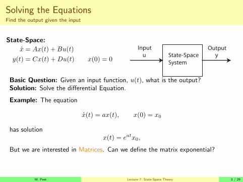
Solving the EquationsFind the output given the input

State-Space:

x = Ax(t) +Bu(t)

y(t) = Cx(t) +Du(t) x(0) = 0State-Space

System

u y

Input Output

Basic Question: Given an input function, u(t), what is the output?Solution: Solve the differential Equation.

Example: The equation

x(t) = ax(t), x(0) = x0

has solutionx(t) = eatx0,

But we are interested in Matrices. Can we define the matrix exponential?


The Solution to State-SpaceIgnore Inputs and Outputs:The equation

x(t) = Ax(t), x(0) = x0

has solution x(t) = eAtx0

The function eAt must satisfy the following

e0 = I, andd

dteAt = AeAt

For scalars, the matrix exponential is defined as

ea = 1 + a+ a2/2 + · · ·+ an

n!+ · · ·

We define the exponential for matrices is defined the same way as scalars

eA = I +A+1

2A2 +

1

6A3 + · · ·+ 1

k!Ak + · · ·


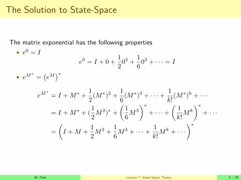
The Solution to State-Space

The matrix exponential has the following properties

• e0 = I

e0 = I + 0 +1

202 +

1

603 + · · · = I

• eM∗

=(eM)∗

eM∗

= I +M∗ +1

2(M∗)2 +

1

6(M∗)3 + · · ·+ 1

k!(M∗)k + · · ·

= I +M∗ + (1

2M2)∗ +

(1

6M3

)∗+ · · ·+

(1

k!Mk

)∗+ · · ·

=

(I +M +

1

2M2 +

1

6M3 + · · ·+ 1

k!Mk + · · ·

)∗


The Solution to State-Space

• ddte

At = AeAt

d

dteAt =

d

dt

(I + (At) +

1

2(At)2 + · · ·+ 1

k!(At)k + · · ·

)= 0 +A+

2

2A(At) +

3

6A(At)2 + · · ·+ k

k!A(At)k + · · ·

= A

(I + (At) +

1

2(At)2 + · · ·+ 1

(k − 1)!(At)k−1 + · · ·

)However,

eM+N 6= eMeN

Unless, MN = NM .


Find the output given the input

The equation x(t) = Ax(t), x(0) = x0

has solution x(t) = eAtx0

Proof.

Let x(t) = eAtx0, then

• x(t) = AeAtx0 = Ax(t).

• x(t) = e0x0 = x0

What happens when we add an input instead of an initial condition?


Find the output given the inputState-Space:

x = Ax(t) +Bu(t)

y(t) = Cx(t) +Du(t) x(0) = 0

The equation

x(t) = Ax(t) +Bu(t), x(0) = 0

has solution

x(t) =

∫ t

0

eA(t−s)Bu(s)ds

Proof.

Check the solution:

x(t) = e0Bu(t) +A

∫ t

0

eA(t−s)Bu(s)ds

= Bu(t) +Ax(t)


Find the output given the inputSolution for State-Space

State-Space:

x = Ax(t) +Bu(t)

y(t) = Cx(t) +Du(t) x(0) = 0

Now that we have x(t), finding y(t) iseasy

y(t) = Cx(t) +Du(t)

=

∫ t

0

CeA(t−s)Bu(s)ds+Du(t)

Conclusion: Given u(t), only one integration is needed to find y(t)!Note that the state, x, doesn’t appear!!

We have solved the problem.


Calculating the OutputNumerical Example, u(t) = sin(t)

State-Space:

x = −x(t) + u(t)

y(t) = x(t)− .5u(t) x(0) = 0

A = −1; B = 1; C = 1; D = −.5

Solution:

y(t) =

∫ t

0

CeA(t−s)Bu(s)ds+Du(t)

= e−t∫ t

0

es sin(s)ds− 1

2sin(t)

=1

2e−t

(es(sin s− cos s)|t0

)− 1

2sin(t)

=1

2e−t

(et(sin t− cos t) + 1

)− 1

2sin(t)

=1

2

(e−t − cos t

)

0 2 4 6 8 10−1

−0.8

−0.6

−0.4

−0.2

0

0.2

0.4

0.6

0.8

1

t

u(t)

input

0 2 4 6 8 10−0.8

−0.6

−0.4

−0.2

0

0.2

0.4

0.6

t

y(t)

output


Stability

x(t) = Ax(t)

There are several notions of stability.

• All notions are equivalent for linear systems.

Definition 1.

A differential equation is stable if any solution x(t) satisfies

limt→∞

x(t) = 0


Stability

The unique solution has the form x(t) = eAtx0.

x(t) = Ax(t)

Question: Is it stable?Suppose A is diagonalizable, so A = TΛT−1, so that

Ak = TΛT−1TΛT−1 · · ·TΛT−1 = TΛkT−1

We conclude that

eAt =

(TT−1 + (TΛT−1)t+

1

2(TΛ2T−1)t2 + · · ·+ 1

k!(TΛkT−1)tk + · · ·

)= T

(I + (Λt) +

1

2(Λt)2 + · · ·+ 1

k!(Λt)k + · · ·

)T−1

= TeΛtT−1


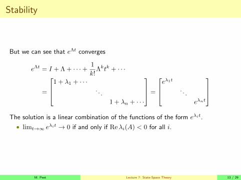
Stability

But we can see that eΛt converges

eΛt = I + Λ + · · ·+ 1

k!Λktk + · · ·

=

1 + λ1 + · · ·. . .

1 + λn + · · ·

=

eλ1t

. . .

eλnt

The solution is a linear combination of the functions of the form eλit.

• limt→∞ eλit → 0 if and only if Reλi(A) < 0 for all i.


Stability

Inconveniently, not all matrices are diagonalizable.• However, all matrices are Jordan diagonalizable.

I Ak = TJkT−1, where J

• Hence eAt = TeJtT−1

Consider a single Jordan block Ji = λiI +N .• Convenient because λiI and N commute.

I Hence eλiI+N = eλiIeN .

eJit = eλit+Nt = eλiteNt

Conveniently Nd = 0, so the series expansion terminates

eNt = 1 +N +1

2N2 + · · ·+ 1

(k − 1)!Nk−1tk−1

eJit =

eλ1t

. . .

eλnt

[1 +N +1

2N2 + · · ·+ 1

(k − 1)!Nk−1tk−1

]

This time all terms have the form tieλt for i ≤ k• limt→∞ tieλt = 0 if and only if Reλ < 0


Stability

Now consider the general case A = TJT−1 where

J =

J1

. . .

Jn

Then

eAt = TeJtT−1 = T

eJ1t

. . .

eJnt

T−1

eAt is entirely composed of terms of the form

eλittk

k!

We conclude that x(t) = Ax(t) is stable if and only if Reλ < 0.


Stability

Definition 2.

A is Hurwitz if Reλi(A) < 0 for all i.

x(t) = Ax(t) is stable if and only if A is Hurwitz.


Controllability

First add an input u(t)

x(t) = Ax(t) +Bu(t), x(0) = x0

The solution is

x(t) =

∫ t

0

eA(t−s)Bu(s)ds

Use Leibnitz rule for differentiation of integrals

x(t) = eA(t−t)Bu(t) +

∫ t

0

AeA(t−s)Bu(s)ds

= Bu(t) +Ax(t)

Controllability asks whether we can “control” the system states throughappropriate choice of u(t).

• Note that we do not care how u(t) is chosen.

We start with a weaker definition


Controllability

Definition 3.

For a given (A,B), the state xf is Reachable if for any fixed Tf , there exists au(t) such that

xf =

∫ Tf

0

eA(Tf−s)Bu(s)ds

Definition 4.

The system (A,B) is reachable if any point xf ∈ Rn is reachable.

For a fixed t, the set of reachable states is defined as

Rt := {x : x =

∫ t

0

eA(t−s)Bu(s)ds for some function u.}


Controllability

The mapping Γ : u 7→ xf is linear. Let u = αu1 + βu2

Γu =

∫ Tf

0

eA(Tf−s)B (αu1(s) + βu2(s)) ds

= α

∫ Tf

0

eA(Tf−s)Bu1(s)ds+ β

∫ Tf

0

eA(Tf−s)Bu2(s)ds

= αΓu1 + βΓu2

Thus Rt = Image(Γ).

• Rt is a subspace.

Definition 5.

For a given system (A,B), the Controllability Matrix is

C(A,B) :=[B AB A2B · · · An−1B

]where A ∈ Rn×n and B ∈ Rn×m.


Controllability

Definition 6.

For a given (A,B), the Controllable Subspace is

CAB = Image[B AB A2B · · · An−1B

]Definition 7.

The system (A,B) is controllable if

CAB = ImC(A,B) = Rn

Question: How does Rt relate to CAB?


Controllability

Definition 8.

The finite-time Controllability Grammian of pair (A,B) is

Wt :=

∫ t

0

eAsBBT eAT sds

Wt is a positive semidefinite matrix.The following relates these three concepts of controllability

Theorem 9.

For any t ≥ 0,Rt = CAB = Image (Wt)

orImage Γt = Image C(A,B) = Image (Wt)


Controllability

The most important consequence is

• Rt does not depend on time!

If you can get there, you can get there arbitrarily fast.This says nothing about how you get u(t)

• This u(t) comes from the proof (and Wt)

We can test reachability of a point x by testing

x ∈ Im[B AB A2B · · · An−1B

]The system is controllable if Wt > 0. Summary

1. Rt is the set of reachable points

2. C(A,B) is a fixed matrix, easily computable.

3. We need to find u(t)


Controllability

The following is a seminal result in state-space theory.

Theorem 10.

Ifdet(sI −A) = sn + an−1s

n−1 + · · ·+ a0

thenAn + an−1A

n−1 + an−2An−2 + · · · a0I = 0

Sketch.

The same principle as deriving the solution. Denote

charA(s) = sn + an−1sn−1 + · · ·+ a0 = det(sI −A)

Then if A = TλT−1

charA(A) = T charA(Λ)T−1 = T

charA(λ1). . .

charA(λn)

T−1


Controllability

Sketch.

But the λi are eigenvalues of A, so

charA(λ) = det(λI −A) = 0

hence

charA(A) = T

charA(λ1). . .

charA(λn)

T−1 = T

0. . .

0

T = 0

The same approach works for Jordan Blocks.

Cayley-Hamilton says

An = −an−1An−1 + · · ·+−a0I

thus An ∈ span(An−1, · · · , I)

• This is unsurprising since A has n2 dimensions but is formed by n bases.


Controllability

Proof: Show Rt ⊂ CAB for any t ≥ 0. Expand

eAt =

[I +At+ · · ·+ Amtm

m!+ · · ·

]grouping by Ai,

eAt =[Iφ0(t) +A1φ1(t) + · · ·+An−1φn−1(t)

]for scalar functions φi(t) due to Cayley-Hamilton

An = −an−1An−1 + · · ·+−a0I

Because the φi are scalars,

Γtu =

∫ t

0

eA(t−s)Bu(s)ds

= B

∫ t

0

φ0(t− s)u(s)ds+ · · ·+An−1B

∫ t

0

φn−1(t− s)u(s)ds


Controllability

Let

yi =

∫ t

0

φi(t− s)u(s)ds,

then

Γtu = By0 + · · ·+An−1Byn−1

=[B · · · An−1B

] y0

...yn−1

= C(A,B)

y0

...yn−1

Thus Γtu ∈ Im

[B · · · An−1B

]. Therefore, Rt ⊂ CAB .


Controllability

2 new concepts: perp space

Definition 11.

The Orthogonal Complement of a subspace, S ⊂ X, is denoted

S⊥ :={x ∈ Rn : 〈x, y〉 = xT y = 0 for all y ∈ S

}Properties

• dim(S⊥) = n− dim(S)

• For any x ∈ Rn,

x = xS + xS⊥ for xS ∈ S and xS⊥ ∈ S⊥

I xS and xS⊥ are unique.


Controllability

Definition 12.

The Projection operator PS is defined by

xS = Px

if xS ∈ S and x− xS ∈ S⊥.

Generalizes to any Hilbert space

Theorem 13.

For any M ∈ Rn×m, [Im(M)]⊥

= Ker[MT

].

Proof.

We need to show [Im(M)]⊥ ⊂ Ker

[MT

]and Ker

[MT

]⊂ [Im(M)]

⊥.

• Suppose x ∈ [Im(M)]⊥. If xT y = 0 for any y ∈ Im[M ], then xTMz = 0

for all z.

• Thus zTMTx for all z. Let z = MT z.

• Then xTMMTx = ‖MTx‖2 = 0.

• Thus x ∈ Ker[M⊥

], which implies [Im(M)]

⊥ ⊂ Ker[MT

].

Next we show Ker[MT

]⊂ [Im(M)]

⊥.


Controllability


modern control systemscontrol.asu.edu/classes/mmae543/543lecture07.pdf · modern control systems...

Documents