modern mediation analysis -...

1

Modern Mediation AnalysisDavid P. MacKinnon

Arizona State UniversityUniversity of Nebraska

Lincoln, NebraskaSeptember 30, 2016

IntroductionsWorkshop GoalsDefinitionsExamples of Mediating VariablesHistory

2

Introductions• Undergraduate Social Psychology Class from

Charles Judd around 1978 at Harvard University• Graduate School at the University of California,

Los Angeles Quantitative Psychology• Drug Prevention Research at University of

Southern California• Support from the National Institute on Drug Abusehttp://www.public.asu.edu/~davidpm/• Prevention Science Methodology Group• MacKinnon, D. P. (2008) Introduction to Statistical

Mediation Analysis, Mahwah, NJ: Erlbaum.• Introductions in small groups

http://www.public.asu.edu/%7Edavidpm/

3

Introduction Questions

What is your name?

Where are you from?

Why are you taking this workshop?

What is your area of interest?

4

Workshop Activities

• Agenda• Lecture• Handouts• Small Group Activities• Computer Examples• Questions and Feedback• Book

5

Workshop Goals• Understand conceptual motivation for mediating variables. • Understand the importance of mediation in many research areas.• Statistical analysis of the single and multiple mediator models.• General Statistical background for mediation analysis• Exposure to Models with Moderators and Mediators• Exposure to Path analysis mediation model• Exposure to Longitudinal mediation models.• Exposure to alternative approaches to identifying mediating

variables.• Exposure to Statistical software to conduct mediation analysis. • Realize mediation is fun.

6

CollaboratorsLeona Aiken, Amanda Baraldi, Hendricks Brown, Jeewon

Cheong, Donna Coffman, Matt Cox, Stefany Coxe, James Dwyer, Craig Enders, Amanda Fairchild, Matt Fritz, Oscar Gonzalez, Jeanne Hoffman, Booil Jo, Yasemin Kisbu-Sakarya, Jennifer Krull, Linda Luecken, Ginger Lockhart, Chondra Lockwood, Milica Miocevic, Antonio Morgan-Lopez, Vanessa Ohlrich, Holly O’Rourke, Angela Pirlott, Krista Ranby, Mark Reiser, Elizabeth Stuart, Marcia Taborga, Aaron Taylor, Jenn Tein, Felix Thoemmes, Davood Tofighi, Matt Valente, Wei Wang, Ghulam Warsi, Steve West, Jason Williams, Ingrid Wurpts, Myeongsun Yoon, Ying Yuan.

7

www.culturomics.orgGoogle Books Data

New way to study words in publications2 trillion words from 15 million books, about 12% of

every book in every language published since the Gutenberg Bible in 1450 (Bohannon, J. (2010 December 17, Google opens books to new cultural studies. Science, 330, 1600).

You can use it at www.culturomics.org

8

Moderating and Mediating Variable

9

Chapter 1: Introduction

• Overview• Examples• Definitions• History

10

Three Ways to Specify a Model

• Verbal description: A variable M is intermediate in the causal sequence relating X to Y.

• Diagram• Equations

11

Single Mediator Model

MEDIATOR

M

INDEPENDENT VARIABLE

X Y

DEPENDENT VARIABLE

a b

c’

12

S→O→R Theory I• Stimulus→ Organism → Response (SOR) theory

whereby the effect of a Stimulus on a Response depends on mechanisms in the organism (Woodworth, 1928). These mediating mechanisms translate the Stimulus to the Response. SOR theory is ubiquitous in psychology.

• Stimulus: Multiply 24 and 16• Organism:You• Response: Your Answer• Organism as a Black Box

13

S-O-R Mediator Model

Mental and other Processes

M

Stimulus

X Y

Response

a b

c’

14

S→O→R Theory II• Note that the mediation process is usually

unobservable.• Process may operate at different levels,

individuals, neurons, cells, atoms, teams, schools, states etc.

• Mediating processes may happen simultaneously.• Mediating process may be part of a longer chain.

The researcher needs to decide what part of a long mediation chain to study, the micromediatonal chain.

• Mediation as a measurement problem.

15

The Panama Canal I• Yellow fever and malaria prevented the French from

building the Panama Canal from 1889-98. Too many workers became sick or died to continue the project.

• The US continued the project and developed a public health attack on yellow fever and malaria.

• William Gorgas was put in charge of the public health of the region so that work could continue.

• Actions to reduce the number of mosquitoes were to drain standing water, improve plumbing, increase the number of animals that eat mosquitoes, and screening sleeping quarters.

16

The Panama Canal II• Actions were designed to change the mediator,

human exposure to mosquitoes, under the theory that mosquitoes carried yellow fever, i.e., the number of mosquitoes was related to the number of yellow fever cases.

• The number of deaths owing to yellow fever was drastically reduced and the canal was built.

• Example of the use of mediation in the development and application of prevention and treatment programs. Note the mediators were considered known and strategies were used to change them to change an outcome variable.

17

Health Intervention Mediator Model

Reduce Exposure to Mosquitos

M

Actions: plumbing,

reduce standing water….

XY

Yellow Fever Deaths

a b

c’

18

Mediation Statements• If norms become less tolerant about smoking then

smoking will decrease.• If you increase positive parental communication then

there will be reduced symptoms among children of divorce.

• If children are successful at school they will be less anti-social.

• If unemployed persons can maintain their self-esteemthey will be more likely to be reemployed.

• If pregnant women know the risk of alcohol use for the fetus then they will not drink alcohol during pregnancy.

19

Mediating VariableA variable that is intermediate in the causal process relating an

independent to a dependent variable.Attitudes cause intentions which then cause

behavior (Azjen & Fishbein, 1980)Prevention programs change norms which promote

healthy behavior (Judd & Kenny, 1981)Increasing exercise skills increases self-efficacy

which increases physical activity (Bandura, 1977)Exposure to an argument affects agreement with the

argument which affects behavior (McGuire, 1968)

20

Clinical Mediation ExamplesPsychotherapy induces catharsis, insight, and other

mediators which lead to a better outcome (Freedheim & Russ, 1992)

Psychotherapy changes attributional style which reduces depression (Hollon, Evans, & DeRubies, 1990)

Parenting programs reduce parents’ negative discipline which reduces symptoms among children with ADHD (Hinshaw, 2002).

21

Mediation is important because …

Central questions in many fields are about mediating processes

Important for basic research on mechanisms of effects

Critical for applied research, especially prevention and treatment

Many interesting statistical and mathematical issues

22

Two, three, four variable effects• Two variables: X →Y, Y → X , X ↔ Y are

reciprocally related. Measures of effect include the correlation, covariance, regression coefficient, odds ratio, mean difference.

• Three variables: X →M → Y, X→Y →M, Y→X→M, and all combinations of reciprocal relations. Special names for third-variable effects, confounder, mediator, moderator/interaction.

• Four variables: many possible relations among variables, e.g., X→Z→M→Y

23

Mediator Definitions• A mediator is a variable in a chain whereby an

independent variable causes the mediator which in turn causes the outcome variable (Sobel, 1990)

• The generative mechanism through which the focal independent variable is able to influence the dependent variable (Baron & Kenny, 1986)

• A variable that occurs in a causal pathway from an independent variable to a dependent variable. It causes variation in the dependent variable and itself is caused to vary by the independent variable (Last, 1988)

24

Other names for Mediators and the Mediated Effect

• Intervening variable is a variable that comes in between two others.

• Process variable because it represents the process by which X affects Y.

• Intermediate or surrogate endpoint is a variable that can used in place of an ultimate endpoint.

• Indirect Effect for Mediated Effect to indicate that there is a direct effect of X on Y and there is an indirect effect of X on Y through M.

25

Other names for Variables in the Mediation Model

• Initial to Mediator to Outcome (Kenny, Kashy & Bolger, 1998)

• Antecedent to Mediating to Consequent (James & Brett, 1984)

• Program to surrogate (intermediate) endpoint to ultimate endpoint

• Independent to Mediating to Dependent used here.

26

Mediator versus Confounder• Confounder is a variable related to two

variables of interest that falsely obscures or accentuates the relation between them (Meinert & Tonascia, 1986)

• The definition below is also true of a confounder because a confounder also accounts for the relation but it is not intermediate in a causal sequence.

• In general, a mediator is a variable that accounts for all or part of the relation between a predictor and an outcome (Baron & Kenny, 1986, p.1176)

27

Mediator versus Moderator

• Moderator is a variable that affects the strength of the relation between two variables. The variable is not intermediate in the causal sequence so it is not a mediator.

• Moderator is usually an interaction, the relation between X and Y depends on a third variable. There are other more detailed definitions of a moderator.

28

Mediator versus Covariate• Covariate is a variable that is related to X or Y, or

both X and Y, but is not in a causal sequence between X and Y, and does not change the relation between X and Y. Because it is related to the dependent variable it reduces unexplained variability in the dependent variable.

• A covariate is similar to a confounder but does not appreciably change the relation between X and Y so it is related to X and Y in a way that does not affect their relation with each other.

29

Summary: Mediator, Confounder, Moderator,

and Covariate

• Mediator-a variable that is intermediate in a causal sequence such that X causes the mediator and the mediator causes Y. The relation between X and Y changes when adjusted for the mediator.

• Confounder-a variable that is related to both X and Y but is not in a causal mediation sequence. The relation between X and Y changes when adjusted for the confounder.

• Covariate- a variable that is related to X or Y or both. The relation between X and Y does not appreciably change when adjusted for the covariate.

• Moderator-a variable where the relation of X to Y is different at different values of the moderator.

30

Mediator, Moderator, Covariate or Confounder?

• The effect of age is removed from the relation between stress and health symptoms.

• Effect of dissonance on a court decision depends on whether the court case was a sexual harassment or product liability case.

• Physical fitness affects feelings of athletic competence which then affects body image.

• The relation between stress and health symptoms is compared across ages.

31

Mediator, Confounder, Moderator, or Covariate

• Relation of health and income is negative. When age is included the relation is positive.

• Marriage changes expectations regarding alcohol and alcohol expectations affect alcohol use.

• Exposure to violent themes in a music video increases aggressiveness but only among males.

• The relation of stress to cortisol differs in the morning compared to the evening.

32

Historical Roots of Mediation I

• Deities as Mediators• Causation, Aristotle’s efficient causes, Hume

regularity of events, spatial/temporal contiguity, constant conjunction.

• Genetic Mediation Theory, Process by which parent traits leads to offspring traits.

• Atomic Mediation Theory, How chemical input leads to chemical output, conservation of mass and proportion of elements remain.

33

History: Wright’s Path Analysis• Sewall Wright (1923) developed path analysis to

investigate hereditary and environmental influences on the color patterns of piebald guinea pigs. Path analysis was based on correlations among measures. Equations and path diagrams were used to represent the path models. Mediation was described as products of coefficients, “the correlation between two variables can be shown to equal the sum of the products of the chains of path coefficients.” p. 330.

34

History: Criticisms of Wright• Niles (1922) criticized path analysis as a general

formula to deduce causal relations. • Wright (1923) responds, “..combination of

knowledge of causal relations and knowledge of correlation is different from deducing causal relations from correlations.” He divides application of theory into three cases: (1) causal relations are considered known, (2) enough is known to warrant a hypothesis or alternative hypothesis, and (3) even a hypothesis is not justified. Path analysis is justified in cases 1 and 2 but not 3 because there is nothing to be combined with knowledge of correlations.

35

History: Modern Mediation Analysis• Sociologist O. D. Duncan rediscovers Path Analysis

as a way to investigate systems of relations.• Jöreskog and others combine psychometric tradition

of factor analysis with path analysis models to form Covariance Structure Modeling.

• Alwin & Hauser (1975) describe methods of effect decomposition. Sobel (1982) derives standard error of the mediated effect. Judd & Kenny (1981) and Baron & Kenny (1986) describe mediation analysis in psychology and MacKinnon & Dwyer (1993) describe mediation in prevention.

• Holland (1986) causal mediation model, Bollen & Stine (1990) Resampling methods

36

History V (Now)• Best methods for significance tests and confidence

intervals, such as distribution of the product and resampling methods.

• Comprehensive mediation models• Development and evaluation of longitudinal

mediation models.• Mediation analysis for nonlinear models when the

dependent variable is not normally distributed such as a binary or count variables.

• Detailed causal inference for mediation models. Including tests of assumptions for causal inference.

• Best program of research to investigate mediation relations…

37

QuotesNursing “.. Should consider hypotheses about mediators …. that

could provide additional information about why an observed phenomenon occurs” (Bennett, 2000).

Children’s programs “.. Including even one mediator ….. in a program theory and testing it with the evaluation .. will yield more fruit….” (Petrosino, 2000)

Child mental health “rapid progress … depends on efforts to identify … mediators of treatment outcome. We recommend randomized clinical trials routinely include and report such analyses” (Kraemer et al., 2002).

“Everyone talks about the weather but nobody does anything about it.” (Mark Twain)

1

Chapter 2: Applications

Two overlapping reasons for mediation analysis: (1) Mediation for design and (2) Mediation for Explanation

Studies designed to manipulate a mediator but do not measure the mediator

Lots of Applications

2

Mediation for Explanation• Observed relation and try to explain it. • Elaboration method described by Lazarsfeld

and colleagues (1955; Hyman, 1955) where third variables are included in an analysis to see if/how the observed relation changes.

• Replication (Covariate) • Explanation (Confounder) • Intervening variable (Mediator)• Specification (Moderator)

3

Mediation by Design• Select mediating variables that are causally

related to an outcome variable.• Manipulations are designed to change these

mediators. • If mediators are causally related to the

outcome, then a manipulation that changes the mediator will change the outcome.

• Common in applied research like prevention and treatment.

4

Example experiment to change a mediator without measuring the mediator

• Theory is that feeling good leads to helping behavior.

• Gave some participants cookies, that got them in a good mood which increased helping behavior (Isen & Levin, 1972).

• Set up a situation where persons found a dime (It was a long time ago) in a telephone coin return and they were then in a situation where they could help a person. If they found the dime they were more likely to help. (Levin & Isen, 1975).

5

Manipulations to change mediators

Manipulation designed to change the mediator of feeling good. Feeling good was not measured so there was not a measure of the mediator.

Many experimental studies manipulate the mediator but do not measure it.

Mediation analysis is a method that incorporates measures of the mediator in a statistical analysis.

6

Prevention• Mediators selected for change because they are

thought to be causally related to the dependent variable. Often the relation that prevention researchers are most confident about is the M to Y relation.

• Many large scale prevention efforts, alcohol, tobacco, drug use, AIDS/HIV prevention, obesity, poverty….

• Mediation model is the basis of all of them.

7

Mediation in Intervention Research Theory

• Mediation is important for intervention science. Practical implications include reduced cost and more effective interventions if the mediators of programs are identified. Mediation analysis is an ideal way to test theory.

• A theory based approach focuses on the processes underlying interventions. Mediators play a primary role. Action theory corresponds to how the program will affect mediators. Conceptual Theory focuses on how the mediators are related to the dependent variables (Chen, 1990, Lipsey, 1993; MacKinnon, 2008).

8

Questions about mediators selected for an intervention program

• Are these the right mediators? Are they causally related to the dependent variable. Is knowledge causally related to drug use? Conceptual Theory

• Can these mediators be changed? Can personality be changed? Action Theory

• Will the change in these mediators that we can muster with our intervention program be sufficient to lead to desired change in the dependent variable? Do we have the resources to change self-esteem in a two-week program? Both Action and Conceptual Theory.

9

Intervention Mediation Model

MEDIATORS

M1, M2, M3, …

PREVENTION PROGRAM

X Y

OUTCOMES

Action theory

If the mediators selected are causally related to Y, then changing the mediators will change Y.

Conceptual Theory

10

Reasons for mediation analysis in intervention research.

1. Manipulation check. Did the program change the mediators it was designed to change?

2. Program Improvement. What do the program effects on mediators suggest about program improvements?

3. Measurement Improvement. Is a lack of program effects due to poor measurement?

4. Delayed effects. Will program effects on the dependent variable emerge later?

5. Test the process of mediation. Was the theory-based prediction of mediation correct?

6. Practical implications. Can the program be redesigned to cost less and be more efficient?

11

Theory of Social Influence Drug Prevention Programs

Social Learning Theory (Bandura, 1977) , Problem Behavior Theory (Jessor & Jessor, 1980), and Theory of Reasoned Action (Ajzen & Fishbein, 1980) provide much of the background of drug prevention. These theories predict that social norms, social skills, and beliefs play important roles in the initiation and progression of drug use.

Twelve major program components in drug prevention programs: information, decision making, pledges, values clarification, goal-setting, stress management, self-esteem, resistance skills, life skills, norm-setting, assistance, and alternatives (Hansen, 1992).

12

Three example drug prevention program components

In the correction of normative expectations, students respond whether they use drugs or not and they estimate the percentage of persons who use drugs. Students always predict that more persons are using drugs than report using drugs. This correction of their expectations is commonly used in prevention programs.

In another normative manipulation in groups, students stand under one of two signs. For example, one sign says it is “OK to get drunk” and the other sign says “Not OK to get drunk”. Students must decide which sign to stand under. Almost all stand under the not OK sign.

At the end of the program and at other times, students make a public commitment to avoid drugs.

13

Mediators of Drug Prevention Programs

Social Norms, especially norms among friends, seem to be an important mediator of successful gateway drug prevention programs. In MacKinnon et al. (1991) this mediator was measured by asking students, “How friendly would your friends be if you smoked cigarettes?” Descriptive norms, such as perceptions about how many persons use cigarettes was a less important mediator.

Resistance skills often not an important mediator.Knowledge was not a substantial mediator probably because

most young people already know the risks of drug use. Knowledge is important for other outcomes.

14

Mediators in Smoking CessationNicotine Replacement Therapy (X) affects craving (M) and

craving (M) is associated with relapse risk (Y) (Shiffman et al., 2008, SRNT)

Wellbutrin (X) (a.k.a. Bupropion) reduces withdrawal (M) and craving (M) which supports cessation (Y). (Piper et al., 2008, SRNT)

Wellbutrin increases subject’s willingness to quit (M) and self-efficacy (M) which were associated with one month abstinence (Y) (McCarthy et al., 2008, SRNT)

15

Developmental Psychology Examples• Influence of childhood experiences on later

behavior.• Neglect/Abuse in childhood (X) to impaired threat

appraisal (M) to aggressive behavior in adolescence (Y).

• Positive Parenting (X) of an infant predicts self-esteem (M) which predicts positive parenting as an adult (Y).

• Equifinality (different start same end) and Multifinality (same start different end) (Cicchetti & Rogosch, 1996)

16

Surrogate Endpoints• Intermediate or surrogate variables from epidemiology.• Surrogate variables are variables that can be used in place of

the ultimate outcome variable. • Specific to medicine/epidemiology where it can take a long

time for disease to occur and there are often only a few cases making it difficult to investigate the ultimate endpoint.

• Polyps as a surrogate endpoint for colon cancer. • Premature ventricular contractions (PVCs) as a surrogate for

cardiac deaths. But drugs to prevent PVCs actually increased death rates (Echt et al., 1991).

• Table of surrogate and ultimate endpoints on page 33 in MacKinnon (2008).

17

Surrogate Endpoints

18

Mediators in your research.

Small group activity:

Describe a single mediator model in your research.X is ?M is ?Y is ?

19

Data for examples in the workshop I• ATLAS (Adolescents Training and Learning to

Avoid Steroids): Randomized (High school football teams) study of a steroid prevention program (X) to changes mediators such as knowledge of steroids (M) to reduce intentions to use steroids (Y) (Linn Goldberg (Principal Investigator), Elliot, Clark, MacKinnon, et al., 1996, Journal of the American Medical Association: National Institute on Drug Abuse).

20

Data for examples in the workshop II

• PHLAME (Promoting Healthy Lifestyles: Alternative Models’ Effects): Randomized (Stations of firefighters) study of a health promotion program (X) to change mediators such as Knowledge of diet (M) to the change fruit and vegetable consumption (Y) (Diane Elliot (Principal Investigator), Goldberg, Kuehl, et al., 2007, Journal of Occupational and Environmental Medicine: National Cancer Institute, National Institute on Arthritis and Musculoskeletal and Skin Diseases)

21

Data for examples in the workshop III

• WORD: Randomized (Students in a class) experiment of primary (repeat word over and over) versus secondary (make images of words) rehearsal (X) on images created (M) on recall of 20 words (Y).

• Book data sets from simulated data and some real data.

22

• Few things are harder to put up with than the annoyance of a good example.

Mark Twain, Pudd'nhead Wilson

Chapter 3: Single Mediator Model

Limitations of verbal descriptions Single mediator model Statistical Mediation Analysis Tests of the mediated effect

1

Three ways to specify a model

Verbal description: A variable M is intermediate in the causal sequence relating X to Y. Diagram Equations

2

Mediation Regression Equations

Tests of mediation for a single mediator use information from some or all of three equations. The coefficients in the equations may be

obtained using methods such as ordinary least squares regression, covariance structure analysis, or logistic regression.

3

Equation 1

4

MEDIATOR

M


X Y

DEPENDENT VARIABLE

c

1. The independent variable is related to the dependent variable:

Equation 2

5

MEDIATOR

M


X Y

DEPENDENT VARIABLE

2. The independent variable is related to the potential mediator:

a

Equation 3

6

MEDIATOR

M


X Y

DEPENDENT VARIABLE

a

3. The mediator is related to the dependent variable controlling for exposure to the independent variable:

b

c’

Mediated Effect Measures

7

Indirect Effect = Mediated effect = ab = c-c’

Direct effect= c’ Total effect= ab+c’=c

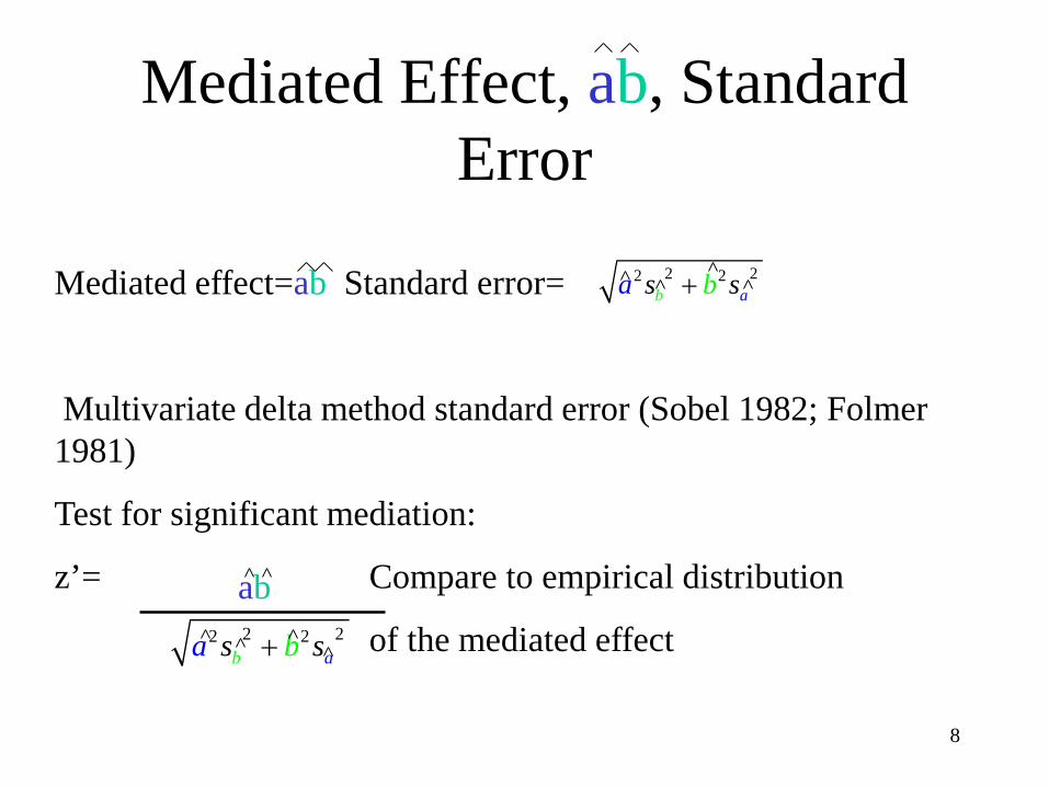
Mediated Effect, ab, Standard Error

8

Mediated effect=ab Standard error=

Multivariate delta method standard error (Sobel 1982; Folmer 1981)

Test for significant mediation:

z’= Compare to empirical distribution

of the mediated effect

2 22 2aba bs s+

ab2 22 2

aba bs s+

Reasons for Confidence Limits

Gives a range of values based on a sample estimate. Helps avoid binary, significant or not,

approach to research. Incorporates variability in the point estimate

as well as the point estimate.

9

Confidence Limits for ab

ba ˆˆ

bas ˆˆ

ba ˆˆ

ba ˆˆ

10

Confidence Limits ± zcrit

UCL = + zcrit

LCL = - zcrit

Where zcrit is the z critical value because the standard error is asymptotic. Valid to use t instead of z.

95% Confidence LimitsUCL = + 1.96 LCL = - 1.96

With normal distribution upper and lower critical values have the same value but opposite sign, e.g., 1.96 for z.975 and -1.96 for z.025

ba ˆˆbas ˆˆ

bas ˆˆ

bas ˆˆ

bas ˆˆba ˆˆ

11

Distribution of the Product The mediated effect is the product of two coefficients a

and b. The distribution of the product has a normal distribution only in special cases (MacKinnon et al., 2002). At low values of a and b, the distribution has excess

kurtosis and skewness, e.g. when a and b are both zero, kurtosis is 6. It is not surprising that the confidence limits are inaccurate if the distribution is assumed to be normal.One solution is to use the distribution of the product in

statistical tests and confidence limits.

Product of Two Normal Distributions is not always Normal

13

X ≠ ?

14

Plot of Kurtosis and Skewness of the Distribution of the Product

The next two plots show the kurtosis and skewness of the distribution of the product as a function of za= a/sa and zb=b/sb. The range of values for za and zb is from -4 to +4

in these plots. Applied research often has these zvalues, that is a z test for a and a z test for b range from -4 to 4. A normal distribution would have skewness and

kurtosis of 0 for all values of za and zb. The distribution of the product has different values of skewness and kurtosis for values of za and zb.

17

Critical Values for Distribution of the Product

Because the distribution of the product is not symmetric, there are different critical values for the distribution for each value of a/sa and b/sb. The critical values are -1.96 and +1.96 for the

95% confidence interval from the normal distribution. There are different upper and lower critical values for the distribution of the product. Confidence limits and significance tests are more accurate using the critical values from the distribution of the product (MacKinnon et al. 2004).

18

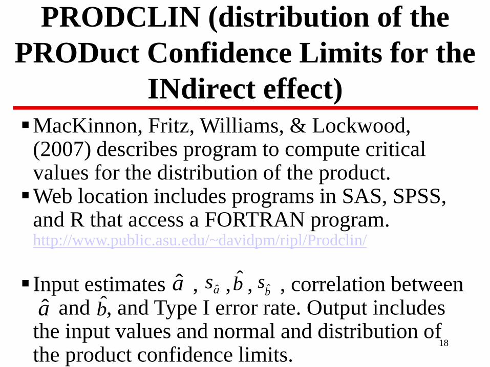
PRODCLIN (distribution of the PRODuct Confidence Limits for the

INdirect effect)MacKinnon, Fritz, Williams, & Lockwood,

(2007) describes program to compute critical values for the distribution of the product. Web location includes programs in SAS, SPSS,

and R that access a FORTRAN program. http://www.public.asu.edu/~davidpm/ripl/Prodclin/

Input estimates , , , , correlation between and , and Type I error rate. Output includes

the input values and normal and distribution of the product confidence limits.

a bba

as ˆ bs ˆ

http://www.public.asu.edu/%7Edavidpm/ripl/Prodclin/

19

RMediationTofighi & MacKinnon (2011) describes an R

program to find critical values for the distribution of the product that solves some problems in PRODCLIN, can get accurate results for cases where PRODCLIN did not converge, more accurate results for correlated z-values, makes plots of distributions and finds percentiles and probabilities.

Input estimates , , , , correlation between and , Type I error rate but input is now called

mu.x, se.x, mu.y, se.y, rho, alpha, respectively.

as ˆa b bs ˆ

a b

Assumptions I For each method of estimating the mediated effect

based on Equations 1 and 3 (c-c’) or Equations 2 and 3(ab): Predictor variables are uncorrelated with the error in

each equation. Errors are uncorrelated across equations (ab) . Predictor variables in one equation are uncorrelated

with the error in other equation. Reliable and valid measures No omitted influences. Normally distributed variables 20

Assumptions II Data are a random sample from the population of interest. Coefficients, a, b, c’ reflect true causal relations and the

correct functional form. Mediation chain is correct: Temporal ordering is correct

X before M before Y. Any mediation model is part of a longer mediation chain. The researcher decides what part of the micromediational chain to examine.

Homogeneous effects across subgroups: It assumed that the relation from X to M and from M to Y are homogeneous across subgroups or other characteristics of participants in the study. This means there are not moderator effects. 21

Identification Assumptions 1. No unmeasured X to Y confounders given covariates.2. No unmeasured M to Y confounders given covariates.3. No unmeasured X to M confounders given covariates.4. There is no effect of X that confounds the M to Y relation.

VanderWeele & VanSteelandt (2009) 22

Water Consumption Study Variables

Stimulus->Organism->Response study X is the temperature in degrees Fahrenheit M is a self-report of thirst at the end of the first

two hours of the study Y is the number of deciliters of water consumed

during the last two hours of the study 50 participants were in a room for four hours

doing a variety of tasks including sorting objects, tracking objects on a computer screen, and communicating via an intercom system

23

Water Consumption Study Purpose The purpose of the study was to investigate

whether persons can judge their water needs. Temperature should affect self-reported thirst which then should affect water consumption.

The accuracy of self-reported thirst is important because persons in self-contained environments need to monitor their own hydration.

The mediated effect of temperature on water consumption through self-reported thirst estimates the extent to which persons were capable of gauging their own need for water.

24

Water Consumption Study

25

SELF-REPORTED THIRST

M

TEMPERATURE

X Y

WATER CONSUMED

a

Temperature (X) to self-reported thirst (M) to water consumption (Y).

b

c’

SAS Program

proc reg;model y=x;model y=x m;model m=x;See handout for output.

26

SPSS Program

regression /variables x y m/dependent=y/enter=x.

regression/variables x y m/dependent=y/enter=x m.

regression/variables x y m/dependent=m/enter x.

See handout for output

27

Estimates of a, b, c, and c’(1) Temperature (X) was significantly related to

water consumption (Y) (c=.3604, sc=.1343, tc = 2.683).

(2) Temperature was significantly related to self-reported thirst (M) (a=.3386, sa=.1224, ta=2.767).

(3) Self-reported thirst was significantly related to water consumption controlling for temperature (b=.4510, sb=.1460, tb=3.090).

-The adjusted effect of temperature was not statistically significant, (c’=.2076, sc’=.1333, tc’=1.558) and there was a drop to c’ = .2076 from c=.3604. 28

Mediation Models for Water Consumption Data

Y = i1 + c X Y = -22.0505 + .3604 X

(.1343)

Y = i2 + c’ X + b M Y = -12.7129 + .2076 X + .4510 M

(.1333) (.1460)

M = i3 + a X M = -20.7024 + .3386 X

(.1224)

29


'ˆˆ cc −ba ˆˆ

30

Mediated effect

= (.3386) (.4510) = =.3604-.2076 =.1527

Standard error =

Standard error = 2 2 2 2.3386 (.1460) .4510 (.1224) .0741+ =

2ˆ

22ˆ

2 ˆˆ abFirst sbsas +=

31

Second Order Standard Error

2 2 2 2 2 2ˆˆ .3386 (.1460) .4510 (.1224) (.1224) (.1460) .0762Secondab

s = + + =

ˆˆ ˆ ˆ(.3386)(.4510) ' (.3604) (.2076) .1527ab c c= = − = − =

2ˆ

2ˆ

2ˆ

22ˆ

2 ˆˆ ababSecond sssbsas ++=

32

Confidence Intervals for the Mediated Effect First Order

Confidence intervals are advocated by researchers for several reasons: effect size, range of possible values, not just null hypothesis binary significance testing. For 95% confidence intervals:Upper Confidence Interval (UCL) = + z.975 s Lower Confidence Interval (LCL) = + z.025 s For water consumption data. UCL = .1527 + (1.96 )(.0741) = .2979 LCL = .1527 + (-1.96) (.0741) =.007595% Confidence Interval from .0075 to .2979. The

effect is statistically significant because 0 is not in the interval.

ba ˆˆ

ba ˆˆba ˆˆba ˆˆ

33

Confidence Intervals for the Mediated Effect Second Order

Confidence intervals are advocated by researchers for several reasons: effect size, range of possible values, not just null hypothesis binary significance testing. For 95% confidence intervals:Upper Confidence Interval (UCL) = + z.975 s Lower Confidence Interval (LCL) = + z.025 s For water consumption data.

UCL = .1527 + (1.96 )(.0762) = .3021 LCL = .1527 + (-1.96) (.0762) =.003395% Confidence Interval from .0033 to .3021. The

effect is statistically significant because 0 is not in the interval.

ba ˆˆ

ba ˆˆba ˆˆba ˆˆ

34

Example Calculations using the Distribution of the Product

For example, = .3386, = .1224, = .4510, = .1460. Enter these values in the PRODCLIN program. PRODCLIN uses the critical values for the 2.5%

percentile, Mlower =-1.6175 and Mupper = 2.2540 the critical value for the 97.5% percentile.Use the critical values to calculate upper and

lower confidence limits.LCL= + Mupper s = .1527 +(-1.6175) (.0741)

UCL= + Mlower s = .1527 + (2.2540 )(.0741)Asymmetric Confidence Limits are (.0329, .3197)

and (.0294, .3245) from new PRODCLIN.

ba ˆˆ

ba ˆˆba ˆˆ

ba ˆˆ

a as ˆ b bs ˆ

Plot and Confidence Limits from RMediation (Chapter 3 data)

35

36

More Examples

Was there a significant relation of X to M?

Was there a significant relation of M to Y adjusted for X?

Is the mediated effect statistically significant?

Word ExperimentPHLAME dataFit.txt data

1

Chapter 4: Simulations

Mediation equations. Other tests of mediation. Comparison of mediation tests. Statistical Simulation Studies

2

Mediation Regression Equations

Tests of mediation use information from some or all of the three equations. The coefficients in the equations may be

obtained using methods such as ordinary least squares regression, covariance structure analysis, or logistic regression.

3

Three Major Types of Single Sample Tests for the Mediation Effect

(1) Causal Steps (Baron & Kenny, 1986; Judd & Kenny, 1981). (2) Difference in Coefficients: estimator (e.g.,

Clogg et al., 1992) (3) Product of Coefficients: estimator (e.g.,

Sobel, 1982) See MacKinnon et al. (2002), Psychological

Methods article for a review and comparison of single sample tests

ba ˆˆ

'ˆˆ cc −

4

Causal Steps Tests of Mediation Causal Step 4 from Judd & Kenny (1981):

test that = 0 is nonsignificant (i.e., complete mediation required). Causal Step 4 from Baron & Kenny (1986):

drop in magnitude of sample estimates from to Test of joint significance: test whether the

and paths are statistically significant (MacKinnon et al., 2002).

'c

'cc

ba

5

Equation 1

MEDIATOR

M


X Y

DEPENDENT VARIABLE

c


6

Equation 2

MEDIATOR

M


X Y

DEPENDENT VARIABLE

2. The independent variable is related to the potential mediator:

a

7

Equation 3

MEDIATOR

M


X Y

DEPENDENT VARIABLE

a

3. The mediator is related to the dependent variable controlling for exposure to the independent variable:

b

c’

8


Indirect Effect = Mediated effect = ab = c-c’

Direct effect= c’

Total effect= ab+c’=c

9

Product of Coefficients

2ˆ

2ˆ

2ˆ

22ˆ

2 ˆˆbaabSecond sssbsas ++=

2ˆ

2ˆ

2ˆ

22ˆ

2 ˆˆbaabUnbiased sssbsas −+=

2ˆ

22ˆ

2 ˆˆ abFirst sbsas +=

Corresponding standard errors of ab:

10

Difference in Coefficients

General standard error formula:

Clogg, Petkova, and Shihadeh (1992) variance:

Covariance between c and c’, McGuigan & Langholz (1988) generalized to more cases by MacKinnon et al. (2002)

2 2ˆ ˆ ˆ ˆ ˆ ˆ ˆ ˆ' ' ' '2c c c c cc c cs s s r s s− = + −

2ˆ ˆ ˆ' 'c c c XMs s r− =

2ˆ ˆ ˆ ˆ ˆ ˆ' ' ' / (( )( ))cc cc c c Xs r s s MSE s N= =

11

Tests evaluated

(1) Baron & Kenny Causal Steps (Baron & Kenny, 1986)(2) Joint Significance test (MacKinnon et al., 2002)(3) Delta Method is the first order standard error of ab

(Sobel, 1982).(4) Distribution of the Product (MacKinnon et al., 2002)

uses the distribution of the product to form a confidence intervals and assesses significance by evaluating whether 0 is in the confidence interval.

(5) Lots of other tests evaluated in the simulation study. Resampling tests will be described later, e.g., the bootstrap. See the cited articles for more on these tests.

12

Steps in a Statistical Simulation

(1) Generate sample data under a known population model.(2) Estimate model coefficients and standard errors in the

sample. (3) Save the estimates, standard errors, and results of

statistical tests in the sample.(4) Repeat Steps 1 to 3 a large number of times. The number

of times that steps 1-3 are repeated are the replications.(5) Compare results across all replications to the population

values. Which tests led to the most accurate decisions about the population value?

13

Simulation Design: MacKinnon et al., 2002

All possible combinations of a, b, and c’ effect sizes for zero, small (2% variance explained), medium (13%), and large (26%) effects.5 Sample sizes, N= 50, 100, 200, 500, and 1000500 Replications of each of the 4 X 4 X 4 X 5

generated data sets.Type I error and Power 14 TestsCausal step, difference in coefficients, and

product of coefficients tests.

14

Simulation Results: MacKinnon et al., (2002) Conclusions

Taking all situations, both paths zero, one path zero and the other path nonzero for Type I error rates, and power for nonzero mediation relations.

Tests differ widely in statistical performance.

Best tests are: (1) the joint significance test of the a and b paths

(2) a test based on formingconfidence limits using the distribution of the product (test significance by whether 0 is in the confidence interval).

15

Reasons for Differences Among Methods

Requirement for significant total effect, c, and requirement that c’ is nonsignificant reduces statistical power of BK and JK causal steps methods.

Assumption that the mediated effect divided by its standard error has a normal distribution is incorrect in some situations.

Mediation is fundamentally a test of two paths corresponding to the a and b paths.

16

Fritz & MacKinnon, 2007

Purpose of the study is to obtain required sample size to have .8 power to detect the mediated effect given population values of a, b, and c’ effect sizes for small (S), medium (M), halfway between small and medium (H), and large (L) effects.Table 3 presents these values for Baron & Kenny,

joint significance, Delta (first order), PRODCLIN, percentile bootstrap, and bias-corrected bootstrap methods. Required sample size determined empirically

using a iterative procedure.

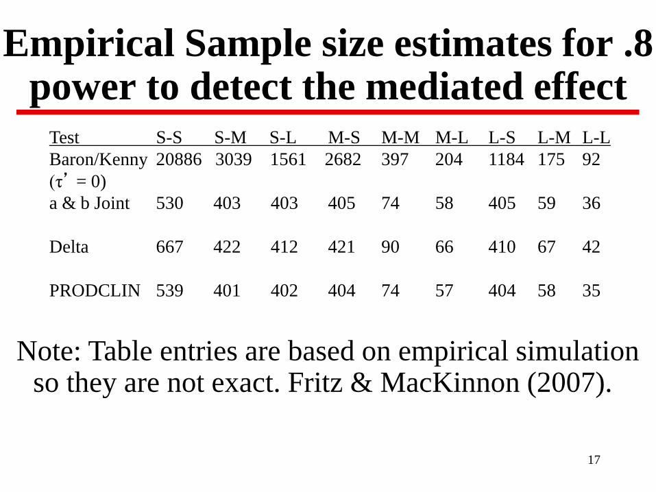
17

Empirical Sample size estimates for .8 power to detect the mediated effect

Test S-S S-M S-L M-S M-M M-L L-S L-M L-LBaron/Kenny 20886 3039 1561 2682 397 204 1184 175 92(τ’ = 0)a & b Joint 530 403 403 405 74 58 405 59 36

Delta 667 422 412 421 90 66 410 67 42

PRODCLIN 539 401 402 404 74 57 404 58 35

Note: Table entries are based on empirical simulation so they are not exact. Fritz & MacKinnon (2007).

18

Results: Fritz & MacKinnon, 2007 Sample size requirements are large for .8 power to detect a

mediated effect—around 400 if one of the effects is not small. Excessive sample size requirements for the Baron & Kenny

method because of the requirement for a significant total effect c. This occurs because when the direct effect is zerothe value of c is the product of the two paths in the mediated effect. So if both paths are small then the total effect is the product of two small effects. Excessive sample size for .8 power to detect c for the

product of two small mediation paths is correct (p. 238). Best tests: joint significance, distribution of the product or

bias-corrected bootstrap (there is some evidence that the bias-corrected bootstrap has increased Type I error rates in some, albeit rare, situations).

19

New Methods for Power for Complex Mediation Models

Thoemmes, MacKinnon, & Reiser (2010) describe a general procedure to calculate power for any mediation model. The paper uses Mplus to conduct the power calculations. Some of the models covered in that paper are multiple

mediator models, latent variable models, moderator and mediator models, and longitudinal mediation models. This does require that you can come up with educated

guesses of the parameter values and variability for many different parameters.

Thoemmes, F., MacKinnon, D. P., & Reiser, M. R. (2010). Power Analysis for Complex Mediational Designs Using Monte Carlo Methods. Structural Equation Modeling, 17, 510-534.

20

Mediation as a Way of Increasing Power

O’Rourke and MacKinnon (2013) discuss situations in which including a mediator will increase power to detect effects over a bivariate relation between X and YWhen ab is equal to c (c’ is zero), the test of mediation will

always have more power than the test of the total effect This occurs when the standard error of c is larger than the

standard error of ab. These results also apply to the two mediator and sequential

mediation models.

O’Rourke, H. P., & MacKinnon, D.P. (2015). When the test of mediation has more power that the test of the total effect. Behavior Research Methods, 47, 424-442.

Ways to increase statistical power: Fritz, M. S., *Cox, M. G., & MacKinnon, D. P. (2015). Increasing Statistical Power in Mediation Models without Increasing Sample Size. Evaluation and the Health Professions, 38(3), 343-366.

21

Confidence Limits (MacKinnon, Lockwood, & Williams, 2004)

Many single sample tests have low powerEarlier studies (MacKinnon et al., 1995) found

that confidence limits for the mediated effect are imbalanced especially for small sample sizes and small effect sizesSome problems with testing for mediation

because the distribution of the product is normal only in special cases. Resampling methods may solve the problem.

22

Options to make Confidence Limits

Normal theory yields symmetric confidence limits.

Distribution of the Product for asymmetric confidence limits.

Resampling methods for asymmetric confidence limits—many different types of resampling methods including the bootstrap and jackknife.

Which confidence limits are the most accurate?

23

Resampling Steps: Confidence Limits

1. Estimate mediated effect in the original sample2. Generate new data based on rearranging or

sampling original data3. Calculate effect in the generated data4. Repeat steps 2 and 3 a large number of times5. Create empirical distribution of the effect from

generated and original data6. Compute UCL and LCL in the empirical

distribution

24

Resampling Simulation Design10 combinations of effect size for the a and b paths:

z,z; z,s; z,m; z,l; s,s; s,m; s,l; m,m; m,l; l,l 4 Sample sizes, N= 25, 50, 100, and 2001000 Replications so there are 4 X 10 X 1000 =

40,000 generated data sets in Study 1. But there are also 1000 resamples in Study 2 so that there are actually, 40,000,000 data sets in that study.Study 1 compared normal and distribution of the

product confidence limits. Study 2 evaluated many resampling testsType I error, Power, Confidence limit coverage

25

Results (MacKinnon, Lockwood, & Williams, 2004) #1

Study 1 demonstrated the superiority of the distribution of the product confidence limits over the normal theory confidence limits.Study 2 demonstrated that resampling methods

work as well as the distribution of the product and both are better than normal theory based confidence limits

26

Results (MacKinnon, Lockwood, & Williams, 2004) #2

Bias-corrected bootstrap most accurate overall but can be cumbersome and there are situations where the Type I error rate is over .05 (see Fritz et al., 2012). Percentile method works well.

Bootstrap is available in Amos (Arbuckle & Wothke, 1999) EQS (Bentler, 1997), LISREL (Joreskog & Sorbom, 2001), Mplus (Muthen & Muthen) and a SAS program (Lockwood & MacKinnon, 1998), SAS and SPSS (Preacher & Hayes, 2008)

Single sample Distribution of the Product CL is the best single sample method and does not have cases where the Type I error rate is as high as the bias-corrected bootstrap.

27

Other Mediation Simulation StudiesInconsistent Mediation (MacKinnon, Krull, & Lockwood,

2000, Prevention Science).Logistic and probit regression (MacKinnon et al. 2007,

Clinical Trials). Path Analysis models (Williams & MacKinnon, Structural

Equation Modeling, 2008)Multilevel models. (Krull & MacKinnon, 2001)Pituch, Whittaker, & Stapleton (2005) replicated superior

results of the distribution of the product methods (Multivariate Behavioral Research)

Bayesian Mediation Analysis (Yuan & MacKinnon, 2009, Psychological Methods.

Median Regression Mediation Analysis (Yuan & MacKinnon 2014, Psychological Methods)..

28

Gary Larson

1

Computer Intensive Methods (Chapter 12)

Purpose is to use the data itself to form a distribution of a statistic (Manly, 1997). Does not make as many assumptions and can handle nonnormal distributions.

The value of a statistic in the observed sample is compared to the distribution of the statistic formed by resampling from the observed data a large number of times.

Bootstrap method for mediated effects described by Bollen & Stine (1991), Lockwood & MacKinnon (1998), and Shrout & Bolger (2002)

2

Options to make Confidence Limits

Normal theory yields symmetric confidence limits.

Distribution of the Product for asymmetric confidence limits.

Resampling methods for asymmetric confidence limits—many different types of resampling methods including the bootstrap and jackknife.

3

Bootstrap Confidence Limits

1. Estimate mediated effect in the original sample2. Generate new data based on sampling with

replacement from the original data3. Calculate effect in the generated data4. Repeat steps 2 and 3 a large number of times5. Create empirical distribution of the effect from

generated and original data6. Compute UCL and LCL in the empirical

distribution.

4

Bootstrap in groups Observed Data set with N = 6

Obs X M Y1 1 2 -42 1 5 -63 2 8 -144 2 9 -165 -1 -7 126 0 0 -1

5

Bootstrap Sample 1Six rolls of the dice gave, 1, 5, 2, 3, 1, 2

Obs x m y1 1 2 -45 -1 -7 122 1 5 -63 2 8 -141 1 2 -42 1 5 -6

So this is a bootstrap sample. Note that sampling is with replacement so observations 1 and 2 are repeated twice and observations 4 and 6 were not sampled. The mediated effect would be calculated for this sample and the process is repeated a large number of times.

6

Group MembersRandomizer rolls the die.

Recorder writes the data.

Analyzer analyzes the data.

Reporter describes results.

7

Bootstrap samplingRandomizer rolls the die 6 times and records the

number for each roll. These are the Obs numbers of participants selected for the bootstrap sample.

Recorder writes the data for X, M, and Y for each Obs number. Note that Obs numbers could be in the sample several times.

Analyzer types the bootstrapped data in SAS and estimates the mediated effect. You will be asked for your the mediated effect in your sample.

Reporter reports the value of the mediated effect for the bootstrap sample.

8

Bootstrap Confidence Intervals Write down the mediated effect from each bootstrap sample. Form a distribution of the bootstrap sample estimates of the

mediated effect. Order mediated effects from large to small for bootstrap and original sample: -15.7234, -6.4202, -5.1223, -.3.2241, -1.9433, 0.34… (a sample could be undefined because could not be estimated)

Find the value of the mediated effect in the bootstrap samples corresponding to the 2.5% and 97.5%. These are the bootstrap 95% confidence intervals.

Confidence limits require a large number of bootstrap samples, such as 1000 so that the confidence limits are the 2.5th and 97.5th values in the bootstrap distribution.

Best to use a computer program to do the bootstrap sampling and analysis. It would take us a while to take 999 bootstrap samples.

b

LCL=-12.672.5%

UCL=3.5697.5%

95% Confidence Interval

10

Bootstrap Confidence Intervals

95% Confidence interval from Percentile bootstrapLCL = -12.667 and UCL =3.556

95% Confidence interval from Bias-Corrected BootstrapLCL = -13.2 UCL = 2.706

Percentile Bootstrap mean = -6.3578Percentile Bootstrap Median = -5.8728Bias-corrected bootstrap makes a new percentile for the LCL and UCL based on the discrepancy between the observed mediated effect and average bootstrap mediated effect.

11

Mplus Mediation Analysis Mplus will estimate mediated effects and their standard

errors. MODEL INDIRECT: Y IND X; estimates indirect

effects from X to Y and standard errors. For the single mediator model there is one indirect

effect from X to M to Y and one standard error. For multiple mediator models there may be many

mediated effects from X to Y. Each of the individual mediated effects are called specific mediated effects and Mplus will estimate each specific mediated effect and compute a standard error for each specific mediated effect.

The data here have one mediator so there is one mediated effect.

12

Mplus Bootstrap Analysis Mplus will estimate mediated effects and conduct

bootstrap sampling Analysis: Bootstrap=1000: specifies 1000 bootstrap

samples OUTPUT: Cinterval; to obtain normal distribution

confidence intervals. OUTPUT: Cinterval(bootstrap) to obtain bootstrap

confidence intervals. OUTPUT: Cinterval(bcbootstrap) to obtain bias-

corrected bootstrap confidence intervals. Bias corrected bootstrap confidence intervals adjust the interval to reflect that the average bootstrap mediated effect is not the same value of the mediated effect in the original sample (see Chapter 12).

See Mplus Handout

13

How the data were generated. The data were generated with population values of a =

4 (true standard error of .25), b = -2 (.333), and c’ = 1(.333) so the population mediated effect, ab, was -8 and the true standard error of the estimated mediated effect was equal to 2.5331 so the true z’ equals 3.1582.

In summary, six observations were generated from a population with a real mediated effect of -8. So the correct decision is to say that there is a mediated effect in these data. Normal theory analysis of these data and the bias corrected bootstrap led to the correct conclusion but the percentile bootstrap did not.

14

Bootstrap ‘mediation’

mediation

deiamanniedadedetnoedeatdoodamoatnmmnmadnatid

15

Resampling Methods Summary Now widely used method for a variety of reasons,

applicability in complicated situations where analytical solutions are not known or untenable.

Useful for mediation analysis because it can be used for any mediation model with complex mediated effects when the distribution of the effects is not known.

Some limitations: generalizing beyond the sample at hand may not be appropriate, software can be difficult to implement, and Gleser’s law, “Two individuals using the same statistical method should arrive at the same conclusion.”

Other Resampling Methods: Permutation, bootstrap t, bootstrap Q, Jackknife, Monte Carlo…

1

Measures of Effect Size (Chapter 4)

There are several measures of effect size for the mediation model

Effect size measures for individual paths Effect size measures for the mediated effect

2

Measures of Effect Size for Paths

Correlation between X and M for the coefficient.

Partial correlations for and . Correlation of .1, .3, and .5 correspond to small, medium, and large effects (Cohen 1988)

Standardized betas for , , and . Change in standard deviations in the dependent variable for a standard deviation change in the independent variable

a

b 'c

b 'c a

3

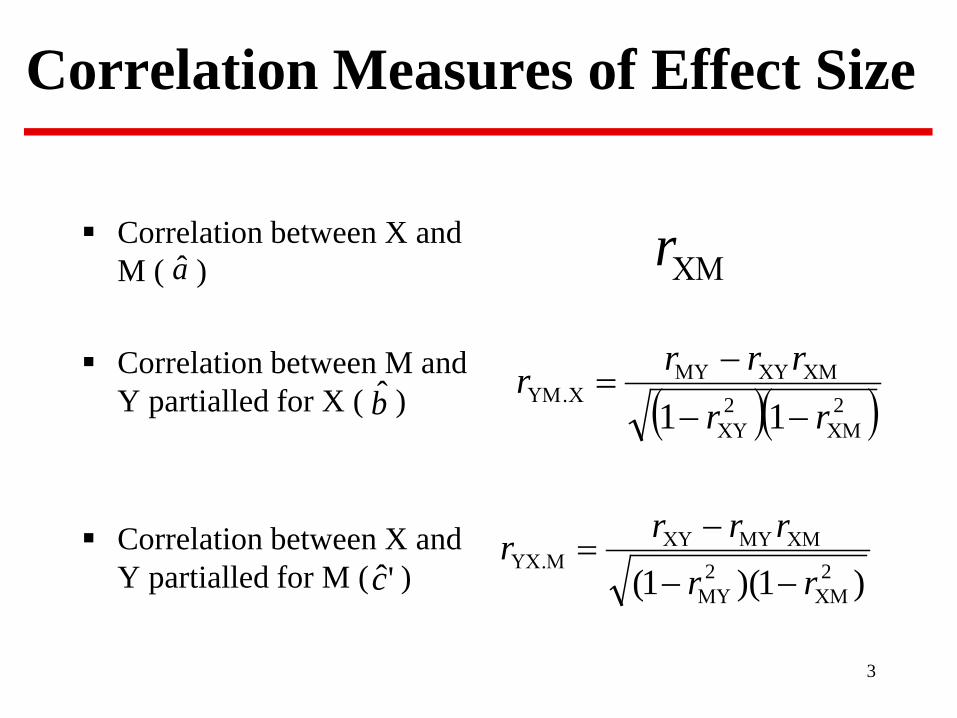
Correlation Measures of Effect Size

Correlation between X and M ( )

Correlation between M and Y partialled for X ( )

Correlation between X and Y partialled for M ( )

ΧΜr

)1)(1( 22.

ΧΜΜΥ

ΧΜΜΥΧΥΜΥΧ

−−

−=

rrrrrr

( )( )22.11 ΧΜΧΥ

ΧΜΧΥΜΥΧΥΜ

−−

−=

rrrrrr

a

b

'c

4

Standardized Beta Measures of Effect Size

Standardized Beta between X and M ( )

Standardized Beta between M and Y adjusted for X ( )

Standardized Beta between X and Y adjusted for M ( )

2ˆ

1Sr r rb

rΜΥ ΧΜ ΥΧ

ΧΜ

−=

−

2ˆ '1S

r r rcr

ΧΥ ΧΜ ΥΜ

ΧΜ

−=

−

Ms rΧ=aa

b

'c

5

Effect size for the water consumption study

Correlation and partial correlation effect size measures were: = .371

= .411= .222 = .361

Standardized betas were: = .371 = .413= .208 = .361

ab

c

c

ab

'c

'c

6

Effect size for Word Experiment Data

Correlation and partial correlation effect size measures were: = .623

= .390= .040 = .337

Standardized betas were: = .623 = .470= .044 = .337

b

b

a

a

c

c

'c

'c

7

Measures of Mediated Effect Size

Proportion mediated:

(Estimators are equal for OLS regression but not for logistic and probit regression)

Ratio of mediated to direct effect:

R-squared attributable to the mediated effect:

−=

+=

cc

cbaba

cba

ˆ'ˆ1

'ˆˆˆ

ˆˆˆ

ˆˆ

'ˆ

ˆˆcba

)( 22,

2YXMXYYM rRr −−

8

Mediated effect size in the Water Consumption study

Proportion mediated was =.1527/.3604 = .4238

42% of the total effect of X on Y was through the mediator M.

Ratio of indirect to direct effect was = .1527/.2076=.7354 The mediated effect was .74 the size of the direct effect

controlling for the mediator.

R2 attributable to the mediated effect was R2med = (.2399-(.2772-

.1304)) = .0931

cbaˆ

ˆˆ

'ˆ

ˆˆcba

9

Mediated effect size in the Word Experiment Data

Proportion mediated was =2.185/2.517 =.868

Ratio of indirect to direct effect was = 2.185/.332=6.58

R2 attributable to the mediated effect was R2med =

(.2476-(.2488-.1137)) = .1125

cbaˆ

ˆˆ

'ˆ

ˆˆcba

10

Other Effect Size Measures:Water Consumption Example

Mediated effect in terms of standard deviations of the dependent variable, Y (MacKinnon, 2008).

Water consumption value was .1343 = (.1527/1.134) For a one-unit increase in X, Y increases by .13 standard

deviations due to mediation.

Surrogate endpoint and correlation between M and Y. The ideal surrogate = 1 and rMY equals 1.

Water consumption data = .613= (.2076/.3386) and rMY equals .489

acˆˆ

acˆˆ

acˆˆ

𝑆𝑆𝑆𝑆𝑆𝑆𝑆𝑆𝑆𝑆𝑆𝑆𝑆𝑆𝑆𝑆𝑆𝑆𝑆𝑆𝑆𝑆𝑆𝑆𝑆𝑆�𝑏𝑏� = 𝑆𝑆�𝑏𝑏�𝑠𝑠𝑦𝑦

11

Other Effect Size Measures:Word Experiment Data

Mediated effect in terms of standard deviations of the dependent variable, Y (MacKinnon, 2008).

Word class experiment value was .5812=(2.185/3.7594)

Surrogate endpoint and correlation between M and Y. The ideal surrogate = 1 and rMY equals 1.

Water consumption data = .7073= (2.5167/3.5583) and rMY equals .4976

acˆˆ

acˆˆ

acˆˆ

𝑆𝑆𝑆𝑆𝑆𝑆𝑆𝑆𝑆𝑆𝑆𝑆𝑆𝑆𝑆𝑆𝑆𝑆𝑆𝑆𝑆𝑆𝑆𝑆𝑆𝑆�𝑏𝑏� = 𝑆𝑆�𝑏𝑏�𝑠𝑠𝑦𝑦

12

Additional Effect Size Measures

Mediated effect standardized by standard deviation of both X and Y (Alwin & Hauser, 1975; Cheung, 2009).

k2 (Preacher & Kelly, 2011, Psychological Methods) Proportion of the maximum possible indirect effect. Divide the observed mediated effect by the largest possible value of ab that could be obtained given the data. The largest possible mediated effect is a function of the observed variances and covariances among X, M, and Y. Problems with k2 owing to nonmonotonicity shown by Wen & Fang, (2015: Psychological Methods).

ˆˆ X

Y

sabs

13

Additional Effect Size Measures Water Consumption Data

ab standardized by standard deviation of X and Y

Water Consumption Data =

For a one standard deviation increase in X, Y increases by .15 standard deviations due to the mediated effect.

k2 for Water Consumption Data = .153/.992=.154

The observed proportion of the maximum possible indirect effect is .15.

ˆˆ X

Y

sabs

1.137ˆˆ .1527 .1531.135

X

Y

sabs

= =

14

Additional Effect Size Measures Word Experiment Data

Mediated effect standardized by standard deviation of X and Y

Word Spring 2012 Data =

k2 for Word Data =2.185/8.843=.2471

Proportion of the maximum possible indirect effect.

.5037ˆˆ 2.185 .29283.7594

X

Y

sabs

= =

15

Standardized Effect Size Measures

Mediated effect in terms of the change in standard deviation units of Y for a one unit change in X. Useful for binary X or when one unit change is desired. (Mplus STDY)

Mediated effect in terms of the change in standard deviation units of Y for a one standard deviation change in X. Useful for continuous X. (Mplus STDXY)

ˆˆ X

Y

sabs

ˆˆ

Y

abs

16

Simulation Results Mackinnon, Warsi, & Dwyer (1995), Marcia Taborga’s

masters thesis, MacKinnon, Fairchild, Yoon, & Ryu (2007), and Fairchild, MacKinnon,Taborga, & Taylor (2009 ).

Correlation and standardized beta values for individual paths work well at reasonable sample sizes of 50 etc.

Ratio requires at least N of 1000. Proportion requires sample size of 500 unless effect sizes are large then OK for as small as 100. Standardized mediated effect and mediation R-squared seem to work reasonably well and show promise at small sample sizes.

More work needs to be done but at this point standardized effect sizes are recommended.

17

Simulation Results (continued) Some work evaluating the bias and stability from

sample to sample of ab/sY, ab(sX)/sY, k2, the proportion, and ratio mediated showed that ab/sY, ab(sX)/sY, and k2 have lower relative bias and more stability than the proportion and ratio mediated even at sample sizes as low as N=10 (Miočević, O’Rourke, & MacKinnon, 2014).

You can report more than one effect size for a given study; some effect sizes have more intuitive interpretations for your data.

18

SummaryEffect sizes for individual paths in the mediated effect and

also the mediated effect.

Use correlation and standardized betas for individual paths.

Standardized mediated effect measures are reasonable either for a one unit change in X or a standard deviation change in X. The proportion mediated is widely used but may not be stable at smaller sample sizes.

Can derive standard errors for any function using the multivariate delta method. Could also use the bootstrap to find confidence intervals and Bayesian estimation to find the credibility intervals. Can do this with the Mplus MODEL CONSTRAINT command.

19

When a third variable increases or reverses the relation between X and Y. In most situations, the relation between X and Y is reduced when

the third-variable is included because it is a mediator or a confounder and it explains part of the relation of X and Y. There are cases where the X to Y relation gets bigger or reverses sign when a third variable is included.

A suppressor variable is a variable that increases the magnitude of the relation between X and Y when it is included in the analysis.

A distorter variable changes an X to Y relation such that when it is included, a relation emerges or changes in sign.

A suppressor or distorter could be a mediator or confounder. A covariate is not a suppressor or distorter because it does not

change the relation between X and Y.

20

Suppressor Example

Horst (1941) evaluated the relation between mechanical ability and pilot performance. The relation increased when verbal ability was included.

Mechanical ability and pilot performance are strongly related. It takes verbal ability to complete the mechanical ability test. So removing verbal ability from the test, yields a more accurate (and larger) estimate of mechanical ability and pilot performance.

So magnitude of the relation between mechanical ability and pilot performance increased when verbal ability was included. It is a confounder not a mediator because it doesn’t really make sense that mechanical ability causes verbal ability which causes pilot performance.

21

Distorter Example 1

A distorter third-variable reverses the sign of the relation between X and Y or changes a zero relation between X and Y to a nonzero relation.

Positive relation between suicide rate and marital status overall. More likely to commit suicide if married seems unusual. When age is included in these analyses, there is a negative relation between marriage and suicide rate for each age (Rosenberg, 1968, p. 84). Age is a confounder not a mediator because age does not make sense as a mediator between marriage and suicide.

22

Distorter Example 2A distorter variable exhibits what has been called the

Simpson’s paradox, also known as the reversal paradox (also Lord’s paradox). These effects occur when the overall relation between two variables differs from the relation across levels of the confounding variable.

Two Treatments for kidney stones: Treatment A was best both for small 93% vs 87% success and large 73% vs 69% kidney stones but Treatment B was better if size of stone was not considered 78% versus 83% success. The overall relation of treatment to success differs from the adjusted effect because of different sample sizes in each group.

23

Distorter

“one may be equally misled in assuming that an absence of relation between two variables is real, whereas it may be due .. to the intrusion of a third variable” (Rosenberg, 1968, p. 84).

24

Inconsistent Mediation Models

Inconsistent mediation models occur when the relation of X to Y increases in magnitude when the mediator is included in the analysis (see MacKinnon, Krull, & Lockwood 2000).

There is a mediation relation because the mediator transmits the effect of the independent variable to the dependent variable. Inconsistent mediation can occur whether or not c is statistically significant. The only requirement is that c’ is larger in magnitude than c.

Are inconsistent mediation effects rare?

25

Inconsistent MediationExample: Delinquency

Program to reduce juvenile delinquency brings high risk persons together for a special program. But the program increases the social norm that juvenile delinquency is common and that social norm increases subsequent delinquency. But overall, the program reduces juvenile delinquency.

X

DelinquencyNorm

Rearrest

+

-

+

26

Inconsistent MediationExample: Incarceration

Incarceration increases rehabilitation and rehabilitation reduces rearrest. But overall, incarceration increases rearrest because of exposure to pro-crime norm, for example.

X

Rehab.

Rearrest+

-+

27

Inconsistent MediationExample: Drug Prevention

Drug prevention increases curiosity about drugs. But overall, prevention reduces drug use behavior. (Matt)

X

Curiosity

Drug Use

++

-

28

Inconsistent MediationExample: STD Prevention

Condom promotion increases interest in sex which increases interest in sex (A criticism of safe sex interventions). But overall condom promotion reduces unsafe sex. (Amanda G.)

X

Interest

Unsafe Sex

++

-

29

Inconsistent MediationExample: Obesity Prevention

Obesity prevention increases interest in food which increases overeating. But overall the program reduces overeating. (Angela)

X

Interest

Behavior

++

-

30

Inconsistent MediationExample: Steroid Prevention

Steroid prevention program increases reasons to use steroids and reasons to use steroids increases intentions to use steroids. But overall the intervention reduces intentions to use steroids (MacKinnon et al., 2000).

X

Reasons

Intent

++

-

31

Inconsistent mediation in ATLAS Data

REASONS TO USE AAS

M

PROGRAM

X Y

INTENTION TO USE AAS

.573 (.105) .073 (.014)

-.181 (.056)

Mediated effect = .042 ( =.011) Direct effect = -.181 ( =.056);Total effect = = -.139 =.056

bas ˆˆba ˆˆ'c 'cs c cs ˆ

32

Mediators of age on typing (Salthouse, 1984)

Reaction

TimeM1

X Y

Age Typing

Proficiency

+

+

-

33

Multiple Mediator Model Preview: Opposing mediators for the null effect of age on typing

(Salthouse, 1984; Baltes & Baltes,1990)

Reaction

TimeM1

X YSkill

M2

+

Age Typing

Proficiency

+

+

0

-

34

Inconsistent Mediation Models Summary


Are there types of inconsistent mediation relations?Interest, norm, opposing mediation effects…

More on inconsistent mediation in multiple mediator models. An inconsistent mediation model has at least one mediated effect that has a different sign than the direct effect or other mediated effects.

1

Single Mediator Model So Far

Three Regression EquationsEstimates of the mediated effect, significance testing and confidence limitsSimulation study results for significance testing and confidence limit estimationReasons for discrepancies among testsMediator and Confounder RevisitedInconsistent Mediation RevisitedEffect Size

2

Three Major Types of Single Sample Tests for the Mediation Effect

(1) Causal Steps: Series of tests described in Baron & Kenny (1986) and Judd & Kenny, (1981).(2) Difference in Coefficients: estimator, e.g., from Clogg et al. (1992)(3) Product of Coefficients: estimator, e.g., from Sobel (1982)

ba ˆˆ

'ˆˆ cc −

3

Three Mediation Equations

Y= i1+ c X + e1

Y= i2+ c’ X + b M + c2

Y= i3+ a X + e3

With XM interactionY= i4+ c’ X + b M + h XM + e4

4

Significance Testing and Confidence Limits

Recommend product of coefficients estimation of the mediated effect and standard error. Recommend joint significance, distribution of the product, and bootstrap for confidence limit estimation and significance testing. Bias-corrected bootstrap has the most power but can have slightly higher Type I error rates that occur in rare circumstances.

Note that now the distribution of the product test is only available for two-path mediated effects. Joint significance and resampling methods work for any model even complicated ones.

5

Reasons for Differences Among Methods

Requirement for significant total effect, c, and requirement that c’ is nonsignificant reduces statistical power of BK and JK causal steps methods.Assumption that the mediated effect divided by its standard error has a normal distribution is incorrect.Mediation is fundamentally a test of two paths corresponding to a and b paths.

6

What is the problem with requiring c to be statistically significant? #1

Can drastically reduce power to detect a mediation effect and power is reduced as mediation approaches complete mediation. Ironic that use of this criteria leads to lowest power for complete mediation models when complete mediation is the most defensible mediation conclusion from a research study.

Subgroups of persons who have opposing mediated effects, e.g. mediation relation for males is opposite of that for females so c is nonsignificant when sex is ignored.

Test of c, is a statistical test that can be wrong (Type 1 and 2 Errors). Because the null hypothesis of c = 0 is not rejected does not mean that it should be accepted that c = 0 (same as any null hypothesis).

7

What is the problem with requiring c to be statistically significant? #2

Test of ab is more powerful than test of c, i.e., mediation more precisely explains how X affects Y.

Lack of statistically significant c is very important for mediation analysis because failure of action, conceptual, or both theories is critical for future studies.

Inconsistent mediation relations are possible because adding a mediator may reveal a mediation relation.

Note the test of c is important in its own right but is a different test than the test for mediation.

8

When the test of Mediation has more power that the test of the Total Effect?

The test of ab has more power than the test of c when effects are small and sample size is large, and when effects are large and sample size is small.

When ab is equal to c, the test of ab is always more powerful than the test of c.

This occurs because the standard error of c is larger than the standard error of ab.

O’Rourke, H. P., & MacKinnon, D.P. (2015). When the test of mediation has more power that the test of the total effect. Behavior Research Methods, 47, 424-442.

9

Breaking Down the Mediated Effect: Conceptual Theory Failure

• Conceptual theory outlines how hypothesized mediators are linked to outcomes of interest. – Are these the right mediators? Are they causally related to the

dependent variable?

Y

a

c’

b

ConceptualTheory

X

M

10

Breaking Down the Mediated Effect: Action Theory Failure

• Action theory outlines how a manipulation, X, relates to hypothesized mediators– Can these mediators be changed? How do we change these

mediators?

Y

α

c’

b

ActionTheory

X

M

11

Mediator, Confounder, Moderator, Covariate

• Mediator-a variable that is intermediate in a causal sequence such that X causes the mediator and the mediator causes Y. The relation between X and Y changes when adjusted for the mediator.

• Confounder-a variable that is related to both X and Y but is not in a causal mediation sequence. The relation between X and Y changes when adjusted for the confounder.

• Covariate- a variable that is related to X or Y or both. The relation between X and Y does not appreciably change when adjusted for the covariate.

• Moderator-a variable where the relation of X to Y is different at different values of the moderator.

12

When a third variable increases the relation between X and Y.

In most situations, the relation between X and Y is reduced when the third-variable is included because it is a mediator or a confounder and it explains part of the relation of X and Y. There are cases where the X to Y relation gets bigger or reverses sign when a third variable is included.A suppressor variable is a variable that increases the magnitude of the relation between X and Y when it is included in the analysis.A distorter variable changes an X to Y relation such that when it is included, a relation emerges or changes in sign. A suppressor or distorter could be a mediator or confounder.A covariate is not a suppressor or distorter because it does not change the relation between X and Y.

13


Inconsistent mediation models occur when the relation of X to Y increases in magnitude when the mediator is included in the analysis (see MacKinnon, Krull, & Lockwood 2000).

There is a mediation because the mediator transmits the effect of the independent variable to the dependent variable. Inconsistent mediation can occur whether or not c is statistically significant. The only requirement is that c’ is larger in magnitude than c.

14


REASONS TO USE AAS

M

PROGRAM

X Y


.573 (.105) .073 (.014)

-.181 (.056)

Mediated effect = .042 ( =.011) Direct effect = -.181 ( =.056);Total effect = = -.139 =.056

bas ˆˆba ˆˆ'c 'cs c cs ˆ

15



More on inconsistent mediation in multiple mediator models. An inconsistent mediation model has at least one mediated effect that has a different sign than the direct effect or other mediated effects.

16

Effect SizeEffect sizes for individual paths in the mediated effect:

correlation and standardized regression coefficients.

Effect sizes for the mediated effect: standardized mediated effect, proportion mediated, R2 mediated, proportion of total possible mediated effect.

Can obtain confidence intervals and tests of significance by deriving the standard error of any function of random variables with the multivariate delta method. Can also use the bootstrap to obtain confidence intervals.

17

SummaryEven the single mediator model is complex. Regression coefficients are used to obtain estimates of the

different effects in the mediation model.Significance testing and confidence limit estimation

complicated by the non-normal distribution of the product. Consistent and Inconsistent mediation models.Product of coefficient methods extend to more complicated

models.Some methods and statistics will no longer be appropriate for

more complicated models.More complicated mediation models primarily address

violations of assumptions of the single mediator model, such as omitted variable bias, temporal precedence, measurement error, moderation and mediation, categorical data, multilevel data….

Multiple Mediator Models (Chapter 5)

Most behaviors are affected by multiple variables so it makes sense that there are multiple mediators. Straightforward extension of the single mediator

case but interpretation can be more difficult especially when considering all possible relations among variables. The product of coefficients methods is the best

way to evaluate models with multiple mediators but difference and causal step methods can work, somewhat.

1

Multiple Mediator ExamplesMRFIT trial targeted smoking, high cholesterol, and blood pressure to prevent heart disease. Drug Prevention targets a host of mediators, including norms, beliefs, commitment, self-esteem, stress-management, resistance skills, communication skills. Tobacco Cessation treatment targets tobacco withdrawal symptoms, craving, social support, beliefs about quitting. What about surrogate endpoints? By definition is a surrogate endpoint model a single mediator model?

2

MEDIATOR

M1


X

DEPENDENT VARIABLE

Y

MEDIATOR

M2

MEDIATOR

M3

MEDIATOR

M4

c


= X + ε1

Equation 5.1

cY 3

MEDIATOR

M1


X

DEPENDENT VARIABLE

Y

MEDIATOR

M2

MEDIATOR

M3

MEDIATOR

M4

a1

a2

a3

a4

2. The independent variable is related to the potential mediators: 1 = 1X + ε2, 2 = 2X + ε3, 3 = 3X + ε4, 4 = 4X + ε5

Equations 5.3, 5.4,..

a aa aM MM M4

MEDIATOR

M1


X

DEPENDENT VARIABLE

Y

MEDIATOR

M2

MEDIATOR

M3

MEDIATOR

M4

a1

a2

a3

a4

b1

b2

b3

b4

c’

3. The mediators are related to the dependent variable controlling for exposure to the independent variable:

= X + 1M1 + 2M2 + 3M3 + 4M4 + ε6

Equation 5.2

'c bbbbY 5

Mediated effects = a1b1, a2b2, a3b3, a4b4

Standard error =

Total mediated effect= a1b1+ a2b2+ a3b3+ a4b4 = c - c’

Direct effect= c’ Total effect= a1b1+ a2b2+ a3b3+ a4b4 +c’=c




2 2 2 2ii b i aia s b s+

a1b12222

iaiibi sbsa +

Mediation Effects

6

Measures of Effect Size 1Correlation and standardized effect size measures for individual paths. Many programs output standardized effect size measures for coefficients. Correlations and partial correlations for each path are more challenging (SAS PCORR2 will produce the partial correlations squared in SAS for example).

These effect size measures for individual paths are adjusted for other variables in the model including other mediators.

7

8

Measures of Effect Size 2

Mediated effect in terms of the change in standard deviation units of Y for a one unit change in X. Used for binary X or when one unit change is desired. (Mplus STDY)

Mediated effect in terms of the change in standard deviation units of Y for a one standard deviation change in X. Useful for continuous X. (Mplus STDXY)

𝑂𝑂𝑂𝑂𝑂𝑂𝑂𝑂𝑂𝑂𝑂𝑂𝑂𝑂𝑂𝑂𝑂𝑂𝑂𝑂𝑂𝑂𝑂𝑂𝑂𝑂𝑂𝑂𝑂𝑂𝑂𝑂𝑂𝑂𝑂𝑂𝑂𝑂𝑂𝑂�𝑏𝑏� = 𝑂𝑂�𝑂𝑂𝑏𝑏�𝑂𝑂𝑠𝑠𝑦𝑦

𝑂𝑂𝑂𝑂𝑂𝑂𝑂𝑂𝑂𝑂𝑂𝑂𝑂𝑂𝑂𝑂𝑂𝑂𝑂𝑂𝑂𝑂𝑂𝑂𝑂𝑂𝑂𝑂𝑂𝑂𝑂𝑂𝑂𝑂𝑂𝑂𝑂𝑂�𝑏𝑏� =𝑂𝑂�𝑂𝑂𝑏𝑏�𝑂𝑂𝑠𝑠𝑥𝑥𝑠𝑠𝑦𝑦

Measures of Effect Size 3Proportion Mediated = aibi/(c’+ ∑aibi)= aibi/c;

Ratio of Mediated to Direct Effect = aibi/c’

Simulation studies suggest large samples are necessary for these values to be accurate for the single mediator model, e.g. 500 for the proportion and 1000 for the ratio, MacKinnon et al. (1995). Absolute values do and squaring terms do not improve the situation. These may be good options for inconsistent mediation models.

R2 mediated and k2 proportion of the maximum mediated effect are more complicated than the single mediator model.

9

Expectancy effects on Achievement

Harris and Rosenthal (1985) meta-analysis of mediators of the relation between teacher expectancy and student performance. Here is a hypothetical study (N=40) with two mediators. (M1) social climate and (M2) material covered or input. Y is a test of achievement and X is the randomly assigned student ability value for each student. It was hypothesized that the ability score invokes an expectancy which affects warmth and material covered which leads to greater achievement.

10

SAS Program for Expectancy effects on Achievement Model

proc reg;model y=x;model y=x m1 m2/covb;model m1=x;model m2=x;

11

SPSS Program for Expectancy effects on Achievement Model

Regression/variables= x y m1 m2/dependent=y/enter=x.

regression/variables= x y m1 m2/statistics=defaults bcov /dependent=y/enter=x m1 m2.

regression/variables= x y m1/dependent=m1/enter= x.

regression/variables x y m2/dependent=m2/enter= x.

12

Two Mediator Model

MEDIATOR

M1

X YMEDIATOR

M2.2219(.1460)


DEPENDENT VARIABLE

.8401(.1580)

.5297(.1696)

.1122(.2073)

.5690(.1568)

13


11ˆˆ ba

11ˆˆ ba

22ˆˆ ba

= (.8401) (.5690) = .4781 for mediation through social climate and

= (.2219) (.5297) = .1175 for mediation through input. The total mediated effect of ( .4781) plus (.1175) equals .5956 which is equal to =.7078-.1122 =.5956.

The mediated effect (s = .1499) was statistically significant (z = 3.183) and the mediated effect (s = .0838) was not (z = 1.403).

The standard error of the total mediated effect is equal to .1717 yielding a z statistic of 3.468.

*Note that the covariance between the two mediators is not shown in the two mediator model figure to make the figure easier to read.

11ˆˆ ba

22ˆˆ ba

11ˆˆ ba11

ˆˆ ba22

ˆˆ ba22

ˆˆ ba22

ˆˆ ba

'ˆˆ cc −

14

Confidence Limits

Mediation through social climate,

Asymmetric LCL= .195 and UCL = .825. Using the multivariate delta method standard error, LCL= .1654 and UCL = .7906.

Mediation through input,

Asymmetric LCL = -.032 and UCL = .319. Using the multivariate delta method standard error, LCL= -.0511 and UCL = . 2862.

15

Effect sizeSocial Climate MediatorProportion Mediated=.478/.708=.675Standard deviation change in Y for a one unit change in

X=.478/11.662=.041Standard deviation change in Y for a one standard deviation change in

X=.478*9.095/11.662=.373

Input MediatorProportion Mediated=.118/.708=.166Standard deviation change in Y for a one unit change in

X=.118/11.662=.010.Standard deviation change in Y for a one standard deviation change in

X=.118*9.095/11.662=.092

16

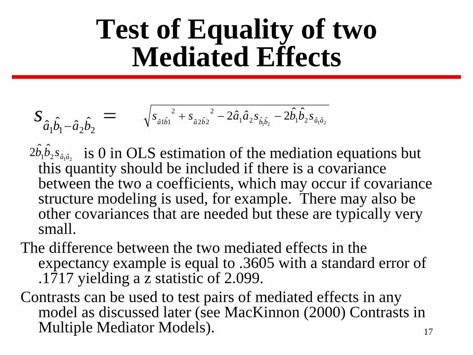
Test of Equality of two Mediated Effects

is 0 in OLS estimation of the mediation equations but this quantity should be included if there is a covariance between the two a coefficients, which may occur if covariance structure modeling is used, for example. There may also be other covariances that are needed but these are typically very small.

The difference between the two mediated effects in the expectancy example is equal to .3605 with a standard error of .1717 yielding a z statistic of 2.099.

Contrasts can be used to test pairs of mediated effects in any model as discussed later (see MacKinnon (2000) Contrasts in Multiple Mediator Models).

=− 2211

ˆˆˆˆ babas 2121ˆˆ21ˆˆ21

22ˆ2ˆ

21ˆ1ˆ

ˆˆ2ˆˆ2 aabbbaba sbbsaass −−+

21 ˆˆ21ˆˆ2 aasbb

17

Other Tests for Mediation in the Multiple Mediator Model

Product of coefficients will generalize to other models.

Causal StepsJoint SignificanceDifference in Coefficients

18

Baron & Kenny and Judd & Kenny, test for the Multiple Mediator Model

1. X is significantly related to Y.2. X must affect M1 and X must affect M2.3. M1 and M2 must affect Y after adjustment

for X.4. Must be nonsignificant for JK or must

be less than for BK.'c 'c

c

19

Limitations of BK and JK Steps: Multiple Mediator Model

1. Just investigates overall mediation; no way to look at specific mediated effects.

2. No significance testing of specific or total mediated effects. What if path from M1 to Y is statistically significant but M2 to Y is not? What if X to M1 is significant but X to M2 is not?

3. Requirement of a significant total effect is not necessary for the same reasons as for the single mediator case, e.g., inconsistent mediation effects.

20

Limitations of Joint Significance Causal Steps test

1. Could look at significance of two paths in each mediation relation.

2. But the total mediated effect is interesting too, not just each path in the specific mediated effect. Cumbersome to test significance of the total effect with a joint significance test, perhaps a null hypothesis of whether all four paths (in the two mediator model) are statistically significant.

21

Limitations of Difference in Coefficients Mediation Test

1. Provides a test of the overall mediated effect with and its standard error.

2. No clear way to get estimates of the specific mediated effects. Could test prediction of Y with just M1, then Y with just M2, and Y with both M1 and M2, and use the change in coefficients in some way to get an estimate of each specific mediated effect.

3. The method ignores the individual a paths which are important to investigate specific mediated effects.

'ˆˆ cc −

22

Product of Coefficients are #1

Product of coefficients tests generate more useful information are relatively easy to apply and provide estimates, standard errors, and confidence intervals.

Product of coefficients tests apply to complex models and are used throughout the course.

Hooray for the Product of Coefficients.

23

Inconsistent Mediation: Multiple Mediator Style

Inconsistent mediation models are models where at least one of the mediated effects and direct effects have different signs (see MacKinnon, Krull, & Lockwood 2000).

Same idea as in the single mediator case but it is easier to think of inconsistent mediation in the multiple mediator model because of opposing or iatrogenic effects. Iatrogenic means induced inadvertently by a physician or surgeon or by medical treatment or diagnostic procedures. 24


REASONS TO USE AAS

XM

PROGRAM

X Y


.573 (.105) .073 (.014)

-.181 (.056)

Mediated effect = .042Standard error = .011 25

Mediators of null effect of status on perceived sexual harassment

(Sheets & Braver,1999) Power

PerceptionsM1

X YSocial

Dominance

M2

+

Organizational Status

Harassment

+

-

0

+

26

Mediators of the competition effect (Murayama & Elliot, 2012)

Approach

GoalsM1

X YAvoidance Goals

M2

+

Competition Performance

+

-

0

+

27

Mediators of the null effect of age on typing (Salthouse, 1984)

Reaction

TimeM1

X YSkill

M2

+

Age Typing

Proficiency

+

+

0

-

28

Selection, Optimization, and Compensation Theory of Aging (Baltes, 1997)

A theory predicting inconsistent mediation.Selection - restriction of life to fewer domains of functioning.Optimization - selection of behaviors that enrich or augment basic reserves of focus on life course.Compensation - compensate for loss of capacity with other methods. Compensation implies opposing mediational processes for the effect of aging.

Baltes, P. B. (1997). On the incomplete architecture of human ontogeny: Selection, optimization, and compensation as foundation of developmental theory. American Psychologist, 52, 366–380. 29

Contrasts in Multiple Mediator Models

Multiple mediator models introduce more than one mediated effect for each dependent variable.Contrasts may used to compare pairs of effects or two groups of mediated effects.The direct effect may be included in contrasts also.Any combination of effects may be compared as long as all effects have the same dependent variable – makes scaling of all effects the same and thus they may be directly compared to one another.(MacKinnon, 2000)

30

Multiple Mediator Model of Intent to Use Anabolic Steroids

Group Intentions

Knowledge of the effects of AAS use

Team as inform-ation source

Perceived risks of AAS use

Reasons to use AAS

.236

2.42 (.258)

.149

.62 (.108)

.217

.52 (.061)

.168

.44 (.066)

-.083

-.02 (.006)

-.079

-.08 (.006)

-.265

-.25 (.024)

.155

.09 (.014)

.000

.001 (.056)

31

Summary of Multiple Mediators Remember the assumptions of the single mediator

model apply to the multiple mediator model. The additional variables address the omitted variable assumption. But other assumptions still apply.

Specificity of significant mediation paths improve interpretation.

The results from a multiple mediator model may shed light on the true underlying mechanisms but there are alternative explanations of results. Remember that the path relating the mediators to Y is correlational.

32

1

Mediation and Moderation Effects

ModerationModerators and Mediators TogetherWhen Mediation Differs by GroupBaseline by Treatment Interactions

2

Moderation Statements• Treatment effects differ for males and females.

• Program effects on tobacco use are greater for people who are more likely to believe positive consequences of tobacco use at baseline.

• A program works for middle school students but does not work for high school students.

• Program effects differ as a function of baseline measures of the outcome variable.

• Success of nicotine patch treatment differs depending onwhether person has a certain genetic disposition.

3

Definition of a Moderator (1)

• A moderator is a variable that affects the strength and/or form of the relation between X and Y

• Moderator variables determine for whom a treatment is effective when X represents assignment to a treatment group

• Moderator variables are often represented by the letter Z

4

Definition of a Moderator (2)

• A moderator variable (Z) is not intermediate in the causal sequence between X and Y, so it is not a mediator variable (M).

• Moderator effects are also called interaction effects, such that the relation between X and Y depends on a third variable, the moderator (Z).

5

Path Diagram of the Moderation Model for Individual Groups

c1X Y

c2X Y

Group 1

Group 2

Different regression coefficients predict Y from X in each group, indicating that the X-Y relation differs across the moderator

6

Path Diagram of the Moderation Model for Combined Groups

b1

b3

b2

X

XZ

YZ

A single interaction term, the product of X and Z, now

represents differences in the X-Y relation across Z

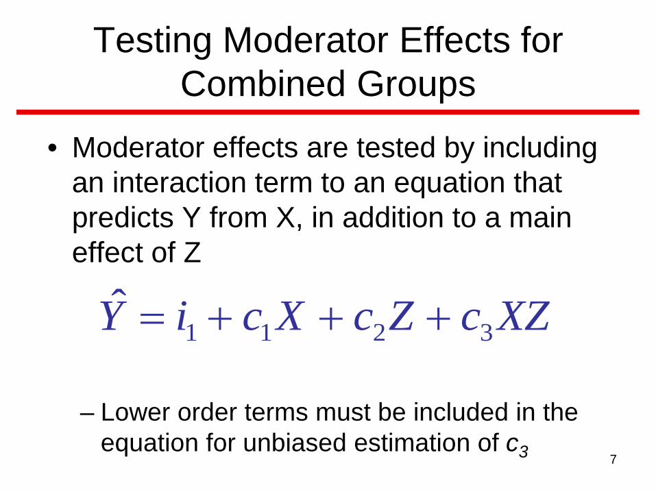
7

Testing Moderator Effects for Combined Groups

• Moderator effects are tested by including an interaction term to an equation that predicts Y from X, in addition to a main effect of Z

– Lower order terms must be included in the equation for unbiased estimation of c3

XZcZcXciY 3211ˆ +++=

8

Simple Slopes

• Graphing simple slopes shows how the effect of X on Y differs for Z = 0 and Z = 1

0

10

20

30

40

50

Control Program

X

Y

■ Z=0

▲ Z=1

9

Centering Terms

• Centering terms (subtracting mean scores on a variable from each observed score) is important in moderation analysis to reduce multicollinearity and to adequately interpret regression coefficients

• The interaction term in the general moderation model is the product of the centered X and centered Z variables

(see Aiken & West, 1991)

10

Why study both mediation and moderation effects?

• Both effects are important– Understand how manipulations achieve effects and identify

characteristics of participants and/or environment that moderate effectiveness of a manipulation.

• Streamline/improve manipulations by understanding for whom and/or under what conditions they operate.

• Can test hypotheses regarding the consistency and specificity of results across groups.

• Better target subgroups by understanding how they differentially respond to manipulations– Does a program differentially affect participants based on

level of risk?

11

Questions you can ask by Combining Mediation and

Moderation Models (1)1. “Is the mechanism by which a manipulation

achieves its effects the same across groups?”– Asks if the mediated effect differs across levels of a moderator

variable (MODERATION OF THE MEDIATED EFFECT)

2. “Is the reason an overall manipulation effect is moderated explained by a mediation process?”– Asks if an interaction effect can be explained by a mediating

mechanism (MEDIATION OF A MODERATOR EFFECT)

12

Questions you can ask by Combining Mediation and

Moderation Models (2)3. “Does the manipulation change the mediator

in the same way across groups?”– Asks if the action theory of the manipulation is the

same across levels of a moderator variable (TEST OF HOMOGENEITY IN THE a PATH)

4. “Is the mediating variable related in the same way to the outcome across groups?”

– Asks if the conceptual theory of the manipulation is the same across levels of a moderator variable (TEST OF HOMOGENEITY IN THE b PATH)

13

Moderators in and out of the Mediation Process

• Moderator in the mediation process, i.e., the mediating variable M or dependent variable Y, e.g., also larger effects for persons lower on the mediator or outcome.

• Moderator out of the mediation process, i.e., not X, M, or Y. There are different mediation relations at different values of the moderator, e.g., different effects for males and females.

14

The Interaction of X and M in the Single Mediator Model (Chapter 10)

• XM interaction test of whether the relation between M and Y differs across levels of X.

• Simple slopes and Simple Mediation Effects.• A Fourth-variable Effect where XM is the

fourth variable.

15

Three Mediation Equations

Y = i1+ c X + e1

Y = i2+ c’ X + b M + h XM + e2

M = i3+ a X + e3

16

Assumption of no XM Interaction

• An assumption of the single mediator model without the XM interaction is that the M to Y relation was the same across levels of X, i.e., the b path was equal across levels of X. – If the b path differs it means that the conceptual theory relation differs

at different values of X.– The assumption can be tested by including the XM interaction in the

model where both X and M predict Y. If it is nonsignificant, the evidence is that the b paths do not differ.

• There are cases where b is expected to differ– Example: a drug prevention program targets skills to deal with drug

offers so that the relation between offers and drug use is much less for participants receiving the program

17

The XM Interaction (Equation 10.3)

• The h coefficient represents whether the b path differs across levels of X (Judd & Kenny, 1981).

• If h is statistically significant it means there may be a more complicated form of mediation where the b path differs across groups.

22 ' ehXMbMXciY ++++=

18

Test of the XM Interaction for the Water Consumption Example

• h = .0299, sh = .1198, th = 0.25 so there is not evidence that the relation of M to Y differs across the two groups for the example described earlier.

22 ' ehXMbMXciY ++++=

19

Plot of the XM interaction for the Water Consumption Example

Relation of M to Y

1

2

3

4

+1 sd Mean -1 sdValue of M

Pred

icte

d Y X +1 sd

X MeanX -1 sd

20

Simple Mediation Effects #1• A significant XM interaction means that the b

path differs across levels of X. • The water consumption plot in the last slide

showed the different b value for +1SD, mean and -1SD values of X. These are simple slopes. Remember X was continuous.

• A simple mediation effect would be the value of ab at different values of X, e.g., the simple mediation effect at the mean.

• The standard error of the simple mediation effect uses the a coefficient and standard error and b coefficient and standard error--at a certain value of X.

21

Simple Mediation Effects #2• For a binary X, there are two simple slopes, e.g.,

treatment and control. For a continuous X, there are many simple slopes and simple mediated effects and a different mediated effect at the different values of X.

• The significance of the b path is obtained by centering the X variable at different values and the significance of b is obtained from the corresponding statistical analysis.

• If X is centered at zero, then the b path significance test is at an X value of 0.If X is centered so its average is 1SD above the mean then the significance of the b path is the value in the output. This can be done for any value of X to test simple slopes and simple mediation effects.

22

When XM interactions occur?

1. Measurement. The mediating variable means something different in the two groups. 2. Non-linear relation between M and Y. The X intervention changes the level of M so that the relation between M and Y in the program group differs. 3. Restriction of range. X changes M to a level where there is a ceiling or floor effect so the relation is not as large.4. Longitudinal. There is change in M in the experimental group but no change in the control group.5. Omitted Variable. There is an omitted variable that comes into play at different values of M.

23

Example XM interactions 1.• 1. Dietary intervention (X) teaches knowledge of healthy diet

(M) which is expected to improve diet. Without intervention, dietary behavior results from habit, not knowledge. Control group has a low relation between knowledge and diet behavior. In intervention group, the relation between knowledge and diet is stronger because participants learn about diet (Judd & Kenny, 1981).

• 2. Mindfulness intervention increases attention to pain. In the control group attention to pain increases experience of pain. In the intervention group, attention to pain reduces pain because of the mindfulness intervention.

24

Example XM interactions 2.• 3. Intervention (X) teaches social competence (M) to

reduce aggressiveness. For persons low on social competence, the program effect is much larger than for persons already high on social competence.

• 4. Intervention (X) increases self-efficacy to eat properly which improves diet (Y). For persons whose diet is already appropriate, the program does not have much of an effect.

25

Moderators of Mediation Relations as a Fourth variable, Z

• X, M, and Y are measured and a fourth variable Z, the moderator, is now included in the model. – There are many different types of relations in a model

that contains X, M, Y, and Z. • The moderator is usually a variable across which

mediation relations differ, not a variable that causes X, M, or Y, but it could also be a cause of these variables.

• Examples of moderators: (1) Stable: gender, age, race, (2) Individual Differences: SES, risk taking, impulsivity

26

Examining Mediation and Moderation for Individual Groups

• By testing the mediation model for different groups we can examine several possibilities:– Homogeneity of the Mediated Effect (Question 1)

– Homogeneity of Action Theory (Question 3)

– Homogeneity of Conceptual Theory (Question 4)

27

Homogeneity of Action Theory for Individual Groups

H0 : agroup1 – agroup2 = 0H1 : agroup1 – agroup2 ≠ 0

– Heterogeneous action theory corresponds to different a paths (i.e., the first link in the mediation model) across moderator-based groups

28

Testing Homogeneous Action Theory for Individual Groups

• A significance test for the effect is computed by taking the difference of the a paths across groups and dividing the estimate by a standard error of the difference:

2ˆ

2ˆ

21

21

ˆˆ

aa ssaa+

−

29

Homogeneity of Conceptual Theory for Individual Groups

H0 : bgroup1 – bgroup2 = 0H1 : bgroup1 – bgroup2 ≠ 0

– Heterogeneous conceptual theory corresponds to different b paths (i.e., the second link in the mediation model) across moderator-based groups

30

Testing Homogeneous Conceptual Theory for Individual Groups

• A significance test for the effect is computed by taking the difference of the b paths across groups and dividing the estimate by a standard error of the difference:

2ˆ

2ˆ

21

21

ˆˆ

bbss

bb+

−

31

Homogeneity of the Mediated Effect for Individual Groups

H0 : agroup1bgroup1 – agroup2bgroup2 = 0H1 : agroup1bgroup1 – agroup2bgroup2 ≠ 0

– A heterogeneous mediated effect corresponds to moderation of the mediated effect (has been called moderated mediation)

32

Path Model for Testing Homogeneity of Mediated Effect in Individual Groups

X M Yagroup1 bgroup1

c’group1GROUP 1

X M Yagroup2 bgroup2

c’group2

GROUP 2

Mediatedeffect:

agrp1bgrp1

Mediatedeffect:

agrp2bgrp2

33

Book Example for Mediation and Moderation for Individual Groups

• Chapter 3 Water Consumption example:– A variable Z was introduced into study, creating two

groups: • Group Z = 0: Normal Participants (Chapter 3)• Group Z = 1 Fit Participants (Chapter 10)

• Recall X = temperature, M = self-reported thirst, Y = water consumed.

• Do the two groups differ in how self-reported thirst mediates the relation of temperature on water consumption?

34

Book Example for Mediation and Moderation for Individual Groups

• There is not significant moderation of the mediated effect. That is, the mechanism by which temperature affects water consumption is the same across normal and fit participants.

• Note that assuming the two groups are independent, the standard error of this test is the pooled standard error of the mediated effect from each group.

76069.016096.005489.

26448.15272.

ˆˆˆˆ2

222

11

21

−=+−

=

+

−

baba

groupgroup

ss

baba

35

Examining Mediation and Moderation for Combined Groups

• As in the basic moderation model, moderator effects in the mediation model may be represented for combined groups

• There will be two equations for the combined group notation because there are two equations in the basic mediation model

• Interaction terms in the equations will now represent the group differences as with the basic moderation model

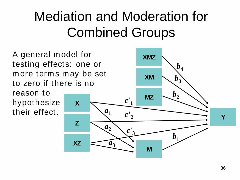
36

Mediation and Moderation for Combined Groups

b1

b2

b3

b4

a3

a2

a1

c'1

c’2

c'3

X

Z

XZM

MZ

XM

XMZ

Y

A general model for testing effects: one or more terms may be set to zero if there is no reason to hypothesize their effect.

37

Mediation in the General Model for Testing Mediation & Moderation

b1

b2

b3

b4

a3

a2

a1

c'1

c’2

c'3

X

Z

XZM

MZ

XM

XMZ

Y

38

Mediation and Moderation for Combined Groups Hypotheses (1)

• Test of homogenous action theory is now:

H0 : a3 = 0H1 : a3 ≠ 0

• (a3 = 0) is equivalent to (agroup1 – agroup2 = 0)when the moderator is dichotomous

39


• Test of homogenous conceptual theory is now:

H0 : b2 = 0H1 : b2 ≠ 0

• (b2 = 0) is equivalent to (bgroup1 – bgroup2 = 0)when the moderator is dichotomous

40


• Test of a homogenous mediated effect is more complicated to test

• Some argue that a joint significance test of a3 and b2 can provide evidence for moderation of the mediated effect

41

An Example XM interaction:Baseline by Treatment Interaction

• Mediation depends on the baseline measure of the mediating variable

• Program effects are often largest for persons with the lowest scores on the mediator at baseline

• Baseline levels of the mediator (M1) act as a moderator variable

• Two waves of data are needed for this design, such that X predicts M2 which predicts Y2, with M1 acting as a moderator of the relation

42

Baseline by Treatment Interaction Path Diagram (Morgan-Lopez, 2003)

X1

Y1

X 1M 1

Y 2

M 1

M 2

a 1

a 2

a 3

bc’1

c’2

c’3

c’4

43

Summary of Analyzing Mediation and Moderation Together

• Mediation and moderator effects can be analyzed simultaneously in the same model.

• Both mediation and moderation are important for investigating how programs work. Can test homogeneous action and conceptual theory across subgroups.

• Moderators can be inside or outside the mediation process.

• Models are available to test different effects of interest when jointly analyzing mediation and moderation.

1

Parallel, Sequential, and SEM Mediator Models (Chapters 6 and 7)

More detail on the two mediator model: a parallel

two mediator model and a sequential two mediator

model.

General SEM model for mediation.

Mplus demonstrations because it has capabilities for

estimating specific mediated effects.

2

MEDIATOR

M1

INDEPENDENT

VARIABLE

X

DEPENDENT

VARIABLE

Y

MEDIATOR

M2

c


= X + e1

Equation 5.1

cY

3

MEDIATOR

M1

INDEPENDENT

VARIABLE

X

DEPENDENT

VARIABLE

Y

MEDIATOR

M2

a1

a2

2. The independent variable is related to the potential mediators:

1 = 1X + e2, 2 = 2X + e3,

Equations 5.3 and 5.4

aa MM

4

MEDIATOR

M1

INDEPENDENT

VARIABLE

X

DEPENDENT

VARIABLE

Y

MEDIATOR

M2

a1

a2

b1

b2

c’

3. The mediators are related to the dependent variable controlling for

exposure to the independent variable:

= X + 1M1 + 2M2 + e6

Equation 5.2

'c bbY

5

Mediated effects = a1b1, a2b2

Standard error =

Total mediated effect= a1b1+ a2b2= c - c’

Direct effect= c’ Total effect= a1b1+ a2b2+c’=c




2 2 2 2

ii b i aia s b s

a1b1

2222

iaiibi sbsa

Mediation Effects

6

Mplus for the Two Mediator ModelDATA: File is 'E:\Med Course

2\Chap6_twomed.txtmultmedp2.txt';

Variable:

Names are X M1 M2 Y;

Usevariables are y M1 M2 x;

Analysis:

Model:

Y on M1 M2 X; Equation 5.2

M1 on X; Equation 5.3

M2 on X; Equation 5.4

M1 with M2; Covariance between the mediators

X; Variance of X

Model Indirect:

Y ind X;

Output:sampstat cinterval tech1 tech3;

7

MODEL INDIRECT :

Y IND X; TOTAL, TOTAL INDIRECT, SPECIFIC INDIRECT, AND DIRECT EFFECTS

Estimates S.E. Est./S.E.

Effects from X to Y

Total 0.708 0.169 4.187 Total effect of X on Y.

Total indirect 0.596 0.170 3.499 Total of both mediated effects.

Specific indirect

Y

M1

X 0.478 0.153 3.132 Specific Mediated Effect through M1.

Y

M2

X 0.118 0.083 1.409 Specific Mediated Effect through M2.

Direct

Y

X 0.112 0.197 0.570 Direct Effect.

8

Two Mediator Equations

111ˆˆ eXaM

222ˆˆ eXaM

32211ˆˆ'ˆˆ eMbMbXcY

9

Two Mediator Matrix Equation

3

2

1

2

1

2

1

21

2

1

'0

000

000

e

e

e

c

a

a

Y

M

M

bbY

M

M

10

Mplus Tech1 and Tech3

The covariance matrix among estimates in a model is useful to obtain standard errors of functions of coefficients such as the proportion mediated, ratio of mediated to direct effect and contrasts among mediator.

Mplus will print out the covariance among the estimates and the correlation among the estimates with the Tech3 command on the Output line.

To be exactly sure how the Tech3 matrices are set up, use the Tech1 command which gives the order of the variables in the Tech3 matrices.

11

PHLAME Two Mediator Model

• Firefighter study looked at mediators of the relation

between exposure to the TEAM (X) program and

participants’ BMI (Y) at posttest.

• Two mediators were hypothesized to be dietary support

(M1) and fruit & vegetable intake (M2)

XM1M2Y =

TEAM Dietary Support FV intake BMI

12

Two Mediators in a Sequence

X Y

M2M1

The mediated effect is ade.

ad e

1M = a0 + aX 2M = d0 + dM1 + fX

Y= e0 + eM2 + gM1 + c′X

f gc′

13

Two Mediators in a Sequence:

The PHLAME Example

a

de

f g

c′Team

Fruit/Veg

Intake

BMI

Dietary

Support

14

Two Mediators in a Sequence:

MPLUS Syntax for PHLAME Example

title: Sequential Multiple Mediator Example;

data: file is newmed.txt;

variable: names are dtst wght1 bmi1 whrat1… dietsup3 team mi;

usevariables are bmi2 total2 dietsup2 team;

missing are all (-99.000);

analysis: type = general missing h1;

bootstrap=1000;

model: bmi2 on total2 dietsup2 team;

total2 on dietsup2 team;

dietsup2 on team;

model indirect: bmi2 IND total2 dietsup2 team;

total2 IND dietsup2 team;

output: tech1 sampstat;

15

MPLUS Model Indirect Statements

for PHLAME ExampleTOTAL, TOTAL INDIRECT, SPECIFIC INDIRECT, AND DIRECT EFFECTS

Estimates S.E. Est./S.E.

Effects from TEAM to BMI2

Sum of indirect -0.013 0.010 -1.283

Specific indirect

BMI2

TOTAL2

DIETSUP2

TEAM -0.013 0.010 -1.283

Effects from TEAM to TOTAL2

Sum of indirect 0.197 0.084 2.347

Specific indirect

TOTAL2

DIETSUP2

TEAM 0.197 0.084 2.347

Mediation in Structural Equation Models

• Many models have multiple IVs, DVs, and/or mediators

• With more than one dependent variable, a more detailed modeling approach is required. Separate regression analyses will not longer be accurate, e.g., correlated dependent variables, measurement models, correlated error terms. The new method is called path analysis, structural equation modeling, or covariance structure modeling.

• Matrices are used to specify and estimate these models because matrices provide a way to organize all the relations in the model. The number and type of mediated effects are increased in these models. Matrix equations are used to find mediated effects and their standard errors.

16

17

Three Ways to Describe a Model

• Verbal Description: Translation of ideas often the

hardest part of SEM.

• Diagram: Amos, for example, takes a diagram as

input to the program, i.e., the model is specified

with a diagram.

• Equations: Can be used for all programs.

Equations may be regular regression equations or

the matrix representation of equations. With

complex models, the matrices provide a general

way to represent effects.

18

Model Specification

• Model specification includes:

• Specifying variables to be included in the model

• Specifying the number of latent variables, if any, to be modeled (no latent variables in Path Analysis)

• Specifying the relations between the variables

• Specifying constraints, etc.

Socioeconomic Status and Achievement

• Duncan et al. (1972) presented data on achievement that have been used to illustrate methodological developments in mediation. The data are from 3214, 35-44 year old males measured during the March of 1962 as part of a large survey of the civilian labor force.

• Occupational Changes in a Generation (OCG) Study.

• There are six variables: X1 father’s occupation, X2 father’s education, X3 number of siblings in the respondent’s family, Y1 respondent’s education, Y2 respondent’s occupational status, and Y3 respondent’s income.

• Many types of mediated effects focusing on parental effects on offspring.

19

Father

Occupation

X1

Father

Education

X2

No. of

Siblings

X3

Resp.

Education

h1

Resp.

Income

h3

Resp.

Occupation

h2

B32.0704

(.0045)

B214.3767

(.1202)

B31.1998

(.0364)

g23-.4631

(.1231)

g33-.0373

(.0314)

g13-.2281

(.0176)

g11.0385

(.0025)

g31.0114

(.0045)

g21.1352

(.0175)

g12.1707

(.0156)

g22.0490

(.1082)

g32.0712

(.0275)

20

Equations in the OCG Model

η1 = γ11ξ1 + γ12 ξ2 +γ13ξ3 + ζ1 (6.19)

η2 =β21η1 + γ21ξ 1 + γ22 ξ2 + γ23ξ3 + ζ2 (6.20)

η3 = β31η1 + β32η2 + γ31ξ1 + γ32 ξ2 +γ33ξ3 + ζ3 (6.21)

21

Father

Occupation

X1

Resp.

Education

h1

Resp.

Occupation

h2

B21

4.3767

(.1202)

g11

.0385

(.0025)

X1–>η1–> η2

γ11β21

(.0385) (4.3747) = .1685

sγ11β21 = Square Root[

(.0385)2 (.1202)2 + (4.3747)2

(.0025)2 ]=.0118

2 22 2ab b as a s b s

22

Father

Occupation

X1

Resp.

Education

h1

Resp.

Income

h3

Resp.

Occupation

h2

B32.0704

(.0045)

B214.3767

(.1202)

g11.0385

(.0025)

23

Father

Occupation

X1

Resp.

Education

h1

Resp.

Income

h3

Resp.

Occupation

h2

B32.0704

(.0045)

B214.3767

(.1202)

B31.1998

(.0364)

g11.0385

(.0025)

g21.1352

(.0175)

24

Mplus OCG ProgramTITLE: Chapter 6 Multiple Mediator Model Path Analysis with OCG Data

DATA:

Type is STD Correlation; *Reads in standard deviations and correlation matrix.

Ngroups=1;

Nobservations=3214;

File is Chap6_ocgexample.txt;

VARIABLE:*Note that mnemonic variable names are used.

Names are INC1961 OCC1962 EDUC NUMSIB FATHOCC FATHEDUC;

Usevariables are INC1961 OCC1962 EDUC NUMSIB FATHOCC FATHEDUC;

ANALYSIS:

Type is general;

Estimator is ML;

Iterations are 1000;

Convergence is 0.00005;

MODEL:

INC1961 on EDUC OCC1962 FATHEDUC NUMSIB FATHOCC;

EDUC on FATHOCC FATHEDUC NUMSIB;

OCC1962 on FATHOCC FATHEDUC NUMSIB EDUC;

MODEL INDIRECT:*Estimates Indirect Effects.

INC1961 ind EDUC FATHEDUC;

INC1961 ind FATHOCC;

OUTPUT:

sampstat mod standardized tech1 tech2;

25

Model Indirect for OCG Model TOTAL, TOTAL INDIRECT, SPECIFIC INDIRECT, AND DIRECT EFFECTS

Estimates S.E. Est./S.E. Std StdYX

Effects from FATHOCC to INC1961 *MODEL INDIRECT INC1961 IND FATHOCC;

Total 0.040 0.005 8.734 0.040 0.175

Total indirect 0.029 0.002 13.334 0.029 0.125

Specific indirect

INC1961

OCC1962

FATHOCC 0.010 0.001 6.930 0.010 0.041

INC1961

EDUC

FATHOCC 0.008 0.001 5.180 0.008 0.033

INC1961

OCC1962

EDUC

FATHOCC 0.012 0.001 10.561 0.012 0.051 *Three path mediated effect

Direct

INC1961

FATHOCC 0.011 0.004 2.535 0.011 0.049

Effects from FATHEDUC to INC1961 *MODEL INDIRECT INC1961 IND FATHEDUC;

Sum of indirect 0.034 0.007 4.912 0.034 0.024

Specific indirect

INC1961

EDUC

FATHEDUC 0.034 0.007 4.912 0.034 0.024

.

26

Summary of OCG Indirect Effects

27

Anabolic Steroid Book Example

X three measures of coach tolerance for steroids at

time 1. Higher means less coach tolerance.

M three measures of perceived severity of steroid use

at time 2. Higher means less perceived severity.

Y three measures of intentions to use steroids at time

3. Higher means more intentions to use.

Same mediation relations relating the now latent X, M,

and Y variables, X to M, M to Y, and X to Y.

N=54728

ATLAS Latent Variable Mediation Model

Not

Tolerant

Not

Severe

Intentions

a b

c’

X1 X2 X3

M1 M2 M3

Y1 Y2 Y3

ζ1

ζ2

29

Mplus for Latent Variable Mediation Model

TITLE: Chapter 7 Three Factor Latent Variable Model;

DATA: FILE IS chap7_exp1.txt; TYPE IS CORRELATION STD;

NGROUPS = 1; NOBSERVATIONS = 547;

VARIABLE: NAMES ARE coach1 coach2 coach3 severe1 severe2 severe3 intent1

intent2 intent3; USEVARIABLES ARE coach1 coach2 coach3 severe1 severe2

severe3 intent1 intent2 intent3;

ANALYSIS: TYPE IS GENERAL; ESTIMATOR IS ML;

Model: coach by coach1@1 coach2 coach3;

severe by severe1@1 severe2 severe3;

intent by intent1@1 intent2 intent3;

intent on severe coach;

severe on coach;

Model indirect:

intent ind coach;

OUTPUT: SAMPSTAT STANDARDIZED TECH1 TECH3; 30

Mplus Output for Three Latent Variable Mediation Model

MODEL RESULTS

Two-Tailed

Estimate S.E. Est./S.E. P-Value

COACH BY

COACH1 1.000 0.000 999.000 999.000

COACH2 1.746 0.251 6.962 0.000

COACH3 1.482 0.213 6.942 0.000

SEVERE BY

SEVERE1 1.000 0.000 999.000 999.000

SEVERE2 1.175 0.077 15.309 0.000

SEVERE3 1.269 0.082 15.455 0.000

INTENT BY

INTENT1 1.000 0.000 999.000 999.000

INTENT2 1.470 0.069 21.429 0.000

INTENT3 1.499 0.071 20.990 0.000

INTENT ON

SEVERE 0.266 0.048 5.540 0.000

COACH 0.001 0.068 0.021 0.984

SEVERE ON

COACH -0.415 0.093 -4.462 0.000

b

ˆ 'c

a

31

Mplus Output for Three Latent Variable Mediation Model

TOTAL, TOTAL INDIRECT, SPECIFIC INDIRECT, AND DIRECT EFFECTS

Estimates S.E. Est./S.E. Std StdYX

Effects from COACH to INTENT

Total -0.109 0.067 -1.623 -0.084 -0.084

Total indirect -0.110 0.031 -3.566 -0.085 -0.085

Specific indirect

INTENT

SEVERE

COACH -0.110 0.031 -3.566 -0.085 -0.085

Direct

INTENT

COACH 0.001 0.068 0.021 0.001 0.001

32

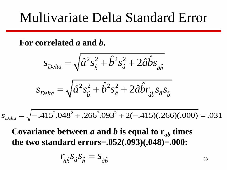
33

Multivariate Delta Standard Error

2 2 2 2

ˆ ˆˆ ˆ

ˆ ˆˆ ˆ2Delta ab abs a s b s abs

For correlated a and b.

2 2 2 2

ˆ ˆ ˆˆ ˆˆ

ˆ ˆˆ ˆ2Delta a ab ab bs a s b s abr s s

ˆ ˆ ˆˆˆ ˆaab b abr s s s

Covariance between a and b is equal to rab times

the two standard errors=.052(.093)(.048)=.000:

031.)000)(.266)(.415.(2093.266.048.415. 2222 Deltas

Summary

• Many potential mediated/indirect effects in path analysis

models.

• Can be complicated to calculate indirect effects and

standard errors of these effects. Formulas for effects and

standard errors can be applied to investigate mediation in

any model.

• Mplus Model INDIRECT command is very useful for the

calculation of indirect effects and their standard errors.

• Note that bootstrap and other methods can be used if the

raw data are available.34

1

Longitudinal Mediation Analysis (Chapter 8)

AssumptionsUnique Issues with Longitudinal RelationsTwo-wave Mediation ModelsThree or more wave Mediation Models

2

More on Temporal Order Assumption

• Assume temporal ordering is correct: X before M before Y.

• Assume that relations among X, M, and Y are at equilibrium so the observed relations are not solely due to when they are measured, i.e., if measured 1 hour later a different model would apply.

• Assume correct timing and spacing of measures to detect effects.

• But manipulations target specific times with many patterns of change over time.

3

Mediation is a Longitudinal Model• A mediator is a variable in a chain whereby an

independent variable causes the mediating variable which in turn causes the outcome variable—these are longitudinal relations. X, M, and Y in single mediator model imply longitudinal relations even if measured at the same time.

• For a single mediator model, temporal order for X is clear when it represents random assignment, but the temporal order of M and Y must be based on prior research or theory.

4

Timing of relations• When does X affect M or M affect Y? • Triggering, cascading, and other timing processes

(Tang & DeRubeis, 1999; Howe et al., 2002)• Tang & DeRubies (1999) found evidence that change

in therapy occurs within the first few sessions.• How are decisions made about timing? Not often

considered in research projects except with respect to when a manipulation is made and the easiest time for data collection.

• Timing is crucial for deciding when to collect longitudinal measures (Collins & Graham, 2003).

5

Cross-sectional mediation 1• Gollob & Reichardt (1991) describe three limitations of

cross-sectional mediation • 1. Takes time for effects to occur-may not be enough time

for X to affect M to affect Y if variables are measured at the same time.

• 2. Variables have effects on themselves-time 1 has an effect on time 2 etc.

• 3. Size of effect depends on time lag-effect 1 day apart is likely different from an effect 1 year apart.

• They specified a latent longitudinal model with prior measures as latent and lots of assumptions.

• Cross-section is a snapshot of relations

6

Cross-sectional mediation 2• Cole & Maxwell (2003) and Maxwell & Cole

(2007) demonstrate limitations with cross-sectional mediation relations as described by Gollob & Reichardt (1991).

• They present reasons for differences between cross-sectional and longitudinal mediation relations. Show that many studies use cross-sectional data to assess mediation.

• Maxwell & Cole (2007) present formulas for the bias if cross-sectional rather than longitudinal data are used to assess mediation.

7

Cross-sectional mediation 3• Cross-sectional X, M, and Y. Rank order of value

of X is associated with rank order of value of M which is associated with the rank order of value of Y.

• Two-wave X, M, and Y. Rank order of change in X is associated with rank order of change in M which is associated with the rank order of change in Y.

• Rank Order of the value of M is different than change in M. Relations among change in variables seem more compelling than relations among rank order of variables.

8

Cross-sectional models: Summary

• Models are often cross-sectional. • These models assume that a system has reached an

equilibrium so observed relations are not just due to the particular point of observation.

• But systems may be dynamic and change over time in complicated ways.

• Meaning of cross-sectional relations (relation between rank order of level) is different from longitudinal relations (relation of rank order of change).

• Cross-sectional mediation may differ in many ways from longitudinal mediation (Cole & Maxwell, 2003; Gollob & Reichardt 1991).

9

Does the study of mediation exclude cross-sectional data?

• Cross-sectional information is often used to infer relations in fields such as geography and astronomy and by detectives, physicians, and historians.

• Some cases where cross-sectional relations are more important than longitudinal change, e.g., legislator basing funding decisions based on change or level of a problem; school funding based on level or change in achievement.

10

Are there variables that represent changes over time when measured

once? • Age of onset: Started regular smoking at age 15.

Date of first arrest. • Drug use last week, exercise last month. • X measured at the first wave, M measured at the

second wave, and Y measured at the third wave. • Others?

11

Benefits of Longitudinal Data

• Time-ordering of X to M to Y is investigated. Can shed light on whether changes in M precede changes in Y.

• Both cross-sectional and longitudinal relations can be examined.

• Removes some alternative explanations of effects, e.g., effects of static variables can be removed.

12

What if repeated measures of X, M, and Y are available?

• Measures of X, M, and Y at two time points allow for several options, difference score, ANCOVA, residualized change score, relative change…

• Measures of X, M, and Y at three or more time points allow for many alternative longitudinal models.

• For many examples in this class, X is measured once and represents random assignment of participants to one of two groups.

13

Stability, Stationarity, and Equilibrium

• Stability-the extent to which the mean of a measure is the same across time. There are different kinds of stability (Wohlwill, 1973).

• Stationarity-the extent to which relations among variables are the same across time.

• Equilibrium-the extent to which a system has stabilized so that the relations examined are the same over time.

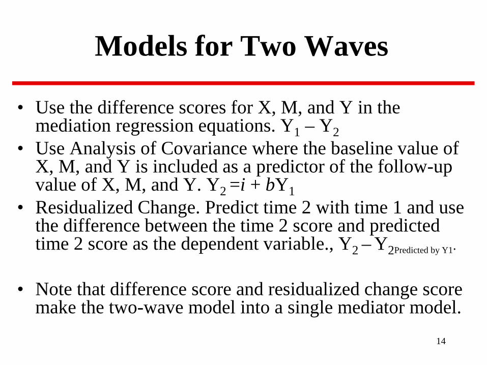
14

Models for Two Waves

• Use the difference scores for X, M, and Y in the mediation regression equations. Y1 – Y2

• Use Analysis of Covariance where the baseline value of X, M, and Y is included as a predictor of the follow-up value of X, M, and Y. Y2 =i + bY1

• Residualized Change. Predict time 2 with time 1 and use the difference between the time 2 score and predicted time 2 score as the dependent variable., Y2 – Y2Predicted by Y1.

• Note that difference score and residualized change score make the two-wave model into a single mediator model.

15

Reliability of the Difference score

• Cronbach & Furby (1970) difference scores are unreliable because the difference is just error.

• Rogosa (1998) lack of change is the explanation of low reliability. • Singer and Willett (2003) reliability of change is different than

reliability of a measure.Reliability of test.7 .8 .9

r,Time1,Time2.5 .4 .6 .8.6 .25 .5 .75.7 .00 .33 .67.8 .00 .50.9 .00

16

ANCOVA vs. Residualized Change Scores

• Theoretically the residualized change score approach is similar to ANCOVA since both analyses adjust for pretest measurement. For mediation the residualized change score does not account for baseline relation between M and Y.

• The statistical adjustment that generates the residuals in the residualized change score method uses the total regression coefficient for Y on X (that is, the regression coefficient of Y on X across all cases, ignoring group membership), whereas ANCOVA adjustment is based on the regressions of Y on X within each group pooled across groups, the pooled within class regression coefficientof Y on X.

• As a result, if there is no baseline imbalance between groups, ANCOVA and residualized change scores produce similar results. However if the groups differ at baseline, then residualized change scores can lead to an underestimated treatment effect. For mediation analysis ANCOVA is better because it includes the relation between M and Y at baseline.

17

Two-wave Longitudinal Model

BASELINEOUTCOME

BASELINEMEDIATOR

POST-TESTOUTCOME

POST-TESTMEDIATOR

PROGRAM

Mediated effect=a4b5Direct effect = c’3

b1

c’3a4

b5

b2

18

Summary of Two-Wave Models

• Difference score versus ANCOVA models. Randomized X then ANCOVA is best. But there are other measures. If there is a difference in the results between the two models, check for baseline differences.

• Difference score and residualized change measures are useful because they transform two measures to one measure, i.e., the difference score combines the time 1 mediator and time 2 mediator so all the models that we have discussed in this course so far can be applied.

• Meaning of mediation with the different models differ: Correlated change scores, correlated adjusted time 2 scores. Note issue of Lord’s paradox for the M to Y relation because M is not randomized.

• ANCOVA is generally the best approach because it models all the information from two waves of data.

• Models with two waves are half-longitudinal because some relations are cross-sectional but Cole and Maxwell suggest using a from X1 to M2 and b from M1 to Y2.

• More options with more waves of data. More complexity too though.

19

Models for Three or More Waves

Autoregressive Models Latent Growth Curve Models (LGM)Latent Change Score Models (LCS)Autoregressive and Latent Growth Curve

Models (ALT)Differential Equation Models (DEM)

20

1Χ 3Χ2Χ1b 2b

2ε 3ε

2123

22

21

3223

2112

,,,, bb

XbXXbX

x εε σσσ

ε

ε

+=

+=

Autoregressive (Jöreskog, 1974)

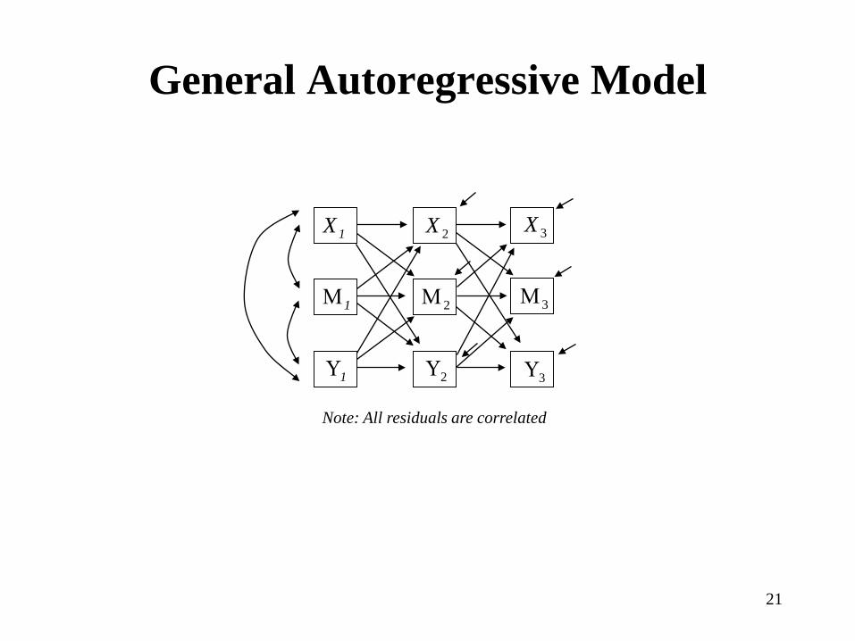
21

General Autoregressive Model

1Υ

1Μ

1X

2Υ

2Μ

2X

3Υ

3Μ

3X

Note: All residuals are correlated

22

Autoregressive Model with Time-Ordered Mediation, Cole & Maxwell (2003)

1Υ

1Μ

1X

2Υ

2Μ

2X

3Υ

3Μ

3X

2b

2c′

1s

2a1a

2s

1s

1c′2s

3s 3s

1b

Note: All residuals are correlated

23

Autoregressive Model with Time-Ordered Mediation (MacKinnon 1994, 2008)

1Υ

1Μ

X

2Υ

2Μ

3Υ

3Μ2b

2c′1a

2s1c′

2s

3s 3s

1b

Note: Residuals at the same time are correlated

24

Autoregressive Model with Contemporaneous Effects for M to Y (MacKinnon 2008; Marsh 1993)

1Υ

1Μ

X

2Υ

2Μ

3Υ

3Μ2b

2c′1a

2s1c′

2s

3s 3s

1b

Note: Residuals at the same time are correlated

2a

25

Autoregressive Models• Many mediated effects. Standard error of the sum of

(or any function) the indirect effects can be derived with the multivariate delta method, e.g., for the Cole and Maxwell (2003) overall indirect effect standard error on page 564.

• Model does not allow for random effects for individual change and does not include modeling of means. Change in growth of means is an important aspect of longitudinal data.

Latent Growth Model (LGM)• LGM model change over time by estimating an intercept

and slope for change in variables. These models can be used to investigate mediation by estimating change over time for the mediator and change over time for the outcome. The relation between the change in the mediator and change in the outcome is represented by the b path (Cheong et al. 2003).

• The causal direction of correlated change is ambiguous. Another LGM estimates change in the mediator at earlier time points and relates to change in the outcome at later time points providing more evidence for temporal precedence of the mediator.

26

Latent Growth Model (LGM)I S

Y1 Y2 Y3

1 11

1 2

ε1 ε2 ε3

Meredith & Tisak (1990)

MeansSIYSIYSIY

ISSI ,,,,,,

210

2222233

22

11

321ρσσσσσ

εεε

εεε

++=++=++=

27

1X 2X 3X

1Μ 2Μ 3Μ

1Υ 2Υ 3Υ

Xi

ms

Xsyi ys

mi

Latent Growth Curve Mediation Model

a

b

1c

Cheong et al., 2003

1 1

1

1

1 1

1 1 1

1

1

1 2

2

2

28

29

X

1Μ 2Μ 3Μ

1Υ 2Υ 3Υms

yi ys

mi

Latent Growth Curve

b'c

a

Nutrit1 Nutrit2 Nutrit3 Nutrit5

11 1

1 11

Program

PerIn1 PerIn2 PerIn3 PerIn5

1 11

0

11

PerIn6PerIn4

1

1

1

1

Nutrit6Nutrit4

11

10

η2

η3 η4

η1

1

1

a

c’b

a

c’b

Nutrit3 Nutrit5

11 11

Program

PerIn1 PerIn2 PerIn3

1

1

0

1 1

Nutrit6Nutrit4

11

10

η2

η3 η4

η1

1

1

31

Latent Change Score Models• LCS parameterize models by fixing parameters so

that change between adjacent waves is analyzed.• Really a special case of latent growth curve

modeling but with growth between adjacent waves.• More complicated change over time can be made by

picking different coefficients and second order factors.

• Promising model not often used for mediation analysis.

32

9/27/2016 D.P. MacKinnon

Latent Change Score (LCS)Two Waves McArdle (2001)

β1

D1

1

1

X1 X2

2 1 1

2 1 1

2 1 1

1 1 1 2

2 21 2 1

(1) (1)(1)

, ,x

X X DX X DX X DD B X

ε

ε

σ σ β

= +− =− == +

ε2

0

Latent Change Score (LCS) McArdle (2001)

ε2 ε3

β1

D2

β2

D1

1

1

X1 X2 X3

1

1

MeansXBDXBD

DXXDXX

x ,,,,, 2123

22

21

222

111

3223

2112

ββσσσ

εε

εε

==

++=++=

Latent Change Score Mediation Model

3X1X 2X

1X 3X2X

3Y 2Y 3Y

1M

2M

3M

x∆

1Y 2Y 3Y

x∆ 1M

2M

3M

M∆

M∆

Y∆ Y∆

1 1 1

11

11

1

1

1

1

1

1

1 1

1

1

1

1a

2a

1b2b

3a

3b

1c′ 2c′ 3c′

Latent Change Score Mediation Model Single X

3Y 2Y 3Y

1M

2M

3M

1Y 2Y 3Y

1M

2M

3M

M∆

M∆

Y∆ Y∆

1

1

1

1

1

1

1 1

1

1

1

1a

2a

1b2b

3b

1c′ 2c′

X

36

37

Longitudinal models for a steroid prevention project (ATLAS)

• Adolescents Teaching and Learning to Avoid Steroids (ATLAS). Randomized high school football teams in Oregon and Washington to receive the steroid prevention program or an information only group. Just individual data here.

• Measured the same persons over repeated occasions. Here we will look at four repeated measures. The dependent variable is intentions to use steroids.

• Linn Goldberg (OHSU) principal investigator. For more on the program see Goldberg et al. (1996) and for mediation see MacKinnon et al., (2001).

• Program delivered after baseline measurement. In general, timing of the mediators should be relatively quick for knowledge and beliefs measures. It may take longer for norms measures. Four waves of measurement for the models studied.

38

Analysis decisions

• LGM model, slope coded as 0 1 * 1 where * indicates a free parameter. Note that there was a booster after the 3rd measurement. If the model was not identified, then loadings were 0 2.5 * 14.5 to represent the months from baseline. All LGM models had RMSEA lower than .041 (lowest .019).

• Autoregressive model. Tested for stationarity in the aand b paths. Stationarity observed more often for b paths and less often for a paths, as expected. All RMSEAs lower than .088 (lowest was .068).

39

LGM and Autoregressive mediation effects

Mediator LGM Autoregressiveab(se) z a1b2(se) z a2b3(se) z

Knowledge -.28(.12) -4.88 -.08(.02) -4.90 -.03(.04) -0.48Coach Tol -.11(.05) -2.27 -.02(.01) -3.24 -.00(.00) -0.37Team as info -.21(.06) -3.42 -.04(.02) -3.30 .01(.01) 0.78Peer as info -.12(.05) -2.43 -.04(.01)-2.30 -.01(.00) -1.61Reasons not use -.12(.04) -2.98 -.02(.01) -3.01 .00(.00) 0.61Normative bel -.12(.07) -1.64 -.00(.00) -0.14 -.01(.01) -0.98

40

Measurement• Does the measure have the same meaning at each

wave? So it is possible that the system is stationary and stable but the measurement of the construct changes.

• Multiple indicator latent variable models are ideal. • Important to consider measurement of constructs at

each wave and measurement of change over time separately.

41

X, M, and Y may differ over time• X, M, and Y at an earlier developmental stage may differ

from X, M, and Y at a later stage. For example social norms may be important mediators of drug use prevention in middle school but positive alcohol expectancies may be important mediators for programs targeted at the transition from high school to college. Onset may be important for 13 year olds and heavy use may be important for 21 year olds. Intervention to change expectancies for 13 year olds may differ from expectancy interventions for 21 year olds.

• Many manipulations have an initial program and booster sessions so that even X differs over time, e.g., adaptive interventions.

42

Transitions as Critical Periods• Transitions are important, e.g., home to elementary school,

elementary to high school, high school to workforce/college. There are many aspects to these transitions including environmental, biological, social, and family changes.

• For example, interventions to reduce aggressive behavior from home to elementary school may focus on improving educational achievement while interventions to reduce aggressive behavior for the transition from middle to high school may focus conflict resolution and self-control.

43

Types of change over time• Change in X, M, and Y and also relations between change

in X on M and change in M on Y.• Cumulative: There may be cumulative effects such that

more M yields more Y. • Threshold: Once a mediator gets to a certain level, then it

will change Y.• Cascading: Once a proximal mediator changes it changes a

more distal mediator and finally an outcome variable.• Phase shift: Once a level of a mediator is reached, the

individual changes to a new level, e.g., learning a concept in algebra.

• The types of changes may differ over time.

44

Type of change may differ for X to M and M to Y

• Both the X to M and M to Y relations may be the same, e.g., linear cumulative change for X to M and M to Y. Often linear change is assumed for both.

• Effects of X on M may differ from M on Y. A cumulative change in the mediator may trigger change in Y.

• The change in X to M may lead to a phase shift or new stage which then leads to a stage shift in M to Y.

• Many different possibilities requiring detailed modeling both to describe these relations and then confirmatory models for the two parts of the mediation relation.

45

Sleeper Mediation Effects• Effects on mediators may have beneficial effects later. For

example an intervention to increase calcium consumption among teenage women may not yield beneficial effects on osteoporosis until much later.

• Interventions to improve educational achievement in elementary school may reduce problems in young adulthood.

• Social competence skills learned in elementary school may reduce violence as adults.

• Norm change to prevent gateway drug use may reduce heavy use later.

46

Correspondence between Measurement and Population Change

• Match between theoretical population model and timing of measures is crucial.

• Many waves of data collection do not ensure correct longitudinal modeling.

47

Population

Sample

X

M1 M2 M3

Y1 Y2 Y3

a

b

X

M1 M2 M3

Y1 Y2 Y3

M4 M5

Y4 Y5

a

b

48

Population

Sample

X

M1 M2 M3

Y1 Y2 Y3

M4 M5

Y4 Y5

a

b

X

M1

Y1

M5

Y5

a

b

49

Population

Sample

X

M1

Y1

M5

Y5

a

b

X

M1 M2 M3

Y1 Y2 Y3

M4 M5

Y4 Y5

a

b

50

Population

Sample

X

M1

Y1

M4 M5

Y4 Y5

a

b

X

M1 M2 M3

Y1 Y2 Y3

M4 M5

Y4 Y5

a

b

51

Summary• Longitudinal data provide more information. • Many alternative models that provide different

information about mediation effects.• Often requires an iterative process to model

longitudinal data.• Perhaps estimate all models on the same data and

compare results. So far different models lead to comparable conclusions.

• Need examples of applying the models to real data.

1

Mediation Special Topics

• Causal Mediation Analysis• Meta-analysis and data synthesis.• Categorical Variables• Multilevel Mediation Models• Bayesian mediation analysis.

Causal Inference in Mediation (Chapter 13)

• Assumptions of true causal relations and self-contained/comprehensive model for regression analysis for mediation.

• Blalock’s (1979) presidential address states that about 50 variables are involved in sociological phenomenon and Weinstein’s comprehensive versus limited health psychology models. How many variables are relevant in your research area?

• Problem with mediation analysis because M is not randomly assigned but is self-selected.

• Causal inference for mediation is an active research area (Frangakis & Rubin, 2002; Pearl, 2001; Pearl, 2009).2

3

Counterfactual/ Potential Outcome Models

• Most modern causal inference approaches are based on a counterfactual or potential outcome model.

• In these models, all the possible counterfactual and actual conditions of an experiment are considered and the statistical model is based on all these possible or potential conditions.

• The Marginal Structural Model is the regression model for these counterfactual and actual conditions. It differs from the usual regression model because it is based on potential outcomes.

• Natural and Controlled Effects.

4

Randomized Two Group Design

• Ideally we need the same individual in both the treatment and control conditions at the same time. Units (individual level) usually have observed data for one of two conditions but not the other—the fundamental problem of causal inference (Holland, 1986).

• Randomization of a large number of persons solves the fundamental problem of causal inference. The average in each group can be compared and is an estimator of a causal effect. It is called an average causal effect (ACE).

Why b and c’ Do Not Reflect a Causal Relation

• Because M is not under experimental control, b and c’ do not necessarily represent causal effects. M is both a dependent and independent variable.

• Need: The relation between M and Y for participants in the treatment group if they were in the control group; the relation between M and Y for control participants if they instead were in the treatment group. Coefficients b and c’ are not Average Causal Effects, because the counterfactuals for these relations are complicated because M is not randomly assigned.

5

Confounders of Mediation Relations

MEDIATOR

M


X Y

DEPENDENT VARIABLE

a

True model needs d1,d2, d3, d4, otherwise coefficients are confounded.

b

c’

Confounder of X to M

Relation

Confounder of M to Y

Relation

d3

d4

d2

d1

6

Sensitivity Analysis for Confounding

• How will results change with confounding of the M to Y relation, e.g. when X is randomized?

• VanderWeele (2010), confounder effect on Y and difference in proportions of the confounder between groups at level of M.

• Imai et al. (2010), confounder effect as the correlation between error terms.

• Adaptation of Left Out Variables Error (LOVE; Mauro, 1990) based on the correlation of a confounder with Y and the correlation of a confounder with M.

• See Cox et al., 2014, Evaluation Review.

7

Statistical Methods for Confounding

• Statistical approaches to improve causal inference from a mediation study. A way to deal with omitted variable bias.

1) Instrumental Variable Methods2) Principal Stratification3) Inverse Probability Weighting4) G-estimation

• Active area of research (MacKinnon & Pirlott, 2015, Personality and Social Psychology Review)…

8

9

Inverse Probability Weighting• Method to adjust results for confounders.• Assumes no unmeasured confounding.• Weights observations as a way to deal with

confounding, missing data etc. • Here weights are used to adjust for confounding of

the M to Y relation when R is randomized.• Marginal treatment effect under ignorability.

See Robins, Hernan, & Brumbeck (2000) and also Coffman (2011).Weighting has a long history starting in sampling (Horvitz & Thompson, 1952).

10

IPW is a General Procedure• Can be used to adjust for confounders, lack of randomization,

missing data, longitudinal data.• Can be used for models with many variables but need a

model to predict each variable, e.g., if X is not randomized, fit a propensity model for X and also M and conduct weighted analysis for M and Y.

• No unmeasured confounders assumption is likely better than no adjustment at all?

• Possible that adjustment would increase or decrease estimates based on weights.

• Weights can be unstable so there is research on different weighting methods (Cole & Hernan, 2008).

Design Approaches to Improving Causal Inference

• Statistical mediation analysis answers the following question, “How does a researcher use measures of the hypothetical intervening process to increase the amount of information from a research study?”

• Another question is, “What is the best next study or studies to conduct after a statistical mediation analysis to test mediation theory.”

1. Designs to address Consistency of the mediation relation.2. Designs to address Specificity of the mediation relation.

MacKinnon, 2008; MacKinnon & Pirlott, 2012 related to Hill’s (1971) considerations. Also SMART designs (Almiral et al., 2014)

11

12

(1) Consistency Mediation Designs• Consistency designs replicate mediation relations in new

settings, groups, species (animals, humans), and times.

• Consistency designs also replicate mediation relations with alternative manipulations (X), alternative measures of the same mediator (M), and other related dependent measures (Y).

• Overall, consistency designs provide evidence that the mediation relation is consistently observed across many domains and variables.

13

(2) Specificity Mediation Designs• Evidence for specificity of a mediation relation is obtained

by comparing between groups (or variables) to demonstrate that the mediation relation is present in the predicted groups (or variables) but not present in other groups (or variables).

• Specificity designs demonstrate that mediation relations can be changed by different manipulations (X), mediation relations are observed for some mediators (M) but not others, and mediation is observed for some dependent measures (Y) but not others in a way that demonstrates a pattern of results consistent mediation theory.

14

Blockage Specificity Designs• The goal of blockage designs is to test a mediation relation

with a manipulation that blocks the mediator from operating.

• For example, let’s say that an exercise program appears to reduce depression by increasing endorphin levels -- the hypothesized mediator. A blockage manipulation would administer a drug to prevent endorphin production so that persons receiving the exercise program would no longer experience reduced depression if the endorphin level is the mediator.

15

Enhancement Specificity Designs

• The goal of enhancement designs is to test interventions that enhance the effects of a hypothesized mediator.

• For example, let’s say that a treatment program improves abstinence by increasing social support. An enhancement design would include a group where social support is increased even more to demonstrate a larger effect on abstinence. Social support may be increased by more sessions with counselors, increasing exposure non addicted friends and family etc. in addition to the typical program.

Causal Mediation Summary

• Causal inference in mediation is challenging because M is not randomized.

• Can look at how effects would change for different confounder values.

• Can include measures of confounding variables in the statistical analysis.

• Experimental approaches to improving causal inference.

• Active research area with more to come. 16

17

Mediation for Integrated Data Analysis and Meta-Analysis

• Methods to combine information across research studies.• Estimates for X to M and M to Y relations.• Relation of M to Y is more problematic because M is not

randomized so relation between M and Y is correlational as it is for the single mediator model.

• Mediator constructs may differ across studies. Even if it is the same construct, measurement may differ. Weakness or a strength? Strengths: use as estimates of different aspects of a random process, measurement facets, Bayesian update estimates with each new study.

18

Mediation with a Categorical Dependent Variable (Chapter 11)

A dependent variable is often binary such as whether a person litters or not, used a condom or not, dead or alive, diseased or not, or divorced or not. Counts of events.

In this case, Poisson, logistic or probit regression is the method of choice because of violation of assumptions if ordinary least squares regression is used.

Estimates of the mediated effect using logistic and probit regression can be distorted using conventional procedures.

Here binary or continuous X, continuous M, and binary Y is described in detail (Chapter 11).

MacKinnon 2008; MacKinnon et al., Clinical Trials (2007)and MacKinnon et al., under revision.

19

Why ab and c-c′ are not equal in Logistic and Probit Regression…

• The two estimators, ab and c-c′ are not identical in logistic or probit regression because, unlike ordinary least squares regression where the residual variance varies across equations, in logistic regression the residual variance is fixed to equal π2/3 (MacKinnon & Dwyer, 1993). So the logistic regression coefficients are a function of the relations among variables and the fixed value of the residual variance.

• There are solutions if you want ab and c-c′ to be close. • Or just focus on ab and its standard error to make

confidence intervals or use Rmediation or the bootstrap.

20

Options for Categorical M and Y #1• Can just use product of coefficient methods with Rmediation

or bootstrap.

• Or you could use Mplus which standardizes across equations. Mplus also allows for path analysis models with combinations of categorical and continuous variables.

• Sample size requirements are larger for binary dependent variable than for continuous dependent variable.

• With logistic or probit regression, c-c’ does not always equal ab. Can standardize values to make c and c’ in the same metric so the c-c’ method is comparable to ab.

21

Options for Categorical M and Y #2Traditional and potential outcome approach to mediation

coincide for linear models and log-linear models.

For non-linear models with interactions, methods based on the counterfactual model may yield different results.

If you are using nonlinear models with interactions you can use the SAS and SPSS macros described in Valeri & VanderWeele (2012) to investigate how results may differ. Or you could use Imai et al.’s R program. Mplus with the Model Constraint command will work and counterfactual quantities is estimated in Mplus Version 7.2.

22

Multilevel Mediation (Chapter 9)

MediationMultilevel data as a nuisance and an opportunityMediation in Multilevel ModelsGroups, schools, classes, clinics, cities, states….and also individuals.Ecological and Atomistic Fallacies

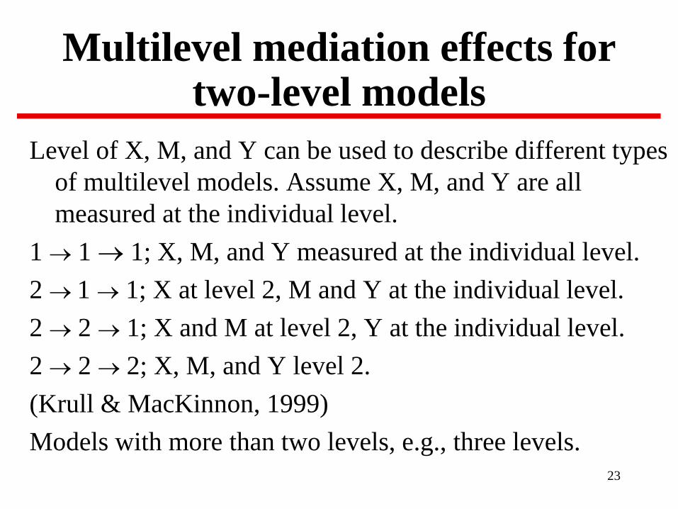
23

Multilevel mediation effects for two-level models

Level of X, M, and Y can be used to describe different types of multilevel models. Assume X, M, and Y are all measured at the individual level.

1 → 1 → 1; X, M, and Y measured at the individual level.2 → 1 → 1; X at level 2, M and Y at the individual level.2 → 2 → 1; X and M at level 2, Y at the individual level.2 → 2 → 2; X, M, and Y level 2.(Krull & MacKinnon, 1999)Models with more than two levels, e.g., three levels.

24

Multilevel mediation effects for three-level models

3 → 2 → 1; X (Schools), M (Classroom Observations), and Y (Individuals).

3 → 2 → 1; X (Schools), M (Person Norms), Y (Repeated Measures).

1 → 1 → 1; X, M, and Y measured at the individual level but the data have a three level structure, e.g., Individuals X, M, and Y within schools

See Preacher, K. J. (2011). Multilevel SEM strategies for evaluating mediation in three-level data. Multivariate Behavioral Research, 46, 691-731, and Pituch, K. A., Murphy, D. L., & Tate, R. L. (2010). Three-level models for indirect effects in school- and class-randomized experiments in education. Journal of Experimental Education, 78, 60-95.

Four-level, Five-level,…

25

Mediated Effects at Different LevelsMediated effects at group and individual level are possible

(MacKinnon, 2008).Controversy about individual level mediated effects when X

is at a higher level. For example in the 2 -1- 1 model, X is delivered at Level 2 and the M to Y relation is at Level 1. Does it make sense to consider this mediated effect at the individual level? It does not when only considering the data measured. But the population mediated effect is the intervention changing individuals even when X is at Level 2.

See Pituch, K.A., & Stapleton, L. M. (2012). Distinguishing between cross- and cluster-level mediation processes in the cluster randomized trial. Sociological Methods and Research, 41, 630-670.

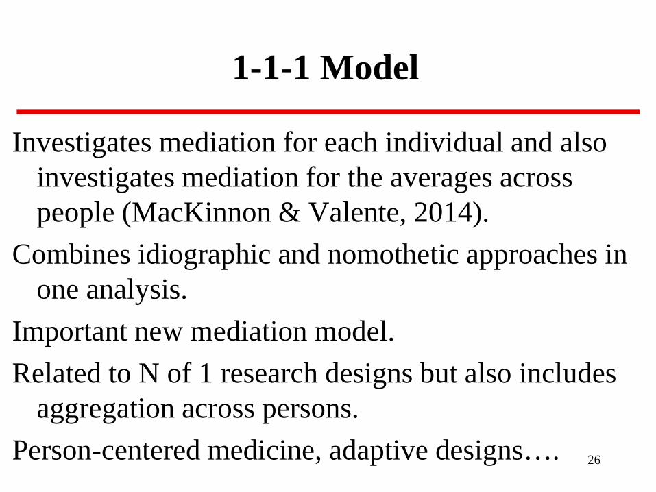
26

1-1-1 Model

Investigates mediation for each individual and also investigates mediation for the averages across people (MacKinnon & Valente, 2014).

Combines idiographic and nomothetic approaches in one analysis.

Important new mediation model. Related to N of 1 research designs but also includes

aggregation across persons. Person-centered medicine, adaptive designs….

27

1-1-1 Model Key Idea

There is a mediated effect for each individual and there is a variance of this mediated effect across individuals.

There is also an average mediated effect that combines information from each individual to compute the average mediated effect. This average mediated effect has more power and is usually the mediated effect of interest.

28

1-1-1 Figure

29

Multilevel Structural Equation Modeling (MSEM)

1. Allows for measurement models for constructs to accommodate measurement error.

2. General model that allows for simultaneous estimation of model coefficients, e.g., mediation models, more complex models.

3. Some fit indices, estimation strategies available in SEM can be applied to multilevel data.

Software now available and growing Mplus (Muthen & Muthen, 2001), GLLAMM (Rabe-Hesketh et al., 2004)

30

More information on MSEMMplus www.statmodel.comGLLAMM www.gllamm.org EQS http://www.mvsoft.com/products.htmLisrel http://www.ssicentral.com/lisrel/HLM http://www.ssicentral.com/hlm/UCLA mplus information http://www.ats.ucla.edu/mplusMlwin http://www.bristol.ac.uk/cmm/software/mlwin/Joop Hox’s homepage: http://www/joophox.netKris Preacher’s Mplus program examples: http://www.quantpsy.org/pubs/syntax_appendix_081311.pdf

http://www.statmodel.com/

http://www.ssicentral.com/lisrel/

http://www.ats.ucla.edu/mplus

http://www/joophox.net

http://www.quantpsy.org/pubs/syntax_appendix_081311.pdf

31

Multilevel SummaryTwo views of multilevel data: (1) a nuisance in the

statistical analysis and (2) an opportunity to investigate effects at different levels.

New Mplus version allows for estimation of many different models including random a and b effects using MSEM.

Can have very complicated models with many levels and potential mediation across and between levels.

Need applications to real data. Need methods work for information on statistical testing….

Bayesian Mediation Analysis: Fixed versus Random parameters

In frequentist statistics, parameters are fixed and unknown; we find point estimates and/or confidence intervals for parameters. The data are random.p-value=P(data|H0)

In Bayesian statistics, parameters are random and the data are fixed. We find point estimates (usually the mean or median of the posterior distribution) or probability intervals for the parameters.Posterior probability=P(H0|data)

Inverse probability was the original term for what Fisher called Bayesian (derisively). So you have probability (Frequentist) and inverse probability (Bayesian).*Thanks to Milica Miočević for the next few slides. 32

33

All parameters get prior distributions

Bayesian Mediation

X

M

Y

a b

c’

- Normal prior distributions are specified for regression coefficients int2, a, int3, b, and c’

- The variances of M and Y are inverse-gamma prior distributions

Why Bayesian Mediation might be a better option than standard methods

1. Prior Information: It is a natural way to build knowledge about a phenomenon; the results of each study before the current one can be represented in prior information.

2. Prior Information: If the results of one study are completely divergent from the previous findings, it allows for the calibration of these anomalous findings when prior knowledge is incorporated into the analysis.

3. Credible Intervals: The estimates using Bayesian mediation have a probabilistic interpretation: instead of talking in terms of confidence, results are interpreted in terms of probability.

4. Small Samples: It is useful for small sample sizes

34

Mplus code for Bayesian Mediation with diffuse prior distributions

title: Bayesian Mediation analysis with a diffuse prior;data: file=f13secondstudynonames.csv; variable: names= id x m y;usev= x-y;analysis:estimator=bayes; process=2;model:m on x (a);y on m (b)X (cpr);model constraint:new (indirect);indirect=a*b;output: tech1 tech8 standardized;plot:type=plot2;

The only change in the code compared to maximum likelihood estimation

35

Mplus output for Bayesian Mediation with diffuse prior distributions

MODEL RESULTS

Posterior One-Tailed 95% C.I.Estimate S.D. P-Value Lower 2.5% Upper 2.5%

M ONX 5.969 0.577 0.000 4.993 7.068

Y ONM 1.034 0.357 0.000 0.385 1.694X -0.517 2.351 0.430 -5.901 4.000

InterceptsM 2.326 0.401 0.000 1.539 3.137Y 5.975 1.139 0.000 3.949 8.044

Residual VariancesM 2.156 0.500 0.000 1.567 3.405Y 8.555 2.508 0.000 5.619 15.213

New/Additional ParametersINDIRECT 6.129 2.307 0.000 2.334 10.478

Point estimate for the mediated effect

95% credibility limits 36

Bayesian Mediation ReferencesEnders, C. K., Fairchild, A. J., & MacKinnon, D. P. (2013). A Bayesian Approach

for Estimating Mediation Effects With Missing Data. Multivariate Behavioral Research, 48(3), 340-369.

Gelman, A., Carlin, J. B., Stern, H. S., & Rubin, D. B. (2003). Bayesian data analysis. CRC press.

Gill, J. (2002). Bayesian methods: A social and behavioral sciences approach. CRC press.

Miočević, M. (2014). Obtaining accurate estimates of the mediated effect with and without prior information. Masters Document.

Miočević, M., & MacKinnon, D. P. SAS® for Bayesian mediation analysis. In Proceedings of the 39th annual meeting of SAS Users Group International. Cary, NC: SAS Institute, Inc.

Muthén, B. (2010). Bayesian analysis in Mplus: A brief introduction. TechnicalReport. Version 3.

Muthén, B. & Asparouhov, T. (2012).Bayesian SEM: A more flexible representation of substantive theory. Psychological Methods, 17, 313-335.

Yuan, Y., & MacKinnon, D. P. (2009). Bayesian mediation analysis. Psychological methods, 14(4), 301.

37

Other Special Topics

Person-oriented Mediated Effects.

Mediation analysis with massive amounts of data.

Measurement of Mediating Variables.

Combining substantive review meta-analysis of mediating variables in each research area.

38

1

Conclusions and Future Directions

Return to Workshop Goals

Future Directions

Model for the Workshop

2

Workshop Goals• Understand conceptual motivation for mediating variables. • Understand the importance of mediation in many research

areas.• Statistical analysis of the single and multiple mediator

models.• General Statistical background for mediation analysis• Exposure to Models with Moderators and Mediators• Exposure to Path analysis mediation model• Exposure to Longitudinal mediation models.• Exposure to alternative approaches to identifying

mediating variables.• Exposure to Statistical software to conduct mediation

analysis. • Realize mediation is fun.

3

Challenge of Mediation Analysis• Investigation of mediating variables is complex

because it involves inference about true underlying causes in a situation where not all variables are randomized. We hope to infer these causes from samples of data.

• There are now a growing set of methods to conduct mediation analyses.

• The promise of mediation analysis is that it can help identify fundamental processes underlying behavior that are relevant across behaviors and contexts. Interventions will also be more efficient and powerful when based on a true underlying process.

4

Future Directions in Mediation Analysis 1

• Programs of research to solve the limitations of single studies. Must consider other evidence besides mediation analysis including clinical judgment, theory, case studies, and replication and extension studies.

• How to use prior information to improve mediation analysis, e.g., Bayesian methods (Yuan & MacKinnon, 2009)

• Need more clear applications of modern causal inference methods such as the Rubin causal model and Pearl’s directed acyclic graphs.

• Best way to test assumptions of mediation analysis such as omitted variables, measurement error, temporal precedence, ….

5

Future Directions in Mediation Analysis 2

Research on longitudinal mediation models including survival analysis, LCS, LGM, and multilevel models.

Development of more detailed theory for longitudinal relations of how things change over time and how X changes M and M changes Y.

General model that include mediation and moderation effects.Focus on accurate measurement of mediators.Best experimental designs to test mediation theory.Reviews of mediation analysis in substantive research areas

to identify consistent mediating variables. More applications of mediation analysis by you!

6

Hypothesized Effects of Mediation Analysis Workshop

Mediation Workshop

# Applications of Mediation Analysis

Theoretical basis of Mediation

Statistical testing of mediation

models

Controversies in Mediation Analysis

Usefulness of Mediation Analysis

7

Thank you

modern mediation analysis -...

Documents