modflow-2000, the u.s. geological survey modular … · introduction 1 modflow-2000, the u.s....

U.S. Department of the InteriorU.S. Geological Survey

Open-File Report 03-426

Prepared in cooperation with theU.S. GEOLOGICAL SURVEY OFFICE OF GROUND WATER

MODFLOW-2000, the U.S. Geological Survey Modular Ground-Water Model—Documentation of the SEAWAT-2000 Version with the Variable-Density Flow Process (VDF) and the Integrated MT3DMS Transport Process (IMT)

MODFLOW-2000, the U.S. Geological Survey Modular Ground-Water Model—Documentation of the SEAWAT-2000 Version with the Variable-Density Flow Process (VDF) and the Integrated MT3DMS Transport Process (IMT)

By Christian D. Langevin, U.S. Geological Survey, Miami, Fla., W. Barclay Shoemaker, U.S. Geological Survey, Miami, Fla., and Weixing Guo, CDM Missimer, Ft. Myers, Fla.

U.S. GEOLOGICAL SURVEY Open-File Report 03-426

Prepared in cooperation with the

U.S. GEOLOGICAL SURVEY OFFICE OF GROUND WATER

Tallahassee, Florida2003

U.S. DEPARTMENT OF THE INTERIOR GALE A. NORTON, Secretary

U.S. GEOLOGICAL SURVEY CHARLES G. GROAT, Director

The use of firm, trade, and brand names in this report is for identification purposes only and does not constitute endorsement by the U.S. Geological Survey.

For additional information write to:

U.S. Geological Survey

2010 Levy Avenue Tallahassee, FL 32310

Copies of this report can be purchased from:

U.S. Geological Survey Branch of Information Services Box 25286 Denver, CO 80225-0286 888-ASK-USGS

Additional information about water resources in Florida is available on the Internet at http://fl.water.usgs.gov

PREFACE

This report describes the SEAWAT-2000 computer program, which can be used to simulate three-dimensional, variable-density, ground-water flow. The performance of the program has been tested in a variety of applications. Future applications, however, might reveal errors that were not detected in the test simulations. Users are encouraged to notify the U.S. Geological Survey of any errors found in this documentation or the computer program by using the address on the back of the report title page. Updates might occasionally be made to both the documentation and SEAWAT-2000 program. Users can check for updates on the Internet at URL http://water.usgs.gov/software/ground_water.html/.

CONTENTS

Abstract.................................................................................................................................................................................. 1Introduction ........................................................................................................................................................................... 1

New Features in SEAWAT-2000.................................................................................................................................. 2Purpose and Scope ....................................................................................................................................................... 3Acknowledgments ....................................................................................................................................................... 3

Descriptions of New or Modified Processes.......................................................................................................................... 4Global Process ............................................................................................................................................................. 4

Simulation Modes and Process Compatibility................................................................................................... 4Program Flow .................................................................................................................................................... 6Spatial Discretization ......................................................................................................................................... 6Temporal Discretization .................................................................................................................................... 8Coupling of Flow and Transport........................................................................................................................ 8

Variable-Density Flow Process .................................................................................................................................... 8Use of Head and Equivalent Freshwater Head in SEAWAT-2000 ................................................................... 9Variable-Density Ground-Water Flow Equation ............................................................................................... 9Required and Optional Flow-Related Packages Included in This Report ......................................................... 12

Basic (BAS6) Package ............................................................................................................................. 13Internodal Conductance Packages ........................................................................................................... 14Source-Term Packages............................................................................................................................. 14Time-Variant Constant-Head (CHD) Package ........................................................................................ 14Solver Packages ....................................................................................................................................... 15Link-MT3DMS (LMT6) Package............................................................................................................ 15

Integrated MT3DMS (IMT) Transport Process ........................................................................................................... 15Solute-Transport Equations ............................................................................................................................... 16Solute-Transport Packages ................................................................................................................................ 16

Observation (OBS) Process ......................................................................................................................................... 17Input Instructions................................................................................................................................................................... 17

Global (GLO) Process Input Instructions .................................................................................................................... 17Name (NAM) File.............................................................................................................................................. 17Discretization (DIS) File.................................................................................................................................... 19

Variable-Density Flow (VDF) Process Input Instructions ........................................................................................... 19Variable-Density Flow (VDF) Process Input File ............................................................................................. 19Special Considerations for the Basic (BAS6) Package, Output Control (OC) Option, Internodal

Conductance Packages, and Time-Variant Constant-Head (CHD) Package................................................. 21Variable-Density Source-Term Packages and Use of Auxiliary Variables ....................................................... 21Solver Packages ................................................................................................................................................. 22

Integrated MT3DMS Transport (IMT) Process Input Instructions.............................................................................. 23Observation (OBS) Process Input Instructions ............................................................................................................ 23Running SEAWAT-2000 .............................................................................................................................................. 23

Benchmark and Example Problems....................................................................................................................................... 24Salt Lake Problem........................................................................................................................................................ 24Rotation of Three Immiscible Fluids ........................................................................................................................... 28Demonstration of Different Modes Using the Henry Problem.................................................................................... 34

Classic Henry Problem—Coupled Variable-Density Flow and Solute Transport ............................................ 35Variable-Density Flow without Solute Transport.............................................................................................. 37Uncoupled Variable-Density Flow and Solute Transport.................................................................................. 39Variable-Density Flow Coupled with Dual-Domain Transport ........................................................................ 39

References Cited.................................................................................................................................................................... 42

Contents III

FIGURES

1. Diagram showing the simulation modes available with the SEAWAT-2000 program ............................................ 52. Flowchart of Global, Ground-Water Flow, Observation, Sensitivity, Parameter Estimation,

Variable-Density Ground-Water Flow, and Integrated MT3DMS Transport Processes ......................................... 73. Diagram of the Hele-Shaw laboratory experiment used to represent the salt lake problem ................................... 254. Photographs showing results from the Hele-Shaw experiment of the salt lake problem........................................ 265. Diagram showing the model grid and boundary conditions used for the salt lake benchmark problem ................ 276. Plots showing contours of concentration from the SEAWAT-2000 simulation of the salt lake problem................ 297. Diagram showing the configuration for the rotation of fluids benchmark problem................................................ 308. Diagram showing the initial horizontal velocity of the left interface for the symmetric case ................................ 329. Plot showing interface positions for the symmetric case after 2,000 and 10,000 days........................................... 32

10. Graph showing the initial horizontal velocity of the right interface for the asymmetric case ................................ 3311-15. Diagrams showing:

11. Interface positions for the asymmetric case after 2,000 and 20,000 days ....................................................... 3312. Boundary conditions and dimensions for the Henry problem ......................................................................... 3413. Results from the SEAWAT-2000 simulation of the Henry problem and comparison

with SUTRA results......................................................................................................................................... 3614. Velocity vectors for the Henry problem for the variable-density-simulation without

solute transport................................................................................................................................................. 3715. Results from uncoupled simulation of variable-density flow and solute transport ......................................... 40

16. Plots showing salinity results demonstrating variable-density flow coupled with dual-domain solute transport ........................................................................................................................................................ 41

TABLES

1. List of packages and files that can be used for a variable-density flow and solute-transport simulation............... 132. List of auxiliary variables that can be used to enter additional information for the Variable-Density

Ground-Water Flow Process ................................................................................................................................... 223. Input parameters and values for the salt lake Hele-Shaw experiment and SEAWAT-2000 simulation .................. 254. Geometry and aquifer properties for the rotation of three-immiscible fluids variable-density

benchmark problem ................................................................................................................................................ 305. Input values used for the Henry problem................................................................................................................ 35

IV Contents

CONVERSION FACTORS

ACRONYMS

Multiply By To obtain

millimeter (mm) 0.03938 inchmillimeter per second (mm/s) 0.03938 inch per second

meter (m) 3.281 footmeter per day (m/d) 3.281 foot per day

square meter per day (m2) 10.76 square foot per daycubic meter per day (m3/d) 35.31 cubic foot

kilogram per cubic meter (kg/m3) 0.06243 pound per cubic footkilogram per cubic meter per second (kg/m3/s) 0.06243 pound per cubic foot per second

gram per liter (g/L) 0.062427 pound per cubic footgram per cubic centimeter (g/cm3) 62.43 pound per cubic foot

kilopascal (kPa) 0.1450 pound per square inch

GLO Global

GWF Constant-density ground-water flow

IMT Integrated MT3DMS transport

OBS Observation

PES Parameter estimation

SEN Sensitivity

USGS U.S. Geological Survey

VDF Variable-density flow

Contents V

MODFLOW-2000, the U.S. Geological Survey Modular Ground-Water Model–Documentation of the SEAWAT-2000 Version with the Variable-Density Flow Process (VDF) and the Integrated MT3DMS Transport Process (IMT)

By Christian D. Langevin1, W. Barclay Shoemaker1, and Weixing Guo2

INTRODUCTION

The SEAWAT program is designed to simulate variable-density ground-water flow and solute transport in three dimensions. The underlying concept of SEAWAT is to combine an existing flow code with an existing sol-ute-transport code to form a single program that solves the coupled flow and solute-transport equations. One ben-efit of the SEAWAT approach is that improved and updated versions of the flow and transport codes can be incorporated into the SEAWAT program to take advantage of recent improvements. Another benefit is that users familiar with the constant-density versions of the flow and transport codes can easily apply the SEAWAT program to variable-density ground-water problems.

1U.S. Geological Survey, Miami, Fla.2CDM Missimer, Ft. Myers, Fla.

Abstract

SEAWAT-2000 is the latest release of the SEAWAT computer program for simulation of three-dimensional, variable-density, transient ground-water flow in porous media. SEA-WAT-2000 was designed by combining a modified version of MODFLOW-2000 and MT3DMS into a single computer program. The code was developed using the MOD-FLOW-2000 concept of a process, which is defined as “part of the code that solves a funda-mental equation by a specified numerical method.” SEAWAT-2000 contains all of the processes distributed with MODFLOW-2000 and also includes the Variable-Density Flow Process (as an alternative to the constant-density Ground-Water Flow Process) and the Integrated MT3DMS Transport Process. Processes may be active or inactive, depending on simulation objectives; however, not all processes are compatible. For example, the Sensi-tivity and Parameter Estimation Processes are not compatible with the Variable-Density Flow and Integrated MT3DMS Transport Processes. The SEAWAT-2000 computer code was tested with the common variable-density benchmark problems and also with problems representing evaporation from a salt lake and rotation of immiscible fluids.

Introduction 1

The SEAWAT program has undergone several revisions. The first version of SEAWAT (Guo and Bennett, 1998) was developed using MODFLOW-88 (McDonald and Harbaugh, 1988) and MT3D96 (Zheng, 1996). The second version of SEAWAT used a more recent version of MT3D, called MT3DMS (Zheng and Wang, 1998) and also included improvements in the representation of the flow equation and boundary fluxes (Langevin and Guo, 1999). The second version was documented by Guo and Langevin (2002) and published by the U.S. Geological Survey (USGS). This report describes the third version of SEAWAT, referred to as SEAWAT-2000, which is a combined version of MODFLOW-2000 (Harbaugh and others, 2000) and MT3DMS (Zheng and Wang, 1999). This latest version of SEAWAT contains many of the recent advancements included in MODFLOW-2000 and MT3DMS.

MODFLOW-2000 was designed using the new concept of processes. Harbaugh and others (2000) define a process as “part of the code that solves a fundamental equation by a specified numerical method.” The five pro-cesses currently available in MODFLOW-2000 include the Global (GLO), Constant-Density Ground-Water Flow (GWF), Observation (OBS), Sensitivity (SEN), and Parameter Estimation (PES) Processes. This report introduces two new processes—the Variable-Density Flow (VDF) Process and the Integrated MT3DMS Transport (IMT) Process. The VDF Process was designed to solve the variable-density ground-water flow equation using the approach outlined by Guo and Langevin (2002). The IMT Process was designed to solve the solute-transport equa-tion by integrating the MT3DMS code directly into the MODFLOW-2000 program. The resulting SEAWAT-2000 code contains the five processes from the original MODFLOW-2000 program and the two new processes. Conse-quently, the SEAWAT-2000 program can be used for constant-density or variable-density simulations.

Not all processes are compatible with one another. The VDF Process is only compatible with the IMT and OBS Processes. The IMT Process is compatible with both the GWF and VDF Processes. One of the limitations with using the IMT and GWF Processes together is that the flow equation is solved for every transport timestep, resulting in many more solutions to the flow equation than necessary. In most instances, users are encouraged to use the standard versions of MODFLOW-2000 and MT3DMS for this type of constant-density flow and transport simulation.

One of the powerful new options in SEAWAT-2000 is the capability to use the VDF Process without simu-lating solute transport. This option could be used for many coastal ground-water flow models that require accurate representation of the ocean boundary, but do not require simulation of saltwater intrusion. With this option, the user enters an initial density field that is held constant for the simulation. Although the fluid densities are not affected by ground-water velocities, the VDF Process will calculate accurate fluxes in response to the imposed density field. This approach can substantially shorten computer runtimes because timestep lengths are not restricted by stability criteria that are necessary for accurate transport solutions.

The VDF Process developed for SEAWAT-2000 works with all of the packages included in the previous ver-sion of SEAWAT and several of the new packages; namely, the Layer-Property Flow (LPF), Hydrogeologic-Unit Flow (HUF), Hydraulic Flow Barrier (HFB), Direct Solver (DE4), and Link-Algebraic Multi-Grid (LMG) Pack-ages. Unlike the previous versions of SEAWAT, packages (and processes) are activated for a SEAWAT-2000 simu-lation using a name file. This improvement provides users with the ability to quickly change simulation options without having to change the input files.

New Features in SEAWAT-2000

The fundamental concept of the original SEAWAT program was to combine MODFLOW and MT3D into a single program that solves the variable-density ground-water flow and solute-transport equations. This same con-cept was used in the development of the SEAWAT-2000 program; therefore, results from the older version of SEA-WAT will be nearly identical to results obtained with this version. However, the functionality of the two programs is very different because SEAWAT-2000 contains many new simulation options that were not available in the pre-vious version. Some of the prominent features exclusive to SEAWAT-2000 include:

1. Overall program structure, input, output, and execution conform to MODFLOW-2000 conventions. Use of a name file to control program execution is one of the more obvious changes in running the program.

2 MODFLOW-2000, the U.S. Geological Survey Modular Ground-Water Model—Documentation of the SEAWAT-2000 Version with the Variable-Density Flow Process (VDF) and the Integrated MT3DMS Transport Process (IMT)

2. Simulations of ground-water flow may be either constant density or variable density. For constant-density simulations, SEAWAT-2000 works like MODFLOW-2000 in that the OBS, SEN, and PES Processes can be activated.

3. MT3DMS is included in SEAWAT-2000 as the IMT Process and can be used to simulate solute transport for constant-density or variable-density applications.

4. A spatially variable fluid density array, used in the variable-density flow equation, may be specified by the user and held constant during a stress period or the entire simulation. This new feature uses normal MOD-FLOW timesteps and is a quick alternative to simulating fully coupled flow and transport.

5. Although the flow equation is still formulated in terms of equivalent freshwater head, input and output are entered or written in terms of the head in the aquifer, rather than equivalent freshwater head. SEAWAT-2000 automatically converts input data to equivalent freshwater head and automatically converts equivalent fresh-water head to actual head before writing to output files.

6. Execution of the VDF process is controlled with input variables that are included in an input file for the VDF Process. Some of these input variables are new and provide SEAWAT-2000 users with flexible options for simulating variable-density ground-water flow. For example, users may enter variables for the equation of state, use density limiters, and specify the weighting algorithm for density terms that conserve mass.

7. Some of the new packages distributed with MODFLOW-2000 were modified to work with the VDF Process. These new packages include the Layer-Property Flow (LPF), Hydrogeologic-Unit Flow (HUF), Horizontal Flow Barrier (HFB), Direct Solution (DE4), and Link-Algebraic Multi-Grid (LMG) Packages.

Purpose and Scope

This report is intended to serve as a user’s manual for the SEAWAT-2000 program. Original MODFLOW-2000 processes that were modified to work with SEAWAT-2000 and the new processes that were created for SEAWAT-2000 are described in this report. Instructions for running the SEAWAT-2000 computer program and the format for input datasets are given. Finally, benchmark and demonstration problems are described, and results from SEAWAT-2000 are presented in this report.

SEAWAT-2000 is a powerful computer program designed primarily for simulating variable-density ground-water flow. The SEAWAT-2000 program consists of MODFLOW-2000 and MT3DMS and is based on mathemati-cal derivations presented in Guo and Langevin (2002). Because this report describes only new features that are specific to SEAWAT-2000, readers are encouraged to use this report to supplement the documentations of MODFLOW-2000 (Harbaugh and others, 2000), MT3DMS (Zheng and Wang, 1999), and SEAWAT (Guo and Langevin, 2002).

Acknowledgments

SEAWAT-2000 was developed with funding from the USGS Ground-Water Resource Program. Charles Heywood and Richard Yager served as faithful beta testers for the computer program and provided constructive comments on the user’s manual. The authors also would like to extend their appreciation to the following individuals: Paul Barlow, Barbara Howie, Mike Deacon, Rhonda Howard, Eve Kuniansky, Norm Granneman, Mary Hill, Ned Banta, and Arlen Harbaugh. Lastly, David Garces is thanked for providing assistance with the salt lake problem.

Introduction 3

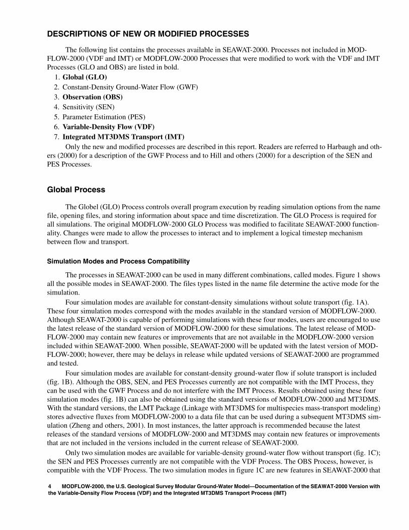
DESCRIPTIONS OF NEW OR MODIFIED PROCESSES

The following list contains the processes available in SEAWAT-2000. Processes not included in MOD-FLOW-2000 (VDF and IMT) or MODFLOW-2000 Processes that were modified to work with the VDF and IMT Processes (GLO and OBS) are listed in bold.

1. Global (GLO)2. Constant-Density Ground-Water Flow (GWF)3. Observation (OBS)4. Sensitivity (SEN)5. Parameter Estimation (PES)6. Variable-Density Flow (VDF)7. Integrated MT3DMS Transport (IMT)

Only the new and modified processes are described in this report. Readers are referred to Harbaugh and oth-ers (2000) for a description of the GWF Process and to Hill and others (2000) for a description of the SEN and PES Processes.

Global Process

The Globel (GLO) Process controls overall program execution by reading simulation options from the name file, opening files, and storing information about space and time discretization. The GLO Process is required for all simulations. The original MODFLOW-2000 GLO Process was modified to facilitate SEAWAT-2000 function-ality. Changes were made to allow the processes to interact and to implement a logical timestep mechanism between flow and transport.

Simulation Modes and Process Compatibility

The processes in SEAWAT-2000 can be used in many different combinations, called modes. Figure 1 shows all the possible modes in SEAWAT-2000. The files types listed in the name file determine the active mode for the simulation.

Four simulation modes are available for constant-density simulations without solute transport (fig. 1A). These four simulation modes correspond with the modes available in the standard version of MODFLOW-2000. Although SEAWAT-2000 is capable of performing simulations with these four modes, users are encouraged to use the latest release of the standard version of MODFLOW-2000 for these simulations. The latest release of MOD-FLOW-2000 may contain new features or improvements that are not available in the MODFLOW-2000 version included within SEAWAT-2000. When possible, SEAWAT-2000 will be updated with the latest version of MOD-FLOW-2000; however, there may be delays in release while updated versions of SEAWAT-2000 are programmed and tested.

Four simulation modes are available for constant-density ground-water flow if solute transport is included (fig. 1B). Although the OBS, SEN, and PES Processes currently are not compatible with the IMT Process, they can be used with the GWF Process and do not interfere with the IMT Process. Results obtained using these four simulation modes (fig. 1B) can also be obtained using the standard versions of MODFLOW-2000 and MT3DMS. With the standard versions, the LMT Package (Linkage with MT3DMS for multispecies mass-transport modeling) stores advective fluxes from MODFLOW-2000 to a data file that can be used during a subsequent MT3DMS sim-ulation (Zheng and others, 2001). In most instances, the latter approach is recommended because the latest releases of the standard versions of MODFLOW-2000 and MT3DMS may contain new features or improvements that are not included in the versions included in the current release of SEAWAT-2000.

Only two simulation modes are available for variable-density ground-water flow without transport (fig. 1C); the SEN and PES Processes currently are not compatible with the VDF Process. The OBS Process, however, is compatible with the VDF Process. The two simulation modes in figure 1C are new features in SEAWAT-2000 that


CO

NS

TAN

T-D

EN

SIT

YG

RO

UN

D-W

AT

ER

FL

OW

VAR

IAB

LE

-DE

NS

ITY

GR

OU

ND

-WA

TE

R F

LO

W

TRANSPORT INCLUDEDTRANSPORT EXCLUDED

UNCOUPLED FLOW

AND

TRANSPORT

COUPLED FLOW

AND

TRANSPORT

GLO + GWF

GLO + GWF (OBS)

GLO + GWF (OBS + SEN)

GLO + GWF (OBS + SEN + PES)

GLO + GWF + IMT

GLO + GWF (OBS) + IMT

GLO + GWF (OBS + SEN) + IMT

GLO + GWF (OBS + SEN + PES) + IMT

GLO + VDF

GLO + VDF (OBS)

GLO + VDF + IMT

GLO + VDF (OBS) + IMT

GLO + VDF + IMT

GLO + VDF (OBS) + IMT

A B

C

D E

EXPLANATION

GLO

GWF

OBS

SEN

PES

IMT

VDF

GLOBAL PROCESS

GROUND-WATER FLOW PROCESS

OBSERVATION PROCESS

SENSITIVITY PROCESS

PARAMETER ESTIMATION PROCESS

INTEGRATED MT3DMS TRANSPORT PROCESS

VARIABLE-DENSITY FLOW PROCESS

Figure 1. Simulation modes available with the SEAWAT-2000 program.

Descriptions of New or Modified Processes 5

were not included in previous versions of SEAWAT. With these two simulation modes, users specify a fluid den-sity array that is held constant during a stress period. The advantage of these two modes is that a variable-density flow simulation can be performed without simulating solute transport. Although these new simulation modes allow for relatively quick simulations without the timestep constraints required for accurate transport solutions, the modes should only be used if one can safely assume that the fluid density will not change in response to the imposed hydrologic stresses. Inaccurate model predictions may result if these modes are used in circumstances where the fluid density may change in response to the imposed hydrologic stresses.

The two simulation modes in figure 1D are similar to those in figure 1C, except the IMT Process has been included to simulate solute transport. In these two simulation modes (fig. 1D), flow and transport are uncoupled, meaning that the flow solution is affected only by the user-specified density array. Thus, the flow field is not affected by the solute concentrations simulated with the IMT Process. These two simulation modes allow the user to simulate, for example, a contaminant plume near a stationary saltwater interface.

The two modes in figure 1E can be used to simulate coupled variable-density flow and solute transport. With these two modes, fluid density (as used in the VDF Process) is calculated by using an equation of state and the simulated solute concentration. The coupled flow and transport mode is the mode represented by previous versions of SEAWAT. For many problems involving coupled flow and transport, users should be aware that computer runtimes may be exceedingly long because timestep lengths are subject to stability criteria, which are necessary for accurate transport solutions.

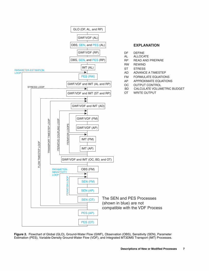
Program Flow

The SEAWAT-2000 program was designed by adding procedure calls to the existing MODFLOW-2000 pro-gram and by adding several new loops. Figure 2, which is a modified version of the flowchart presented by Har-baugh and others (2000), shows the overall structure of the main SEAWAT-2000 program. Although figure 2 has been simplified by grouping some of the procedure calls and by not showing others, the flowchart shows the gen-eral sequence of procedure calls. To some users, SEAWAT-2000 may seem far more complex than the original ver-sion of SEAWAT because of the new processes and functionality included in MODFLOW-2000. This added complexity, however, should be transparent to the experienced user, and in many cases, the SEAWAT-2000 pro-gram will operate similar to, but with more features than, the previous version of SEAWAT.

Numerous loops were added to the MODFLOW-2000 main program to create the VDF and IMT Processes. Three of the new loops most important for illustrating overall program structure are shown in figure 2. The trans-port timestep loop (used for all simulations with solute transport) allows the program to gradually step through each flow timestep using short time increments calculated from the stability criteria. The iterative coupling loop was added for variable-density simulations, allowing the flow and transport equations to be solved repeatedly for the same transport timestep until the solutions converge on fluid density. Lastly, an iteration loop was required for the implicit solver, which is used by the IMT Process to obtain solutions to the solute-transport equation.

Spatial Discretization

The flow processes and the transport process require specific information about the finite-difference grid such as column widths, row heights, and layer tops and bottoms (or layer thicknesses). If the MT3DMS Transport Process is active, then this grid information must be specified as input in two separate files. The current version of SEAWAT-2000 does not verify that the information is consistent. Therefore, users should ensure that grid informa-tion is consistent between the selected flow process and the MT3DMS Transport Process.

Although MODFLOW-2000 requires top and bottom information for each layer, users may still use the quasi-three-dimensional approach to represent semiconfining beds. With SEAWAT-2000, the quasi-three-dimen-sional approach is available; however, users are advised to use the true three-dimensional approach if the MT3DMS Transport Process is active. Use of the quasi-three-dimensional approach can result in inaccurate con-centrations for most solute-transport simulations that include transport through semiconfining layers that are not explicitly represented. Zheng and others (2001) describe a possible exception that is encountered only if solute


GLO (DF, AL, and RP)

GWF/VDF (RP)

GWF/VDF (AL)

OBS, , and (AL)SEN PES

OBS, , and (RP)SEN PES

PES (RW)

GWF and IMT (ST and RP)/VDF

GWF and IMT (AD)/VDF

GWF (FM)/VDF

GWF (AP)/VDF

GWF and IMT (OC, BD, and OT)/VDF

OBS (FM)

SEN (FM)

SEN (AP)

SEN (OT)

PES (AP)

PES (OT)

IMT (AL)

GWF/VDF and IMT (AL and RP)

IMT (FM)

IMT (AP)

PARAMETER-ESTIMATIONLOOP

STRESS LOOP

FLO

WT

IME

ST

EP

LO

OP

TR

AN

SP

OR

TT

IME

ST

EP

LO

OP

PARAMETER-SENSITIVITYLOOP

ITE

RAT

IVE

CO

UP

LIN

G L

OO

P

ITE

RAT

ION

LO

OP

ITE

RAT

ION

LO

OP

S

The SEN and PES Processes(shown in blue) are notcompatible with the VDF Process

DF DEFINEALRPRW

AD

FMAPOCBDOT

ALLOCATEREAD AND PREPAREREWIND

ADVANCE A TIMESTEPFORMULATE EQUATIONSAPPROXIMATE EQUATIONSOUTPUT CONTROLCALCULATE VOLUMETRIC BUDGETWRITE OUTPUT

ST STRESS

EXPLANATION

Figure 2. Flowchart of Global (GLO), Ground-Water Flow (GWF), Observation (OBS), Sensitivity (SEN), Parameter Estimation (PES), Variable-Density Ground-Water Flow (VDF), and Integrated MT3DMS Transport (IMT) Processes.


transport does not occur across the quasi-three-dimensional layer. In this rare circumstance, the MT3DMS Process in SEAWAT-2000 can be used with quasi-three-dimensional semiconfining layers.

Temporal Discretization

The time discretization used in SEAWAT-2000 depends on the active simulation mode. For the simulation modes without solute transport (fig. 1A,C), time discretization follows the standard MODFLOW approach. The simulation is divided into stress periods, and each stress period may be divided into flow timesteps. Users also have an option to allow flow timestep lengths to increase according to a geometric series, which results in shorter flow timesteps at the beginning of the stress period. Results from a simulation, such as heads and flows, can only be saved for times that correspond with the end of a flow timestep. This is also true for variable-density simula-tions with SEAWAT-2000.

For the simulation modes that include solute transport (fig. 1B,D,E), flow timesteps are further divided into transport timesteps. Lengths of transport timesteps are calculated according to stability criteria, or specified by the user if the implicit finite-difference method is used to solve the transport equation (Zheng and Wang, 1999). In SEAWAT-2000, which is primarily designed for simulating variable-density ground-water flow problems, the flow and transport equations are both solved for each transport timestep. This is the approach used in previous versions of SEAWAT. Solutions to both flow and transport are required for each transport timestep because changes in sol-ute concentration can affect flow patterns. In a constant-density system, however, flow timesteps may be much longer than transport timesteps because ground-water flow patterns are unaffected by solute concentrations. This is a limitation of SEAWAT-2000: both flow and transport are solved for each transport timestep, even for con-stant-density systems.

When the standard version of MT3DMS is run separately from the standard version of MODFLOW-2000, the flow solution for the entire simulation period is calculated prior to simulating transport. At the beginning of the MT3DMS simulation, the length of the first transport timestep can be calculated from the stability criteria using the advective velocities from the MODFLOW-2000 simulation. At the beginning of a flow and transport simula-tion with SEAWAT-2000, the length of the first transport timestep cannot be calculated using the stability criteria because the advective velocities are not yet available. Thus, in SEAWAT-2000, the length of the first transport timestep is, by default, set to a value of 0.01 time units. However, users also have the option to specify the length of the first transport timestep in the input file for the VDF Process.

Coupling of Flow and Transport

For variable-density simulations involving coupled flow and transport, SEAWAT-2000 contains explicit and implicit options for solving the flow and transport equations. Guo and Langevin (2002) describe both of these options in detail. The explicit coupling option, also referred to as a “one timestep lag,” is the default option. With the explicit approach, the flow equation is formulated using fluid densities from the previous transport timestep. This approach is conceptually straightforward and is adequate for most variable-density simulations. For simula-tions with rapidly changing solute concentrations, the implicit coupling option may provide a more accurate solu-tion than the explicit option. With the implicit option, the flow and transport equations are solved repeatedly for each transport timestep until consecutive differences in the calculated fluid densities are less than a user-specified value. The implicit coupling option in SEAWAT-2000 can only be used when a MT3DMS finite-difference method (as opposed to a particle-based method) is used to solve the solute-transport equation.

Variable-Density Flow Process

The VDF Process is defined as those parts of SEAWAT-2000 that are used to solve the variable-density ground-water flow equation. This process includes only the variable-density flow equation and does not include the solute-transport equation. To perform a coupled, variable-density, ground-water flow and solute-transport sim-ulation, the IMT Process must also be active.


The VDF Process was developed by modifying the GWF Process of MODFLOW-2000 to solve a variable-density form of the ground-water flow equation. Necessary modifications include: (1) addition of relative density-difference terms, (2) addition of solute mass accumulation terms, (3) conservation of mass rather than volume, (4) use of head instead of equivalent freshwater head in conversions between confined and unconfined conditions, (5) addition of variable-density correction terms for dewatered conditions, and (6) addition of variable-density cor-rection terms for the water-table case. Guo and Langevin (2002) present the derivations and detailed descriptions for each of these required modifications.

Use of Head and Equivalent Freshwater Head in SEAWAT-2000

The VDF Process in SEAWAT-2000 uses equivalent freshwater head as the dependent variable in the variable-density ground-water flow equation. By using equivalent freshwater head rather than pressure, the MODFLOW structure and subroutines can be used with few modifications to solve the variable-density ground-water flow equation.

The concept of equivalent freshwater head is best explained by using water levels measured in a well. Con-sider a monitoring well with a short screened opening in a saline aquifer. The water level in the well is a measure of head, h, in terms of aquifer water. If the saline water within the well were replaced with freshwater, the water level in the well would be higher because more freshwater would be required to equal the weight of the saline aquifer water. The new water level in the well would be a measure of head in terms of freshwater, called the equiv-alent freshwater head, hf.

Conversions between h and hf can be made using the following equations (Guo and Langevin, 2002):

(1)

and

, (2)

where ρ is the density of the native aquifer water [ML-3]; ρf is the density of freshwater [ML-3]; and Z is the elevation at the measurement point [L].

With the previous version of SEAWAT, input and output were expressed in terms of equivalent freshwater head. In most cases, this required additional effort by the modeler to convert between head and equivalent freshwa-ter head before and after simulations. In SEAWAT-2000, input and output are expressed in terms of the head of the native aquifer water. SEAWAT-2000 converts the input head values using equation 1 into equivalent freshwater head using densities calculated from the initial concentrations. After a solution to the variable-density ground-water flow equation is obtained (in terms of equivalent freshwater head), the program uses equation 2 to convert to head using the calculated density. Head data written to the output files, therefore, are expressed in terms of the density of the aquifer water. Users can then use the output head data to directly compare with water levels mea-sured in wells and prepare contour maps of the water table or potentiometric surface.

Variable-Density Ground-Water Flow Equation

Guo and Langevin (2002) derive the governing equation for variable-density ground-water flow, in terms of equivalent freshwater head, as:

hfρρf----h

ρ ρf–

ρf-----------Z–=

hρfρ----hf

ρ ρf–

ρ--------------Z+=


, (3)

where α, β, γ are orthogonal coordinate axes, aligned with the principal directions of permeability; Kf is equiva-lent freshwater hydraulic conductivity [LT-1]; Sf is equivalent freshwater specific storage [L-1]; t is time [T]; θ is effective porosity [dimensionless]; C is solute concentration [ML-3]; ρs is fluid density source or sink water [ML-

3]; and qs is the volumetric flow rate of sources and sinks per unit volume of aquifer [T-1]. The VDF Process in SEAWAT-2000 has two different options for treating the density terms in equation 3.

With the simplest option, and the one that would result in the fastest computer runtimes, the user specifies a fluid density array (or a concentration array that is converted by the program to fluid density using the equation of state) that is held constant during a stress period or simulation. The other option is to calculate fluid densities using the equation of state and solute concentrations from the IMT Process. With this type of simulation, flow and transport are coupled, and thus, the lengths of timesteps may be subject to stability criteria.

For a coupled variable-density flow and solute-transport simulation, fluid density is assumed to be a func-tion only of solute concentration; the effects of pressure and temperature on fluid density are not considered. A lin-ear equation of state is used to represent fluid density as a function of solute concentration:

. (4)

Values for ρf and ∂ρ/∂C are entered by the user and depend on the units used for the simulation. For most simulations, ρf is set to the density of freshwater, and ∂ρ/∂C is calculated for the range of expected densities and concentrations. For example, if meters and kilograms are used for the simulation, ∂ρ/∂C is set to a value of 0.7143, which approximately equals the change in fluid density divided by the change in solute concentration for freshwa-ter and seawater. The value of 0.7143 may not be appropriate for all cases if the end-member fluids are not fresh-water and typical seawater. In these circumstances, a unique relation between density and concentration may be developed using field data. Users also have the option to specify a reference fluid density, ρf, other than the density of freshwater. The reference fluid density corresponds to the density of a fluid with zero concentration.

A new feature in SEAWAT-2000 is the option for the user to enter minimum and maximum density values, referred to here as density limiters. In some instances, numerical problems will cause the IMT Process to result in unrealistic and erroneous concentrations. For example, some of the transport solvers in MT3DMS can result in negative concentrations. If a negative concentration is used in the equation of state, a density value less than fresh-water will be calculated. For example, the minimum density limiter can be used to limit densities to only those val-ues greater than the density of freshwater. The maximum density limiter can be used to reduce the impact of unreasonably high concentrations on the flow equation.

Another new feature in SEAWAT-2000 is the capability to select which MT3DMS species is used in the equation of state. For most simulations, this number will be the MT3DMS species number corresponding to total dissolved solids or chloride concentration. In the previous version of SEAWAT, the first MT3DMS species was always used in the equation of state, and constantly had to represent total dissolved solids. With the new feature, users can specify the concentration of the third species, for example, to use in the equation of state. If the user specifies zero for the MT3DMS species, then fluid densities are entered in the input file for the VDF Process.

The VDF Process solves equation 3 using a cell-centered finite-difference approximation, written as (Guo and Langevin, 2002):

∂∂α------- ρKfα

∂hf∂α-------

ρ ρf–

ρf-------------- ∂Z

∂α-------+⎝ ⎠

⎛ ⎞ ∂∂β------ ρKfβ

∂hf∂β-------

ρ ρf–

ρf-------------- ∂Z

∂β------+⎝ ⎠

⎛ ⎞+

∂∂γ----- ρKfγ

∂hf∂γ-------

ρ ρf–

ρf-------------- ∂Z

∂γ------+⎝ ⎠

⎛ ⎞+ ρSf∂hf∂t------- θ ∂ρ

∂C------- ∂C

∂t------- ρsqs–+=

ρ ρf∂ρ∂C-------C+=


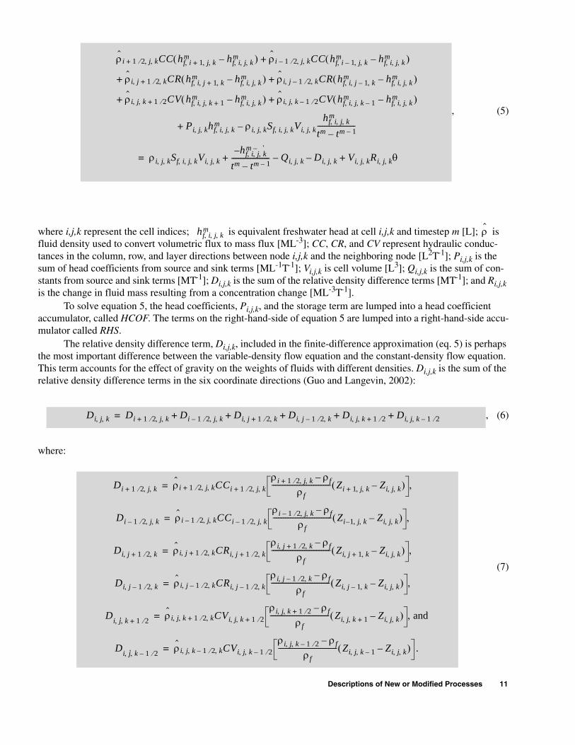
, (5)

where i,j,k represent the cell indices; is equivalent freshwater head at cell i,j,k and timestep m [L]; is fluid density used to convert volumetric flux to mass flux [ML-3]; CC, CR, and CV represent hydraulic conduc-tances in the column, row, and layer directions between node i,j,k and the neighboring node [L2T-1]; Pi,j,k is the sum of head coefficients from source and sink terms [ML-1T-1]; Vi,j,k is cell volume [L3]; Qi,j,k is the sum of con-stants from source and sink terms [MT-1]; Di,j,k is the sum of the relative density difference terms [MT-1]; and Ri,j,k is the change in fluid mass resulting from a concentration change [ML-3T-1].

To solve equation 5, the head coefficients, Pi,j,k, and the storage term are lumped into a head coefficient accumulator, called HCOF. The terms on the right-hand-side of equation 5 are lumped into a right-hand-side accu-mulator called RHS.

The relative density difference term, Di,j,k, included in the finite-difference approximation (eq. 5) is perhaps the most important difference between the variable-density flow equation and the constant-density flow equation. This term accounts for the effect of gravity on the weights of fluids with different densities. Di,j,k is the sum of the relative density difference terms in the six coordinate directions (Guo and Langevin, 2002):

, (6)

where:

(7)

ρ̂i 1 2 j k, ,⁄+ CC hf i 1 j k, ,+,m hf i j k, , ,

m–( ) ρ̂i 1 2 j k, ,⁄– CC hf i 1 j k, ,–,m hf i j k, , ,

m–( )+

ρ̂i j 1 2 k,⁄+,+ CR hf i j, 1 k,+,m hf i j k, , ,

m–( ) ρ̂i j, 1 2 k,⁄– CR hf i j, 1 k,–,m hf i j k, , ,

m–( )+

ρ̂+ i j k, , 1 2⁄+ CV hf i j k, , 1+,m hf i j k, , ,

m–( ) ρ̂i j k, , 1 2⁄– CV hf i j k, , 1–,m hf i j k, , ,

m–( )+

Pi j k, , hf i j k, , ,m ρi j k, , Sf i j k, , , Vi j k, ,

hf i j k, , ,m

tm tm 1––----------------------–+

ρi j k, , Sf i j k, , , Vi j k, ,hf i j k, , ,

m '––

tm tm 1––---------------------- Qi j k, ,– Di j k, ,– Vi j k, , Ri j k, , θ+ +=

hf i j k, , ,m ρ̂

Di j k, , Di 1 2 j k, ,⁄+ Di 1 2 j k, ,⁄– Di j 1 2 k,⁄+, Di j 1 2 k,⁄–, Di j k 1 2⁄+, , Di j k, 1 2⁄–,+ + + + +=

Di 1 2 j k, ,⁄+ ρ̂i 1 2 j k, ,⁄+ CCi 1 2 j k, ,⁄+

ρi 1 2 j k, ,⁄+ ρf–

ρf---------------------------------- Zi 1 j k, ,+ Zi j k, ,–( ) ,=

Di 1 2 j k, ,⁄– ρ̂i 1 2 j k, ,⁄– CCi 1 2 j k, ,⁄–

ρi 1 2 j k, ,⁄– ρf–

ρf---------------------------------- Zi 1– j k, , Zi j k, ,–( ) ,=

Di j, 1 2 k,⁄+ ρ̂i j, 1 2 k,⁄+ CRi j, 1 2 k,⁄+

ρi j, 1 2 k,⁄+ ρf–

ρf---------------------------------- Zi j, 1 k,+ Zi j k, ,–( ) ,=

Di j, 1 2 k,⁄– ρ̂i j, 1 2 k,⁄– CRi j, 1 2 k,⁄–

ρi j, 1 2 k,⁄– ρf–

ρf---------------------------------- Zi j, 1 k,– Zi j k, ,–( ) ,=

Di j· k, , 1 2⁄+ρ̂i j k, , 1 2 k,⁄+ CVi j k, , 1 2⁄+

ρi j k, , 1 2⁄+ ρf–

ρf---------------------------------- Zi j k, , 1+ Zi j k, ,–( ) and,=

Di j· k, , 1 2⁄–ρ̂i j k, , 1 2 k,⁄– CVi j k, , 1 2⁄–

ρi j k, , 1 2⁄– ρf–

ρf---------------------------------- Zi j k, , 1– Zi j k, ,–( ) .=


Equations 5 and 7 contain two different types of density terms; namely, ρ and . The first type, ρ, is used to calculate the weight of the fluid and is evaluated using a simple central-in-space algorithm in which densities are weighted based on adjacent cell lengths. For example, the density at the point between cell i,j,k and i,j,k+1 is cal-culated with the following equation:

(8)

The second type of density term, , is used to conserve mass by converting volumetric flux to mass flux.

The VDF Process contains two options for calculating . The first option uses the same central-in-space weight-ing algorithm used to calculate ρ. The second option uses an upstream weighting algorithm in which the density value is selected based on the flow direction during that particular iteration. Results from variable-density simula-

tions do not appear to be sensitive to the option used to calculate ; however users may want to experiment with both options.

The Ri,j,k term is used to account for the change in fluid mass that results from a change in solute concentra-tion. Depending on the coupling method for the flow and transport equations (the user can select either explicit or implicit), this term is evaluated using concentrations from the two previous transport timesteps (explicit):

, (9)

or is evaluated using concentrations from a previous coupling iteration (implicit):

, (10)

where ρ(C) is the fluid density as a function of solute concentration calculated using the equation of state (eq. 4) [ML-3]; and m* is a previous coupling iteration of timestep m.

During iterations of the variable-density flow equation, the HCOF and RHS accumulators are assembled, and a solver package approximates the solution for equivalent freshwater head. This sequence repeats until the solution for equivalent freshwater head meets the user-specified error tolerances.

Required and Optional Flow-Related Packages Included in this Report

Numerous packages have been developed for the suite of MODFLOW programs. This section briefly describes the packages that are required for a variable-density flow simulation and also the flow-related packages that are compatible with the VDF Process. A list of all the packages that can be used for a variable-density simula-tion is given in table 1.

ρ̂

ρi j k, 1 2⁄+,ρi j k, , Zi j k, , Zi j k 1 2⁄+, ,–( ) ρi j k 1+, , Zi j k 1 2⁄+, , Zi j k 1+, ,–( )+

Zi j k, , Zi j k 1+, ,–--------------------------------------------------------------------------------------------------------------------------------------------=

ρ̂

ρ̂

ρ̂

Ri j k, ,ρ Ci j k, ,

m 1–( ) ρ Ci j k, ,m 2–( )–

tm 1– tm 2––---------------------------------------------------=

Ri j k, ,ρ Ci j k, ,

m∗( ) ρ Ci j k, ,m 1–( )–

tm tm 1––--------------------------------------------------=


Basic (BAS6) Package

The VDF Process requires the use of the MODFLOW-2000 Basic (BAS6) Package to specify active, inac-tive, or constant-head cells and to assign initial heads. With a standard MODFLOW-2000 simulation, the BAS6 Package is often used to specify constant-head cells by specifying appropriate values for the boundary array and the initial heads. If constant-head cells are specified using this method, rather than using the Time-Variant Con-stant-Head (CHD) Package, the initial heads are converted to equivalent freshwater heads using the initial densi-ties. This equivalent freshwater head value is then used for the rest of the simulation.

Table 1. List of packages and files that can be used for a variable-density flow and solute-transport simulation

[Source: 1, Harbaugh and others (2000); 2, McDonald and Harbaugh (1988); 3, Anderman and Hill (2000); 4, Hsieh and Freckleton (1993); 5, Leake and Prudic (1991); 6, Hill (1990); 7, Harbaugh (1995); 8, Mehl and Hill (2001); 9, Zheng and others (2001); 10, Zheng and Wang (1999); 11, Hill and others (2000)]

Process Package or file name File type Source

GLO

Global GLOBAL 1List LIST 1Discretization DIS 1Multiplier MULT 1Zone ZONE 1

VDF

Variable-Density Flow VDFBasic BAS6 1,2Block-Centered Flow BCF6 1,2Layer-Property Flow LPF 1Hydrogeologic-Unit Flow HUF 3Hydraulic Flow Barrier HFB6 1,4Drain DRN 1,2River RIV 1,2General-Head Boundary GHB 1,2Evapotranspiration EVT 1,2Well WEL 1,2Recharge RCH 1,2Time-Variant Constant Head CHD 1,5Strongly Implicit Procedure SIP 1,2Slice-Successive Overrelaxation SOR 1,2Preconditioned Conjugate Gradient PCG 1,6Direct Solver DE4 1,7Link-Algebraic Multi-Grid LMG 8Linkage with MT3DMS LMT6 9

IMT

Basic Transport BTN 10Advection ADV 10Dispersion DSP 10Source-Sink Mixing SSM 10Chemical Reaction RCT 10Generalized Conjugate Gradient GCG 10

OBS

Observation OBS 11Hydraulic-Head Observation HOB 11General-Head Boundary Observation GHOB 11Drain Observation DROB 11River Observation RVOB 11Constant-Head Flow Observation CHOB 11


Internodal Conductance Packages

The VDF Process requires that one of the three conductance packages is active during a simulation to calcu-late the internodal conductance arrays and update conductances during iterations of the variable-density flow equation. Users must select one package from the following three choices:• Block Centered Flow - BCF6 (Harbaugh and others, 2000),• Layer-Property Flow - LPF (Harbaugh and others, 2000), or• Hydrogeologic-Unit Flow - HUF (Anderman and Hill, 2000).

The BCF6 Package in MODFLOW-2000 is similar to the BCF package in previous versions of MODFLOW, except that the input file for the BCF6 package does not contain the steady-state flag or discretization information. Therefore, SEAWAT-2000 cannot read BCF packages created for previous versions of SEAWAT. The internal equations of the BCF6 Package were modified to work with the VDF Process much like the BCF Package was modified to work with earlier versions of SEAWAT (Guo and Langevin, 2002). For example, internodal fluxes are represented in terms of mass rather than volume, and variable-density corrections are required for the water-table case, confined/unconfined conversions, and vertical flow between partially saturated cells.

The LPF Package is an alternative to the BCF6 Package for calculating internodal conductance values in MODFLOW-2000 or SEAWAT-2000. The LPF Package is similar to the BCF6 Package, with the exception of input requirements. The LPF Package in SEAWAT-2000 was modified to work with the VDF Process in a similar way as the BCF6 Package.

The HUF Package is another alternative to the BCF6 Package in MODFLOW-2000 and SEAWAT-2000. The HUF Package allows users to enter sloping or irregular hydrogeologic units. These units are then intersected with the model grid, and the program calculates the internodal conductance values.

The HFB6 Package (Hsieh and Freckleton, 1993; Harbaugh and others, 2000) can be used to simulate hori-zontal flow barriers by modifying internodal conductance values based on barrier properties. The HFB6 Package is compatible with the three other conductance packages described above. There are no restrictions on the usage of this package while running a flow simulation; however, the IMT Process may calculate inaccurate dispersive fluxes near horizontal flow barriers (Hornberger and others, 2002).

Source-Term Packages

The following six source-term packages are compatible with the VDF Process:• Drain (DRN),• River (RIV), • General-Head Boundary (GHB),• Evapotranspiration (EVT),• Well (WEL), and• Recharge (RCH).McDonald and Harbaugh (1988) originally described these packages, and Harbaugh and others (2000) describe their implementation in MODFLOW-2000. Guo and Langevin (2002) describe how these packages are modified to function for variable-density conditions within SEAWAT. A similar approach is used to allow these packages to function with SEAWAT-2000.

The DRN, RIV, GHB, and EVT Packages are head dependent because the flow rate to or from the boundary is dependent on the head value within the adjacent model cell. The WEL and RCH Packages are considered head-independent packages because the user specifies the flow rate to or from the boundary.

Time-Variant Constant-Head (CHD) Package

The Time-Variant Constant-Head (CHD) Package (Leake and Prudic, 1991; Harbaugh and others, 2000) is compatible with the VDF Process. This package allows the head value assigned to constant-head boundaries to vary within a stress period and between stress periods. With the CHD Package, the user enters a starting and end-ing head value for each stress period. The program then interpolates a head value for each flow or transport


timestep based on the time elapsed in the stress period. This head value is then converted to an equivalent freshwa-ter head using the density value for that transport timestep.

Solver Packages

The VDF Process assembles the matrix equations in a form that is identical to that used by the Constant-Density Ground-Water Flow (GWF) Process. By using the same form of the matrix equations, the VDF Process can use the solvers that have been designed for the GWF Process without any modifications. Therefore, the fol-lowing solver packages included with MODFLOW-2000 can be used directly with the VDF Process:• Strongly Implicit Procedure (SIP),• Slice-Successive Overrelaxation (SOR),• Preconditioned Conjugate Gradient (PCG),• Direct Solver (DE4), and• Link-Algebraic Multi-Grid (LMG).

Although modifications were not required for the solvers to work with the VDF Process, there is a differ-ence in the data that is passed into the active solver. With the GWF Process, internodal conductance values are passed directly into the active solver. With the VDF Process, however, mass is conserved instead of volume, and thus, the internodal conductance values passed into the active solver have been multiplied by fluid density (Guo and Langevin, 2002).

Link-MT3DMS (LMT6) Package

The Link-MT3DMS (LMT6) package is currently used two different ways in the SEAWAT-2000 program. The first use, which is transparent to the user, is to pass saturated thicknesses and advective fluxes from the VDF or GWF Processes into the IMT Process. The other use is to allow the GWF or VDF Processes to store advective fluxes to a computer file that can be used for subsequent transport simulations with the standard version of MT3DMS.

Integrated MT3DMS Transport (IMT) Process

The MT3DMS computer program (Zheng and Wang, 1999), which normally runs as a separate program from MODFLOW, was integrated directly into SEAWAT-2000. This new capability is called the Integrated MT3DMS Transport (IMT) Process. The main purpose for integrating MT3DMS directly into SEAWAT-2000 is for variable-density simulations where flow and transport are coupled processes, and thus, the flow and transport equations must be solved sequentially (explicit) or simultaneously (implicit) for each timestep. This requirement eliminates the possibility for maintaining MT3DMS and SEAWAT-2000 as separate programs. Although the IMT Process was added primarily to work with the VDF Process, this new process also has been designed to work with the GWF Process. This option provides users with the ability to perform constant-density (and variable-density) flow and transport simulations with a single program. As stated in the “Temporal Discretization” section, however, the flow equation is solved for every transport timestep rather than for every flow timestep. This means that con-stant-density simulations of flow and transport with SEAWAT-2000 may take longer than simulations with stan-dard versions of MODFLOW-2000 and MT3DMS. The results, however, should be similar.

The IMT Process was created for SEAWAT-2000 by adding the subroutines from the MT3DMS program directly to MODFLOW-2000. Fortunately, the MT3DMS source code required few modifications to integrate the program directly into SEAWAT-2000. New versions of MT3DMS, therefore, should be relatively easy to incorpo-rate into SEAWAT-2000, provided the overall structures of the two programs do not change.

The IMT Process simulates advective and dispersive transport and simple chemical reactions for multiple species. In SEAWAT-2000, the concentrations from only one of these species are used in the equation of state to calculate fluid density.


Solute-Transport Equations

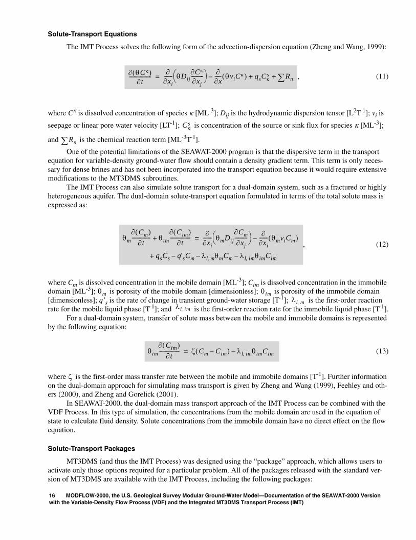
The IMT Process solves the following form of the advection-dispersion equation (Zheng and Wang, 1999):

, (11)

where Cκ is dissolved concentration of species κ [ML-3]; Dij is the hydrodynamic dispersion tensor [L2T-1]; vi is

seepage or linear pore water velocity [LT-1]; is concentration of the source or sink flux for species κ [ML-3];

and is the chemical reaction term [ML-3T-1].

One of the potential limitations of the SEAWAT-2000 program is that the dispersive term in the transport equation for variable-density ground-water flow should contain a density gradient term. This term is only neces-sary for dense brines and has not been incorporated into the transport equation because it would require extensive modifications to the MT3DMS subroutines.

The IMT Process can also simulate solute transport for a dual-domain system, such as a fractured or highly heterogeneous aquifer. The dual-domain solute-transport equation formulated in terms of the total solute mass is expressed as:

, (12)

where Cm is dissolved concentration in the mobile domain [ML-3]; Cim is dissolved concentration in the immobile domain [ML-3]; is porosity of the mobile domain [dimensionless]; is porosity of the immobile domain [dimensionless]; q’s is the rate of change in transient ground-water storage [T-1]; is the first-order reaction rate for the mobile liquid phase [T-1]; and is the first-order reaction rate for the immobile liquid phase [T-1].

For a dual-domain system, transfer of solute mass between the mobile and immobile domains is represented by the following equation:

(13)

where is the first-order mass transfer rate between the mobile and immobile domains [T-1]. Further information on the dual-domain approach for simulating mass transport is given by Zheng and Wang (1999), Feehley and oth-ers (2000), and Zheng and Gorelick (2001).

In SEAWAT-2000, the dual-domain mass transport approach of the IMT Process can be combined with the VDF Process. In this type of simulation, the concentrations from the mobile domain are used in the equation of state to calculate fluid density. Solute concentrations from the immobile domain have no direct effect on the flow equation.

Solute-Transport Packages

MT3DMS (and thus the IMT Process) was designed using the “package” approach, which allows users to activate only those options required for a particular problem. All of the packages released with the standard ver-sion of MT3DMS are available with the IMT Process, including the following packages:

∂ θCκ( )∂t

------------------∂

∂xi------- θDij

∂Cκ

∂xj----------⎝ ⎠

⎛ ⎞ ∂∂x----- θviCκ( )– qsCκ

s Rn∑++=

Cκs

Rn∑

θm∂ Cm( )

∂t--------------- θim

∂ Cim( )∂t

-----------------+∂

∂xi------- θmDij

∂Cm∂xj

----------⎝ ⎠⎛ ⎞ ∂

∂xi------- θmviCm( )–=

qsCs q'sCm– λl m, θmCm– λl im, θimCim–+

θm θimλl m,

λl im,

θim∂ Cim( )

∂t----------------- ζ Cm Cim–( ) λl im, θimCim–=

ζ


• Basic Transport (BTN);• Advection (ADV);• Dispersion (DSP);• Source-Sink Mixing (SSM);• Chemical Reaction (RCT); and• Generalized Conjugate Gradient (GCG).

Observation (OBS) Process

The Observation (OBS) Process calculates simulated equivalents for observed (measured) flow-related data, such as heads and boundary flows. The OBS Process compares simulated equivalents with the observation data and calculates observation sensitivities if the Sensitivity (SEN) Process is active. The OBS Process, which is included with the standard version of MODFLOW-2000, was modified to work with the VDF Process; however, the OBS Process has not yet been programmed to work with solute concentrations. Therefore, because the VDF and SEN processes are incompatible, observation sensitivities cannot be calculated for the VDF Process. A vari-able-density form of Darcy’s Law was implemented to calculate head-dependent flows to or from a boundary. Modifications were required for the OBS Process to accurately calculate flows for the GHB, DRN, and RIV Pack-ages and for constant-head cells. These modifications are transparent to the user, and the OBS Process will work for constant-density or variable-density simulations in the manner described by Hill and others (2000).

INPUT INSTRUCTIONS

Most of the input files required by SEAWAT-2000 are described in the original documentations for those processes. For example, input instructions for the GWF Process are described in Harbaugh and others (2000), and because the VDF Process was created from the GWF Process, most of those input instructions are also listed in Harbaugh and others (2000). This section describes only input instructions or special considerations specific to SEAWAT-2000. Users are referred to the original documentations for more detailed instructions.

Global (GLO) Process Input Instructions

The name, discretization, multiplier, and zone files are all input for the Global (GLO) Process. The name and discretization files both contain special requirements for SEAWAT-2000 and are described in the following sections. There are no special requirements for the multiplier and zone files.

Name (NAM) File

When the SEAWAT-2000 program is executed, a name file is requested. The file types listed in the name (NAM) file control which processes and packages are active for the simulation. The NAM file is read on unit 99 and is constructed as follows:

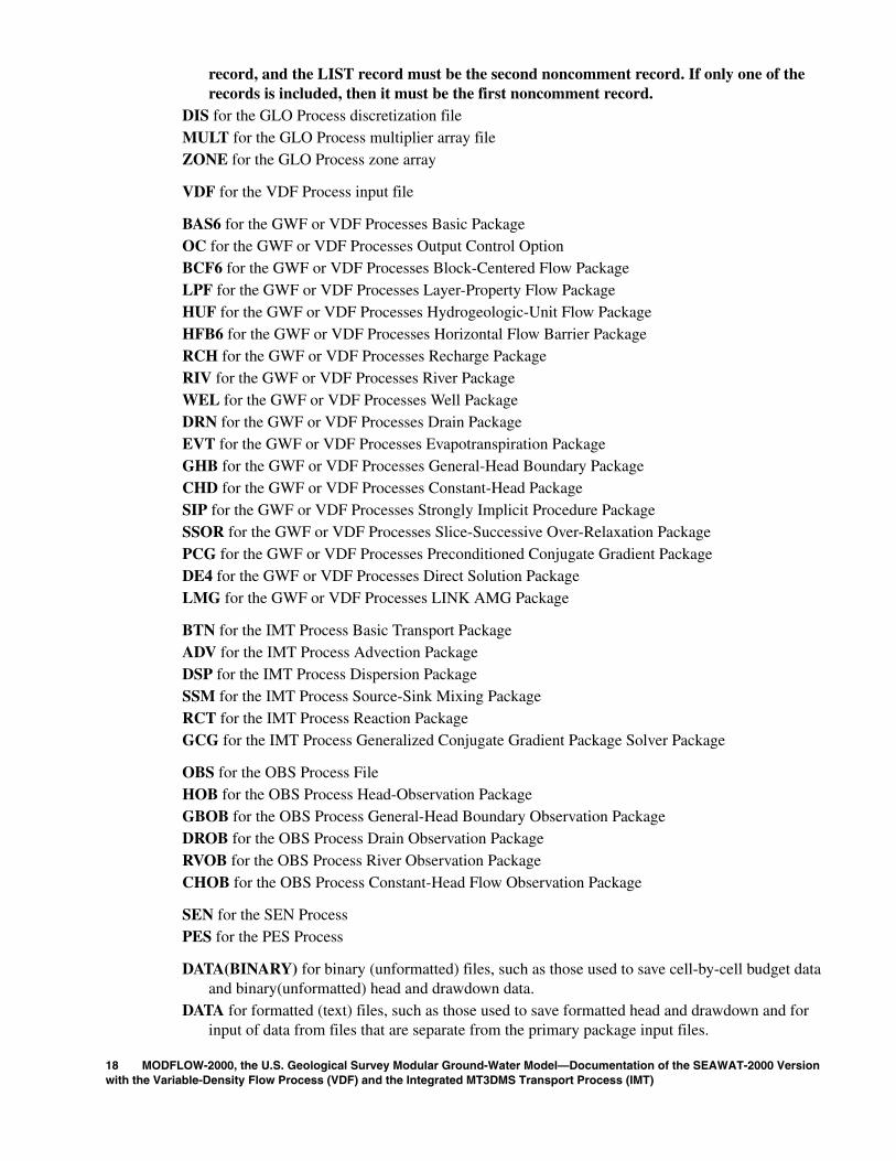
FOR EACH SIMULATIONItem 1. FTYPE Nunit FnameFTYPE—is the file type, which must be one of the following character values. FTYPE may be entered in all uppercase, all lowercase, or any combination. Potential character values for FTYPE are listed here in bold to show the processes and packages available in SEAWAT-2000.

GLOBAL for the global listing file—If this type is not present, then the LIST file is used for the global listing file as well as for the forward run listing file.

LIST for the forward run listing file—if this type is not present, then the GLOBAL file is used for the forward run listing as well as for the global run listing file.The NAM file must always include a record that specifies GLOBAL or LIST for FTYPE. Both records can be included, and if so, the GLOBAL record must be the first noncomment

Input Instructions 17

record, and the LIST record must be the second noncomment record. If only one of the records is included, then it must be the first noncomment record.

DIS for the GLO Process discretization fileMULT for the GLO Process multiplier array fileZONE for the GLO Process zone array

VDF for the VDF Process input file

BAS6 for the GWF or VDF Processes Basic PackageOC for the GWF or VDF Processes Output Control OptionBCF6 for the GWF or VDF Processes Block-Centered Flow PackageLPF for the GWF or VDF Processes Layer-Property Flow PackageHUF for the GWF or VDF Processes Hydrogeologic-Unit Flow PackageHFB6 for the GWF or VDF Processes Horizontal Flow Barrier PackageRCH for the GWF or VDF Processes Recharge PackageRIV for the GWF or VDF Processes River PackageWEL for the GWF or VDF Processes Well PackageDRN for the GWF or VDF Processes Drain PackageEVT for the GWF or VDF Processes Evapotranspiration PackageGHB for the GWF or VDF Processes General-Head Boundary PackageCHD for the GWF or VDF Processes Constant-Head PackageSIP for the GWF or VDF Processes Strongly Implicit Procedure PackageSSOR for the GWF or VDF Processes Slice-Successive Over-Relaxation PackagePCG for the GWF or VDF Processes Preconditioned Conjugate Gradient PackageDE4 for the GWF or VDF Processes Direct Solution PackageLMG for the GWF or VDF Processes LINK AMG Package

BTN for the IMT Process Basic Transport PackageADV for the IMT Process Advection PackageDSP for the IMT Process Dispersion PackageSSM for the IMT Process Source-Sink Mixing PackageRCT for the IMT Process Reaction PackageGCG for the IMT Process Generalized Conjugate Gradient Package Solver Package

OBS for the OBS Process FileHOB for the OBS Process Head-Observation PackageGBOB for the OBS Process General-Head Boundary Observation PackageDROB for the OBS Process Drain Observation PackageRVOB for the OBS Process River Observation PackageCHOB for the OBS Process Constant-Head Flow Observation Package

SEN for the SEN Process PES for the PES Process

DATA(BINARY) for binary (unformatted) files, such as those used to save cell-by-cell budget data and binary(unformatted) head and drawdown data.

DATA for formatted (text) files, such as those used to save formatted head and drawdown and for input of data from files that are separate from the primary package input files.


Discretization (DIS) File

Discretization information is read from the file that is specified by “DIS” as the file type. When the VDF and IMT Processes are run together in coupled mode, an additional level of vertical discretization may be required compared to a similar constant-density simulation. Special considerations for some variables in the DIS file are described here.

Item 2. LAYCBD(NLAY)

LAYCBD—is a flag, with one value for each model layer that indicates whether a layer is underlain by a quasi-three-dimensional confining bed. Zero indicates no confining bed, and numbers other than zero indicate a confin-ing bed. LAYCBD for the bottom layer must be zero. Quasi-three-dimensional confining beds should be used only in special cases where the IMT Process is active. One special case is when solute does not move through the quasi-three-dimensional confining bed.

Item 7. PERLEN NSTP TSMULT SS/TR

SS/TR—is a character variable that indicates whether the stress period is transient or steady state. The only allowed options are “SS” and “TR,” but these are case insensitive. If the IMT Process is activated, and “SS” is specified for a stress period, then the VDF or GWF Process will solve a steady-state form of the flow equation. This does not mean the IMT Process will calculate steady-state solute concentrations in a single transport timestep. Steady-state solute concentrations can only be obtained by gradually stepping through time until concen-trations no longer change.

Variable-Density Flow (VDF) Process Input Instructions

Input instructions for the Variable-Density Flow (VDF) Process are similar to the input instructions for the GWF Process. Differences between the two and special considerations for the VDF Process are described in the following sections. Also described is a specific input file required by the VDF Process. The VDF Process is acti-vated by including VDF as a file type in the name file; otherwise, the simulation uses the GWF Process.

Variable-Density Flow (VDF) Process Input File

Input for the Variable-Density Flow (VDF) Process is read from the file that is specified with “VDF” as the file type. This is a new file type introduced with SEAWAT-2000. All single-valued variables are free format if the option “FREE” is specified in the Basic Package input file; otherwise, the variables have 10-character fields.FOR EACH SIMULATION0. [#Text]

Item 0 is optional and the symbol # must be in column 1. Item 0 can be repeated multiple times.1. MTDNCONC MFNADVFD NSWTCPL IWTABLE

2. DENSEMIN DENSEMAX

If NSWTCPL is greater than 1, then read item 3.3. DNSCRIT

4. DENSEREF DENSESLP

5. FIRSTDT

FOR EACH STRESS PERIOD (read items 6 and 7 only if MTDNCONC = 0)6. INDENSE

Read item 7 only if INDENSE is greater than zero7. [DENSE(NCOL,NROW)] – U2DREL

Item 7 is read for each layer in the grid.


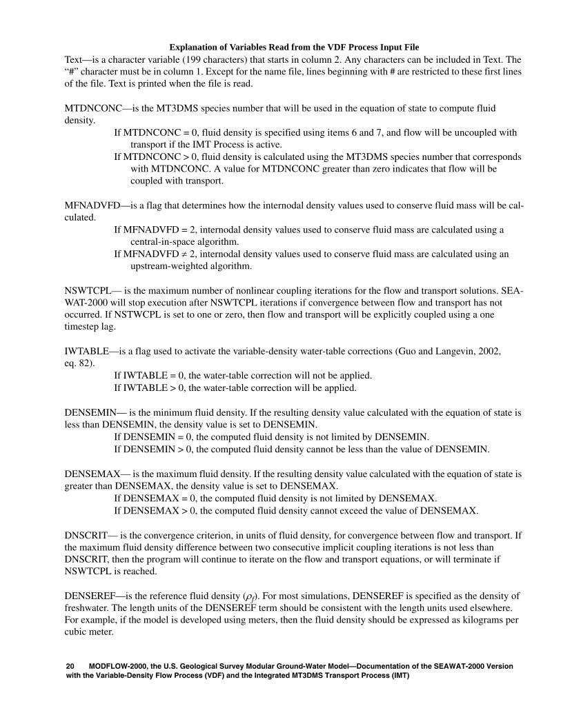
Explanation of Variables Read from the VDF Process Input FileText—is a character variable (199 characters) that starts in column 2. Any characters can be included in Text. The “#” character must be in column 1. Except for the name file, lines beginning with # are restricted to these first lines of the file. Text is printed when the file is read.

MTDNCONC—is the MT3DMS species number that will be used in the equation of state to compute fluid density.

If MTDNCONC = 0, fluid density is specified using items 6 and 7, and flow will be uncoupled with transport if the IMT Process is active.

If MTDNCONC > 0, fluid density is calculated using the MT3DMS species number that corresponds with MTDNCONC. A value for MTDNCONC greater than zero indicates that flow will be coupled with transport.

MFNADVFD—is a flag that determines how the internodal density values used to conserve fluid mass will be cal-culated.

If MFNADVFD = 2, internodal density values used to conserve fluid mass are calculated using a central-in-space algorithm.

If MFNADVFD ≠ 2, internodal density values used to conserve fluid mass are calculated using an upstream-weighted algorithm.

NSWTCPL— is the maximum number of nonlinear coupling iterations for the flow and transport solutions. SEA-WAT-2000 will stop execution after NSWTCPL iterations if convergence between flow and transport has not occurred. If NSTWCPL is set to one or zero, then flow and transport will be explicitly coupled using a one timestep lag.

IWTABLE—is a flag used to activate the variable-density water-table corrections (Guo and Langevin, 2002, eq. 82).

If IWTABLE = 0, the water-table correction will not be applied.If IWTABLE > 0, the water-table correction will be applied.

DENSEMIN— is the minimum fluid density. If the resulting density value calculated with the equation of state is less than DENSEMIN, the density value is set to DENSEMIN.

If DENSEMIN = 0, the computed fluid density is not limited by DENSEMIN.If DENSEMIN > 0, the computed fluid density cannot be less than the value of DENSEMIN.

DENSEMAX— is the maximum fluid density. If the resulting density value calculated with the equation of state is greater than DENSEMAX, the density value is set to DENSEMAX.

If DENSEMAX = 0, the computed fluid density is not limited by DENSEMAX.If DENSEMAX > 0, the computed fluid density cannot exceed the value of DENSEMAX.

DNSCRIT— is the convergence criterion, in units of fluid density, for convergence between flow and transport. If the maximum fluid density difference between two consecutive implicit coupling iterations is not less than DNSCRIT, then the program will continue to iterate on the flow and transport equations, or will terminate if NSWTCPL is reached.

DENSEREF—is the reference fluid density (ρf). For most simulations, DENSEREF is specified as the density of freshwater. The length units of the DENSEREF term should be consistent with the length units used elsewhere. For example, if the model is developed using meters, then the fluid density should be expressed as kilograms per cubic meter.


DENSESLP—is the slope (∂ρ/∂C) of the linear equation of state that relates solute concentration to fluid density. Any measurement unit can be used for solute concentration if DENSEREF and DENSESLP are set properly; how-ever, as previously stated, the length units used for fluid density must be consistent with the length units used else-where in the model. DENSESLP is calculated by dividing the density difference over the range of end-member fluids by the concentration difference for the end-member fluids. For many applications, the end-member fluids are freshwater and seawater. Therefore, if the measurement units for density and solute concentration are both kilograms per cubic meter, then the value for DENSESLP will be about 0.7143. Users may also prefer to use rela-tive concentrations, such that freshwater has a concentration of zero, and seawater has a concentration of 1.0. If relative concentrations are used with density values in units of kilograms per cubic meter, then the appropriate DENSESLP value will be about 25.

FIRSTDT— is the length of the first timestep used to start the simulation whenever the IMT Process is active.

INDENSE—is a flag. INDENSE is read only if MTDNCONC is equal to zero.If INDENSE < 0, values for the DENSE array will be reused from the previous stress period. If it is

the first stress period, values for the DENSE array will be set to DENSEREF.If INDENSE = 0, values for the DENSE array will be set to DENSEREF.If INDENSE ≥ 1, values for the DENSE array will be read from item 7.If INDENSE = 2, values read for the DENSE array are assumed to represent solute concentration and

will be converted to density values using the equation of state.

DENSE—is the fluid density array read for each layer using the MODFLOW-2000 U2DREL array reader. The DENSE array is read only if MTDNCONC is equal to zero. Note that the DENSE array may also be entered in terms of solute concentration, or any other units, if INDENSE is set equal to 2, and the constants used in the equa-tion of state (DENSEREF and DENSESLP) are specified appropriately.

Special Considerations for the Basic (BAS6) Package, Output Control (OC) Option, Internodal Conductance Packages, and Time-Variant Constant-Head (CHD) Package

For the VDF Process, input instructions for the Basic (BAS6) Package, Output Control (OC) Option, and Internodal Conductance Packages—Block-Centered Flow (BCF6), Layer-Property Flow (LPF), Hydrogeologic-Unit Flow (HUF), and Hydraulic Flow Barrier (HFB6)—are identical to the input instructions for the GWF Pro-cess described in the MODFLOW-2000 documentation. However, two special considerations must be addressed in the design of the input files. First, all input and output values of head are in terms of the actual head, rather than equivalent freshwater head, which includes the initial heads in the BAS6 Package and the head values entered in the Time-Variant Constant-Head (CHD) Package. This is different from the original version of SEAWAT, which worked solely in terms of equivalent freshwater head. Second, all input values that incorporate a fluid property, such as specific storage and hydraulic conductivity, must be expressed in terms of freshwater, or more specifically, in terms of a fluid with a density value equal to DENSEREF.

Constant-head cells can be specified with either the BAS6 or CHD Package. Simulation results may be dif-ferent depending on which method is used. If the BAS6 Package is used to specify constant-head cells, then the initial head is converted to an equivalent freshwater head value using the initial fluid density array. This equivalent freshwater head value remains constant for the simulation. If the CHD Package is used, then the equivalent fresh-water head value assigned to the boundary cell is updated prior to each transport timestep using the fluid density from the previous transport timestep. Thus, if the density changes in a constant-head cell, then SEAWAT-2000 may produce different results depending on the method used to activate the constant-head cell.

Variable-Density Source-Term Packages and Use of Auxiliary Variables

In some instances, the VDF Process may require more input data for a package than is required by the GWF Process for the same package. SEAWAT-2000 uses auxiliary variables (Harbaugh and others, 2000) as the method for the user to include this additional data in the package input files. For example, if the VDF Process is used in the


uncoupled mode, the source-term equations require a density value in the conservation of mass equations. In the coupled mode, this density information would be calculated by the equation of state using concentrations from the Source-Sink Mixing (SSM) Package of the MT3DMS Transport Process. In the uncoupled mode, however, the density values used to conserve mass for the source-term packages are entered with auxiliary variables. Elevations and thicknesses are also required when certain boundary conditions are used for a variable-density simulation (Guo and Langevin, 2002). If this information is not entered using auxiliary variables, then SEAWAT-2000 will assign default values. Table 2 lists the auxiliary variables that can be used to enter additional information required by source-term packages for the VDF Process. Default values also are listed in table 2.

For the Recharge (RCH) Package, volumetric fluxes are converted to mass fluxes by multiplying by a den-sity term that conserves fluid mass. If the RCH Package is used to remove water from the model, as indicated by a negative sign for the recharge flux, then the density term used to conserve mass is equal to the density of the model cell. If the RCH Package is used to add water to the model, as indicated by a positive sign for the areal recharge flux, then the value of the density term depends on whether the IMT Process is active or inactive. If the IMT Pro-cess is active and the simulation is for coupled flow and transport, then the concentration of recharge, as specified in the SSM Package, is converted to density using the equation of state, and then multiplied by the recharge flux. If the IMT Process is inactive, or the simulation is for uncoupled flow and transport, then the program multiplies the recharge flux by DENSEREF.

For the Evapotranspiration (EVT) Package, volumetric fluxes are also converted to mass fluxes by multiply-ing by a fluid-density term. Unless the simulation represents coupled flow and solute transport, the density term used to conserve mass is DENSEREF. For coupled flow and transport simulations, the density term used to con-serve mass is computed using the equation of state and the concentration of the evapotranspiration fluid, as set in the SSM Package.

Solver Packages

The user may select one of five solver packages to solve the variable-density ground-water flow equation. These solver packages include the Strongly Implicit Procedure, Slice-Successive Over-Relaxation, Preconditioned Conjugate-Gradient, Direct Solver, and the Link-Algebraic Multi-Grid Packages. Input to these packages is read from files that are specified as type SIP, SOR, PCG, DE4, and LMG, respectively, in the name file. Input instruc-tions for these packages can be found in Harbaugh and others (2000), with exception to the LMG Package, which is documented in Mehl and Hill (2001). A more detailed discussion of the DE4 Package can be found in Harbaugh (1995).

Much like the prior release of SEAWAT, it may be necessary to set a smaller value for the convergence crite-ria for head, and a larger value for the convergence criteria for flow. For example, with the PCG Package, the con-vergence criteria for head is HCLOSE, and the convergence criteria for flow is RCLOSE. With the VDF Process,

Table 2. List of auxiliary variables that can be used to enter additional information for the Variable-Density Ground-Water Flow Process

Source-term package

Auxiliary vari-able name

DescriptionDefault value (if not entered using

auxiliary variable)

Well WELDENS Density of injection well fluid DENSEREF

Drain DRNBELEV Drain bottom elevation Cell center

River RBDTHK Thickness of riverbed sediments Difference between river bottom elevation and cell center

River RIVDEN Density of river Density of model cell

General-Head Boundary

GHBELEV Elevation of the general-head boundary Cell center

General-Head Boundary

GHBDENS Density of general-head boundary fluid Density of model cell


HCLOSE may need to be about four to six orders of magnitude smaller than HCLOSE as compared to a constant-density flow simulation. If HCLOSE is not set small enough, then SEAWAT will not be able to resolve vertical freshwater head gradients, and vertical fluxes calculated by the program may not be accurate. RCLOSE has the dimensions of a mass flux with the VDF Process, which means that RCLOSE may be set larger by about a factor of the average fluid density.

Integrated MT3DMS Transport (IMT) Process Input Instructions

The MT3DMS Packages (Zheng and Wang, 1999) that form the IMT Process are the Basic Transport, Advection, Dispersion, Source/Sink Mixing, Reaction, and Generalized Conjugate Gradient Packages. Input to these packages is read from files that are specified as type BTN, ADV, DSP, SSM, RCT, and GCG, respectively, in the name file. Packages for the IMT Process are identical to their standard formats. The only requirement, which is also a requirement for the standard version of MT3DMS, is that the input data must correspond with the MODFLOW-2000 input data. For example, the input file for the BTN Package requires the number of columns, rows, and layers. This same information is required in the DIS file and must be consistent or the program will pro-duce unexpected results. Users should refer to Zheng and Wang (1999) for standard input instructions to these packages.

As previously mentioned, the VDF Process is coupled with the IMT Process if the value for MTDNCONC is set greater than zero. For this coupled simulation, the MODFLOW-2000 flow timesteps are further divided into transport timesteps. Input parameters for controlling the lengths of the transport timesteps are included in the BTN and ADV Packages. The flow and transport equations can be iteratively coupled only if the finite-difference solver is used (MIXELM set to zero in the ADV Package) and the GCG Package is active.

Observation (OBS) Process Input Instructions

The observations and associated file type to include in the name file, supported by the OBS Process, are:• Hydraulic head and changes in hydraulic head (HOB),• Flows to or from general-head boundaries (GBOB),• Flows to drains (DROB),• Flows to or from rivers (RVOB), and• Flows to or from constant-head cells (CHOB).

No special considerations or additional information are necessary when assigning input to the OBS Process files and packages. Hill and others (2000) also refer to an advective transport observation that can be included in an ADV file type. Note that this observation type is unrelated to the IMT Process.

Running SEAWAT-2000

SEAWAT-2000 is run in a manner similar to MODFLOW-96 and MODFLOW-2000 where a name file is requested following the initial execution of the program. The program can be executed on a personal computer by opening a DOS window, changing directories to the working directory that contains the input files, and typing the path and name of the SEAWAT executable. The program will then prompt the user for the name of the NAM file. After the name file is entered, SEAWAT-2000 runs without further interaction.

Running the program with a batch file, or in batch mode, can usually save time. A typical batch file can be created with any text editor, but must include the file extension “.bat.” A batch file contains a list of commands, such as the path and name of the SEAWAT-2000 executable, followed by the name of the NAM file. An example of a batch file is given below:

../../seawat/source/seawat.exe ex_prob.nampause


A batch file can be run in one of two ways from a personal computer. The first is to open a DOS window, change to the working subdirectory, and type the name of the batch file. The second way is to simply double-click on the batch file in a Windows File Manager. The “pause” command in the batch file prevents the DOS window from closing upon completion, which allows the user to view possible error messages. Batch mode allows a series of simulations to be run without manually restarting for each forward run (Harbaugh and others, 2000), and can be useful for calibration and sensitivity analysis. Placing a special file named modflow.bf in a working directory activates batch mode. If modflow.bf exists, then SEAWAT-2000 does not request a name file. Instead, the names of NAM files are read from modflow.bf. A more detailed discussion of batch mode can be found in Harbaugh and others (2000).

BENCHMARK AND EXAMPLE PROBLEMS

During the development of SEAWAT-2000, simple problems were designed to test various aspects of the code. In addition to testing SEAWAT-2000 with those problems, the code also was verified using the following benchmark problems:

• Box problems (Voss and Souza, 1987),• Henry problem (Voss and Souza, 1987; Segol, 1993),• Elder problem (Voss and Souza, 1987), and• HYDROCOIN problem (Konikow and others, 1997).

Testing SEAWAT-2000 was accomplished by converting those data sets into the MODFLOW-2000 format. Other changes also were required; for instance, head rather than equivalent freshwater head was used for starting heads and boundary heads. Simulation results for SEAWAT-2000 are nearly identical to the results presented by Guo and Langevin (2002) for the previous version of SEAWAT. Consequently, problem descriptions and results for those benchmark problems are not presented here. However, two new variable-density benchmark problems are included to further verify the SEAWAT-2000 code. These problems include:

• Rotation of three immiscible fluids (Mark Bakker, University of Georgia, written commun., 2003), and • Salt lake problem (Simmons and others, 1999).

Two demonstration problems also are included in this section. The first demonstration problem is based on the Henry problem and shows the different processes in SEAWAT-2000. The second demonstration problem is also based on the Henry problem, but represents solute transport with the dual-domain approach, rather than the typical dispersive transport approach.

Salt Lake Problem

The salt lake problem was suggested by Simmons and others (1999) as a comprehensive benchmark test for variable-density ground-water flow models. The problem is based on dense salt fingers that descend from an evap-orating salt lake. Although an analytical solution is not available for the salt lake problem, an equivalent Hele-Shaw analysis was performed in the laboratory to investigate the movement of dense salt fingers (Wooding and others, 1997a; 1997b). SEAWAT-2000 was used to simulate the salt lake problem, and the numerical results were qualitatively compared with photographs of the salt fingers from the Hele-Shaw experiment.

The Hele-Shaw experiment consisted of two transparent plates separated by a small gap. The design for the Hele-Shaw experiment is shown in figure 3. Uniform evaporation of pure water occurs along line segment AB, leaving behind a salt-saturated fluid with a concentration of 110 grams per liter. Fluid with a potassium sulfate concentration of 84 grams per liter is injected at a constant head along segment CD. The remaining boundaries are impermeable. To prevent the fingers from forming too rapidly, the clear plates were tilted at an angle (φ) of 5 degrees from the horizontal. This tilt is represented in SEAWAT-2000 by calculating input variables (hydraulic conductivity and specific storage) with the component of gravity (g) that is parallel with the plate (g sin φ). Table 3 contains a list of the input variables for the salt lake problem.


Table 3. Input parameters and values for the salt lake Hele-Shaw experiment and SEAWAT-2000 simulation

[Modified from Simmons and others (1999). Units: mm, millimeter; mm/s, millimeter per second; g/cm3, gram per cubic centimeter; g/L gram per liter; kg/m·s, kilogram per meter second; kPa, kilopascal; mm/s2, millimeter per square second]

Model input parameterVariable

(if applicable)Value

Experiment height H 75 mm

Experiment length L 150 mm

Evaporation length Le 50 mm

Plate spacing bgap 0.2 mm

Equivalent freshwater hydraulic conductivity 3.05 mm/s

Porosity 1

Inflow fluid density ρin 1.0646 g/cm3

Saturated fluid density ρsat 1.0814 g/cm3

Diffusion coefficient Dm 9 x 10-4 mm/s

Cell angle to the horizontal 5 degrees

Initial evaporation rate 1.03 x 10-3 mm/s

Recharge rate 1.03 x 10-3 mm/s

Inflow fluid concentration Cin 84 g/L

Saturated fluid concentration Csat 110 g/L

Fluid dynamic viscosity m 1.1 x 10-3 kg/m·s

Density change per concentration change δρ/δC or DENSESLP* 0.646

Water compressibility βw 4.5 x 10-10 kPa-1

Equivalent freshwater specific storage 3.8 x 10-10 mm-1

Longitudinal dispersivity αL 9 x 10-7 mm

Transverse dispersivity αT 9 x 10-7 mm

Acceleration due to gravity 855 mm/s2

*Calculated based on the concentration and density of the inflow fluid and saturated fluid.

φ TILT ANGLE OF THE EXPERIMENTWITH A HORIZONTAL SURFACE

EXPLANATION

φ

Figure 3. Hele-Shaw laboratory experiment used to represent the salt lake problem (from Simmons and others, 1999).

Kfbga

2pρfg φsin⋅

12µ-------------------------------------=

θ

φ

Sf ρfgθβw φsin=

g φsin

Benchmark and Example Problems 25

To observe the formation of salt fingers, Wooding and others (1997b) dyed a small quantity of the potassium sulfate solution with methyl blue and injected the solution along the evaporative layer (line segment AB in fig. 3). Photographs taken at various times during the experiment clearly show the descent of the dense salt fingers (fig. 4).

t = 2,581

t = 5,162

t = 10,311

t = 12,904

t = 15,485

t = 18,053

t = 20,634

t = 23,215

A

B

C

D

E

F

G

H

Figure 4. Results from the Hele-Shaw experiment of the salt lake problem. Elapsed times (t) are in seconds. Reprinted from Wooding (1997b) and published with permission.


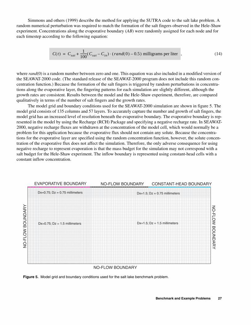
Simmons and others (1999) describe the method for applying the SUTRA code to the salt lake problem. A random numerical perturbation was required to match the formation of the salt fingers observed in the Hele-Shaw experiment. Concentrations along the evaporative boundary (AB) were randomly assigned for each node and for each timestep according to the following equation:

, (14)

where rand(0) is a random number between zero and one. This equation was also included in a modified version of the SEAWAT-2000 code. (The standard release of the SEAWAT-2000 program does not include this random con-centration function.) Because the formation of the salt fingers is triggered by random perturbations in concentra-tions along the evaporative layer, the fingering patterns for each simulation are slightly different, although the growth rates are consistent. Results between the model and the Hele-Shaw experiment, therefore, are compared qualitatively in terms of the number of salt fingers and the growth rates.

The model grid and boundary conditions used for the SEAWAT-2000 simulation are shown in figure 5. The model grid consists of 135 columns and 57 layers. To accurately capture the number and growth of salt fingers, the model grid has an increased level of resolution beneath the evaporative boundary. The evaporative boundary is rep-resented in the model by using the Recharge (RCH) Package and specifying a negative recharge rate. In SEAWAT-2000, negative recharge fluxes are withdrawn at the concentration of the model cell, which would normally be a problem for this application because the evaporative flux should not contain any solute. Because the concentra-tions for the evaporative layer are specified using the random concentration function, however, the solute concen-tration of the evaporative flux does not affect the simulation. Therefore, the only adverse consequence for using negative recharge to represent evaporation is that the mass budget for the simulation may not correspond with a salt budget for the Hele-Shaw experiment. The inflow boundary is represented using constant-head cells with a constant inflow concentration.

C t( ) Csat1

100--------- Csat Cin–( ) rand 0( ) 0.5–( ) milligrams per liter⋅+=

EVAPORATIVE BOUNDARY CONSTANT-HEAD BOUNDARYNO-FLOW BOUNDARY

NO

-FLO

W B

OU

ND

AR

Y

NO-FLOW BOUNDARY

NO

-FLO

W B

OU

ND

AR

Y

Dx=0.75; z = 0.75 millimetersD

D Dx=0.75; z = 1.5 millimeters D Dx=1.5; z = 1.5 millimeters

D Dx=1.5; z = 0.75 millimeters

Figure 5. Model grid and boundary conditions used for the salt lake benchmark problem.


The SEAWAT-2000 model was run for 24,000 seconds (400 minutes) using 60-second transport timesteps. The variable-density flow equation was solved using the PCG solver, and the implicit finite-difference method was used with the GCG Package to solve the transport equation. The name file used for the simulation is as follows:

#GLO PROCESS OUTPUT FILES

GLOBAL 6 saltlake.glo

LIST 7 saltlake.lst

#

#VDF PROCESS INPUT AND OUTPUT FILES

VDF 20 saltlake.vdf

BAS6 1 saltlake.bas

DIS 23 saltlake.dis

BCF6 11 saltlake.bcf

RCH 18 saltlake.rch

OC 22 saltlake.oc

PCG 19 saltlake.pcg

DATA(BINARY) 50 saltlake.cbb

DATA(BINARY) 30 saltlake.hds

#

#IMT PROCESS INPUT FILES

BTN 41 saltlake.btn

ADV 42 saltlake.adv

DSP 43 saltlake.dsp

SSM 44 saltlake.ssm

GCG 45 saltlake.gcg

The salt lake problem represents a complex system of salt fingers that form, descend, and then coalesce due to the larger-scale flow system. Although the results from SEAWAT-2000 are not identical with the results from the Hele-Shaw experiment, SEAWAT-2000 seems capable of representing the growth rate and number of salt fingers (fig. 6). In the experiment and model, six or seven salt fingers are initially produced, of which only two persist. The rate of descent is similar for both the experiment and model.

Rotation of Three Immiscible Fluids

A benchmark problem involving the rotating movement of three immiscible fluids was proposed as a test for verifying the density-dependent flow component of ground-water codes (Mark Bakker, University of Georgia, written commun., 2003). The problem consists of a cross-sectional box filled with three fluids of different densities. The initial boundaries between the fluids are not horizontal, and thus, the fluids rotate. There are two cases of this problem, one for symmetric rotational flow and one for asymmetric rotational flow. SEAWAT-2000 was used to simulate both cases of the problem. Simulated velocities at the onset of rotation are compared with velocities obtained using an analytical solution (Mark Bakker, University of Georgia, written commun., 2003).

The problem description is shown in figure 7, and values for aquifer geometry and properties are given in table 4. The interfaces between the three fluids are straight and slope down and to the right. The aquifer and fluids are assumed to be incompressible, and the effects of concentration on fluid viscosity are assumed to be negligible. The freshwater hydraulic conductivity is homogeneous and isotropic. Symmetric rotational flow results when the density for the middle fluid (ρ2) is set as the average of the two outer fluids (ρ1 and ρ3). Asymmetric rotational flow occurs for all other values for ρ2. A constant-head boundary is assigned to one of the corner cells to improve convergence of the flow solution.


A

B

C

D

E

F

G

H

EXPLANATION

11084 97

SALINITY,

IN GRAMS PER LITER

Figure 6. Contours of concentration from the SEAWAT-2000 simulation of the salt lake problem. Contour interval is 2 grams per liter.


Table 4. Geometry and aquifer properties for the rotation of three-immiscible fluids variable-density benchmark problem

[Modified from Mark Bakker (University of Georgia, written commun., 2003). Units: m, meter; kg/m3, kilogram per cubic meter; m/d, meter per day]

Geometry or aquifer property Variable Value

Length L 300 m

Aquifer thickness b 20 m

Density for fluid 1 ρ1 1,000 kg/m3

Density for fluid 2 ρ21,012.5 kg/m3 (symmetric case)1,005 kg/m3 (asymmetric case)

Density for fluid 3 ρ3 1,025 kg/m3

x distance for ρ1/ρ2 interface a1 40 m

x distance for ρ2/ρ3 interface a2 40 m

x midpoint position for ρ1/ρ2 interface x1 170 m

x midpoint position for ρ2/ρ3 interface x2 130 m

Freshwater hydraulic conductivity Kf 2 m/d

Porosity 0.2

ρ3

ρ2

ρ1

x2 x1

2a1

2a2

L

2b

xz

Constant-headboundary

Figure 7. Configuration for the rotation of fluids benchmark problem. (Mark Bakker, University of Georgia, written commun., 2003). Variables are defined in table 4.

θ


The symmetric and asymmetric cases of the rotational benchmark problem were run for 10,000 and 20,000 days, respectively. For both cases, flow was solved using the PCG Solver Package, and transport was solved using the MT3DMS TVD scheme and the GCG Solver. The name file used for both cases is shown here.

#GLO PROCESS OUTPUT FILESGLOBAL 6 rotate.gloLIST 7 rotate.lst##VDF PROCESS INPUT AND OUTPUT FILESVDF 20 rotate.vdfBAS6 1 rotate.basDIS 29 rotate.disLPF 11 rotate.lpfZONE 40 rotate.zoneOC 22 rotate.ocPCG 19 rotate.pcgDATA(BINARY) 50 rotate.cbbDATA(BINARY) 30 rotate.hds##IMT PROCESS INPUT FILESBTN 41 rotate.btnADV 42 rotate.advSSM 43 rotate.ssmGCG 44 rotate.gcg

The variable-density flow component of the SEAWAT-2000 program is verified by comparing the simulated horizontal velocities along the interface with the horizontal velocities calculated from the analytical solution. As the analytical solution is only valid for the initial velocity field, results from the SEAWAT-2000 simulation were saved after a short timestep of 0.001 day. The horizontal velocity, vh, is calculated for each point along the inter-faces using the following equation:

, (15)

where vx and vz are the flow velocities in the x and z directions, and –b/a is the slope of the interface. A simple computer program was written to calculate vh for each cell along the interface.

For the symmetric case, the horizontal velocities for the left interface compare almost exactly with the analytical solution (fig. 8), which verifies that SEAWAT accurately solves the variable-density flow equation for this particular problem. Although an analytical solution does not exist for later times, simulated interface configu-rations at 2,000 and 10,000 days are shown in figure 9. By definition, results from this analysis should be symmet-rical. Thus, the observed symmetry in model results further verifies the accuracy of the SEAWAT-2000 code.

For the asymmetric case, horizontal velocities for the right interface were compared with the analytical solu-tion and show close agreement (fig. 10). Simulated interface configurations at 2,000 and 20,000 days are shown in figure 11.

vh vx vzab---+=


-20

-15

-10

-5

0

5

10

15

20

-0.10 -0.05 0.00 0.05 0.10

HORIZONTAL VELOCITY OF LEFT INTERFACE, IN METERS PER DAY

SEAWAT-2000ANALYTICAL SOLUTION

Z L

OC

ATIO

N O

F L

EF

T IN

TE

RFA

CE

, IN

ME

TE

RS

100 200 300

X POSITION, IN METERS

-40

-20

0

Time = 2,000 days

Time = 10,000 days

Z P

OS

ITIO

N, I

N M

ET

ER

S

0

Figure 8. Initial horizontal velocity of the left interface for the symmetric case.

Figure 9. Interface positions for the symmetric case after 2,000 and 10,000 days.


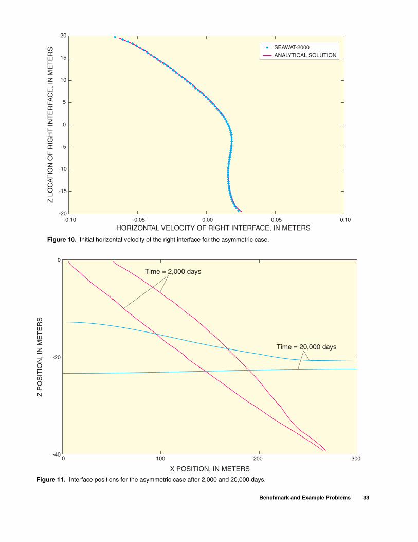
-20

-15

-10

-5

0

5

10

15

20

-0.10 -0.05 0.00 0.05 0.10

HORIZONTAL VELOCITY OF RIGHT INTERFACE, IN METERS

Z L

OC

ATIO

N O

F R

IGH

T IN

TE

RFA

CE

, IN

ME

TE

RS SEAWAT-2000

ANALYTICAL SOLUTION

Time = 20,000 days

Time = 2,000 days

100 200 300

X POSITION, IN METERS

-40

-20

0

Z P

OS

ITIO

N, I

N M

ET

ER

S

0

Figure 10. Initial horizontal velocity of the right interface for the asymmetric case.

Figure 11. Interface positions for the asymmetric case after 2,000 and 20,000 days.


Demonstration of Different Modes Using the Henry Problem

The SEAWAT-2000 program can be used in a number of different modes to represent constant-density or variable-density ground-water flow with or without solute transport (fig. 1). In this example, the Henry problem (Henry, 1964) is used to demonstrate the types of modes that are available in SEAWAT-2000. In the first simula-tion, SEAWAT-2000 is used to simulate the classic Henry problem, which involves variable-density ground-water flow coupled with solute transport (fig. 1E). The second simulation demonstrates the capability to simulate vari-able-density flow without solute transport (fig. 1C). This powerful new mode allows for relatively fast computer simulations if the fluid density field is not expected to change within a stress period. Lastly, an uncoupled variable-density flow and solute-transport simulation (fig. 1D) is performed to track a hypothetical contaminant through the interface between freshwater and saltwater. File types in the name file and options in the VDF input file are used to switch between these different modes.

The basic design of the Henry problem is shown in figure 12, and input variables are given in table 5. A constant flux of fresh ground water is applied to the left boundary at a rate (Qin) of 5.702 cubic meters per day with a concentration (Cin) equal to zero. A constant-head boundary is applied to the right side of the box to repre-sent hydrostatic (no vertical flow) conditions. The upper and lower boundaries are represented by the no-flow con-dition.

There has been some confusion in the literature about the molecular diffusion value (Dm) to use for the Henry problem. In the example presented here, Dm is specified as 1.62925 square meters per day, which is equiva-lent to case 1 in Guo and Langevin (2002). This corresponds with the molecular diffusion value originally used by Henry (1964).

SE

AW

ATE

R H

YD

RO

STA

TIC

DISTANCE, IN METERS

1.0 METER

0

Q, C

inin

1 20

No-flow boundary

Figure 12. Boundary conditions and dimensions for the Henry problem. Variables are defined in table 5.


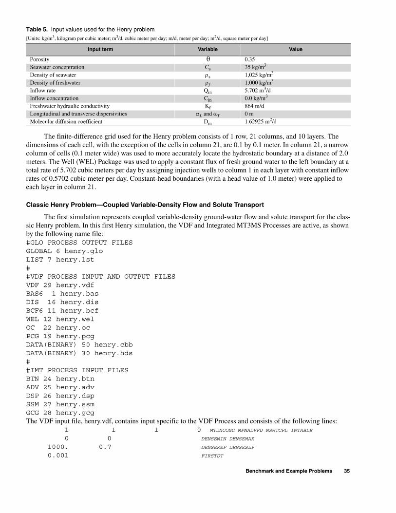
The finite-difference grid used for the Henry problem consists of 1 row, 21 columns, and 10 layers. The dimensions of each cell, with the exception of the cells in column 21, are 0.1 by 0.1 meter. In column 21, a narrow column of cells (0.1 meter wide) was used to more accurately locate the hydrostatic boundary at a distance of 2.0 meters. The Well (WEL) Package was used to apply a constant flux of fresh ground water to the left boundary at a total rate of 5.702 cubic meters per day by assigning injection wells to column 1 in each layer with constant inflow rates of 0.5702 cubic meter per day. Constant-head boundaries (with a head value of 1.0 meter) were applied to each layer in column 21.

Classic Henry Problem—Coupled Variable-Density Flow and Solute Transport

The first simulation represents coupled variable-density ground-water flow and solute transport for the clas-sic Henry problem. In this first Henry simulation, the VDF and Integrated MT3MS Processes are active, as shown by the following name file:#GLO PROCESS OUTPUT FILESGLOBAL 6 henry.gloLIST 7 henry.lst##VDF PROCESS INPUT AND OUTPUT FILESVDF 29 henry.vdfBAS6 1 henry.basDIS 16 henry.disBCF6 11 henry.bcfWEL 12 henry.welOC 22 henry.ocPCG 19 henry.pcgDATA(BINARY) 50 henry.cbbDATA(BINARY) 30 henry.hds##IMT PROCESS INPUT FILESBTN 24 henry.btnADV 25 henry.advDSP 26 henry.dspSSM 27 henry.ssmGCG 28 henry.gcgThe VDF input file, henry.vdf, contains input specific to the VDF Process and consists of the following lines: 1 1 1 0 MTDNCONC MFNADVFD NSWTCPL IWTABLE 0 0 DENSEMIN DENSEMAX 1000. 0.7 DENSEREF DENSESLP 0.001 FIRSTDT

Table 5. Input values used for the Henry problem

[Units: kg/m3, kilogram per cubic meter; m3/d, cubic meter per day; m/d, meter per day; m2/d, square meter per day]

Input term Variable Value

Porosity 0.35Seawater concentration Cs 35 kg/m3

Density of seawater ρs 1,025 kg/m3

Density of freshwater ρf 1,000 kg/m3

Inflow rate Qin 5.702 m3/dInflow concentration Cin 0.0 kg/m3

Freshwater hydraulic conductivity Kf 864 m/dLongitudinal and transverse dispersivities αL and αT 0 mMolecular diffusion coefficient Dm 1.62925 m2/d

θ


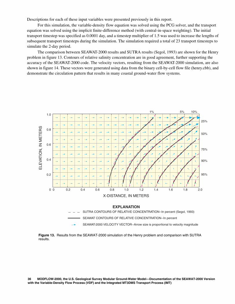
Descriptions for each of these input variables were presented previously in this report.For this simulation, the variable-density flow equation was solved using the PCG solver, and the transport

equation was solved using the implicit finite-difference method (with central-in-space weighting). The initial transport timestep was specified as 0.0001 day, and a timestep multiplier of 1.5 was used to increase the lengths of subsequent transport timesteps during the simulation. The simulation required a total of 23 transport timesteps to simulate the 2-day period.

The comparison between SEAWAT-2000 results and SUTRA results (Segol, 1993) are shown for the Henry problem in figure 13. Contours of relative salinity concentration are in good agreement, further supporting the accuracy of the SEAWAT-2000 code. The velocity vectors, resulting from the SEAWAT-2000 simulation, are also shown in figure 14. These vectors were generated using data from the binary cell-by-cell flow file (henry.cbb), and demonstrate the circulation pattern that results in many coastal ground-water flow systems.

0 0.2 0.4 0.6 0.8 1.0 1.2 1.4 1.6 1.8 2.0

X-DISTANCE, IN METERS

EXPLANATIONSUTRA CONTOURS OF RELATIVE CONCENTRATION--In percent (Segol, 1993)

SEAWAT CONTOURS OF RELATIVE CONCENTRATION--In percent

1% 5% 10%

25%

50%

75%

90%

95%

SEAWAT-2000 VELOCITY VECTOR--Arrow size is proportional to velocity magnitude

ELE

VAT

ION

, IN

ME

TE

RS

1.0

0.8

0.6

0.4

0.2

0

Figure 13. Results from the SEAWAT-2000 simulation of the Henry problem and comparison with SUTRA results.


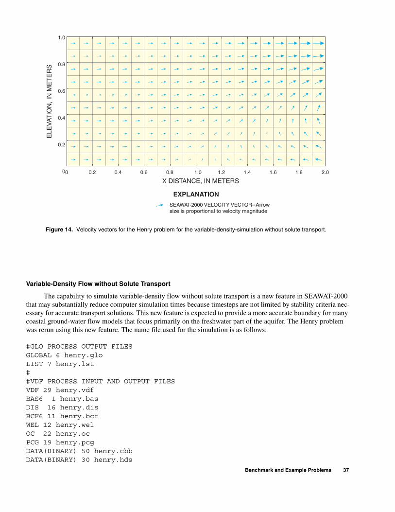
Variable-Density Flow without Solute Transport

The capability to simulate variable-density flow without solute transport is a new feature in SEAWAT-2000 that may substantially reduce computer simulation times because timesteps are not limited by stability criteria nec-essary for accurate transport solutions. This new feature is expected to provide a more accurate boundary for many coastal ground-water flow models that focus primarily on the freshwater part of the aquifer. The Henry problem was rerun using this new feature. The name file used for the simulation is as follows:

#GLO PROCESS OUTPUT FILESGLOBAL 6 henry.gloLIST 7 henry.lst##VDF PROCESS INPUT AND OUTPUT FILESVDF 29 henry.vdfBAS6 1 henry.basDIS 16 henry.disBCF6 11 henry.bcfWEL 12 henry.welOC 22 henry.ocPCG 19 henry.pcgDATA(BINARY) 50 henry.cbbDATA(BINARY) 30 henry.hds

EXPLANATION

SEAWAT-2000 VELOCITY VECTOR--Arrowsize is proportional to velocity magnitude

0 0.2 0.4 0.6 0.8 1.0 1.2 1.4 1.6 1.8 2.0

X DISTANCE, IN METERS

ELE

VAT

ION

, IN

ME

TE

RS

1.0

0.8

0.6

0.4

0.2

0

Figure 14. Velocity vectors for the Henry problem for the variable-density-simulation without solute transport.


For this simulation, solute transport is excluded as shown by the lack of MT3DMS input files in the name file. However, the presence of the VDF file type in the name file activates the VDF Process. Fluid densities for this problem are entered by specifying the solute concentrations from the previous simulation in the VDF input file and using the equation of state to convert the concentrations to fluid density (INDENSE = 2; DENSEREF = 1000; DENSESLP = 0.7). The VDF file used for this simulation is as follows:#VDF input file for Henry problem without solute transport 0 1 1 0 MTDNCONC MFNADVFD NSWTCPL IWTABLE 0 0 DENSEMIN DENSEMAX 1000. 0.7 DENSEREF DENSESLP 0.001 FIRSTDT 2INTERNAL 1 (5f12.2) 3 Concentration layer 1 1.9646E-05 5.2036E-05 1.3054E-04 3.1624E-04 7.4324E-04 1.6935E-03 3.7324E-03 7.9333E-03 1.6216E-02 3.1791E-02 5.9666E-02 0.1071 0.1838 0.3024 0.4783 0.7314 1.081 1.623 2.117 3.794 4.203 INTERNAL 1 (5f12.2) 3 Concentration layer 2 2.3280E-05 6.2549E-05 1.6022E-04 3.9784E-04 9.6081E-04 2.2537E-03 5.1188E-03 1.1218E-02 2.3629E-02 4.7679E-02 9.1892E-02 0.1689 0.2961 0.4964 0.7997 1.248 1.901 2.891 4.304 7.412 8.023 INTERNAL 1 (5f12.2) 3 Concentration layer 3 3.0673E-05 8.4188E-05 2.2223E-04 5.7113E-04 1.4306E-03 3.4839E-03 8.2138E-03 1.8660E-02 4.0647E-02 8.4494E-02 0.1670 0.3129 0.5561 0.9404 1.523 2.381 3.635 5.484 8.254 12.23 12.78 INTERNAL 1 (5f12.2) 3 Concentration layer 4 4.1954E-05 1.1779E-04 3.2075E-04 8.5319E-04 2.2146E-03 5.5878E-03 1.3633E-02 3.1971E-02 7.1619E-02 0.1523 0.3059 0.5786 1.030 1.733 2.772 4.259 6.339 9.202 12.96 16.96 17.38 INTERNAL 1 (5f12.2) 3 Concentration layer 5 5.7015E-05 1.6367E-04 4.5903E-04 1.2609E-03 3.3825E-03 8.8161E-03 2.2184E-02 5.3499E-02 0.1227 0.2655 0.5386 1.020 1.801 2.981 4.655 6.923 9.876 13.55 17.70 21.33 21.66 INTERNAL 1 (5f12.2) 3 Concentration layer 6 7.5209E-05 2.2046E-04 6.3558E-04 1.7988E-03 4.9748E-03 1.3363E-02 3.4605E-02 8.5629E-02 0.2005 0.4401 0.8975 1.692 2.944 4.756 7.187 10.25 13.91 18.00 22.10 25.41 26.06 INTERNAL 1 (5f12.2) 3 Concentration layer 7 9.5069E-05 2.8406E-04 8.3960E-04 2.4415E-03 6.9448E-03 1.9190E-02 5.1063E-02 0.1295 0.3093 0.6871 1.405 2.627 4.486 7.036 10.24


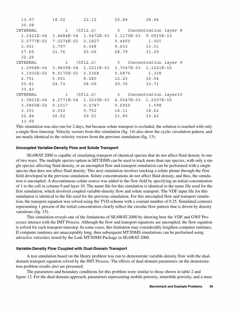
13.97 18.02 22.12 25.89 28.94 30.08 INTERNAL 1 (5f12.2) 3 Concentration layer 8 1.1421E-04 3.4684E-04 1.0472E-03 3.1175E-03 9.0915E-03 2.5777E-02 7.0374E-02 0.1827 0.4450 1.001 2.051 3.797 6.348 9.653 13.51 17.65 21.76 25.56 28.79 31.29 32.26 INTERNAL 1 (5f12.2) 3 Concentration layer 9 1.2958E-04 3.9835E-04 1.2221E-03 3.7047E-03 1.1021E-02 3.1932E-02 8.9172E-02 0.2368 0.5876 1.338 2.751 5.051 8.280 12.23 16.54 20.81 24.73 28.09 30.76 32.71 33.43 INTERNAL 1 (5f12.2) 3 Concentration layer10 1.3821E-04 4.2771E-04 1.3239E-03 4.0547E-03 1.2207E-02 3.5860E-02 0.1017 0.2747 0.6929 1.598 3.301 6.032 9.752 14.11 18.62 22.84 26.52 29.51 31.80 33.42 33.99 This simulation was also run for 2 days, but because solute transport is excluded, the solution is reached with only a single flow timestep. Velocity vectors from this simulation (fig. 14) also show the cyclic circulation pattern, and are nearly identical to the velocity vectors from the previous simulation (fig. 13).

Uncoupled Variable-Density Flow and Solute Transport

SEAWAT-2000 is capable of simulating transport of chemical species that do not affect fluid density in one of two ways. The multiple species option in MT3DMS can be used to track more than one species, with only a sin-gle species affecting fluid density, or an uncoupled flow and transport simulation can be performed with a single species that does not affect fluid density. This next simulation involves tracking a solute plume through the flow field developed in the previous simulation. Solute concentrations do not affect fluid density, and thus, the simula-tion is uncoupled. A discontinuous solute source was added to the flow field by specifying an initial concentration of 1 to the cell in column 9 and layer 10. The name file for this simulation is identical to the name file used for the first simulation, which involved coupled variable-density flow and solute transport. The VDF input file for this simulation is identical to the file used for the previous simulation. For this uncoupled flow and transport simula-tion, the transport equation was solved using the TVD scheme with a courant number of 0.25. Simulated contours representing 1 percent of the initial concentration clearly reflect the circular flow pattern that is driven by density variations (fig. 15).

This simulation reveals one of the limitations of SEAWAT-2000 by showing how the VDF and GWF Pro-cesses interact with the IMT Process. Although the flow and transport equations are uncoupled, the flow equation is solved for each transport timestep. In some cases, this limitation may considerably lengthen computer runtimes. If computer runtimes are unacceptably long, then subsequent MT3DMS simulations can be performed using advective velocities stored by the Link MT3DMS Package in SEAWAT-2000.

Variable-Density Flow Coupled with Dual-Domain Transport

A test simulation based on the Henry problem was run to demonstrate variable-density flow with the dual-domain transport equation solved by the IMT Process. The effects of dual domain parameters on the demonstra-tion problem results also are presented.

The parameters and boundary conditions for this problem were similar to those shown in table 2 and figure 12. For the dual-domain approach, parameters representing mobile porosity, immobile porosity, and a mass


transfer coefficient must be assigned. Mobile porosity was initially set to 30 percent, immobile porosity was ini-tially set to 10 percent, and total porosity of the porous media was, therefore, 40 percent. The mass transfer coeffi-cient was initially set to 1.0 day-1. A transition zone between freshwater and saltwater developed due to advection in the mobile domain and diffusive mass transfer between the mobile and immobile domains. The resulting salin-ity distribution was roughly the same as the salinity distribution that was simulated for the classic Henry problem (fig. 13).

To examine the effects of dual-domain parameters on the transition zone between freshwater and saltwater, an observation well was placed in layer 10, row 1, and column 20 of the test problem. The observation well was activated using the BTN Package (Zheng and Wang, 1999, pg. 111). Mobile porosity (θm), immobile porosity (θim), and the mass transfer coefficient (ζ) were individually varied from their initial values while rerunning the test problem and tracking salinity results (fig. 16). Mobile porosity was assigned values of 0.1, 0.3, and 0.8 while immobile porosity and the mass transfer coefficient were kept at initial values. As expected, saltwater moved more quickly through the observation well with smaller values of mobile porosity (fig. 16A). Changing immobile poros-ity from 0.1 to 0.6 while keeping mobile porosity and the mass transfer coefficient at initial values had little effect on the problem results (fig. 16B). Saltwater also moved more quickly through the observation well with a smaller value (1 x 10-5) of the mass transfer coefficient (fig. 16C) because there was less exchange between the mobile and immobile domains.

EXPLANATION

0 0.2 0.4 0.6 0.8 1.0 1.2 1.4 1.6 1.8 2.0

X DISTANCE, IN METERS

0.005 day

0.01 day

0.05 day

CONTOUR REPRESENTING 1 PERCENTOF INITIAL CONCENTRATION

INITIAL CONCENTRATION SET TO 1

SEAWAT-2000 VELOCITY VECTOR--Arrowsize is proportional to velocity magnitude

ELE

VAT

ION

, IN

ME

TE

RS

1.0

0.8

0.6

0.4

0.2

0

Figure 15. Results from uncoupled simulation of variable-density flow and solute transport. Contours represent 1 percent of the initial concentration.


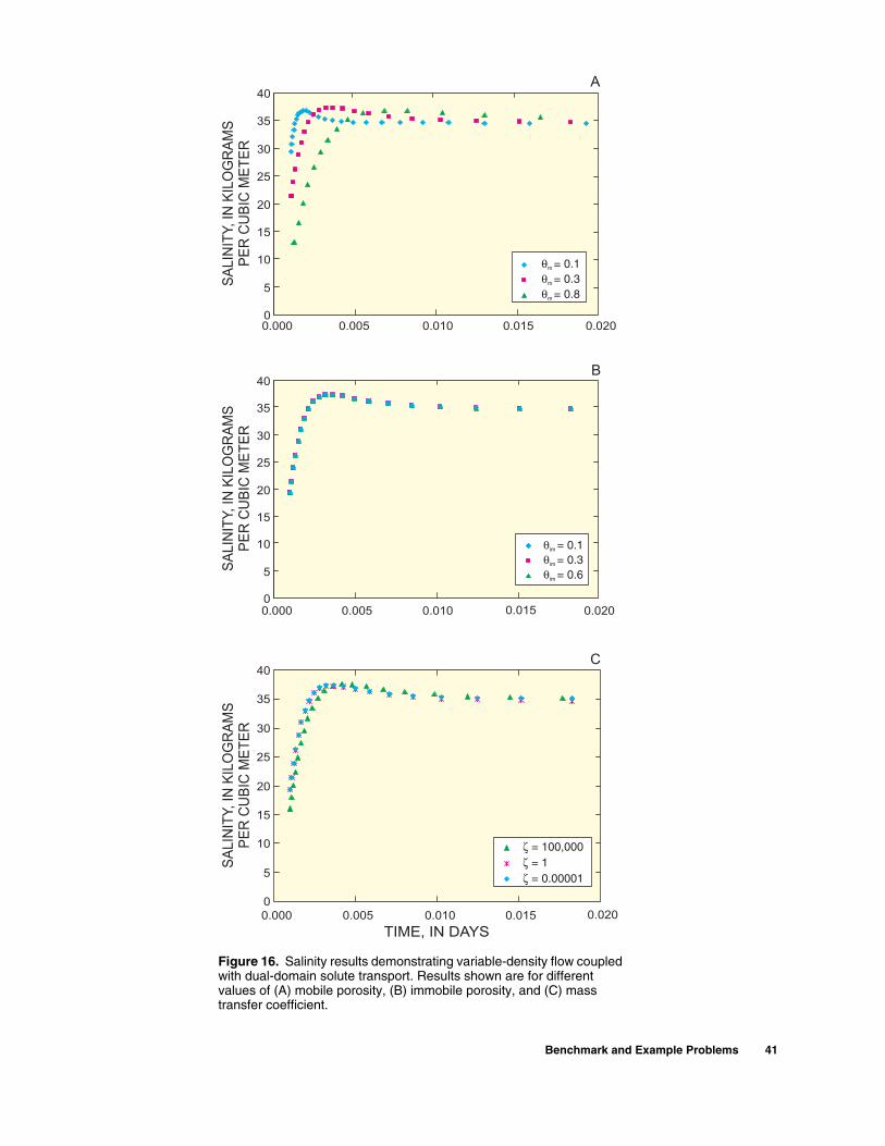
0

5

10

15

20

25

30

35

40

0.000 0.005 0.010 0.015 0.020

SA

LIN

ITY,

INK

ILO

GR

AM

S

PE

RC

UB

ICM

ET

ER

θm = 0.1θm = 0.3θm = 0.8

0

5

10

15

20

25

30

35

40

0.000 0.005 0.010 0.015 0.020

SA

LIN

ITY,IN

KIL

OG

RA

MS

PE

RC

UB

ICM

ET

ER

0

5

10

15

20

25

30

35

40

0.000 0.005 0.010 0.015 0.020

TIME, IN DAYS

SA

LIN

ITY,

INK

ILO

GR

AM

S

PE

RC

UB

ICM

ET

ER

A

B

C

θim = 0.1θim = 0.3θim = 0.6

ζ = 100,000ζ = 1ζ = 0.00001

Figure 16. Salinity results demonstrating variable-density flow coupled with dual-domain solute transport. Results shown are for different values of (A) mobile porosity, (B) immobile porosity, and (C) mass transfer coefficient.


REFERENCES CITED

Anderman, E.R., and Hill, M.C., 2000, MODFLOW-2000, the U.S. Geological Survey modular ground-water model − Documentation of the hydrogeologic-unit flow (HUF) package: U.S. Geological Survey Open-File Report 00-342, 89 p.

Feehley, E.C., Zheng, Chunmiao, and Molz, F.J., 2000, A dual-domain mass transfer approach for modeling solute transport in heterogeneous aquifers: Application to the macrodispersion experiment (MADE) site: Water Resources Research, v. 36, no. 9, p. 2501-2515.

Guo, Weixing, and Bennett, G.D., 1998, Simulation of saline/fresh water flows using MODFLOW; in E. Poeter and others, Proceedings of the MODFLOW ’98 Conference, Golden, Colo., v. 1, p. 267-274.

Guo, Weixing, and Langevin, C.D., 2002, User’s guide to SEAWAT: A computer program for simulation of three-dimensional variable-density ground-water flow: U.S. Geological Survey Techniques of Water-Resources Investigations, book 6, chap. A7, 77 p.

Harbaugh, A.W., 1995, Direct solution package based on alternating diagonal ordering for the U.S. Geological Survey modular finite-difference ground-water flow model: U.S. Geological Survey Open-File Report 95-288, 46 p.

Harbaugh, A.W., Banta, E.R., Hill, M.C., and McDonald, M.G., 2000, MODFLOW-2000, the U.S. Geological Survey modular ground-water model – User guide to modularization concepts and the ground-water flow process: U.S. Geological Survey Open-File Report 00-92, 121 p.

Henry, H.R., 1964, Effects of dispersion on salt encroachment in coastal aquifers: U.S. Geological Survey Water–Supply Paper 1613–C, p. C71-C84.

Hill, M.C., 1990, Preconditioned conjugate-gradient 2 (PCG2), a computer program for solving groundwater equations: U.S. Geological Survey Water-Resources Investigations Report 90-4048, 43 p.

Hill, M.C., Banta, E.R., Harbaugh, A.W., and Anderman, E.R., 2000, MODFLOW-2000, the U.S. Geological Survey modular ground-water model – User guide to the observation, sensitivity, and parameter estimation processes and three post-processing programs: U.S. Geological Survey Open-File Report 00-184, 209 p.

Hornberger, G..Z., Konikow, L.F., and Harte, P.T., 2002, Simulating solute transport across horizontal-flow barriers using the MODFLOW ground-water transport process: U.S. Geological Survey Open-File Report 02-52, 28 p.

Hsieh, P.A., and Freckleton, J.R., 1993, Documentation of a computer program to simulate horizontal flow barriers using the U.S. Geological Survey’s modular three-dimensional finite-difference ground-water flow

42 MODFLOW-2000, the U.S. Geological Survey Modular Grounwith the Variable-Density Flow Process (VDF) and the Integrated M

model: U.S. Geological Survey Open-File Report 92-477, 32 p.

Konikow, L.F., Sanford, W.E., and Campbell, P.J., 1997, Constant-concentration boundary condition: Lessons from the HYDROCOIN variable-density groundwater benchmark problem: Water Resources Research, v. 33, no. 10, p. 2253-2261.

Langevin, C.D., and Guo, Weixing, 1999, Improvements to SEAWAT, a variable-density modeling code [abs.]: in EOS Transactions, v. 80, no. 46., p. F-373.

Leake, S.A., and Prudic, D.E., 1991, Documentation of a computer program to simulate aquifer-system compaction using the finite-difference ground-water flow model: U.S. Geological Survey Techniques of Water Resources Investigations, book 6, chap. A2, p. 68.

McDonald, M.G.., and Harbaugh, A.W., 1988, A modular three-dimensional finite-difference ground-water flow model: U.S. Geological Survey Techniques of Water Resources Investigations, book 6, chap. A1, 586 p.

Mehl, S.W., and Hill, M.C., 2001, MODFLOW-2000, the U.S. Geological Survey modular ground-water model – User guide to the link-AMG (LMG) package for solving matrix equations using an algebraic multigrid solver: U.S. Geological Survey Open-File Report 01-177, 33 p.

Segol, Genevieve, 1993, Classic groundwater simulations: Proving and improving numerical models: Englewood Cliffs, N.J., PTR Prentice Hall, 531 p.

Simmons, C.T., Narayan, K.A., and Wooding, R.A., 1999, On a test case for density-dependent groundwater flow and solute transport models: The salt lake problem: Water Resources Research, v. 35, no. 12, p. 3607-3620.

Voss, C.I., and Souza, W.R, 1987, Variable density flow and solute transport simulation of regional aquifers containing a narrow freshwater-saltwater transition zone: Water Resources Research, v. 23, no. 10, p. 1851-1866.

Wooding, R.A., Tyler, S.W., and White, Ian, 1997a, Convection in groundwater below an evaporating salt lake, 1, Onset of instability: Water Resources Research, v. 33, no. 6, p. 1199-1217.

Wooding, R.A., Tyler, S.W., White, Ian, and Anderson, P.A., 1997b, Convection in groundwater below an evaporating salt lake, 2, Evolution of fingers or plumes: Water Resources Research, v. 33, no. 6, p. 1219-1228.

Zheng, Chunmiao, 1996, MT3D-A modular three-dimensional transport model for simulation of advection, dispersion and chemical reactions of contaminants in groundwater systems: S.S. Papadopulos & Associates, Inc., Bethesda, Md.

d-Water Model—Documentation of the SEAWAT-2000 Version T3DMS Transport Process (IMT)

Zheng, Chunmiao, and Gorelick, S.M., 2001, Analysis of solute transport and remediation in flow fields influenced by decimeter-scale preferential flow paths: Proceedings of MODFLOW 2001 and other Modeling Odysseys, September 11-14, 2001, International Ground-water Modeling Center (IGWMC), Colorado School of Mines, Golden, Colo., v. 1, p. 11.

Zheng, Chunmiao, Hill, M.C., and Hsieh, P.A., 2001, MODFLOW-2000, the U.S. Geological Survey modular ground-water model – User guide to the LMT6 package, the linkage with MT3Dms for multi-species mass transport modeling: U.S. Geological Survey Open-File Report 01-82, 43 p.

Zheng, Chunmiao, and Wang, P.P., 1998, MT3DMS, A modular three-dimensional multispecies transport model for simulation of advection, dispersion and chemical reactions of contaminants in groundwater systems: Vicksburg, Miss., Waterways Experiment Station, U.S. Army Corps of Engineers.

Zheng, Chunmiao, and Wang, P.P., 1999, MT3DMS—A modular three-dimensional multispecies transport model for simulation of advection, dispersion and chemical reactions of contaminants in ground-water systems; documentation and user’s guide: Jacksonville, Fla., U.S. Army Corps of Engineers Contract Report SERDP-99-1.

References Cited 43

modflow-2000, the u.s. geological survey modular … · introduction 1 modflow-2000, the u.s....

Documents