modflow groundwater modeling us army, fort … · modflow groundwater modeling us army, fort...

1

MODFLOW GROUNDWATER MODELING

US ARMY, FORT MONMOUTH Main Post and Charles Wood Areas

June 10, 2010

1.0 INTRODUCTION

Based upon data provided by Fort Monmouth (Fort), Brinkerhoff Environmental Services, Inc. (Brinkerhoff) developed and refined sitewide groundwater flow models for the Main Post and Charles Wood areas. The models were developed with Visual MODFLOW, using monitoring well casing and groundwater elevation data for approximately 200 wells. The MODFLOW program is a three (3)-dimensional groundwater flow simulation software package developed by the United States Geological Survey (USGS). Visual MODFLOW denotes an aftermarket version of the software enhanced by Schlumberger Canada Limited via a graphical user interface (GUI) and other program enhancements. MODFLOW is generally considered the most widely used groundwater simulation software in the industry. Development of the models included the review and incorporation of significant geologic boundaries based upon soil boring logs and aquifer testing data (i.e., slug tests) maintained by the Fort. The soil boring information was supplemented, where appropriate, by published geologic data. The models also utilized base map topographic information and other pertinent geographic information system (GIS) data for Main Post and Charles Wood areas provided by the Fort in AutoCAD or GIS-compatible formats. Development of the models supports the Fort Monmouth internal efforts in understanding groundwater flow across the Main Post and Charles Wood areas and aids planning for future monitoring well installations and delineation of groundwater contaminant plumes. As the groundwater models simulate groundwater flow conditions in these areas, they will also be used for contaminant transport modeling and thereby provide greater understanding of the factors affecting groundwater contamination migration and support for the development of groundwater Classification Exception Areas (CEAs). This document provides a generalized description of the modeling process and summarizes key parameters used in the development of the groundwater flow models.

2

2.0 GROUNDWATER MODEL CREATION

2.1 Conceptual Model The development of a groundwater model begins with the review and evaluation of geological resources and maps to create a conceptual model. Key items used for this purpose include the following resources:

Site-Specific Reports and Boring Logs (Basewide); USGS Topographic Maps; GIS System Data; and Published Geology Resources.

2.1.1 Site-Specific Reports and Boring Logs Soil boring logs and site-specific environmental investigation reports provided by the Fort were reviewed to the extent necessary to contribute to the conceptual models. 2.1.2 United States Geological Survey (USGS) Topographic Maps Topographic maps were used in characterizing the ground surface elevations in the area surrounding the Fort property. 2.1.3 Geographic Information System (GIS) Data GIS data maintained by the Fort provide ground surface topography information, locations of surface water bodies, base maps, and other relevant data. 2.1.4 Published Geologic Resources Published geologic resources were utilized to provide regional geology information and were consulted in various instances to evaluate model design and input parameters. A summary of regional geology is provided in Section 3.0. 2.2 Field Data Gathering 2.2.1 Calculated Groundwater Elevations The primary data utilized in the groundwater model creation are depth to water and calculated groundwater elevations based upon the Fort's database of surveyed monitoring well locations and casing elevations. During the model development, anomalous groundwater elevation data points were evaluated for possible errors.

3

For example, this could include specific field conditions such as water ponding, which could result in localized groundwater mounding, or in the case of older survey data, use of an older benchmark system. In most cases, additional field and/or survey data were collected to ensure accurate data points. The Fort’s Standard Practice Procedure for the collection of well depth measurements is provided in Appendix I. A summary of the Fort's May 2009 Well Search, including both on-site and off-site wells, is included in Appendix II. Well locations on and around the Main Post and Charles Wood areas are shown on the Monitoring Well Location Maps provided in Appendix III. 2.2.2 Aquifer Testing Through the course of various contaminant investigations conducted by the Fort, aquifer testing was performed consisting primarily of rising head slug tests. Hydraulic conductivity data generated from these tests were compiled, evaluated, compared to literature values, and representative values were assigned to each layer in the model domain. A summary of hydraulic conductivities recorded for the Main Post Area is provided in Appendix IV. By virtue of its smaller size and other factors, fewer slug tests have been performed at the Charles Wood Area. Although values for individual slug tests were not readily available, it was reported in previous technical reports (Versar, CEA Information for Site CW-1 Report dated May 29, 2008) that the geometric mean for seven (7) slug tests performed for shallow wells (generally 12-13 foot depth) at Building 2567 was 25.8 feet/day. 2.2.3 Preliminary Tidal Evaluation As part of this project, Brinkerhoff performed a Preliminary Tidal Evaluation of select monitoring wells throughout the Main Post Area of the Fort. The study locations selected mutually by Brinkerhoff and representatives of the Fort were chosen to represent an overall profile of the Main Post area. On September 29, 2009, wireless “downhole” pressure transducers (data loggers) were placed into each of the 25 predetermined groundwater monitoring wells targeted for the study. Pressure data were collected for approximately 30 days. An optical water interface probe was utilized to obtain manual depth to water (DTW) measurements, which were collected prior to setting each data logger. The initial DTW value was later utilized to convert the head pressure values collected by the data loggers to actual groundwater elevations. Additionally, one (1) barometric pressure transducer (Baro-Diver) was employed to account for changes in barometric pressure during the evaluation.

4

Upon completion of the data collection period, data logger units were retrieved from the monitoring wells and the raw data were downloaded. Barometric pressure recordings and manual DTW readings were utilized to convert monitoring wellhead pressure data to groundwater elevations. Subsequent groundwater elevations were then plotted to determine which areas exhibit tidal influence. A complete data report for Monitoring Well M3MW07 is provided as a sample in Appendix V. Due to the extensive size of the resulting printouts, the data reports for all of the study wells are included on a CD-ROM located within that same appendix. Charts displaying groundwater elevations for the monitoring wells are included in Appendix VI. Tidal information from the USGS Shrewsbury River Tidal Gage and average rainfall data for the month of October 2009 from the National Oceanic and Atmospheric Administration (NOAA) Climatological Report were obtained and utilized for comparison purposes. Refer to Appendix VII. Included below in Table 1 is a listing of monitoring wells included in the study followed by a summarization of findings associated with each of the tidal evaluation areas.

Table 1 Summary of Tidal Evaluation Areas/Monitoring Wells

Tidal Evaluation Area Monitoring Wells M2 Landfill (FTMM-02*) M2MW02, M2MW03, M2MW04, M2MW09, and

M2MW15 M3 (FTMM-03*) and

M5 Landfill (FTMM- 05*) M3MW05, M3MW07, and M5MW19

M4 Landfill M4MW05, M4MW07 and M4MW10 M8 Landfill (FTMM-08*) M8MW22 and M8MW23

M12 Landfill (FTMM-12*) M12MW17, M12MW20, and M12MW24 M14 Landfill (FTMM-14*) M14MW20 and M14MW24

MP 18 Landfill (FTMM-18*) and Building 283 (FTMM-61*)

MP18MW25 and 283MW06

Buildings 80 (FTMM-56*) and 108 (FTMM-57*)

80MW02 and 108MW04

Building 296 (FTMM-54*) 296MW01 and 296MW06 Building 699 (FTMM-53*) 699MW15

Building 1122 (FTMM-59*) 1122MW01 *Fort Monmouth Installation Restoration Program (IRP) Name

M2 Landfill (FTMM-02) Groundwater Monitoring Wells M2MW02, M2MW03, M2MW04, M2MW09, and M2MW15 were utilized as part of the tidal evaluation within the M2 Landfill area. These monitoring wells were chosen to be representative of the conditions in relationship to the southwestern portion of Mill Creek as it traverses the Main Post area.

5

Tidal study data for the M2 Landfill area indicated varied degrees of tidal influence. In general, monitoring wells directly adjacent to Mill Creek (M2MW02, M2MW03 and M2MW09) exhibited the greatest amount of cyclical groundwater fluctuations; however, influence dissipated as the distance from Mill Creek increased. M2MW04 appeared to have identifiable yet minimal fluctuations associated with extreme high tides, while M2MW15 did not exhibit any noticeable influence. Additionally, groundwater fluctuations in tidally influenced wells appeared to be exaggerated during periods of heavy rainfall (October 15 through October 20, 2009) and is congruent with heavy rainfall amounts recorded by the National NOAA, Trenton, New Jersey, monitoring station during this period. M3 (FTMM-03) and M5 (FTMM-05) Landfills Groundwater Monitoring Wells M3MW05, M3MW07, and M5MW19 were utilized as part of the tidal evaluation within the M3 and M5 Landfill areas. Landfills M3 and M5 are located at the junction of Parkers Creek and Mill Creek. Monitoring Well M3MW07 exhibited a rhythmic cycle of groundwater fluctuations indicative of tidal influence. Monitoring Well M3MW05 also exhibited an underlying pattern of groundwater fluctuations which may be indicative of slight tidal influence; however, it appears the rise and fall of groundwater elevations in this monitoring well are the results of high susceptibility to rainfall infiltration. Monitoring Well M5MW19 is within the same general area as the two (2) previously mentioned groundwater monitoring wells; however, no indication of tidal influence was observed in the groundwater elevation data. Monitoring Well M5MW19 is approximately six-point-five (6.5) feet above mean sea level (MSL). Tidal study data indicate that groundwater elevations greater than four (4) feet above MSL typically exhibit limited tidal influence. M4 Landfill Groundwater Monitoring Wells M4MW05, M4MW07 and M4MW10 were utilized as part of the tidal evaluation within the M4 Landfill area. Landfill M4 is along the east side of Mill Creek to the south of the Mill Creek and Parkers Creek junction. Monitoring Well M4MW10, directly adjacent to Mill Creek, exhibited a rhythmic cycle of groundwater fluctuations indicative of tidal influence. Groundwater data collected for M4MW07, approximately 160 feet east of Mill Creek, did not appear to indicate tidal influence; however, subtle fluctuations corresponding with large rainfall events were apparent.

6

It is evident from the groundwater elevation data that M4MW07 is not tidally influenced. Presumably, this is due to the high topographic elevation at this location (six-point-five [6.5] feet above MSL). This location does, however, appear susceptible to irregular groundwater elevation changes caused by surface water permeation. M8 Landfill (FTMM-08) Groundwater Monitoring Wells M8MW22 and M8MW23 were utilized as part of the tidal evaluation within the M8 Landfill area. The M8 Landfill is along Parkers Creek at the northern edge of Main Post. Monitoring Well M8MW22 exhibited a rhythmic cycle of groundwater fluctuations indicative of tidal influence. Monitoring Well M8MW23 also exhibited an underlying pattern of groundwater fluctuations which may be indicative of slight tidal influence; however, it appears the more predominant groundwater elevation changes in M8MW23 are the result of rainfall infiltration. Although the groundwater elevations for M8MW23 are within the lower range where tidal influence is common, the significant distance (approximately 375 feet) from Parkers Creek appears to have muted the effect. M12 Landfill (FTMM-12) Groundwater Monitoring Wells M12MW17, M12MW20, and M12MW24 were utilized as part of the tidal evaluation within the M12 Landfill area. M12 Landfill is centrally located on the Main Post adjacent to Oceanport Creek. Groundwater Monitoring Wells M12MW17 and M12MW20 exhibited a rhythmic cycle of groundwater fluctuations indicative of tidal influence; however, M12M24, approximately 300 feet from Oceanport Creek and seven (7) feet above MSL, appeared to be outside of the tidal influence range. Tidal study data indicate that groundwater elevations greater than four (4) feet above MSL typically exhibit limited tidal influence. M14 Landfill (FTMM-14) Groundwater Monitoring Wells M14MW20 and M14MW24 were utilized as part of the tidal evaluation within the M14 Landfill area. Landfill M14 is located adjacent to Oceanport Creek. Although an underlying rhythmic cycle appears to be present at this location, fluctuations may represent changes in hydraulic gradient and not tidal fluctuations. These changes appear to be exaggerated at intervals of low tide when the difference is the greatest between the groundwater elevation in the well and the corresponding surface water. This effect appears to be muted around high tide when the difference is less significant.

7

MP18 Landfill (FTMM-18) and Building 283 (FTMM-61) Area Groundwater Monitoring Wells MP18MW25 and 283MW06 were utilized as part of the tidal evaluation for this area. This area is at the northern part of the Main Post and to the south of Parkers Creek. It is evident from the groundwater elevation data that Monitoring Wells MP18MW25 and 283MW06 are not tidally influenced. For 283MW06, this appears to be due to the high topographic elevation at this location and distance from Parkers Creek. This location does, however, appear susceptible to groundwater elevation changes caused by surface water permeation. For M8MW23, groundwater elevations are within the lower range where tidal influence is common, although the effect appears to be muted except during extreme high water events. Buildings 80 (FTMM-56) and 108 (FTMM-57) Area Groundwater Monitoring Wells 80MW02 and 108MW04 were utilized as part of the tidal evaluation for this area. This area is at the eastern portion of the Main Post between the open water portions of Parkers Creek and Oceanport Creek. Although tidal influence would be expected in close proximity to the surface water, rhythmic fluctuations indicative of such were not observed at these locations. Additionally, Monitoring Well 108MW04 groundwater elevation data indicate exaggerated groundwater fluctuations congruent with heavy rainfall amounts recorded during this period, indicating high susceptibility to surface water infiltration. Building 296 (FTMM-54) Area Groundwater Monitoring Wells 296MW01 and 296MW06 were utilized as part of the tidal evaluation at this location. Building 296 is south of Parkers Creek between the M8 and MP18 Landfills. Tidal influence does not appear evident in this area, although 296MW06 exhibits short-term tidal impact under extremely high water conditions. Additionally, groundwater elevation data indicate exaggerated groundwater fluctuations congruent with heavy rainfall amounts recorded during this period, indicating high susceptibility to surface water infiltration. Building 699 (FTMM-53) Area Groundwater Monitoring Well 699MW15 was utilized in the tidal evaluation to represent this area. This area is located centrally within the Main Post and is not near any surface water features; therefore, no tidal impact was anticipated.

8

It is evident from the groundwater elevation data that this area is not tidally influenced. This location does, however, appear susceptible to groundwater elevation changes caused by surface water permeation. Building 1122 (FTMM-59) Area Groundwater Monitoring Well 1122MW01 was utilized in the tidal evaluation to represent this area. This area is on the southern side of Mill Creek, between landfills M2 and M4. It is evident from the groundwater elevation data that this area is not tidally influenced. This location does, however, appear susceptible to groundwater elevation changes caused by surface water permeation. Summary Based upon the preliminary evaluation presented herein, the potential extent of tidal influence was determined. For simplicity, areas with groundwater elevations less than five (5) feet above MSL (based upon the MODFLOW output) are considered within the Primary Zone of potential tidal influence. Known wetlands and landfill areas were also included in a Secondary Zone due to low ground surface elevations typical for wetlands and the disturbed nature of the landfill areas. The mapping of these zones is intended to guide the decision-making process regarding potential tidal influence when evaluating contamination sites. Areas outside of these zones are not likely to be tidally influenced; areas within require a site-specific evaluation as needed. In certain monitoring wells, exaggerated groundwater fluctuations were observed which appear to be related to heavy rainfall amounts recorded during the test period. There are a variety of natural and man-made conditions which could produce this effect. It is important, therefore, to consider such a possibility when evaluating groundwater elevation measurements. A map of the estimated extent of tidal influence is included in Appendix VII. 2.3 Model Calibration and Limitations 2.3.1 Model Calibration Process Calibration of the groundwater flow model is based upon the comparison of model simulation results and observed field data, particularly groundwater elevation (head) measurements. This is generally a trial-and-error process, with the results of each parameter change evaluated and the next trial guided by professional judgment.

9

The goal for calibration is to identify values for hydrologic properties that provide a reasonable fit between the simulated water levels and those measured at the site.

2.3.2 Model Limitations A groundwater flow model is designed as an approximation of an actual groundwater system. The accuracy of the simulated water levels and flow is proportionate to the accuracy with which the actual groundwater system is represented by the model components which, in turn, is based upon the data available to guide the program inputs. In general, model accuracy is increased as the area represented by the model decreases as long as the amount and quality of field data available also increase. Therefore, the development of site-specific localized "daughter" models is recommended, as they will improve upon the basewide groundwater flow models being presented herein through evaluation of localized flow patterns in the affected areas.

10

3.0 REGIONAL GEOLOGY

Geologic conditions in the area of the Fort were previously summarized by Versar Inc. (Versar, 2003) and are adapted herein. 3.1 Summary of Regional Geology The Fort lies within the Outer Coastal Plain subprovince of the New Jersey section of the Atlantic Coastal Plain physiographic province, which generally consists of a seaward-dipping wedge of unconsolidated sediments including interbedded clay, silt, sand, and gravel. To the northwest is the boundary between the Outer and Inner Coastal Plains, marked by a line of hills extending southwest from the Atlantic Highlands overlooking Sandy Hook Bay to a point southeast of Freehold, New Jersey, and then across the state to the Delaware Bay. These formations of clay, silt, sand, and gravel formations were deposited on Precambrian and lower Paleozoic rocks and typically strike northeast-southwest, with a dip that ranges from 10 – 60 feet per mile. Coastal Plain sediments date from the Cretaceous through the Quaternary Periods and are predominantly derived from deltaic, shallow marine, and continental shelf environments. The Fort is located within the outer fringe of the Atlantic Coastal Plain Physiographic Province of New Jersey, approximately 20 miles south of Raritan Bay. This province is characterized by a wedge-shaped mass of unconsolidated to semiconsolidated marine, marginal marine, and nonmarine deposits of clay, silt, sand, and gravel. These sediments range in age from Cretaceous to Holocene and lie unconformably on pre-Cretaceous bedrock consisting of metamorphic schists and gneiss, with local occurrences of basalts, sandstone, and shale (Zapecza, 1984). These sediments trend northeast-southwest and dip southeast toward the Atlantic Ocean. These sediments thicken southeastward from the Piedmont-Coastal Plain Province boundary to approximately 4,500 feet near Atlantic City, New Jersey. During Cretaceous and Tertiary periods, sediments were deposited alternately in floodplains and in marine environments during sea transgression and sea regression periods. The formations record several major transgressive/regressive cycles and contain units that are generally thicker to the southeast and reflect a deeper water environment. More than 20 regional geologic units are present within the sediments of the Coastal Plain. Regressive upward coarsening deposits are usually aquifers (e.g., Englishtown and Kirkwood Formations and the Cohansey Sand) while the transgressive deposits act as confining units (e.g., the Merchantville, Marshalltown, and Navesink Formations). The thicknesses of these units vary greatly, ranging from several feet to several hundred feet, and thicken to the southeast.

11

The eastern half of the Main Post is underlain by the Red Bank Formation, ranging in thickness from 20-30 feet, while the western half is underlain by the Hornerstown Formation, also ranging in thickness from 20-30 feet. The predominant formation underlying the Charles Wood Area is also the Hornerstown, with small areas of the Vincentown Formation intruding in the southwest corner. Sand and gravel deposited in recent geologic times overlie these formations. Interbedded sequences of clay serve as semiconfining units for groundwater. The mineralogy ranges from quartz to glauconite. Udorthents-Urban land is the primary classification of soils on the Fort, which have been modified by excavating or filling. Soils at the Main Post include Freehold sandy loam, Downer sandy loam, and Kresson loam. Freehold and Downer are somewhat well-drained, while Kresson is a poorly drained soil. The Charles Wood Area has sandy loams of the Freehold, Shrewsbury, and Holmdel types. Shrewsbury is a hydric soil and Kresson and Holmdel are hydric due to inclusions of Shrewsbury. Downer is not generally hydric (but can be). 3.2 Local Geology The Fort lies in the Atlantic and Eastern Gulf Coastal Plain groundwater region and is underlain by underformed, unconsolidated to semiconsolidated sedimentary deposits. The chemistry of groundwater near the surface is variable with generally low dissolved solids and high iron concentrations. In areas underlain by glauconitic sediments, the groundwater chemistry is dominated by calcium, magnesium, and iron (e.g., Red Bank and Tinton Sands). The sediments in the vicinity of the Fort were deposited in fluvial-deltaic to nearshore environments. The groundwater table is generally shallow (generally three [3]–12 feet) and in certain areas fluctuates with the tidal action in Parkers Creek and Oceanport Creek at the Main Post. Based upon the regional geologic map (Jablonski, 1968), the Cretaceous-age Red Bank and Tinton Sands outcrop at the Main Post area. The Red Bank Sand conformably overlies the Navesink Formation and dips to the southeast at 35 feet per mile. The upper member (Shrewsbury) of the Red Bank Sand is a yellowish-gray to reddish-brown clayey medium-to-coarse-grained sand that contains abundant rock fragments, minor mica and glauconite (Jablonski, 1968). The lower member (Sandy Hook) is a dark gray to black medium-to-fine-grained sand with abundant clay, mica, and glauconite. The Tinton Sand conformably overlies the Red Bank Sand and ranges from a clayey medium to very coarse-grained feldspathic quartz and glauconite sand to a glauconitic coarse sand. The color varies from dark yellowish-orange or light brown to moderate brown and from light olive to grayish-olive. Glauconite may constitute 60 to 80 percent of the sand fraction in the upper part of the unit. The upper part of the Tinton Sand is often highly oxidized and iron oxide encrusted (Minard, 1969).

12

3.3 Hydrogeology The water table aquifer in the Main Post area is identified as part of the "composite confining units" or minor aquifers. The minor aquifers include the Navesink Formation, Red Bank Sand, Tinton Sand, Hornerstown Sand, Vincentown Formation, Manasquan Formation, Shark River Formation, Piney Point Formation, and the basal clay of the Kirkwood Formation. The Hornerstown Formation acts as an upper boundary of the Red Bank aquifer, but it might yield enough water within its outcrop to supply individual household needs. The Red Bank outcrops along the northern edges of the Installation and contains two (2) members, an upper sand member and a lower clayey sand member. The upper sand member functions as the aquifer and is probably present on some of the surface of the Main Post and at a shallow depth below the Charles Wood Area. The Hornerstown and Red Bank Formations overlay the larger Wenonah-Mount Laurel aquifer. Groundwater level fluctuations due to tidal influences occur in the following three (2) general hydrogeologic settings:

1. An unconfined aquifer with a subaqueous outcrop; 2. A confined aquifer with a subaqueous outcrop; and 3. A confined aquifer that underlies but does not outcrop in the tidally fluctuating surface water body.

During a tidal cycle, there is generally an exchange of waters between the tidal water body and the adjoining aquifer. The magnitude and direction of this exchange depend upon whether the tidal water body has a net gain or loss during the cycle. Under typical natural (nonpumping) conditions, the aquifer has a net loss to the tidal water body. Toward the high tide end of the cycle, the penetration of the surface water into the aquifer creates a zone where surface water and groundwater mix. The inland extent of this zone depends upon the permeability of the aquifer, the net hydraulic gradients present throughout the tidal cycle, and configuration of the shore. Where the shoreline is steep, the mixing zone extends inland as far as can be penetrated during the higher end of the tidal cycle. If the shore gently slopes toward the tidal water body, the mixing zone is generally limited to a short distance inland from the high tide line. Inland from the mixing zone, the groundwater level fluctuates in response to a progressive pressure wave created by the cyclically changing groundwater storage in this zone. The volume of the unconfined aquifer affected is directly proportional to the short-term changes in storage. The change in storage during a tidal cycle is small compared to the total volume of the aquifer; the aquifer adjusts to this change within a few hundred feet of the seepage face.

13

4.0 MAIN POST GROUNDWATER SIMULATION

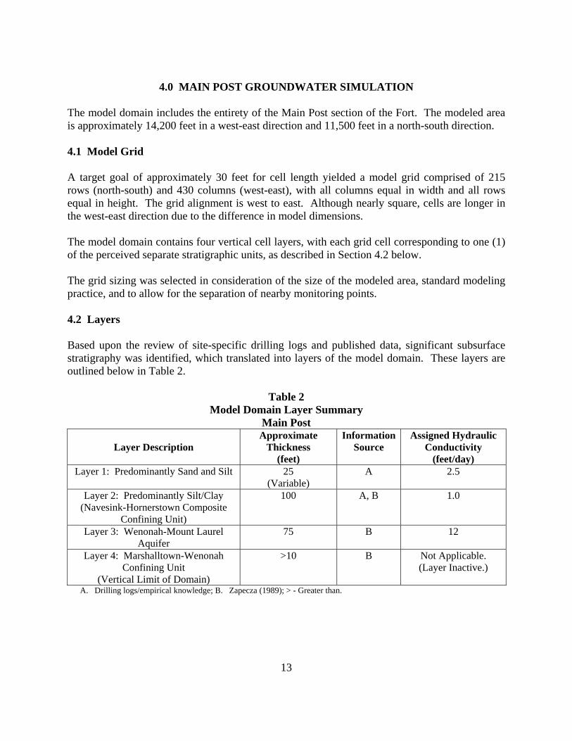
The model domain includes the entirety of the Main Post section of the Fort. The modeled area is approximately 14,200 feet in a west-east direction and 11,500 feet in a north-south direction. 4.1 Model Grid A target goal of approximately 30 feet for cell length yielded a model grid comprised of 215 rows (north-south) and 430 columns (west-east), with all columns equal in width and all rows equal in height. The grid alignment is west to east. Although nearly square, cells are longer in the west-east direction due to the difference in model dimensions. The model domain contains four vertical cell layers, with each grid cell corresponding to one (1) of the perceived separate stratigraphic units, as described in Section 4.2 below. The grid sizing was selected in consideration of the size of the modeled area, standard modeling practice, and to allow for the separation of nearby monitoring points. 4.2 Layers Based upon the review of site-specific drilling logs and published data, significant subsurface stratigraphy was identified, which translated into layers of the model domain. These layers are outlined below in Table 2.

Table 2 Model Domain Layer Summary

Main Post

Layer Description Approximate

Thickness (feet)

InformationSource

Assigned Hydraulic Conductivity

(feet/day) Layer 1: Predominantly Sand and Silt

25

(Variable) A 2.5

Layer 2: Predominantly Silt/Clay (Navesink-Hornerstown Composite

Confining Unit)

100 A, B 1.0

Layer 3: Wenonah-Mount Laurel Aquifer

75 B 12

Layer 4: Marshalltown-Wenonah Confining Unit

(Vertical Limit of Domain)

>10 B Not Applicable. (Layer Inactive.)

A. Drilling logs/empirical knowledge; B. Zapecza (1989); > - Greater than.

14

4.3 Hydraulic Conductivity Through the course of various contaminant investigations, aquifer testing was performed consisting primarily of rising head slug tests. Hydraulic conductivity values generated from these tests were compiled and evaluated and values were selected to represent each layer in the model domain. A summary of these values is provided above in Table 2. The model domain is considered to be isotropic in the horizontal plane, with hydraulic conductivity in the north-south direction, the same as the west-east direction. Vertical hydraulic conductivity values are set to one-tenth (0.1) the horizontal value as per standard industry practice. 4.4 Storage The storage property consists of Specific Storage (Ss), Specific Yield (Sy), Total Porosity, and Effective Porosity. These parameters are discussed below. Ss is defined as the volume of water that a unit volume of aquifer releases from storage under a unit decline in hydraulic head due to aquifer compaction and water expansion. This value is not used in steady state simulations. Sy is known as the storage term for an unconfined aquifer. It is defined as the volume of water that an unconfined aquifer releases from the storage per unit surface area per unit decline in the water table. For sand and gravel aquifers, Sy is generally equal to the porosity. A typical range for Sy is 0.01 to 0.30. For the purposes of this simulation, a value of 0.2 was applied. Total Porosity is the percentage of the soil that is void of material and Effective Porosity is considered the subset of the pore space through which flow actually occurs. In most cases, these values are similar for sediments and values of 0.3 and 0.15 were deemed appropriate for Total Porosity and Effective Porosity, respectively. 4.5 Boundary Conditions Boundary conditions are used within MODFLOW to represent the system’s relationship with the surrounding systems and, in this case, describe the exchange of water between the model and the external system. They are essentially used to simulate sources and sinks for water entering and leaving the model domain.

4.5.1 Constant Head Constant Head boundary conditions are used to fix the head value in selected grid cells regardless of the system conditions in the surrounding grid cells, thereby acting as an infinite source of water entering the system or as an infinite sink for water leaving the system.

15

Constant Head boundary conditions were utilized as follows in the model domain: For Layer 1, constant head boundaries were utilized to simulate water coming into the system in shallow groundwater flow from the adjoining areas. Elevation values were assigned based upon the review of topographic data and field observations of depth to water and calculated groundwater elevations and adjusted during model calibration where needed. A constant head boundary was utilized as a sink for Layer 1 to represent the larger portions of the Shrewsbury River tributaries (Parkers Creek and Oceanport Creek). Based upon the review of Shrewsbury River stage elevation data from the USGS and site-specific data from a preliminary tidal evaluation, an elevation of two-point-five (2.5) feet above MSL was selected as a representative value for the purposes of the simulation. A smaller constant head boundary was used to simulate Husky Brook Pond. The elevation of the pond was set at six-point-five (6.5) feet above MSL as determined by the surveyed elevation of the spillway. Based upon historic aerial photograph reviews, Husky Brook Pond was constructed in the 1960's by damming the brook. For Layer 3 (Wenonah-Mt. Laurel Aquifer), a constant head boundary was used to simulate flow into the system from the western edge of the model domain. A similar constant head of lower elevation was used as a sink for this layer at the eastern edge of the model domain. Head values were estimated based upon literature values and adjusted during model calibration where needed. Head values of 30 feet (west) to 25 feet (east) above MSL were used in the simulation.

4.5.2 River Boundary

Parkers Creek The western portion of Parkers Creek is a narrow tidal creek with several tributaries. In the Main Post area, there are no spillways or other control structures. The river boundary was used to simulate the interaction between the groundwater and these stream segments. The stream elevation at the western (upstream) end of the model domain was estimated based upon land surface topography and depth to water measurements and calculated groundwater elevations. The eastern end (downstream) was set to match the elevation of the adjoining constant head boundary representing the larger open water sections of the Shrewsbury River tributaries. Husky Brook/Oceanport Creek Husky Brook is a nontidal stream which drains into Husky Brook Pond. The river boundary was used to simulate the interaction between the groundwater and the stream segment. The stream elevation at the western (upstream) end of the model domain was estimated based upon land surface topography and depth to water measurements and calculated groundwater elevations. The eastern end (downstream) was set to match the known elevation of the adjoining Husky Brook Pond.

16

Water flowing out of Husky Brook Pond over the spillway (an approximate six-point-five [6.5] elevation) drains via an underground pipe into Oceanport Creek, the western end of which is a narrow tidal creek adjoining the constant head boundary, representing the larger open water sections of the Shrewsbury River tributaries. Both the underground pipe and tidal creek are simulated via the river boundary. Parameter adjustments were made to account for the limited permeability of the pipe segment.

4.5.3 Recharge The potential for precipitation to infiltrate and replenish groundwater is affected by numerous factors, the most significant of which are typically runoff over impermeable surfaces and evapotranspiration from vegetated areas. Climatological data maintained by the New Jersey Department of Environmental Proteciton (NJDEP) suggest that the total annual precipitation for the area of the Fort is approximately 47 inches. It is estimated that more than 90 percent of precipitation never reaches groundwater due to the developed nature of the area and relatively impervious soils even in landscaped and field areas. It has been observed by Fort personnel that rainfall often causes ponding in such areas and that the ponding may persist for several days following significant rainfall events. As a percentage of average rainfall for the area, six (6) inches per year were initially used to simulate recharge. During model calibration, a recharge value of four (4) inches per year was selected to represent site conditions. This is within the range of recharge values reported in USGS documentation (Voronin, 2003) which suggests that recharge may be as high as 17 inches per year to the south of the Fort or as little as eight-tenths (0.8) of an inch per year to the north.

4.5.4 Pumping Wells A groundwater extraction recovery well at Building 699 (FTMM-53) is the only known pumping well for the Main Post area. Depth to water measurements used in the calibration of the flow model were taken with the remediation treatment system off line. Therefore, the model presented is based on nonpumping conditions. As this groundwater extraction well was installed during the remediation process, it would not have affected the historic migration of contaminants from the Building 699 area. It is anticipated that the effect of pumping would be considered for the proposed site-specific evaluation of that area.

17

5.0 MAIN POST MODEL RESULTS

The groundwater flow model simulation was performed under steady state conditions using the WHS Solver for Visual MODFLOW, a proprietary solver developed by Waterloo Hydrogeologic Inc. of Ontario, Canada. 5.1 Model Calibration The goal for calibration is to identify values for hydrologic properties that provide a reasonable fit between the simulated water levels and those measured at the site and the corresponding groundwater flow direction indicated (perpendicular to lines of equal head). The suggested groundwater flow directions indicated by the groundwater flow model are generally consistent with that seen in previous groundwater investigations, and are also favorable when compared to groundwater contour maps prepared using field depth to water measurements collected on January 28, 2010. Groundwater contour maps for the January 2010 measurements are presented for comparison in Appendix VIII. In general, groundwater flow is from areas of relatively high topographic elevations toward lower topographic elevations where the site's surface water features are located. The simulation shows that the central portion of the Main Post is a relative high (groundwater divide) being that this portion of the Fort is almost completely surrounded by low elevation surface water. It was observed during model calibration that calculated heads for monitoring wells in this central portion (i.e., Buildings 699 and 750) tended to be less than the corresponding observed heads. Furthermore, it was observed that changes to the model calibration which raised heads in this area, such as an increase in recharge, tended to exacerbate conditions in other portions of the model where measured heads tended to be above their measured counterparts. To select the best overall fit to the field data set, a comparison was performed which evaluated the combination of the following key parameters:

Open Water River Elevation – This is the average elevation for the open water areas of the Shrewsbury River tributaries. Based upon the tidal study data, values of 1.5 feet above MSL and 2.5 feet above MSL were selected.

Horizontal Hydraulic Conductivity – Average values for horizontal hydraulic

conductivity (Horizontal K) of 1.0 feet/day, 1.75 feet/day, and 2.5 feet/day were selected for comparison. Vertical conductivities remained at one-tenth the horizontal value.

Groundwater Recharge from Precipitation – Average values for groundwater recharge

from precipitation of 1, 2, 3, and 4 inches/year were selected.

18

The resulting matrix of calibration statistics from the 24 simulation runs is provided below in Table 3. A description of the calibration statistics follows Table 3.

Table 3

Calibration Statistics Summary Main Post

River Stage @ 2.5 Feet, Horizontal K=1 Recharge (Inches)

Absolute Residual Mean (Feet)

Normalized Root Mean Squared (%)

Correlation Coefficient

4 2.45 18.196 0.786 (3) 3 2.249 16.317 0.779 2 2.128 15.210 0.769 1 2.084 15.055 0.754

River Stage @ 2.5 Feet, Horizontal K=1.75 Recharge (Inches)




4 2.138 15.440 0.784 3 2.056 14.688 0.777 2 2.029 14.615 0.768 1 2.082 15.253 0.753





4 2.033 14.598 0.779 3 2.009 14.441 0.772 2 2.032 14.825 0.763 1 2.122 15.724 0.749

19

Table 3

(Continued) Calibration Statistics Summary

Main Post River Stage @ 1.5 Feet, Horizontal K=1

Recharge (Inches)




4 2.281 17.064 0.787 (2) 3 2.093 15.387 0.78 2 1.995 14.607 0.771 1 2.007 14.902 0.757





4 1.976 14.537 0.788 (1) 3 1.929 (2) 14.139 (2) 0.782 2 1.956 14.494 0.773 1 2.064 15.562 0.761





4 1.922 (1) 14.061 (1) 0.785 3 1.94 (3) 14.289 (3) 0.779 2 2.005 15.080 0.771 1 2.149 16.363 0.759

The three (3) most favorable values in each category are marked as shown. Calibration statistics are produced by MODFLOW by analyzing the difference between the calculated heads and the observed results. The difference between calculated and observed values is also known as the Residual. Absolute Residual Mean – The Absolute Residual Mean measures the average magnitude of the Residuals. A smaller Absolute Residual Mean indicates a better fit between the calculated and observed values. Normalized Root Mean Squared –Normalized Root Mean Squared is expressed as a percentage and accounts for the scale of the potential range of data values. Smaller percentage values indicate a better fit between the calculated and observed values.

20

Correlation Coefficient – Correlation Coefficients range in value from - 1.0 to 1.0. This parameter determines whether two (2) ranges of data move together. For example, values closer to 1.0 indicate that large values of one (1) data set are associated with large values of the other data set (positive correlation). A Correlation Coefficient of 1.0 would indicate a perfect fit of the data. Based upon the review of the calibration statistics summary above, the combination of River Stage Elevation at one-point-five (1.5) feet above MSL, Horizontal Conductivity at two-point-five (2.5) feet/day, and Recharge of four (4) inches/year, was selected as the best overall fit. Piezometric heads for Layers 1 through 3 of the groundwater flow model and supporting documents describing the model output and calibration statistics are included in Appendix IX. 5.2 Groundwater Flow Conditions Summary In general, the Main Post area can be characterized as having a small hydraulic gradient. When combined with the low hydraulic conductivity of the aquifer materials, this translates into very slow groundwater migration. Particle markers, which represent typical travel paths and speeds for water molecules in the system, indicate extremely long travel times. In several areas of the Main Post, representative markers did not reach the nearest surface water "sink" within the 200-year travel time shown. As a result of the slow groundwater velocity, recharge to the aquifer from rainfall (although very limited) has the effect of adding a downward component to the groundwater flow. When applied to the understanding of contaminated areas, the net result of these physical conditions would likely be groundwater contaminant plumes without a dominant elongation in a downgradient direction and vertical contaminant migration would typically be heavily retarded by the fine-grained aquifer materials present at depth.

21

6.0 CHARLES WOOD AREA GROUNDWATER SIMULATION The model domain includes the entire Charles Wood area of the Fort. The modeled area is approximately 8,950 feet in a west-east direction and 7,900 feet in the north-south direction. 6.1 Model Grid A target goal of approximately 30 feet for cell length yielded a model grid comprised of 280 rows (north-south) and 280 columns (west-east), with all columns equal in width and all rows equal in height. The grid alignment is west to east. Although nearly square, cells are longer in the west-east direction due to the difference in model dimensions. The model domain contains five (5) vertical cell layers. Layers 1, 3, and 4 correspond to one (1) of the perceived separate stratigraphic units, as described below in Section 7.2. The second stratigraphic unit is divided into two (2) cell layers to resolve a MODFLOW run conflict (probable dry cell) related to the thin overlying surface layer in the southern portion of the model domain. The grid sizing was selected in consideration of the size of the modeled area, standard modeling practice, and to allow for separation of nearby monitoring points. 6.2 Layers Based upon the review of site-specific drilling logs and published data, significant subsurface stratigraphy was identified, which translated into layers of the model domain. These layers are outlined below in Table 4.

Table 4 Model Domain Layer Summary

Charles Wood Area

Layer Description Approximate

Thickness (Feet)

Information Source

Assigned Hydraulic Conductivity

(Feet/Day) Layer 1: Predominantly Sand and Silt

20 (Variable) A 5.0

Layer 2: Predominantly Silt/Clay (Navesink - Hornerstown

Composite Confining Unit) (Note: Occupies Two [2] Grid Layers.)

100 A, B 1.0

Layer 3: Wenonah - Mount Laurel Aquifer

75 B 12

Layer 4: Marshalltown-Wenonah Confining Unit

(Vertical Limit of Domain.)

>10 B Not Applicable. (Layer Inactive.)

A. Drilling logs/empirical knowledge; B. Zapecza (1989); > - Greater than.

22

6.3 Hydraulic Conductivity Through the course of various contaminant investigations, aquifer testing was performed consisting primarily of rising head slug tests. Hydraulic conductivity values generated from these tests were compiled and evaluated and values were selected to represent each layer in the model domain. A summary of these values is provided above in Table 3. The model domain is considered to be isotropic in the horizontal plane, with hydraulic conductivity in the north-south direction, the same as the west-east direction. Vertical hydraulic conductivity values are set to one-tenth (0.1) the horizontal value as per standard industry practice. 6.4 Storage The storage property consists of Specific Storage (Ss), Specific Yield (Sy), Total Porosity, and Effective Porosity. These parameters are discussed below. Ss is defined as the volume of water that a unit volume of aquifer releases from storage under a unit decline in hydraulic head due to aquifer compaction and water expansion. This value is not used in Steady State simulations. Sy is known as the storage term for an unconfined aquifer. It is defined as the volume of water that an unconfined aquifer releases from storage per unit surface area per unit decline in the water table. For sand and gravel aquifers, Sy is generally equal to the porosity. A typical range for Sy is 0.01 to 0.30. For the purposes of this simulation, a value of 0.2 was applied. Total Porosity is the percentage of the soil that is void of material and Effective Porosity is considered the subset of the pore space through which flow actually occurs. In most cases, these values are similar for sediments and values of 0.3 and 0.15 were deemed appropriate for total porosity and effective porosity, respectively. 6.5 Boundary Conditions Boundary Conditions are used within MODFLOW to represent the system’s relationship with the surrounding systems and, in this case, describe the exchange of water between the model and the external system. They are essentially used to simulate sources and sinks for water entering and leaving the model domain.

6.5.1 Constant Head Constant Head boundary conditions are used to fix the head value in selected grid cells regardless of the system conditions in the surrounding grid cells, thereby acting as an infinite source of water entering the system or as an infinite sink for water leaving the system.

23

Constant Head boundary conditions were utilized as follows in the model domain: For Layer 1, constant head boundaries were utilized to simulate water coming into the system in shallow groundwater flow from the adjoining areas. Elevation values were assigned based on the review of topographic data and field observations of depth to water and calculated groundwater elevations and adjusted during model calibration where needed. A constant head boundary was also utilized as a sink for Layer 1 to represent Wampum Lake. The elevation of the pond was set to 18 feet above MSL based upon the review of topographic data for the area. For Layer 3 (Wenonah-Mt. Laurel Aquifer), a constant head boundary was used to simulate flow into the system from the western edge of the model domain. A similar constant head of lower elevation was used as a sink for this layer at the eastern edge of the model domain. Head values were estimated based upon literature values and adjusted during model calibration where needed. Head values of 60 feet (west) to 50 feet (east) above MSL were used in the simulation.

6.5.2 River Boundary Due to the position of Charles Wood area topographically upgradient from the Main Post, the streams described below represent upstream portions of those same watercourses. Parkers Creek Branch The western portion of Parkers Creek Branch is a nontidal stream with small unnamed tributaries. In the Charles Wood area, there are no spillways or other control structures. The river boundary was used to simulate the interaction between the groundwater and these stream segments. The stream elevations at both the western (upstream) and eastern (downstream) ends of the model domain were estimated based upon land surface topography and depth to water measurements and calculated groundwater elevations for nearby monitoring wells. Wampum Brook Wampum Brook is a nontidal stream which drains into Wampum Pond. There are two (2) sections to Wampum Brook: a northern branch which is centrally located within the Charles Wood area and a southern branch, which is located toward the southern end of the area. In the Charles Wood area, there are no spillways or other control structures. The river boundary was used to simulate the interaction between the groundwater and the stream segments. The stream elevations at the western (upstream) ends of the model domain were estimated based upon land surface topography and depth to water measurements and calculated groundwater elevations for nearby monitoring wells. The eastern end (downstream) was set to match the assigned elevation of the adjoining Wampum Pond.

24

6.5.3 Recharge

The potential for precipitation to infiltrate and replenish groundwater is affected by numerous factors, the most significant being runoff over impermeable surfaces and evapotranspiration from vegetated areas. Climatological data maintained by the NJDEP suggest that total annual precipitation for the area of the Fort is approximately 47 inches. It is estimated that more than 90 percent of precipitation never reaches groundwater due to the developed nature of the area and relatively impervious soils even in landscaped and field areas. It has been observed by Fort personnel that rainfall often causes ponding in such areas and that the ponding may persist for several days following significant rainfall events. As a percentage of average rainfall for the area, six (6) inches per year was initially used to simulate recharge. During model calibration, a recharge value of four (4) inches per year was selected to represent site conditions. This is within the range of recharge values reported in USGS documentation (Voronin, 2003) which suggests that recharge may be as high as 17 inches per year to the south of the Fort or as little as eight-tenths (0.8) of an inch per year to the north.

6.5.4 Pumping Wells There are several pumping wells known for the Charles Wood area. A groundwater remediation recovery well is present at Building 2700 (CW-1, FTMM-22) and a series of five (5) irrigation wells are located within the golf course in the northeastern portion of the area. Depth to water measurements used in the calibration of the flow model were taken with the Building 2700 recovery well off line. Furthermore, the irrigation wells were not operating during the winter months when the depth to water measurements were collected. Therefore, the model presented is based upon nonpumping conditions. As the recovery well was installed during the remediation process, it would not have affected the historic migration of contaminants from the Building 2700 area. The irrigation wells have operated on a seasonal basis for many years. It is anticipated that the effect of pumping would be considered for the proposed site-specific evaluation of that area.

25

7.0 CHARLES WOOD AREA MODEL RESULTS

The groundwater flow model simulation was performed under steady state conditions using the WHS Solver for Visual MODFLOW, a proprietary solver developed by Waterloo Hydrogeologic Inc. of Ontario, Canada. 7.1 Model Calibration The goal for calibration is to identify values for hydrologic properties that provide a reasonable fit between simulated water levels and those measured at the site and the corresponding groundwater flow direction indicated (perpendicular to lines of equal head). The suggested groundwater flow directions indicated by the groundwater flow model are generally consistent with that seen in previous groundwater investigations and are also favorable when compared to groundwater contour maps prepared using field depth to water measurements collected in December of 2009. Groundwater contour maps for the December 2009 measurements are presented for comparison in Appendix X. In general, groundwater flow is from areas of relatively high topographic elevations toward lower topographic elevations where site surface water features are present. It was observed during model calibration that calculated heads for monitoring wells in the western portion of the site, such as the CW-1 (FTMM-22) and CW-3 (FTMM-25) areas, tended to be less than the corresponding observed heads, while sites in the central portion of the model area (Building 2567 [FTMM-58] and CW-6 [FTMM-28] Area) tended to be above their measured counterparts. A summary of calibration statistics for the Charles Wood area model is provided below in Table 5.

Table 5 Calibration Statistics Summary

Charles Wood Area Recharge @ 4 Inches/Year, Horizontal K=5.0 Feet/Day

Absolute Residual Mean (Feet) 1.083

Normalized Root Mean Squared (%) 4.121

Correlation Coefficient 0.994

Piezometric heads for Layers 1 through 3 of the groundwater flow model and supporting documents describing the model output and calibration statistics are included in Appendix XI.

26

7.2 Groundwater Flow Conditions Summary When compared to the Main Post area, the Charles Wood Area is characterized as having a moderate hydraulic gradient and corresponding groundwater migration velocities. Groundwater flow tends to be predominantly horizontal toward the streams which traverse the parcel. Particle markers, which represent typical travel paths and speeds for water molecules in the system, tended to reach the nearest surface water sink within 10 to 20 years, in contrast to the Main Post area, with travel times in excess of 200 years. Due to the faster groundwater velocities, varying the recharge to the aquifer from rainfall has a limited effect on groundwater flow direction. When applied to the understanding of contaminated areas, the net result of these physical conditions would likely be groundwater contaminant plumes with a dominant elongation in a downgradient direction. Vertical contaminant migration would typically be retarded by the fine-grained aquifer materials present at depth.

27

8.0 REFERENCES

Jablonski, L.A., 1968, Groundwater Resources of Monmouth County, New Jersey. USGS Special Report 23, USGS, Washington, DC Martin, M., 1998, Groundwater Flow in the New Jersey Coastal Plain. USGS Professional Paper 1404-H Minard, J.P., 1969, Geology of Sandy Hook Quadrangle in Monmouth County, New Jersey. U.S. Government Printing Office, Washington, DC New Jersey Geologic Survey, 1994, Geologic Map of New Jersey USDA Soil Conservation Service, 1989, Soil Survey of Monmouth County, New Jersey

USGS, 1981, Long Branch Quadrangle Map

Voronin, Lois M., 2003 USGS, Water-Resource Investigations Report 03-4268, Documentation of Revisions to the Regional Aquifer System Analysis Model of the New Jersey Coastal Plain VERSAR, Inc., October 2003, Remedial Investigation Report for the M-18 Landfill Site, Fort Monmouth, New Jersey Weston (Roy F. Weston, Inc.), December 1995, Site Investigation Report - Main Post and Charles Wood Areas, Fort Monmouth, New Jersey Zapecza, O., 1989, Hydrogeologic Framework of the New Jersey Coastal Plain, U.S.Geological Survey Professional Paper 1404-B. U.S. Government Printing Office, Washington, DC

modflow groundwater modeling us army, fort … · modflow groundwater modeling us army, fort...

Documents