modified genetic algorithm for simple straight and u-shaped assembly line balancing with fuzzy...

1 23

Journal of Intelligent Manufacturing ISSN 0956-5515 J Intell ManufDOI 10.1007/s10845-014-0978-4

Modified genetic algorithm for simplestraight and U-shaped assembly linebalancing with fuzzy processing times

M. H. Alavidoost, M. H. Fazel Zarandi,Mosahar Tarimoradi & Yaser Nemati

1 23

Your article is protected by copyright and all

rights are held exclusively by Springer Science

+Business Media New York. This e-offprint is

for personal use only and shall not be self-

archived in electronic repositories. If you wish

to self-archive your article, please use the

accepted manuscript version for posting on

your own website. You may further deposit

the accepted manuscript version in any

repository, provided it is only made publicly

available 12 months after official publication

or later and provided acknowledgement is

given to the original source of publication

and a link is inserted to the published article

on Springer's website. The link must be

accompanied by the following text: "The final

publication is available at link.springer.com”.

J Intell ManufDOI 10.1007/s10845-014-0978-4

Modified genetic algorithm for simple straight and U-shapedassembly line balancing with fuzzy processing times

M. H. Alavidoost · M. H. Fazel Zarandi ·Mosahar Tarimoradi · Yaser Nemati

Received: 10 January 2014 / Accepted: 3 October 2014© Springer Science+Business Media New York 2014

Abstract This paper aims at the straight and U-shapedassembly line balancing. Due to the uncertainty, variabilityand imprecision in actual production systems, the processingtime of tasks are presented in triangular fuzzy numbers. Inthis case, it is intended to optimize the efficiency and idle-ness percentage of the assembly line as well as and con-currently with minimizing the number of workstations. Tosolve the problem, a modified genetic algorithm is proposed.One-fifth success rule in selection operator to improve thegenetic algorithm performance. This leads genetic algorithmbeing controlled in convergence and diversity simultaneouslyby the means of controlling the selective pressure. Also afuzzy controller in selective pressure employed for one-fifthsuccess rule better implementation in genetic algorithm. Inaddition, Taguchi design of experiments used for parame-ter control and calibration. Finally, numerical examples arepresented to compare the performance of proposed methodwith existing ones. Results show the high performance of theproposed algorithm.

Keywords Assembly line balancing · Genetic algorithm ·One-fifth success rule · Fuzzy numbers · Taguchi method

M. H. Alavidoost (B) · M. H. F. Zarandi · M. TarimoradiDepartment of Industrial Engineering, Amirkabir Universityof Technology, P.O. Box 15875-4413, Tehran, Irane-mail: [email protected]

M. H. F. Zarandie-mail: [email protected]

M. Tarimoradie-mail: [email protected]

Y. NematiDepartment of Industrial Engineering, University of Tehran,Tehran, Irane-mail: [email protected]

Introduction

The competitive market leads producers to promote theirmanufacturing systems by more efficient and effective plan ina short period of time. So, in actual design of a manufacturingsystem, programming an efficient assembly line continuouslywas an important and controversial issue in the past decades(Baudin 2002). The manufacturing assembly line for the firsttime introduced by Henry Ford in the early 1900s (Fonsecaet al. 2005). The assembly line balancing problem (ALBP)involves assigning needed tasks for producing a product asseries or batches to a set of workstations, so that objectivefunctions being optimized subject to limitations (Boysen etal. 2007). From this point of view, tasks sequence is the mostimportant issue that should be considered in an assembly linedevelopment (Kao 1976).

There are numerous reviews about ALBP in the litera-ture (Boysen et al. 2007; Battaïa and Dolgui 2013; Baybars1986b; Becker and Scholl 2006; Ghosh and Gagnon 1989;Scholl 1999; Scholl and Becker 2006; Tasan and Tunali2008), and classified it generally into two main types ofSimple ALBP (SALBP) and Generalized ALBP (GALBP).GALBP versions have the extra features such as cost goals,station parallelization, mixed-model production, etc. in com-parison with SALBPs (Becker and Scholl 2006). SALBPversions from goal point of view presented in Table 1.

SALBP-F is a feasibility problem for a given combi-nation of time cycle and workstations number. SALBP-1andSALBP-2 are dual of each other, because the SALBP-1goal is minimizing the workstation number for a given cycletime, while the SALBP-2 goal is minimizing the cycle timefor a given workstations number. In SALBP-E cycle timeand workstations number ought to be minimized simultane-ously so that efficiency can be maximized. In addition to thepresented classification, assembly lines can be divided into

123

Author's personal copy

J Intell Manuf

Table 1 Versions of SALBP (Scholl and Becker 2006)

No. of workstation Cycle time

Given Minimize

Given SALBP-F SALBP-2

Minimize SALBP-1 SALBP-E

two categories, respecting to their layout, Straight Assem-bly Lines and U-Shaped Assembly Lines. Straight assemblyline considered as one of the most important traditional massproduction sections, and then U-shaped assembly lines wasdefined to reduce the costs and improve Just-In-Time (JIT)(Monden 1983). On the other hand, it can be divided intosingle models and mixed models respecting to their types ofproducts (Boysen et al. 2007). In the single model of assem-bly line, only one product can be produced in manufacturingline, and others that can produce more than one product,called mixed model assembly lines.

SALB problem is a single model for straight assem-bly line balancing and U-shape layout SALB called SimpleU-line balancing (SULB).

The ALBPs were proven to be NP-hard by Gutjahr andNemhauser (1964) and Ajenblit and Wainwright (1998).Therefore, according to the difficulty of such problems,lots of efforts exploited to development and expansion ofheuristic methods such as the ranked positional weightingtechnique (RPWT) (Helgeson and Birnie 1961), COMSOALtechnique (Arcus 1966), MALB technique (Dar-El 1973),MUST technique (Dar-El and Rubinovitch 1979, and LBHAmethod (Baybars 1986a), A critical path method (CPM)based approach (Avikal et al. 2013), and also meta-heuristicmethods such as genetic algorithm (GA) (Ajenblit andWainwright 1998; Falkenauer and Delchambre 1992), sim-ulated annealing (SA) (Baykasoglu 2006), Tabu search (TS)(Peterson 1993; Lapierre et al. 2006), Particle swarm opti-mization (PSO) (Jian-sha et al. 2009), and ant colony opti-mization (ACO) (Sabuncuoglu et al. 2009).

A multi-objective GA for solving U-shaped AssemblyLine problem proposed by Hwang et al. (2008), and theydid a comparison between Straight and U-shaped AssemblyLines. Kim et al. (2009) rendered a mathematical model andGA for A two-sided assembly line. In Hwang and Katayama(2009) work a multi-decision genetic approach for solvingmixed-model U-shaped lines have been proposed which val-idated through a case study. A TS algorithm for solving two-sided assembly line problem prepared by Özcan and Toklu(2009) and the results benchmarked by existed approaches.An adaptive GA for solving ALBP offered by Yu and Yin(2010) which they proofed their algorithm efficiency withan example. In another noteworthy work a hybrid GA pro-posed by Akpınar and Mirac Bayhan (2011) and deployedfor solving ALB mixed model with parallel workstation and

zoning constraints. Zhang and Gen (2011) used a multi-objective GA to solve mixed-model assembly lines. Kazemiet al. (2011) proposed a two-stage GA for solving mixed-model U-shaped assembly lines. Nearchou (2011) used novelmethod based on PSO for SALBP and compared it with exist-ing method. Rabbani et al. (2012) proposed a heuristic algo-rithm based on GA for mixed-model two-sided assembly line.Chang et al. (2012) focused on productivity in printed circuitboard assembly line and rendered a GA with External Self-evolving Multiple Archives solving this problem. Chutimaand Chimklai (2012) used a PSO to solve multi-objectivetwo-sided mixed-model assembly line and showed if theirproposed algorithm be combined with local search schemequality of its solution set would be better. In another work,Purnomo et al. (2013) offered a mathematical model for two-sided assembly line and solved it with GA and iterative first-fit rule method, and lastly compared result of these meth-ods. Manavizadeh et al. (2013) proposed a SA for a mixedmodel assembly U-line balancing type-I problem and com-pared algorithm results with exact method. Yuan et al. (2013)proposed an integer programming modeland a new meta-heuristic for mixed-model assembly line problem. Hamza-dayi and Yildiz (2013) used a SA algorithm for problemsline balancing and model sequencing in U-shaped assemblylines. Dou et al. (2013) proposed a discrete PSO for solv-ing SALBP-1 and compared their results with GA. Kalayciand Gupta (2013) used a PSO with a neighborhood-basedmutation operator for solving sequence-dependent disassem-bly line balancing. Li et al. (2014) created a mathematicalmodel and a novel multi-objective optimization algorithm tosolvetwo-sided assembly line. Delice et al. (2014) proposed amodified PSO for two-sided assembly line problem. Zha andYu (2014) proposed a hybrid ant colony algorithm for solv-ing U-line balancing and rebalancing problem and comparedtheir algorithm results with existing methods. Al-Zuheri etal. (2014) considered mixed-model assembly line and useda GA to solve it.

Among these meta-heuristic methods, most of studieswere devoted to GA and these previous research has indi-cated that there must be sufficient motivation to use this pop-ular algorithm for solving emerged and defined problem. Toperform a controlled random search for identifying the opti-mal solution, an alternative traditional optimal technique inthe complex circumstances was provided (Tasan and Tunali2008).

Concentration of many researchers on GA and its popu-larity was author motivation to improve the performance ofthis meta-heuristic through a modification as a part of con-tribution of this paper and put it into practice to solve thementioned controversial problem.

Numerous works reviewed which solved ALBPs in crispcircumstance whilst actual world problems usually deal withuncertainty and vagueness. To represent uncertainty, fuzzy

123


J Intell Manuf

numbers can reflect the ambiguity of real data well. Thereis a considerable attention in the ALBPs literature that onlysome of them managed to solve such problems in fuzzy envi-ronment. In other words, in comparison with crisp ALBPs,a few numbers of researchers focused on fuzzy ALBP so far(Scholl and Becker 2006; Tasan and Tunali 2008). Betweenthe articles used in solving fuzzy ALBP by précised methods,researches (Toklu and özcan 2008; Kara et al. 2009; Zhangand Cheng 2010; La Scalia 2013) are noticeable.

Through the studies in this area, ones that use heuristicand meta-heuristic methods for solving the ALBP in fuzzyenvironment are rare. In the 90s Tsujimura et al. (1995) andGen et al. (1996) initialized using fuzzy GA for this prob-lem. With a typical GA provided that the tasks processingtime was presented in fuzzy numbers, they solved SALBP-1. While Brudaru and Valmar (2004) proposed a combinedGA with Branch and Bound method to solve SALBP-1.Fonseca et al. (2005) presented modified Ranked PositionalWeighting Technique and COMSOAL method with fuzzynumbers, and applied it to solve these sort of problems.Hop (2006) proposed a heuristic method to solve a fuzzymixed-model ALBP. Zhang et al. (2009) prepared a heuris-tic method to solve SULBP with fuzzy numbers. Özbakırand Tapkan (2010) presented a model for two-sided ALBPand solved this problem by Bees algorithm. Zacharia andNearchou (2012) also introduced a multi-objective GA tosolve SALBP-2 with fuzzy numbers, in which they appliedweighted sum of objectives. Zacharia and Nearchou (2013)presented a meta-heuristic algorithm based on genetic algo-rithm for solving SALBP-E.

As mentioned, since numerous researchers used GA andits popularity, this paper tends to improve performance ofthis algorithm through a modification. Also this is notewor-thy that no research considered and solved SULB-1 usingmeta-heuristic methods in fuzzy circumstance. So this paperconsidered the SALB-1 and SULB-1 in which a modified GApresented with the one-fifth success rule that result in enhanc-ing the performance. A fuzzy controller for better adapta-tion between GA and one-fifth success rule have renderedand also the parameters of proposed algorithm calibrated byTaguchi design of experiments. Due to the uncertainty in thereal world, fuzzy numbers have been used to represent theassembly line cycle and processing time.

The rest of the paper is organized as follows: In “Problemformulation” section, the main characteristics of SALBP andSULBP are represented. In “Fuzzy numbers arithmetic andranking” section, fuzzy arithmetic is provided as well as anumber of criteria to sort fuzzy numbers. Genetic algorithm,one-fifth success rule and also the procedure of genetic algo-rithm modification with one-fifth success rule are presentedin “Genetic algorithm” section. In “Comparison” section, atfirst the parameters of proposed algorithm would be cali-brated using Taguchi method, and after that the proposed

algorithm would be examined by benchmarks and its resultwould be compared with existing methods. Finally, conclu-sions and some guidelines for future studies are provided in“Conclusion” section.

Problem formulation

This section represents the main characteristics of SALBP-1 and SULBP-1. As mentioned before, assembly line is aseries of locations which is called workstations, and a subsetof tasks that are performed and need to be done for produc-tion of a unit in these locations (Gen et al. 1996). For theseproblems, the available information is as follows (Miltenburgand Wijngaard 1994):

• A given set of tasks J = {i |i = 1, 2, . . . n}.• The set of tasks’ needed time which is shown as T ={

ti |i = 1, 2, . . . n}.

• Each task’s allocated time that will be presented as trian-gular fuzzy number (TFN).

• The set of precedence relations P = {(a, b)|task a mustbe completed before task b}.

• Maximum allowed fuzzy cycle time(

Cmax

).

Symbols of this article are listed below:

• ti : Fuzzy processing time that is represented by TFNs.• Sk : Set of activities which done in k workstation Sk =

{i |task i is done at workstation k},∀k = 1, . . . ,m• t (Sk): Fuzzy time that every workstation needs to com-

plete all the required tasks.• c : Assembly line’s fuzzy cycle time, i.e. max

k

{t (Sk)

}.

• Cmax : Maximum allowed fuzzy cycle time.• T : Total processing time.• Ik : Fuzzy idle time for workstation Sk, (k = 1, . . . ,m).• E : Fuzzy balance efficiency.• I D Fuzzy idle percentage of assembly line.

In this problem, there are a number of workstations which arepresented by set of W S = {ws1, ws2, . . . , wsm}, and eachtask should be assigned only to one of these workstations. Inaddition, the “J” set should be allocated into workstations,so that the limits of Eqs. (1)–(3) are satisfied (Tsujimura etal. 1995; Gen et al. 1996):

m⋃

k=1

Sk = J (1)

Sk

⋂

k �=l

Sl = ∅ (2)

∑

iεSk

ti ≤ Cmax k = 1, 2, . . . ,m (3)

123


J Intell Manuf

The first and second constraints guarantee that all tasks allo-cated to the workstations and each task will be allocated onlyto one workstation. The third one ensures that each worksta-tion cycle time will not be greater than maximum allowablefuzzy cycle time. In SALB, j th work can be allocated to kthworkstation, only when its prior tasks have been assignedto 1, 2 . . . kth workstations, whilst in SULB, the j th taskcan be allocated to kth workstation, only when all its pre-decessor tasks or/and all its successor tasks have been allo-cated to 1, 2 . . . kth workstations (Miltenburg and Wijngaard1994). Thus, in tasks allocation, constraint equation (4) forSALB and constraint equation (5) for SULB should be met(Miltenburg and Wijngaard 1994).

I f (a, b) ∈ P, a ∈ Sk, b ∈ Sl , then k ≤ l, f or all a;(4)

I f (a, b) ∈ P, a ∈ Sk, b ∈ Sl , then k ≤ l, f or all a;or, I f (b, c) ∈ P, b ∈ Sk, c ∈ Sr , then r ≤ k, f or all c;

(5)

Constraint (4) is defined for SALB and ensures its com-pliance with predecessor constraints. Also constraint (5) isdefined for SULB, guaranteeing the compliance of at leastone of the predecessor or successor constraints.

Beside the main goal of SALBP-1andSULBP-1, that isminimizing the number of workstations, it’s possible todefine other goals for comparing the solutions with sameworkstation numbers. According to the problem, there arefollowing result [Eqs. (6)–(11)] (Fonseca et al. 2005; Zhanget al. 2009):

t (Sk) =∑

iεSk

ti , k = 1, . . . ,m (6)

c = maxk

{t (Sk)

}(7)

Ik = Cmax − t (Sk) , k = 1, . . . ,m (8)

T =m∑

k=1

t (Sk) (9)

E = T /(m × c) (10)

˜I D =∑m

k=1(Cmax − t (Sk))

/(m × Cmax ) (11)

Figure 1 determines the main difference between SALBand SULB. It depicts a SALB and a SULB, with the cycletime of 10 min. Each node represents a task and the numberabove, represents the processing time for each node. As seen,in the SALB, the tasks are allocated to five workstations (withefficiency of 39/50). Instead, in SULB, tasks are allocated to4 workstations (with efficiency of 39/40).

Equation (6) calculates the fuzzy cycle time of each work-station and Eq. (7) calculates the fuzzy cycle time of assemblyline. Formula (8) calculates the fuzzy idle percentage of theassembly line. By Eqs. (9) and (10), the fuzzy efficiency of

Fig. 1 Straight assembly line (a), U-Shaped assembly line (b)

X

Fig. 2 Triangular fuzzy number

assembly line and by Eq. (11) fuzzy idle percentage of theassembly line could be calculated.

Fuzzy numbers arithmetic and ranking

This section provides fuzzy arithmetic as well as a num-ber of criteria to rank fuzzy numbers. Because of vaguenessand uncertainty in the real world, data are fuzzy numbers.In this paper, as shown in Fig. 2, TFNs are used to presentthe processing time of the tasks. A TFN can be characterizedby three parameters A = (A1, A2, A3). The reason of usingtriangulated data in this paper is because of its computationalsimplicity in comparison with other fuzzy data, as its con-sidered calculations in Eqs. (12)–(15) (Kaufmann and Gupta1991):

A + B = (A1 + B1, A2 + B2, A3 + B3) (12)

A − B = (A1 − B1, A2 − B2, A3 − B3) (13)

A × B = (A1 × B1, A2 × B2, A3 × B3) (14)

A/B = (A1/B3, A2/B2, A3/B1) (15)

The operator ≤ used for comparing two fuzzy numbers informula (3) whilst for comparison and TFNs ranking fol-lowing criteria will be used for prioritization (Bortolan andDegani 1985):

123


J Intell Manuf

• Criterion 1: The data is greater which in terms of thethree points weighted average (Beginning, Peak, End) begreater [Eq. (16)]

• Criterion 2: The data is greater which in terms of themidpoint, be greater [Eq. (17)].

• Criterion 3: The data is larger so which in terms of dis-tance between the beginning and end point is greater[Eq. (18)].

F1 = A1 + 2 × A2 + A3

4(16)

F2 = A2 (17)

F3 = A3 − A1 (18)

For comparing some TFNs, initially, the criterion1[Eq. (16)] is used, If the first criterion cannot determine themajor TFN, the criterion2 [Eq. (17)] is used, and so on.

Genetic algorithm

Genetic algorithm (Holland 1975) is a popular meta-heuristicalgorithms. The majority of GAs consists of the followingsteps:

Step 1. Determine population size (nPop), maximumnumber of iteration (Itr), migration rate (α%), crossoverrate (β%), and the mutation rate (γ%), so that satisfyα + β + γ = 100 % (α is the ratio of chromosomes thatmigrate from a generation into the next. Also β and γ arethe ratio of chromosomes which are advent in each gen-eration by the crossover and mutation operations respec-tively).Step 2. Generate initial population, using random num-bers.Step 3. Calculate fitness function for each chromosome.Step 4. In case of satisfying the stopping criteria, thealgorithm stops, otherwise goes to step five.Step 5. Create the new generation, by the following meth-ods:

• Selection of α% of chromosomes from previous gen-eration (this selection is based on fitness, or random,or other methods) and placing them in the next gen-eration.

• Crossover act on the β% of the generation and placetheir children in the next generation.

• Mutation act on the γ% of the previous generationsand placing new chromosomes in the next generation(to escape from the local optimum).

Step 6. Repeat the Steps 3 and 4.

The GA’s general diagram is displayed in Fig. 3.

Yes

No

Stop

Start

Set nPop, Itr,

Initial Generation

Fitness Evaluation

Iteration > MaxItr

CrossoverMutation

Migration Population Selection

New Population

Fig. 3 General diagram of genetic algorithm (Holland 1975)

If the GA operators are defined properly and well adaptedto the problem, this algorithm would be efficient to solve theproblem. So, first of all, the algorithm operators ought to bedefined for the ALBP. To generate the initial chromosomes,permutations from one to the number of tasks will be gener-ated randomly, and to satisfy the predecessor restrictions, thegenerated chromosome should be repaired, if it’s necessary.For example, suppose that there are eight tasks that should beoptimal, in terms of sequencing. Using random numbers, apermutation would be generated from one to eight, for exam-ple [1 3 5 4 7 8 2 6], as a chromosome.

Suppose that one of the precedence relation constraints isnecessary for second task to be done before fifth task thatit makes the generated chromosome infeasible and must berepaired. To repair this chromosome, a gene containing thesecond task is to be placed before the gene containing fifthtask, and after repairing the initial chromosome it would bereordered into: [1 3 2 5 4 7 8 6].

After repairing the chromosomes, the tasks should be allo-cated to workstations. If the current workstation is k, forassigning tasks to the SALB, the task of assigning sorted tasksin chromosome to kth workstation will continue, until theworkstation’s cycle time doesn’t pass the maximum allowed

fuzzy cycle time (if the expression{∑

iεSkti + t j ≤ Cmax

}

is satisfied, then t j will be assigned into the current worksta-tion, otherwise a new workstation will be built).

Differences between the task allocations to SALB withallocation of the same task to the SULB is that in the SALBthe tasks should be selected from the beginning of the chro-mosome and be assigned to the workstations, whilst in theSULB tasks can be selected from the beginning or from the

123


J Intell Manuf

end of the chromosome. After allocating tasks to the work-stations, one has to calculate fitness function or cost for eachchromosome and then with the help of existing operators(Selection, Crossover, and Mutation) produces a new gener-ation. For “Selection” operator, Random selection, RouletteWheel selection, Tournament selection etc. can be exploited(Haupt and Haupt 2004). Also, In this paper, three methodsof Single-Point Crossover, Two-Point Crossover and Uni-form Crossover are used for “Crossover” operator (Hauptand Haupt 2004). There are different methods for the “Muta-tion” operator. In this paper, two genes and swapping themwith each other is selected randomly (Haupt and Haupt 2004).What should be noted here is that after crossover and muta-tion, the child chromosome (due to predecessor constraints)may be infeasible in this case, so the produced chromosomeshould be repaired.

One-fifth success rule

One-fifth success rule is introduced by Rechenberg (1973)for the evolutionary strategies (ES) algorithm (that is a meta-heuristic method per se) at first, that is a meta-heuristicmethod per se. Like GA, ESs use mutation and crossoverof chromosome for evolution of the generations. Each chro-mosome is presented as (x1, x2, . . . , xn, σ ) that xi s are theproblem’s variables and presented by real numbers, and σ

is the mutation step length. Rechenberg (1973) mathemati-cally had been proved one-fifth success rule for the ESs with achromosome and a child. This rule says that if the ratio of thenumber of successful mutations to number of total mutationsis equal to one-fifth, then the convergence rate to the optimumsolution will be maximum rate. For mutation in ES, severalmethods are proposed that one of them as formula (19) isadding a random normal value to all genes.

x ′i = xi + N (0, σ ) (19)

The value of σ is determined by one-fifth success rule, dur-ing the algorithm. One-fifth success rule will follow threeconditions to achieve the maximum convergence rate:

• Mode 1. If the probability of success in past k-populationswas equal to one-fifth, the mutation step length (σ ) willnot change.

• Mode 2. If the probability of success in past k-populationswas more than one-fifth, the mutation step length (σ )willincrease.

• Mode 3. If the probability of success in past k-populationswas less than one-fifth, the mutation step length (σ ) willdecrease.

In the cited modes, mode 2 used for prevent premature con-vergence by creating diversity in generations and mode 3

Fig. 4 General diagram of one-fifth rule

used for increase the speed of convergence. In fact, this algo-rithm considers diversity and convergence, simultaneously.If the diversity of chromosomes is low, to escape the localoptimum, the step length to search a wider area of the solutionspace increased here and if the convergence of chromosomesis low, for converge chromosomes to optimum solution, thesearch space narrowed by reducing the step length. The gen-eral diagram of one-fifth success rule is shown in Fig. 4 (C isa constant,β is equal to 1

past k−populations , Ps is the probabil-ity of success in past k generations, t is the iteration number,Xt presents the chromosomes in the time of t , F(Xt) is thechromosome fitness function in the time of t , σ 0 and σ are theStandard deviation from first step and next steps respectively.

Combined GA with one-fifth success rule

As mentioned before, the one-fifth success rule considersdiversity and convergence simultaneously for better search.Also in GA for simultaneous influence on diversity and con-vergence, one could use selective pressure (the probabilityof selecting the best member of the population, compared tothe average probabilities of selecting the other members ofthe population). In other words, by controlling the selectivepressure, diversity and convergence could be optimum simul-taneous. To do this, the selection operator must be definedaccording to the fitness and selective pressure that has to be

123


J Intell Manuf

entered in selective operator. In this paper, to link between fit-ness of each chromosome and its selection probability, Boltz-mann method is used Goldberg (1990), as in Eq. (20) (SP isthe Selective Pressure, fv is the fitness of vth chromosome,and Pv is the probability of selecting vth chromosome).

Pv ∝ eS P× fv (20)

According to the Eq. (20), the more fitness of the chromo-some means more probability of selection of the chromo-some. Summation of all probabilities ought to be equal toone. Thus, the probability of selecting each chromosome isdivided by the summation of probabilities (Eq. (21), N ispopulation size).

Pv = eS P× fv

∑Ni=1 eS P× fv

(21)

In order to be able to successfully enter the one-fifth successrule in probabilities, initially it should sort the existing popu-lation on the basis of chromosome fitness. Then, by increas-ing or decreasing of the SP, it has tried the ratio of totalprobability of the bottom half of the population [the WeakerHalf Probability (WHP)] be equal to one-fifth, in the otherhands invoking the one-fifth success rule tend to tune the SP[formula (22)].

W H P =N∑

v=[ N2 ]+1

Pv = 1

5(22)

SP controller

However, due to the continuous nature of the solution space,reach to the number of one-fifth is difficult (or even impos-sible). So, fuzzy terms and fuzzy rules are applied as SPcontroller in this paper. Some of used fuzzy terms defined as“Small”, “Good”, and “Big”. These fuzzy terms membershipfunctions are presented in Fig. 5.

0

0.2

0.4

0.6

0.8

1

1.2

0 0.05 0.1 0.15 0.2 0.25 0.3 0.35 0.4 0.45 0.5

Mem

bers

hip

WHP

Good Small Big

Fig. 5 Fuzzy terms membership function

If the WHP is small, the SP should be limited [For-mula (23)] otherwise it could be aroused [Formula (24)],(DoF = Degree of Firing).

IfWHPisSmall; then, S Pt+1

= S Pt ×{

1 +(

WHP − 1

5

)× DoFSmall

}(23)

IfWHPisBig; then, S Pt+1

= S Pt ×{

1 +(

WHP − 1

5

)× DoFBig

}(24)

As seem in rules (23) and (24), more distance of WHP fromone-fifth (center of good membership function) lead to moreSP variation in direction of one-fifth. Also, DoF help forlower fluctuation and SP convergent. Besides, use of momen-tum can be useful to increase the convergence celerity (For-mula (25)–(26)).

IfWHPisSmall; then, S Pt+1

= S Pt ×{

1 +(

WHP − 1

5

)× DoFSmall

}+ α (�S Pt )

(25)

IfWHPisBig; then, S Pt+1

= S Pt ×{

1 +(

WHP − 1

5

)× DoFBig

}+ α (�SPt )

(26)

α presents the momentum in formula (25)–(26). In fact, SP’svariation and direction in every iteration (�S Pt ) have aneffect on SP in the next iteration (S Pt+1) that tend to con-vergence celerity.

Defined fuzzy rules effect on SP iteratively, whilst theWHP satisfy the defined fuzzy term of good. Scilicet WHPapproximately being equal to the 1

5

(W H P ∼= 1

5

).

Comparison

In this section, first of all the parameter control mechanismwould be considered an after that the proposed modified GAwould be benchmarked with standard functions and after thatproposed algorithm examined with bench-marks of SALBP-1 and SULBP-1. And lastly comparison between proposedalgorithm and existing method would be rendered.

Problem parameters control using Taguchi method

There are various method to calibrate the meta-heuristic algo-rithm parameters that some of them are full factorial design,i.e. they examine all possible combinations (Ruiz et al. 2006;Montgomery 2008), that is intrinsically time and cost con-suming. Taguchi method (Taguchi 1986) uses special design

123


J Intell Manuf

of orthogonal arrays to study the whole parameters spacewith a small number of experiments.

Taguchi method clusters factors into two main groups:controllable and noise factors (uncontrollable). Since noisefactors are uncontrollable and their elimination is unpracticaland almost impossible, the Taguchi method tries to reach tothe best controllable factors level from robustness point ofview. In addition to determine the best factors level, Taguchiestablishes the relative importance of each factor with respectto its main impacts on the objective function (Naderi et al.2009). To analyze the experimental data and find optimalfactor combination, Taguchi method uses a criterion entitledsignal-to-noise (S/N) ratio which expected to be maximum.

Taguchi method divides objective functions into threegroups:

The smaller the better In case that approaching objectivefunction value to zero is better come in handy. In this sit-uation, S/N ratio would be calculated by formula (27), (e)determines number of experiment, Obje is objective functionvalue in eth experiment, and nExp is number of parameterscombination which should be examined.

S/N ratio = −10 log10

(∑

e

Obj2e

nExp

)

(27)

The larger the better In case that upper value of objectivefunction is better come in handy. In this situation, S/N ratiowould be calculated by formula (28).

S/N ratio = −10 log10

⎡

⎣

(Obj

2/s2

)

nExp

⎤

⎦ (28)

Nominal is best: In case that there is a specific target valuefor objective function come in handy. In this situation, S/Nratio would be calculated by formula (29).

S/Nratio = −10 log10

[∑

e

(1/Obj2

e

)

nExp

]

(29)

Controllable factors which selected for this portion are pop-ulation size, maximum number of iteration, crossover rate,and mutation rate In addition to the S/N ratio, the means asa criterion is useful for finding the best factors combination.As mentioned the S/N ratio should be maximized regardlessto the objective function type whilst for means the type ofobjective function is important and because that in assemblyline problem, most of objective functions should be mini-mized, clearly the lower means value the better. To sum up,a level for parameters should be selected which in that level,S/N ratio has maximum value and means criterion has min-imum value in comparison with the other levels, and just incase that for a level these criteria weren’t satisfied simultane-ously, another experiment for that specific parameter shouldbe design.

Proposed algorithm has been examined with three types ofbenchmarks (benchmarks were classified into three classesof A, B, and C according to their size). So, for every fac-tor according to the benchmark size three levels consid-ered which each level value caught through trial and error(Table 2).

The Minitab 17 used for Taguchi method implementation.The Taguchi experiments for each three class of A, B, and Chave done separately. S/N ratio and means criteria for A, B,and C classes exposed in Figs. 6, 7, and 8 respectively.

As clear in Fig. 6, for nPopA and γ A third level would beselected, because in comparison with other level S/N ratiohas maximum value and means has minimum value in thislevel. But for determination of ItrA and βA, extra experi-ment should be designed. The same analysis for Figs. 7 and8 comes in handy. Using exposed diagram and after com-plimentary experiments, selected levels for parameters pre-sented in Table 3.

Table 2 Parameters and theirlevels Class Parameter Symbol Level

Class A Population size nPopA nPopA(1):10, nPopA(2):20, nPopA(3):30

Maximum number of iteration ItrA ItrA(1):5, ItrA(2):10, ItrA(3):15

Crossover rate βA βA(1) : 0.7, βA (2) : 0.8, βA (3) : 0.9

Mutation rate γ A γ A(1) : 0.1, γ A (2) : 0.15, γ A (3) : 0.2

Class B Population size nPopB nPopB(1):30, nPopB(2):50, nPopB(3):70

Maximum number of iteration ItrB ItrB(1):10, ItrB(2):20, ItrB(3):30

Crossover rate βB βB(1) : 0.7, βB (2) : 0.8, βB (3) : 0.9

Mutation rate γ B γ B(1) : 0.1, γ B (2) : 0.15, γ B (3) : 0.2

Class C Population size nPopC nPopC(1):70, nPopC(2):100, nPopC(3):130

Maximum number of iteration ItrC ItrC(1):30, ItrC(2):50, ItrC(3):70

Crossover rate βC βC (1) : 0.7, βC (2) : 0.8, βC (3) : 0.9

Mutation rate γC γC (1) : 0.1, γC (2) : 0.15, γC (3) : 0.2

123


J Intell Manuf

321

140000

130000

120000

110000

100000

90000

80000

70000

60000

50000

321 321 321

nPopA

Levels of factors

Mea

n of

Mea

ns

ItrA βA γA

Main Effects Plot for MeansData Means

321

-92

-93

-94

-95

-96

-97

-98

-99

-100

-101

321 321 321

nPopA

Levels of factors

Mea

n of

SN

ratio

s

ItrA βA γA

Main Effects Plot for SN ratiosData Means

Fig. 6 Mean of means and S/N ratio for each parameter in Class A

321

70

60

50

40

30

20

321 321 321

nPopA

Levels of factors

Mea

n of

Mea

ns

ItrA βA γA


321

-30

-32

-34

-36

-38

-40321 321 321

nPopA

Levels of factors

Mea

n of

SN

ratio

s

ItrA βA γA


Fig. 7 Mean of means and S/N ratio for each parameter in Class B

80

70

60

50

40

30

20

nPopA

Levels of factors

Mea

n of

Mea

ns

ItrA βA γA


321

-30

-31

-32

-33

-34

-35

-36

-37

321 321 321

nPopA

Levels of factors

Mea

n of

SN

ratio

s

ItrA βA γA


321 321 321 321

Fig. 8 Mean of means and S/N ratio for each parameter in Class C

Table 3 Selected level of the parameters

Parameter Symbol Class A Class B Class C

Population size nPopA nPopA(3):30 nPopB(3):70 nPopC(3):130

Maximum number of iteration ItrA ItrA(1):5 ItrB(2):20 ItrC(3):70

Crossover rate βA βA(2) : 0.8 βB(1) : 0.7 βC(3) : 0.9

Mutation rate γ A γ A(3) : 0.2 γ B(1) : 0.1 γC(2) : 0.15

123


J Intell Manuf

Numerical results over evolutionary standard benchmarks

Proposed algorithm could be benchmarked rendered algo-rithms using standard functions and this also invoked forbenchmarking proposed modified GA with the listed stan-dard function in Table 4 (Molga and Smutnicki 2005).

Obviously, the proposed modified GA improves the per-formance respect to the selection operator. So, it seems thatthis is necessary to compare between selection methods intraditional GA and rendered one. There are several methodsfor selection that Roulette Wheel, Tournament, and Randomcompared with the proposed method (Table 5).

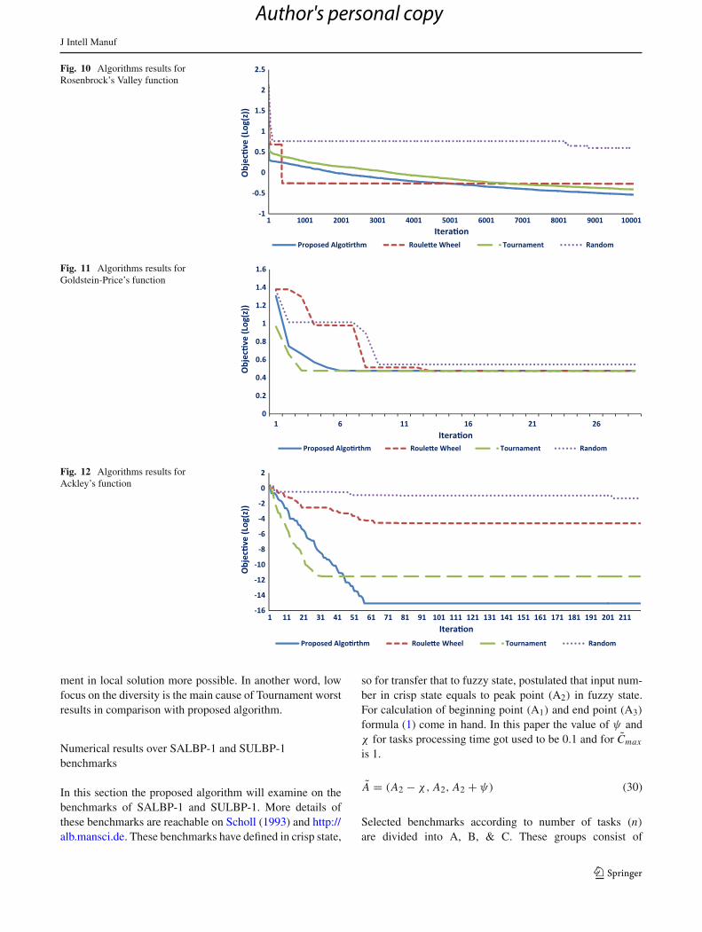
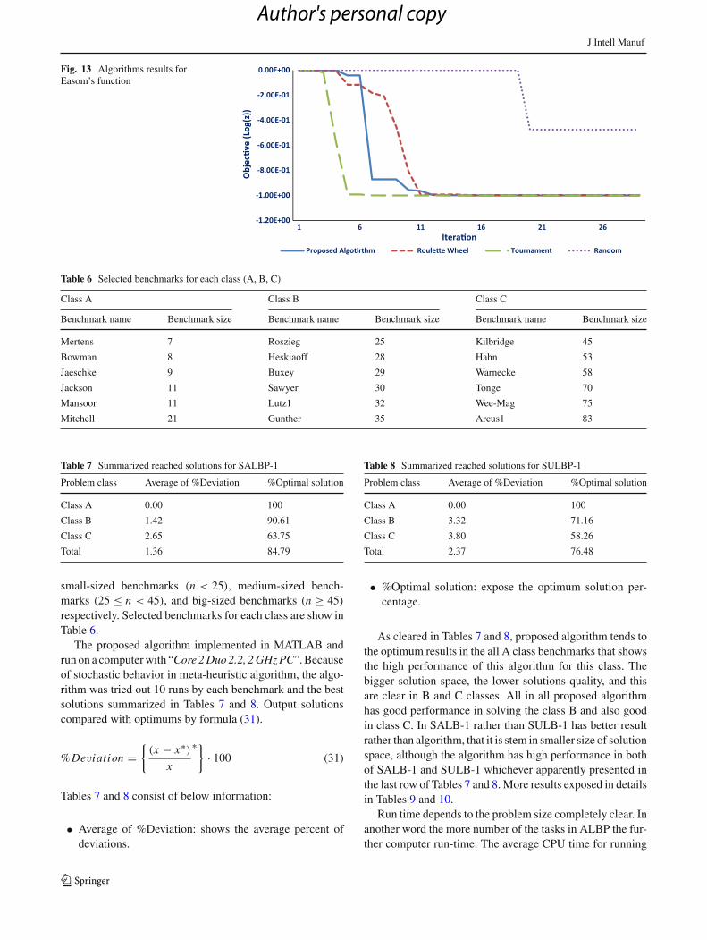
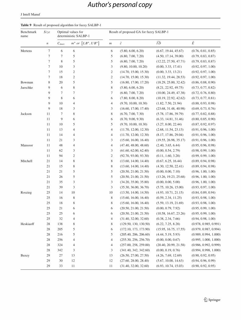
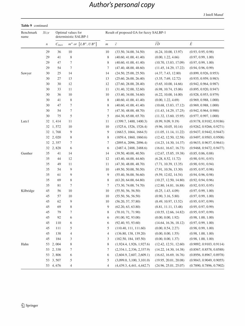
As it can be observed in Figs. 9, 10, 11, 12 and 13, theproposed method is convergent into better solution for stan-dard function in comparison with others barring Tournamentin Sphere. Moreover, it has partly better convergence rate.Here, the convergence rate of proposed algorithm is betterthan Random and Roulette Wheel but rather than Tourna-ment it lowers in some of functions. As mentioned before,focusing on diversity and convergence makes the conver-gence rate lessen and stopping algorithm in local solutionrespectively. Tournament method in rather to the proposedalgorithm has more focus on convergence that this tends toboosting in convergence rate and also make ceasing Tourna-

Table 4 Standard function (Molga and Smutnicki 2005)

Row Test function’s name Test function

1 De Jong’s function (sphere model) f (x) = ∑ni=1 x2

i ,−10 ≤ xi ≤ 10, i = 1 . . . n; (n = 5) Global minimum f (x) = 0is obtainable for xi = 0, i = 1 . . . n

2 Rosenbrock’s Valley f (x) = ∑n−1i=1

{100 ∗ (

xi+1 − x2i

)2 + (1 − x2

i

)2},−3 ≤ xi ≤ 3, i =

1 . . . n; (n = 5) Global minimum f (x) = 0 is obtainable for xi = 0, i = 1 . . . n

3 Goldstein-Price’s function f (x) = {1 + (x + y + 1)2 .

(19 − 14x + 3x2 − 14y + 6xy + 3y2

)} ·{30 + (2x − 3y)2 · (18 − 32x + 12x2 + 48y − 36xy + 27y2

)},−2 ≤ x, y ≤ 2,

Global minimum f (x) = 3 is obtainable for (x, y) = (0,−1)

4 Ackley’s function f (x) = −ae−b√

1n

∑ni=1 x2

i −e

{1n

∑ni=1 cos(cxi )

}

+a+e a = 20, b = 0.2, c = 2π,−5 ≤xi ≤ 5, i = 1 . . . n, (n = 5) Global minimum f (x) = 0 is obtainable for xi = 0, i =1 . . . n

5 Easom’s function f (x) = −cos (x)·cos (y)·e−{(x−π)2+(y−π)2}

,−100 ≤ x, y ≤ 100, Global minimumf (x) = −1 is obtainable for (x, y) = (π, π)

Table 5 Methods details

Selection method Parent selection New generation

Roulette Wheel Roulette Wheel (fitness proportion selection) Roulette Wheel & elitism selection

Tournament Tournament tournament & elitism selection

Random Random selection Random selection & archive

One-fifth success rule Fitness proportion selection and none-liner scalingusing one-fifth success rule

Selection base scaled fitness proportion & elitismselection

Fig. 9 Algorithms results forDe Jong’s function

-25

-20

-15

-10

-5

0

5

1 1001 2001 3001 4001 5001 6001 7001 8001 9001

Obj

ec�v

e(L

og(z

))

Itera�on

Proposed Algo�rthm Roule�e Wheel Tournament Random

123


J Intell Manuf

Fig. 10 Algorithms results forRosenbrock’s Valley function

-1

-0.5

0

0.5

1

1.5

2

2.5

1 1001 2001 3001 4001 5001 6001 7001 8001 9001 10001

Obj

ec�v

e(L

og(z

))Itera�on


Fig. 11 Algorithms results forGoldstein-Price’s function

0

0.2

0.4

0.6

0.8

1

1.2

1.4

1.6

1 6 11 16 21 26

Obj

ec�v

e(L

og(z

))

Itera�onProposed Algo�rthm Roule�e Wheel Tournament Random

Fig. 12 Algorithms results forAckley’s function

-16

-14

-12

-10

-8

-6

-4

-2

0

2

1 11 21 31 41 51 61 71 81 91 101 111 121 131 141 151 161 171 181 191 201 211

Obj

ec�v

e(L

og(z

))

Itera�onProposed Algo�rthm Roule�e Wheel Tournament Random

ment in local solution more possible. In another word, lowfocus on the diversity is the main cause of Tournament worstresults in comparison with proposed algorithm.

Numerical results over SALBP-1 and SULBP-1benchmarks

In this section the proposed algorithm will examine on thebenchmarks of SALBP-1 and SULBP-1. More details ofthese benchmarks are reachable on Scholl (1993) and http://alb.mansci.de. These benchmarks have defined in crisp state,

so for transfer that to fuzzy state, postulated that input num-ber in crisp state equals to peak point (A2) in fuzzy state.For calculation of beginning point (A1) and end point (A3)

formula (1) come in hand. In this paper the value of ψ andχ for tasks processing time got used to be 0.1 and for Cmax

is 1.

A = (A2 − χ, A2, A2 + ψ) (30)

Selected benchmarks according to number of tasks (n)are divided into A, B, & C. These groups consist of

123


http://alb.mansci.de

http://alb.mansci.de

J Intell Manuf

Fig. 13 Algorithms results forEasom’s function

-1.20E+00

-1.00E+00

-8.00E-01

-6.00E-01

-4.00E-01

-2.00E-01

0.00E+00

1 6 11 16 21 26

Obj

ec�v

e(L

og(z

))Itera�on


Table 6 Selected benchmarks for each class (A, B, C)

Class A Class B Class C

Benchmark name Benchmark size Benchmark name Benchmark size Benchmark name Benchmark size

Mertens 7 Roszieg 25 Kilbridge 45

Bowman 8 Heskiaoff 28 Hahn 53

Jaeschke 9 Buxey 29 Warnecke 58

Jackson 11 Sawyer 30 Tonge 70

Mansoor 11 Lutz1 32 Wee-Mag 75

Mitchell 21 Gunther 35 Arcus1 83

Table 7 Summarized reached solutions for SALBP-1

Problem class Average of %Deviation %Optimal solution

Class A 0.00 100

Class B 1.42 90.61

Class C 2.65 63.75

Total 1.36 84.79

small-sized benchmarks (n < 25), medium-sized bench-marks (25 ≤ n < 45), and big-sized benchmarks (n ≥ 45)respectively. Selected benchmarks for each class are show inTable 6.

The proposed algorithm implemented in MATLAB andrun on a computer with “Core 2 Duo 2.2, 2 GHz PC”. Becauseof stochastic behavior in meta-heuristic algorithm, the algo-rithm was tried out 10 runs by each benchmark and the bestsolutions summarized in Tables 7 and 8. Output solutionscompared with optimums by formula (31).

%Deviation ={(x − x∗)

x

∗}· 100 (31)

Tables 7 and 8 consist of below information:

• Average of %Deviation: shows the average percent ofdeviations.

Table 8 Summarized reached solutions for SULBP-1

Problem class Average of %Deviation %Optimal solution

Class A 0.00 100

Class B 3.32 71.16

Class C 3.80 58.26

Total 2.37 76.48

• %Optimal solution: expose the optimum solution per-centage.

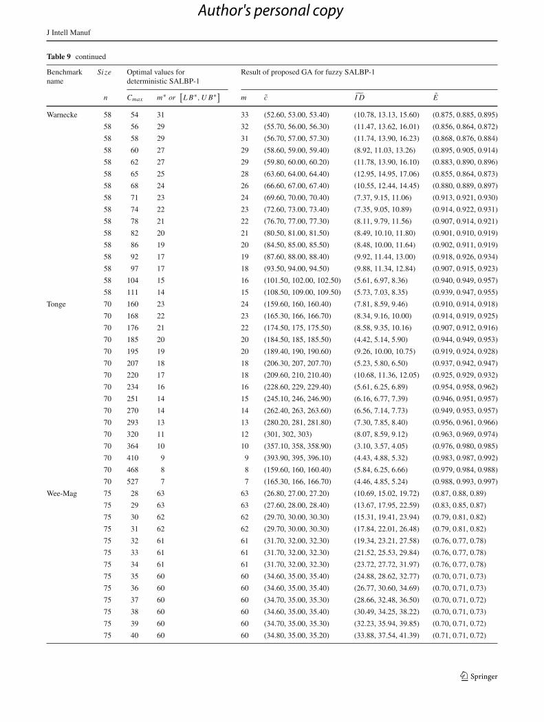
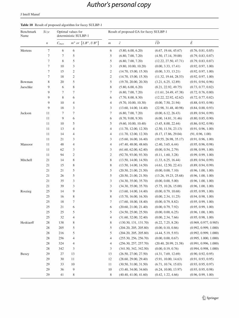
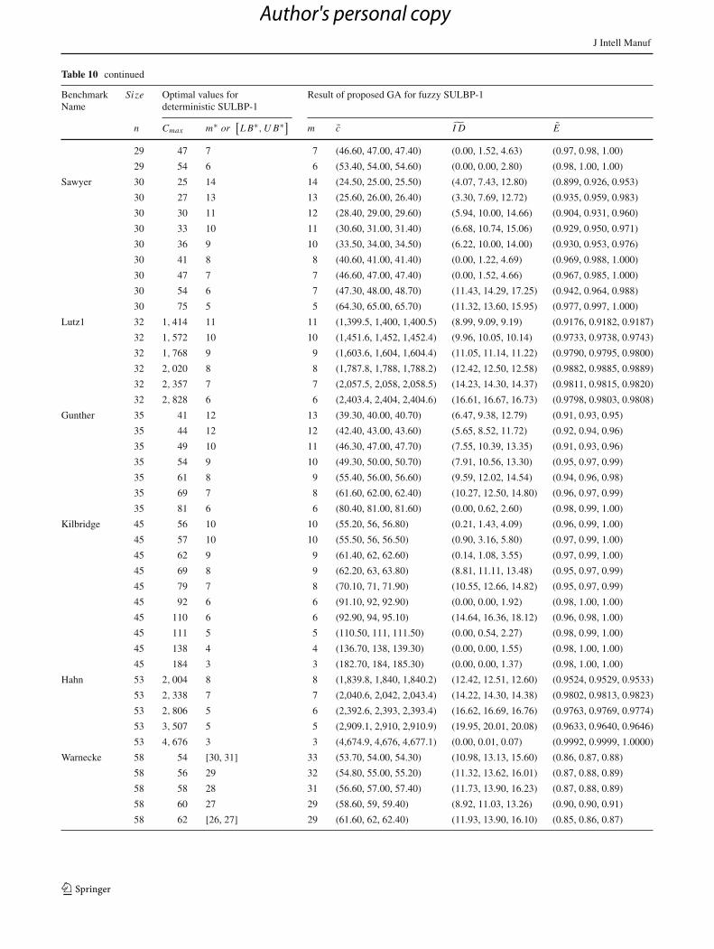
As cleared in Tables 7 and 8, proposed algorithm tends tothe optimum results in the all A class benchmarks that showsthe high performance of this algorithm for this class. Thebigger solution space, the lower solutions quality, and thisare clear in B and C classes. All in all proposed algorithmhas good performance in solving the class B and also goodin class C. In SALB-1 rather than SULB-1 has better resultrather than algorithm, that it is stem in smaller size of solutionspace, although the algorithm has high performance in bothof SALB-1 and SULB-1 whichever apparently presented inthe last row of Tables 7 and 8. More results exposed in detailsin Tables 9 and 10.

Run time depends to the problem size completely clear. Inanother word the more number of the tasks in ALBP the fur-ther computer run-time. The average CPU time for running

123


J Intell Manuf

Table 9 Result of proposed algorithm for fuzzy SALBP-1

Benchmarkname

Size Optimal values fordeterministic SALBP-1

Result of proposed GA for fuzzy SALBP-1

n Cmax m∗ or[L B∗,U B∗] m c I D E

Mertens 7 6 6 6 (5.80, 6.00, 6.20) (6.67, 19.44, 45.67) (0.76, 0.81, 0.85)

7 7 5 5 (6.80, 7.00, 7.20) (4.50, 17.14, 39.00) (0.79, 0.83, 0.87)

7 8 5 5 (6.80, 7.00, 7.20) (12.22, 27.50, 47.71) (0.79, 0.83, 0.87)

7 10 3 3 (9.80, 10.00, 10.20) (0.00, 3.33, 17.41) (0.92, 0.97, 1.00)

7 15 2 2 (14.70, 15.00, 15.30) (0.00, 3.33, 13.21) (0.92, 0.97, 1.00)

7 18 2 2 (14.70, 15.00, 15.30) (11.32, 19.44, 28.53) (0.92, 0.97, 1.00)

Bowman 8 20 5 5 (16.80, 17.00, 17.20) (18.29, 25.00, 32.42) (0.86, 0.88, 0.90)

Jaeschke 9 6 8 8 (5.80, 6.00, 6.20) (8.21, 22.92, 49.75) (0.73, 0.77, 0.82)

9 7 7 7 (6.80, 7.00, 7.20) (10.00, 24.49, 47.38) (0.72, 0.76, 0.80)

9 8 6 6 (7.80, 8.00, 8.20) (10.19, 22.92, 42.62) (0.73, 0.77, 0.81)

9 10 4 4 (9.70, 10.00, 10.30) (1.82, 7.50, 21.94) (0.88, 0.93, 0.98)

9 18 3 3 (16.60, 17.00, 17.40) (23.68, 31.48, 40.98) (0.69, 0.73, 0.76)

Jackson 11 7 8 8 (6.70, 7.00, 7.30) (5.78, 17.86, 39.79) (0.77, 0.82, 0.88)

11 9 6 6 (8.70, 9.00, 9.30) (6.33, 14.81, 31.46) (0.80, 0.85, 0.90)

11 10 5 5 (9.70, 10.00, 10.30) (3.27, 8.00, 22.44) (0.87, 0.92, 0.97)

11 13 4 4 (11.70, 12.00, 12.30) (2.68, 11.54, 23.13) (0.91, 0.96, 1.00)

11 14 4 4 (11.70, 12.00, 12.30) (8.17, 17.86, 29.04) (0.91, 0.96, 1.00)

11 21 3 3 (15.60, 16.00, 16.40) (19.55, 26.98, 35.17) (0.91, 0.96, 1.00)

Mansoor 11 48 4 4 (47.40, 48.00, 48.60) (2.40, 3.65, 6.44) (0.95, 0.96, 0.98)

11 62 3 3 (61.60, 62.00, 62.40) (0.00, 0.54, 2.79) (0.98, 0.99, 1.00)

11 94 2 2 (92.70, 93.00, 93.30) (0.11, 1.60, 3.28) (0.99, 0.99, 1.00)

Mitchell 21 14 8 8 (13.60, 14.00, 14.40) (0.67, 6.25, 16.44) (0.89, 0.94, 0.98)

21 15 8 8 (13.60, 14.00, 14.40) (4.30, 12.50, 22.41) (0.89, 0.94, 0.98)

21 21 5 5 (20.50, 21.00, 21.50) (0.00, 0.00, 7.10) (0.96, 1.00, 1.00)

21 26 5 5 (20.50, 21.00, 21.50) (13.26, 19.23, 25.68) (0.96, 1.00, 1.00)

21 35 3 3 (34.20, 35.00, 35.80) (0.00, 0.00, 5.00) (0.96, 1.00, 1.00)

21 39 3 3 (35.30, 36.00, 36.70) (5.75, 10.26, 15.00) (0.93, 0.97, 1.00)

Roszieg 25 14 10 10 (13.50, 14.00, 14.50) (4.93, 10.71, 21.15) (0.84, 0.89, 0.94)

25 16 8 8 (15.60, 16.00, 16.40) (0.59, 2.34, 11.25) (0.93, 0.98, 1.00)

25 18 8 8 (15.60, 16.00, 16.40) (5.59, 13.19, 21.69) (0.93, 0.98, 1.00)

25 21 6 6 (20.50, 21.00, 21.50) (0.00, 0.79, 7.92) (0.95, 0.99, 1.00)

25 25 6 6 (20.50, 21.00, 21.50) (10.58, 16.67, 23.26) (0.95, 0.99, 1.00)

25 32 4 4 (31.40, 32.00, 32.60) (0.38, 2.34, 7.66) (0.94, 0.98, 1.00)

Heskiaoff 28 138 8 8 (129.50, 130, 130.50) (6.22, 7.25, 8.28) (0.978, 0.985, 0.991)

28 205 5 6 (172.10, 173, 173.90) (15.95, 16.75, 17.55) (0.979, 0.987, 0.994)

28 216 5 5 (205.40, 206, 206.60) (4.44, 5.19, 5.93) (0.989, 0.994, 1.000)

28 256 4 4 (255.30, 256, 256.70) (0.00, 0.00, 0.67) (0.995, 1.000, 1.000)

28 324 4 4 (257.00, 258, 259.00) (20.40, 20.99, 21.58) (0.986, 0.992, 0.999)

28 342 3 3 (341.40, 342, 342.60) (0.00, 0.19, 0.76) (0.994, 0.998, 1.000)

Buxey 29 27 13 13 (26.50, 27.00, 27.50) (4.26, 7.69, 12.69) (0.90, 0.92, 0.95)

29 30 12 12 (27.60, 28.00, 28.40) (5.67, 10.00, 14.63) (0.94, 0.96, 0.99)

29 33 11 11 (31.40, 32.00, 32.60) (6.93, 10.74, 15.03) (0.90, 0.92, 0.95)

123


J Intell Manuf

Table 9 continued

Benchmarkname




29 36 10 10 (33.50, 34.00, 34.50) (6.24, 10.00, 13.97) (0.93, 0.95, 0.98)

29 41 8 8 (40.60, 41.00, 41.40) (0.00, 1.22, 4.66) (0.97, 0.99, 1.00)

29 47 7 8 (40.60, 41.00, 41.40) (10.70, 13.83, 17.09) (0.97, 0.99, 1.00)

29 54 7 7 (47.40, 48.00, 48.60) (11.45, 14.29, 17.22) (0.94, 0.96, 0.99)

Sawyer 30 25 14 14 (24.50, 25.00, 25.50) (4.37, 7.43, 12.80) (0.899, 0.926, 0.953)

30 27 13 13 (25.60, 26.00, 26.40) (3.35, 7.69, 12.72) (0.935, 0.959, 0.983)

30 30 12 12 (27.60, 28.00, 28.40) (5.65, 10.00, 14.66) (0.942, 0.964, 0.987)

30 33 11 11 (31.40, 32.00, 32.60) (6.98, 10.74, 15.06) (0.895, 0.920, 0.947)

30 36 10 10 (33.40, 34.00, 34.60) (6.22, 10.00, 14.00) (0.928, 0.953, 0.979)

30 41 8 8 (40.60, 41.00, 41.40) (0.00, 1.22, 4.69) (0.969, 0.988, 1.000)

30 47 7 8 (40.60, 41.00, 41.40) (10.68, 13.83, 17.12) (0.969, 0.988, 1.000)

30 54 7 7 (47.30, 48.00, 48.70) (11.43, 14.29, 17.25) (0.942, 0.964, 0.988)

30 75 5 5 (64.30, 65.00, 65.70) (11.32, 13.60, 15.95) (0.977, 0.997, 1.000)

Lutz1 32 1, 414 11 11 (1399.7, 1400, 1400.3) (8.99, 9.09, 9.19) (0.9178, 0.9182, 0.9186)

32 1, 572 10 10 (1525.6, 1526, 1526.4) (9.96, 10.05, 10.14) (0.9262, 0.9266, 0.9271)

32 1, 768 9 9 (1663.5, 1664, 1664.5) (11.05, 11.14, 11.22) (0.9437, 0.9442, 0.9447)

32 2, 020 8 8 (1859.4, 1860, 1860.6) (12.42, 12.50, 12.58) (0.9497, 0.9503, 0.9508)

32 2, 357 7 7 (2095.6, 2096, 2096.4) (14.23, 14.30, 14.37) (0.9633, 0.9637, 0.9641)

32 2, 828 6 6 (2487.4, 2488, 2488.6) (16.61, 16.67, 16.73) (0.9468, 0.9472, 0.9477)

Gunther 35 41 14 14 (39.50, 40.00, 40.50) (12.67, 15.85, 19.38) (0.85, 0.86, 0.88)

35 44 12 12 (43.40, 44.00, 44.60) (6.28, 8.52, 11.72) (0.90, 0.91, 0.93)

35 49 11 11 (47.30, 48.00, 48.70) (7.71, 10.39, 13.35) (0.90, 0.91, 0.94)

35 54 9 10 (49.50, 50.00, 50.50) (7.91, 10.56, 13.30) (0.95, 0.97, 0.98)

35 61 9 9 (55.40, 56.00, 56.60) (9.59, 12.02, 14.54) (0.94, 0.96, 0.98)

35 69 8 8 (63.20, 64.00, 64.80) (10.27, 12.50, 14.80) (0.92, 0.94, 0.96)

35 81 7 7 (73.30, 74.00, 74.70) (12.80, 14.81, 16.88) (0.92, 0.93, 0.95)

Kilbridge 45 56 10 10 (55.50, 56, 56.50) (0.25, 1.43, 4.09) (0.97, 0.99, 1.00)

45 57 10 10 (55.50, 56, 56.50) (0.90, 3.16, 5.80) (0.97, 0.99, 1.00)

45 62 9 10 (56.20, 57, 57.80) (8.49, 10.97, 13.52) (0.95, 0.97, 0.99)

45 69 8 9 (62.20, 63, 63.80) (8.81, 11.11, 13.48) (0.95, 0.97, 0.99)

45 79 7 8 (70.10, 71, 71.90) (10.55, 12.66, 14.82) (0.95, 0.97, 0.99)

45 92 6 6 (91.00, 92, 93.00) (0.00, 0.00, 1.92) (0.98, 1.00, 1.00)

45 110 6 6 (92.40, 93, 93.60) (14.64, 16.36, 18.12) (0.97, 0.99, 1.00)

45 111 5 5 (110.40, 111, 111.60) (0.00, 0.54, 2.27) (0.98, 0.99, 1.00)

45 138 4 4 (136.80, 138, 139.20) (0.00, 0.00, 1.55) (0.98, 1.00, 1.00)

45 184 3 3 (182.50, 184, 185.50) (0.00, 0.00, 1.37) (0.98, 1.00, 1.00)

Hahn 53 2, 004 8 8 (1,924.4, 1,926, 1,927.6) (12.42, 12.51, 12.60) (0.9092, 0.9103, 0.9114)

53 2, 338 7 7 (2,334.1, 2,336, 2,337.9) (14.22, 14.30, 14.38) (0.8567, 0.8578, 0.8588)

53 2, 806 6 6 (2,604.9, 2,607, 2,609.1) (16.62, 16.69, 16.76) (0.8956, 0.8967, 0.8978)

53 3, 507 5 5 (3,099.0, 3,100, 3,101.0) (19.95, 20.01, 20.08) (0.9043, 0.9049, 0.9055)

53 4, 676 4 4 (4,439.3, 4,441, 4,442.7) (24.96, 25.01, 25.07) (0.7890, 0.7896, 0.7902)

123


J Intell Manuf

Table 9 continued

Benchmarkname




Warnecke 58 54 31 33 (52.60, 53.00, 53.40) (10.78, 13.13, 15.60) (0.875, 0.885, 0.895)

58 56 29 32 (55.70, 56.00, 56.30) (11.47, 13.62, 16.01) (0.856, 0.864, 0.872)

58 58 29 31 (56.70, 57.00, 57.30) (11.74, 13.90, 16.23) (0.868, 0.876, 0.884)

58 60 27 29 (58.60, 59.00, 59.40) (8.92, 11.03, 13.26) (0.895, 0.905, 0.914)

58 62 27 29 (59.80, 60.00, 60.20) (11.78, 13.90, 16.10) (0.883, 0.890, 0.896)

58 65 25 28 (63.60, 64.00, 64.40) (12.95, 14.95, 17.06) (0.855, 0.864, 0.873)

58 68 24 26 (66.60, 67.00, 67.40) (10.55, 12.44, 14.45) (0.880, 0.889, 0.897)

58 71 23 24 (69.60, 70.00, 70.40) (7.37, 9.15, 11.06) (0.913, 0.921, 0.930)

58 74 22 23 (72.60, 73.00, 73.40) (7.35, 9.05, 10.89) (0.914, 0.922, 0.931)

58 78 21 22 (76.70, 77.00, 77.30) (8.11, 9.79, 11.56) (0.907, 0.914, 0.921)

58 82 20 21 (80.50, 81.00, 81.50) (8.49, 10.10, 11.80) (0.901, 0.910, 0.919)

58 86 19 20 (84.50, 85.00, 85.50) (8.48, 10.00, 11.64) (0.902, 0.911, 0.919)

58 92 17 19 (87.60, 88.00, 88.40) (9.92, 11.44, 13.00) (0.918, 0.926, 0.934)

58 97 17 18 (93.50, 94.00, 94.50) (9.88, 11.34, 12.84) (0.907, 0.915, 0.923)

58 104 15 16 (101.50, 102.00, 102.50) (5.61, 6.97, 8.36) (0.940, 0.949, 0.957)

58 111 14 15 (108.50, 109.00, 109.50) (5.73, 7.03, 8.35) (0.939, 0.947, 0.955)

Tonge 70 160 23 24 (159.60, 160, 160.40) (7.81, 8.59, 9.46) (0.910, 0.914, 0.918)

70 168 22 23 (165.30, 166, 166.70) (8.34, 9.16, 10.00) (0.914, 0.919, 0.925)

70 176 21 22 (174.50, 175, 175.50) (8.58, 9.35, 10.16) (0.907, 0.912, 0.916)

70 185 20 20 (184.50, 185, 185.50) (4.42, 5.14, 5.90) (0.944, 0.949, 0.953)

70 195 19 20 (189.40, 190, 190.60) (9.26, 10.00, 10.75) (0.919, 0.924, 0.928)

70 207 18 18 (206.30, 207, 207.70) (5.23, 5.80, 6.50) (0.937, 0.942, 0.947)

70 220 17 18 (209.60, 210, 210.40) (10.68, 11.36, 12.05) (0.925, 0.929, 0.932)

70 234 16 16 (228.60, 229, 229.40) (5.61, 6.25, 6.89) (0.954, 0.958, 0.962)

70 251 14 15 (245.10, 246, 246.90) (6.16, 6.77, 7.39) (0.946, 0.951, 0.957)

70 270 14 14 (262.40, 263, 263.60) (6.56, 7.14, 7.73) (0.949, 0.953, 0.957)

70 293 13 13 (280.20, 281, 281.80) (7.30, 7.85, 8.40) (0.956, 0.961, 0.966)

70 320 11 12 (301, 302, 303) (8.07, 8.59, 9.12) (0.963, 0.969, 0.974)

70 364 10 10 (357.10, 358, 358.90) (3.10, 3.57, 4.05) (0.976, 0.980, 0.985)

70 410 9 9 (393.90, 395, 396.10) (4.43, 4.88, 5.32) (0.983, 0.987, 0.992)

70 468 8 8 (159.60, 160, 160.40) (5.84, 6.25, 6.66) (0.979, 0.984, 0.988)

70 527 7 7 (165.30, 166, 166.70) (4.46, 4.85, 5.24) (0.988, 0.993, 0.997)

Wee-Mag 75 28 63 63 (26.80, 27.00, 27.20) (10.69, 15.02, 19.72) (0.87, 0.88, 0.89)

75 29 63 63 (27.60, 28.00, 28.40) (13.67, 17.95, 22.59) (0.83, 0.85, 0.87)

75 30 62 62 (29.70, 30.00, 30.30) (15.31, 19.41, 23.94) (0.79, 0.81, 0.82)

75 31 62 62 (29.70, 30.00, 30.30) (17.84, 22.01, 26.48) (0.79, 0.81, 0.82)

75 32 61 61 (31.70, 32.00, 32.30) (19.34, 23.21, 27.58) (0.76, 0.77, 0.78)

75 33 61 61 (31.70, 32.00, 32.30) (21.52, 25.53, 29.84) (0.76, 0.77, 0.78)

75 34 61 61 (31.70, 32.00, 32.30) (23.72, 27.72, 31.97) (0.76, 0.77, 0.78)

75 35 60 60 (34.60, 35.00, 35.40) (24.88, 28.62, 32.77) (0.70, 0.71, 0.73)

75 36 60 60 (34.60, 35.00, 35.40) (26.77, 30.60, 34.69) (0.70, 0.71, 0.73)

75 37 60 60 (34.70, 35.00, 35.30) (28.66, 32.48, 36.50) (0.70, 0.71, 0.72)

75 38 60 60 (34.60, 35.00, 35.40) (30.49, 34.25, 38.22) (0.70, 0.71, 0.73)

75 39 60 60 (34.70, 35.00, 35.30) (32.23, 35.94, 39.85) (0.70, 0.71, 0.72)

75 40 60 60 (34.80, 35.00, 35.20) (33.88, 37.54, 41.39) (0.71, 0.71, 0.72)

123


J Intell Manuf

Table 9 continued

Benchmarkname




75 41 59 59 (40.50, 41.00, 41.50) (34.55, 38.03, 41.80) (0.61, 0.62, 0.63)

75 42 55 55 (41.70, 42.00, 42.30) (31.96, 35.11, 38.74) (0.64, 0.65, 0.66)

75 43 50 50 (42.70, 43.00, 43.30) (27.54, 30.28, 33.74) (0.69, 0.70, 0.71)

75 47 33 35 (46.70, 47.00, 47.30) (6.90, 8.88, 11.71) (0.90, 0.91, 0.92)

75 49 32 33 (48.70, 49.00, 49.30) (5.24, 7.30, 10.01) (0.92, 0.93, 0.94)

75 50 32 33 (48.60, 49.00, 49.40) (6.65, 9.15, 11.84) (0.91, 0.93, 0.94)

75 52 31 32 (50.60, 51.00, 51.40) (7.45, 9.92, 12.53) (0.91, 0.92, 0.93)

75 54 31 31 (52.60, 53.00, 53.40) (8.06, 10.45, 12.99) (0.90, 0.91, 0.92)

75 56 30 30 (55.70, 56.00, 56.30) (8.75, 10.77, 13.24) (0.88, 0.89, 0.90)

Arcus1 83 3, 786 21 22 (3,690.9, 3,691, 3,691.1) (9.07, 9.11, 9.15) (0.9322, 0.9323, 0.9325)

83 3, 985 20 21 (3,857.5, 3,858, 3,858.5) (9.50, 9.53, 9.57) (0.9342, 0.9344, 0.9347)

83 4, 206 19 19 (4,177.4, 4,178, 4,178.6) (5.23, 5.26, 5.30) (0.9535, 0.9537, 0.9539)

83 4, 454 18 19 (4,241.6, 4,242, 4,242.4) (10.50, 10.54, 10.57) (0.9391, 0.9393, 0.9395)

83 4, 732 17 17 (4,678.6, 4,679, 4,679.4) (5.86, 5.89, 5.92) (0.9516, 0.9518, 0.9520)

83 5, 048 16 16 (4,954.3, 4,955, 4,955.7) (6.23, 6.27, 6.30) (0.9547, 0.9549, 0.9552)

83 5, 408 15 15 (5,281.5, 5,282, 5,282.5) (6.64, 6.67, 6.70) (0.9553, 0.9555, 0.9557)

83 5, 824 14 14 (5,565.5, 5,566, 5,566.5) (7.12, 7.15, 7.18) (0.9714, 0.9715, 0.9717)

83 5, 853 14 14 (5,599.3, 5,600, 5,600.7) (7.58, 7.61, 7.64) (0.9654, 0.9657, 0.9659)

83 6, 309 13 13 (6,042.2, 6,043, 6,043.8) (7.67, 7.69, 7.72) (0.9635, 0.9637, 0.9639)

83 6, 842 12 12 (6,508.9, 6,510, 6,511.1) (7.77, 7.79, 7.82) (0.9688, 0.9691, 0.9694)

83 6, 883 12 12 (6,561.5, 6,562, 6,562.5) (8.31, 8.34, 8.37) (0.9613, 0.9614, 0.9616)

83 7, 571 11 11 (7,090.7, 7,091, 7,091.3) (9.07, 9.09, 9.12) (0.9704, 0.9706, 0.9707)

83 8, 412 10 10 (7,921.8, 7,923, 7,924.2) (9.98, 10.00, 10.02) (0.9553, 0.9555, 0.9558)

83 8, 898 9 9 (8,527.4, 8,528, 8,528.6) (5.44, 5.46, 5.49) (0.9862, 0.9864, 0.9866)

8310, 816 8 8 (10,220.6, 10,222, 10,223.4) (12.49, 12.51, 12.53) (0.9256, 0.9258, 0.9260)

each benchmark have exposed in Fig.14. As cleared, processtime varies between 3 and 360 s that proofs algorithm valu-able convergence time.

Final comparison between proposed method and existingmethods

In this section, performance of the proposed algorithm isexamined using (Tsujimura et al. 1995) test problem. Anexample of the problem is solved by the proposed algorithmto illustrate the improvements and the results compared withexisting methods in this problem that is presented in Table 11,and finally the predecessor and successor constraints of thetest problem are displayed in Fig. 15.

The population and generation size of the algorithmdefined in small scale because of the size of this exampleand power of the algorithm. The size of population is equalto 3 and the number of maximum generation is limited to

5. The best obtained solution for fuzzy efficiency and fuzzyidle time for SALB is as follow:

• Fuzzy efficiency = [0.73, 0.97, 1]• Fuzzy idle percentage = [3.92, 16.67, 34.01]

Best solution for SULB is as follows:

• Fuzzy efficiency = [0.73, 0.99, 1]• Fuzzy idle percentage = [3.92, 16.67, 34.01]

Commonly from every three run times of the algorithm, oncewill converge to the best obtained solution. The results fromthe proposed algorithm and the results from other existingmethods are shown in Table 12. The first and second rows ofthe Table 12 present the results from the proposed algorithmin this paper for SALB and SULB, respectively. The thirdrow of the table shows the results from the GA offered by

123


J Intell Manuf

Table 10 Result of proposed algorithm for fuzzy SULBP-1

BenchmarkName

Size Optimal values fordeterministic SULBP-1

Result of proposed GA for fuzzy SULBP-1


Mertens 7 6 6 6 (5.80, 6.00, 6.20) (6.67, 19.44, 45.67) (0.76, 0.81, 0.85)

7 7 5 5 (6.80, 7.00, 7.20) (4.50, 17.14, 39.00) (0.79, 0.83, 0.87)

7 8 5 5 (6.80, 7.00, 7.20) (12.22, 27.50, 47.71) (0.79, 0.83, 0.87)

7 10 3 3 (9.80, 10.00, 10.20) (0.00, 3.33, 17.41) (0.92, 0.97, 1.00)

7 15 2 2 (14.70, 15.00, 15.30) (0.00, 3.33, 13.21) (0.92, 0.97, 1.00)

7 18 2 2 (14.70, 15.00, 15.30) (11.32, 19.44, 28.53) (0.92, 0.97, 1.00)

Bowman 8 20 5 5 (19.70, 20.00, 20.30) (3.21, 6.25, 12.89) (0.91, 0.94, 0.96)

Jaeschke 9 6 8 8 (5.80, 6.00, 6.20) (8.21, 22.92, 49.75) (0.73, 0.77, 0.82)

9 7 7 7 (6.80, 7.00, 7.20) (11.61, 24.49, 47.38) (0.72, 0.76, 0.80)

9 8 6 6 (7.70, 8.00, 8.30) (12.22, 22.92, 42.62) (0.72, 0.77, 0.82)

9 10 4 4 (9.70, 10.00, 10.30) (0.00, 7.50, 21.94) (0.88, 0.93, 0.98)

9 18 3 3 (13.60, 14.00, 14.40) (22.98, 31.48, 40.98) (0.84, 0.88, 0.93)

Jackson 11 7 7 7 (6.80, 7.00, 7.20) (0.00, 6.12, 26.43) (0.89, 0.94, 0.99)

11 9 6 6 (8.70, 9.00, 9.30) (6.00, 14.81, 31.46) (0.80, 0.85, 0.90)

11 10 5 5 (9.60, 10.00, 10.40) (3.45, 8.00, 22.44) (0.86, 0.92, 0.98)

11 13 4 4 (11.70, 12.00, 12.30) (2.50, 11.54, 23.13) (0.91, 0.96, 1.00)

11 14 4 4 (11.70, 12.00, 12.30) (8.17, 17.86, 29.04) (91, 0.96, 1.00)

11 21 3 3 (15.60, 16.00, 16.40) (19.55, 26.98, 35.17) (0.91, 0.96, 1.00)

Mansoor 11 48 4 4 (47.40, 48.00, 48.60) (2.40, 3.65, 6.44) (0.95, 0.96, 0.98)

11 62 3 3 (61.60, 62.00, 62.40) (0.00, 0.54, 2.79) (0.98, 0.99, 1.00)

11 94 2 2 (92.70, 93.00, 93.30) (0.11, 1.60, 3.28) (0.99, 0.99, 1.00)

Mitchell 21 14 8 8 (13.50, 14.00, 14.50) (1.33, 6.25, 16.44) (0.89, 0.94, 0.99)

21 15 8 8 (13.50, 14.00, 14.50) (4.61, 12.50, 22.41) (0.89, 0.94, 0.99)

21 21 5 5 (20.50, 21.00, 21.50) (0.00, 0.00, 7.10) (0.96, 1.00, 1.00)

21 26 5 5 (20.50, 21.00, 21.50) (13.26, 19.23, 25.68) (0.96, 1.00, 1.00)

21 35 3 3 (34.30, 35.00, 35.70) (0.00, 0.00, 5.00) (0.96, 1.00, 1.00)

21 39 3 3 (34.30, 35.00, 35.70) (5.75, 10.26, 15.00) (0.96, 1.00, 1.00)

Roszieg 25 14 9 9 (13.60, 14.00, 14.40) (0.00, 0.79, 10.68) (0.95, 0.99, 1.00)

25 16 8 8 (15.70, 16.00, 16.30) (0.00, 2.34, 11.25) (0.94, 0.98, 1.00)

25 18 7 7 (17.60, 18.00, 18.40) (0.00, 0.79, 8.82) (0.95, 0.99, 1.00)

25 21 6 6 (20.60, 21.00, 21.40) (0.00, 0.79, 7.92) (0.95, 0.99, 1.00)

25 25 5 5 (24.50, 25.00, 25.50) (0.00, 0.00, 6.25) (0.96, 1.00, 1.00)

25 32 4 4 (31.60, 32.00, 32.40) (0.00, 2.34, 7.66) (0.95, 0.98, 1.00)

Heskiaoff 28 138 8 8 (130.30, 131, 131.70) (6.22, 7.25, 8.28) (0.969, 0.977, 0.985)

28 205 5 5 (204.20, 205, 205.80) (0.00, 0.10, 0.86) (0.992, 0.999, 1.000)

28 216 5 5 (204.20, 205, 205.80) (4.44, 5.19, 5.93) (0.992, 0.999, 1.000)

28 256 4 4 (255.30, 256, 256.70) (0.00, 0.00, 0.67) (0.995, 1.000, 1.000)

28 324 4 4 (256.30, 257, 257.70) (20.40, 20.99, 21.58) (0.991, 0.996, 1.000)

28 342 3 3 (341.50, 342, 342.50) (0.00, 0.19, 0.76) (0.994, 0.998, 1.000)

Buxey 29 27 13 13 (26.50, 27.00, 27.50) (4.31, 7.69, 12.69) (0.90, 0.92, 0.95)

29 30 11 12 (28.60, 29.00, 29.40) (5.91, 10.00, 14.63) (0.91, 0.93, 0.95)

29 33 10 11 (30.50, 31.00, 31.50) (6.71, 10.74, 15.03) (0.93, 0.95, 0.97)

29 36 9 10 (33.40, 34.00, 34.60) (6.24, 10.00, 13.97) (0.93, 0.95, 0.98)

29 41 8 8 (40.40, 41.00, 41.60) (0.42, 1.22, 4.66) (0.96, 0.99, 1.00)

123


J Intell Manuf

Table 10 continued

BenchmarkName




29 47 7 7 (46.60, 47.00, 47.40) (0.00, 1.52, 4.63) (0.97, 0.98, 1.00)

29 54 6 6 (53.40, 54.00, 54.60) (0.00, 0.00, 2.80) (0.98, 1.00, 1.00)

Sawyer 30 25 14 14 (24.50, 25.00, 25.50) (4.07, 7.43, 12.80) (0.899, 0.926, 0.953)

30 27 13 13 (25.60, 26.00, 26.40) (3.30, 7.69, 12.72) (0.935, 0.959, 0.983)

30 30 11 12 (28.40, 29.00, 29.60) (5.94, 10.00, 14.66) (0.904, 0.931, 0.960)

30 33 10 11 (30.60, 31.00, 31.40) (6.68, 10.74, 15.06) (0.929, 0.950, 0.971)

30 36 9 10 (33.50, 34.00, 34.50) (6.22, 10.00, 14.00) (0.930, 0.953, 0.976)

30 41 8 8 (40.60, 41.00, 41.40) (0.00, 1.22, 4.69) (0.969, 0.988, 1.000)

30 47 7 7 (46.60, 47.00, 47.40) (0.00, 1.52, 4.66) (0.967, 0.985, 1.000)

30 54 6 7 (47.30, 48.00, 48.70) (11.43, 14.29, 17.25) (0.942, 0.964, 0.988)

30 75 5 5 (64.30, 65.00, 65.70) (11.32, 13.60, 15.95) (0.977, 0.997, 1.000)

Lutz1 32 1, 414 11 11 (1,399.5, 1,400, 1,400.5) (8.99, 9.09, 9.19) (0.9176, 0.9182, 0.9187)

32 1, 572 10 10 (1,451.6, 1,452, 1,452.4) (9.96, 10.05, 10.14) (0.9733, 0.9738, 0.9743)

32 1, 768 9 9 (1,603.6, 1,604, 1,604.4) (11.05, 11.14, 11.22) (0.9790, 0.9795, 0.9800)

32 2, 020 8 8 (1,787.8, 1,788, 1,788.2) (12.42, 12.50, 12.58) (0.9882, 0.9885, 0.9889)

32 2, 357 7 7 (2,057.5, 2,058, 2,058.5) (14.23, 14.30, 14.37) (0.9811, 0.9815, 0.9820)

32 2, 828 6 6 (2,403.4, 2,404, 2,404.6) (16.61, 16.67, 16.73) (0.9798, 0.9803, 0.9808)

Gunther 35 41 12 13 (39.30, 40.00, 40.70) (6.47, 9.38, 12.79) (0.91, 0.93, 0.95)

35 44 12 12 (42.40, 43.00, 43.60) (5.65, 8.52, 11.72) (0.92, 0.94, 0.96)

35 49 10 11 (46.30, 47.00, 47.70) (7.55, 10.39, 13.35) (0.91, 0.93, 0.96)

35 54 9 10 (49.30, 50.00, 50.70) (7.91, 10.56, 13.30) (0.95, 0.97, 0.99)

35 61 8 9 (55.40, 56.00, 56.60) (9.59, 12.02, 14.54) (0.94, 0.96, 0.98)

35 69 7 8 (61.60, 62.00, 62.40) (10.27, 12.50, 14.80) (0.96, 0.97, 0.99)

35 81 6 6 (80.40, 81.00, 81.60) (0.00, 0.62, 2.60) (0.98, 0.99, 1.00)

Kilbridge 45 56 10 10 (55.20, 56, 56.80) (0.21, 1.43, 4.09) (0.96, 0.99, 1.00)

45 57 10 10 (55.50, 56, 56.50) (0.90, 3.16, 5.80) (0.97, 0.99, 1.00)

45 62 9 9 (61.40, 62, 62.60) (0.14, 1.08, 3.55) (0.97, 0.99, 1.00)

45 69 8 9 (62.20, 63, 63.80) (8.81, 11.11, 13.48) (0.95, 0.97, 0.99)

45 79 7 8 (70.10, 71, 71.90) (10.55, 12.66, 14.82) (0.95, 0.97, 0.99)

45 92 6 6 (91.10, 92, 92.90) (0.00, 0.00, 1.92) (0.98, 1.00, 1.00)

45 110 6 6 (92.90, 94, 95.10) (14.64, 16.36, 18.12) (0.96, 0.98, 1.00)

45 111 5 5 (110.50, 111, 111.50) (0.00, 0.54, 2.27) (0.98, 0.99, 1.00)

45 138 4 4 (136.70, 138, 139.30) (0.00, 0.00, 1.55) (0.98, 1.00, 1.00)

45 184 3 3 (182.70, 184, 185.30) (0.00, 0.00, 1.37) (0.98, 1.00, 1.00)

Hahn 53 2, 004 8 8 (1,839.8, 1,840, 1,840.2) (12.42, 12.51, 12.60) (0.9524, 0.9529, 0.9533)

53 2, 338 7 7 (2,040.6, 2,042, 2,043.4) (14.22, 14.30, 14.38) (0.9802, 0.9813, 0.9823)

53 2, 806 5 6 (2,392.6, 2,393, 2,393.4) (16.62, 16.69, 16.76) (0.9763, 0.9769, 0.9774)

53 3, 507 5 5 (2,909.1, 2,910, 2,910.9) (19.95, 20.01, 20.08) (0.9633, 0.9640, 0.9646)

53 4, 676 3 3 (4,674.9, 4,676, 4,677.1) (0.00, 0.01, 0.07) (0.9992, 0.9999, 1.0000)

Warnecke 58 54 [30, 31] 33 (53.70, 54.00, 54.30) (10.98, 13.13, 15.60) (0.86, 0.87, 0.88)

58 56 29 32 (54.80, 55.00, 55.20) (11.32, 13.62, 16.01) (0.87, 0.88, 0.89)

58 58 28 31 (56.60, 57.00, 57.40) (11.73, 13.90, 16.23) (0.87, 0.88, 0.89)

58 60 27 29 (58.60, 59, 59.40) (8.92, 11.03, 13.26) (0.90, 0.90, 0.91)

58 62 [26, 27] 29 (61.60, 62, 62.40) (11.93, 13.90, 16.10) (0.85, 0.86, 0.87)

123


J Intell Manuf

Table 10 continued

BenchmarkName




58 65 [24, 25] 28 (62.70, 63, 63.30) (12.89, 14.95, 17.06) (0.87, 0.88, 0.89)

58 68 [23, 24] 25 (67.60, 68, 68.40) (7.43, 8.94, 10.91) (0.90, 0.91, 0.92)

58 71 [22, 23] 24 (69.60, 70, 70.40) (7.37, 9.15, 11.06) (0.91, 0.92, 0.93)

58 74 [21, 22] 23 (72.60, 73, 73.40) (7.35, 9.05, 10.89) (0.91, 0.92, 0.93)

58 78 20 22 (76.50, 77, 77.50) (8.10, 9.79, 11.56) (0.90, 0.91, 0.92)

58 82 [19, 20] 20 (81.60, 82, 82.40) (4.19, 5.61, 7.27) (0.94, 0.94, 0.95)

58 86 18 20 (84.60, 85, 85.40) (8.49, 10.00, 11.64) (0.90, 0.91, 0.92)

58 92 17 18 (91.60, 92, 92.40) (5.24, 6.52, 8.05) (0.93, 0.93, 0.94)

58 97 16 18 (92.60, 93, 93.40) (9.88, 11.34, 12.84) (0.92, 0.92, 0.93)

58 104 15 16 (101.50, 102, 102.50) (5.61, 6.97, 8.36) (0.94, 0.95, 0.96)

58 111 14 15 (108.40, 109, 109.60) (5.73, 7.03, 8.35) (0.94, 0.95, 0.96)

Tonge 70 160 [22, 23] 24 (0.921, 0.926, 0.930) (7.74, 8.59, 9.46) (0.921, 0.926, 0.930)

70 168 21 23 (0.910, 0.914, 0.917) (8.34, 9.16, 10.00) (0.910, 0.914, 0.917)

70 176 [20, 21] 22 (0.907, 0.912, 0.917) (8.57, 9.35, 10.16) (0.907, 0.912, 0.917)

70 185 19 20 (0.944, 0.949, 0.953) (4.42, 5.14, 5.90) (0.944, 0.949, 0.953)

70 195 18 20 (0.919, 0.924, 0.928) (9.26, 10.00, 10.75) (0.919, 0.924, 0.928)

70 207 17 18 (0.937, 0.942, 0.947) (5.23, 5.80, 6.50) (0.937, 0.942, 0.947)

70 220 16 17 (0.934, 0.939, 0.943) (5.58, 6.15, 6.82) (0.934, 0.939, 0.943)

70 234 15 16 (0.959, 0.962, 0.966) (5.61, 6.25, 6.89) (0.959, 0.962, 0.966)

70 251 14 15 (0.943, 0.947, 0.952) (6.16, 6.77, 7.39) (0.943, 0.947, 0.952)

70 270 13 14 (0.949, 0.953, 0.957) (6.56, 7.14, 7.73) (0.949, 0.953, 0.957)

70 293 12 13 (0.956, 0.961, 0.966) (7.30, 7.85, 8.40) (0.956, 0.961, 0.966)

70 320 11 12 (0.955, 0.959, 0.963) (8.07, 8.59, 9.12) (0.955, 0.959, 0.963)

70 364 10 10 (0.973, 0.978, 0.982) (3.10, 3.57, 4.05) (0.973, 0.978, 0.982)

70 410 9 9 (0.978, 0.982, 0.987) (4.43, 4.88, 5.32) (0.978, 0.982, 0.987)

70 468 8 8 (0.981, 0.986, 0.991) (5.84, 6.25, 6.66) (0.981, 0.986, 0.991)

70 527 7 7 (0.987, 0.991, 0.995) (4.46, 4.85, 5.24) (0.987, 0.991, 0.995)

Arcus1 83 3, 786 21 22 (3,690.6, 3,691, 3,691.4) (9.07, 9.11, 9.15) (0.9321, 0.9323, 0.9325)

83 3, 985 20 21 (3,872.7, 3,873, 3,873.3) (9.50, 9.53, 9.57) (0.9307, 0.9308, 0.9310)

83 4, 206 19 19 (4,191.4, 4,192, 4,192.6) (5.23, 5.26, 5.30) (0.9503, 0.9505, 0.9508)

83 4, 454 18 18 (4,437.5, 4,438, 4,438.5) (5.54, 5.57, 5.60) (0.9475, 0.9477, 0.9479)

83 4, 732 17 17 (4,663.8, 4,664, 4,664.2) (5.86, 5.89, 5.92) (0.9547, 0.9548, 0.9550)

83 5, 048 16 16 (4,989.5, 4,990, 4,990.5) (6.23, 6.27, 6.30) (0.9480, 0.9482, 0.9484)

83 5, 408 15 15 (5,237.4, 5,238, 5,238.6) (6.64, 6.67, 6.70) (0.9633, 0.9636, 0.9638)

83 5, 824 14 14 (5,618.4, 5,619, 5,619.6) (7.12, 7.15, 7.18) (0.9622, 0.9624, 0.9626)

83 5, 853 13 14 (5,585.3, 5,586, 5,586.7) (7.58, 7.61, 7.64) (0.9678, 0.9681, 0.9683)

83 6, 309 13 13 (5,992.3, 5,993, 5,993.7) (7.67, 7.69, 7.72) (0.9715, 0.9717, 0.9720)

83 6, 842 12 12 (6,516.4, 6,517, 6,517.6) (7.77, 7.79, 7.82) (0.9679, 0.9681, 0.9683)

83 6, 883 12 12 (6,522.5, 6,523, 6,523.5) (8.31, 8.34, 8.37) (0.9670, 0.9672, 0.9674)

83 7, 571 11 11 (7,058.4, 7,059, 7,059.6) (9.07, 9.09, 9.12) (0.9748, 0.9750, 0.9752)

83 8, 412 10 10 (7,911.9, 7,913, 7,914.1) (9.98, 10.00, 10.02) (0.9565, 0.9567, 0.9570)

83 8, 898 9 9 (8,554, 8,555, 8,556) (5.44, 5.46, 5.49) (0.9830, 0.9833, 0.9835)

83 10, 816 7 8 (9,924.2, 9,925, 9,925.8) (12.49, 12.51, 12.53) (0.9533, 0.9535, 0.9537)

123


J Intell Manuf

0

50

100

150

200

250

300

0 10 20 30 40 50 60 70 80 90

CPU

Tim

e (s

ec)

Number of tasks

Fig. 14 CPU time versus problem size

Table 11 Fuzzy processing time of tasks (Tsujimura et al. 1995)

Task no. Task processing time Task no. Task processing time

1 (5 6 8) 7 (15 16 18)

2 (3 5 6) 8 (3 5 6)

3 (7 8 9) 9 (5 7 8)

4 (8 10 11) 10 (11 15 17)

5 (5 7 8) 11 (9 10 11)

6 (16 18 20) 12 (16 18 19)

Given Cmax = [49, 50, 51]

Fig. 15 Predecessor and successor constraints graph (Tsujimura et al.1995)

Tsujimura et al. (1995). The fourth and fifth lines also showthe results of fuzzy RPWT and modified COMSOAL pro-posed by Fonseca et al. (2005); and finally, the last linededicated to the results of a fuzzy heuristic algorithm for

SULB problem that offered by Zhang et al. (2009). As itis observed, none of the existing methods, rather from thenumber of workstations, rather than in terms of the line per-formance and rather from the idleness percentage are notbetter than our proposed modified algorithm. This shows thehigh performance of the proposed algorithm.

In addition to the detailed example, the proposed algo-rithm and other methods examined with bench-marks ofSALBP-1 and SULBP-1 and results presented in Tables 13and 14.

As presented in Tables 11 and 12, result of proposedalgorithm averagely is better than other method in both“Average of %Deviation” and “%Optimal Solution” indexeseach of which proof high performance for the proposedalgorithm.

Conclusion

In this paper, the single model of straight and U-shapedassembly line balancing with fuzzy processing data havebeen considered. According to the uncertainty, variability,and imprecision in actual systems, task processing timeas the problem input data presented as triangular fuzzydata. The main goal of problem which is minimizing thenumber of task stations subject to the Maximum allowed

fuzzy cycle time(

Cmax

)and problem constraints whilst

for result comparison, some criteria were presented inaddition to this goal. After mathematical formulation ofthe problem in fuzzy state, a combined genetic algorithmwith One Fifth Success Rule has proposed, then the pro-posed algorithm parameters calibrated using Taguchi methodand lastly the algorithm examined on different benchmarksand the experimental results proof its powerful capabil-ity.

However, it is limited by the assembly line balancing sin-gle model and it is hoped that future researchers be able tosolve more complex problems such as mixed model of assem-bly line balancing using fuzzy processing times. In addition,the fuzzy problem of SALB-1 and SULB-1 could be solvedby other meta-heuristic algorithms such as ACO and comparethe results with proposed algorithm.

123


J Intell Manuf

Table 12 Result of existing method for test problem

Algorithm K Allocated tasks t(Sk ) Ik c

Modified GA for SALB 1 1, 2, 4, 5, 3, 8 (31, 41, 48) (1, 9, 20) (36, 43, 47)

2 6, 7, 9 (36, 41, 46) (3, 9, 15)

3 10, 11, 12 (36, 43, 47) (2, 7, 15)

Fuzzy efficiency = (0.7305, 0.969, 1)

Fuzzy idle percentage =(3.9216, 16.6667, 34.0136)

Modified GA for SULB 1 1, 6, 12 (37, 42, 47) (2, 8, 14) (37, 42, 47)

2 2, 5, 8, 10, 11 (31, 42, 48) (1, 8, 20)

33 3, 4, 7, 9 (35, 41, 46) (3, 9, 16)

Fuzzy efficiency = (0.7305, 0. 992, 1)

Fuzzy idle percentage = (3.9216, 16.6667, 34.0136)

GA forSALB by Tsujimura et al. (1995) 1 1, 2, 4, 6 (32, 39, 45) (4, 11, 19) (32, 39, 45)

2 5, 3, 8, 10 (26, 35, 40) (9, 15, 25)

3 7, 9, 11 (29, 33, 37) (12, 22)

4 12 (16, 18, 19) (30, 32, 35)


Fuzzy idle percentage = (26.9608, 37.5,51.53061)

Fuzzy RPWT for SALB by Fonseca et al.(2005)

1 1, 4, 2, 3, 5, 8 (31, 41, 48) (1, 9, 20) (11, 15, 21)

2 7, 10, 6 (42, 49, 55) (0, 1, 9)

3 9, 11, 12 (30, 35, 38) (11, 15, 21)



Modified COMSOAL for SALB by Fonseca etal. (2005)

1 1, 5, 4, 2, 7 (36, 44, 51) (0, 6, 15) (6, 12, 20)

2 6, 3, 9, 8 (31, 38, 43) (6, 12, 20)

3 10, 11, 12 (36, 43, 47) (2, 7,15)



Heuristic algorithm for SULB by Zhang et al.(2009)

1 1, 4, 11, 12 (38, 44, 49) (0, 6, 13) (12, 17, 24)

2 2, 3, 5, 7, 8, 9 (38, 48, 55) (0, 2, 13)

3 6, 10 (27, 33, 37) (12, 17, 24)



Table 13 Summarized result of existing method for SALBP-1

Problem class Modified GA (%) GA by Tsujimura et al.(1995) (%)

Fuzzy RPWT by Fonseca et al.(2005) (%)

Modified COMSOAL by Fon-seca et al. (2005) (%)

Average of %Deviation

A 0.00 0.93 8.06 1.62

B 1.42 3.28 3.30 4.30

C 2.65 3.41 4.06 4.59

Total 1.36 2.54 5.14 3.50

%Optimal solution

A 100 97.22 75.00 91.67

B 90.61 75.66 72.22 64.81

C 63.75 58.75 59.24 53.06

Total 84.79 77.21 68.82 69.85

123


J Intell Manuf

Table 14 Summarized result of existing method for SULBP-1

Problem class Modified GA (%) Heuristic for SULB byZhang et al. (2009) (%)

Average of %Deviation

A 0.00 10.67

B 3.32 8.33

C 3.80 6.30

Total 2.37 8.44

%Optimal solution

A 100 63.89

B 71.16 35.19

C 58.26 46.60

Total 76.48 48.56

References

Ajenblit, D. A., & Wainwright, R. L. (1998). Applying genetic algo-rithms to the U-shaped assembly line balancing problem. In: Evo-lutionary Computation Proceedings, 1998. IEEE World Congresson Computational Intelligence. The 1998 IEEE International Con-ference on (pp. 96–101).

Akpınar, S., & Mirac Bayhan, G. (2011). A hybrid genetic algorithmfor mixed model assembly line balancing problem with parallelworkstations and zoning constraints. Engineering Applications ofArtificial Intelligence, 24, 449–457.

Al-Zuheri, A., Luong, L., & Xing, K. (2014) Developing a multi-objective genetic optimisation approach for an operationaldesign of a manual mixed-model assembly line with walk-ing workers. Journal of Intelligent Manufacturing. doi:10.1007/s10845-014-0934-3.

Arcus, L. A. (1966). COMSOAL: a computer method of sequencingoperations for assembly lines. International Journal of ProductionResearch, 4, 25–32.

Avikal, S., Jain, R., Mishra, P. K., & Yadav, H. C. (2013). A heuristicapproach for U-shaped assembly line balancing to improve laborproductivity. Computers & Industrial Engineering, 64, 895–901.

Battaïa, O., & Dolgui, A. (2013). A taxonomy of line balancing prob-lems and their solution approaches. International Journal of Pro-duction Economics, 142(2), 259–277. doi:10.1016/j.ijpe.2012.10.020.

Baudin, M. (2002). Lean assembly: The nuts and bolts of making assem-bly operations flow. New York: Productivity Press.

Baybars, I. (1986a). An efficient heuristic method for the simple assem-bly line balancing problem. International Journal of ProductionResearch, 24, 149–166.

Baybars, I. (1986b). A survey of exact algorithms for the simple assem-bly line balancing problem. Management Science, 32(8), 909–932.

Baykasoglu, A. (2006). Multi-rule multi-objective simulated annealingalgorithm for straight and U type assembly line balancing prob-lems. Journal of Intelligent Manufacturing, 17, 217–232.

Becker, C., & Scholl, A. (2006). A survey on problems and meth-ods in generalized assembly line balancing. European Journal ofOperational Research, 168(3), 694–715. doi:10.1016/j.ejor.2004.07.023.

Bortolan, G., & Degani, R. (1985). A review of some methods for rank-ing fuzzy subsets. Fuzzy Sets and Systems, 15, 1–19.

Boysen, N., Fliedner, M., & Scholl, A. (2007). A classification of assem-bly line balancing problems. European Journal of OperationalResearch, 183(2), 674–693. doi:10.1016/j.ejor.2006.10.010.

Brudaru, O., & Valmar, B. (2004). Genetic algorithm with embryonicchromosomes for assembly line balancing with fuzzy processingtimes. In The 8th international research/expert conference trendsin the development of machinery and associated technology, TMT2004. Bosnia and Herzegovina: Neum.

Chang, P.-C., Huang, W.-H., & Ting, C. J. (2012). Developing a varietalGA with ESMA strategy for solving the pick and place problemin printed circuit board assembly line. Journal of Intelligent Man-ufacturing, 23, 1589–1602.

Chutima, P., & Chimklai, P. (2012). Multi-objective two-sided mixed-model assembly line balancing using particle swarm optimisationwith negative knowledge. Computers & Industrial Engineering,62, 39–55.

Dar-El, E. (1973). MALB: A heuristic technique for balancing largesingle-model assembly lines. AIIE Transactions, 5, 343–356.

Dar-El, E. M., & Rubinovitch, Y. (1979). Must-A multiple solutionstechnique for balancing single model assembly lines. ManagementScience, 25, 1105–1114.

Delice, Y., Aydogan, E. K., Özcan, U., & Ilkay, M. S. (2014). A mod-ified particle swarm optimization algorithm to mixed-model two-sided assembly line balancing. Journal of Intelligent Manufactur-ing. doi:10.1007/s10845-014-0959-7.

Dou, J., Li, J., & Su, C. (2013). A novel feasible task sequence-orienteddiscrete particle swarm algorithm for simple assembly line bal-ancing problem of type 1. The International Journal of AdvancedManufacturing Technology, 69, 2445–2457.

Falkenauer, E., & Delchambre, A. (1992). A genetic algorithm for binpacking and line balancing. In Robotics and automation, 1992.Proceedings, 1992 IEEE international conference on (Vol. 2, pp.1186–1192).

Fonseca, D., Guest, C., Elam, M., & Karr, C. (2005). A fuzzy logicapproach to assembly line balancing. Mathware & Soft Computing,12, 57–74.

Gen, M., Tsujimura, Y., & Li, Y. (1996). Fuzzy assembly line balancingusing genetic algorithms. Computers and Industrial Engineering,31, 631–634.

Ghosh, S., & Gagnon, R. J. (1989). A comprehensive literature reviewand analysis of the design, balancing and scheduling of assemblysystems. The International Journal of Production Research, 27(4),637–670.

Goldberg, D. E. (1990). A note on Boltzmann tournament selection forgenetic algorithms and population-oriented simulated annealing.Complex Systems, 4, 445–460.

Gutjahr, A. L., & Nemhauser, G. L. (1964). An algorithm for the linebalancing problem. Management Science, 11, 308–315.

Hamzadayi, A., & Yildiz, G. (2013). A simulated annealing algo-rithm based approach for balancing and sequencing of mixed-model U-lines. Computers & Industrial Engineering, 66, 1070–1084.

Haupt, R. L., & Haupt, S. E. (2004). Practical genetic algorithms. NewYork: Wiley-Interscience.

Helgeson, W., & Birnie, D. (1961). Assembly line balancing using theranked positional weight technique. Journal of Industrial Engi-neering, 12, 394–398.

Holland, J. H. (1975). Adaptation in natural and artificial systems (Vol.1). Ann Arbor, MI: University of Michigan Press.

Hop, N. V. (2006). A heuristic solution for fuzzy mixed-model linebalancing problem. European Journal of Operational Research,168, 798–810.

Hwang, R. K., Katayama, H., & Gen, M. (2008). U-shaped assem-bly line balancing problem with genetic algorithm. InternationalJournal of Production Research, 46, 4637–4649.

Hwang, R., & Katayama, H. (2009). A multi-decision genetic approachfor workload balancing of mixed-model U-shaped assembly linesystems. International Journal of Production Research, 47, 3797–3822.

123


http://dx.doi.org/10.1007/s10845-014-0934-3

http://dx.doi.org/10.1007/s10845-014-0934-3

http://dx.doi.org/10.1016/j.ijpe.2012.10.020

http://dx.doi.org/10.1016/j.ijpe.2012.10.020

http://dx.doi.org/10.1016/j.ejor.2004.07.023



http://dx.doi.org/10.1007/s10845-014-0959-7

J Intell Manuf

Jian-sha, L., Ling-ling, J., & Xiu-lin, L. (2009). Hybrid particle swarmoptimization algorithm for assembly line balancing problem-2.In Industrial engineering and engineering management, 2009.IE&EM’09. 16th international conference on (pp. 979–983).

Kalayci, C. B., & Gupta, S. M. (2013). A particle swarm optimiza-tion algorithm with neighborhood-based mutation for sequence-dependent disassembly line balancing problem. The InternationalJournal of Advanced Manufacturing Technology, 69, 197–209.

Kao, E. P. C. (1976). A preference order dynamic program for stochasticassembly line balancing. Management Science, 22, 1097–1104.

Kara, Y., Paksoy, T., & Chang, C. T. (2009). Binary fuzzy goal program-ming approach to single model straight and U-shaped assemblyline balancing. European Journal of Operational Research, 195,335–347.

Kaufmann, A., & Gupta, M. M. (1991). Introduction to fuzzy arithmetic.New York: Van Nostrand Reinhold Company.

Kazemi, S. M., Ghodsi, R., Rabbani, M., & Tavakkoli-Moghaddam,R. (2011). A novel two-stage genetic algorithm for a mixed-modelU-line balancing problem with duplicated tasks. The InternationalJournal of Advanced Manufacturing Technology, 55, 1111–1122.

Kim, Y. K., Song, W. S., & Kim, J. H. (2009). A mathematical modeland a genetic algorithm for two-sided assembly line balancing.Computers & Operations Research, 36, 853–865.

La Scalia, G. (2013). Solving type-2 assembly line balancing problemwith fuzzy binary linear programming. Journal of Intelligent andFuzzy Systems.

Lapierre, S. D., Ruiz, A., & Soriano, P. (2006). Balancing assembly lineswith tabu search. European Journal of Operational Research, 168,826–837.

Li, D., Zhang, C., Shao, X., & Lin, W. (2014). A multi-objective TLBOalgorithm for balancing two-sided assembly line with multipleconstraints. Journal of Intelligent Manufacturing. doi:10.1007/s10845-014-0919-2.

Manavizadeh, N., Hosseini, N.-S., Rabbani, M., & Jolai, F. (2013). Asimulated annealing algorithm for a mixed model assembly U-line balancing type-I problem considering human efficiency andjust-in-time approach. Computers & Industrial Engineering, 64,669–685.

Miltenburg, G., & Wijngaard, J. (1994). The U-line line balancing prob-lem. Management Science, 40, 1378–1388.

Molga, M., & Smutnicki, C. (2005). Test functions for optimiza-tion needs. Available at http://www.zsd.ict.pwr.wroc.pl/files/docs/functions.pdf.

Monden, Y. (1983). Toyota production system: Practical approach toproduction management. Norcross, Georgia: Industrial Engineersand Management Press.

Montgomery, D. C. (2008). Design and analysis of experiments. NewYork: Wiley.

Naderi, B., Zandieh, M., Khaleghi, A., Balagh, Ghoshe, & Roshanaei,V. (2009). An improved simulated annealing for hybrid flowshopswith sequence-dependent setup and transportation times to mini-mize total completion time and total tardiness. Expert Systems withApplications, 36, 9625–9633.

Nearchou, A. C. (2011). Maximizing production rate and workloadsmoothing in assembly lines using particle swarm optimization.International Journal of Production Economics, 129, 242–250.

Özbakır, L., & Tapkan, P. (2010). Balancing fuzzy multi-objective two-sided assembly lines via Bees Algorithm. Journal of Intelligentand Fuzzy Systems, 21, 317–329.

Özcan, U., & Toklu, B. (2009). A tabu search algorithm for two-sidedassembly line balancing. The International Journal of AdvancedManufacturing Technology, 43, 822–829.

Peterson, C. (1993). A tabu search procedure for the simple assemblyline balancing problem. In The proceedings of the decision scienceinstitute conference (pp. 1502–1504).

Purnomo, H. D., Wee, H.-M., & Rau, H. (2013). Two-sided assemblylines balancing with assignment restrictions. Mathematical andComputer Modelling, 57, 189–199.

Rabbani, M., Moghaddam, M., & Manavizadeh, N. (2012). Balanc-ing of mixed-model two-sided assembly lines with multiple U-shaped layout. The International Journal of Advanced Manufac-turing Technology, 59, 1191–1210.

Rechenberg, I. (1973). Evolutionsstrategie: Optimierung technischersysteme nach prinzipien der biologischen evolution. Stuttgart:Frommann-Holzboog.

Ruiz, R., Maroto, C., & Alcaraz, J. (2006). Two new robust geneticalgorithms for the flowshop scheduling problem. Omega, 34, 461–476.

Sabuncuoglu, I., Erel, E., & Alp, A. (2009). Ant colony optimiza-tion for the single model U-type assembly line balancing prob-lem. International Journal of Production Economics, 120, 287–300.

Scholl, A. (1993). Data of assembly line balancing problems. Darm-stadt Technical University, Department of Business Admin-istration, Economics and Law, Institute for Business Studies(BWL).

Scholl, A. (1999). Balancing and sequencing of assembly lines.Darmstadt Technical University, Department of Business Admin-istration, Economics and Law, Institute for Business Studies(BWL).

Scholl, A., & Becker, C. (2006). State-of-the-art exact and heuristicsolution procedures for simple assembly line balancing. EuropeanJournal of Operational Research, 168(3), 666–693. doi:10.1016/j.ejor.2004.07.022.

Taguchi, G. A. P. O. (1986). Introduction to quality engineering:Designing quality into products and processes. Tokyo: Asian Pro-ductivity Organization.

Tasan, S., & Tunali, S. (2008). A review of the current applica-tions of genetic algorithms in assembly line balancing. Jour-nal of Intelligent Manufacturing, 19(1), 49–69. doi:10.1007/s10845-007-0045-5.

Toklu, B., & özcan, U. (2008). A fuzzy goal programming model for thesimple U-line balancing problem with multiple objectives. Engi-neering Optimization, 40, 191–204.

Tsujimura, Y., Gen, M., & Kubota, E. (1995). Solving fuzzy assembly-line balancing problem with genetic algorithms. Computers andIndustrial Engineering, 29, 543–547.

Yu, J., & Yin, Y. (2010). Assembly line balancing based on an adaptivegenetic algorithm. The International Journal of Advanced Manu-facturing Technology, 48, 347–354.

Yuan, B., Zhang, C., & Shao, X. (2013). A late acceptance hill-climbingalgorithm for balancing two-sided assembly lines with multipleconstraints. Journal of Intelligent Manufacturing. doi:10.1007/s10845-013-0770-x.

Zacharia, P. T., & Nearchou, A. C. (2012). Multi-objective fuzzy assem-bly line balancing using genetic algorithms. Journal of IntelligentManufacturing, 23, 615–627.

Zacharia, P. T., & Nearchou, A. C. (2013). A meta-heuristic algorithmfor the fuzzy assembly line balancing type-E problem. Computers& Operations Research, 40, 3033–3044.

Zha, J., & Yu, J.-J. (2014). A hybrid ant colony algorithmfor U-line balancing and rebalancing in just-in-time produc-tion environment. Journal of Manufacturing Systems, 33, 93–102.

123


http://dx.doi.org/10.1007/s10845-014-0919-2

http://dx.doi.org/10.1007/s10845-014-0919-2

http://www.zsd.ict.pwr.wroc.pl/files/docs/functions.pdf

http://www.zsd.ict.pwr.wroc.pl/files/docs/functions.pdf



http://dx.doi.org/10.1007/s10845-007-0045-5

http://dx.doi.org/10.1007/s10845-007-0045-5

http://dx.doi.org/10.1007/s10845-013-0770-x

http://dx.doi.org/10.1007/s10845-013-0770-x

J Intell Manuf

Zhang, Z., Cheng, W., Song, L., & Yu, Q. (2009). A heuristic approachfor fuzzy U-shaped line balancing problem. In Sixth interna-tional conference on fuzzy systems and knowledge discovery, 2009.FSKD’09 (pp. 228–232).

Zhang, Z. Q., & Cheng, W. M. (2010). Solving fuzzy U-shaped linebalancing problem with exact method. Applied Mechanics andMaterials, 26, 1046–1051.

Zhang, W., & Gen, M. (2011). An efficient multiobjective genetic algo-rithm for mixed-model assembly line balancing problem consid-ering demand ratio-based cycle time. Journal of Intelligent Man-ufacturing, 22, 367–378.

123


modified genetic algorithm for simple straight and u-shaped assembly line balancing with fuzzy...

Engineering

genetic algorithm performance

modied genetic algorithm

proposed algorithm

modified genetic algorithm

tarimoradi email

zarandi email

keywords assembly line

fuzzy processing times