1

MODIS ATMOSPHERIC PROFILE RETRIEVAL

ALGORITHM THEORETICAL BASIS DOCUMENT

COLLECTION 6

EVA E. BORBAS1, SUZANNE W. SEEMANN1, ANIKO KERN2, LESLIE MOY1, JUN LI1, LIAM

GUMLEY1 AND W. PAUL MENZEL1

University of Wisconsin-Madison

1225 W. Dayton St.

Madison, WI 53706

Version 7

April 6, 2011

1 Cooperative Institute for Meteorological Satellite Studies

2 ELTE University, Meteorological Department, Budapest, Hungary

Contact: Eva.Borbas@ssec.wisc.edu

2

Table of Contents

1 Introduction...................................................................................................................................... 1

2 Overview and background information ........................................................................................... 1 2.1 History ....................................................................................................................................... 1 2.2 Instrument Characteristics ......................................................................................................... 2

3 Algorithm Description ..................................................................................................................... 4 3.1 Theoretical Background ............................................................................................................ 4 3.2 Statistical Regression Profile Retrieval ..................................................................................... 4 3.3 Physical Profile Retrieval .......................................................................................................... 7 3.4 Derived Products ....................................................................................................................... 7

3.4.1 Total Column Precipitable Water Vapor and Ozone .......................................................... 7 3.4.2 Atmospheric Stability ......................................................................................................... 8

4 Operational Retrieval Implementation............................................................................................. 8 4.1 Cloud Detection Algorithm ....................................................................................................... 9 4.2 Application of Aqua H2O/CO2 Channel Spectral Shifts .......................................................... 9 4.3 Regression Profile Training Data Set ...................................................................................... 10 4.4 Land Surface Characterization ................................................................................................ 11

5 Validation of MODIS MOD07 Collection 6 Products .................................................................. 15 5.1 Comparison of MODIS TPW with ARM SGP Observations ................................................. 15

5.1.1 Effect of the H2O/CO2 Channel Spectral Shifts on the MODIS TPW ............................ 16 5.2 Comparison of MOD07 Total Ozone with Brewer instrument .............................................. 18 5.3 Global evaluation of MOD07 Total Ozone ............................................................................. 21 5.4 Global Evaluation of MOD07 TPW........................................................................................ 22

6 Technical Issues ............................................................................................................................. 24 6.1 Destriping of Input MODIS Radiances ................................................................................... 24 6.2 Instrument Errors..................................................................................................................... 25 6.3 Data Processing Considerations .............................................................................................. 25 6.4 Quality Control ........................................................................................................................ 25 6.5 Output Product Description ..................................................................................................... 26

7 Summary of the MODIS MOD07 algorithm updates for Collection 6: ........................................ 27

8 Future work .................................................................................................................................... 27

9 Acknowledgements........................................................................................................................ 28

10 References.................................................................................................................................... 28

1 Introduction

The purpose of this document is to present an algorithm for retrieving vertical profiles of atmospheric

temperature and moisture from multi-wavelength thermal radiation measurements in clear skies. While the MODIS is not a sounding instrument, it does have many of the spectral bands found on the High resolution Infrared Radiation Sounder (HIRS) currently in service on the polar orbiting NOAA TIROS Operational Vertical Sounder (TOVS). Thus it is possible to generate profiles of temperature and moisture as well as total column estimates of precipitable water vapor, ozone, and atmospheric stability from the MODIS infrared radiance measurements. These parameters can be used to correct for atmospheric effects for some of the MODIS products (such as sea surface and land surface temperatures, ocean aerosol properties, water leaving radiances, photosynthetically active radiation) as well as to characterize the atmospheric state for global greenhouse studies. The MODIS algorithms were adapted from the operational HIRS and GOES algorithms, with adjustments to accommodate the absence of stratospheric sounding spectral bands and to realize the advantage of greatly increased spatial resolution (1 km MODIS versus 17 km HIRS) with good radiometric signal to noise (better than 0.35 C for typical scene temperatures in all spectral bands).

In this document, we offer some background to the retrieval problem, review the MODIS instrument characteristics, describe the theoretical basis of the MODIS retrieval algorithm, discuss the practical aspects of the algorithm implementation, and provide some validation of products.

2 Overview and background information

This paper details the operational MODIS MOD07_L2 algorithm for retrieving vertical profiles (soundings) of temperature and moisture, total column ozone burden, integrated total column precipitable water vapor, and several atmospheric stability indices (Seemann et al. 2003, Seemann et al. 2008). The MODIS atmospheric profile algorithm is a statistical regression with the option for a subsequent non-linear physical retrieval. The retrievals are performed using clear sky radiances measured by MODIS within a 5x5 field of view (approximately 5km resolution) over land and ocean for both day and night. A version of the algorithm using only the statistical regression is operational at the Level 1 and Atmosphere Archive and Distribution System (LAADS) (http://ladsweb.nascom.nasa.gov/).

The retrieval methods presented here are based on the work of Li (2000), and work by Smith and Woolf (1988) and Hayden (1988). The clear advantage of MODIS for retrieving atmospheric profiles is its combination of fifteen infrared spectral channels suitable for sounding and high spatial resolution suitable for imaging (1 km at nadir). Temperature and moisture profiles at MODIS spatial resolution are required by a number of other MODIS investigators, including those developing sea surface temperature and land surface temperature retrieval algorithms. Total ozone and precipitable water vapor estimates at MODIS resolution are required by MODIS investigators developing atmospheric correction algorithms. The combination of high spatial resolution sounding data from MODIS, and high spectral resolution sounding data from AIRS, will provide a wealth of new information on atmospheric structure in clear skies.

2.1 History

Inference of atmospheric temperature profiles from satellite observations of thermal infrared emission was first suggested by King (1956). In this pioneering paper, King pointed out that the angular radiance (intensity) distribution is the Laplace transform of the Planck intensity distribution as a function of the

2

2

optical depth, and illustrated the feasibility of deriving the temperature profile from the satellite intensity scan measurements. Kaplan (1959) advanced the temperature sounding concept by demonstrating that vertical resolution of the temperature field could be inferred from the spectral distribution of atmospheric emission. Kaplan noted that observations in the wings of a spectral band sense deeper regions of the atmosphere, whereas observations in the band center see only the very top layer of the atmosphere, since the radiation mean free path is small. Thus by properly selecting a set of sounding spectral channels at different wavelengths, the observed radiances could be used to make an interpretation of the vertical temperature distribution in the atmosphere.

Wark (1961) proposed a satellite vertical sounding program to measure atmospheric temperature profiles, and the first satellite sounding instrument (SIRS-A) was launched on NIMBUS-3 in 1969 (Wark and Hilleary, 1970). Successive experimental instruments on the NIMBUS series of polar orbiting satellites led to the development of the TIROS-N series of operational polar-orbiting satellites in 1978. These satellites introduced the TIROS Operational Vertical Sounder (TOVS, Smith et al. 1979), consisting of the High-resolution Infrared Radiation Sounder (HIRS), the Microwave Sounding Unit (MSU), and the Stratospheric Sounding Unit (SSU). This same series of instruments continues to fly today on the NOAA operational polar orbiting satellites. HIRS provides 10 km spatial resolution at nadir with 19 infrared sounding channels. The first sounding instrument in geostationary orbit was the GOES VISSR Atmospheric Sounder (VAS, Smith et al. 1981) launched in 1980. The current generation GOES-8 sounder (Menzel and Purdom, 1994) provides 8 km spatial resolution with 18 infrared sounding channels; the GOES retrieval algorithm is detailed in Ma et al. (1999). An excellent review of the history of satellite temperature and moisture profiling is provided by Smith (1991).

2.2 Instrument Characteristics

MODIS is a scanning spectroradiometer with 36 spectral bands between 0.645 and 14.235 µm (King et al. 1992). Table 1 summarizes the MODIS technical specifications.

Table 1: MODIS Technical Specifications Orbit: 705 km altitude, sun-synchronous, 10:30 a.m. descending node Scan Rate: 20.3 rpm, cross track Swath Dimensions: 2330 km (cross track) by 10 km (along track at nadir) Quantization: 12 bits Spatial Resolution: 250 m (bands 1-2), 500 m (bands 3-7), 1000 m (bands 8-36)

Table 2 shows the MODIS spectral bands that are used in the MODIS algorithm. The data rate with

12 bit digitization and a 100% duty cycle is expected to be approximately 5.1×106 bits/sec (55 Gbytes/day). Although each band is assigned a “Primary Atmospheric Application,” all 11 bands are included in the calculation of the regression retrieval coefficients that are in turn used to derive the products.

3

3

Table 2: MODIS Spectral Band Specifications Primary Atmospheric Application

Band Bandwidth1 Ttypical (K)

Radiance2 at Ttypical

NEΔT (K) Required

Temperature profile 25 4.482-4.549 275 0.59 0.25 Moisture profile 27 6.535-6.895 240 1.16 0.25 28 7.175-7.475 250 2.18 0.25 29 8.400-8.700 300 9.58 0.05 Ozone 30 9.580-9.880 250 3.69 0.25 Surface Temperature 31 10.780-11.280 300 9.55 0.05 32 11.770-12.270 300 8.94 0.05 Temperature profile 33 13.185-13.485 260 4.52 0.25 34 13.485-13.785 250 3.76 0.25 35 13.785-14.085 240 3.11 0.25 36 14.085-14.385 220 2.08 0.35

1 µm at 50% response 2 W m-2 sr-1 µm-1

Figure 1 shows the spectral responses of the MODIS infrared bands in relation to an atmospheric emission spectrum computed by a line-by-line radiative transfer model (LBL-RTM) for the US standard atmosphere.

Figure 1: MODIS infrared spectral response. Nadir viewing emission spectrum of U.S. Standard Atmosphere by LBL-RTM.

4

4

3 Algorithm Description

In this section we describe the theoretical basis and practical implementation of the atmospheric profile retrieval algorithm.

3.1 Theoretical Background

In order for atmospheric temperature to be inferred from measurements of thermal emission, the source of emission must be a relatively abundant gas of known and uniform distribution. Otherwise, the uncertainty in the abundance of the gas will make ambiguous the determination of temperature from the measurements. There are two gases in the earth-atmosphere that are present in uniform abundance for altitudes below about 100 km, and show emission bands in the spectral regions that are convenient for measurement. Carbon dioxide, a minor constituent with a relative volume abundance of 0.003, has infrared vibrational-rotational bands. Oxygen, a major constituent with a relative volume abundance of 0.21, also satisfies the requirement of a uniform mixing ratio and has a microwave spin-rotational band. In addition, the emissivity of the earth surface in the surface sensitive spectral bands must be characterized and accounted for.

There is no unique solution for the detailed vertical profile of temperature or an absorbing constituent because (a) the outgoing radiances arise from relatively deep layers of the atmosphere, (b) the radiances observed within various spectral channels come from overlapping layers of the atmosphere and are not vertically independent of each other, and (c) measurements of outgoing radiance possess errors. As a consequence, there are a large number of analytical approaches to the profile retrieval problem. The approaches differ both in the procedure for solving the set of spectrally independent radiative transfer equations (e.g., matrix inversion, numerical iteration) and in the type of ancillary data used to constrain the solution to insure a meteorologically meaningful result (e.g., the use of atmospheric covariance statistics as opposed to the use of an a priori estimate of the profile structure). There are some excellent papers in the literature which review the retrieval theory which has been developed over the past few decades (Fleming and Smith, 1971; Fritz et al., 1972; Rodgers, 1976; Twomey, 1977; and Houghton et al. 1984). The following sections present the mathematical basis for two of the procedures which have been utilized in the operational retrieval of atmospheric profiles from satellite measurements.

3.2 Statistical Regression Profile Retrieval

A computationally efficient method for determining temperature and moisture profiles from satellite sounding measurements uses previously determined statistical relationships between observed (or modeled) radiances and the corresponding atmospheric profiles. This method is often used to generate a first-guess for a physical retrieval algorithm, as is done in the International TOVS Processing Package (ITPP, Smith et al., 1993). The statistical regression algorithm for atmospheric temperature is described in detail in Smith et. al. (1970), and can be summarized as follows (the algorithm for moisture profiles is formulated similarly). In cloud-free skies, the radiation received at the top of the atmosphere at frequency ν is the sum of the radiance contributions from the Earth’s surface and from all levels in the atmosphere,

€

R ν j( ) = B ν j ,T pi( )[ ]i=1

N

∑ w ν j , pi( ) (1)

where is the weighting function,

is the Planck radiance for pressure level i at temperature T,

5

5

is the spectral emissivity of the emitting medium at pressure level i,

is the spectral transmittance of the atmosphere above pressure level i.

The problem is to determine the temperature (and moisture) at N levels in the atmosphere from M radiance observations. However because the weighting functions are broad and represent an average radiance contribution from a layer, the M radiance observations are interdependent, and hence there is no unique solution. Furthermore, the solution is unstable in that small errors in the radiance observations produce large errors in the temperature profile. For this reason, the solution is approximated in a linearized form. First eq. (1) is re-written in terms of a deviation from an initial state,

(2)

where is the measurement error for the radiance observation.

In order to solve eq. (2) for the temperature profile T it is necessary to linearize the Planck function dependence on frequency. This can be achieved since in the infrared region the Planck function is much more dependent on temperature than frequency. Thus the general inverse solution of eq. (2) for the temperature profile can be written as

(3)

or in matrix form

where is a linear operator. Referring back to eq. (2), it can be seen that in theory A is

simply the inverse of the weighting function matrix. However in practice the inverse is numerically unstable.

The statistical regression algorithm seeks a “best-fit” operator matrix A that is computed using least squares methods by utilizing a large sample of atmospheric temperature and moisture soundings, and collocated radiance observations. That is, we seek to minimize the error

(4)

which is solved by the normal equation to yield

(5)

where is the covariance of the radiance observations,

is the covariance of the radiance observations with the temperature profile.

Ideally, the radiance observations would be taken from actual MODIS measurements and used with time and space co-located radiosonde profiles to directly derive the regression coefficients A. In such an approach, the regression relationship would not involve any radiative transfer calculations. However, radiosondes are routinely launched only two times each day at 0000 UTC and 1200 UTC simultaneously around the earth; Terra passes occur at roughly 1000-1100 AM and PM and Aqua passes occur around 0100-2000 AM and PM local standard time each day. It is therefore not possible to obtain many time and space co-located MODIS radiances. Alternatively, the regression coefficients can also be generated from MODIS radiances calculated using a transmittance model with profile input from a global temperature

6

6

and moisture radiosonde database. In this approach, the accuracy of the atmospheric transmittance functions for the various spectral bands is crucial for accurate parameter retrieval. In the regression procedure, the primary predictors are MODIS infrared spectral band brightness temperatures. The algorithm uses 11 infrared bands with wavelengths between 4.5µm and 14.2mm. The retrieval algorithm requires calibrated, navigated, coregistered 1 km FOV radiances from bands 25 (4.52 mm shortwave CO2 absorption band), 27-29 (6.72 to 8.55 mm for moisture information), 30 (9.73 mm for ozone), 31-32 (11.03 and 12.02 split window), and 33-36 (13.34, 13.64, 13.94, and 14.24 mm CO2 absorption band channels). Estimates of surface pressure, latitude, percent land, and month are also used as predictors to improve the retrieval. Table 3 lists the predictors and their noise used in the regression procedure. Quadratic terms of all brightness temperatures in Table 3 are also used as predictors to account for the moisture non-linearity in the MODIS radiances. The noise used in the algorithm is the estimates of post-launch noise averaged the ten detectors. The regression coefficients are generated for 680 local zenith angles from nadir to 65o.

Table 3: Predictors and their uncertainty used in the regression procedure. Predictor Noise used in MOD07 algorithm

(Terra) Noise used in MOD07 algorithm (Aqua)

Band 25 BT(4.52mm) 0.063 oK 0.055 oK Band 27 BT (6.7mm) 0.411oK 0.145 oK Band 28 BT (7.3mm) 0.184oK 0.129 oK Band 29 BT (8.55mm) 0.035oK 0.043 oK Band 30 BT (9.73mm) 0.139oK 0.110 oK Band 31 BT (11mm) 0.041oK 0.026 oK Band 32 BT (12mm) 0.047oK 0.039 oK Band 33 BT (13.3mm) 0.151 oK 0.082 oK Band 34 BT (13.6mm) 0.234 oK 0.115 oK Band 35 BT (13.9mm) 0.266 oK 0.146 oK Band 36 BT (14.2mm) 0.428oK 0.209 oK Surface Pressure 5 hPa 5 hPa Latitude 0.0 0.0 Month 0.0 0.0 Percent Land 0.0 0.0

The regression coefficients are generated using the calculated synthetic radiances and the matching atmospheric profile. To perform the regression, Eq. (5) can be applied to the actual MODIS measurements to obtain the estimated atmospheric profiles; integration yields the total precipitable water or total column ozone. The advantage of this approach is that it does not need MODIS radiances collocated in time and space with atmospheric profile data, it requires only historical profile observations. However, it involves the radiative transfer calculations and requires an accurate forward model in order to obtain a reliable regression relationship. In the MOD07 Collection 6 algorithm, radiance bias adjustments are not implemented (see Section 4.2 for more details). Calculations of the synthetic MODIS radiances require a physically realistic characterization of the surface, including land surface emissivity, skin temperature and surface pressure. These parameters are discussed in section 4.4.

7

7

3.3 Physical Profile Retrieval The statistical regression algorithm has the advantage of computational efficiency, numerical stability, and simplicity. However, it does not account for the physical properties of the radiative transfer equation (RTE). After computing atmospheric profiles from the regression technique, a non-linear iterative physical algorithm (Li et al., 2000) applied to the RTE often improves the solution. The physical retrieval approach is described in this section, however it is not currently employed in the operational algorithm due to constraints on computation time.

The physical procedure is based on the regularization method (Li et al., 2000) by minimizing the penalty function defined by

(6)

to measure the degree of fit of the MODIS spectral band measurements to the regression first guess. In equation 6, X is the atmospheric profile to be retrieved, is the initial state of the atmospheric profile or the first guess from regression, is the vector of the observed MODIS brightness temperatures used in the retrieval process, is the vector of calculated MODIS brightness temperatures from an atmospheic state ( ), and is the regularization parameter that can be determined by the Discrepancy Principle (Li and Haung, 1999; Li et al. 2000). The solution provides a balance between MODIS spectral band radiances and the first guess. If a radiative transfer calculation using the first guess profile as input fits all the MODIS spectral band radiances well, less weight is given to the MODIS measurements in the non-linear iteration, and the solution will be only a slight modification of the first guess. However, if the first guess does not agree well with the MODIS spectral band radiances, then the iterative physically retrieved profile will be given a larger weight. Thus, the temperature, moisture, and ozone profiles as well as the surface skin temperature will be modified in order to obtain the best simultaneous fit to all the MODIS spectral bands used. For more details, see Li et al. (2000).

3.4 Derived Products

3.4.1 Total Column Precipitable Water Vapor and Ozone

Determination of the total column precipitable water vapor and total ozone is performed by integrating moisture and ozone profiles through the atmospheric column. The total column precipitable water vapor “Water_Vapor” parameter included in the MODIS MOD07_L2 data is integrated from the 101-level retrieved mixing ratio profiles (from the surface up to the 10 hPa level pressure level). Atmospheric profile retrievals are saved at only 20 levels in the MOD07 data so integration by the user of the 20-level profiles may not result in the same value reported in the “Water_Vapor” field. Another total column water vapor parameter, “Water_Vapor_Direct” is obtained by direct regression from the integrated moisture in the training data.

The “Water_Vapor Low” and “Water_Vapor_High” products give information about the vertical distribution of moisture within three layers of the troposphere. In the MOD07 Collection 6 algorithm the “Water_Vapor_Low” and “Water_Vapor_High” are redefined. The Water_Vapor_Low is the integrated water vapor content between the surface and the 680 hPa pressure level and the Water_Vapor_Low is the integrated value between the 440 and 10 hPa pressure levels. The middle layer of the atmosperic column between the 680 and 440 hPa pressure levels then can be computed from the Water_Vapor,

8

8

Water_Vapor_Low and Water_Vapor_High values. The 680 and 440 hPa pressure levels as boundary levels were selected to be consistent with the high, middle, and low cloud definition in the MODIS MOD06 products.

3.4.2 Atmospheric Stability One measure of the thermodynamic stability of the atmosphere is the total-totals index, defined by

where T850 and T500 are the temperatures at the 850 hPa and 500 hPa levels, respectively, and TD850 is the 850 hPa level dew point. TT is traditionally estimated from radiosonde point values. For a warm moist atmosphere underlying cold mid-tropospheric air, TT is high (e.g., 50-60 K) and intense convection can be expected. There are two limitations of radiosonde derived TT: (a) the spacing of the data is too large to isolate local regions of probable convection and (b) the data are not timely since they are available only twice per day.

If we define the dew point depression at 850 hPa, D850 = T850 - TD850 , then

Although point values of temperature and dew point cannot be observed by satellite, the layer quantities observed can be used to estimate the temperature lapse rate of the lower troposphere (T850 - T500) and the low level relative moisture concentration D850. Assuming a constant lapse rate of temperature between the 850 and 200 hPa pressure levels and also assuming that the dew point depression is proportional to the logarithm of relative humidity, it can be shown from the hydrostatic equation that

where DZ is the geopotential thickness in meters and RH is the lower tropospheric relative humidity, both estimated from the MODIS radiance measurements.

Smith and Zhou (1982) reported several case studies using this approach. They found general agreement in gradients in space and time, with the satellite data providing much more spatial detail than the sparse radiosonde observations.

Another estimate of atmospheric stability is the lifted index, which can be derived from the MODIS determined temperature and moisture profile. The lifted index is the difference of the measured 500 hPa temperature and the temperature calculated by lifting a surface parcel dry adiabatically to its local condensation level and then moist adiabatically to 500 hPa. As this value goes negative it indicates increased atmospheric instability.

4 Operational Retrieval Implementation

The operational MODIS retrieval algorithm consists of several procedures that include cloud detection, averaging clear radiances from 5 by 5 field-of-view (FOV) areas, forward model calculation, regression retrieval, and an option to perform a physical retrieval. Because of computer limitations, the MODIS MOD07_L2 retrieval algorithm that is operational at GDAAC processing system includes only the regression retrieval. A version of the algorithm with the physical retrieval will be available for

9

9

MODIS direct broadcast processing as part of the International MODIS/AIRS Processing Package (IMAPP, Huang et al., 2004) developed at the Space Science and Engineering Center (SSEC) at the University of Wisconsin-Madison (http://cimss.ssec.wisc.edu/~gumley/IMAPP/IMAPP.html). The radiative transfer calculation of the MODIS spectral band radiances is performed using a transmittance model called JCSDA Community Radiative Transfer Model (CRTM, Han et al. 2005) V1.2; this model uses an input number of pressure layer vertical coordinates from 0.05 to 1100 hPa. The calculations take into account the satellite zenith angle, absorption by well-mixed gases (including nitrogen, oxygen, and carbon dioxide), water vapor (including the water vapor continuum), and ozone.

4.1 Cloud Detection Algorithm MODIS MOD07 atmospheric and surface parameter retrievals require clear sky measurements. The operational MODIS MOD35 cloud mask algorithm (Ackerman et al. 1998) is used to identify pixels that are cloud free. The MODIS cloud mask algorithm determines if a given pixel is clear by combining the results of several spectral threshold tests. A confidence level of clear sky for each pixel is estimated based on a comparison between observed radiances and specified thresholds. The operational retrieval algorithm requires that at least 5 of the 25 pixels in a 5x5 field-of-view area be assigned a 95% or greater confidence of clear by the cloud mask. The retrieval for each 5x5 field-of-view area is performed using the average radiance of only those pixels that were considered clear. Since the decision to perform a retrieval depends upon the validity of the cloud mask algorithm, cloud contamination may occur if the cloud mask fails to detect a cloud, and the retrieval may not be made if the cloud mask falsely identifies a cloud.

4.2 Application of Aqua H2O/CO2 Channel Spectral Shifts In Tobin et al. (2006) a comparison study between AIRS and MODIS radiances suggested the Aqua/MODIS H2O channels (27, 28) become more opaque while the CO2 channels (34-36) become less opaque. Table 4 lists the Spectral Response Function (SRF) shifts what were suggested and applied in the Collection 6 MOD07 algorithm for Aqua/MODIS.

Table 4: Aqua/MODIS H2O/CO2 channel SRF shifts Aqua/MODIS

band Central wavenumber [cm-1] shift [cm-1]

27 1474.3 ( 6.7 µm) 5.0 28 1361.6 ( 7.3 µm) 2.0 34 730.8 (13.6 µm) 0.8 35 718.2 (13.9 µm) 0.8 36 703.5 (14.2 µm) 1.0

In a similar study (Quinn et al., 2010, http://www.ssec.wisc.edu/~gregq/iasi-modis/plots.html) indications from IASI vs. MODIS BT differences show that for Terra/MODIS the H2O and O3 channels become more opaque while the CO2 channels become less opaque (see Figure 2 for the O3 channel). In the future we are planning to study the spectral shifted SRF of Terra H2O/CO2 bands and ozone band (30) and their effects on the MOD07 products.

The locally determined (at the SGP site) radiance bias adjustment has not been applied in the new Collection 6 algorithm in order to better understand the effect of the SRF shifts of the H2O/CO2/O3

10

10

channels. In the document below validation studies have been reported to show the effect of the H2O/CO2 channel spectra shifts on MODIS TPW and Total Ozone (TOZ) amount.

Figure 2: Brightness temperature differences at band 30 (~9.6 µm, ozone band) between MODIS and IASI (Quinn, et al, 2009).

4.3 Regression Profile Training Data Set

In the MODIS retrieval algorithm, global profiles of temperature, moisture, and ozone from the SeeBor profile database (Borbas et al. 2005) are used in the calculations. The SeeBor training database consists of 15,704 global profiles of temperature, moisture, and ozone at 101 pressure levels for clear sky conditions. The profiles are taken from the NOAA-88, ECMWF, and TIGR-3 training datasets, plus ozonesondes are included from 8 NOAA Climate Monitoring and Diagnostics Laboratory (CMDL) sites, and global radiosondes from the NOAA Forecast Systems Laboratory (FSL) radiosonde database. When ozone profiles were not available with the original profile data (such as CMDL radiosondes), ozone profiles were derived from temperature and moisture profiles developed using a regression algorithm developed by Paul vanDelst. The radiative transfer calculation of the MODIS spectral band radiances is performed with CRTM transmittance model for each profile from the training data set to provide a temperature-moisture-ozone profile/MODIS radiance pair. Estimates of the MODIS instrument noise (see Table 3) is added into the calculated spectral band radiances. To limit the retrievals to training data with physical relevance to the observed conditions, the SeeBor dataset was partitioned into the four land and three ocean zones based upon the calculated 11mm brightness temperatures (BT11) shown in Table 5 . When each statistical retrieval is performed, it uses only the subset of the training data corresponding to the BT11 ranges with a 3oK overlap. The land/ocean BT11 groups were chosen to allow for sufficient profiles in each category while keeping regions with similar surface radiative properties together.

11

11

Table 5: Brightness temperature zones used in training data and regression retrieval. Zone

# 11mm BT range for training (K)

11mm BT range for retrievals (K)

Number of profiles

Land 1

< 275

< 272

1978

2 269-290 272-287 2538 3 284-299 287-296 2807 4 293-353 296-350 2226

Ocean 1

< 286.5

< 283.5

2214

2 280.5-296 283.5-293 2900 3 290-353 293-350 2437

4.4 Land Surface Characterization

To calculate the synthetic MODIS radiances, a physically realistic characterization of the surface is required. Land surface emissivity and skin temperature are assigned to each profile as described below. Surface pressure is taken from the NCEP-GDAS analysis, with bilinear interpolation among neighboring pixels. Global skin temperature over land is characterized as a function of surface air temperature, solar zenith angle (3 categories), and azimuth angles (8 categories). To build the relationship, surface skin temperature measurements from the IRT at the ARM SGP site in Oklahoma were used together with surface air temperature measured by radiosonde from the period April 2001 to October 2003. The difference between the IRT measured surface skin temperature and the radiosonde surface air temperature for 124 clear sky cases is shown as a function of solar zenith and azimuth angles in Figure 3. The relationship defined by Fig. 3 was used to assign a skin temperature to all profiles.

Figure 3: Skin Temperature and Surface Air Temperature relationship for the SGP CART site based on clear sky observations between April 2001 and October 2003. Points are colored according to solar azimuth category.

Diff

eren

ce: I

RT

Ski

n T

– S

onde

Sur

face

Air

T

Solar Zenith Angle

12

12

Land surface emissivity values are assigned to the training data profiles based on the UW Global IR Land Surface or Baseline Fit (BF) Emissivity Database. The derivation of the database and its application to the MOD07 retrieval products is described in detail in Seemann et al. (2008) and summarized here. This emissivity is derived using input from the MODIS operational land surface emissivity product (called MOD11). A procedure termed the baseline fit method, based on laboratory measurements (Salisbury and D’Aria, 1992) of surface emissivity, is applied to fill in the spectral gaps between the six MOD11 wavelengths. These MOD11 wavelengths span only three spectral regions: 3.8-4mm, 8.6mm, and 11-12mm, yet the MOD07 retrievals require surface emissivity at higher spectral resolution. BF emissivity is available at 0.05 degree spatial resolution globally at ten wavelengths: 3.7, 5.0, 5.8, 7.6, 8.3, 9.3, 10.8, 12.1, and 14.3 mm. The ten wavelengths were chosen as inflection points to capture as much of the shape of the higher resolution emissivity spectra as possible between 3.6 and 14.3 mm, so emissivity values in between the inflection points can be found by interpolation.

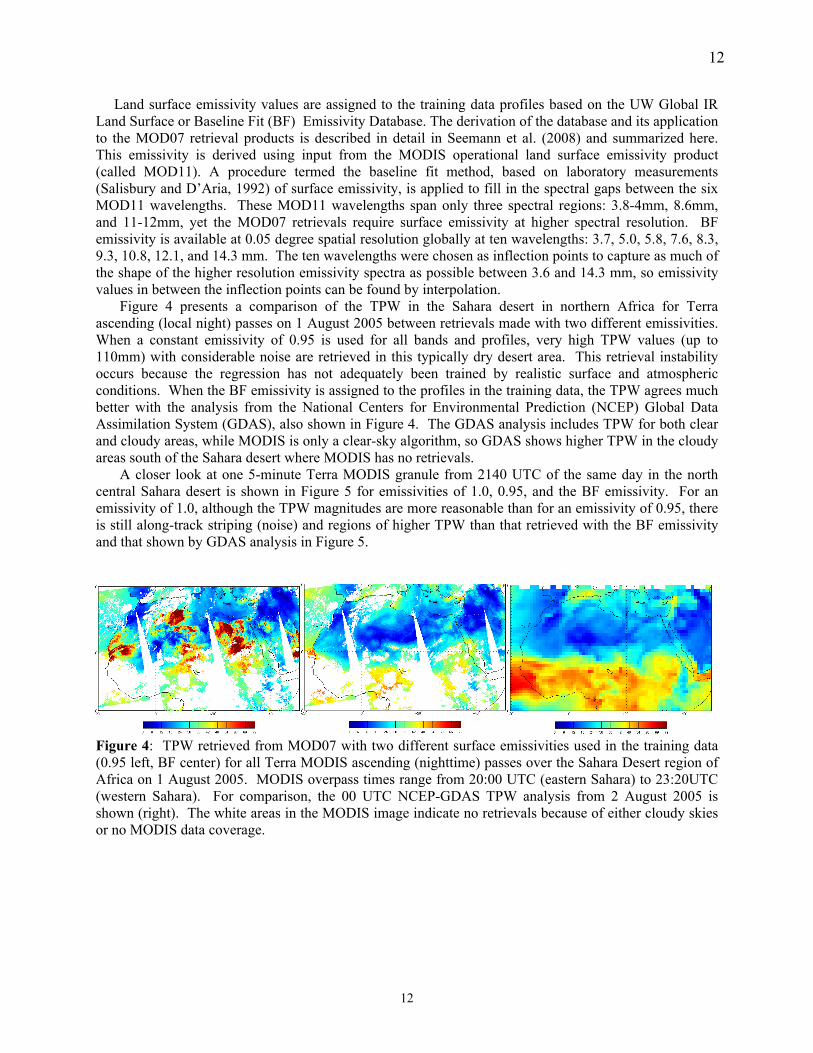
Figure 4 presents a comparison of the TPW in the Sahara desert in northern Africa for Terra ascending (local night) passes on 1 August 2005 between retrievals made with two different emissivities. When a constant emissivity of 0.95 is used for all bands and profiles, very high TPW values (up to 110mm) with considerable noise are retrieved in this typically dry desert area. This retrieval instability occurs because the regression has not adequately been trained by realistic surface and atmospheric conditions. When the BF emissivity is assigned to the profiles in the training data, the TPW agrees much better with the analysis from the National Centers for Environmental Prediction (NCEP) Global Data Assimilation System (GDAS), also shown in Figure 4. The GDAS analysis includes TPW for both clear and cloudy areas, while MODIS is only a clear-sky algorithm, so GDAS shows higher TPW in the cloudy areas south of the Sahara desert where MODIS has no retrievals.

A closer look at one 5-minute Terra MODIS granule from 2140 UTC of the same day in the north central Sahara desert is shown in Figure 5 for emissivities of 1.0, 0.95, and the BF emissivity. For an emissivity of 1.0, although the TPW magnitudes are more reasonable than for an emissivity of 0.95, there is still along-track striping (noise) and regions of higher TPW than that retrieved with the BF emissivity and that shown by GDAS analysis in Figure 5.

Figure 4: TPW retrieved from MOD07 with two different surface emissivities used in the training data (0.95 left, BF center) for all Terra MODIS ascending (nighttime) passes over the Sahara Desert region of Africa on 1 August 2005. MODIS overpass times range from 20:00 UTC (eastern Sahara) to 23:20UTC (western Sahara). For comparison, the 00 UTC NCEP-GDAS TPW analysis from 2 August 2005 is shown (right). The white areas in the MODIS image indicate no retrievals because of either cloudy skies or no MODIS data coverage.

13

13

Figure 5: MODIS MOD07 TPW for the 5 minute Terra granule beginning at 21:40 UTC on August 1, 2005. This granule is in the north-central Sahara desert and is also shown in Figure 4, although the color scale range is different. Emissivities of 0.95 (left), 1.0 (center), and the baseline fit emissivity (right) were applied to the training data used in the regression retrieval algorithm.

4.4.1 Skin Temperature Sensitivity Study

In the MOD07 algorithm, the skin temperature is assigned to training data profiles based on a relationship described in the previous section. This method will be referred as CARTskinT. In this current study, MOD07 TPW derived from various combinations of land surface skin temperature assigned to the MOD07 training profiles were tested. Figures 6 and 7 show the Bias and RMSE, respectively for TPW statistics computed for the SGP ARM site cases (MOD07 vs. SGP microwave radiometer) using various relationships between skin temperature and surface air temperature. The statistics are separated into dry and wet conditions because the algorithm performs quite differently for the two. Table 6 lists the different skin temperature-surface air temperature relationships used in calculating the regression coefficients for the different MOD07 TPW retrievals compared in Figures 6 and 7.

The CARTskinT method has been used in the MOD07 coefficient calculations for a few years and the present study shows that it continues to do well for moist atmospheres, but randomly generated skin temperature performs better for the very dry atmospheric conditions. The conclusions are: 1. Skipping the Antarctic ozonesondes from the training database has no effect on the bias or RMSE for

the dry atmospheric conditions (called dry bias and RMSE later) but does show some improvement for the wet atmospheric conditions (improvement of 0.09mm wet RMSE and 0.06mm wet bias). Also skipping the ECMWF Antarctic profiles does not help (makes things worse).

2. Duplicating the profiles 5 times (5x) in the training database when applying the random skin temperature/surface air temperature difference does not significantly affect the results.

3. Wet bias and wet RMSE are significantly lower for the direct TPW than for the TPW integrated from profiles.

4. Dry bias is significantly higher for the direct TPW, and the dry RMSE is similar but slightly higher for direct TPW.

5. For wet atmospheric conditions, all the cases (see list in Table 6) with CARTskinT have the lowest RMSE; case #4 is the best for both direct (4.17 mm) and integrated TPW (5.26mm). [wet bias of #4 is 4.07mm integrated, and is 2.5mm direct].

6. For dry atmospheric conditions, variations of the random skin T with standard deviation 5, mean 4 (case #8) are the best with both low dry biases (0.0mm integrated, -0.89mm direct) and low dry RMSEs (2.16mm integrated, 2.38 direct). The direct TPW dry biases are always higher.

14

14

Figure 6: TPW Bias (ARM SGP MWR minus MODIS MOD07) in mm for 18 different training data

configurations. The statistics are shown for all cases (All), but also separated into “dry” (TPW < 15 mm) and “wet” (TPW >= 15mm) cases,. The MOD07 TPW product is vertically integrated from the moisture retrievals (no indication in the legend) , but also can be derived directly during the synthetic regression

using as a predictor. The statistics relate to the direct TPW is indicated by “dir” in the legend.

Figure 7 As in Figure 6 except for TPW RMSE (ARM SGP MWR compared with MODIS MOD07) in mm for 18 different training data configurations.

15

15

Table 6 Training data configuration corresponding to case numbers in Figures 6 and 7. CASE NUMBER

TRAINING DATA CONFIGURATION

1 disregard (Old coefficients) 2 disregard (Old coefficients) 3 CART Skin T/Surface Air T diff 4 CART Skin T/Surface Air T diff, no Antarctic ozonesondes 5 CART Skin T/Surface Air T diff, no Antarctic ozonesondes or Antarctic ECMWF

profiles 6 Random Skin T/Surface Air T diff, Standard deviation 5/Mean 4, 5x profiles 7 Random Skin T/Surface Air T diff, Standard deviation 2/Mean 1 8 Random Skin T/Surface Air T diff, Standard deviation 5/Mean 4 9 Random Skin T/Surface Air T diff, Standard deviation 5/Mean 5 10 CART Skin T/Surface Air T diff, ocean Standard deviation 2, mean 0 11 Random Skin T/Surface Air T diff, Standard deviation 1.5/Mean 1 12 Random Skin T/Surface Air T diff, Standard deviation 2.5/Mean 1 13 Random Skin T/Surface Air T diff, Standard deviation 2/Mean 0.5 14 Random Skin T/Surface Air T diff, Standard deviation 2/Mean 1.5 15 Random Skin T/Surface Air T diff, Standard deviation 2/Mean 1 (test 2) 16 Random Skin T/Surface Air T diff, Standard deviation 5/Mean 4 -

EmisFortranTest 17 Same as #16 + old Land Sea Classes 18 Random Skin T/Surface Air T diff, Standard deviation 5/Mean 4 - old Land Sea

Classes

5 Validation of MODIS MOD07 Collection 6 Products Atmospheric retrievals from MODIS have been compared with those from other observing systems to evaluate the algorithm. Comparisons are made with measurements from ground-based instrumentation including the ARM SGP site, the Brewer spectrophotometer located in Budapest, Hungary and the NOAA/FSL (Forecast Systems Laboratory) GPS sites. Retrievals from other satellites are also used for validation, including the GOES sounder moisture and ozone products, AIRS profiles, the Special Sensor Microwave/Imager (SSM/I), Total Ozone Mapping Spectrometer (TOMS) and Ozone Monitoring Instrument (OMI). Some of these comparisons are included in this section.

5.1 Comparison of MODIS TPW with ARM SGP Observations Specialized instrumentation at the ARM SGP site in Oklahoma facilitates comparisons of MODIS atmospheric products with other observations collocated in time and space. The Terra satellite passes over the SGP site daily between 0415-0515 UTC and 1700-1800 UTC. Radiosondes are launched three times each day at approximately 0530, 1730, and 2330 UTC. Observations of total column moisture are made by the microwave water radiometer (MWR) every 40-60 seconds. An additional comparison is possible with the GOES-8 Sounder which retrieves TPW hourly. Based on manual inspection of radiance images to screen for cloudy cases, a database of clear sky cases at the ARM SGP site has been developed for evaluating the MOD07 total precipitable water (TPW) product. This database includes all overpasses determined to be clear during the period from launch

16

16

through August 2005 for a total of 345 Terra and 317 Aqua cases. MODIS sensor zenith angle was less than 50o to the Lamont, OK SGP site for all cases. These cases can all be reprocessed in-house easily to test any changes to the algorithm or training data. MOD07 TPW is compared with the ARM microwave water radiometer (MWR), radiosonde, and TPW from the GOES satellite for all cases. The comparison for both Terra and Aqua is shown in Figure 8. Both the original and direct TPW are compared. MOD07 “direct” TPW is retrieved using TPW as a predictor. For the original TPW, moisture profiles are retrieved and integrated. Both variables are saved in the operational MOD07 files. RMSE for Terra and Aqua, compared to the MWR is 2.9 mm, with an overall bias near zero. Statistics for both Aqua and Terra compared with the MWR, separated into dry and moist cases, are shown in Table 7.

Figure 8: Comparison of total precipitable water (mm) at the ARM SGP site from MODIS (y-axis, red dots original, green dots “direct”): Aqua (left) and Terra (right) with the MWR. Also compared with the MWR are GOES-8 and -12 (blue diamonds) and radiosonde (black x’s). 317 Aqua and 345 Terra manually-selected clear sky cases from launch through 8/2005 are compared using the Collection 6 MODIS MOD07 algorithm.

5.1.1 Effect of the H2O/CO2 Channel Spectral Shifts on the MODIS TPW MOD07 TPW values were derived with and without applying the Aqua H2O/CO2 channel spectral shifts, and then they were compared with the MWR, radiosonde, and TPW from the GOES satellite for all cases over the SGP ARM Cart Site. Table 7 and Figures 9 and 10 show the results.

Over the SGP cart site when using the CRTM model for the forward calculation, the application of Aqua spectral shifts shows significant improvement particularly in the wet cases (TPW > 15mm) where the rms error was improved by 1.9 mm and the bias was reduced by 2.3 mm. The SRF shifts reduced the big dry bias – found previously in the Collection 5 TPW product (see Aqua Col 5.2 line in Table 1) - in the wet cases by adding more moisture into the atmosphere. After the spectral shifts were applied on the Aqua MODIS instrument, the statistics look very similar to those for the Terra satellite data without the shifts. The cases (highlighted with yellow in Table 7) were selected for the new Collection 6 algorithm. Figure 9 illustrates the bias dependence by the water vapor content, where applying the H20/C02 channel SRF shifts gradually reduced the biases. Figure 10 shows a sample granule for Aqua MODIS with the effects of applying and not applying the spectral shifts compared to the GOES TPW field. The added moisture by the SRF shifts is obvious over the wettest area.

For the Terra cases the new Collection 6 products may look slightly worse, but we should keep in mind that we want to use the same MOD07 Collection 6 algorithm for both satellite because it uses the

17

17

most up-to-date forward model without the bias adjustment which was previously specifically developed over one location (the SGP cart site). There are no spectral shifts applied for Col 6 Terra/MODIS, but in the future we are planning to apply the Terra channel SRF shifts indicated by Quinn et al (2010, 2011).

Table 7: TPW comparison at the ARM SGP site between MWR and MOD07 TPW for 317 Aqua (top table) and 345 Terra (middle table) clear sky cases from Sept 2002 to August 2005. Dry and wet cases are also separated and shown. The version of the MOD07 algorithm is listed in the first column and the use of H2O/CO2 channel SRF shifts is indicated in the second column. The number of cases involved in the statistics is located in the parentheses. Bias and rms differences between GOES and Radiosondes and MWR are also included for reference at the bottom of the table.

MOD07 versions

SRF shift

DRY (TPW<15mm) (228) Bias RMS

WET (TPW >=15mm) (89) Bias RMS

ALL (317 cases) Bias RMS

Aqua Col 5.2 No -0.4 2.2 3.6 5.1 0.8 3.3 Aqua Col 6 No -0.2 2.3 4.6 5.7 1.1 3.6 Aqua Col 6 Yes -0.8 2.5 2.3 3.8 0.1 3.0

MOD07 versions

SRF shift

DRY (TPW<15mm) (217) Bias RMS

WET (TPW >=15mm) (128) Bias RMW

ALL (345 cases) Bias RMS

Terra Col 5.2 No -0.7 2.0 1.1 3.2 -0.04 2.5 Terra Col 6 No -0.7 2.0 1.9 4.0 0.3 2.9

Bias RMS

GOES -0.1 2.0 (171) Radisonde 0.6 1.3 (282)

Figure 9: TPW differences between MWR and MOD07 data (y-axis) vs. the MWR TPW (X-axis) at the ARM SGP site for 317 clear sky cases from Sept 2002 to August 2005. Red stands for the Collection 6 algorithm run without the SRF shift applied and blue indicates the run with the spectral shift application.

18

18

Figure 10: Total Precipitable Water field from July 3, 2003, at 08:00 UTC.

5.2 Comparison of MOD07 Total Ozone with Brewer instrument The MODIS “total_ozone” amount (TOZ) has been evaluated in Central Europe using surface Brewer measurements as the most accurate measurements of the vertically integrated ozone values. These data were measured with the Brewer spectrophotometer located in Budapest (as the 152nd member of the Brewer Network) and were provided by the Hungarian Meteorological Service. The values of the surface observations were temporally interpolated for the time of the overpasses of Terra and Aqua based on the data measured by the Brewer instrument every 15-25 minutes. (Most of measurements were retrieved from the direct radiation of the Sun; however when the sun-disk was covered by clouds, the calculation was based on zenith observations.) For the comparison of the two total ozone estimations retrieved from remote sensing data with the surface observations, we always selected the closest pixel from the actual irregular MODIS grid to the coordinates of the Brewer instrument located in Budapest.

The MODIS data were received by the polar orbiting satellite receiving station at Eötvös Loránd University, in Budapest, Hungary (47.475°N, 19.062°E) and processed by the IMAPP software. The comparisons were performed using MODIS data from selected overpasses for the year 2007: specifically, 102 and 41 overpasses of Terra and Aqua, respectively, which were mostly cloudfree in the vicinity of Budapest, and in the Carpathian-Basin.

In our comparison study, the daily, 1°×1° horizontal grid resolution OMI total ozone data (http://toms.gsfc.nasa.gov) are also included. The OMI total ozone data were remapped to the MODIS observations by using bilinear interpolation. The resulting remapped image (see Figure 13) preserves its original structure and can be applied for the comparison without restrictions. Table 8 summarizes the statistics of the TOZ comparison between the OMI and MOD07, and the surface Brewer measurements. The table shows that the OMI agrees the most with Brewer measurements with a correlation larger that 0.96. The new MOD07 collection 6 algorithm with the Aqua H2O/CO2 channel spectral shifts applied results in the best correlation (the lowest standard deviation) with the Brewer measurements among the MODIS Col 5.2 and Col 6 with and without the shifts applied. The correlation (and stdev) for Terra/MODIS TOZ is also improved by the new algorithm. In the future, the larger Terra/MODIS bias (see also Figure 11 and 12) should be reduced by the application of Terra H2O/O3 channel spectral shifts. The year-long time series of TOZ observations in Figure 11 shows the smaller Aqua scattering and indicates that MODIS follows nicely the annual trend by OMI, the ECMWF ERA40, and Brewer Total Ozone.

19

19

Table 8: Comparison of TOZ measured by OMI and MODIS (Terra and Aqua) vs the surface Brewer measurements for year 2007 over Budapest, Hungary. Bias, standard deviation, root mean square error and correlation are included.

Satellite-based TOZ vs. Surface Brewer Measurements

Bias [DU] Stdev [DU] RMSE [DU] R2

OMI at Terra overpass times 6.8 6.9 9.7 0.96

MOD07/Terra Col 5.2 -16.8 20.0 26.1 0.69

MOD07/Terra Col 6 without spectral shifts -26.5 17.3 31.6 0.76

OMI at Aqua overpass times 0.6 7.5 7.6 0.99

MYD07/Aqua Collection 5.2 6.0 20.8 21.6 0.81

MYD07/Aqua Col 6 without spectral shifts -1.2 17.6 17.7 0.83

MYD07/Aqua Col 6 with spectral shifts 4.0 16.0 16.5 0.88

Figure 11: Scatter plot of satellite-based (MODIS and OMI) Total Ozone vs. ground-based Brewer measurements for the year 2007 at Budapest, Hungary.

20

20

Figure 12: Time series of Total Ozone observations for the year 2007 over Budapest, Hungary separated by Aqua and Terra overpass times. The ECMWF ERA40 daily mean and absolute maximum and minimum TPW for the year 2007 are also plotted in grey.

Figure 13: Total Ozone by Aqua/MODIS (left) and OMI (right) on July 8, 2007 at 12:18:55 UTC.

21

21

5.3 Global evaluation of MOD07 Total Ozone The MOD07 “Total_Ozone” (TOZ) product is routinely compared with the Total Ozone Mapping Spectrometer (TOMS; McPeters et al. 1998, 1996; Bowman and Krueger, 1985) ozone and AIRS atmospheric retrievals on a global scale for different seasons.

In Table 9 the MODIS Total Ozone retrievals derived by the Collection 5 and the new Collection 6 MOD07 algorithm were compared globally against TOMS and AIRS products. Three days of Aqua MODIS data (12.01.2004, 08.28.2006, and 02.01.2007) and three days of Terra MODIS data (08.14.2001, 03.11.2006, and 08.28.2006) were chosen for study. The TOMS measurements are from the Earth Probe platform (Version 8 products) or the OMI platform (Version 3 products) depending on the study date. For the TOMS ozone comparisons, MODIS total ozone was averaged onto the Level 3 TOMS grid of 1.25-degree longitude by 1.00-degree latitude. For the AIRS comparison, Version 5 Level 2 standard retrieval AIRS products (AIRSX2RET) are used. In these comparisons, both the AIRS products and the MODIS products were averaged onto a common grid of 0.5-degree latitude by 1.0-degree longitude. Maps of the number of points, standard deviations, RMS, averages and differences within each grid bin were produced. The global mean differences and standard deviations for TOZ are summarized in Table 9. The highest one third of the standard deviations and values above 70 degrees latitude have been removed from the comparison. Table 9: Global comparison of MOD07 Total Ozone (Dobson Unit) with OME TOMS and AIRS retrievals for three selected days. Biases and standard deviations for Aqua (top panel) and Terra (bottom panel) are shown. MODIS TOZ without and with the spectral shifts are also calculated and shown for the three days.

Date (Aqua) TOZ [DU] OMI-MYD07 (Col5)

bias ± Stdev

OMI– MYD07 (Col6)

Bias ± Stdev

AIRS–MYD07 (Col5)

Land Sea

AIRS–MYD07 (Col6)

Land Sea

Dec 1 2004 / with no shifts +24±27 +8±22 +34±41 +21±25 +20±37 +8±19

with shifts - +19±21 - - +29±36 +19±20

Aug 28 2006 with no shifts +16±24 +0±27 +29±23 +19±20 +8±21 +5±19

with shifts - +13±25 - - +18±26 +19±19

Feb 1 2007 / with no shifts +12±23 -3±30 +18±38 +14±24 -2±40 +3±21

with shifts - +7±29 - - +7±42 +14±24

Date (Terra) TOZ [DU] No shifts

OMI–MOD07 (Col5) bias ± Stdev

OMI –MOD07 (Col6) Bias ± Stdev

AIRS–MOD07 (Col5) Land Sea

AIRS–MOD07 (Col6) Land Sea

Aug 14 2001 +2±17 -9±26 - - - -

March 11 2006 -1±29 -14±49 +7±38 -1±19 +27±52 -5±34

Aug 28 2006 / +1±25 -8±41 -+29±71 +9±66 -0.6±38 -3±30

22

22

Global comparisons of total column ozone with TOMS and MOD07 show agreement to within 20 D.U. (6%) with a standard deviation of 30 D.U. (9%) assuming an average of ~350 D.U. The Aqua bias for Collection 6 is an improvement over Collection 5, but the standard deviations have not changed appreciably. Using the new forward model helped mostly to reduce the biases compared to both OMI TOMS and AIRS values, the positive effect of the H2O/CO2 spectral shifts on TOZ is not as obvious as it was shown on the local comparison in Section 3.2. In the future the Aqua O3 channel spectral shift will be investigated. The improvements for Terra/MODIS are assumed after applying the Terra spectral shifts in the future. Generally for both satellites, the bias and standard deviations over ocean are smaller than over land.

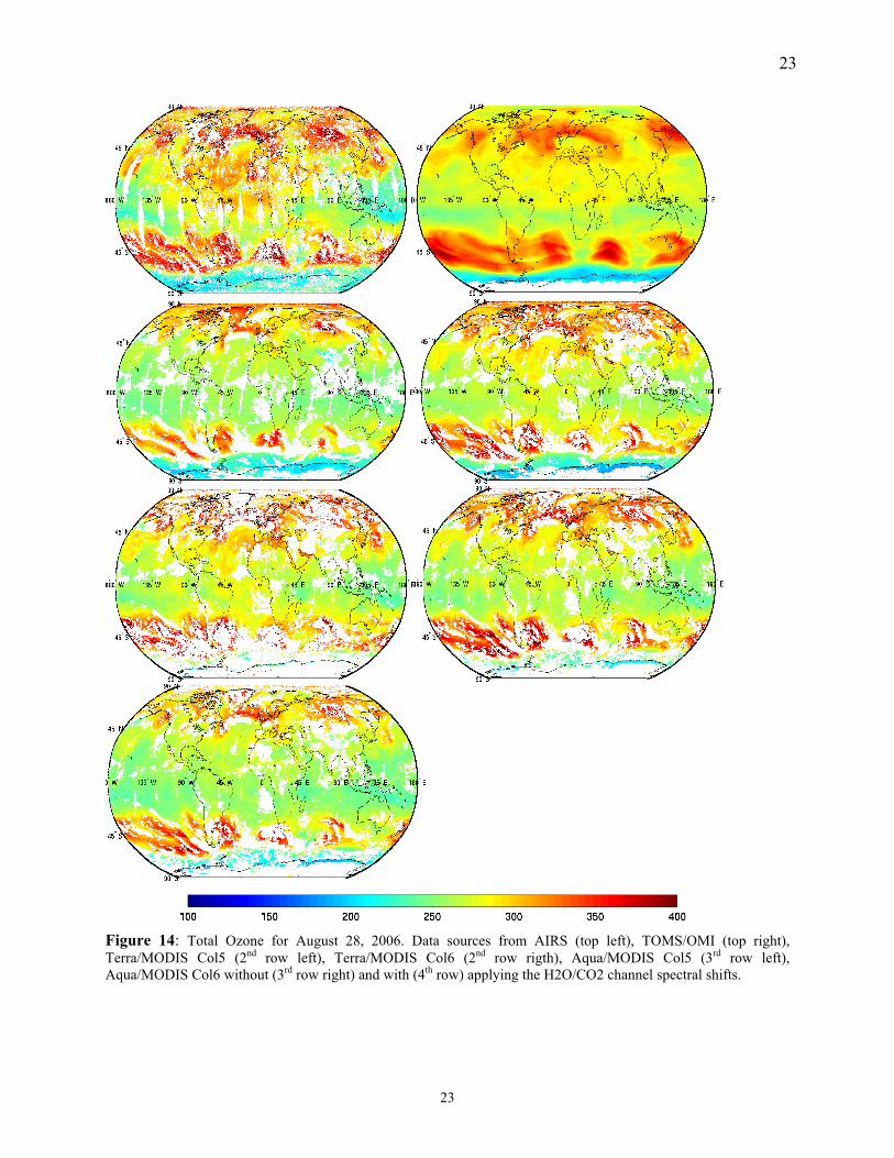
One example is shown in Figure 14, a summer case (August 28, 2006) showing elevated ozone in the northern hemisphere and lower in the southern hemisphere. General features in the TOMS ozone are also captured by the MODIS ozone.

5.4 Global Evaluation of MOD07 TPW We routinely use the SGP ARM CART site clear sky dataset (over 300 cases) as a validation tool for MOD07 TPW products (see section 3.1). To determine the quality of our products over other places, especially over oceans, a global intercomparison of TPW was performed for a couple of select days for both Terra and Aqua satellites. The MODIS TPW (‘Water_Vapor’) products were compared with the AIRS operational products (totH2OStd).

The AIRS Level2 ‘totH2OStd’ variable was used for the global TPW validation study. Values were averaged onto a 360x360 grid (0.5o lat x 1.0 o long) and the ‘landFrac’ variable was used to determine land (> 0.9) or sea (<=0.1) pixel location. The MODIS Collection 5 and Collection 6 ‘Water_Vapor’ variables were averaged onto the same grid, and the ‘Cloud_Mask.landWater’ products were used to separate the land/sea cases (>0 are land, 0 is ocean). Table 10 summarizes the bias and standard deviation differences in TPW between AIRS and MODIS Collections 5 and 6 (AIRS-MODIS) for the selected cases separated by scene. The results show that MODIS Collection 6 TPW values agree well with the AIRS products. The bias is within ±2.3mm (9 %) and the standard deviation is less than 6.5 mm (25 %) out of an average of ~ 25 mm (Amenu and Kumar, 2005) in most cases. Biases over land were reduced by more than 1 mm, which means that MODIS became wetter than the AIRS TPW. Since the global comparison shows no significant differences between the Collection 5 and 6 products, in the future further investigation is necessary to classify the comparisons for wet/dry cases and study the quality of the AIRS TPW products themselves.

Figure 15 shows an example of the AIRS and MODIS TPW global map for a selected day (2004336). The figure also shows that the application of the Aqua spectral shifts in the Collection 6 algorithm added more moisture in the wetter tropical area.

23

23

Figure 14: Total Ozone for August 28, 2006. Data sources from AIRS (top left), TOMS/OMI (top right), Terra/MODIS Col5 (2nd row left), Terra/MODIS Col6 (2nd row rigth), Aqua/MODIS Col5 (3rd row left), Aqua/MODIS Col6 without (3rd row right) and with (4th row) applying the H2O/CO2 channel spectral shifts.

24

24

Table 10: Bias and standard deviation differences between MODIS MOD07/MYD07 TPW and AIRS L2 operational TPW products separated by scene (sea/land) for the following global days: Dec 1 2004 (2004336), Aug 28 2006 (2006240), Feb 1 2007 (2007032), Aug 14 2001 (2001226), and March 11 2007 (2006070).

Date (Aqua) TPW[mm]

AIRS–MYD07(Col5) Land Sea

AIRS–MYD07(Col6) Land Sea

Dec 1 2004 +0.6±5.0 -1.8±5.2 -0.9±5.7 -0.8±4.6

Aug 28 2006 -0.6±5.7 -1.3±4.3 -2.3±6.5 -1.3±4.7

Feb 1 2007 0.0±4.1 -1.3±5.1 -0.9±5.8 -1.5±4.8

Figure 15: Comparison of the official AIRS L2 (top left) standard TPW products and MODIS Collection 5 (top right) and Collection 6 TPW products with spectral shifts applied (top right) and without for December 1, 2004.

6 Technical Issues The MODIS temperature and moisture profile retrieval algorithm is dependent on the quality of the MODIS Level-1B data provided as input. While instrument noise is important, other factors that affect the quality of retrievals are noisy and/or dead detectors; detector imbalances; mirror side characterization; response vs. scan angle, and spectral shifts. Many of these effects are difficult to characterize and correct, and such corrections are beyond the scope of the temperature and moisture profile retrieval algorithm.

6.1 Destriping of Input MODIS Radiances To address across track striping present in the MOD07 retrievals as a result of detector-to-detector differences in radiances, input MODIS L1B 1KM radiances are destriped prior to performing retrievals

25

25

operationally. The MODIS destriping algorithm is based on the method of Weinreb et al. (1989). The algorithm accounts for both detector-to-detector and mirror side striping. MODIS is treated as a 20 detector instrument in the emissive bands (10 detectors on each mirror side). The empirical distribution function (EDF) is computed for each detector (cumulative histogram of relative frequency). The EDF for each detector is adjusted to match the EDF of a reference in-family detector. The algorithm operates on L1B scaled integers (0-32767). The median scaled integer value is restored following destriping. Correction LUT is created for each individual granule. Uncorrected scaled integers are replaced with corrected scaled integers (could store the correction LUT instead). Bands 20, 22-25, 27-30, 33-36 are destriped. Impact on bands 31 and 32 is equivocal. For Terra MODIS, noisy detectors in some bands are replaced with neighbors: 27 (dets 0, 6); 28 (dets 0, 1); 33 (det 1); 34 (dets 6, 7, 8) . For Aqua MODIS, one detector in band 27 is replaced.

6.2 Instrument Errors A complete error analysis including the effects of instrument calibration and noise as well as ancillary input data errors remains to be completed. The past performance of these algorithms with HIRS data is documented as temperature profiles errors at about 1.9 C, dewpoint temperature profile errors at about 4 C, total column ozone at about 10%, total column water vapor at about 10%, and gradients in atmospheric stability within 0.5 C. The profile and total atmospheric column algorithms are based on HIRS experience. One significant difference between MODIS and HIRS is the absence of any stratospheric channels on MODIS (15.0, 14.7, and 14.5 mm). This primarily affects the accuracy of the total ozone concentration estimates. The assumption for the MODIS algorithms presented here is that the slowly varying stratospheric temperatures are estimated very well by the forecast model.

6.3 Data Processing Considerations Processing is accomplished globally at 5´5 pixel resolution in regions where a sufficient number of clear FOVs are available. Radiances within the clear FOVs are averaged to reduce instrument single sample noise. The algorithm checks the validity of all input radiances, and if the required input radiance data are bad, suspect, or not available, then the algorithm will record the output products as missing for that 5´5 pixel area. Thus, regarding to the MOD07 retrievals products quality assurance, there are either have sufficient data (e.g. at least 5 out of 25 pixels defined as confident clear) and the "Best Quality Data" retrievals are produced or the retrievals are flagged missing. The MOD07 retrievals are thus considered to be best quality. The MODIS Cloud Mask is used for cloud screening and for surface type determination (land or sea). The NCEP GDAS1 6-hourly global analysis estimates of surface pressure at 1 degree resolution are the only non-MODIS ancillary input required for the algorithm.

6.4 Quality Control Automatic tests in the code check for physically realistic output values of temperature and moisture. In addition, daily, 8-day, and monthly composites of primary output products such as temperatures at 300, 500, and 700 hPa pressure levels; total precipitable water vapor, and total ozone are routinely monitored for consistency via the MODIS Atmosphere Group website at http://modis-atmos.gsfc.nasa.gov/ .

26

26

6.5 Output Product Description MOD07_L2 product files are stored in Hierarchical Data Format (HDF). HDF is a multi-object file format for sharing scientific data in multi-platform distributed environments. HDF files should only be accessed through HDF library subroutine and function calls, which can be downloaded from the http://hdf.ncsa.uiuc.edu website. Each gridded parameters listed belowis stored as a Scientific Data Set (SDS) within the HDF file. The values stored in the SDS (other then the geolocation arrays) are short integer values in order to save storage space. To calculate the real data value, the scale_factor and the add_offset are needed to apply to the stored value. These are local attributes attached to each SDS. The following equation should be used to get to the real value: Value = scale_factor*(stored_value-add_offset) .

A single output file (MOD07) combining four products will be generated as part of the MODIS atmospheric profile retrieval algorithm; Table 11 lists the parameters and their units.

Table 11: Parameters included in products MOD30, MOD07, MOD38, MOD08 Resolution: 5 × 5 pixel, Temporal sampling: Day and Night, Restrictions: Clear Sky only TAI time at start of scan (seconds since 1993-1-1 00:00:00.0 0) Geodetic Latitude (degrees_north) Geodetic Longitude (degrees_east) Solar Zenith Angle, Cell to Sun (degrees) Solar Azimuth Angle, Cell to Sun (degrees) Sensor Zenith Angle, Cell to Sensor (degrees) Sensor Azimuth Angle, Cell to Sensor (degrees) Brightness Temperature, IR Bands (K) Cloud Mask, First Byte (no units) Surface Skin Temperature (K) Surface Pressure (hPa) Processing Flag (no units) Tropopause Height (hPa) Guess Temperature Profile (K) Guess Dew Point Temperature Profile (K) Retrieved Temperature Profile (K) Retrieved Dew Point Temperature Profile (K) Retrieved Mixing Ratio Profile (g/kg) Total Ozone Burden (Dobsons) Total Totals Index (K) Lifted Index (K) K Index (K) Total Column Precipitable Water Vapor, IR (cm) Precipitable Water Vapor Low, IR (cm) Precipitable Water Vapor High, IR (cm) Retrieval Profile Pressure Levels (hPa) 5, 10, 20, 30, 50, 70, 100, 150, 200, 250, 300, 400, 500, 620, 700, 780, 850, 920, 950, 1000

27

27

7 Summary of the MODIS MOD07 algorithm updates for Collection 6:

•Updated the radiative transfer model to CRTM V1.2 (from the prototype CRTM). •Applied the zero bias adjustment in the radiative transfer calculation. •Applied H2O/CO2 channel spectral shifts for Aqua (Tobin et al., 2006, JGR). •Updated NedT for both Terra and Aqua. •In the training database the surface emissivity spectra were updated to the current version. •Made the Aqua and Terra DAAC code uniform. •Modified the TPW Low and TPW high products to be able to calculate three layer water vapor means. The new layers are: (Low) sfc-680 and (high) 440-top (10hPa). •Improve QA/QC flags, QA usefulness and Confidence flag bug is fixed. •Output file updates: added offset/scale factor usage, list of pressure levels, K-index valid range fixed, surface temperature changed to skin temperature, mixing ration profile added. •The new products were tested over the SGP ARM cart site with MWR and GOES, over Budapest, Hungary with Brewer and TOMS/OMI measurements, and over some select global days with TOMS and AIRS data.

8 Future work Future work planned for the MOD07 algorithm is listed below:

1. Continue monitoring the algorithm, making adjustments as appropriate (due to the change in the atmospheric training dataset, the radiative transfer model etc.)

2. Continue the regional and global validation of MODIS atmospheric profile products with MWR, RAOB, GOES, TOMS, AIRS and SSM/I.

3. Study the Aqua spectral shifted SRF of the ozone band (31) and its effect on the Total Ozone Product.

4. Study the possibility of spectral shifted SRF of the IR bands on Terra. 5. Investigate the atmospheric profile products at one kilometer resolution 6. Conduct TPW comparisons at 1km and 5 km various resolution 7. Investigate the improve QA/QC flags and screening for bad input MOD02L1B data specially in

the case on 1 km resolution processing mode. 8. Save MOD07 retrieved infrared land surface emissivity retrievals to operational output files.

Currently emissivity is retrieved but only saved for one wavelength.

28

28

9 Acknowledgements: We thank the Hungarian Meteorological Service and Zoltan Toth for providing and processing the surface Brewer Spectrophotometer measurements for validating the MOD07 Total Ozone product.

10 References Ackerman, S. A., K. I. Strabala, W. P. Menzel, R. A. Frey, C. C. Moeller, and L. E. Gumley, 1998:

Discriminating clear sky from clouds with MODIS. J. Geophys. Res., 103, D24, 32141-32157. ____, R. E. Holz, R. A. Frey, E. W. Eloranta, B. C. Maddux, and M. McGill, 2008: Cloud detection with

MODIS. Part II: validation. Journal of Atmospheric and Oceanic Technology, Volume 25, 1073-1086.

Amenu, G.G., and P. Kumar, 2005: NVAP and Reanalyses-2 Global Precipitable Water Products: Intercomparison and variablility Studies. BAMS, February, 2005.

Borbas, E., S. W. Seemann, H.-L. Huang, J. Li, and W. P. Menzel, 2005: Global profile training database for satellite regression retrievals with estimates of skin temperature and emissivity. Proc. of the Int. ATOVS Study Conference-XIV, Beijing, China, 25-31 May 2005, pp763-770.

Bowman, K.P. and A.J. Krueger, 1985: A global climatology of total ozone from the Nimbus-7 Total Ozone Mapping Spectrometer", J. Geophys. Res., 90, 7967-7976.

Eyre, J. R., and H. M. Woolf, 1992: A bias correction scheme for simulated TOVS brightness temperatures. ECMWF Technical Memorandum 186. 28 pp.

Fleming, H. E. and W. L. Smith, 1971: Inversion techniques for remote sensing of atmospheric temperature profiles. Reprint from Fifth Symposium on Temperature. Instrument Society of America, 400 Stanwix Street, Pittsburgh, Pennsylvania, 2239-2250.

Fritz, S., D. Q. Wark, H. E. Fleming, W. L. Smith, H. Jacobowitz, D. T. Hilleary, and J. C. Alishouse, 1972: Temperature sounding from satellites. NOAA Technical Report NESS 59. U.S. Department of Commerce, National Oceanic and Atmospheric Administration, National Environmental Satellite Service, Washington, D.C., 49 pp.

Han, Y., P. Delst, Q. Liu, F. weng, B. Yan, and J. Derber, 2005: User’s Guide to the JCSDA Community Radiative Transfer Model (Beta Version), http://www.star.nesdis.noaa.gov/smcd/spb/CRTM/crtm-code/CRTM_UserGuide-beta.pdf.

Harris, B. A., and G. Kelly, 2001: A satellite radiance bias correction scheme for radiance assimilation. Quart. J. Roy. Meteor. Soc., 127, 1453-1468.

Hayden, C. M., 1988: GOES-VAS simultaneous temperature-moisture retrieval algorithm. J. Appl. Meteor., 27, 705-733.

Houghton, J. T., Taylor, F. W., and C. D. Rodgers, 1984: Remote Sounding of Atmospheres. Cambridge University Press, Cambridge UK, 343 pp.

Huang, H.-L. et al., 2004: International MODIS and AIRS Processing Package (IMAPP): A direct broadcast software package for the NASA Earth Observing System. Bull. Of the American Met. Soc., 85, No.2, 159-161.

Kaplan, L. D., 1959: Inference of atmospheric structure from remote radiation measurements. Journal of the Optical Society of America, 49, 1004.

King, J. I. F., 1956: The radiative heat transfer of planet earth. Scientific Use of Earth Satellites, University of Michigan Press, Ann Arbor, Michigan, 133-136.

King, M.D., Kaufman, Y. J., Menzel, W. P. and D. Tanré, 1992: Remote sensing of cloud, aerosol, and water vapor properties from the Moderate Resolution Imaging Spectrometer

Kleespies, T. J., P. van Delst, L. M. McMillin, and J. Derber, 2004: Atmospheric Transmittance

29

29

of an Absorbing Gas. 6. OPTRAN Status Report and Introduction to the NESDIS/NCEP Community Radiative Transfer Model. Appl. Opt., 43, 3103-3109.

Li, J., and H.-L. Huang, 1999: Retrieval of atmospheric profiles from satellite sounder measurements by use of the discrepancy principle, Appl. Optics, Vol. 38, No. 6, 916-923.

Li, J., W. Wolf, W. P. Menzel, W. Zhang, H.-L. Huang, and T. H. Achtor, 2000: Global soundings of the atmosphere from ATOVS measurements: The algorithm and validation, J. Appl. Meteorol., 39: 1248 – 1268.

Ma, X. L., Schmit, T. J. and W. L. Smith, 1999: A non-linear physical retrieval algorithm – its application to the GOES-8/9 sounder. Accepted by J. Appl. Meteor.

McPeters, R.D, Krueger, A.J., Bhartia, P.K., Herman, J.R. et al, 1996: Nimbus-7 Total Ozone Mapping Spectrometer (TOMS) Data ProductsUser's Guide, NASA Reference Publication 1384, available from NASA Center for AeroSpace Information, 800 Elkridge Landing Rd, Linthicum Heights, MD 21090, USA; (301) 621-0390.

McPeters, R.D, Krueger, A.J., Bhartia, P.K., Herman, J.R. et al, 1998: Earth Probe Total Ozone Mapping Spectrometer (TOMS) Data ProductsUser's Guide, NASA Reference Publication 1998-206895 , available from NASA Center for AeroSpace Information, 800 Elkridge Landing Rd, Linthicum Heights, MD 21090, USA; (301) 621-0390.

Menzel, W. P., and J. F. W. Purdom, 1994: Introducing GOES-I: The first of a new generation of geostationary operational environmental satellites. Bull. Amer. Meteor. Soc., 75, 757-781.

Menzel, W. P., F. C. Holt, T. J. Schmit, R. M. Aune, A. J. Schreiner, G. S. Wade, and D. G. Gray, 1998. Application of the GOES-8/9 soundings to weather forecasting and nowcasting. Bull. Amer. Meteor. Soc., 79, 2059-2077.

Quinn et al, 2010, http://www.ssec.wisc.edu/~gregq/iasi-modis/plots.html ____, G., R.W. Holz, F.W. Nagle, W. Wolf and H. Sun: Developing a product validation and inter-

calibration system for GOES-R using advanced collocation methods, 91th AMS Annual Meeting, Jan 2011. http://ams.confex.com/ams/91Annual/webprogram/Paper187296.html

Rodgers, C. D., 1976: Retrieval of atmospheric temperature and composition from remote measurements of thermal radiation. Rev. Geophys. Space Phys., 14, 609-624.

Salisbury, J.W., and D.M. D’Aria, 1992: Emissivity of terrestrial materials in the 8-14mm atmospheric window. Remote Sensing of the Environment, 42, 83-106.

Schmit, T. J., Feltz, W. F., Menzel, W. P., Jung, J., Noel, A. P., Heil, J. N., Nelson, J. P., and G.S.Wade, 2002: Validation and Use of GOES Sounder Moisture Information. Wea. Forecasting, 17, 139-154.

Seemann, S. W., J. Li, W. P. Menzel, and L. E. Gumley, 2003. Operational retrieval of atmospheric temperature, moisture, and ozone from MODIS infrared radiances. J. Appl. Meteor., 42, 1072-1091.

____, Borbas, E.E., Knuteson, R.O., Stephenson, G.R., and Huang, H-L., 2008: Development of a global infrared emissivity database for application to clear sky sounding retrievals from multi-spectral satellite radiances measurements. J. Appl. Meteorol. and Clim. 47, 108-123 Smith, W. L., Woolf, H. M., and W. J. Jacob, 1970: A regression method for obtaining real-time

temperature and geopotential height profiles from satellite spectrometer measurements and its application to Nimbus 3 “SIRS” observations. Mon. Wea. Rev.., 8, 582-603.

____, Woolf, H. M., Hayden, C. M., Wark, D. Q. and L. M. McMillin, 1979: The TIROS-N operational vertical sounder. Bull. Amer. Meteor. Soc., 60, 1177-1187.

____, Suomi, V. E., Menzel, W. P., Woolf, H. M., Sromovsky, L. A., Revercomb, H. E., Hayden, C. M., Erickson, D. N. and F. R. Mosher, 1981: First sounding results from VAS-D. Bull. Amer. Meteor. Soc., 62, 232-236.

____, and F. X. Zhou, 1982: Rapid extraction of layer relative humidity, geopotential thickness, and atmospheric stability from satellite sounding radiometer data. Appl. Opt., 21, 924-928.

____, and H. M. Woolf, 1988: A Linear Simultaneous Solution for Temperature and Absorbing Constituent Profiles from Radiance Spectra. Technical Proceedings of the Fourth International TOVS Study Conference held in Igls, Austria 16 to 22 March 1988, W. P. Menzel Ed., 330-347.

30

30

____, 1991: Atmospheric soundings from satellites - false expectation or the key to improved weather prediction. Jour. Roy. Meteor. Soc., 117, 267-297.

____, Woolf, H. M., Nieman, S. J., and T. H. Achtor, 1993: ITPP-5 - The use of AVHRR and TIGR in TOVS Data Processing. Technical Proceedings of the Seventh International TOVS Study Conference held in Igls, Austria 10 to 16 February 1993, J. R. Eyre Ed., 443-453.

Tobin, D. C., H. E. Revercomb, R. O. Knuteson, B. M. Lesht, L. L. Strow, S. E. Hannon, W. F. Feltz, L. A. Moy, E. J. Fetzer, and T. S. Cress 2006: Atmospheric Radiation Measurement site atmospheric state best estimates for Atmospheric Infrared Sounder temperature and water vapor retrieval validation, J. Geophys. Res., 111, D09S14, doi:10.1029/2005JD006103.

____, D. C.; Revercomb, Henry E.; Moeller, Christopher C. and Pagano, Thomas S. 2006: Use of Atmospheric Infrared Sounder high-spectral resolution spectra to assess the calibration to Moderate resolution Imaging Spectroradiometer on EOS Aqua. Journal of Geophysical Research, Volume 111, 2006, Doi:10.1029/2005JD006095, 2006. Call Number: Reprint # 5053. http://www.agu.org/pubs/crossref/2006/2005JD006095.shtml

Twomey, S., 1977: An introduction to the mathematics of inversion in remote sensing and indirect measurements. Elsevier, New York.

Wark, D. Q., 1961: On indirect temperature soundings of the stratosphere from satellites. J. Geophys. Res., 66, 77.

____, Hilleary, D.T., Anderson, S. P., and J. C. Fisher, 1970: Nimbus satellite infrared spectrometer experiments. IEEE. Trans. Geosci. Electron., GE-8, 264-270.

Weinreb et al., 1989: Destriping GOES Images by Matching Empirical Distribution Functions. Remote Sens. Environ., 29, 185-195.