module 14 solutions

Module 14

Cost Behavior, Activity Analysis, and Cost Estimation

DISCUSSION QUESTIONS

Q14-1. Variable, fixed, mixed, and step costs and their related total cost functions are described as follows:

Variable costs are uniform for each incremental unit of activity. Total variable costs change in direct proportion to changes in activity, equaling zero dollars when activity is zero and increasing at a constant amount per unit of activity.

Fixed costs are a constant amount per period of time. The fixed cost curve is flat with a slope of zero.

Mixed costs contain a fixed and a variable cost element. They are positive when activity is zero and increase in a linear fashion as activity increases.

Step costs are constant within a given range of activity but differ between ranges of activity. They increase in a step-like fashion as activity increases.

Q14-2. Because of the multitude of underlying factors that drive costs, presenting all costs of an organization as a function of a single independent variable is not accurate enough to make specific decisions concerning products, services, or activities.

©Cambridge Business Publishers, 2013

Solutions Manual, Module 14 14-1

Q14-3. The vertical axis intercept of the economists’ short-run total cost function represents capacity costs. Because of high marginal costs at low levels of activity, the initial slope is quite steep. In the normal activity range, where marginal costs are quite low, the slope becomes less steep. Then, because of high marginal costs above the normal activity range, the slope of the economists’ total cost function increases again. The range of operations within which a linear function is a reasonable approximation of total costs is called the relevant range.

Q14-4. Using the high-low method, the first step is to select representative observations for high and low activity levels. Next, variable costs per unit are found by dividing the difference in total costs by the difference in total activity. Once variable costs are determined, the fixed costs, which are identical in both periods, are computed by estimating the total variable costs of either the high or low activity period and subtracting them from the corresponding total costs.

Q14-5. Cost estimation concerns the determination of previous or current relationships between activity and cost, while cost prediction is the forecasting of future costs. Cost estimating equations, developed using past data, are frequently used for predicting future costs.

Q14-6. A scatter diagram helps in selecting high and low activity levels representative of normal operating conditions. It also can be used to determine if costs can be reasonably approximated by a straight line.

Q14-7. Least-squares regression analysis uses all available data, rather than just two observations. It can also provide standardized information on how well the cost estimating equation fits the historical cost data.

Q14-8. Matching activity and cost within a single observation is important because accuracy is reduced if activity is recorded in one time period and costs are recorded in another. This problem is most likely to exist with short time periods.


14-2 Financial & Managerial Accounting for MBAs, 3rd Edition

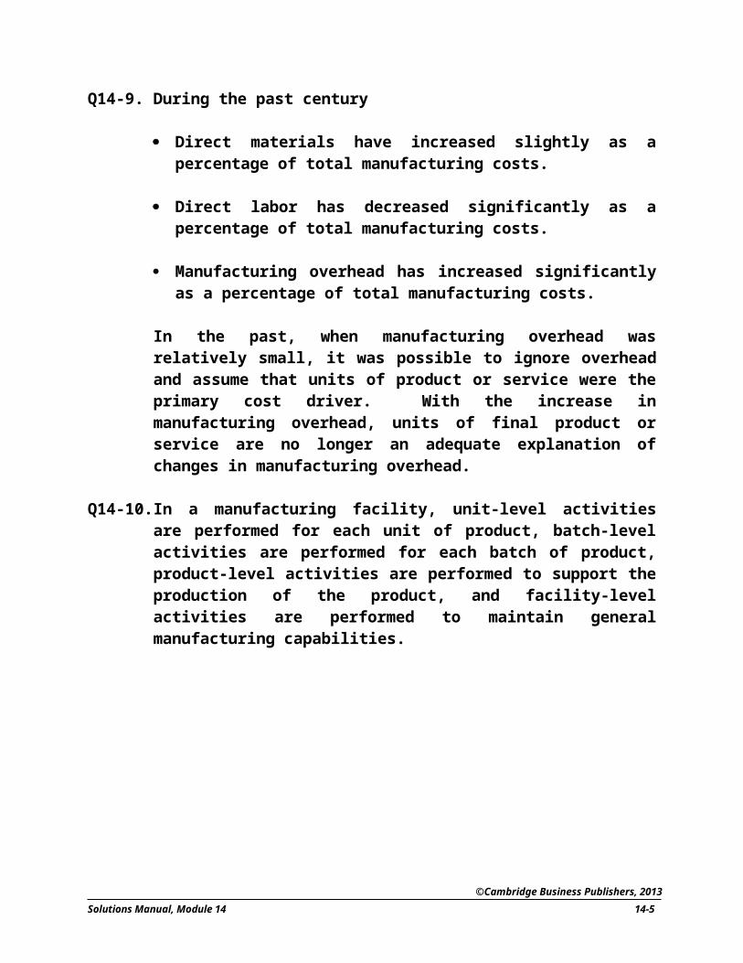
Q14-9. During the past century

Direct materials have increased slightly as a percentage of total manufacturing costs.

Direct labor has decreased significantly as a percentage of total manufacturing costs.

Manufacturing overhead has increased significantly as a percentage of total manufacturing costs.

In the past, when manufacturing overhead was relatively small, it was possible to ignore overhead and assume that units of product or service were the primary cost driver. With the increase in manufacturing overhead, units of final product or service are no longer an adequate explanation of changes in manufacturing overhead.

Q14-10. In a manufacturing facility, unit-level activities are performed for each unit of product, batch-level activities are performed for each batch of product, product-level activities are performed to support the production of the product, and facility-level activities are performed to maintain general manufacturing capabilities.



MINI-EXERCISES

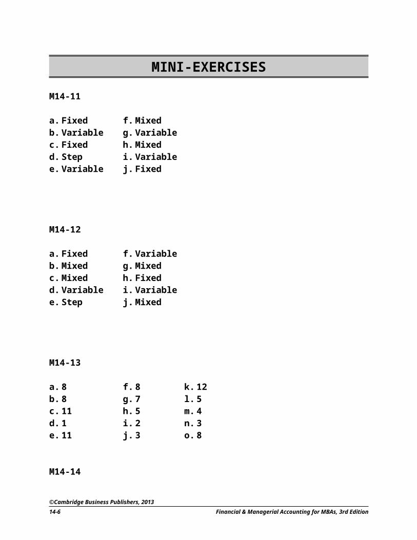
M14-11

a. Fixed f. Mixed b. Variable g. Variable c. Fixed h. Mixed d. Step i. Variable e. Variable j. Fixed

M14-12

a. Fixed f. Variable b. Mixed g. Mixedc. Mixed h. Fixedd. Variable i. Variablee. Step j. Mixed

M14-13

a. 8 f. 8 k. 12b. 8 g. 7 l. 5c. 11 h. 5 m. 4d. 1 i. 2 n. 3e. 11 j. 3 o. 8

M14-14

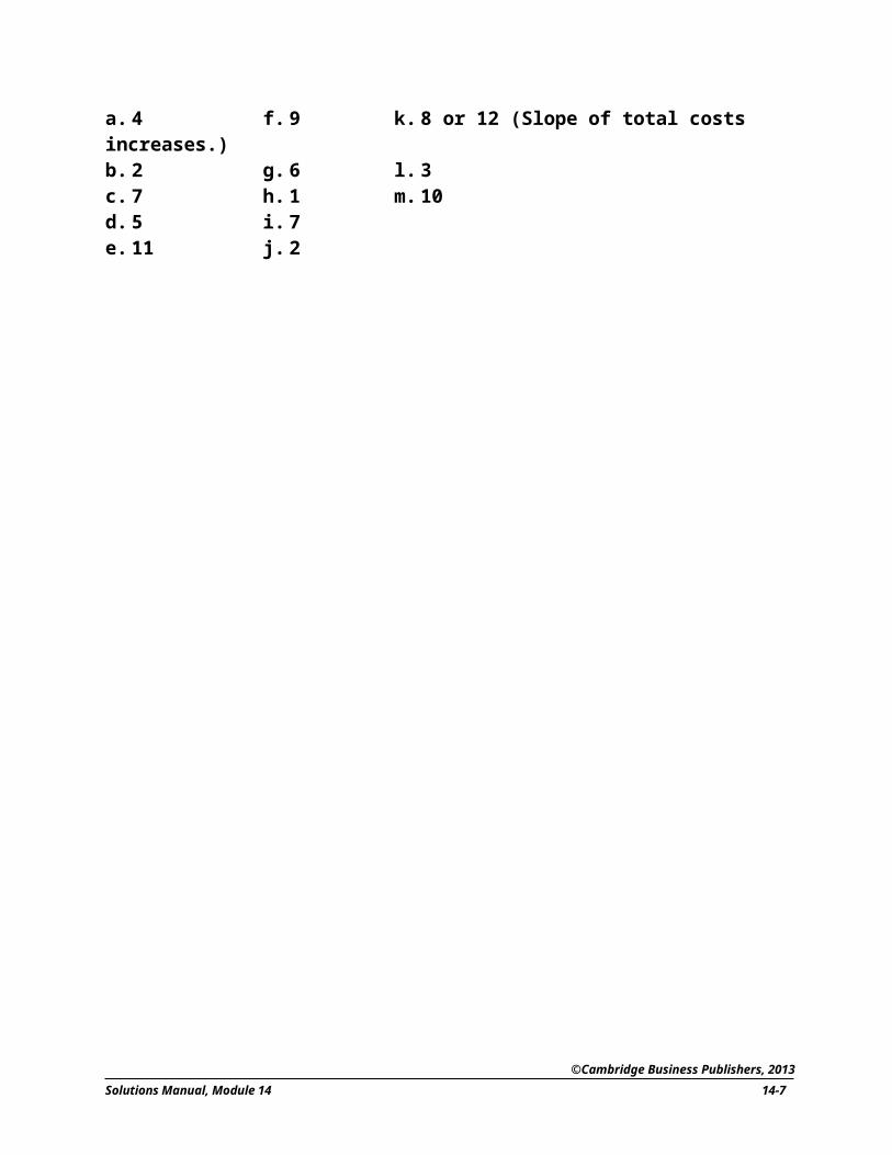
a. 4 f. 9 k. 8 or 12 (Slope of total costs increases.)b. 2 g. 6 l. 3c. 7 h. 1 m. 10d. 5 i. 7e. 11 j. 2



EXERCISES

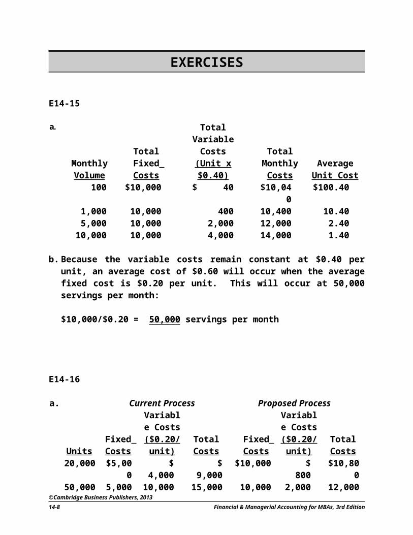
E14-15

a.Monthly Volume

Total Fixed Costs

Total Variable Costs(Unit x $0.40)

Total Monthly Costs

Average Unit Cost

100 $10,000 $ 40 $10,040 $100.401,000 10,000 400 10,400 10.405,000 10,000 2,000 12,000 2.40

10,000 10,000 4,000 14,000 1.40

b. Because the variable costs remain constant at $0.40 per unit, an average cost of $0.60 will occur when the average fixed cost is $0.20 per unit. This will occur at 50,000 servings per month:

$10,000/$0.20 = 50,000 servings per month

E14-16

a. Current Process Proposed Process

UnitsFixed Costs

Variable Costs($0.20/unit)

Total Costs

Fixed Costs

Variable Costs($0.20/unit)

TotalCosts

20,000 $5,000 $ 4,000 $ 9,000 $10,000 $ 800 $10,80050,000 5,000 10,000 15,000 10,000 2,000 12,000



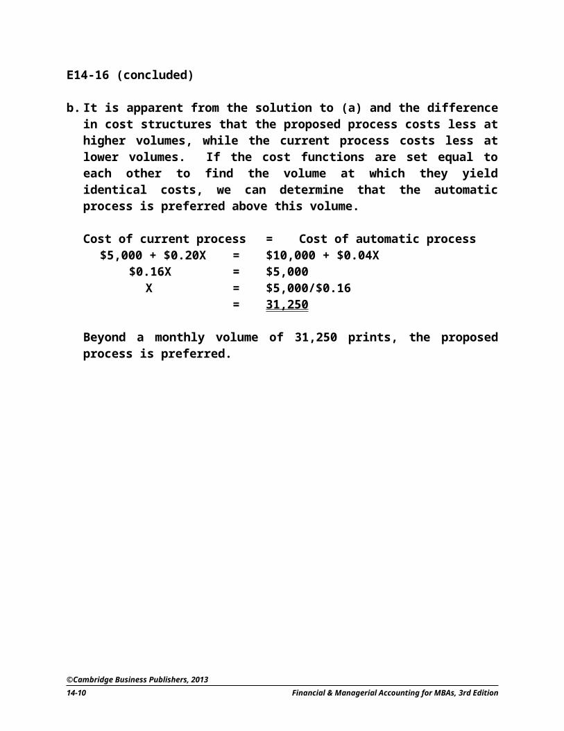
E14-16 (concluded)

b. It is apparent from the solution to (a) and the difference in cost structures that the proposed process costs less at higher volumes, while the current process costs less at lower volumes. If the cost functions are set equal to each other to find the volume at which they yield identical costs, we can determine that the automatic process is preferred above this volume.

Cost of current process = Cost of automatic process$5,000 + $0.20X = $10,000 + $0.04X

$0.16X = $5,000X = $5,000/$0.16

= 31,250

Beyond a monthly volume of 31,250 prints, the proposed process is preferred.



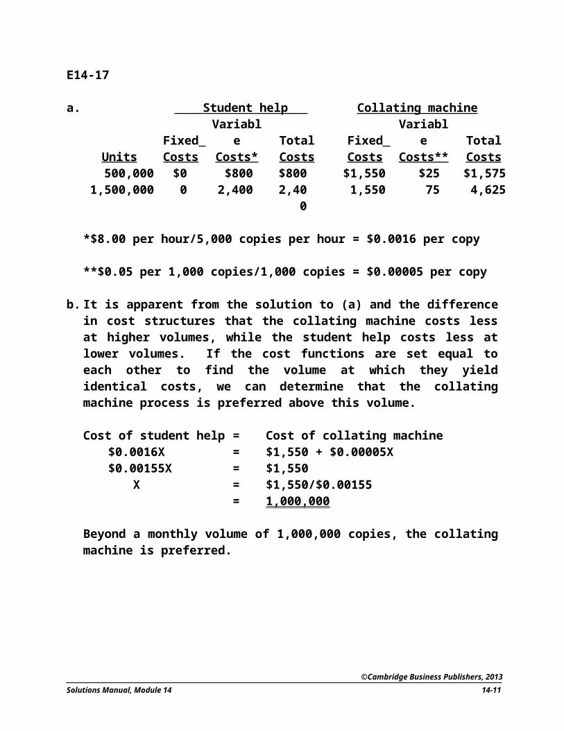
E14-17

a. Student help Collating machine

UnitsFixed Costs

Variable Costs*

Total Costs

Fixed Costs

Variable Costs**

TotalCosts

500,000 $0 $800 $800 $1,550 $25 $1,5751,500,000 0 2,400 2,400 1,550 75 4,625

*$8.00 per hour/5,000 copies per hour = $0.0016 per copy

**$0.05 per 1,000 copies/1,000 copies = $0.00005 per copy

b. It is apparent from the solution to (a) and the difference in cost structures that the collating machine costs less at higher volumes, while the student help costs less at lower volumes. If the cost functions are set equal to each other to find the volume at which they yield identical costs, we can determine that the collating machine process is preferred above this volume.

Cost of student help = Cost of collating machine$0.0016X = $1,550 + $0.00005X$0.00155X = $1,550

X = $1,550/$0.00155= 1,000,000

Beyond a monthly volume of 1,000,000 copies, the collating machine is preferred.



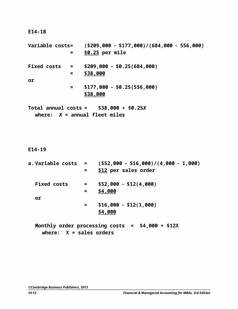
E14-18

Variable costs = ($209,000 $177,000)/(684,000 556,000)= $0.25 per mile

Fixed costs = $209,000 $0.25(684,000)= $38,000

or= $177,000 $0.25(556,000)

$38,000

Total annual costs = $38,000 + $0.25Xwhere: X = annual fleet miles

E14-19

a. Variable costs = ($52,000 $16,000)/(4,000 1,000)= $12 per sales order

Fixed costs = $52,000 $12(4,000)= $4,000

or= $16,000 $12(1,000)

$4,000

Monthly order processing costs = $4,000 + $12Xwhere: X = sales orders



E14-19 (concluded)

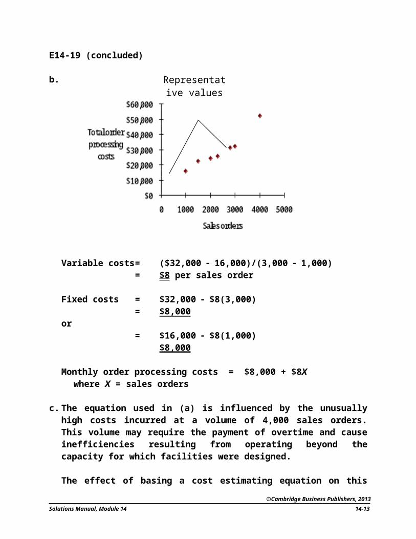
b.

Variable costs = ($32,000 16,000)/(3,000 1,000)= $8 per sales order

Fixed costs = $32,000 $8(3,000)= $8,000

or= $16,000 $8(1,000)

$8,000

Monthly order processing costs = $8,000 + $8Xwhere X = sales orders

c. The equation used in (a) is influenced by the unusually high costs incurred at a volume of 4,000 sales orders. This volume may require the payment of overtime and cause inefficiencies resulting from operating beyond the capacity for which facilities were designed.

The effect of basing a cost estimating equation on this observation is to overstate the variable costs and to understate the fixed costs.



Representative values

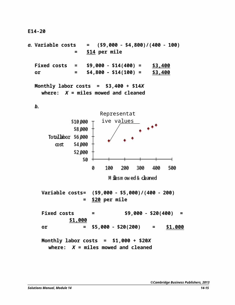
E14-20

a. Variable costs = ($9,000 $4,800)/(400 100)= $14 per mile

Fixed costs = $9,000 $14(400) = $3,400or = $4,800 $14(100) = $3,400

Monthly labor costs = $3,400 + $14Xwhere: X = miles mowed and cleaned

b.

Variable costs = ($9,000 $5,000)/(400 200)= $20 per mile

Fixed costs = $9,000 $20(400) = $1,000or = $5,000 $20(200) = $1.000

Monthly labor costs = $1,000 + $20Xwhere: X = miles mowed and cleaned



Representative values

E14-20 (concluded)

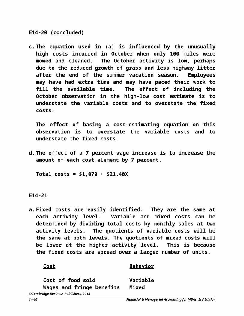
c. The equation used in (a) is influenced by the unusually high costs incurred in October when only 100 miles were mowed and cleaned. The October activity is low, perhaps due to the reduced growth of grass and less highway litter after the end of the summer vacation season. Employees may have had extra time and may have paced their work to fill the available time. The effect of including the October observation in the high-low cost estimate is to understate the variable costs and to overstate the fixed costs.

The effect of basing a cost-estimating equation on this observation is to overstate the variable costs and to understate the fixed costs.

d. The effect of a 7 percent wage increase is to increase the amount of each cost element by 7 percent.

Total costs = $1,070 + $21.40X

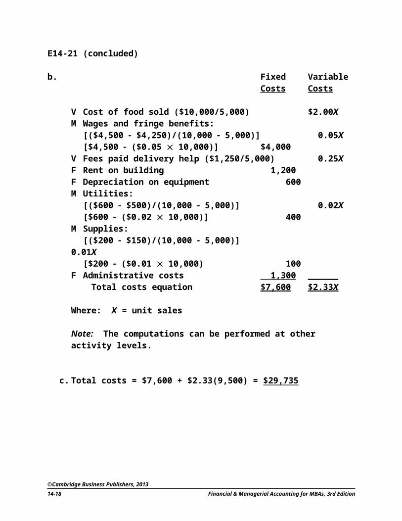
E14-21

a. Fixed costs are easily identified. They are the same at each activity level. Variable and mixed costs can be determined by dividing total costs by monthly sales at two activity levels. The quotients of variable costs will be the same at both levels. The quotients of mixed costs will be lower at the higher activity level. This is because the fixed costs are spread over a larger number of units.

Cost Behavior

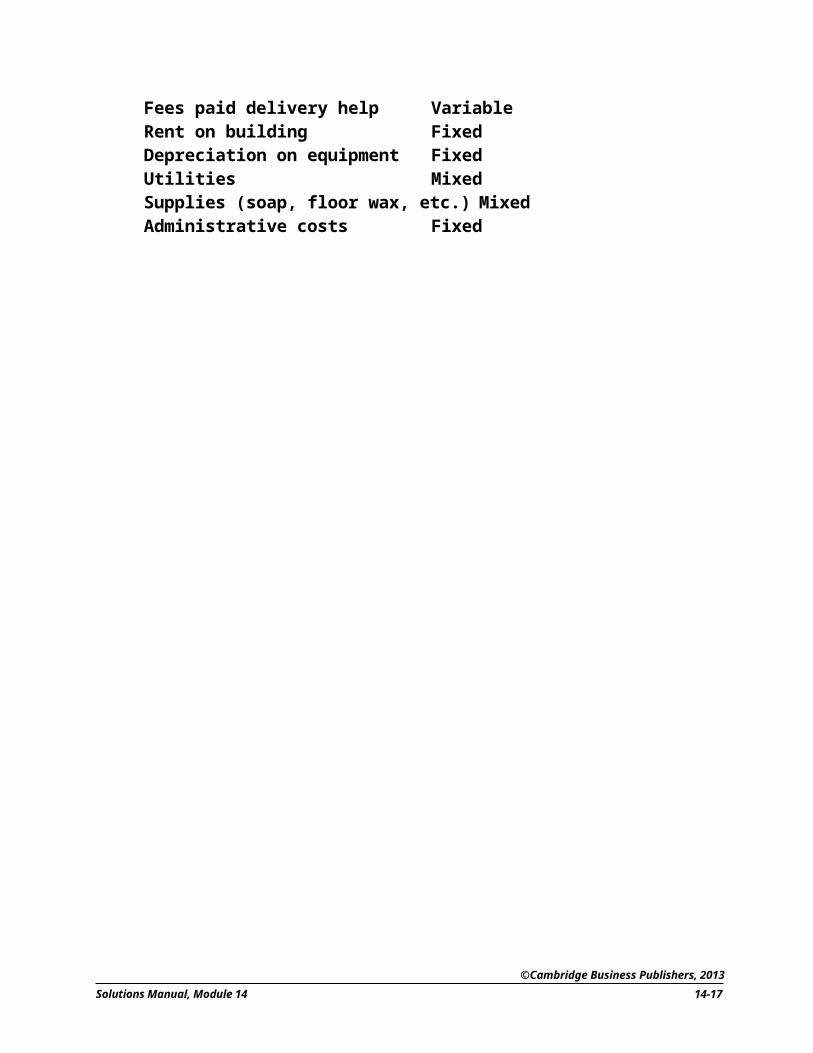
Cost of food sold VariableWages and fringe benefits MixedFees paid delivery help VariableRent on building FixedDepreciation on equipment FixedUtilities MixedSupplies (soap, floor wax, etc.) MixedAdministrative costs Fixed



E14-21 (concluded)

b. Fixed VariableCosts Costs

V Cost of food sold ($10,000/5,000) $2.00XM Wages and fringe benefits:

[($4,500 $4,250)/(10,000 5,000)] 0.05X[$4,500 ($0.05 10,000)] $4,000

V Fees paid delivery help ($1,250/5,000) 0.25XF Rent on building 1,200F Depreciation on equipment 600M Utilities:

[($600 $500)/(10,000 5,000)] 0.02X[$600 ($0.02 10,000)] 400

M Supplies:[($200 $150)/(10,000 5,000)] 0.01X[$200 ($0.01 10,000) 100

F Administrative costs 1,300 ______ Total costs equation $7,600 $2.33 X

Where: X = unit sales

Note: The computations can be performed at other activity levels.

c. Total costs = $7,600 + $2.33(9,500) = $29,735



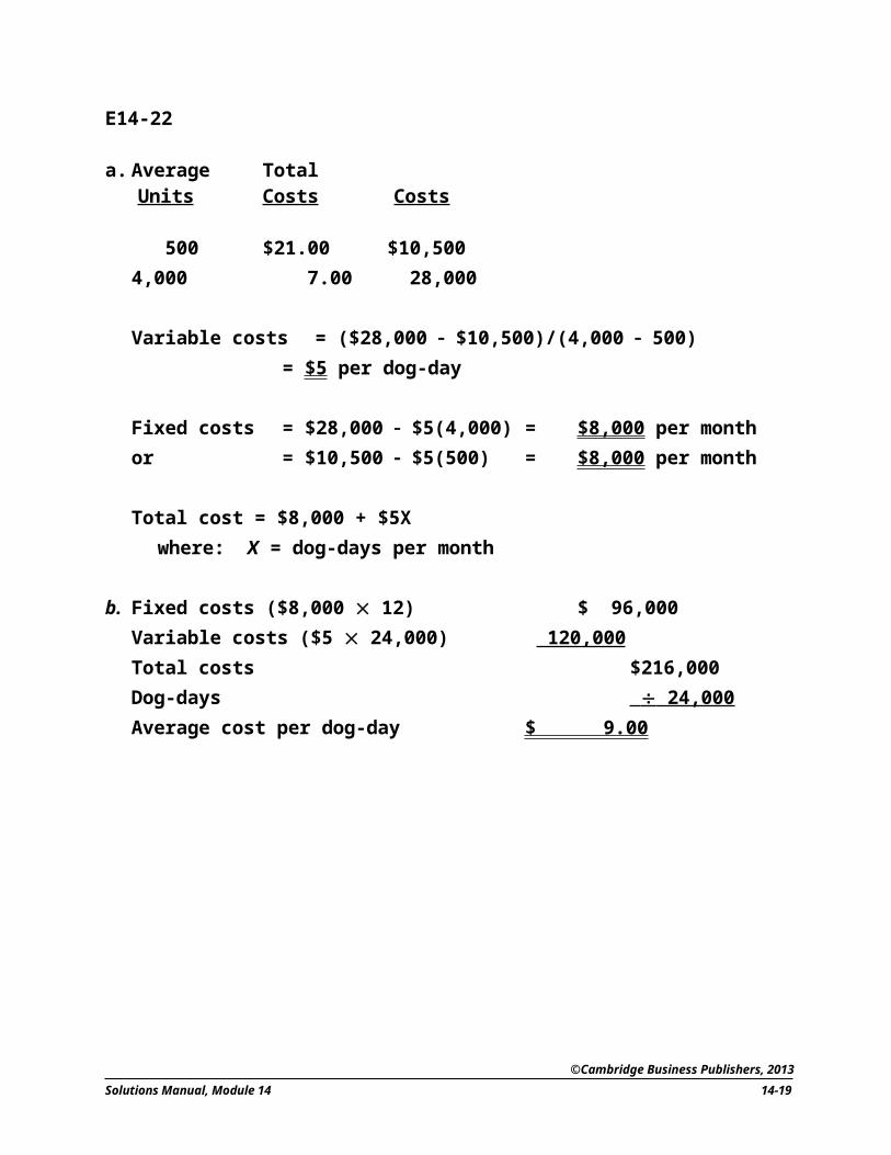
E14-22

a. Average TotalUnits Costs Costs

500 $21.00 $10,5004,000 7.00 28,000

Variable costs = ($28,000 $10,500)/(4,000 500)= $5 per dog-day

Fixed costs = $28,000 $5(4,000) = $8,000 per monthor = $10,500 $5(500) = $8,000 per month

Total cost = $8,000 + $5Xwhere: X = dog-days per month

b. Fixed costs ($8,000 12) $ 96,000Variable costs ($5 24,000) 120,000Total costs $216,000Dog-days 24,000 Average cost per dog-day $ 9.00



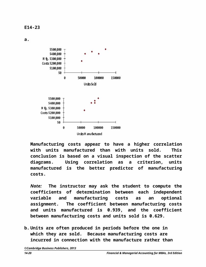
E14-23

a.

Manufacturing costs appear to have a higher correlation with units manufactured than with units sold. This conclusion is based on a visual inspection of the scatter diagrams. Using correlation as a criterion, units manufactured is the better predictor of manufacturing costs.

Note: The instructor may ask the student to compute the coefficients of determination between each independent variable and manufacturing costs as an optional assignment. The coefficient between manufacturing costs and units manufactured is 0.939, and the coefficient between manufacturing costs and units sold is 0.629.

b. Units are often produced in periods before the one in which they are sold. Because manufacturing costs are incurred in connection with the manufacture rather than the sale of products, it seems reasonable to expect that manufacturing costs will also have a higher correlation with units produced than they will with units sold.

c. Because selling costs are incurred in connection with selling rather than manufacturing activities, unit sales should be the better predictor of selling costs.



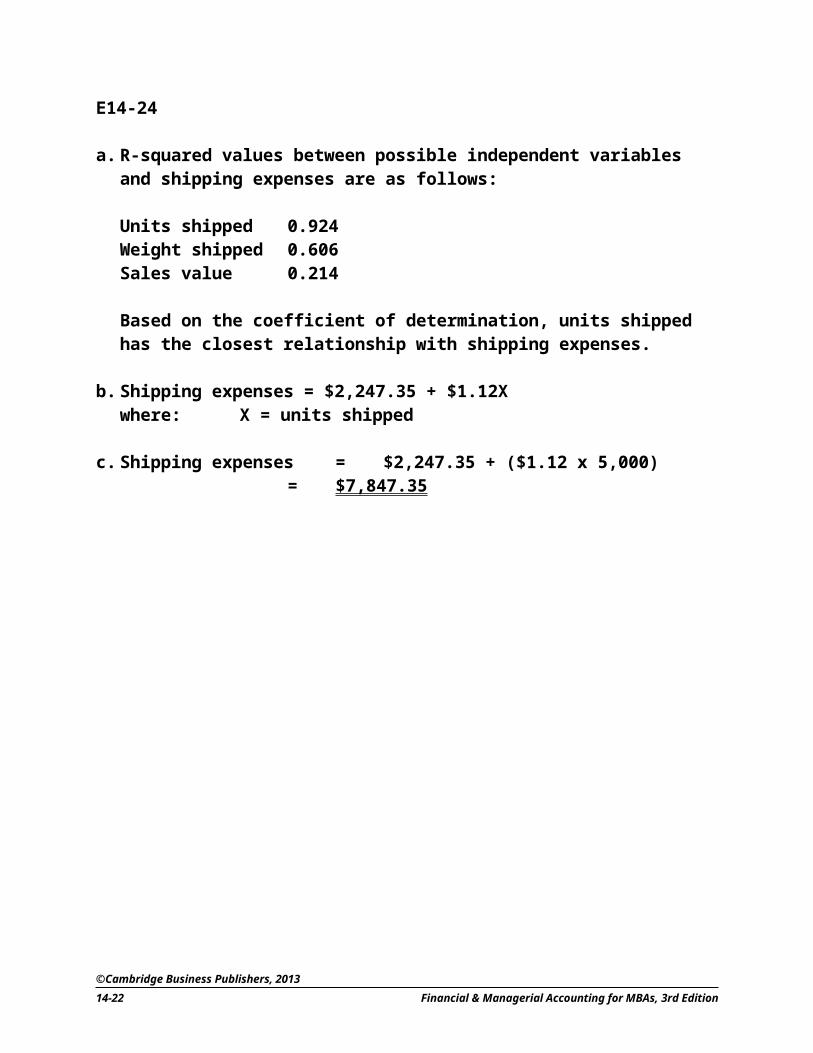
E14-24

a. R-squared values between possible independent variables and shipping expenses are as follows:

Units shipped 0.924Weight shipped 0.606Sales value 0.214

Based on the coefficient of determination, units shipped has the closest relationship with shipping expenses.

b. Shipping expenses = $2,247.35 + $1.12Xwhere: X = units shipped

c. Shipping expenses = $2,247.35 + ($1.12 x 5,000)= $7,847.35



PROBLEMS

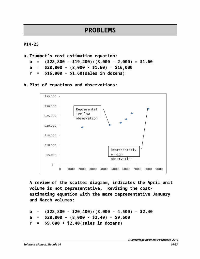
P14-25

a. Trumpet’s cost estimation equation:b = ($28,800 – $19,200)/(8,000 – 2,000) = $1.60a = $28,800 – (8,000 × $1.60) = $16,000Y = $16,000 + $1.60(sales in dozens)

b. Plot of equations and observations:

A review of the scatter diagram, indicates the April unit volume is not representative. Revising the cost-estimating equation with the more representative January and March volumes:

b = ($28,800 – $20,400)/(8,000 – 4,500) = $2.40a = $28,800 – (8,000 × $2.40) = $9,600Y = $9,600 + $2.40(sales in dozens)



Representative low observation

Representative high observation

P14-25 (concluded)

c. Which is a better predictor of future costs? Why?

The representative values identified with the aid of a scatter diagram provide a better cost-estimating equation and better predictor of future costs. This is because it omits the outlier observation at a volume of 2,000 units.

d. If you decided to develop a cost-estimating equation using the method of least squares, should you include all the observations? Why or why not?

No. The observation for 2,000 units should be omitted because it does not appear representative of normal operating conditions.

e. Reasons why the least-squares method is superior to the high-low and scatter diagram methods of cost estimation include. It is objective. It provides a measure of how well the cost-estimating equation

explains the variation in the dependent variable.



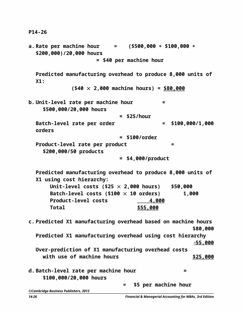
P14-26

a. Rate per machine hour =($500,000 + $100,000 + $200,000)/20,000 hours= $40 per machine hour

Predicted manufacturing overhead to produce 8,000 units of X1:($40 2,000 machine hours) = $80,000

b. Unit-level rate per machine hour = $500,000/20,000 hours= $25/hour

Batch-level rate per order = $100,000/1,000 orders = $100/order

Product-level rate per product = $200,000/50 products = $4,000/product

Predicted manufacturing overhead to produce 8,000 units of X1 using cost hierarchy:

Unit-level costs ($25 2,000 hours)$50,000 Batch-level costs ($100 10 orders) 1,000 Product-level costs 4,000 Total $55,000

c. Predicted X1 manufacturing overhead based on machine hours $80,000Predicted X1 manufacturing overhead using cost hierarchy 55,000 Over-prediction of X1 manufacturing overhead costs

with use of machine hours $25,000

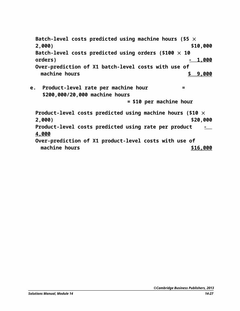
d. Batch-level rate per machine hour = $100,000/20,000 hours = $5 per machine hour

Batch-level costs predicted using machine hours ($5 2,000) $10,000Batch-level costs predicted using orders ($100 10 orders) 1,000 Over-prediction of X1 batch-level costs with use of

machine hours $ 9,000

e. Product-level rate per machine hour = $200,000/20,000 machine hours= $10 per machine hour

Product-level costs predicted using machine hours ($10 2,000) $20,000Product-level costs predicted using rate per product 4,000 Over-prediction of X1 product-level costs with use of

machine hours $16,000



P14-27

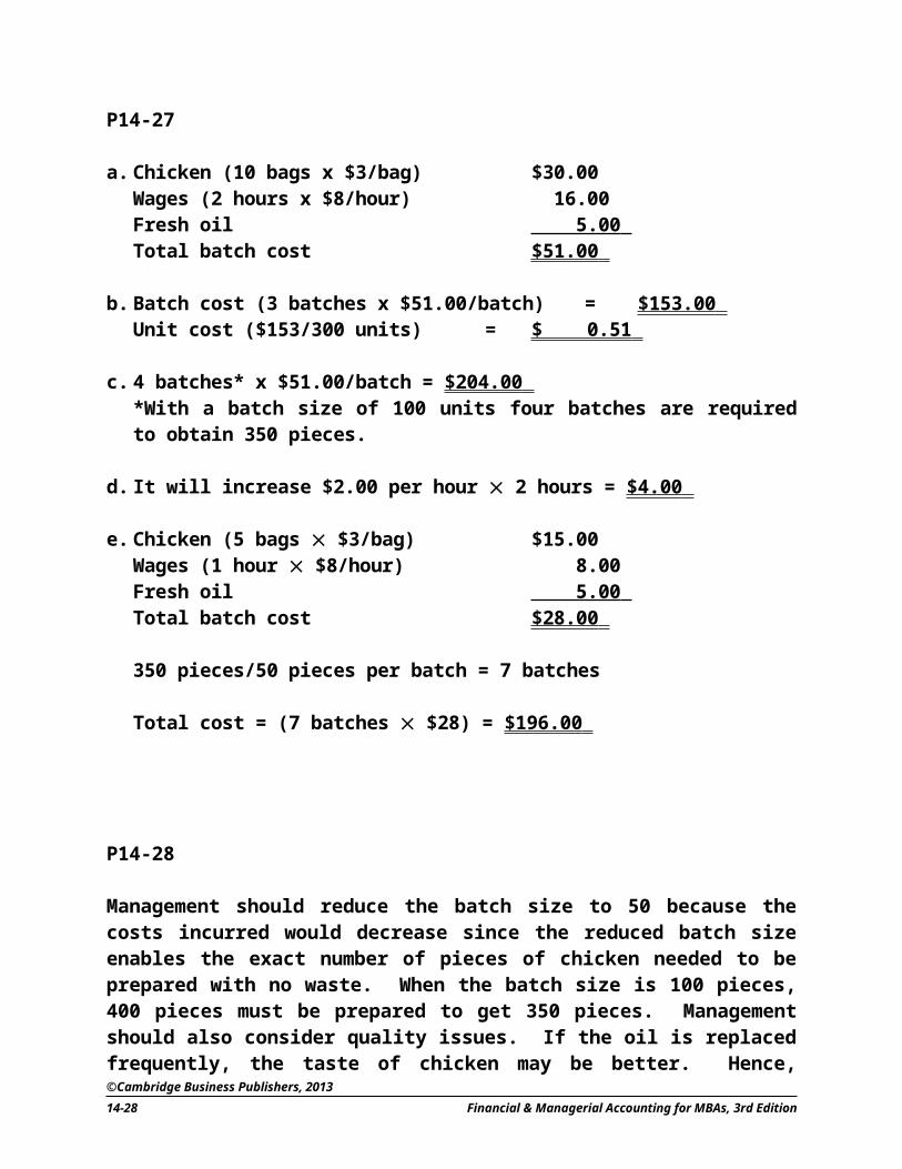
a. Chicken (10 bags x $3/bag) $30.00Wages (2 hours x $8/hour) 16.00Fresh oil 5.00 Total batch cost $51.00

b. Batch cost (3 batches x $51.00/batch) = $153.00 Unit cost ($153/300 units) = $ 0.51

c. 4 batches* x $51.00/batch = $204.00 *With a batch size of 100 units four batches are required to obtain 350 pieces.

d. It will increase $2.00 per hour 2 hours = $4.00

e. Chicken (5 bags $3/bag) $15.00Wages (1 hour $8/hour) 8.00Fresh oil 5.00 Total batch cost $28.00

350 pieces/50 pieces per batch = 7 batches

Total cost = (7 batches $28) = $196.00

P14-28

Management should reduce the batch size to 50 because the costs incurred would decrease since the reduced batch size enables the exact number of pieces of chicken needed to be prepared with no waste. When the batch size is 100 pieces, 400 pieces must be prepared to get 350 pieces. Management should also consider quality issues. If the oil is replaced frequently, the taste of chicken may be better. Hence, producing 50-piece batches may result in both lower cost and better quality. Management should also be sure to follow Health Department regulations.



MANAGEMENT APPLICATIONS

MA14-29

The negative “fixed costs” were obtained by fitting a cost estimating line through observed data. The negative “fixed costs” are better viewed as a constant term. The true cost function changes in some unknown way beyond the range of observations. Even though the constant term is negative, it may still be used to predict costs within the relevant range.

MA14-30

Mr. Morris’s reaction may be appropriate in this case. Apparently the assistant engaged in a random search for a high R-squared, testing relationships that had no logical relationship. If enough random relationships are tested, the laws of probability indicate that, sooner or later, a high R-squared will be found. Relationships determined in this way are merely hypotheses and they should be verified on a second set of independent data.

Ultimately, it may be determined that pounds of scrap has a high R-squared with manufacturing overhead, but it does not seem to be a feasible basis for predicting manufacturing overhead. In order to do this, it would be necessary to predict scrap. This would cause predictions of overhead to be two steps removed from their cause — production.



MA14-31

a. Repairs and maintenance take place during periods of low production, perhaps because they are deferred until time is available or because the existence of a breakdown, requiring repairs, halts production.

Think of miles driven and maintenance costs on an automobile. A car cannot be driven as much on the day it is in the garage being repaired.

b. Weekly or monthly data might provide a better match of the relationship between production and repair costs. Production personnel might be asked how frequently machines need repairs under normal operating conditions. If it is weekly, then weekly data might be used.

MA14-32

Mike is in a difficult situation. There is a strong temptation to keep quiet and hope there is no problem. Perhaps the excess oil consumption was a random event. There is also a temptation to want to avoid detecting a pollution problem. If there is pollution, it might not be detected when X-Town is demolished and paved over; and if pollution is detected then, Mike will be in another position. If questioned at that later date, he could claim ignorance.

On the other hand, if there is a pollution problem that continues for a couple more years, the cost of cleanup will be much higher than if the problem is corrected immediately. The increased awareness of the dangers of ground water pollution and the corresponding increase in regulations make it very unlikely that an oil tank leakage problem will go detected. Hence, correcting the problem today will likely be significantly less expensive than correcting it at some future date when more oil has leaked and the leaked oil has traveled further.

No information is provided about the ethical climate set by top management. Mike would feel much more comfortable informing top management of the situation and making an appropriate recommendation if he believed top management wanted to do the right thing. On the other hand, if top management treated the bearers of bad news as “whistle-blowers,” he has some difficult decisions to make.



MA14-32 (concluded)

If Phoenix Management Company has a code of ethics, Mike should consult it. If a code is not available for Phoenix, he might consult the code for another business or professional organization.

The appropriate sequence of actions is outlined under the heading “Resolution of Ethical Conflict.” In this case, Mike should start by discussing the problem with his immediate supervisor. He should explain the situation, outline the financial aspects of the alternative actions, and point out the advantage of developing a reputation as a “good corporate citizen, concerned about the environment.” Such a reputation will make the development of shopping malls in new communities easier.

MA14-33

a. The relevant major assumption that limits the accuracy of the current cost estimating equation is that the volume of activity is the only cost driver.

b. Incorporating the hierarchy of activity costs into the cost estimating equation will improve the accuracy of cost predictions. The current equation erroneously assumes that all varieties of ice cream cost the same to produce, that all packaging costs vary with gallons, and that all distribution activities vary with gallons. Recognizing the variability in each of these cost elements improves accuracy.

c. A general form of a more accurate cost-estimating equation is as follows:

Y = b1iX1i + b2iX2i + b3iX3i + b4iX4i + b5 iX5i

Labels, descriptions, and examples of elements are:

Y = total costs per monthb1i, b2i, b3, b4i, b5i = cost per unit of cost driverX1i = unit-level driver, where the subscript i refers to a specific driver,

such as pounds of raw materialsX2i = batch-level driver, where the subscript i refers to a specific driver,

such as batch inspectionX3i = product-level driver, where the subscript “i” refers to a specific

driver, such as maintaining a supplier for special ingredients, perhaps almonds



X4i = customer driver, where the subscript “i” refers to a specific driver, such as packaging or advertising

X5 = facility-level drivers, where the subscript “i” refers to a specific driver, such as property taxes



MA14-34

a. The following results are obtained using a spreadsheet program:

Regression Output: Constant -3967.575

Std Err of Y EST 517.696R Squared 0.978No. of Observations 12Degrees of Freedom 7X Coefficient(s) 56.775 64.266 52.987 101.016Std Err of Coef. 9.462 9.835 6.184 7.699

The resulting cost estimation equation and the cost per unit of each service is as follows:

Y = –$3,967.58 + $56.78(X1) + $64.27(X2) + $52.99(X3) + $101.02(X4)

This equation explains 97.8 percent of the variation in total monthly costs.

b. A comparison of the proposed rates and the estimated variable costs is presented below:

Procedure X1 X2 X3 X4Proposed rate $45.00 $90.00 $60.00 $105.00Est. cost 56 .78 64 .27 52 .99 101 .02 Profit (loss) $(11 .78) $25 .73 $ 7 .01 $ 3 .98

The desirability of the proposal depends on the mix of services used by the employees of the local business. If the mix contained a significant portion of X1, the proposal might not be desirable. Perhaps the best recommendation is to negotiate on the rate for procedure X1 to make sure that service is profitable. Central City might even offer to reduce the rate on procedure X2 to obtain an increase in the rate for X1.

c. According to the given information, the proposed rates are significantly below the current rates. Hence, accepting the proposal would require turning away regular customers who pay more for the identical services. This is not logical. Central City should reject the proposal.



MA14-35

a. The high observation is April 2011 and the low observation is December 2011.

Slope = ($97,800 – $37,650)/(315 – 165) = $60,150/150 = $401

Vertical axis intercept = $97,800 – ($401 × 315) = ($28,515)

or

Vertical axis intercept = $37,650 – ($401 × 165) = ($28,515)

Cost estimating equation: Y = ($28,515) + $401X

The negative $28,515 does not represent what costs would be at a production level of zero. Rather this is merely a value that assists in fitting an equation through the high and low observations. Because the high-low method utilizes two unusual observations (highest and lowest activity) it is possible that an equation developed with the high-low method does not represent the actual cost behavior pattern. The scatter graph, developed below, assists in evaluating the high and low observations and selecting representative high and low observations.

b. The scatter diagram is as follows:

It appears the April 2011 observation is not representative of normal operating conditions and should be excluded from an analysis of costs under normal operating conditions.



MA14-35 (continued)

c. The high observation is now August 2010 while the low observation remains December 2011

Slope = ($60,630 – $37,650)/(285 – 165) = $22,980/120 = $191.50

Vertical axis intercept = $60,630 – ($191.50 × 285) = $6,052.50

or

Vertical axis intercept = $37,650 – ($191.50 × 165) = $6,052.50

Cost estimating equation: Y = $6,052.50 + $191.50X

The results are strikingly different from those obtained in part “a.” The vertical axis intercept is much higher, and a positive number, while the slope is smaller. Basically, the unusual high observation in part “a” pulled the high end of the equation up from what it should be.

d. Presented is a partial printout from an Excel spreadsheet, excluding the April 2011 observation, with items of interest highlighted in bold:

SUMMARY OUTPUTRegression Statistics

Multiple R 0.826789R Square 0.68358Adjusted R Square 0.663804Standard Error 4049.279Observations 18

CoefficientsStandard

Error t Stat P-valueIntercept 14001.1 6268.23112 2.233661 0.040133X Variable 1 158.3602 26.93540398 5.879258 2.33E-05



MA14-35 (continued)

A consideration of the data not presented in bold, although important in applications of regression analysis, is beyond the scope of this text where we focus on how cost data can be analyzed using regression analysis.

The cost estimating equation is:

Cost estimating equation: Y = $14,001.10 + $158.36X

This equation has two advantages over that developed in part “c.”It uses all observations (except April 2011), rather than just two representative observations.It provides information on how well the cost-estimating equation explains the variation in the dependent variable. In this case, the cost-estimating equation explains 68.358 percent of the variation in total manufacturing costs.

Because of the least-squares criteria, the analyst must evaluate the data used in regression analysis and exclude unusual observations. Otherwise, a single large squared deviation will have a disproportionate influence in the cost-estimating equation.



MA14-35 (concluded)

e. The key to solving requirement “e” is to recognize that all previous analysis failed to determine the separate influence of dining room table and kitchen tables on manufacturing costs. The offer of $220 per table is above the computations of the variable cost per table in parts “c” ($191.50) and “d” ($158.36). Hence, management might be tempted to accept the offer.

Using multiple regression analysis with two independent variables, rather than one, illustrates this would be a mistake. Presented is a partial printout from an Excel spreadsheet with two independent variables, with items of interest highlighted in bold:

SUMMARY OUTPUT

Regression Statistics

Multiple R 0.998593

R Square 0.997187Adjusted R Square 0.996812

Standard Error 394.3038

Observations 18

ANOVA

df SS MS FSignificance

F

Regression 2 8267760214.13E+0

8 2658.86 7.389E-20

Residual 15 233213225 155476

Total 17 829108153

CoefficientsStandard

Error t Stat P-value Lower 95%Upper 95%

Intercept 7888.485 628.412302 12.5530 2.33E-09 6549.0557 9227.91

X Variable 1 295.996 4.26693951 69.3696 3.16E-20 286.90125 305.091

X Variable 2 120.5055 2.78141943 43.3252 3.56E-17 114.57701 126.434

Variable 1 represents the variable cost of a dining room table while variable 2 represents the variable cost of a kitchen table. Hence, the variable cost of a dining room table, $295.996, exceeds the offer of $220 per table. Management should reject the offer.

If students do not have access to a computer and spreadsheet software, the instructor can assign the problem and provide the results of the



regression.



MA14-36

If students do not have access to a computer and spreadsheet software, the instructor can still assign the problem after providing them with the following output:

First, for simple regression analysis:

Regression Output:Constant 26.82222Std Err of Y Est 2.994439R Squared 0.481696No. of Observations 10Degrees of Freedom 8

X Coefficient 1.111111Std Err of Coef. 0.407492

Second, for multiple regression analysis:

Regression Output:Constant 9.646175Std Err of Y Est 0.66333R Squared 0.980925No. of Observations 10Degrees of Freedom 6

X Coefficient 1.258166 2.464264 2.600728Std Err of Coef. 0.09271 0.175571 0.14941

1. An important part of determining what Kevin should do is to determine how long it takes to recondition a desktop computer.

Based on total unit and total hour information for the past 10 weeks, the average time to repair a piece of electronic equipment is 2.7875 hours (446 total hours/160 total units).

This suggests he can recondition approximately 14 desktop computers per week (40 hours per week/2.7875 hours) to obtain total weekly revenues of $560 (14 computers $40 each) and monthly revenues of $2,240 ($560 4 weeks). Subtracting the rental fee of $200 leaves him with $2,040 to cover other costs such as extra utilities and wages.



MA14-36 (continued)

If he worked for the store, he would receive $1,760 per month ($11 40 hours 4 weeks).

Based on this analysis, there is a monthly advantage of $280 to accepting the contract.

One problem with this analysis is that it assumes that all pieces of electronic equipment require the same amount of time to recondition. It also assumes that all 40 hours are devoted to direct labor activities. It is likely that there are facility-level activities such as equipment maintenance, training, and paperwork.

2. Based on simple regression analysis, 26.822 facility-level hours are required each week. This leaves 13.178 (40 26.822) hours to work on computers. Simple regression analysis indicates that the marginal time to repair a piece of electronic equipment is 1.111 hours. Using the available time, approximately 12 (13.178/1.111) computers can be reconditioned each week to obtain total weekly revenues of $480 (12 computers $40 each) and monthly revenues of $1,920 ($480 4 weeks). Subtracting the rental fee of $200 leaves him with $1,720 to cover other costs such as extra utilities and wages.

If Kevin worked for the store, he would receive $1,760 per month.

Based on this analysis there is a monthly advantage of $40 for working for Radio Stuff.

While the simple regression approach recognizes the existence of facility-level activities, it also assumes that all pieces of electronic equipment require the same amount of time to recondition.

An advantage of the regression approach is that we are provided with information on the goodness of fit. In this case the fit is not good. The coefficient of determination for the simple regression analysis is 0.481696, indicating that only 48.17% of the variation in total weekly hours is explained by the estimating equation. Hence, not much trust can be placed in these results.



MA14-36 (concluded)

3. Based on multiple regression analysis, 9.646 facility-level hours are required each week. This leaves 30.354 (40 9.646) hours to work on computers. Multiple regression analysis also indicates that the marginal time to repair a computer is 2.6 hours. Using the available time, approximately 12 (30.354 2.6) computers can be reconditioned each week to obtain total weekly revenues of $480 (12 computers $40 each) and monthly revenues of $1,920 ($480 4 weeks). Subtracting the rental fee of $200 leaves her with $1,720 to cover other costs such as extra utilities and wages.

If Kevin worked for the store he would receive $1,760 per month.

Based on this analysis there is a monthly advantage of $40 for working for Radio Stuff.

In this case, R-squared is 0.980925, implying that 98.09 percent of the variation in the dependent variable is explained by the cost-estimating equation.

Because of the small monthly advantage of working for Radio Stuff other considerations will likely be important in making a decision. Additional considerations include:

If Kevin can reduce the facility-level hours for setup and administrative activities and recondition 3 or 4 more computers, the economics would suggest accepting the contract.

Kevin may find that by reducing his travel time to and from work he is able to devote additional time to reconditioning computers. This might change the economics of accepting the contract.

There are quality-of-work issues. Working at home, Kevin can set his own hours. On the other hand, having a regular job provides some social interaction and clearly separates work from non-work activities.

Working at home requires a higher level of self-motivation than going to a more traditional job.

Fringe benefits are not mentioned in the case. If the store provides fringe benefits, such as health care and retirement benefits, the economics would clearly favor not accepting the contract.

Travel costs are not mentioned in the case. If they are high, this would favor working at home.

Note: To avoid complexities related to self-employment taxes they are



not considered in this assignment. Some students might mention self-employment taxes as an additional consideration.

