NAGARJUNA COLLEGE OF ENGINEERING AND TECHOLOGY COMPUTER SCIENCE AND ENGINEERING

Big Data

(16CSI732)

Module 2

NoSQL data management -1

By,

PRIYANKA K

Asst. Professor

CSE,NCET

NOSQL DATA MANAGEMENT -1

What is NoSQL?

NoSQL is a non-relational DBMS, that does not require a fixed schema, avoids joins, and

is easy to scale. The purpose of using a NoSQL database is for distributed data stores with

humongous data storage needs. NoSQL is used for Big data and real-time web apps. For

example, companies like Twitter, Facebook, Google collect terabytes of user data every single

day.

NoSQL database stands for "Not Only SQL" or "Not SQL." Though a better term would be

"NoREL", NoSQL caught on. Carl Strozz introduced the NoSQL concept in 1998.

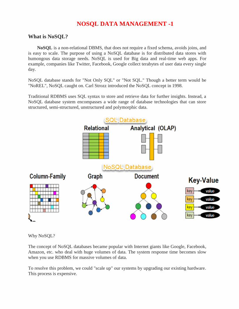
Traditional RDBMS uses SQL syntax to store and retrieve data for further insights. Instead, a

NoSQL database system encompasses a wide range of database technologies that can store

structured, semi-structured, unstructured and polymorphic data.

Why NoSQL?

The concept of NoSQL databases became popular with Internet giants like Google, Facebook,

Amazon, etc. who deal with huge volumes of data. The system response time becomes slow

when you use RDBMS for massive volumes of data.

To resolve this problem, we could "scale up" our systems by upgrading our existing hardware.

This process is expensive.

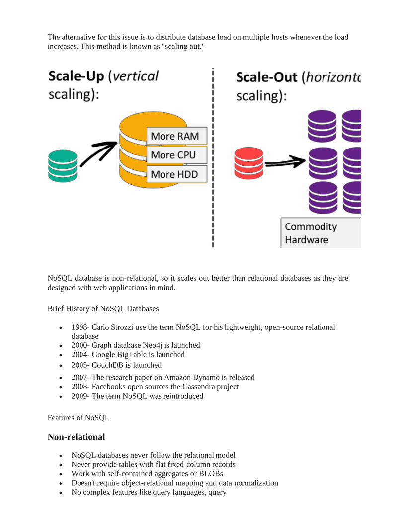
The alternative for this issue is to distribute database load on multiple hosts whenever the load

increases. This method is known as "scaling out."

NoSQL database is non-relational, so it scales out better than relational databases as they are

designed with web applications in mind.

Brief History of NoSQL Databases

• 1998- Carlo Strozzi use the term NoSQL for his lightweight, open-source relational database

• 2000- Graph database Neo4j is launched

• 2004- Google BigTable is launched

• 2005- CouchDB is launched

• 2007- The research paper on Amazon Dynamo is released

• 2008- Facebooks open sources the Cassandra project

• 2009- The term NoSQL was reintroduced

Features of NoSQL

Non-relational

• NoSQL databases never follow the relational model

• Never provide tables with flat fixed-column records

• Work with self-contained aggregates or BLOBs

• Doesn't require object-relational mapping and data normalization

• No complex features like query languages, query

• planners, referential integrity joins, ACID

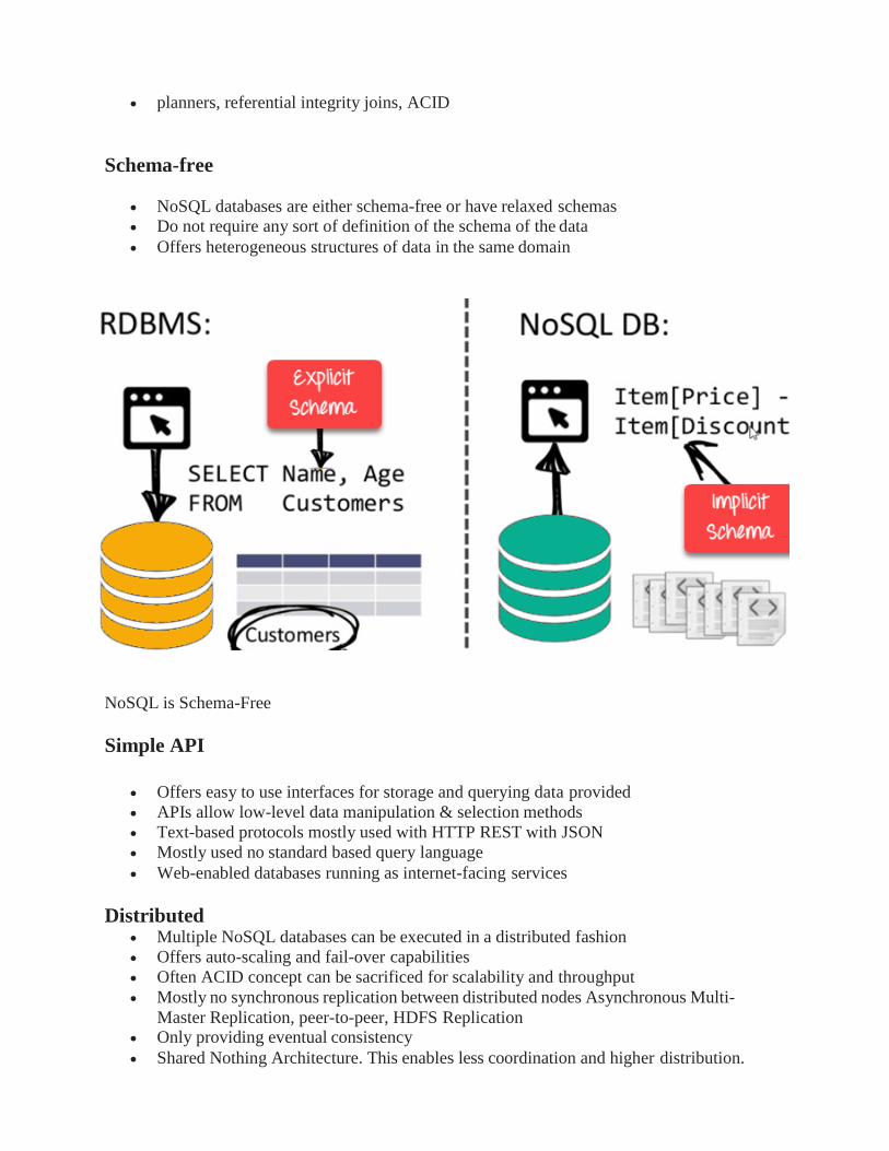
Schema-free

• NoSQL databases are either schema-free or have relaxed schemas

• Do not require any sort of definition of the schema of the data

• Offers heterogeneous structures of data in the same domain

NoSQL is Schema-Free

Simple API

• Offers easy to use interfaces for storage and querying data provided

• APIs allow low-level data manipulation & selection methods

• Text-based protocols mostly used with HTTP REST with JSON

• Mostly used no standard based query language

• Web-enabled databases running as internet-facing services

Distributed • Multiple NoSQL databases can be executed in a distributed fashion

• Offers auto-scaling and fail-over capabilities

• Often ACID concept can be sacrificed for scalability and throughput

• Mostly no synchronous replication between distributed nodes Asynchronous Multi-

Master Replication, peer-to-peer, HDFS Replication • Only providing eventual consistency

• Shared Nothing Architecture. This enables less coordination and higher distribution.

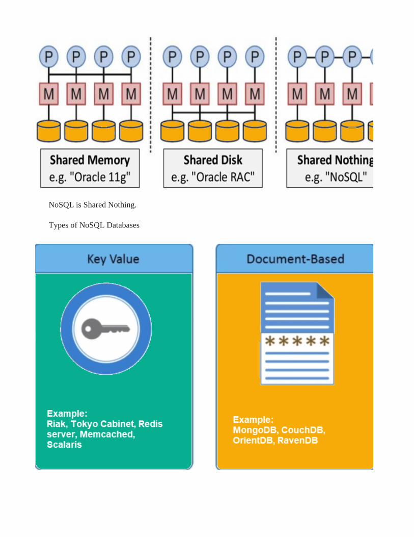
NoSQL is Shared Nothing.

Types of NoSQL Databases

There are mainly four categories of NoSQL databases. Each of these categories has its unique

attributes and limitations. No specific database is better to solve all problems. You should

select a database based on your product needs.

Let see all of them:

• Key-value Pair Based

• Column-oriented Graph

• Graphs based

• Document-oriented

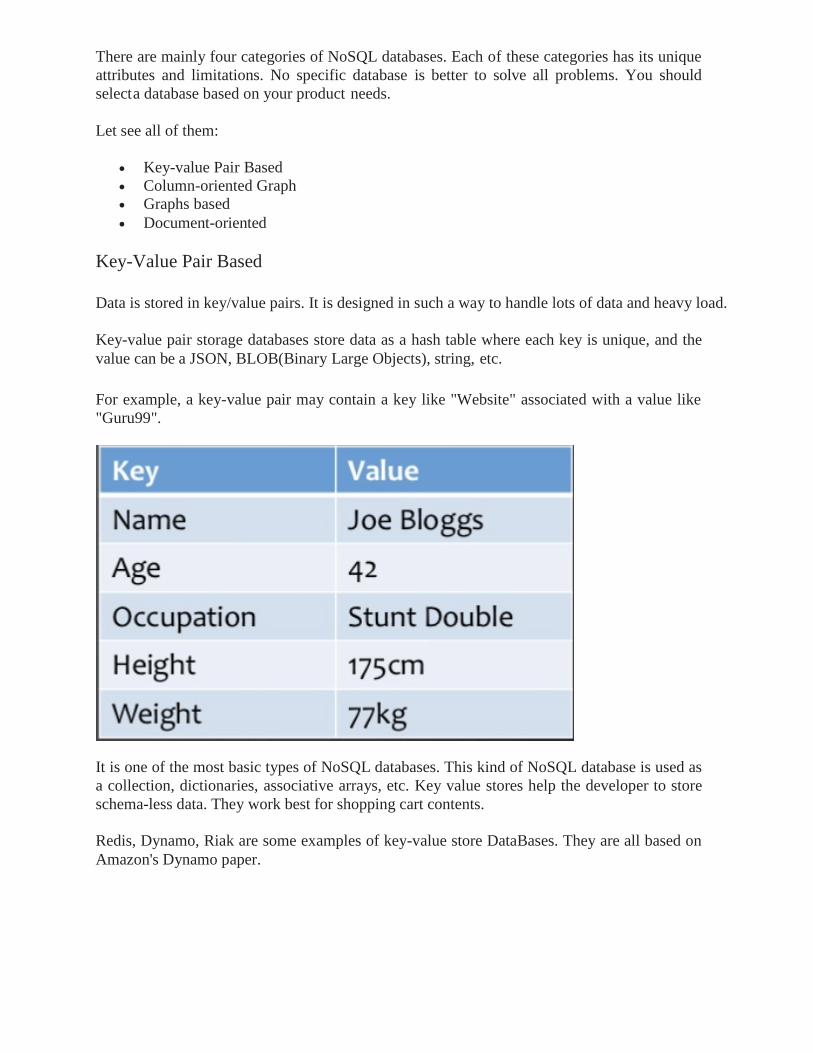
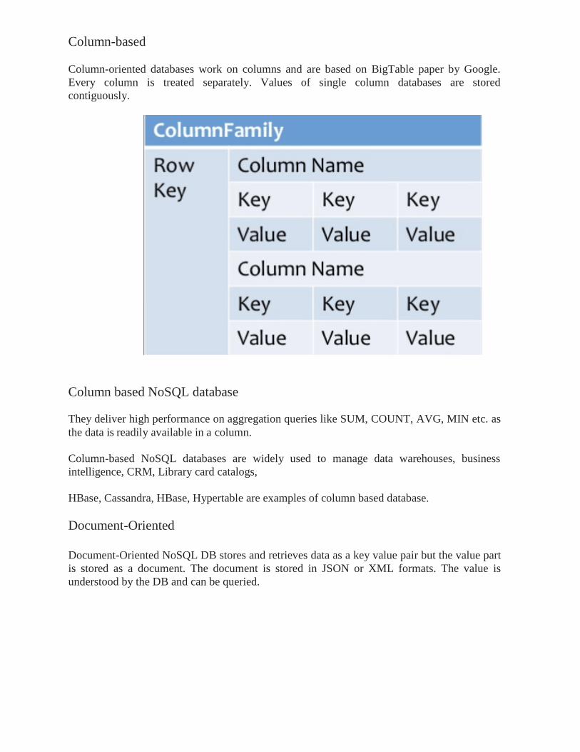
Key-Value Pair Based

Data is stored in key/value pairs. It is designed in such a way to handle lots of data and heavy load.

Key-value pair storage databases store data as a hash table where each key is unique, and the

value can be a JSON, BLOB(Binary Large Objects), string, etc.

For example, a key-value pair may contain a key like "Website" associated with a value like

"Guru99".

It is one of the most basic types of NoSQL databases. This kind of NoSQL database is used as

a collection, dictionaries, associative arrays, etc. Key value stores help the developer to store

schema-less data. They work best for shopping cart contents.

Redis, Dynamo, Riak are some examples of key-value store DataBases. They are all based on

Amazon's Dynamo paper.

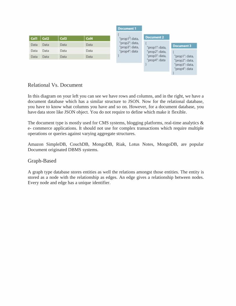
Column-based

Column-oriented databases work on columns and are based on BigTable paper by Google.

Every column is treated separately. Values of single column databases are stored

contiguously.

Column based NoSQL database

They deliver high performance on aggregation queries like SUM, COUNT, AVG, MIN etc. as

the data is readily available in a column.

Column-based NoSQL databases are widely used to manage data warehouses, business

intelligence, CRM, Library card catalogs,

HBase, Cassandra, HBase, Hypertable are examples of column based database.

Document-Oriented

Document-Oriented NoSQL DB stores and retrieves data as a key value pair but the value part

is stored as a document. The document is stored in JSON or XML formats. The value is

understood by the DB and can be queried.

Relational Vs. Document

In this diagram on your left you can see we have rows and columns, and in the right, we have a

document database which has a similar structure to JSON. Now for the relational database,

you have to know what columns you have and so on. However, for a document database, you

have data store like JSON object. You do not require to define which make it flexible.

The document type is mostly used for CMS systems, blogging platforms, real-time analytics &

e- commerce applications. It should not use for complex transactions which require multiple

operations or queries against varying aggregate structures.

Amazon SimpleDB, CouchDB, MongoDB, Riak, Lotus Notes, MongoDB, are popular

Document originated DBMS systems.

Graph-Based

A graph type database stores entities as well the relations amongst those entities. The entity is

stored as a node with the relationship as edges. An edge gives a relationship between nodes.

Every node and edge has a unique identifier.

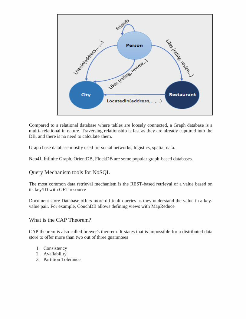
Compared to a relational database where tables are loosely connected, a Graph database is a

multi- relational in nature. Traversing relationship is fast as they are already captured into the

DB, and there is no need to calculate them.

Graph base database mostly used for social networks, logistics, spatial data.

Neo4J, Infinite Graph, OrientDB, FlockDB are some popular graph-based databases.

Query Mechanism tools for NoSQL

The most common data retrieval mechanism is the REST-based retrieval of a value based on

its key/ID with GET resource

Document store Database offers more difficult queries as they understand the value in a key-

value pair. For example, CouchDB allows defining views with MapReduce

What is the CAP Theorem?

CAP theorem is also called brewer's theorem. It states that is impossible for a distributed data

store to offer more than two out of three guarantees

1. Consistency

2. Availability

3. Partition Tolerance

Consistency:

The data should remain consistent even after the execution of an operation. This means once

data is written, any future read request should contain that data. For example, after updating

the order status, all the clients should be able to see the same data.

Availability:

The database should always be available and responsive. It should not have any downtime.

Partition Tolerance:

Partition Tolerance means that the system should continue to function even if the

communication among the servers is not stable. For example, the servers can be partitioned

into multiple groups which may not communicate with each other. Here, if part of the database

is unavailable, other parts are always unaffected.

Eventual Consistency

The term "eventual consistency" means to have copies of data on multiple machines to get

high availability and scalability. Thus, changes made to any data item on one machine has to

be propagated to other replicas.

Data replication may not be instantaneous as some copies will be updated immediately while

others in due course of time. These copies may be mutually, but in due course of time, they

become consistent. Hence, the name eventual consistency.

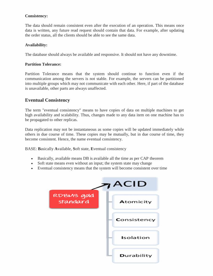
BASE: Basically Available, Soft state, Eventual consistency

• Basically, available means DB is available all the time as per CAP theorem

• Soft state means even without an input; the system state may change

• Eventual consistency means that the system will become consistent over time

Advantages of NoSQL

• Can be used as Primary or Analytic Data Source

• Big Data Capability

• No Single Point of Failure

• Easy Replication

• No Need for Separate Caching Layer

• It provides fast performance and horizontal scalability.

• Can handle structured, semi-structured, and unstructured data with equal effect

• Object-oriented programming which is easy to use and flexible

• NoSQL databases don't need a dedicated high-performance server

• Support Key Developer Languages and Platforms

• Simple to implement than using RDBMS

• It can serve as the primary data source for online applications.

• Handles big data which manages data velocity, variety, volume, and complexity

• Excels at distributed database and multi-data center operations

• Eliminates the need for a specific caching layer to store data

• Offers a flexible schema design which can easily be altered without downtime or

service disruption

Disadvantages of NoSQL

• No standardization rules

• Limited query capabilities

• RDBMS databases and tools are comparatively mature

• It does not offer any traditional database capabilities, like consistency when multiple transactions are performed simultaneously.

• When the volume of data increases it is difficult to maintain unique values as keys

become difficult

• Doesn't work as well with relational data

• The learning curve is stiff for new developers

• Open source options so not so popular for enterprises.

Aggregate data models

One of the first topics to spring to mind as we worked on Nosql Distilled was that NoSQL

databases use different data models than the relational model. Most sources I've looked at

mention at least four groups of data model: key-value, document, column-family, and graph.

Looking at this list, there's a big similarity between the first three - all have a fundamental unit

of storage which is a rich structure of closely related data: for key-value stores it's the value,

for document stores it's the document, and for column-family stores it's the column family. In

DDD terms, this group of data is an DDD_Aggregate.

The rise of NoSQL databases has been driven primarily by the desire to store data effectively

on large clusters - such as the setups used by Google and Amazon. Relational databases were

not designed with clusters in mind, which is why people have cast around for an alternative.

Storing

aggregates as fundamental units makes a lot of sense for running on a cluster. Aggregates

make natural units for distribution strategies such as sharding, since you have a large clump of

data that you expect to be accessed together.

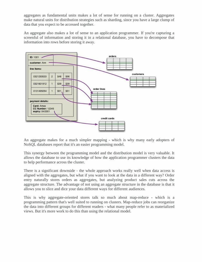
An aggregate also makes a lot of sense to an application programmer. If you're capturing a

screenful of information and storing it in a relational database, you have to decompose that

information into rows before storing it away.

An aggregate makes for a much simpler mapping - which is why many early adopters of

NoSQL databases report that it's an easier programming model.

This synergy between the programming model and the distribution model is very valuable. It

allows the database to use its knowledge of how the application programmer clusters the data

to help performance across the cluster.

There is a significant downside - the whole approach works really well when data access is

aligned with the aggregates, but what if you want to look at the data in a different way? Order

entry naturally stores orders as aggregates, but analyzing product sales cuts across the

aggregate structure. The advantage of not using an aggregate structure in the database is that it

allows you to slice and dice your data different ways for different audiences.

This is why aggregate-oriented stores talk so much about map-reduce - which is a

programming pattern that's well suited to running on clusters. Map-reduce jobs can reorganize

the data into different groups for different readers - what many people refer to as materialized

views. But it's more work to do this than using the relational model.

This is part of the argument for PolyglotPersistence - use aggregate-oriented databases when

you are manipulating clear aggregates (especially if you are running on a cluster) and use

relational databases (or a graph database) when you want to manipulate that data in different

ways.

Aggregate Data Models

• An aggregate is a collection of data that we interact with as a unit. Aggregates form the

boundaries for ACID operations with the database.

• Key-value, document, and column-family databases can all be seen as forms of

aggregate- oriented database.

• Aggregates make it easier for the database to manage data storage over clusters.

• Aggregate-oriented databases work best when most data interaction is done with the same aggregate; aggregate-ignorant databases are better when interactions use data

organized in many different formations.

Distributed Database System

A distributed database is basically a database that is not limited to one system, it is spread

over different sites, i.e., on multiple computers or over a network of computers. A

distributed database system is located on various sited that don’t share physical components.

This may be required when a particular database needs to be accessed by various users

globally. It needs to be managed such that for the users it looks like one single database.

Types:

1. Homogeneous Database:

In a homogeneous database, all different sites store database identically. The operating

system, database management system and the data structures used – all are same at all

sites. Hence, they’re easy to manage.

2. Heterogeneous Database:

In a heterogeneous distributed database, different sites can use different schema and

software that can lead to problems in query processing and transactions. Also, a particular

site might be completely unaware of the other sites. Different computers may use a

different operating system, different database application. They may even use different data

models for the database. Hence, translations are required for different sites to

communicate.

Distributed Data Storage

There are 2 ways in which data can be stored on different sites. These are:

1. Replication In this approach, the entire relation is stored redundantly at 2 or more sites. If the entire

database is available at all sites, it is a fully redundant database. Hence, in replication, systems

maintain copies of data. This is advantageous as it increases the availability of data

at different sites. Also, now query requests can be processed in parallel. However, it has

certain disadvantages as well. Data needs to be constantly updated. Any change made at one

site needs to be recorded at every site that relation is stored or else it may lead to

inconsistency. This is a lot of overhead. Also, concurrency control becomes way more complex

as concurrent access now needs to be checked over a number of sites.

2. Fragmentation In this approach, the relations are fragmented (i.e., they’re divided into smaller parts) and each

of the fragments is stored in different sites where they’re required. It must be made sure that

the fragments are such that they can be used to reconstruct the original relation (i.e., there isn’t

any loss of data).

Fragmentation is advantageous as it doesn’t create copies of data, consistency is not a problem. Fragmentation of relations can be done in two ways:

• Horizontal fragmentation – Splitting by rows – The relation is fragmented into groups of

tuples so that each tuple is assigned to at least one fragment.

• Vertical fragmentation – Splitting by columns – The schema of the relation is divided into

smaller schemas. Each fragment must contain a common candidate key so as to ensure

lossless join.

In certain cases, an approach that is hybrid of fragmentation and replication is used.

Distribution Models

There are two styles of distributing data:

• Sharding distributes different data across multiple servers, so each server acts as the

single source for a subset of data.

• Replication copies data across multiple servers, so each bit of data can be found in

multiple places.

A system may use either or both techniques.

Replication comes in two forms:

• -slave replication makes one node the authoritative copy that handles writes while slaves

synchronize with the master and may handle reads.

• Peer-to-peer replication allows writes to any node; the nodes coordinate to synchronize

Master their copies of the data.

Master-slave replication reduces the chance of update conflicts but peer-to-peer replication

avoids loading all writes onto a single point of failure.

Consistency

• Write-write conflicts occur when two clients try to write the same data at the same time.

Read-write conflicts occur when one client reads inconsistent data in the middle of

another client's write.

• Pessimistic approaches lock data records to prevent conflicts. Optimistic approaches

detect conflicts and fix them.

• Distributed systems see read-write conflicts due to some nodes having received updates

while other nodes have not. Eventual consistency means that at some point the system

will become consistent once all the writes have propagated to all the nodes.

• Clients usually want read-your-writes consistency, which means a client can write and

then immediately read the new value. This can be difficult if the read and the write

happen on different nodes.

• To get good consistency, you need to involve many nodes in data operations, but this

increases latency. So you often have to trade off consistency versus latency.

• The CAP theorem states that if you get a network partition, you have to trade off availability of data versus consistency.

• Durability can also be traded off against latency, particularly if you want to survive

failures with replicated data.

• You do not need to contact all replicants to preserve strong consistency with replication; you just need a large enough quorum.

Views: A View is a virtual relation that acts as an actual relation. It is not a part of logical relational

model of the database system. Tuples of the view are not stored in the database system and

tuples of the view are generated every time the view is accessed. Query expression of the view

is stored in the databases system.

Views can be used everywhere were we can use the actual relation. Views can be used to

create custom virtual relations according to the needs of a specific user. We can create as many

views as we want in a databases system.

Materialized Views: When the results of a view expression are stored in a database system, they are called

materialized views. SQL does not provides any standard way of defining materialized view,

however some database management system provides custom extensions to use materialized

views. The process of keeping the materialized views updated is know as view maintenance.

Database system uses one of the three ways to keep the materialized view updated:

• Update the materialized view as soon as the relation on which it is defined is updated.

• Update the materialized view every time the view is accessed.

• Update the materialized view periodically.

Materialized view is useful when the view is accessed frequently, as it saves the computation

time, as the result are stored in the database beforehand. Materialized view can also be helpful

in case where the relation on which view is defined is very large and the resulting relation of

the view is very small. Materialized view has storage cost and updating overheads associated

with it.

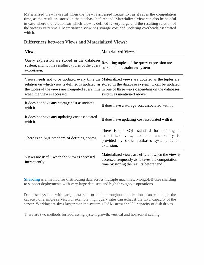
Differences between Views and Materialized Views:

Views Materialized Views

Query expression are stored in the databases

system, and not the resulting tuples of the query

expression.

Resulting tuples of the query expression are

stored in the databases system.

Views needs not to be updated every time the

relation on which view is defined is updated, as

the tuples of the views are computed every time

when the view is accessed.

Materialized views are updated as the tuples are

stored in the database system. It can be updated

in one of three ways depending on the databases

system as mentioned above.

It does not have any storage cost associated

with it.

It does have a storage cost associated with it.

It does not have any updating cost associated

with it.

It does have updating cost associated with it.

There is an SQL standard of defining a view.

There is no SQL standard for defining a

materialized view, and the functionality is

provided by some databases systems as an

extension.

Views are useful when the view is accessed

infrequently.

Materialized views are efficient when the view is

accessed frequently as it saves the computation

time by storing the results beforehand.

Sharding is a method for distributing data across multiple machines. MongoDB uses sharding to support deployments with very large data sets and high throughput operations.

Database systems with large data sets or high throughput applications can challenge the

capacity of a single server. For example, high query rates can exhaust the CPU capacity of the

server. Working set sizes larger than the system’s RAM stress the I/O capacity of disk drives.

There are two methods for addressing system growth: vertical and horizontal scaling.

Vertical Scaling involves increasing the capacity of a single server, such as using a more

powerful CPU, adding more RAM, or increasing the amount of storage space. Limitations in

available technology may restrict a single machine from being sufficiently powerful for a

given workload. Additionally, Cloud-based providers have hard ceilings based on available

hardware configurations. As a result, there is a practical maximum for vertical scaling.

Horizontal Scaling involves dividing the system dataset and load over multiple servers,

adding additional servers to increase capacity as required. While the overall speed or capacity

of a single machine may not be high, each machine handles a subset of the overall workload,

potentially providing better efficiency than a single high-speed high-capacity server.

Expanding the capacity of the deployment only requires adding additional servers as needed,

which can be a lower overall cost than high-end hardware for a single machine. The tradeoff is

increased complexity in infrastructure and maintenance for the deployment.

Version Stamps

• Version stamps help you detect concurrency conflicts. When you read data, then update

it, you can check the version stamp to ensure nobody updated the data between your

read and write.

• Version stamps can be implemented using counters, GUIDs, content hashes, timestamps, or a combination of these.

• With distributed systems, a vector of version stamps allows you to detect when different

nodes have conflicting updates.

Map-Reduce

• Map-reduce is a pattern to allow computations to be parallelized over a cluster.

• The map task reads data from an aggregate and boils it down to relevant key-value pairs.

Maps only read a single record at a time and can thus be parallelized and run on the

node that stores the record.

• Reduce tasks take many values for a single key output from map tasks and summarize

them into a single output. Each reducer operates on the result of a single key, so it can be

parallelized by key.

• Reducers that have the same form for input and output can be combined into pipelines.

This improves parallelism and reduces the amount of data to be transferred.

• Map-reduce operations can be composed into pipelines where the output of one reduce

is the input to another operation's map.

• If the result of a map-reduce computation is widely used, it can be stored as a

materialized view.

• Materialized views can be updated through incremental map-reduce operations that only

compute changes to the view instead of recomputing everything from scratch.

Partitioning

A partitioner works like a condition in processing an input dataset. The partition phase takes

place after the Map phase and before the Reduce phase.

The number of partitioners is equal to the number of reducers. That means a partitioner will

divide the data according to the number of reducers. Therefore, the data passed from a single

partitioner is processed by a single Reducer.

Partitioner

A partitioner partitions the key-value pairs of intermediate Map-outputs. It partitions the data

using a user-defined condition, which works like a hash function. The total number of

partitions is same as the number of Reducer tasks for the job. Let us take an example to

understand how the partitioner works.

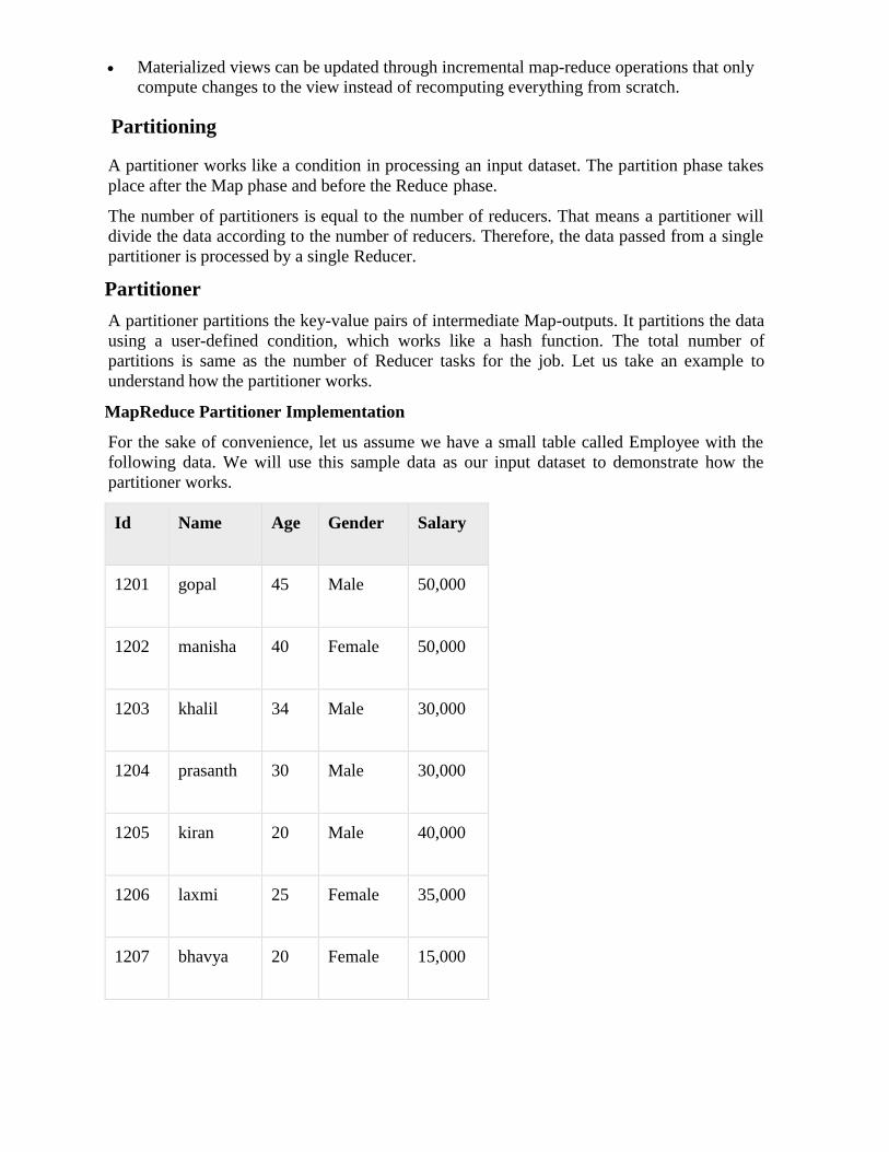
MapReduce Partitioner Implementation

For the sake of convenience, let us assume we have a small table called Employee with the

following data. We will use this sample data as our input dataset to demonstrate how the

partitioner works.

Id Name Age Gender Salary

1201 gopal 45 Male 50,000

1202 manisha 40 Female 50,000

1203 khalil 34 Male 30,000

1204 prasanth 30 Male 30,000

1205 kiran 20 Male 40,000

1206 laxmi 25 Female 35,000

1207 bhavya 20 Female 15,000

1208 reshma 19 Female 15,000

1209 kranthi 22 Male 22,000

1210 Satish 24 Male 25,000

1211 Krishna 25 Male 25,000

1212 Arshad 28 Male 20,000

1213 lavanya 18 Female 8,000

We have to write an application to process the input dataset to find the highest salaried

employee by gender in different age groups (for example, below 20, between 21 to 30, above

30).

Input Data

The above data is saved as input.txt in the “/home/hadoop/hadoopPartitioner” directory and

given as input.

1201 gopal 45 Male 50000

1202 manisha 40 Female 51000

1203 khaleel 34 Male 30000

1204 prasanth 30 Male 31000

1205 kiran 20 Male 40000

1206 laxmi 25 Female 35000

1207 bhavya 20 Female 15000

1208 reshma 19 Female 14000

1209 kranthi 22 Male 22000

1210 Satish 24 Male 25000

1211 Krishna 25 Male 26000

1212 Arshad 28 Male 20000

1213 lavanya 18 Female 8000

Based on the given input, following is the algorithmic explanation of the program.

Map Tasks

The map task accepts the key-value pairs as input while we have the text data in a text file.

The input for this map task is as follows −

Input − The key would be a pattern such as “any special key + filename + line number”

(example: key = @input1) and the value would be the data in that line (example: value = 1201

\t gopal \t 45

\t Male \t 50000).

Method − The operation of this map task is as follows −

• Read the value (record data), which comes as input value from the argument list in a string.

• Using the split function, separate the gender and store in a string

variable. String[] str = value.toString().split("\t", -3);

String gender=str[3];

• Send the gender information and the record data value as output key-value pair from

the map task to the partition task.

context.write(new Text(gender), new Text(value));

• Repeat all the above steps for all the records in the text file.

Output − You will get the gender data and the record data value as key-value pairs.

if(age<=20)

{

return 0;

}

else if(age>20 && age<=30)

{

return 1 % numReduceTasks;

}

else

{

return 2 % numReduceTasks;

}

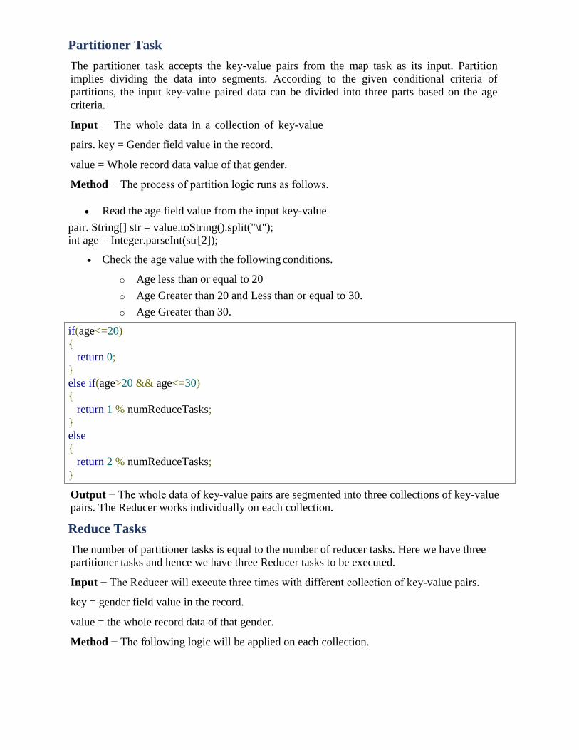
Partitioner Task

The partitioner task accepts the key-value pairs from the map task as its input. Partition

implies dividing the data into segments. According to the given conditional criteria of

partitions, the input key-value paired data can be divided into three parts based on the age

criteria.

Input − The whole data in a collection of key-value

pairs. key = Gender field value in the record.

value = Whole record data value of that gender.

Method − The process of partition logic runs as follows.

• Read the age field value from the input key-value

pair. String[] str = value.toString().split("\t"); int age = Integer.parseInt(str[2]);

• Check the age value with the following conditions.

o Age less than or equal to 20

o Age Greater than 20 and Less than or equal to 30.

o Age Greater than 30.

Output − The whole data of key-value pairs are segmented into three collections of key-value pairs. The Reducer works individually on each collection.

Reduce Tasks

The number of partitioner tasks is equal to the number of reducer tasks. Here we have three

partitioner tasks and hence we have three Reducer tasks to be executed.

Input − The Reducer will execute three times with different collection of key-value pairs.

key = gender field value in the record.

value = the whole record data of that gender.

Method − The following logic will be applied on each collection.

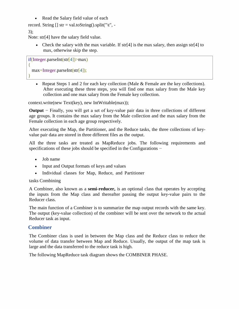
if(Integer.parseInt(str[4])>max)

{

max=Integer.parseInt(str[4]);

}

• Read the Salary field value of each

record. String [] str = val.toString().split("\t", -

3);

Note: str[4] have the salary field value.

• Check the salary with the max variable. If str[4] is the max salary, then assign str[4] to

max, otherwise skip the step.

• Repeat Steps 1 and 2 for each key collection (Male & Female are the key collections).

After executing these three steps, you will find one max salary from the Male key

collection and one max salary from the Female key collection.

context.write(new Text(key), new IntWritable(max));

Output − Finally, you will get a set of key-value pair data in three collections of different

age groups. It contains the max salary from the Male collection and the max salary from the

Female collection in each age group respectively.

After executing the Map, the Partitioner, and the Reduce tasks, the three collections of key-

value pair data are stored in three different files as the output.

All the three tasks are treated as MapReduce jobs. The following requirements and

specifications of these jobs should be specified in the Configurations −

• Job name

• Input and Output formats of keys and values

• Individual classes for Map, Reduce, and Partitioner

tasks Combining

A Combiner, also known as a semi-reducer, is an optional class that operates by accepting

the inputs from the Map class and thereafter passing the output key-value pairs to the

Reducer class.

The main function of a Combiner is to summarize the map output records with the same key.

The output (key-value collection) of the combiner will be sent over the network to the actual

Reducer task as input.

Combiner

The Combiner class is used in between the Map class and the Reduce class to reduce the

volume of data transfer between Map and Reduce. Usually, the output of the map task is

large and the data transferred to the reduce task is high.

The following MapReduce task diagram shows the COMBINER PHASE.

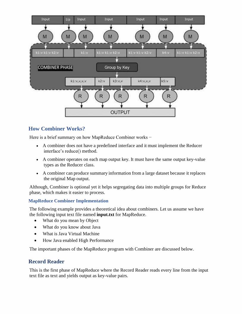
How Combiner Works?

Here is a brief summary on how MapReduce Combiner works −

• A combiner does not have a predefined interface and it must implement the Reducer

interface’s reduce() method.

• A combiner operates on each map output key. It must have the same output key-value

types as the Reducer class.

• A combiner can produce summary information from a large dataset because it replaces

the original Map output.

Although, Combiner is optional yet it helps segregating data into multiple groups for Reduce

phase, which makes it easier to process.

MapReduce Combiner Implementation

The following example provides a theoretical idea about combiners. Let us assume we have

the following input text file named input.txt for MapReduce.

• What do you mean by Object

• What do you know about Java

• What is Java Virtual Machine

• How Java enabled High Performance

The important phases of the MapReduce program with Combiner are discussed below.

Record Reader

This is the first phase of MapReduce where the Record Reader reads every line from the input

text file as text and yields output as key-value pairs.

public static class TokenizerMapper extends Mapper<Object, Text, Text, IntWritable>

{

private final static IntWritable one = new IntWritable(1);

private Text word = new Text();

public void map(Object key, Text value, Context context) throws IOException,

InterruptedException {

StringTokenizer itr = new StringTokenizer(value.toString());

while (itr.hasMoreTokens())

{

word.set(itr.nextToken());

context.write(word, one); }

}

}

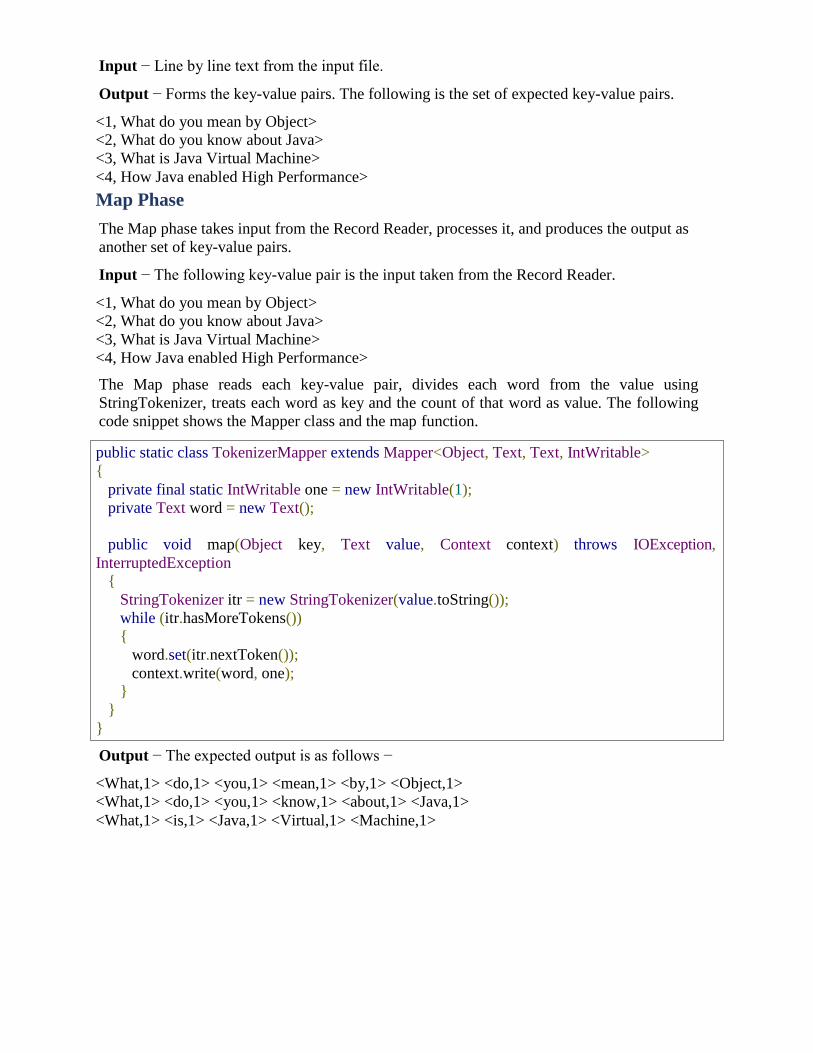
Input − Line by line text from the input file.

Output − Forms the key-value pairs. The following is the set of expected key-value pairs.

<1, What do you mean by Object>

<2, What do you know about Java>

<3, What is Java Virtual Machine>

<4, How Java enabled High Performance>

Map Phase

The Map phase takes input from the Record Reader, processes it, and produces the output as

another set of key-value pairs.

Input − The following key-value pair is the input taken from the Record Reader.

<1, What do you mean by Object>

<2, What do you know about Java>

<3, What is Java Virtual Machine>

<4, How Java enabled High Performance>

The Map phase reads each key-value pair, divides each word from the value using

StringTokenizer, treats each word as key and the count of that word as value. The following

code snippet shows the Mapper class and the map function.

Output − The expected output is as follows −

<What,1> <do,1> <you,1> <mean,1> <by,1> <Object,1>

<What,1> <do,1> <you,1> <know,1> <about,1> <Java,1>

<What,1> <is,1> <Java,1> <Virtual,1> <Machine,1>

public static class IntSumReducer extends Reducer<Text,IntWritable,Text,IntWritable>

{

private IntWritable result = new IntWritable();

public void reduce(Text key, Iterable<IntWritable> values,Context context) throws

IOException, InterruptedException {

int sum = 0;

for (IntWritable val : values)

{

<How,1> <Java,1> <enabled,1> <High,1> <Performance,1>

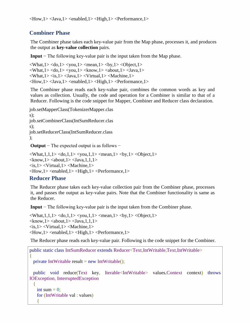
Combiner Phase

The Combiner phase takes each key-value pair from the Map phase, processes it, and produces

the output as key-value collection pairs.

Input − The following key-value pair is the input taken from the Map phase.

<What,1> <do,1> <you,1> <mean,1> <by,1> <Object,1>

<What,1> <do,1> <you,1> <know,1> <about,1> <Java,1>

<What,1> <is,1> <Java,1> <Virtual,1> <Machine,1>

<How,1> <Java,1> <enabled,1> <High,1> <Performance,1>

The Combiner phase reads each key-value pair, combines the common words as key and

values as collection. Usually, the code and operation for a Combiner is similar to that of a

Reducer. Following is the code snippet for Mapper, Combiner and Reducer class declaration.

job.setMapperClass(TokenizerMapper.clas

s);

job.setCombinerClass(IntSumReducer.clas

s);

job.setReducerClass(IntSumReducer.class

);

Output − The expected output is as follows −

<What,1,1,1> <do,1,1> <you,1,1> <mean,1> <by,1> <Object,1>

<know,1> <about,1> <Java,1,1,1>

<is,1> <Virtual,1> <Machine,1>

<How,1> <enabled,1> <High,1> <Performance,1>

Reducer Phase

The Reducer phase takes each key-value collection pair from the Combiner phase, processes

it, and passes the output as key-value pairs. Note that the Combiner functionality is same as

the Reducer.

Input − The following key-value pair is the input taken from the Combiner phase.

<What,1,1,1> <do,1,1> <you,1,1> <mean,1> <by,1> <Object,1>

<know,1> <about,1> <Java,1,1,1>

<is,1> <Virtual,1> <Machine,1>

<How,1> <enabled,1> <High,1> <Performance,1>

The Reducer phase reads each key-value pair. Following is the code snippet for the Combiner.

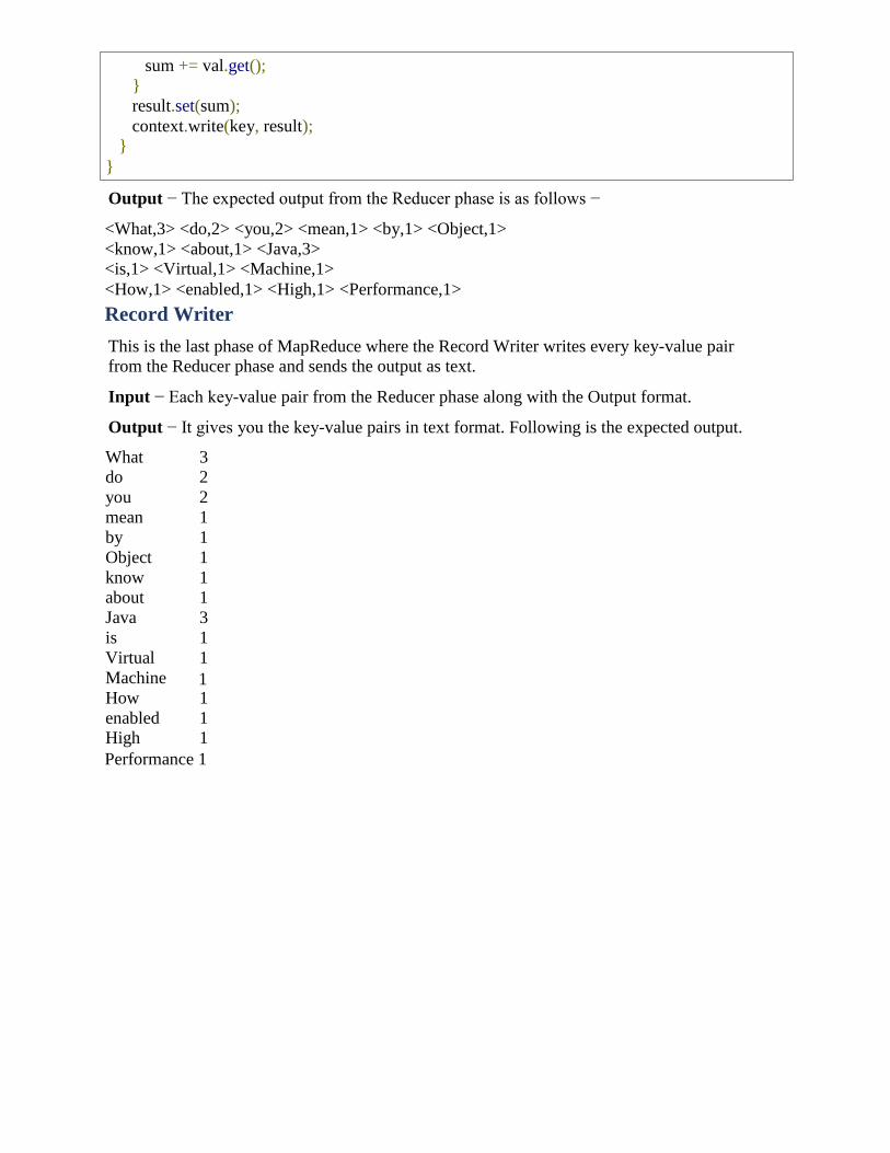
Output − The expected output from the Reducer phase is as follows −

<What,3> <do,2> <you,2> <mean,1> <by,1> <Object,1>

<know,1> <about,1> <Java,3>

<is,1> <Virtual,1> <Machine,1>

<How,1> <enabled,1> <High,1> <Performance,1>

Record Writer

This is the last phase of MapReduce where the Record Writer writes every key-value pair

from the Reducer phase and sends the output as text.

Input − Each key-value pair from the Reducer phase along with the Output format.

Output − It gives you the key-value pairs in text format. Following is the expected output.

What 3 do 2

you 2

mean 1

by 1

Object 1

know 1

about 1

Java 3

is 1

Virtual 1

Machine 1

How 1

enabled 1

High 1

Performance 1

sum += val.get();

}

result.set(sum);

context.write(key, result); }

}