module 3 exploring spreadsheets - pbworksteachit2009.pbworks.com/f/exploring+spreadsheets.pdf ·...

Module 3 Exploring Spreadsheets I

Learning Objectives

Pass1 Student is able to: Merit

1 Enter labels and numbers into a P spreadsheet

2 Enter and copy simple formulae P

3 Create a graph P

4 Modify data M

5 Use a spreadsheet to answer a M modelled scenario ('what if)

Exploring Spreadsheets 29

P-

3.1 What is a Learning Ob~ective: 1

Cells -

Put an X in each of these cells:

you made?

Columns and rows \

Drag along a row. r This is a column.1 Drag down a column.

- ~ ~~ ~~p

~~~, , ~ ~~

-. Exploring Spreadsheets 31

Learning Objectives: 1, 2 1 3.2 Autosum " -

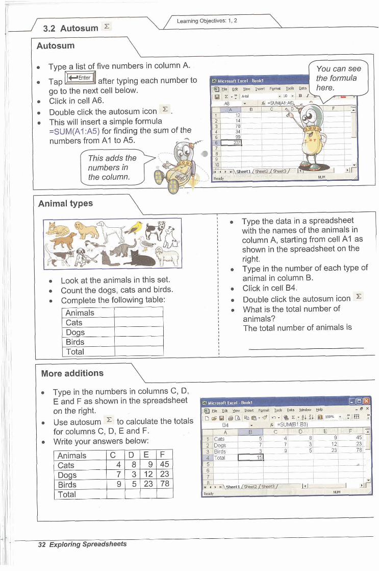
Type a list of five numbers in column A.

after typing each number to go to the next cell below. Click in cell A6.

numbers from A1 to A5.

: Type the data in a spreadsheet with the names of the animals in column A, starting from cell A1 as shown in the spreadsheet on the right. Type in the number of each type of

Look at the animals in this set. animal in column B.

Count the dogs, cats and birds. ! Click in cell B4. Complete the following table: \ Double click the autosum icon

Animals : . What is the total number of animals? The total number of animals is

Birds Total

More additions

Type in the numbers in columns C, D, E and F as shown in the spreadsheet on the right. Use autosum -I- to calculate the totals for columns C, D, E and F. Write your answers below:

32 Exploring Spreadsheets

3.3 Autofit Learning Objectives. 1, 2

Score Paulo Di Cario Joe Cole

Frederic Kanoute Trevor Sinclair Total

Football scores

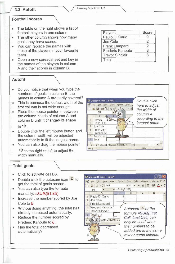
The table on the right shows a list of football players in one column. The other column shows how many goals they have scored. You can replace the names with those of the players in your favourite team. Open a new spreadsheet and key in the names of the players in column A and their scores in column B.

Autofit

Do you notice that when you type the numbers of goals in column B, the names in column A are partly covered? This is because the default width of the first column is not wide enough. Place the mouse pointer in between the column heads of column A and column B until it changes its shape

to Ct* . Double click the left mouse button and the column width will be adjusted automatically to fit the longest name. You can also drag the mouse pointer

Ct* to the right or left to adjust the width manually.

Total goals

Click to activate cell B6. Double click the autosum icon '" to get the total of goals scored. You can also type the formula manually: =SUM(Bl:B5) Increase the number scored by Joe Cole to 5. Without doing anything, the total has already increased automatically. formula =SUM(First Reduce the number scored by Cell: Last Cell) can Frederic Kanoute to 6. only be used when Has the total decreased the numbers to be automatically? added are in the same

row or same column.

! Microsoft Excel - Book4 Elk

I t


Learning Objective: 2 / 3.4 Typing formulae 7 / An adding machine \

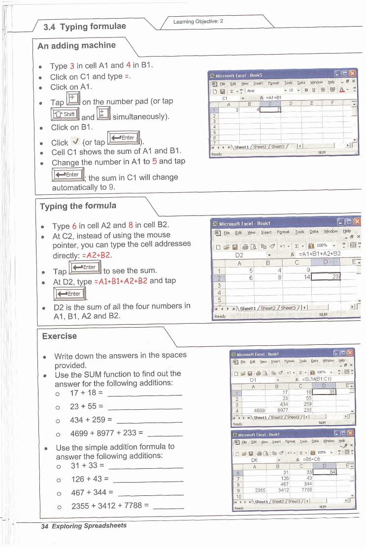
Type 3 in cell A1 and 4 in B1. Click on C1 and type =. Click on A l .

on the number pad (or tap

and simultaneously). Click on B1.

Click 4 (or tap ). Cell C1 shows the sum of A1 and B1.

e number in A1 to 5 and tap

the sum in C1 will change automatically to 9.

\

I Typing the formula \ Type 6 in cell A2 and 8 in cell B2. At C2, instead of using the mouse pointer, you can type the cell addresses

to see the sum. At D2, type =Al+Bl+A2+B2 and tap

D2 is the sum of all the four numbers in

\

Exercise

Write down the answers in the spaces provided. Use the SUM function to find out the answer for the following additions: o 17+18=

o 23 + 55 =

o 434 + 259 =

o 4699+8977+233=

Use the simple addition formula to answer the following additions: o 31 + 33 =

o 126+43=

o 467 + 344=

o 2355+3412+7788=


3.5 More for Learning Objective: 2

I / A subtraction machin\

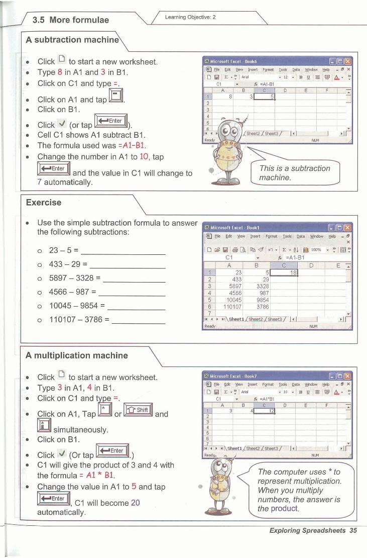
Click to start a new worksheet. Type 8 in A1 and 3 in B l . Click on C1 and tvoe =. , . Click on A1 and tap . Click on B1.

Click 'd. (or tap Cell C1 shows'~1 subtract B1. The formula used was =Al-B1. Change the number in A1 to 10, tap

and the value in C1 will change to - 7 automatically.

k a subtractionJ machine.

I

Exercise

Use the simple subtraction formula to the following subtractions:

answer

A multiplication machine

1 I Click C1 to start a new worksheet.

the formula = A1 * B1. represent multiplication. When you multiply

, C1 will become 20 numbers, the answer is


Learning Objectives: 1, 2

I

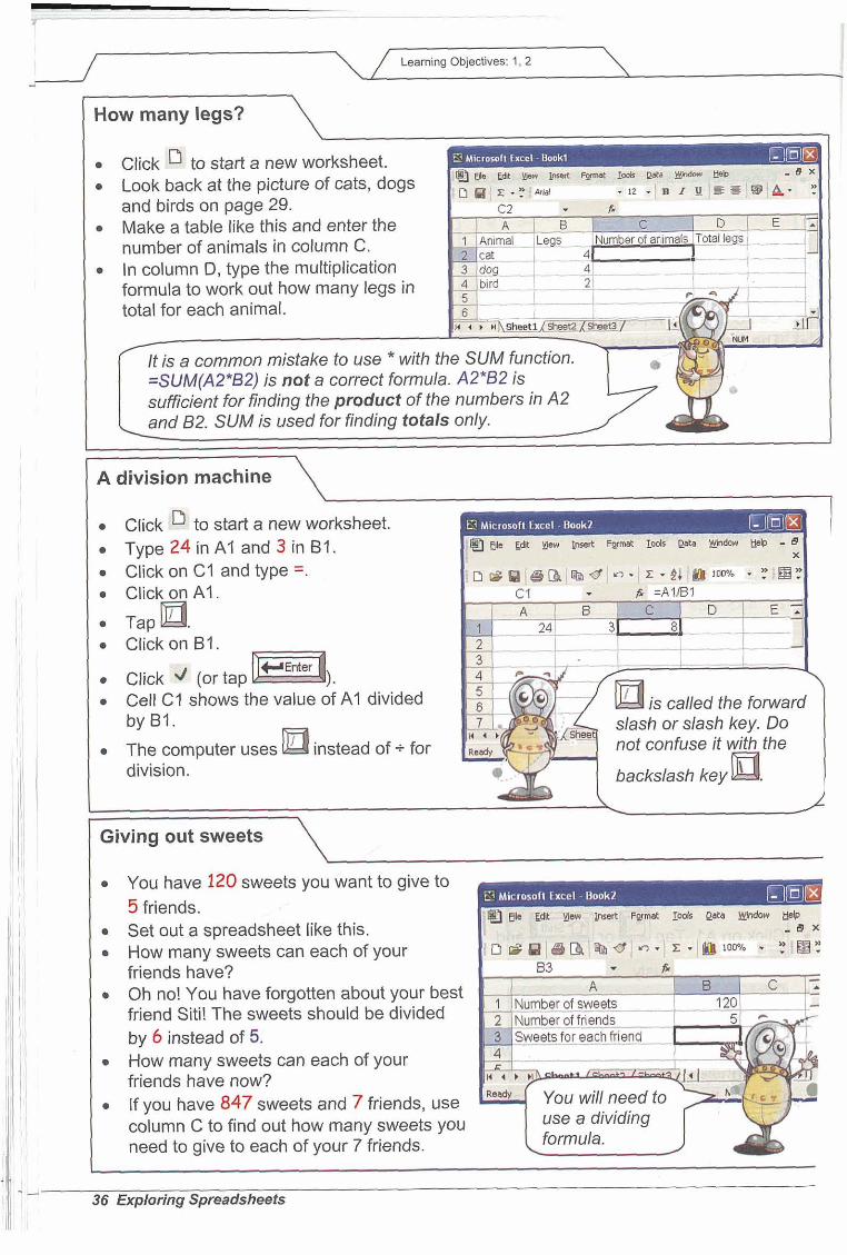
How many legs? - ~

Click !.& to start a new worksheet. Look back at the picture of cats, dogs and birds on page 29. Make a table like this and enter the number of animals in column C. In column D, type the multiplication formula to work out how many legs in total for each animal.

is a common mistake to use *with the SUM function. =SUM(A2*B2) is not a correct formula. A2*B2 is sufficient for finding the product of the numbers in A2

A division machine I

Microroll Excel B o o k ? u@l ~ . . .. . ...

-- - ~

Click 14 to start a new worksheet. Type24inAl and3inBl . Click on C1 and type =. Click on A l .

Cell C1 shows the value of A1 divided slash or slash key. Do

The computer uses instead of + for

Giving out sweets

Ll Microroll ixccl Uook7 lz You have 120 sweets you want to give to 5 friends. Set outa spreadsheet like this. How many sweets can each of your friends have? Oh no! You have forgotten about your best friend Siti! The sweets should be divided by 6 instead of 5. How many sweets can each of your friends have now? If you have 847 sweets and 7 friends, use column C to find out how many sweets you need to give to each of your 7 friends.

J 36 Exploring Spreidsheets


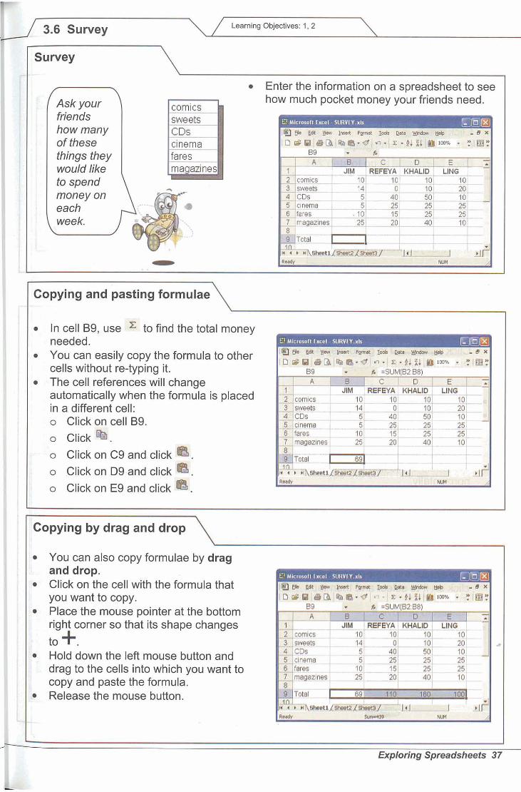
Survey

I Ask your friends how many of these things they would like to spend

Enter the information on a spreadsheet to see I ~w much pocket money your friends need.

I Total 1

L I

Copying and pasting formulae

In cell B9, use i,g to find the total money needed. You can easily copy the formula to other cells without re-typing it. The cell references will change automatically when the formula is placed in a different cell: o Click on cell B9. 0 Click ',@, o Click on C9 and click !.&. o .Click on D9 and click IR. o Click on E9 and click m.

i 'Copying by drag and drop

You can also copy formulae by drag and drop. Click on the cell with the formula that you want to copy. Place the mouse pointer at the bottom right corner so that its shape changes

to +. Hold down the left mouse button and drag to the cells into which you want to copy and paste the formula. Release the mouse button.

I Expforing Spreadsheets 37

Learning Objective: 3 / 3.7 Drawing graphs

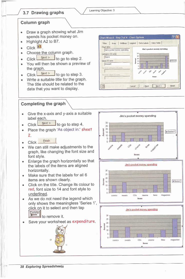
Column graph

Draw a grakh showing what Jim spends his pocket money on. Highlight A2 to B7. Click.:-@

Choose the column graph.

EEl to go to step 2. Click You will then be shown a preview of

the gr*l to go to step 3, Click Write a suitable title for the graph. . . . . - - . . , The title should be related to the data that you want to display.

Completing the graph

Give the x-axis and y-axis a suitable label each.

Click *~=,??%,: I to go to step 4.

Place the graph 'As object in:' sheet 2.

, , . , Click -!- -

We can still make adjustments to the @@ / fie a&@ e@ &@ graph, like changing the font size and font style. Enlarge the graph horizontally so that the labels of the items are aligned horizontally. 11

Make sure that the labels for all 6 25

items are shown clearly. - m E

15

Click on the title. Change its colour to 4 ,, red, font size to 14 and font style to 5

underlined. 0 cornnu m e t e CDs cnsms f s r e rnsgannss

As we do not need the legend which I,.",.

only shows the meaningless 'Series l', click on it to select and then tap pq

to remove it. Save your worksheet as expenditure.

C0.r. me43 CO. 011em b W " w a r n I,.,", . . -


Learning Objective: 3

Pie chart \

Instead of a column or bar chart, you can also use a pie chart to display the information. Go back to sheet 1 and highlight the same data, A2 to B7.

Click m. Choose Pie for Chart type. Click the middle type of the first row of the Chart sub-type to select a 3D pie chart.

0 Click ' .'( to proceed to step 2.

Steps 2 and 3 \ layed in step 2.

to proceed to step Chart Wirdrd Step 3 af 4 - C l w r t Options

Type the chart title as Jim's pocket money spending.

I Data labels \ Click ,I**J to open the data I labels folder. Check on Percentage and Show leader lines.

click to proceed to step 4.

If you show the Category name, then do not show

....

Exploring Spreadsheets I


p~ ~

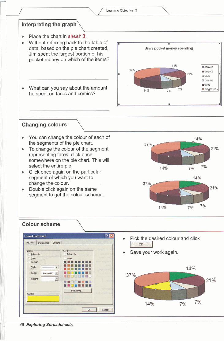
Interpreting the graph\ \

Place the chart in sheet 3. Without referring back to the table of data, based on the pie chart created, Jim spent the largest portion of his pocket money on which of the items?

What can you say about the amount he spent on fares and comics?

I Changing colours \ You can change the colour of each of the segments of the pie chart. To change the colour of the segment representing fares, click once somewhere on the pie chart. This will select the entire pie. Click once again on the particular segment of which you want to change the colour. Double click again on the same segment to get the colour scheme.

I Colour scheme \ Pick the desired colour and click

La Save your work again.



More graphs \ Draw a column chart to show Khalid's weekly expenditure. First highlight the items comics, 11 Ei~-~m~a.g;li~er, . m:il .. sweets, etc.

Hold down and highlight the data I - - for Khalid.

Click and choose a 3-D column graph. Write a suitable Chart title and label the x- and y-axes accordingly. Uncheck Show legend. In step 4, place the chart 'As new sheet:' Khalid. Save your worksheet using the same file name. . . . - . . -. . . . - .

Print a copy of this graph and glue it in the soace below. ~ - - 8 ~ - - - - - -

Draw similar charts for Refeya and " 1 - " F',> "7 ; , - .& *,:>& - A.-UA ... -a * a - . f-?&pi -*e"jl.y p q l

Ling. .,.." ,...; .. P. .. ..:. . 2 . . . .

Do you know why the graph for Refeya does .... not show any column for

I sweets? I

Glue your column chart here. It is all right for you to cover me.

.

Exploring Spreadsheets 4:


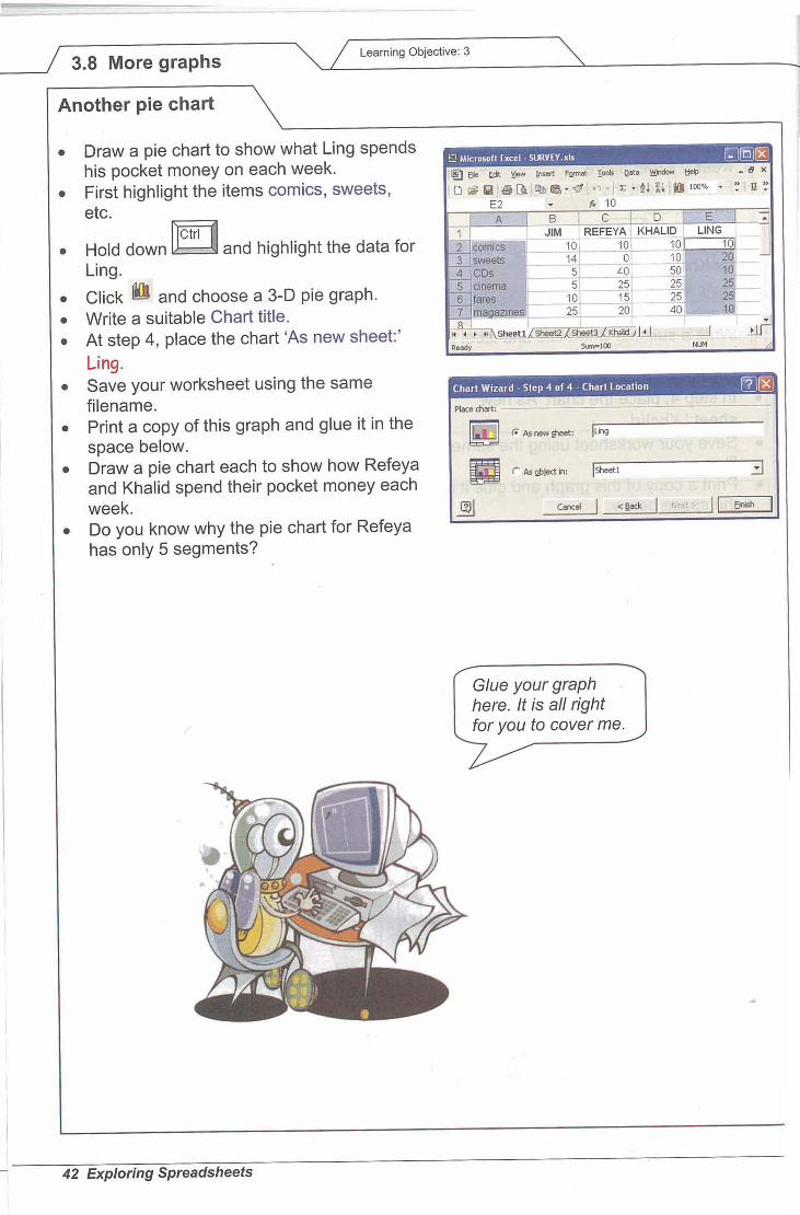
Another pie chart / I

Draw a pie chart to show what Ling spends his pocket money on each week. First highlight the items comics, sweets, etc.

old down and highlight the data for Ling. .

Click @ and choose a 3-D pie graph. Write a suitable Chart title. At step 4, place the chart 'As new sheet:'

Glue your graph here. It is all right for vou to cover me.

I


Ling. Save your worksheet using the same filename. Print a copy of this graph and glue it in the space below. Draw a pie chart each to show how Refeya and Khalid spend their pocket money each week. Do you know why the pie chart for Refeya has only 5 segments?

319 Completing data Learning Objectives: 4, 5

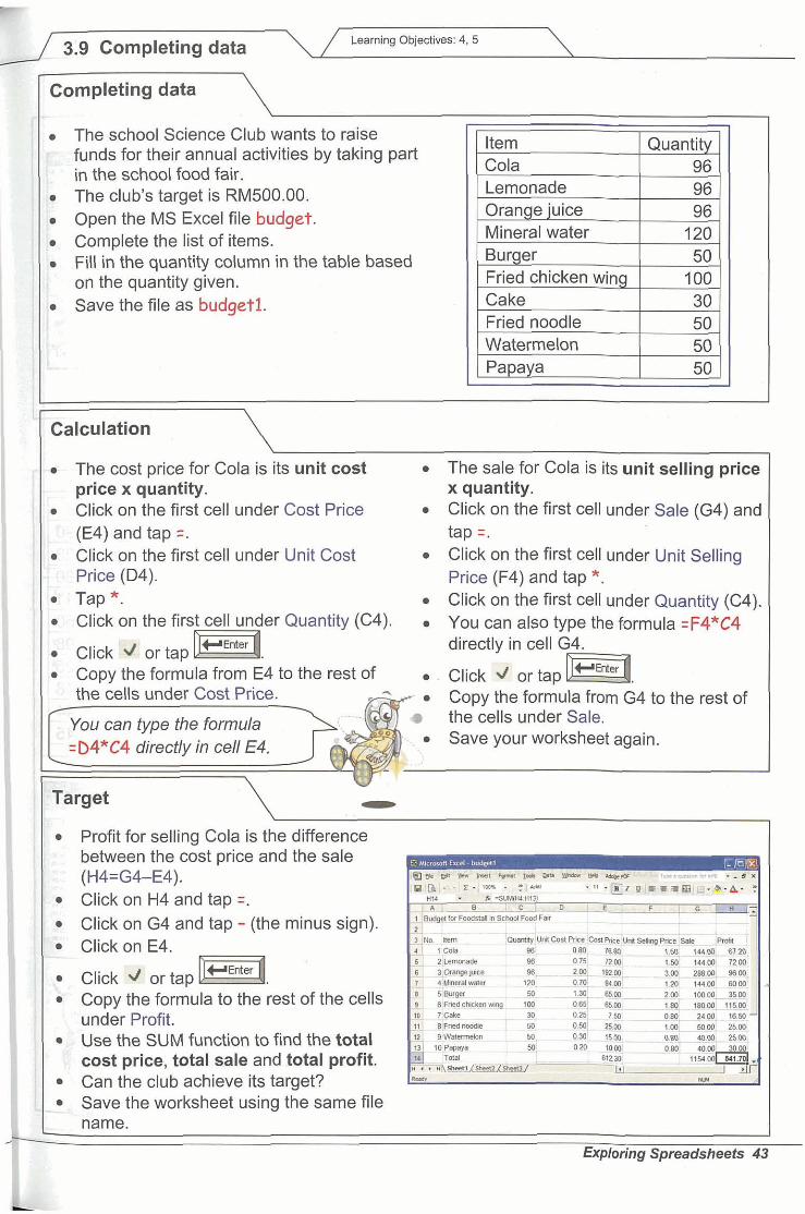
I I I Profit for sellina Cola is t\he difference

IT %

.,$ ,

-

between the cost price and the sale (H4=G4-E4). Click on H4 and tap =. Click on G4 and tap - (the minus sign).

- price x quantity. ' , a Click on the first cell under Cost Price Click on the first cell under Sale (G4) and

Click on the first cell under Unit Selling Price (F4) and tap *. Click on the first cell under Quantity (C4).

Copy the formula from G4 to the rest of the cells under Sale.

Completing data

Click on E4.

Click 4 or taD p q ,

- The school Science Club wants to raise

r.;, funds for their annual activities by taking part i"' in the school food fair. I. I The club's target is RMf;OO.Ofl~ p Open the MS Excel file ! j* Complete the list of items. I. Fill in the quantity column in the table based

on the quantity given. ! 1. Save the file as budgetl.

' 1 1. i~

Copy the formula to the rest of the cells under Profit. Use the SUM function to find the total cost price, total sale and total profit. Can the club achieve its target?

IslPI.n.lr -I>- - :I? "1, ,..: ' *-:",,I

- '! .I@' .slk~~&~,@:*a. 1 . . B I - C I - I ~ T O I .E >,. .. F . ,.I. 0-

! tor F d m h Srhrm~c@Fa% -~. 1 1 ,

Item Cola Lemonade Orange juice Mineral water Burger Fried chicken wing Cake Fried noodle Watermelon Papaya

1 1 1 Save the worksheet using the same file I

Quantity 96 96 96

120 50

100 30 50 50 50

name. \-.


Learning Objectives: 4, 5 3.10 What if \

ii / Change data

It was found that the unit cost prices for some of the items were wrongly quoted. The correct unit cost prices are as follow: o Burger - RMI .50 0 Fried chicken wing - RM0.85 With these changes in price, do you think the club can still achieve the target of RM500? Adjust the unit cost prices as above. Save your adjusted spreadsheet as budget2 Was your prediction correct?

Actual sale

During the actual fair, what if some of the items were not completely sold? Do you think the club can still reach the

target of RM500?

Insert a column in between columns E on and F: select column E. Click . . -

. - the menu bar, then select Enter the column head as Quantity Sold. Enter the quantities sold in this new column F. You will need to change the formula for Sale. The formula for Sale for Cola is now quantity sold x unit selling price. Copy this formula to the rest of the cells in column H. Use the SUM function to find the total actual sale. Was your prediction correct?

Draw a column chart to show the profit for each item. Place the chart below the spreadsheet. Save your work as budget3 Based on the graph, which item has the highest profit?


3.11 Evide Learntng Objectives 4, 5 -

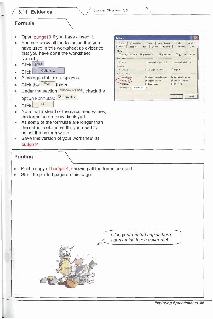
Formula \ Open budget3 if you have closed it. You can show all the formulae that you have used in this worksheet as evidence that you have done the worksheet correctlv.

A dialogue table is displayed. : ................... __5

Click the ..... !.!% .... @folder. Under the section Bindow check the

option Formulas: FO~mu'as . Click I, Note that instead of the calculated values, the formulae are now displayed. As some of the formulae are longer than the default column width, you need to adjust the column width. Save this version of your worksheet as budget4

Printing

Print a copy of budget4, showing all the formulae used. Glue the printed page on this page.


Glue the printout on this page as evidence of your hard work.


module 3 exploring spreadsheets - pbworksteachit2009.pbworks.com/f/exploring+spreadsheets.pdf ·...

Documents