Module 8: Estimating Genetic Variances

– Nested design

–GCA, SCA

– Diallel

PBG 650 Advanced Plant Breeding

Nested design

• Also called– North Carolina Design 1

– Hierarchical design

• Two types of families

– Half sibs (male groups)

– Full-sibs (females/males)

Males Females

1

2...m

1234

5678

.

.f

Nested design – one location

Source df MS Expected Mean Square

Blocks r-1 MSR

Males m-1 MSM

Females/males m(f-1) MSF

Error (r-1)(mf-1) MSE

2

M

2

M/F

2

e rfr 2

M/F

2

e r 2

e

Linear Model Yijk= + Bi + Mj + Fk(j) + eijk

rf

MSMS FM2

M

r

MSMS eF2

M/F

F

Mmales

MS

MSF

e

FM/F

MS

MSF

• Might also have sets and multiple environments

See Bernardo, pg 164, for ANOVA with sets and environments

Variance components from the nested design

2

M

2

A

2

A412

M

2

Halfsibs

F1

4

(if the parents are not inbred)

2M

2M/F2

2

D

2

D412

A412

Halfsibs

2

Fullsibs

2

M/F

2

M/F

2

M

2

Fullsibs

)F1(

4

(if the parents are not inbred)

Expected Mean Squares in SAS

Source Type III Expected Mean SquareLoc Var(Error) + 3 Var(Loc*Cultivar) + 7 Var(Rep(Loc)) + 21 Var(Loc) Rep(Loc) Var(Error) + 7 Var(Rep(Loc))Cultivar Var(Error) + 3 Var(Loc*Cultivar) + Q(Cultivar)Loc*Cultivar Var(Error) + 3 Var(Loc*Cultivar)

Proc GLM;Class Loc Rep Cultivar;Model Yield=Loc Rep(Loc) Cultivar Loc*Cultivar;Random Loc Rep(Loc) Loc*Cultivar/Test;Run;

• Random statement generates expected mean squares

• Test option obtains appropriate F tests for the model specified

• In the example below, cultivars are fixed, all other effects are random

controversial (could be dropped)

• Proc Mixed may give better estimates of variance components

fixed effect

2

Loc

Combining Ability

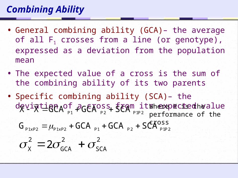
• General combining ability (GCA)– the average of all F1 crosses from a line (or genotype), expressed as a deviation from the population mean

• The expected value of a cross is the sum of the combining ability of its two parents

• Specific combining ability (SCA)– the deviation of a cross from its expected value

2P1P2P1P SCAGCAGCAXX Where X is the performance of the cross

2

SCA

2

GCA

2

X 2 2P1P2P1P2xP1P2xP1P SCAGCAGCAG

Estimation of combining ability

GCA

• polycross method - allow all lines to intermate naturally

• top crossing - a line is crossed to a random sample of plants from a reference population

GCA and SCA

• Factorial design (NC Design II) – a group of ‘male’ parents is crossed to a group of ‘female’ parents– requires mxf crosses (e.g. 5x5=25)

– can be applied to two heterotic populations

• Diallel – all possible crosses among a set of parents– n(n-1)/2 possible crosses without parents or reciprocals

(e.g. 10x9/2=45)

Variations on the Diallel

• Type of cross-classified design

• With or without the parents

• With or without reciprocal crosses– bulk seed from both parents if maternal effects are not important

• Genotypes may be random or fixed– For random model, need many parents to adequately sample the

population

• Large number of crosses!– Can be divided into sets

– Partial diallels can be conducted

• If parents are inbred, can make paired row crosses to obtain more seed

Hallauer, Carena, and Miranda (2010) pg 119-138

Griffing’s Methods (Diallels)

• Method 1– all possible crosses, including selfs

• Method 2– no reciprocals

• Method 3– no parents

• Method 4– no parents or reciprocals

– most common, because parents often inbred and less vigorous

For each Method, genotypes may be Model I = FixedModel II = Random

Diallel crossing

Parent A B C D ……. N Mean

A a+a a+b a+c a+d a+n a

B b+b b+c b+d b+n b

C c+c c+d c+n c

D d+d d+n d

N n+n n

…..

…..

Diallel analysis

Random model

• Usually does not include parents and reciprocals

• Can be divided into sets

Griffing (1956) is classic reference

Source df MS Expected Mean Square

Blocks r-1

Crosses [n(n-1)/2] -1 MS2

GCA n-1 MS21

SCA n(n-3)/2 MS22

Error (r-1){[n(n-1)/2] -1} MS1

2

C

2

e r 2

GCA

2

SCA

2

e )n(rr 2

2

e

2

SCA

2

e r

)2n(r

MSMS 22212

GCA

r

MSMS 1222

SCA

Genetic variances from random model

2

GCA

2

A

2

AHS

2

GCA

F1

4

4

F1Cov

2

SCA2

2

D

2

D

2

HSFS

2

SCA

)F1(

4

4

)F1(Cov2Cov

2f

MS

k

2)ˆ(Var

g

2

g

2

2

g

k=coefficient of MSfg=df of the mean square

General form for variance of a variance component

Fixed model

• GCA effects

• SCA effects

..X2.nX)n(n

g ii2

1

..X)n)(n(

2.X.X

)n(nXs

212

1jiijji

2

ei

2

)2n(n

1n)g(

2

eij

2

1n

3n)s(

Advantage: first order effects (means)are estimated with greater precisionthan variances

Lattice designs are useful

Diallel analysis with parents

Source df

Blocks r-1

Entries [n(n+1)/2]-1

Parents n-1

Parents vs crosses 1

Crosses [n(n-1)/2]-1

GCA n-1

SCA n(n-3)/2

Error (r-1){[n(n+1)/2] -1}

Source df

Blocks r-1

Entries [n(n+1)/2]-1

Varieties n-1

Heterosis n(n-1)/2

Average

1

Variety n -1

Specific n(n-3)/2

Error (r-1){[n(n+1)/2] -1}

Gardner-Eberhart Analysis II

• Gardner-Eberhart partitioning of Sums of Squares is non-orthogonal• Fit model sequentially

Factorial Mating Design

1 2 3 4 1 2 3 4

Parents(females)

Parents(females)

1 ….. X12 X13 X14 5 X15 X25 X35 X45

2 ….. X23 X24 6 X16 X26 X36 X46

3 ….. X34 7 X17 X27 X37 X47

4 ….. 8 X18 X28 X38 X48

Parents (males) Parents (males)Diallel Factorial (Design II)

Parents Diallel Factorial

4 6 4

6 15 9

10 45 25

20 190 100

100 4950 2500

n n(n-1)/2 n2/4

General formula for covariance of relatives

2D

2ArCov

A B C D

X Y

r = 2XY

= ACBD + ADBC

Extended to include epistasis:

... 2DD

22AD

2AA

22D

2A rrrCov

Epistatic Variance

• Often assumed to be absent, but could bias estimates of A

2 and D2 upwards

• Estimation requires more complex mating designs

• Expected to be smaller than A2 and D

2, so larger experiments are needed for adequate precision

• Coefficients are correlated with those for A2 and D

2, which leads to multicollinearity problems

• For most crops, experimental estimates of epistatic variance have been small

Example of mating design to estimate epistatic variance

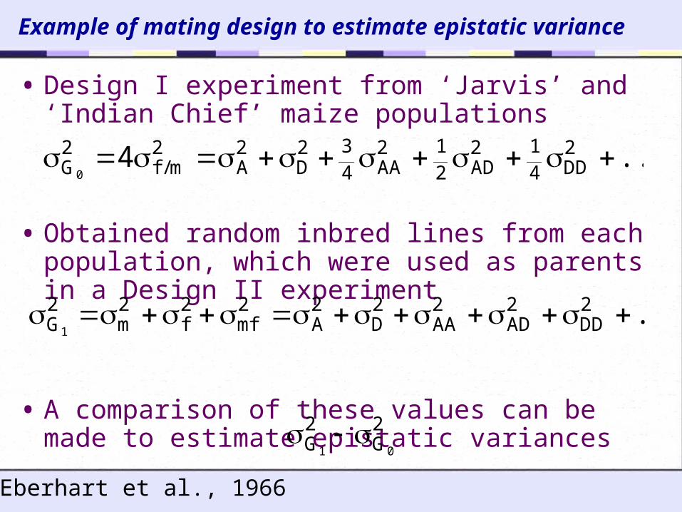
• Design I experiment from ‘Jarvis’ and ‘Indian Chief’ maize populations

• Obtained random inbred lines from each population, which were used as parents in a Design II experiment

• A comparison of these values can be made to estimate epistatic variances

Eberhart et al., 1966

.../ 2DD4

12AD2

12AA4

32D

2A

2mf

2G 4

0

... 2DD

2AD

2AA

2D

2A

2mf

2f

2m

2G1

2G

2G 01

Precision of variance components

• Minimum of 50-100 progeny to adequately sample population (Bernardo’s advice, some would say more!)

• Large numbers of progeny do not guarantee precise estimates of variance

• Confidence intervals can be determined for estimates of variance (sets lower and upper bounds)

• It’s possible in practice to obtain negative estimates of variance components, but they are theoretically impossible

– large error variance

– true estimate of genetic variance is close to zero

– Report as zero? (may lead to bias when results are compiled across many experiments)

See Bernardo, pg 166, for further details on confidence intervals

Resampling methods

• Confidence interval calculations assume that the underlying distribution is normal. Work best for balanced data.

• Resampling methods are useful when– underlying distributions are unknown or are not normal

– we don’t know how to estimate the confidence interval

• Examples– Bootstrap – resampling with replacement

– Jackknife – systematically delete data points

– Permutation test – data scrambling• only works when there are two or more types of families