module 9 topic 9 introduction to matrices integration · antiderivatives and inde nite integrals...
TRANSCRIPT

MathsTrack
MATHEMATICS LEARNING SERVICE
Centre for Learning and Professional Development
Level 1, Schulz Building (G3 on campus map)
TEL 8303 5862 | FAX 8303 3553 | [email protected]
www.adelaide.edu.au/clpd/maths/
Module 9
Introduction to Matrices
Income = Tickets ! Price
=
�
250 100
350 150
!
" #
$
% &
25 30 35
20 15 10
!
" #
$
% &
=
�
8,250 9,000 9,750
11,750 12,750 13,750
!
" #
$
% &
(NOTE Feb 2013: This is the old version of MathsTrack.New books will be created during 2013 and 2014)
Topic 9
Integration
-�x
y = f(x)
y = g(x)
a b
Area
Area =
∫ b
a
f(x)− g(x) dx = [F (x)−G(x)]ba
MATHS LEARNING CENTRELevel 3, Hub Central, North Terrace Campus, The University of AdelaideTEL 8313 5862 — FAX 8313 7034 — [email protected]/mathslearning/

This Topic . . .
The topic has 2 chapters:
Chapter 1 introduces integration which together with differentiation are parts ofthe branch of mathematics called Calculus.
The chapter begins by asking the question: Given the rate of change of aquantity, how can we find the quantity? This question is related to the problemof finding the area of the region between a curve and the horizontal axis. Upperand lower rectangles are used to approximate this region.
The definite integral is introduced together with its properties.
Chapter 2 introduces the Fundamental Theorem of Calculus. This central theoremlinks integration to differentiation and enables integrals to be evaluated by‘reverse’ differentiation.
Antiderivatives and indefinite integrals are introduced. Standard integrals areused to used to integrate more complex functions. The substitution methodis used to simplify the integration of composite functions.
Selected applications include calculation of the exact area between two curvesand of net change in quantities.
The topic uses the standard derivatives and methods of differentiation introduced inTopic 6.
Auhor: Dr Paul Andrew January 2008
Edited by: Geoff Coates Printed: February 24, 2013
i

Contents
1 Integrals 1
1.1 Introduction . . . . . . . . . . . . . . . . . . . . . . . . . . . . . . . . 1
1.2 Area under a curve . . . . . . . . . . . . . . . . . . . . . . . . . . . . 6
1.3 The definite integral . . . . . . . . . . . . . . . . . . . . . . . . . . . 10
1.4 Properties of the definite integral . . . . . . . . . . . . . . . . . . . . 14
1.4.1 Additive Properties . . . . . . . . . . . . . . . . . . . . . . . . 14
1.4.2 Linear Properties . . . . . . . . . . . . . . . . . . . . . . . . . 15
2 Integration 17
2.1 Fundamental Theorem of Calculus . . . . . . . . . . . . . . . . . . . 17
2.2 Integration . . . . . . . . . . . . . . . . . . . . . . . . . . . . . . . . . 20
2.2.1 Antiderivatives and indefinite integrals . . . . . . . . . . . . . 20
2.2.2 Methods . . . . . . . . . . . . . . . . . . . . . . . . . . . . . . 23
2.2.3 Selected Applications . . . . . . . . . . . . . . . . . . . . . . . 36
A Summation Notation 47
B Justification for the Fundamental Theorem 49
C Answers 52
ii

Chapter 1
Integrals
1.1 Introduction
Differentiation was concerned with the question:
Given a quantity, how can we find its rate of change?
If we know the volume of water entering a dam as a function of time, we can usedifferentiation to find the rate at which the dam is filled.
This topic introduces integration, which is concerned with the question:
Given the rate of change of a quantity, how can we find the quantity?
If we know the rate at which a dam is filled, we use integration to find the volumeof water entering the dam as a function of time.
Differentiation and integration are parts of Calculus.i
Example
constantflow
A dam is filled from a creek with a constant flow of 2000 litres/min. This isshown on the flow-time graph below.
6
flow (litres/min)
2,000
-0 time (min)
iCalculus is a branch of mathematics that includes the study of limits, differentiation, inte-gration and infinite series, and has widespread applications in science and engineering. The wordcalculus was introduced in the mid 17th century from Latin, and means ‘a small stone used forcounting’.
1

2 CHAPTER 1. INTEGRALS
As the flow is constant, the volume of water flowing into the dam after tminutes is:
volume = flow× time
= 2000× t= 2000 t litres
You can see that the volume of water entering the dam is the area under theflow-time graph from 0 to t minutes:
6
flow (litres/min)
2,000
-0 t time (min)
Example
changingflow
Suppose instead that the flow of water entering the dam changed at the rate2000− 100t litres/min after t minutes. The flow-time graph would then be:
6
flow (litres/min)
HHHHH
HHHHHH
HHH
2,000
-0 20 time (min)
We can estimate the volume of water entering the dam in 20 minutes bysubdividing the interval [0, 20] on the x-axis into four equal parts:
6
flow (litres/min)
HHHHHH
HHHHHH
HH
2,000
-0 5 10 15 20 time (min)

1.1. INTRODUCTION 3
You can see that the area of the upper rectangle above interval [ 0, 5 ]
height × width = 2000× 5
= 100, 000
is an upper estimate of the volume of water flowing into the dam for 0 ≤ t ≤ 5,and that the area of the lower rectangle
height × width = (2000− 100× 5)× 5
= 75, 000
is a lower estimate of the volume of water flowing into the dam for 0 ≤ t ≤ 5.
The sum of the areas of the four upper rectangles gives an upper estimate ofthe total volume water flowing into the dam for the 20 minutes:
2000× 5 + (2000− 100× 5)× 5 + (2000− 100× 10)× 5 + (2000− 100× 15)× 5
= 25, 000 litres
and the sum of the areas of the lower rectangles give a lower estimate of thetotal volume:
(2000− 100× 5)× 5 + (2000− 100× 10)× 5 + (2000− 100× 15)× 5 + 0
= 15, 000 litres
. . . the volume of water entering the dam is between 15, 000 and 25, 000 litres.
This estimate can be improved by taking finer subdivisions of interval [ 0, 20 ].
6
flow (litres/min)
HHHHHHH
HHHHHHH
2,000
-0 5 10 15 20 time (min)
With eight subdivisions, the upper and lower estimates are 17, 500 and 22, 500.
As smaller subdivisions are taken, you can see that the sum of the areas ofthe upper and lower rectangles become closer to each other and that both sumsbecome very close to the area under the flow-time curve between t = 0 andt = 20.
4 CHAPTER 1. INTEGRALS
6
flow (litres/min)
HHHHHH
HHHHHH
HH
2,000
-0 20 time (min)
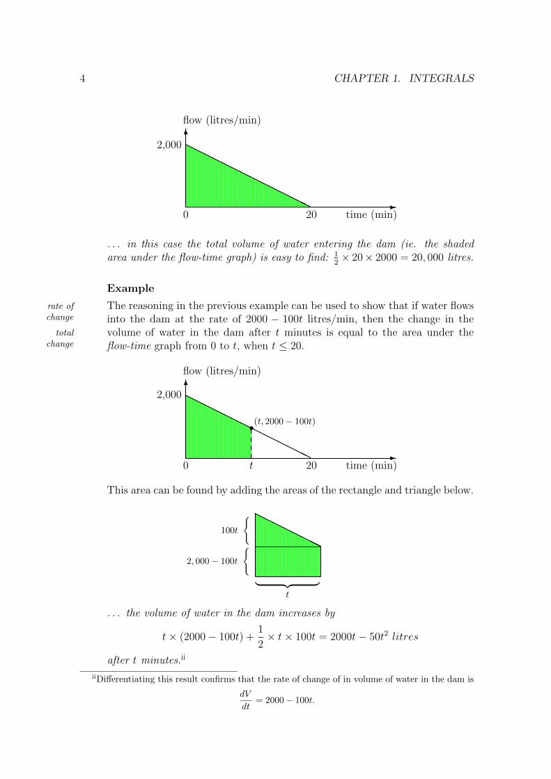
. . . in this case the total volume of water entering the dam (ie. the shadedarea under the flow-time graph) is easy to find: 1
2× 20× 2000 = 20, 000 litres.
Example
rate ofchange
totalchange
The reasoning in the previous example can be used to show that if water flowsinto the dam at the rate of 2000 − 100t litres/min, then the change in thevolume of water in the dam after t minutes is equal to the area under theflow-time graph from 0 to t, when t ≤ 20.
6
flow (litres/min)
HHHHH
HHHHHH
HHH
2,000
-
(t, 2000− 100t)
0 t 20 time (min)
s
This area can be found by adding the areas of the rectangle and triangle below.
HHHH
HHHH
︸ ︷︷ ︸t
100t
{
2, 000− 100t
{
. . . the volume of water in the dam increases by
t× (2000− 100t) +1
2× t× 100t = 2000t− 50t2 litres
after t minutes.ii
iiDifferentiating this result confirms that the rate of change of in volume of water in the dam is
dV
dt= 2000− 100t.

1.1. INTRODUCTION 5
Exercise 1.1
1. Rainwater flowed into a 1,000 litre tank at a constant rate of 10 litres/min.
(a) Draw a graph of the constant flow f(t) into the tank for t ≥ 0 minutes.
(b) Calculate the total volume of the water flowing into the tank after tminutes.
(c) Draw a graph of the volume V (t) of water in the tank for 0 ≤ t ≤ 60, ifthe tank contained 100 litres before the rain began.
(d) Interprete the gradient of the line in (c).
2. At time t = 0, a car began travelling up a hill with a velocityiii of
v(t) = 30− 0.5t m/s,
where t is measured in seconds.
(a) Draw a graph of the velocity v(t) of the car for 0 ≤ t ≤ 60 seconds.
(b) Calculate the distance travelled by the car after 60 seconds.
(c) Calculate the distance s(t) travelled by the car after t seconds.
3. Sketch the parabola y = 1− x2 for 0 ≤ x ≤ 1.
Estimate the area between the parabola and the x-axis for 0 ≤ x ≤ 1 by:
i. subdividing the interval [ 0, 1 ] into five equal parts.
ii. constructing upper and lower rectangles on each subinterval to obtainupper and lower estimates of the area under the parabola and above eachsubinterval.
iii. summing of the areas of the upper and lower rectangles.
iiivelocity = rate of change of distance with time.

6 CHAPTER 1. INTEGRALS
1.2 Area under a curve
In the previous section we discovered that the answer to the question:
Given the rate of change of a quantity, how can we find the quantity?
was found by examining the area under the rate of change graph.
We can calculate the exact area under some curves, but for others we cannot andin these cases we need to estimate the area.iv
If f(x) is a positive continuous function on [ a, b ], then we can estimate the areabetween the curve and the x-axis from x = a to x = b by using upper and lowerrectangles.
Example
upperrectangles
lowerrectangles
Consider the function f(x) = x2 and the region between the graph of f(x) andthe x-axis, bounded by the vertical lines x = 1 and x = 4.
625
-0 1 2 3 4 5
We can estimate the area A of this region by subdividing the interval [ 1, 4 ]into three equal intervals of length 1, and then using upper rectangles on eachsubinterval to estimate the area under the curve.
Upper rectangles are rectangles with height equal to the maximum value of afunction on a subinterval.
625
-0 1 2 3 4 5
ivThis will be discussed in more detail later.

1.2. AREA UNDER A CURVE 7
The sum AU of the areas of the upper rectangles
AU = 1× f(2) + 1× f(3) + 1× f(4)
= 1× 4 + 1× 9 + 1× 16
= 29
is an upper estimate of area A.
We can find a lower estimate for A by using lower rectangles.
Lower rectangles are rectangles with height equal to the minimum value of afunction on a subinterval.
625
-0 1 2 3 4 5
The sum AL of the areas of the lower rectangles
AL = 1× f(1) + 1× f(2) + 1× f(3)
= 1× 1 + 1× 2 + 1× 9
= 12
is an lower estimate of area A.
This shows that area A is between 12 and 29 unit 2.
We can get a better estimate of A by taking smaller subintervals.
For example, if [ 1, 4 ] was divided into 6 equal parts of length 0.5, then thesum of the areas of the upper rectangles would be:
AU = 0.5× f(1.5) + 0.5× f(2) + 0.5× f(2.5) + 0.5× f(3)
+ 0.5× f(3.5) + 0.5× f(4)
= 0.5× 1.52 + 0.5× 22 + 0.5× 2.52 + 0.5× 32 + 0.5× 3.52 + 0.5× 42
= 24.875 ,
and the sum of the areas of the lower rectangles would be:
AL = 0.5× f(1) + 0.5× f(1.5) + 0.5× f(2) + 0.5× f(2.5)
+ 0.5× f(3) + 0.5× f(3.5)
= 0.5× 12 + 0.5× 1.52 + 0.5× 22 + 0.5× 2.52 + 0.5× 32 + 0.5× 3.52
= 17.375 .

8 CHAPTER 1. INTEGRALS
. . . showing 17.375 ≤ A ≤ 24.875.
As further subdivisions are taken, the difference between AU and AL becomessmaller and each become closer to the area A (= 21 unit 2).
It is easy to estimate the difference AU − AL when f(x) is either an increasingfunction or a decreasing function.
Example (continued)
AU −AL As f(x) = x2 is an increasing function, the diagram below shows that thedifference in areas AU − AL is equal to the area of a rectangle with:
• width = width of subinterval
• height = height of largest upper rectangle− height of smallest lower rectangle
625
-0 1 2 3 4 5
This observation can be used to calculate how small subintervals need be inorder to estimate area A with a predetermined precision.
For example, if we wish to estimate A to within 0.1 unit2, then we need to usesubintervals of width w where
w × (16− 1) ≤ 0.1

1.2. AREA UNDER A CURVE 9
Exercise 1.2
1. Sketch the parabola y = 1− x2 for 0 ≤ x ≤ 1.
(a) Estimate the area between the parabola and the x-axis for 0 ≤ x ≤ 1 by:
i. subdividing the interval [ 0, 1 ] into two equal parts.
ii. constructing upper and lower rectangles for each subinterval.
iii. summing the areas of the upper and lower rectangles.
(b) How many subintervals do you need to estimate the area to within 0.1unit2 ?
2. Sketch the parabola y = 1− x2 for −1 ≤ x ≤ 1.
Estimate the area between the parabola and the x-axis by:
i. subdividing the interval [−1, 1 ] into four equal parts.
ii. constructing upper and lower rectangles for each subinterval.
iii. summing the areas of the upper and lower rectangles.

10 CHAPTER 1. INTEGRALS
1.3 The definite integral
Suppose that f(x) is a positive continuous function for a ≤ x ≤ b, and that theinterval [ a, b ] is divided into n equal parts by the points x0, x1, . . . , xn, with a = x0and b = xn.
The area A between the curve y = f(x) and the x-axis from x = a to x = b can beestimated by constructing rectangles of heights f(x0), f(x1), . . . , f(xn−1) on eachof the intervals [ x0, x1 ], [ x1, x2 ], . . . , [xn−1, xn ] as in the diagram below.
y = f(x)6y
-xa x1 x2 x3 xn−2 xn−1 b
x0 xn
. . . . . .
The sum of the areas of these rectangles is equal to v
f(x0)∆x+ f(x1)∆x+ f(x2)∆x+ · · ·+ f(xn−1)∆x =n−1∑i=0
f(xi)∆x
where ∆x =b− an
.
As each rectangle is between the upper and lower rectangles on the same subinterval,you can see that
n−1∑i=0
f(xi)∆x→ A as n→∞ .
The limit
limn→∞
n−1∑i=0
f(x) ∆x
is represented by ∫ b
a
f(x) dx
which is read aloud as ‘the integral from a to b of f(x) dee x’.vi
vSee Appendix A.viThe verb to integrate means to form into one whole, and integral is the whole obtained after
integration.

1.3. THE DEFINITE INTEGRAL 11
In this form :
• the limit replaces the ‘∑
’ with an elongated S, ‘
∫’ , called the integral
symbol.
• the ∆x is replaced by dx
• the values at the top and bottom of the integral symbol are the boundariesof the region between the curve y = f(x) and the x-axis. They are called theupper and lower limits of the integral.
This integral is called a definite integral as its upper and lower limits are given. Wewill consider indefinite integrals in the next chapter.
If f(x) is a positive continuous function for a ≤ x ≤ b, then the area betweenthe curve y = f(x) and the x-axis from x = a to x = b is represented bythe definite integral: ∫ b
a
f(x) dx
Note: It is easier to work with a sum like
f(x0)∆x + f(x1)∆x + f(x2)∆x + · · ·+ f(xn−1)∆x =n−1∑i=0
f(xi)∆x ,
than it is with sums of areas of upper and lower rectangles, as the heights of the rectangles
have a clear pattern.
We need to investigate the definite integral further . . . .
Suppose that f(x) is a negative continuous function for a ≤ x ≤ b, and that theinterval [ a, b ] is divided into n equal parts by the points x0, x1, . . . , xn, with a = x0and b = xn.
The area A between the curve y = f(x) and the x-axis from x = a to x = b can beestimated using rectangles of heights −f(x0), −f(x1), . . . , −f(xn−1) on each of theintervals [x0, x1 ], [ x1, x2 ], . . . , [xn−1, xn ], as in the diagram below.
y = f(x)
6
?
y
-x
a x1 x2 x3 xn−2 xn−1 b
x0 xn
−→height
−f(x0)
u(x0, f(x0))
. . . . . .
12 CHAPTER 1. INTEGRALS
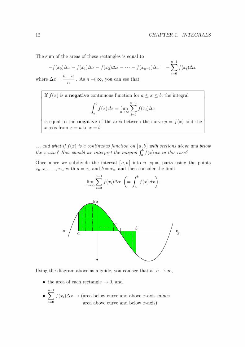
The sum of the areas of these rectangles is equal to
−f(x0)∆x− f(x1)∆x− f(x2)∆x− · · · − f(xn−1)∆x = −n−1∑i=0
f(xi)∆x
where ∆x =b− an
. As n→∞, you can see that
If f(x) is a negative continuous function for a ≤ x ≤ b, the integral∫ b
a
f(x) dx = limn→∞
n−1∑i=0
f(xi)∆x
is equal to the negative of the area between the curve y = f(x) and thex-axis from x = a to x = b.
. . . and what if f(x) is a continuous function on [ a, b ] with sections above and below
the x-axis? How should we interpret the integral∫ baf(x) dx in this case?
Once more we subdivide the interval [ a, b ] into n equal parts using the pointsx0, x1, . . . , xn, with a = x0 and b = xn, and then consider the limit
limn→∞
n−1∑i=0
f(xi)∆x
(=
∫ b
a
f(x) dx
).
6
?
y
-�xa
b. . . . .
. . .
Using the diagram above as a guide, you can see that as n→∞,
• the area of each rectangle → 0, and
•n−1∑i=0
f(xi)∆x→ (area below curve and above x-axis minus
area above curve and below x-axis)

1.3. THE DEFINITE INTEGRAL 13
In general,
If f(x) is a continuous function for a ≤ x ≤ b, then∫ b
a
f(x) dx = limn→∞
n−1∑i=0
f(xi)∆x
is equal to the difference between
(a) the sum of the areas under f(x) and above the x-axis and
(b) the sum of the areas above f(x) and below the x-axis
for a ≤ x ≤ b.
Exercise 1.3
1. It is known that ∫ π/2
0
sin(x) dx = 1
Use the graph of sin x below to evaluate
(a)
∫ π
0
sin(x) dx
(b)
∫ 0
−πsin(x) dx
(c)
∫ 3π/2
0
sin(x) dx
-�x
6
?
y
−π 0 π 2π
2. Draw an appropriate graph and use it to evaluate∫ π
0
(1 + sin(x)) dx

14 CHAPTER 1. INTEGRALS
1.4 Properties of the definite integral
1.4.1 Additive Properties
The following properties are useful when evaluating integrals.
Property 1 (Additivity)
If f(x) is continuous on [ a, b ] and a < c < b, then∫ c
a
f(x) dx+
∫ b
c
f(x) dx =
∫ b
a
f(x) dx
This property is clearly true when f(x) is a positive continuous function on [ a, b ],as the area between the curve y = f(x) and the x-axis from x = a to x = b is equalto the sum of areas from x = a to x = c, and from x = c to x = b. It can also beconfirmed directly when f(x) takes negative values on [ a, b ].
Property 2 ∫ a
a
f(x) dxdef= 0
The original definition of the integral∫ baf(x) dx assumed that a < b. Property 2
is an extension of this definition to the case a = b.vii It is intuitively valid as arectangle with zero width has zero area.
Property 3
If f(x) is continuous on [ a, b ], then∫ a
b
f(x) dxdef= −
∫ b
a
f(x) dx
The original definition of the integral∫ baf(x) dx assumed that a < b. Property 3 is
an extension of this definition to the case a > b. It is consistent with properties 1and 2 as ∫ b
a
f(x) dx+
∫ a
b
f(x) dx =
∫ a
a
f(x) dx = 0
Observe that properties 2 and 3 show that there is no restriction on the numbers thatcan be used as upper and lower limits in integrals.
viiThe symboldef= means is defined as.

1.4. PROPERTIES OF THE DEFINITE INTEGRAL 15
1.4.2 Linear Properties
The following properties are used to rewrite integrals of complex functions in termsof integrals of simpler functions.
Property 1
If f(x) is continuous on [ a, b ] and k is a constant, then∫ b
a
kf(x) dx = k
∫ b
a
f(x) dx
This follows directly from the definition of an integral as
n−1∑i=0
kf(x)∆x = k
(n−1∑i=0
f(x)∆x
)
Property 2
If f(x) and g(x) are continuous on [ a, b ], then∫ b
a
(f(x) + g(x)) dx =
∫ b
a
f(x) dx+
∫ b
a
g(x) dx
This follows directly from the definition of an integral as
n−1∑i=0
(f(x) + g(x))∆x =n−1∑i=0
f(x)∆x+n−1∑i=0
g(x)∆x
Note: Properties 1 and 2 can be extended to any linear combinationviii of functions. If
• f(x), g(x), h(x), . . . are continuous on [ a, b ] and
• h, k, l, . . . are constants,
then∫ b
a(hf(x) + kg(x) + lh(x) + . . .) dx = h
∫ b
af(x) dx + k
∫ b
ag(x) dx + l
∫ b
ah(x) dx + . . .
viiiA linear combination of functions is a sum of multiples of the functions. Many mathematicalfunctions are constructed from linear combinations of simpler functions. For example, polynomialsare linear combinations of powers.

16 CHAPTER 1. INTEGRALS
Exercise 1.4
1. It is known that ∫ 1
0
xn dx =1
n+ 1
for integers n ≥ 0. Use this to evaluate
(a)
∫ 1
0
100x4dx
(b)
∫ 1
0
(x2 + x+ 1) dx
(c)
∫ 1
0
(x+ 2)(x− 1) dx
2. If
∫ 1
0
f(x) dx = a,
∫ 3
2
f(x) dx = b and
∫ 3
0
f(x) dx = c, find
∫ 2
1
f(x) dx.

Chapter 2
Integration
2.1 Fundamental Theorem of Calculus
The most important idea in calculus is that it is possible to calculate a definiteintegral without needing to use limits or to evaluate the area under a curve. Thisis called the Fundamental Theorem of Calculus and was discovered by Newton andLeibnitz.i
Fundamental Theorem of Calculus ii
Let f(x) be a continuous function on the interval [ a, b ]. If F (x) is a solutionof F ′(x) = f(x), then ∫ b
a
f(x) dx = F (b)− F (a)
The difference F (b)− F (a) is written as [F (x)]ba.
Example
regionabovex-axis
What is the area of the region enclosed by the parabola y = 1 − x2 and thex-axis from x = −1 to x = 1?
6
?
-�−1 0 1 x
y
y = 1− x2
iSir Isaac Newton (1643 - 1727), Gottfried Wilhelm von Leibniz (1646 - 1716)iiSee Appendix B for a justification of the fundamental theorem.
17

18 CHAPTER 2. INTEGRATION
Answer
As 1− x2 ≥ 0 when −1 ≤ x ≤ 1, the enclosed area is
∫ 1
−1(1− x2) dx.
One solution of F ′(x) = 1− x2 is F (x) = x− 13x3, so∫ 1
−1(1− x2) dx =
[x− x3
3
]1−1
=2
3− (−2
3)
=4
3unit2
Example
regionstraddles
x-axis
What is the area of the region enclosed by the parabola y = 1 − x2 and thex-axis from x = 0 to x = 1.5?
Answer
The region can be split into two parts:
• 0 ≤ x ≤ 1, where 1− x2 ≥ 0.
• 1 ≤ x ≤ 1.5, where 1− x2 ≤ 0.
The area of the region is∫ 1
0
(1− x2) dx−∫ 1.5
1
(1− x2) dx .
One solution of F ′(x) = 1− x2 is F (x) = x− 13x3, so∫ 1
0
(1− x2) dx−∫ 1.5
1
(1− x2) dx =
[x− x3
3
]10
−[x− x3
3
]1.51
=
(2
3− 0
)−(
1.5− (1.5)3
3− 2
3
)= 0.9583̇ unit2
Integration was initially described as being concerned with the question:
Given the rate of change of a quantity, how can we find the quantity?
This question is central to the Fundamental Theorem of Calculus. In order to eval-
uate the definite integral
∫ b
a
f(x) dx, we need to answer:
Given the rate of change of a quantity f(x), how do we find the quantity F (x)?
This is explored in Section 2.2.

2.1. FUNDAMENTAL THEOREM OF CALCULUS 19
Exercise 2.1
1. F (x) = x− 13x3 + 100 is a solution of F ′(x) = 1− x2.
Rework the first example using this solution of F ′(x) = 1− x2.
2. What is the area of the region between the parabola y = x2 and the x-axis,bounded by the vertical lines x = 1 and x = 4?
625
-0 1 2 3 4 5
y = x2
3. Let f(x) be a continuous function on the interval [ a, b ]. If
G(t) =
∫ t
a
f(x) dx
for a ≤ t ≤ b, show that G′(t) = f(t).

20 CHAPTER 2. INTEGRATION
2.2 Integration
2.2.1 Antiderivatives and indefinite integrals
Let f(x) be a given function. In order to use the fundamental theorem of calculuswe need to find a function F (x) for which F ′(x) = f(x). The function F (x) is calledan antiderivative of f(x).iii
We often want to find the most general solution for F ′(x) = f(x), or a family offunctions whose derivative is f(x). This can sometimes be done by a process ofsystematic guessing.
Example
systematicguessing
Consider the function f(x) = x2.
We know that the way to get a power of x through differentiation is to differ-entiate another power of x and, as differentiation reduces the power of x by 1,it is natural to consider F (x) = x3. This is the first guess.
If we differentiate F (x) = x3, then we get F ′(x) = 3x2. This gives an x2, butit is multiplied by 3. If we try F (x) = 1
3x3 instead, then will get F ′(x) = x2.
A better answer is F (x) = 13x3 + C, where C is a constant, as the constant
differentiates to zero.
We write F (x) = 13x3 +C as the antiderivative of f(x) = x2. We can think of
it as representing a family of solutions, one for each specific value of C.
It is useful to have a compact notation for an antiderivative.
We use the same notation with the definite integral but without the limits. Insteadof saying “ the antiderivative of f(x) is F (x) + C ”, we write∫
f(x) dx = F (x) + C .
The left side is read aloud as “ the integral of f(x) dee x ”, f(x) is referred to as theintegrand and C is called the constant of integration or an arbitrary constant.iv
The process of finding an integral is called integration.
Integration is typically carried out by systematic guessing and checking the guess us-ing differentiation. This cannot always be done as some ordinary looking functions v
have very complex integrals which are impossible to express in terms of commonfunctions let alone guess!
iiiantiderivative = reverse of differentiationivThe phrase “arbitrary constant” is commonly used to indicate that the constant is yet to be
specified and can potentially be given any value.vFor example ex
2
.
2.2. INTEGRATION 21
In following example the constants are represented by different letters. This isbecause they may not all have the same value.
Example
indefiniteintegral
arbitraryconstant
(a)
∫x2 dx =
x3
3+ C Check:
d
dx(x3
3) =
3x2
3= x2
(b)
∫1−x2 dx = x− x
3
3+D Check:
d
dx(x− x3
3) = 1− 3x2
3= 1−x2
(c)
∫e2t dt =
e2t
2+ E Check:
d
dt(e2t
2) =
2e2t
2= e2t
Notes
1. In (a), 13x3 + 100 also has derivative x2. Using this instead of 1
3x3 leads to∫
x2 dx =1
3x3 + 100 + C .
However indefinite integrals are traditionally written compactly with a singleconstant, so the right side should be rewritten as∫
x2 dx =1
3x3 +D
where D = 100 + C . As C can be any constant, D also can be any constant.
2. In (c), the integral is taken with respect to the variable t. The variable usedin the integrand is the independent variable that the function is expressed interms of.
Example
definiteintegral
arbitraryconstant
Calculate
∫ 1
0
e2t dt
Answer
The function e2t is continuous on [ 0, 1 ] and∫e2t dt =
e2t
2+ C
By the fundamental theorem∫ 1
0
e2t dt =
[e2t
2+ C
]10
=
[e2
2+ C
]−[e0
2+ C
]=
1
2(e2 − 1)

22 CHAPTER 2. INTEGRATION
Notes
1. The example above shows that it doesn’t matter which value of the arbitaryconstant is used when evaluating [F (x)]ba as the constant term always cancelsout.
2. For simplicity, some texts just use C = 0 when evaluating [F (x)]ba.
Exercise 2.2.1
1. Find the general antiderivative of
(a) x3 by differentiating x4
(b) 10x4 by differentiating x5
(c) 7x2 by differentiating x3
(d) x2 + 2x+ 1 by differentiating x3, x2 and x
(e) 4x−1/2 by differentiating x1/2
(f) 100e5t by differentiating e5t
2. Calculate each of the following indefinite integrals.
(a)
∫x3 dx (b)
∫3x7 dx
(c)
∫x2 + 2x+ 3 dx (d)
∫4r−3 dr
(e)
∫t1/2 dt (f)
∫w−1/2 dw
3. Calculate each of the following definite integrals.
(a)
∫ 1
0
x2 dx (b)
∫ 2
1
12x5 dx
(c)
∫ 1
−1x2 + 2 dx (d)
∫ 1
1/2
4u−2 du
(e)
∫ 16
4
2v1/2 dv (f)
∫ 2
1
8w−1/2 dw
2.2. INTEGRATION 23
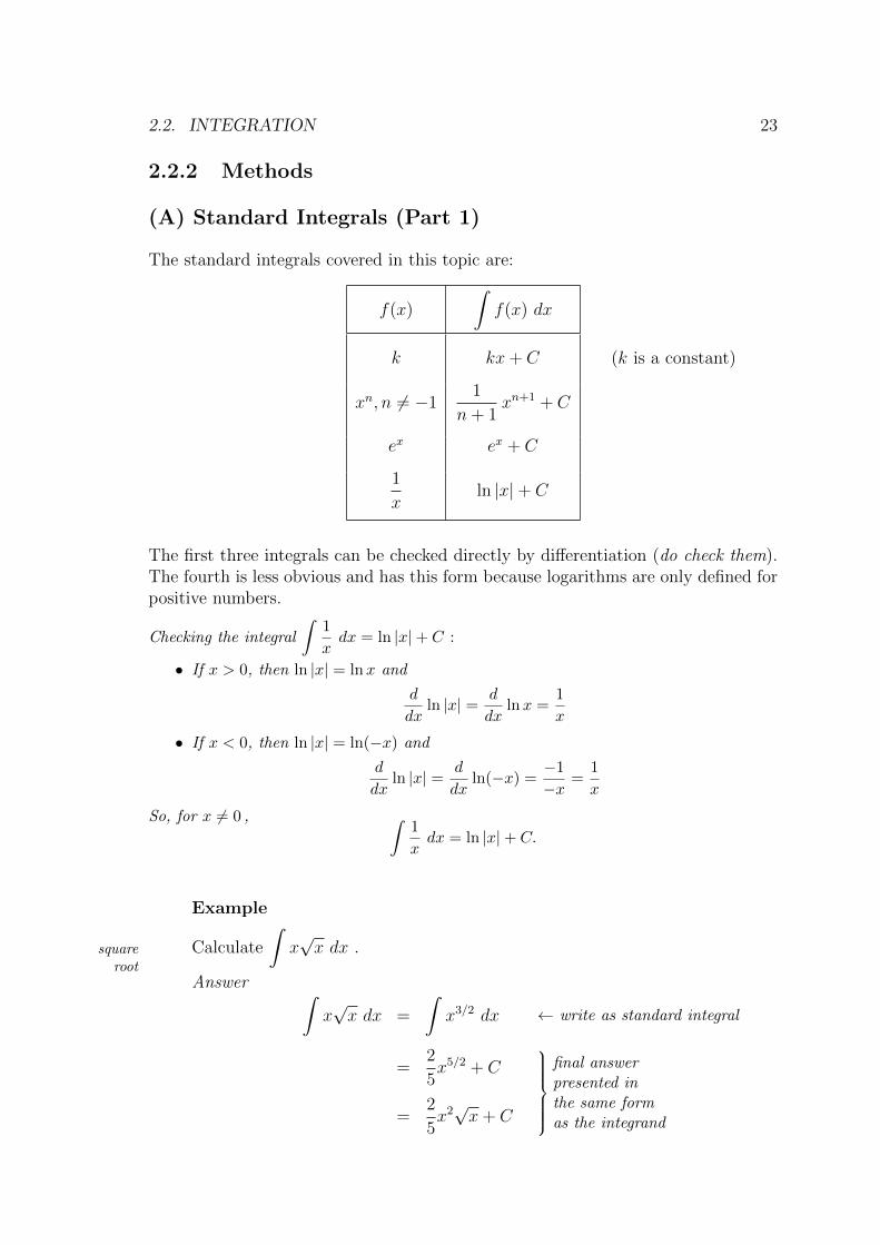
2.2.2 Methods
(A) Standard Integrals (Part 1)
The standard integrals covered in this topic are:
f(x)
∫f(x) dx
k kx+ C
xn, n 6= −11
n+ 1xn+1 + C
ex ex + C
1
xln |x|+ C
(k is a constant)
The first three integrals can be checked directly by differentiation (do check them).The fourth is less obvious and has this form because logarithms are only defined forpositive numbers.
Checking the integral
∫1
xdx = ln |x|+ C :
• If x > 0, then ln |x| = lnx and
d
dxln |x| = d
dxlnx =
1
x
• If x < 0, then ln |x| = ln(−x) and
d
dxln |x| = d
dxln(−x) =
−1
−x=
1
x
So, for x 6= 0 , ∫1
xdx = ln |x|+ C.
← write as standard integral
final answerpresented inthe same formas the integrand
Example
squareroot
Calculate
∫x√x dx .
Answer ∫x√x dx =
∫x3/2 dx
=2
5x5/2 + C
=2
5x2√x+ C
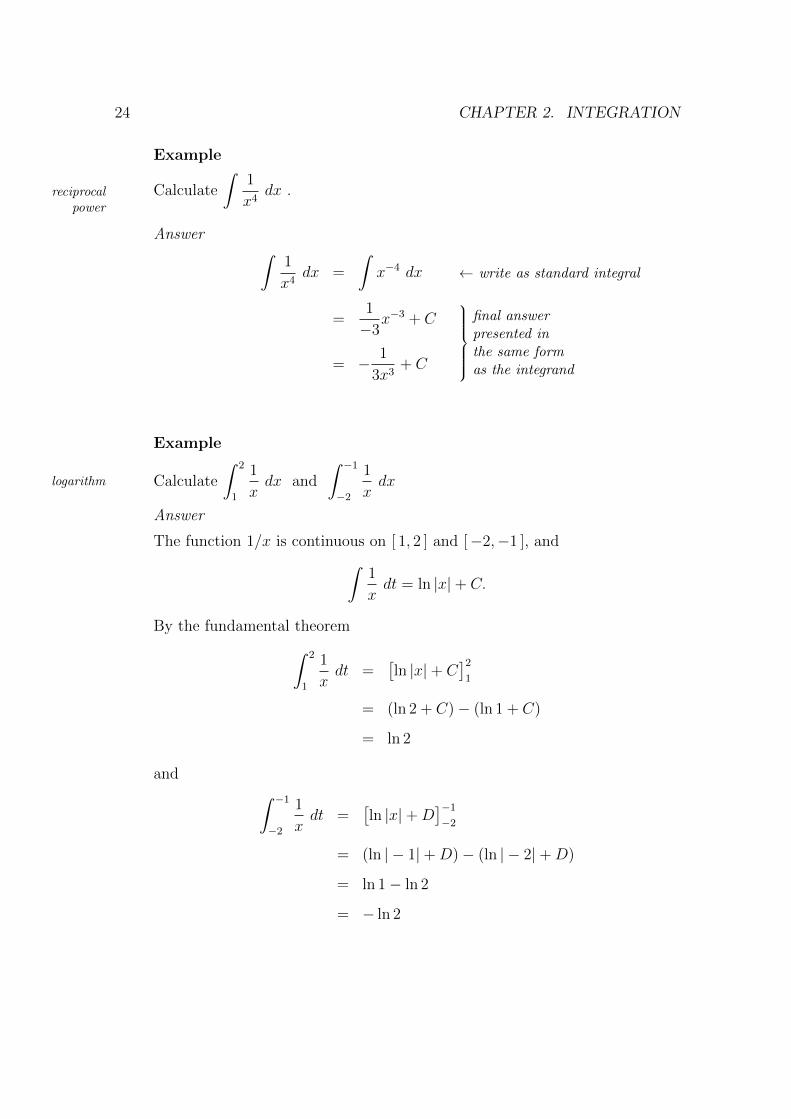
24 CHAPTER 2. INTEGRATION
Example
reciprocalpower
Calculate
∫1
x4dx .
← write as standard integral
final answerpresented inthe same formas the integrand
Answer ∫1
x4dx =
∫x−4 dx
=1
−3x−3 + C
= − 1
3x3+ C
Example
logarithm Calculate
∫ 2
1
1
xdx and
∫ −1−2
1
xdx
Answer
The function 1/x is continuous on [ 1, 2 ] and [−2,−1 ], and∫1
xdt = ln |x|+ C.
By the fundamental theorem∫ 2
1
1
xdt =
[ln |x|+ C
]21
= (ln 2 + C)− (ln 1 + C)
= ln 2
and ∫ −1−2
1
xdt =
[ln |x|+D
]−1−2
= (ln | − 1|+D)− (ln | − 2|+D)
= ln 1− ln 2
= − ln 2

2.2. INTEGRATION 25
Exercise 2.2.2
1. Calculate each of the following integrals.
(a)
∫10 dx (b)
∫−10 dx
(c)
∫ √x dx (d)
∫1√xdx
(e)
∫r2√r dr (f)
∫1
s2√sds
(g)
∫t3 dt (h)
∫1
u3du
2. Use the Fundamental Theorem of Calculus to calculate the following integrals.
(a)
∫ 1
0
ex dx (b)
∫ 0
−1ex dx
(c)
∫ 2
1
1
xdx (d)
∫ −1−2
1
xdx
(e)
∫ T
0
ex dx (f)
∫ S
1
1
xdx, S > 1

26 CHAPTER 2. INTEGRATION
(B) Linear Combinations
Many mathematical functions are constructed from linear combinations of simplerfunctions.vi For example, polynomials are linear combinations of powers.
We may be able to integrate these functions by systematically guessing the integral(or antiderivative) of each term in the linear combination.
This is called integrating term-by-term.
Example
integratingterm-by-term 1. If f(x) = 100x2, then ∫
100x2 dx = 100× 1
3x3 + C
=100
3x3 + C
2. If f(x) = x2 + 2x+ 3, then∫x2 + 2x+ 3 dx =
1
3x3 + 2× 1
2x2 + 3× x+D
=1
3x3 + x2 + 3x+D
3. If f(x) = (x+ 3)(x− 7), then (expanding the brackets first)∫(x+ 3)(x− 7) dx =
∫x2 − 4x− 21 dx
=1
3x3 − 4× 1
2x2 − 21× x+ E
=1
3x3 − 2x2 − 21x+ E
We can summarise this method by the following rules:
Rule 1 (multiples)
The integral of a constant multiple is the multiple of the integral.∫cf(x) dx = c
∫f(x) dx
Rule 2 (sums of terms)
The integral of a sum of terms is the sum of their integrals.∫f(x) + g(x) + . . . dx =
∫f(x) dx +
∫g(x) dx + . . .
viA linear combination of the functions f(x), g(x), h(x) . . . is sum of multiples of the functions,e.g. af(x) + bg(x) + ch(x) + · · · for constants a, b, c . . . For example, x2 − 4x − 21 is a linearcombination of x2, x and 1 with constants 1,−4 and − 21. Its terms are x2,−4x and − 21.

2.2. INTEGRATION 27
Exercise 2.2.2
3. Calculate each of the following integrals.
(a)
∫x2 + 4x+ 8 dx (b)
∫25− 16x3 dx
(c)
∫ √x− 4√
xdx (d)
∫x− 2
xdx
(e)
∫(t+ 1)(t+ 2) dt (f)
∫(2− u)2 du
(g)
∫(v + 1)2
vdv (h)
∫ew − e−w
2dw
4. What is the area of the region enclosed by y = (x+ 1)(x− 3) and the x-axis?

28 CHAPTER 2. INTEGRATION
(C) Standard Integrals (Part 2)
The standard integrals introduced in (A) can be extended to include :
f(x)
∫f(x) dx
(ax+ b)n, n 6= −11
a(n+ 1)(ax+ b)n+1 + C
eax+b1
aeax+b + C
1
ax+ b
1
aln |ax+ b|+ C
for constants a 6= 0 and b.
Each integral in the table can be checked directly by differentiating, using the chainrule. (Do this.)
Example
squareroot
Calculate
∫12√
2x+ 3 dx .
Answer∫12√
2x+ 3 dx = 12
∫(2x+ 3)1/2 dx
= 12× 1
2× 32
(2x+ 3)3/2 + C ← check here vii
= 4(2x+ 3)√
2x+ 3 + C
Example
logarithm Calculate
∫2
3x+ 5dx .
Answer ∫2
3x+ 5dx = 2
∫1
3x+ 5dx
= 2× 1
3ln |3x+ 5|+ C ← check here
=2
3ln |3x+ 5|+ C
viiSee the note on arbitary constants on page 21.
2.2. INTEGRATION 29
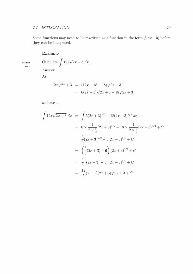
Some functions may need to be rewritten as a function in the form f(ax+ b) beforethey can be integrated.
Example
squareroot
Calculate
∫12x√
2x+ 3 dx .
Answer
As
12x√
2x+ 3 = (12x+ 18− 18)√
2x+ 3
= 6(2x+ 3)√
2x+ 3− 18√
2x+ 3
we have . . .
∫12x√
2x+ 3 dx =
∫6(2x+ 3)3/2 − 18(2x+ 3)1/2 dx
= 6× 1
2× 52
(2x+ 3)5/2 − 18× 1
2× 32
(2x+ 3)3/2 + C
=6
5(2x+ 3)5/2 − 6(2x+ 3)3/2 + C
=
(6
5(2x+ 3)− 6
)(2x+ 3)3/2 + C
=6
5((2x+ 3)− 5) (2x+ 3)3/2 + C
=12
5(x− 1)(2x+ 3)
√2x+ 3 + C

30 CHAPTER 2. INTEGRATION
Exercise 2.2.2
5. Calculate the following integrals.
(a)
∫(3x+ 1)11 dx (b)
∫16(1− 2x)3 dx
(c)
∫2√x+ 5 dx (d)
∫2√p+ 5
dp
(e)
∫12
3q + 7dq (f)
∫ew/2 − e−w/2
2dw
6. Rewrite each integrand in an appropriate form and then calculate the integral.
(a)
∫3x(3x+ 1)11 dx (b)
∫16x(1− 2x)3 dx
(c)
∫2x√x+ 5 dx (d)
∫12q
3q + 7dq

2.2. INTEGRATION 31
(D) Composite Functions
The standard integrals on page 28 were obtained by applying the chain rule to simplefunctions of the form f(ax+ b).
We can extend our integrating skills by making use of the general chain rule forcomposite functions :
The derivative of a composite function is the derivative of the outside functionmultiplied by the derivative of the inside function.
In symbols . . .
The Chain Rule
If f(u) and g(x) are given functions, then
F (x) = f(g(x)) =⇒ F ′(x) = f ′(g(x))g′(x)
. . . giving the indefinite integral :∫f ′(g(x))g′(x) dx = f(g(x)) + C
Integration involves systematic guessing followed by checking using differentiation.The most efficient way to decide if an integral has the form∫
f ′(g(x))g′(x) dx
is to (a) guess which function is the inside function g(x)
(b) confirm the presence of g′(x)
(c) verify that the integrand has the form f ′(g(x))g′(x).
Example
first g(x)
then g′(x)
Calculate
∫x√x2 + 1 dx.
Answer
If g(x) = x2 + 1, then g′(x) = 2x. The integrand has x as a factor rather thang′(x) = 2x, but this shouldn’t be a problem as x = 1
2× 2x.∫
x√x2 + 1 dx =
1
2
∫ √x2 + 1 2x dx
=1
2× 1
3/2(x2 + 1)3/2 + C
=1
3(x2 + 1)
√x2 + 1 + C

32 CHAPTER 2. INTEGRATION
Example
first g(x)
then g′(x)
Calculate
∫x3
x4 + 10dx.
Answer
If g(x) = x4 + 10, then g′(x) = 4x3. The integrand has x3 as a factor ratherthan g′(x) = 4x3, but this isn’t a problem as it is a constant multiple of g′(x).∫
x3
x4 + 10dx =
1
4
∫1
x4 + 104x3 dx
=1
4× ln |x4 + 10|+ C
It was difficult to jump from∫1
x4 + 104x3 to ln |x4 + 10|+ C
in this example. The substitution method below makes this easier.
The substitution or change of variable method makes the integral∫f ′(g(x))g′(x) dx
easier and more straightforward to calculate.
The idea is to simplify the integral by using the new variable u instead of x, whereu = g(x).viii
This is done by replacing
• g(x) by u . . . as u = g(x)
• g′(x) dx by du . . . asdu
dx= g′(x) ix
When this is done∫f ′(g(x))g′(x) dx is transformed to
∫f ′(u) du
with integral f(u) + C = f(g(x)) + C.
Observe the difference when the substitution method is applied to the previous twoexamples (next page).
viiiAny letter can be used to represent a new variable, not just u.
ixWhile it doesn’t make sense to separate the top and bottom parts of the symboldu
dx, the
procedure always leads to a correct outcome. It’s best to think of this as working with the notationin a suggestive way.

2.2. INTEGRATION 33
Example
firstguessg(x)
Calculate
∫x√x2 + 1 dx.
Answer
If g(x) = x2 + 1, then g′(x) = 2x. The integrand has x as a factor rather thang′(x) = 2x, but this shouldn’t be a problem as x = 1
2× 2x.
Put u = x2 + 1, then du = 2x dx, and∫x√x2 + 1 dx =
1
2
∫ √x2 + 1 2x dx
=1
2
∫ √u du
=1
2× 1
3/2u3/2 + C
=1
3u√u+ C
Rewriting the answer in terms of x gives∫x√x2 + 1 dx =
1
3(x2 + 1)
√x2 + 1 + C
Example
first g(x)
then g′(x)
Calculate
∫x3
x4 + 10dx.
Answer
If g(x) = x4 + 10, then g′(x) = 4x3. The integrand has x3 as a factor ratherthan g′(x) = 4x3, but this isn’t a problem as it is a constant multiple of g′(x).
Put u = x4 + 10, then du = 4x3 dx, and∫x3
x4 + 10dx =
1
4
∫1
x4 + 104x3 dx
=1
4
∫1
udu
=1
4ln |u|+ C
Rewriting the answer in terms of x gives∫x3
x4 + 10dx =
1
4ln |x4 + 10|+ C

34 CHAPTER 2. INTEGRATION
Exercise 2.2.2
7. Calculate each of the following integrals.
(a)
∫2x(x2 + 1)3 dx (b)
∫(2x+ 4)(x2 + 4x)4 dx
(c)
∫(x2 + 4)(x3 + 12x+ 1)5 dx (d)
∫2x√x2 + 1 dx
(e)
∫(2t+ 1)
√t2 + t dt (f)
∫u3 + 1√u4 + 4u
du
(g)
∫2v
(v2 + 1)3dv (h)
∫w + 2
(w2 + 4w + 3)5dw
8. Calculate each of the following integrals.
(a)
∫2x ex
2−2 dx (b)
∫x2 ex
3+10 dx
(c)
∫(x+ 1)ex
2+2x−3 dx (d)
∫e1/x
x2dx
(e)
∫et(et + 10)5 dt (f)
∫e2u√e2u + 1 du
(g)
∫10ev
(ev + 1)3dv (h)
∫e2w + 2ew
(e2w + 4ew + 3)5dw
9. Calculate each of the following integrals.
(a)
∫3x2
x3 + 1dx (b)
∫2x+ 4
x2 + 4xdx
(c)
∫x2 + 4
x3 + 12x+ 1dx (d)
∫ex
ex + 1dx
(e)
∫e2t + 3et
e2t + 6et + 10dt (f)
∫eu − e−u
eu + e−udu

2.2. INTEGRATION 35
(E) Numerical Methods (optional)
There are many antiderivatives that can not be found explicitly, for example∫ex
2
dx.
In these cases we use numerical methods to estimate their definite integrals. Themethod of using upper and lower methods to estimate an integral is one such method,but there are other methods that provide closer closer approximations and are easierto program.
See
http://en.wikipedia.org/wiki/Numerical integration
http://en.wikibooks.org/wiki/Numerical Methods/Numerical Integration
and
http://people.hofstra.edu/Stefan Waner/realworld/integral/numint.html
http://people.hofstra.edu/Stefan waner/realworld/integral/integral.html
[All pages accessed 18/3/08]

36 CHAPTER 2. INTEGRATION
2.2.3 Selected Applications
Integration has widespread applications in science and engineering including :
• calculation of areas
• calculation of volumes
• calculation of centres of mass of solids
• calculation of the work done by a force
• problems concerned with rate of change
• problems in economics
• statistical problems
This topic only considers problems associated with areas and change in quantitiesover time.
(I) Calculation of the area between two curves
We have seen in section 1.3 that if f(x) is a continuous function for a ≤ x ≤ b, then∫ b
a
f(x) dx
is equal to the the difference between
• the sum of the areas under f(x) and above the x-axis
• the sum of the areas above f(x) and below the x-axis
for a ≤ x ≤ b.
Let f(x) and g(x) be positive continuous functions for a ≤ x ≤ b. Suppose also thatf(x) ≥ g(x) on [ a, b ]. This is shown in the diagram below.
What is the area of the shaded region between f(x) and g(x) that is bounded by thelines x = a and x = b?
-�x
y = f(x)
y = g(x)
a b

2.2. INTEGRATION 37
The area remains the same if each curve is translated vertically by the same distancek, with k taken so that both curves are above the x-axis.
-�x
y = f(x) + k
y = g(x) + k
a b
You can now be seen that the area of the shaded region is the difference betweenthe areas below:
-�x
y = f(x) + k
y = g(x) + k
a b
Area1 =
∫ b
a
(f(x) + k) dx
-�x
y = f(x) + k
y = g(x) + k
a b
Area2 =
∫ b
a
(g(x) + k) dx

38 CHAPTER 2. INTEGRATION
. . . and that the difference in areas is
A =
∫ b
a
(f(x) + k)− (g(x) + k) dx =
∫ b
a
f(x)− g(x) dx
In general,
If f(x) and g(x) are continuous functions for a ≤ x ≤ b, then∫ b
a
f(x)− g(x) dx
is equal to the the difference between
(a) the area under f(x) and above g(x) when f(x) ≥ g(x)
(b) the area under g(x) and above f(x) when g(x) ≥ f(x)
for a ≤ x ≤ b.
Example
areabetween
curves
What is the area of the region enclosed by the parabola y = x2 and the liney = x?
-�x
6
?
y
0 1
Answer
The parabola and line intersect when
x2 = x
x2 − x = 0
x(x− 1) = 0
x = 0 & 1

2.2. INTEGRATION 39
The enclosed area is ∫ 1
0
x− x2 dx =
[x2
2− x3
3+ C
]10
=
[1
2− 1
3
]− 0
=1
6

40 CHAPTER 2. INTEGRATION
Exercise 2.2.3
1. Calculate the area between the curves below over the given interval
(a) f(x) = x2 − 4 and g(x) = −x2 + 9 −1 ≤ x ≤ 1
(b) f(x) = x2 and g(x) = x3 0 ≤ x ≤ 1
(c) f(x) = 2x and g(x) = −x2 + 3 −3 ≤ x ≤ 1
(e) f(x) = ex and g(x) = x 0 ≤ x ≤ 3
2. Calculate the area enclosed by the curves below
(a) f(x) = x and g(x) = x2
(b) f(x) =√x and g(x) = x2
(c) f(x) = x4 and g(x) = 3x2
(d) f(x) = x4 and g(x) = −2x2 + 3
3. The cable used to construct a new arts centre will have the cross-section shownbelow.
-�x
6
?
yy = (x− 0.2)2
↙
(a) Express the cross-sectional area as an integral.
(b) Calculate the area.
(c) If 300 m of cable are requied, calculate the volume of the cable.
4. Consider the graphs of the form y = xn for positive integers n.
(a) At what points do these graphs intersect?
(b) Does the area between the graphs and the x-axis, from x = 0 to x = 1increase or decrease as n increases?
(c) What happens if the interval in (b) was changed to [ 0, 2 ]?
(d) What happens if n is allowed to be a negative integer?

2.2. INTEGRATION 41
(II) Change in Quantities
We discovered in section 1.3 that if the rate of change of a quantity is known and ispositive, then the net change in the quantity is equal to the area under the graph ofthe rate of change and above the horizontal axis.
The Fundamental Theorem in section 2.1 extends this discovery:
Net Change
If the rate of change f(x) with respect to x is known for a quantity F (x),then the net change in the quantity from x = a to x = b is
F (b)− F (a) =
∫ b
a
f(x) dx
Example
totalchange
The maintenance costs M(x) for a building increase with age x years. Recordsfor a certain building show that the rate of increase in costs is approximately
dM
dx= 60x2 + 400 dollars/year.
What is the total maintenance cost for
(a) the first 5 years?
(b) the first t years?
Answer
(a) The total cost for the first 5 years is∫ 5
0
60x2 + 400 dx =[20x3 + 400x+ C
]50
=[20× 53 + 400× 5
]− 0
= $ 4500
(b) The total cost for the first t years is∫ t
0
60x2 + 400 dx =[20x3 + 400x+D
]t0
= 20t3 + 400t dollars

42 CHAPTER 2. INTEGRATION
Example
definiteintegral
vs
indefiniteintegral
The marginal cost x of manufacturing x radios per week is
dC
dx= 25− 0.1x dollars/radio
when 0 ≤ x ≤ 200. The fixed costs per week before production begins are$ 1000.xi
What is the total cost of producing 100 radios per week?
Answer (definite integral)
As
Total Cost = Fixed Costs + Cost of Production
we have
Total cost (100 radios) = 1000 +
∫ 100
0
25− 0.1x dx
= 1000 +[25x− 0.05x2 + C
]1000
= 1000 +[25× 100− 0.05× 1002
]− 0
= $ 3000
Answer (indefinite integral)
As the marginal cost isdC
dx= 25− 0.1x, the cost of production is
C(x) =
∫25− 0.1x dx
= 25x− 0.05x2 + C
for some constant C and, as C(0) = 0⇒ C = 0,
= 25x− 0.05x2
So
Total cost (100 radios) = 1000 + C(100)
= 1000 + (25× 100− 0.05× 1002)
= $ 3000
xThe marginal cost of production is the rate of change of cost of production relative to output.xiThe fixed costs are necessary costs that are independent of the number of radios produced.
They might include lease, wages, insurance, etc.

2.2. INTEGRATION 43
When an object travels along a straight line, its displacement s(t) is its positionfrom the origin. A positive displacement corresponds to a position on the right ofthe origin, and a negative displacement corresponds to a position on the left of theorigin. If the object moves 1m away from the origin then returns to the origin itsdisplacement will be zero even though the distance travelled is 2m.
Velocity v(t) is the rate of change of displacement, s′(t). An object travelling ina positive direction has a positive velocity. When it returns towards the origin itsvelocity is negative.
Example
velocity
displacementdistance
A object P moves in a straight line with velocity
v(t) =ds
dt= 2− 2t m/s.
for t ≥ 0 seconds. What is
(a) its change in displacement between t = 0 and t = 1?
(b) the distance it travelled between t = 0 and t = 1?
(c) its change in displacement between t = 0 and t = 2?
(d) the distance it travelled between t = 0 and t = 2?
Answer
(a) The change in displacement between t = 0 and t = 1 is
s(1)− s(0) =
∫ 1
0
2− 2t dt
=[2t− t2 + C
]10
= 1 m
(b) As v(t) ≥ 0 for 0 ≤ t ≤ 1,
distance travelled =
∫ 1
0
2− 2t dt
=[2t− t2 + C
]10
= 1 m
(c) The change in displacement between t = 0 and t = 2 is
s(2)− s(0) =
∫ 2
0
2− 2t dt
=[2t− t2 + C
]20
= 0 m

44 CHAPTER 2. INTEGRATION
(d) As v(t) ≥ 0 for 0 ≤ t ≤ 1, and v(t) ≤ 0 for 1 ≤ t ≤ 2
distance travelled =
∫ 1
0
2− 2t dt−∫ 2
1
2− 2t dt
=[2t− t2 + C
]10−[2t− t2 +D
]21
= 1− (−1)
= 2 m

2.2. INTEGRATION 45
Exercise 2.2.3
5. The marginal cost of manufacturing and storing x cardboard cartons per weekis
C ′(x) = 3.2 + 0.0004x dollars per item,
and the fixed costs are $500 per week.
What is the total cost of manufacturing and storing 1000 cartons per week?
6. A new suburb is estimated to grow at the rate of
dP
dt= 1500 + 300
√t
people per year. If the current population is 1000, estimate
(a) the population in 25 years
(b) the population P (t) after t years
7. The area A(t) covered by an ulcer changes at a rate
dA
dt= − 4
(t+ 1)2cm2/day
as it heals, where t is in days. If the area is initially A(0) = 4 cm2, what is
(a) the area of the wound in 10 days
(b) the area A(t) sfter t days
8. A object P moves in a straight line with velocity
v(t) =ds
dt= 2− t2 m/s.
for t ≥ 0 seconds. What is the
(a) change in displacement between t = 0 and t = 1?
(b) distance it travelled between t = 0 and t = 1?
(c) change in displacement between t = 0 and t = 2?
(d) distance it travelled between t = 0 and t = 2?
9. A oil tanker hit a reef and is producing a circular oil slick that is expandingat an approximate rate of
dr
dt=
20√t+ 1
where r metres is the radius of the slick after t minutes. If r(0) = 20, estimate
(a) the radius of the slick after 30 minutes
(b) the radius of the slick after t minutes

46 CHAPTER 2. INTEGRATION
(c) the rate at which the area of the slick is changing
10. A circular plastic tube, with internal diameter 4 cm and external diameter 4.5cm, carries water at a constant temperature of 70◦C. The temperature insidethe tube drops off at a rate of
dT
dx= −5
x
where x is the distance from the centre of the tube and 4 ≤ x ≤ 4.5. What isthe temperature on the outside of the tube?

Appendix A
Summation Notation
Summation notationi is used in situations where we need to write down the sum ofmany numbers or terms. We could write the sum of the squares of the numbers from1 to 100 as
12 + 22 + 32 + . . . + 1002 ,
leaving it to the reader to guess the pattern of numbers, but summation notationcan be used to express this sum concisely and without ambiguity as
100∑i=1
i2 .
If f(i) represents an expression involving i, then
n∑i=1
f(i)
has the following meaning :
n∑i=1
f(i) = f(1) + f(2) + f(3) + . . . + f(n) .
This notation has a number of parts :
summation sign -
end
?
index�
startJJ]
general term�
n∑i=1
f(i)
iSometimes sigma notation because the Greek letter sigma Σ is used.
47

48 APPENDIX A. SUMMATION NOTATION
• The summation sign Σ
Σ is the Greek upper case letter corresponding to “S”. It tells us to add theterms in a sum, where the general term is given to the right of the summationsign.
• The index variable i
This variable is used to number or label each term in the sum. The index isoften represented by i. Other common possibilities include j and k.
• The start
The ”i =” part beneath the summation sign tells shows which index numberto begin with. It is usually either zero or one but it can be anything. Youalways increase the index by one at each successive step in the sum.
• The end
The number on top of the summation sign is the final index number.
Example
sum ofindexed
terms
(a)50∑i=0
i2 = 02 + 12 + 22 + . . . + 502
(b)50∑j=1
j2 = 12 + 22 + 32 + . . . + 502
(c)15∑k=3
1
k=
1
3+
1
4+
1
5+ . . . +
1
15
(d)8∑t=0
(−1)i2
1 + i=
2
1 + 0− 2
1 + 1+
2
1 + 2− . . . +
2
1 + 8
(e)n∑t=1
3√t = 3
√1 + 3
√2 + 3
√3 + . . . + 3
√n
Appendix B
Justification for the FundamentalTheorem
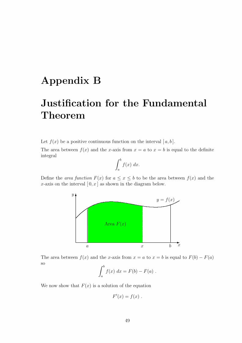
Let f(x) be a positive continuous function on the interval [ a, b ].
The area between f(x) and the x-axis from x = a to x = b is equal to the definiteintegral ∫ b
a
f(x) dx.
Define the area function F (x) for a ≤ x ≤ b to be the area between f(x) and thex-axis on the interval [ 0, x ] as shown in the diagram below.
y = f(x)
Area F (x)
6y
-xa x b
The area between f(x) and the x-axis from x = a to x = b is equal to F (b)− F (a)so ∫ b
a
f(x) dx = F (b)− F (a) .
We now show that F (x) is a solution of the equation
F ′(x) = f(x) .
49

50 APPENDIX B. JUSTIFICATION FOR THE FUNDAMENTAL THEOREM
The area between f(x) and the x-axis on the interval from 0 to x + h is equal toF (x+ h).
It can be seen from the diagram below that when h is very small this area is closelyapproximated by adding
• the area between f(x) and the x-axis from 0 to x
• the area of the rectangle with height f(x) and base the interval [x, x+ h ].
y = f(x)
Area F (x)
6y
-xa x ↑
x + h
b
In other wordsF (x+ h) ≈ F (x) + hf(x)
andF (x+ h)− F (x)
h≈ f(x) .
We know that as h becomes very small,
F (x+ h)− F (x)
h→ F ′(x)
which impliesF ′(x) = f(x) .
So ∫ b
a
f(x) dx = F (b)− F (a) ,
where F (x) is a solution of the equation
F ′(x) = f(x) .
The final step in the justification is to show that this is true for any function thatsatisfies F ′(x) = f(x) . . .

51
If G(x) is another function with G′(x) = f(x), then
d
dx(G(x)− F (x)) = G′(x)− F ′(x) = 0 .
This implies that G(x)− F (x) = k for some constant k.
AsG(b)−G(a) = (F (b) + k)− (F (a) + k) = F (b)− F (a)
you can see that ∫ b
a
f(x) dx = F (b)− F (a) = G(b)−G(a) ,
. . . so it doesn’t matter which solution of F ′(x) = f(x) is chosen.
Appendix C
Answers
Exercise 1.1
1(a) Horizontal line with vertical intercept (0, 1000).
1(b) From graph, V (t) = 10t.
1(c) Line with gradient 10 and vertical intercept (0, 100).
1(d) Rate of change of volume per minute.
2(a) Straight line with intercepts (60, 0) and (0, 30).
2(b) 900 m.
2(c) 30t− 0.25t2
3(iii) Upper estimate = 0.76, Lower estimate = 0.56
Exercise 1.2
1(a) Upper estimate = 0.875 , Lower estimate = 0.375.
1(b) Ten equal intervals of width 0.1.
2(a) Upper estimate = 1.75 , Lower estimate = 0.75.
Exercise 1.3
1(i) 2 1(ii) −2 1(iii) 1
2. The graph of 1 + sin(x) is obtained by translating the graph of sin(x) verticallyby one unit. The area is 2 + 1× π = 2 + π
52

53
Exercise 1.4
1(i) 20 1(ii)11
61(iii) −7
62(b) c− a− b
Exercise 2.1
2. 21
Exercise 2.2.1
1(a)1
4x4 + C 1(b) 2x5 +D 1(c)
7
3x3 + E
1(d)1
3x3 + x2 + x+ F 1(e) 8x1/2 +G 1(f) 20e5t +H
2(a)1
4x4 + C 2(b)
3
8x8 +D 2(c)
1
3x3 + x2 + 3x+ E
2(d) −2r−2 + F 2(e)2
3t3/2 +G 2(f) 2w1/2 +H
3(a)1
33(b) 126 3(c)
14
3
3(d) 4 3(e)224
33(f) 16(
√2− 1)
Exercise 2.2.2
1(a) 10x+ C 1(b) −10x+D 1(c)2
3x√x+ E
1(d) 2√x+ F 1(e)
2
7r3√r +G 1(f) − 2
3s√s
+H
1(g)1
4t4 + I 1(e) −1
2u−2 + J
2(a) e− 1 2(b) 1− e−1 2(c) ln 2
2(d) − ln 2 2(e) eT − 1 2(f) lnS
3(a)1
3x3 + 2x2 + 8x+ C 3(b) 25x− 4x4 +D
3(c)2
3x√x− 8
√x+ E 3(d)
1
2x2 − 2 ln |x|+ F
3(e)1
3t3 +
3
2t2 + 2t+G 3(f) 4u− 2u2 +
1
3u3 +H
3(g)1
2v2 + 2v + ln v + I 3(h)
ew + e−w
2+ J

54 APPENDIX C. ANSWERS
4.32
3
5(a)1
36(3x+ 1)12 + C 5(b) −2(1− 2x)4+D
5(c)4
3(x+ 5)
√x+ 5 + E 5(d) 4
√p+ 2 + F
5(e) 4 ln |3q + 7|+G 5(f) ew/2 + e−w/2 +H
6(a)
∫(3x+ 1)12 − (3x+ 1)11 dx =
1
39(3x+ 1)13 − 1
36(3x+ 1)12 + C
6(b)
∫−8(1− 2x)4 + 8(1− 2x)3 dx =
4
5(1− 2x)5 − (1− 2x)4 +D
6(c)
∫2(x+ 5)3/2 − 10(x+ 5)1/2 dx⇒ 4
5(x+ 5)2
√x+ 5− 20
3(x+ 5)
√x+ 5 + E
6(d)
∫4− 28
3q + 7dq = 4q − 28
3ln |3q + 7|+ F
7(a)1
4(x2 + 1)4 + C 7(b)
1
5(x2 + 4x)5 +D
7(c)1
18(x3 + 12x+ 1)6 + E 7(d)
2
3(x2 + 1)
√x2 + 1 + F
7(e)2
3(t2 + t)
√t2 + t+G 7(f)
1
2
√u4 + 4u+H
7(g) − 1
2(v2 + 1)2+ I 7(h) − 1
8(w2 + 4w + 3)4+ J
8(a) ex2−2 + C 8(b)
1
3ex
3+10 +D
8(c)1
2ex
2+2x−3 + E 8(d) −e1/x + F
8(e)1
6(et + 10)6 +G 8(f)
1
3(e2u + 1)3/2 +H
8(g) − 5
(ev + 1)2+ I 8(h) − 1
8(e2w + 4ew + 3)4+ J
9(a) ln |x3 + 1|+ C 9(b) ln |x2 + 4x|+D
9(c)1
3ln |x3 + 12x+ 1|+ E 9(d) ln |ex + 1|+ F
9(e)1
2ln |e2t + 6et + 10|+G 9(f) ln |eu + e−u|+H

55
Exercise 2.2.3
1(a)76
31(b)
1
121(c)
32
31(d) e3 − 11
2
2(a)1
62(b)
1
32(c)
12√
3
52(d)
64
15
3(a) 4
∫ 0.2
0
(x− 0.2)2 dx 3(b)4
375m2 3(c) 3.2 m3
4(a) They all intersect at (0, 0) and (1, 0).
4(b) The area between y = xn and x-axis from x = 0 to x = 1 is
1
n+ 1,
which decreases as n increases.
4(c) The area would then be2n+1
n+ 1,
which increases as n increases. You can check this last statement by consider-ing
2n+1
n+ 1− 2n
n= 2n
(2
n+ 1− 1
n
)= 2n
(n− 1
n(n+ 1)
)≥ 0
4(d) The area is infinite when n ≤ −1. You can check this by calculating the areafrom x = h to x = 1 for h > 0.
For example, for n = −1 it is∫ 1
h
x−1 dx = [ln |x|]1h = − lnh,
which becomes infinite as h→ 0.
Note. We couldn’t calculate the integral directly for the interval [ 0, 1 ] as x−1
is not defined for x = 0.
Check out what happens with x =1
2!
5. Total Cost = 500 +
∫ 1000
0
3.2 + 0.0004x dx = $3900
6(a) P (25) = 1000 +
∫ 25
0
1500 + 300√t dt = 63, 500
6(b) P (t) = 1000 +
∫ t
0
1500 + 300√t dt = 1000 + 1500t+ 200t
√t

56 APPENDIX C. ANSWERS
7(a) A(10) = 4 +
∫ 10
0
− 4
(t+ 1)2dt =
4
11cm2
7(b) A(t) = 4 +
∫ t
0
− 4
(t+ 1)2dt =
4
t+ 1cm2
8(a) s(1)− s(0) =
∫ 1
0
2− t2 dt =5
3cm
8(b) distance travelled =
∫ 1
0
2− t2 dt =5
3cm
8(c) s(1)− s(0) =
∫ 2
0
2− t2 dt =4
3cm
8(d) distance travelled =
∫ √20
2− t2 dt−∫ 2
√2
2− t2 dt =8√
2− 4
3cm
9(a) r(30) = r(0) +
∫ 30
0
20√t+ 1
dt = 10 + 10√
31 cm
9(b) r(t) = r(0) +
∫ t
0
20√t+ 1
dt = 10 + 10√t+ 1 m
9(c) A(t) = π(10 + 10√t+ 1)2 = 100π(2 + 2
√t+ 1 + t) m2
⇒ A′(t) = 100π
(1 +
1√t+ 1
)m2/min
10. T (4.5) = T (4) +
∫ 4.5
4
−5
xdx = 70 + 5 ln(4/4.5) ◦C