module v - cectl.ac.in

1

Lecture Note – Mr. Sarath V Sankaran, JCET

MODULE – V

Digital Data Communication Techniques - Asynchronous transmission, Synchronous transmission-

Detecting and Correcting Errors-Types of Errors-Error Detection: Parity check, Cyclic Redundancy

Check (CRC) - Error Control Error Correction: Forward Error Correction and Hamming Distance.

1. Digital Data Communication Types

1.1 Parallel and serial mode

Digital data transmission can occur in two basic modes:

1) Parallel Communication:

This transmission involves grouping several bits, say n, together and sending all the n bits at

a time.

Figure hows how parallel transmission occurs for n = 8. This can be accomplishes with the

help of eight wires bundled together in the form of a cable with a connector at each end.

Additional wires, such as request (req) and acknowledgement (ack) are required for

asynchronous transmission.

Primary advantage of parallel transmission is higher speed, which is achieved at the expense

of higher cost of cabling.

Parallel transmission is feasible for short distances.

2) Serial Communication:

This transmission involves sending one data bit at a time.

Figure shows how serial transmission occurs; it uses a pair of wire for communication of data

in bit-serial form.

2


Since communication within devices is parallel, it needs parallel-to-serial and serial-to-

parallel conversion at both ends.

However, it is slower than parallel mode of communication, serial mode of communication is

widely used because of the following advantages:

o Reduced Cost of Cabling: Lesser number of wires is required as compared to parallel

connection.

o Reduced Cross Talk: Lesser number of wires result in reduced cross talk.

o Inherent Device Characteristics: Many devices are inherently serial in nature.

o Portable device like PDAs, etc., use serial communication to reduce the size of the

connector.

Difference between Serial and Parallel Communication

Serial Communication Parallel Communication

The data is transmitted by sending one bit per each clock pulse.

The stream of bits is divided into groups and one group is sent per each clock pulse.

It is a slower mode of transmission, as only one bit can be transmitted at a time.

It is a faster mode of transmission, as several bits can be transmitted at a time.

It requires only one communication channel between communicating devices; thus, it is a cheaper mode of transmission

To send n bits at a time, it requires n communication channel between communicating devices. As a result, cost is increased by a factor of n as compared to serial transmission.

As communication within devices is parallel, both sender and receiver require convener at the interface between the device and the communication channel.

No such converters are required.

1.2 Asynchronous and synchronous transmission

Synchronous transmissions are synchronized by an external clock, while asynchronous

transmissions are synchronized by special signals along the transmission medium.

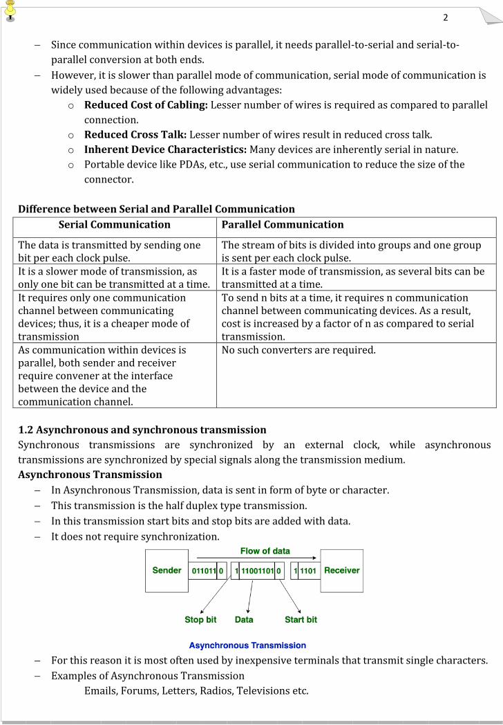
Asynchronous Transmission

In Asynchronous Transmission, data is sent in form of byte or character.

This transmission is the half duplex type transmission.

In this transmission start bits and stop bits are added with data.

It does not require synchronization.

For this reason it is most often used by inexpensive terminals that transmit single characters.

Examples of Asynchronous Transmission

Emails, Forums, Letters, Radios, Televisions etc.

3


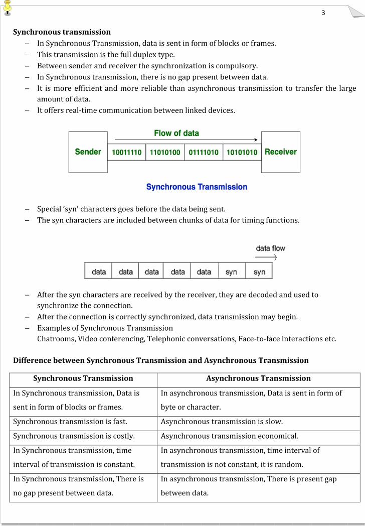
Synchronous transmission

In Synchronous Transmission, data is sent in form of blocks or frames.

This transmission is the full duplex type.

Between sender and receiver the synchronization is compulsory.

In Synchronous transmission, there is no gap present between data.

It is more efficient and more reliable than asynchronous transmission to transfer the large

amount of data.

It offers real-time communication between linked devices.

Special ’syn’ characters goes before the data being sent.

The syn characters are included between chunks of data for timing functions.

After the syn characters are received by the receiver, they are decoded and used to

synchronize the connection.

After the connection is correctly synchronized, data transmission may begin.

Examples of Synchronous Transmission

Chatrooms, Video conferencing, Telephonic conversations, Face-to-face interactions etc.

Difference between Synchronous Transmission and Asynchronous Transmission

Synchronous Transmission Asynchronous Transmission

In Synchronous transmission, Data is

sent in form of blocks or frames.

In asynchronous transmission, Data is sent in form of

byte or character.

Synchronous transmission is fast. Asynchronous transmission is slow.

Synchronous transmission is costly. Asynchronous transmission economical.

In Synchronous transmission, time

interval of transmission is constant.

In asynchronous transmission, time interval of

transmission is not constant, it is random.

In Synchronous transmission, There is

no gap present between data.

In asynchronous transmission, There is present gap

between data.

4


2. Error Control

If there is a change in one data stream (a bit) which is transferred and received, then error

occurs. For example, if 1 is transferred and 0 is received or reverse of it.

2.1 Types of Errors

There are two types of errors are occurred in digital transmission systems:

1) Single-bit Errors: If there is a change in a single bit then the error is known as single bit

error i.e., 1 is changed to 0 or vice versa

2) Burst/Multiple-bit Errors Whenever two or more bits are changed in a given stream: then

this error is known as burst errors.

2.2 Error Control

Data can be corrupted during transmission. For reliable communication, errors must be

detected and corrected.

Error control provides error detection and correction.

There are two basic strategies for dealing with errors.

1) To include only enough redundancy to allow the receiver to confirm that an error

occurred, but not aware of which error and therefore request it for re-transmission.

2) Second method is to include enough unwanted data along with each block of data sent to

enable to receiver to extract what the transmitted character must have been.

2.2.1 Error Detection

Error detection means to decide whether the received data is correct or not without having a

copy of the original message.

Error detection uses the concept of redundancy, which means adding extra bits for detecting

error at the destination.

Error detection often uses error detecting codes. Error detecting code is to include only

enough redundancy to allow the receiver to deduce that an error occurred, but not which

error, and have it request a retransmission.

There are following four error detection methods:

1) VRC (Vertical Redundancy Check)

2) LRC (Longitudinal Redundancy Check)

3) CRC (Cyclic Redundancy Check)

4) Checksum Error Detection

5


Parity Check/Vertical Redundancy Checking (VRC)

It is also known as parity check

It is least expensive mechanism for error detection

In this technique, the redundant bit called parity bit is appended to every data unit so that the

total number of 1s in the unit becomes even (including parity bit)

Example :

1110110 1101111 1110010

- After adding the parity bit

11101101 11011110 11100100

When parity checking is used, an error that changes one bit in a character can be detected

because the parity bit will be incorrect.

VRC can detect all single – bit errors

It can detect burst errors if the total number of errors in each data unit is odd.

VRC cannot detect errors where the total number of bits changed is even. If two 0 bits are

changed to Is, the VRC will not detect the error because the number of 1 bits will still be an

even number. So an odd number of bit errors can be detected, but an even number cannot.

Therefore, more sophisticated checking techniques are employed in most data transmission

systems.

Longitudinal Redundancy Check (LRC)

In this method, a block of bits is organized in table(rows and columns) calculate the parity bit

for each column and the set of this parity bit is also sending with original data.

From the block of parity we can check the redundancy.

6


Suppose the following block is sent :

10101001 00111001 11011101 11100111 10101010

(LRC)

However, it is bit by burst of length eight and some bits are corrupted:

10100011 10001001 11011101 11100111 10101010

(LRC)

When the receiver checks the LRC, some of the bits are not follow even parity rule and whole block

is discarded.

10100011 10001001 11011101 11100111 10101010

Advantage:

LRC of n bits can easily detect burst error of n bits.

Disadvantage:

If two bits in one data units are damaged and two bits in exactly same position in another

data unit are also damaged, the LRC checker will not detect the error.

Cyclic Redundancy Check (CRC)

The sending device performs binary division and CRC remainder is appended to original data

before transmission and sends to the receiving device.

At its destination, the incoming data unit is divided by the same number. If at this step there

is no remainder, the data unit assumes to be correct and is accepted, otherwise it indicates

that data unit has been damaged in transmission and therefore must be rejected.

At sender side,

1. A string of n 0’s (one less than the number of bits in divisor) is appended to the data unit to

be transmitted.

2. Binary division is performed of the resultant string with the CRC generator.

3. After division, the remainder so obtained is called as CRC.

4. The string of 0’s appended to the data unit earlier is replaced by the CRC remainder.

5. The newly formed code word (Original data + CRC) is transmitted to the receiver.

7


At receiver side,

1. The transmitted code word is received.

2. The received code word is divided with the same CRC generator.

3. On division, the remainder so obtained is checked.

4. If the remainder is zero, Receiver assumes that no error occurred in the data during the

transmission. Receiver accepts the data.

5. If the remainder is non-zero, Receiver assumes that some error occurred in the data during

the transmission. Receiver rejects the data and asks the sender for retransmission.

Sender

Receiver

8


Checksum Error Detection

Suppose our data is a list of five 4-bit numbers that we want to send to a destination. In

addition to sending these numbers, we send the sum of the numbers.

For example, if the set of numbers is (7, 11, 12, 0, 6), we send (7, 11, 12, 0, 6, 36), where 36 is

the sum of the original numbers. The receiver adds the five numbers and compares the result

with the sum. If the two are the same, the receiver assumes no error, accepts the five

numbers, and discards the sum. Otherwise, there is an error somewhere and the data are not

accepted.

In checksum error detection scheme, the data is divided into k segments each of m bits.

In the sender’s end the segments are added using 1’s complement arithmetic to get the sum.

The sum is complemented to get the checksum.

The checksum segment is sent along with the data segments.

At the receiver’s end, all received segments are added using 1’s complement arithmetic to get

the sum. The sum is complemented.

If the result is zero, the received data is accepted; otherwise discarded.

2.2.2 Error Correction

Error correction is much more difficult than error detection.

The most commonly used error correction methods are:

1) Retransmission/Reverse Error Correction: In error correction by retransmission,

when an error is detected, the receiver can have the sender retransmit the entire data

unit. Reverse error correction methods are stop and wait, go-back-N or selective

retransmission.

2) Forward Error Correction: In forward error correction method, a receiver can use an

error-correcting code, which automatically corrects certain errors. Block parity, Hamming

code, interleaved code and convolutional code are some of the forward error correction

methods.

9


Hamming Code

It is a technique developed by R.W.Hamming in the late 1940s.

Hamming code can be applied to data units of any length and uses the relationship between

data and redundancy bits.

Redundant bits are extra binary bits that are generated and added to the information-

carrying bits of data transfer to ensure that no bits were lost during the data transfer.

The number of redundant bits can be calculated using the following formula:

2^r ≥ m + r + 1

where, r = redundant bit, m = data bit

Suppose the number of data bits is 7, then the number of redundant bits can be calculated

using: = 2^4 ≥ 7 + 4 + 1 Thus, the number of redundant bits= 4

These redundancy bits are placed at the positions which correspond to the power of 2.

As in the above example:

The number of data bits = 7

The number of redundant bits = 4

The total number of bits = 11

The redundant bits are placed at positions corresponding to power of 1, 2, 4, and 8

Suppose the data to be transmitted is 1011001, the bits will be placed as follows:

Determining the Parity bits –

1. R1 bit is calculated using parity check at all the bits positions whose binary representation

includes a 1 in the least significant position.

R1: bits 1, 3, 5, 7, 9, 11


includes a 1 in the second position from the least significant bit.

R2: bits 2,3,6,7,10,11

10



includes a 1 in the third position from the least significant bit.

R4: bits 4, 5, 6, 7


includes a 1 in the fourth position from the least significant bit.

R8: bit 8,9,10,11

Thus, the data transferred is:

Error detection and correction –

Suppose in the above example the 6th bit is changed from 0 to 1 during data transmission, then it

gives new parity values in the binary number:

The bits give the binary number as 0110 whose decimal representation is 6. Thus, the bit 6

contains an error. To correct the error the 6th bit is changed from 1 to 0.

11


Hamming Distance

Hamming distance is a metric for comparing two binary data strings. While comparing two

binary strings of equal length, Hamming distance is the number of bit positions in which the

two bits are different.

The Hamming distance between two strings, a and b is denoted as d(a,b).

It is used for error detection or error correction when data is transmitted over computer

networks. It is also using in coding theory for comparing equal length data words.

Calculation of Hamming Distance

In order to calculate the Hamming distance between two strings, and , we perform their XOR

operation, (a⊕ b), and then count the total number of 1s in the resultant string.

Example 1:

Suppose there are two strings 1101 1001 and 1001 1101.

11011001 ⊕ 10011101 = 01000100. Since, this contains two 1s, the Hamming distance,

d(11011001, 10011101) = 2.

Minimum Hamming Distance

In a set of strings of equal lengths, the minimum Hamming distance is the smallest Hamming

distance between all possible pairs of strings in that set.

Example 2:

Suppose there are four strings 010, 011, 101 and 111.

010 ⊕ 011 = 001, d(010, 011) = 1.

010 ⊕ 101 = 111, d(010, 101) = 3.

010 ⊕ 111 = 101, d(010, 111) = 2.

011 ⊕ 101 = 110, d(011, 101) = 2.

011 ⊕ 111 = 100, d(011, 111) = 1.

101 ⊕ 111 = 010, d(011, 111) = 1.

Hence, the Minimum Hamming Distance, dmin = 1.

module v - cectl.ac.in

Documents