mohammad fakoor pakdaman 2015 simon …mbahrami/pdf/theses/thesis m. fakoorpakdaman.pdf ·...

Transient internal forced convection under dynamic thermal

loads: in clean-tech and automotive applications

by

Mohammad Fakoor Pakdaman

M.Sc., Tehran University, 2011 B.Sc., Amirkabir University of Technology, 2008

Thesis Submitted in Partial Fulfillment of the

Requirements for the Degree of

Doctor of Philosophy

in the

School of Mechatronic Systems Engineering

Faculty of Applied Sciences

Mohammad Fakoor Pakdaman 2015

SIMON FRASER UNIVERSITY

Summer 2015

ii

Approval

Name: Mohammad Fakoor Pakdaman

Degree: Doctor of Philosophy

Title: Transient internal forced convection under dynamic thermal loads: in clean-tech and automotive applications

Examining Committee: Chair: Behraad Bahreyni Associate Professor

Majid Bahrami Senior Supervisor Associate Professor

John Jones Supervisor Associate Professor School of Engineering Science

Siamak Arzanpour Supervisor Assistant Professor

Caroline Sparrey Internal Examiner Assistant Professor School of Mechatronic Systems Engineering

Andrew Rowe External Examiner Professor Department of Mechanical Engineering University of Victoria

Date Defended/Approved:

July 29, 2015

iii

Abstract

This research aims to address the thermal behavior of emerging engineering applications

with dynamic thermal characteristics. Such applications include: i) clean-tech systems,

e.g., powertrain and propulsion systems of Hybrid/Electric/Fuel Cell Vehicles (HE/E/FCV);

ii) sustainable/renewable power generation systems (wind, solar, tidal); and iii) information

technology (IT) systems (e.g., data centers, e-houses, and telecommunication facilities).

In this research, transient internal forced-convection was used to model the thermal

characteristics of the cooling systems in the above-mentioned applications. In addition,

sinusoidal heat flux was considered, since arbitrary loads can be modeled by a

superposition of sinusoidal waves using a Fourier transformation series. Additionally,

benchmark driving cycles were used to investigate the thermal characteristics of a cooling

system in the context of the real-world application of HE/E/FCV.

Firstly, the energy equation was solved analytically for a steady tube flow under an

arbitrary time-dependent thermal load. Then sinusoidal heat flux was taken into account,

and closed-form relationships were obtained to predict the temperature distribution inside

the fluid and the Nusselt number. Finally, the presented results were validated using a

commercially available software program: ANSYS Fluent.

In the next step, the energy equation was solved analytically for tube flow with an arbitrary

flow rate and a given time-dependent heat flux. Sinusoidal heat flux and flow rate were

then taken into account; closed-form series solutions for the temperature distribution and

Nusselt number of the tube flow were presented. An independent numerical simulation

was also performed to validate the models.

Additionally, new testbeds were designed and built and a comprehensive experimental

study was performed to analyze the thermal behavior of a tube flow under arbitrary time-

dependent heat flux. It was shown that there was an excellent agreement between the

experimental data and the predictions of the developed models.

As a result of the above work, a new model was developed that predicts the minimum

instantaneous flow rate to maintain the temperature at a given level under an arbitrary

time-dependent heat flux. Compared to conventional steady-state designs, the developed

model can result in up to a 50% energy savings while maintaining the temperature of the

system below the targeted value.

Keywords: Forced convection; Transient systems; Duty cycles; Analytical solution; Experimental study; Numerical simulation

iv

Dedication

To my beloved parents, my brothers, and my lovely

sister

v

Acknowledgements

I would like to thank my senior supervisor, Dr. Majid Bahrami, for his kind support,

guidance, and insightful discussions throughout this research. It was a privilege for me to

work with him and learn from his experience.

I am also indebted to Dr. John Jones and Dr. Arzanpour for the useful discussions and

comments, which helped me to define the project and to pursue its goals. I would also like

to thank Dr. Sparrey and Dr. Rowe for their time reading this thesis and helping to refine

it.

I would like to thank my colleagues and lab mates at Laboratory for Alternative Energy

Conversion at Simon Fraser University. Their helps, comments, and assistance played an

important role in the development of this thesis. In particular, I want to thank Dr. Mehran

Ahmadi, Mehdi Andishe-Tadbir, Dr. Wendell Huttema, Jason Wallace, and Marius

Haiducu.

I have received financial support from Automotive Partnership Canada (APC), Grant No.

APCPJ 401826-10, and Simon Fraser University for which I am grateful. I would also like

to appreciate our industrial collaborator, Future Vehicle Technologies (FVT) for their time,

help and kind cooperation.

I have to thank my family that have endlessly encouraged and supported me through all

stages of my life. Without their presence and support no achievement was possible in my

life. I would also like to thank my dear friends; Khorshid Fayazmanesh, Farshid Bagheri,

Raana Tavasoli, Maryam Yazdanpour, Ali Gholami, Sina Salari, and Siavash Pourreza for

their kind support and great memories.

vi

Table of Contents

Approval .......................................................................................................................... ii Abstract .......................................................................................................................... iii Dedication ...................................................................................................................... iv Acknowledgements ......................................................................................................... v Table of Contents ........................................................................................................... vi List of Tables ................................................................................................................. viii List of Figures................................................................................................................. ix Executive Summary ........................................................................................................ x Motivation ........................................................................................................................ x Objectives ....................................................................................................................... x Methodology .................................................................................................................. xi Contributions ................................................................................................................. xii References .................................................................................................................... xiii

Chapter 1. Introduction ............................................................................................. 1 1.1. Research Importance ............................................................................................. 1 1.2. Research Motivation ............................................................................................... 3 1.3. Research Scope ..................................................................................................... 3 1.4. Organization of the dissertation .............................................................................. 5

Chapter 2. Literature review ...................................................................................... 7 2.1. Unsteady forced convection.................................................................................... 8 2.2. Conjugated internal heat transfer .......................................................................... 12 2.3. Laminar pulsatile flow ........................................................................................... 14 2.4. Research Objectives ............................................................................................ 18

Chapter 3. Experimental study ............................................................................... 19 3.1. Testbed 1 ............................................................................................................. 19 3.2. Test-bed 2 ............................................................................................................ 23

3.2.1. Time-varying load .................................................................................... 26 3.2.2. Target temperature .................................................................................. 26 3.2.3. Coolant flow rate ...................................................................................... 26 3.2.4. Data acquisition ....................................................................................... 27

3.3. Testbed 3 ............................................................................................................. 27 3.4. Uncertainty analysis ............................................................................................. 30 3.5. Experimental data ................................................................................................. 32

Chapter 4. Summary of Contributions .................................................................... 44 4.1. Unsteady laminar forced-convective tube flow under dynamic time-

dependent heat flux .............................................................................................. 44 4.2. Unsteady internal forced-convective flow under dynamic time-dependent

boundary temperature .......................................................................................... 45

vii

4.3. Optimal unsteady convection over a cycle for arbitrary unsteady flow under dynamic thermal load............................................................................................ 46

4.4. Temperature-aware time-varying convection over a cycle for a given system thermal-topology ....................................................................................... 47

Chapter 5. Conclusions and Future Works ............................................................ 48 5.1. Conclusion ............................................................................................................ 48 5.2. Future Work .......................................................................................................... 49

References……………….............................................................................................. 50 Appendix A Unsteady internal forced-convective flow under dynamic time-

dependent boundary temperature ......................................................................... 62

Appendix B Optimal unsteady convection over a duty cycle for arbitrary unsteady flow under dynamic thermal load……………………………………………………………………74

Appendix C Temperature-aware time-varying convection over a duty cycle for a given system thermal-topology……………………………………………………………………….87

viii

List of Tables

Table 2.1. Summary of literature on transient forced convection ............................. 11

Table 2.2: Summary of the literature on laminar pulsatile channel flow. .................. 17

Table 3.1: A summary of the details of the developed testbeds. ............................. 19

Table 3.2: Technical specifications of the utilized variable-speed pump. ................. 24

Table 3.3: Summary of calculated experimental uncertainties. ................................ 32

Table 3.4: Summary of data for outlet temperature under step heat flux

100P W . ............................................................................................. 33

Table 3.5: Summary of data for outlet temperature under square-wave power. .................................................................................................... 34

Table 3.6: Summary of data for outlet temperature under sinusoidal power. ........... 36

Table 3.7: Summary of data obtained for wall temperature ( 4T ) under step

wall heat flux case. ................................................................................. 38

Table 3.8: Summary of data obtained for wall temperature ( 4T ) under

sinusoidal heat flux case. ....................................................................... 39

Table 3.9: Summary of data obtained for wall temperature (4T ) under square-

wave power. ........................................................................................... 41

Table 3.10: Range of dimensionless parameters in the experiments ........................ 42

Table 3.11: Range of dimensional parameters in the experiments ............................ 43

ix

List of Figures

Figure 1.1. The roadmap and deliverables of the present research project ................ 4

Figure 2.1. A breakdown of the literature review conducted in this study.................... 7

Figure 2.2. Schematic of the two main regions adopted to find the transient thermal response of the tube flow [32]. ..................................................... 9

Figure 3.1: Schematic view of the experimental setup built as testbed 1. ................. 20

Figure 3.2: Components of the developed testbed to investigate constant flow under dynamic heat flux: (a) main reservoir (b): copper tube covered with thermal paste (c): flexible heaters wrapped around the tube (d): Insulated tube (e): flow meter (f): DAQ system and power supplies. ...................................................................................... 22

Figure 3.3: A schematic view of testbed 2. ............................................................... 23

Figure 3.4: (a) Single-speed and (b) variable-speed pumps used in testbed 1 and 2, respectively. ................................................................................ 24

Figure 3.5: Pictures of testbed 3 (a) location of thermocouples on the tube (b) cold plate covered with thermal paste (c) tape heater wrapped around the cold plate (d) fiber-glass and aluminum foils around the cold plate and heater assembly (e) test section in a polystyrene box. ........................................................................................................ 29

Figure 3.6: 3D schematic and exploded views of testbed ......................................... 29

x

Executive Summary

Motivation

Efficient thermal management is a transformative technology for the development

of next-generation solutions for systems that involve time-varying thermal loads. Transient

thermal loads are at the core of a wide range of applications in emerging technologies

including i) clean-tech systems, e.g., powertrain and propulsion systems of

Hybrid/Electric/Fuel Cell Vehicles (HE/E/FCV); ii) sustainable/renewable power

generation systems (wind, solar, tidal); and iii) information technology (IT) systems (e.g.,

data centers), e-houses, and telecommunication facilities. Substantial transitions occur in

thermal loads of all of the above applications as a direct result of 1) variable load due to

duty cycles; and 2) unsteady coolant flow rate. Conventionally, thermal systems are

designed for nominal steady-state or worst-case scenarios, which leads to oversized heat

exchangers and high parasitic power. These scenarios do not properly represent the

thermal behavior of many applications or duty cycles. In this thesis, new analytical closed-

form solutions are presented for internal single-phase transient heat transfer with unsteady

flow under time-varying thermal loads. The results of this study provide a platform to

devise efficient variable-capacity next-generation heat exchange devices for a variety of

engineering applications. As such, the performance of transient heat exchangers is

investigated based on the system “thermal topology”, i.e. the instantaneous thermal load

within a cycle. This provides an opportunity to significantly reduce the parasitic power

required for the thermal management of HE/E/FCV, telecom facilities, and sustainable

power generation systems, and to improve the overall efficiency of thermal systems.

Objectives

The research objectives are summarized as follows:

• Develop a fundamental understanding of transient dynamic heat transfer for

internal single-phase unsteady flows under arbitrary time-dependent thermal

loads.

• Demonstrate a proof-of-concept efficient dynamic cooling system.

xi

• Develop a complete range of analytical modelling approaches that can be

applied to thermal systems with steady/unsteady flows under a given duty

cycle.

• Provide a platform for designing new efficient thermal management systems

that actively and/or proactively predict an optimum flow pattern over a duty

cycle.

Methodology

To simulate transient thermal behaviors of the dynamic cooling systems, it is

essential to evaluate the patterns and magnitudes of thermal loads over the given duty

cycles. Benchmark driving cycles are an example of where dynamic thermal loads occur

in automotive applications in the context of HEV/EV/FCV. These driving cycles can be

used as real-time data for dynamic thermal loads. Besides in this study, sinusoidal thermal

loads are studied as any arbitrary load can be modelled with oscillatory functions by using

a superposition technique.

Experimental study: To obtain the experimental data required for the model

development and solution validation, a new testbed is developed as a proof-of-concept

demonstration in the Laboratory for Alternative Energy Conversion (LAEC) at Simon

Fraser University. The main components of the testbed are i) programmable DC power

supplies; ii) programmable peristaltic pump; iii) copper tube; iv) strip heaters; v) water

chiller; and vi) software (LabVIEW from National Instruments) that allows for the emulation

of various duty cycles, and for data acquisition.

Analytical modelling: The energy equation is solved analytically for a steady tube

flow and an arbitrary time-dependent heat flux. A new all-time model is also developed to

find the thermal characteristics of a steady tube flow imposed on an arbitrary time-

dependent wall temperature. Then an arbitrary flow pattern for the tube flow is taken into

account, and the energy equation is solved analytically for an arbitrary time-dependent

heat flux. Employing the developed analytical models, the thermal characteristics of a

laminar flow can be obtained for a time-dependent flow rate and heat flux.

xii

Numerical analysis: Independent numerical simulations of the tube flow are

conducted using the commercial software ANSYS Fluent. User defined codes (UDFs) are

written to apply the dynamic heat flux boundary conditions on the channel wall and the

transient velocity inside the tube.

As a result of the above work, a new model is developed that predicts the minimum

required flow rate instantaneously to maintain the temperature at a given level under an

arbitrary time-dependent heat flux. Figure 1 shows the overview and deliverables of the

present research program.

Contributions

Accordingly, the list of contributions from the present study is presented below; a

list of publications arising from this study is also provided at the end of the executive

summary:

• Developed analytical models to predict the thermal characteristics of

steady/unsteady internal flows under arbitrary time-dependent thermal loads,

[1-2].

• Developed a new analytical model to predict the thermal behaviour of steady

internal flow under arbitrary time-dependent surface temperature [3].

• Proposed the optimal instantaneous flow rate to maximize the Nusselt number

over a given duty cycle [2].

• Designed and built a new testbed as a proof-of-concept demonstration to

validate the proposed models for efficient dynamic cooling [4].

• Validated the analytical and numerical results using the obtained experimental data [4].

xiii

References

[1]M. Fakoor-Pakdaman, M. Andisheh-Tadbir, and M. Bahrami, (2014) "Unsteady laminar forced-convective tube flow under dynamic time-dependent heat flux," ASME J. Heat Transfer, 136 (4), 041706-1-10.

[2]M. Fakoor-Pakdaman, M. Ahmadi, M. Andisheh-Tadbir, M. Bahrami, (2014) “Optimal unsteady convection over a duty cycle for arbitrary unsteady flow under dynamic thermal load”, 78, Int. J. Heat Mass Transfer, pp. 1187-1198. Doi: 10.1016/j.ijheatmasstransfer.2014.07.058

[3]M. Fakoor-Pakdaman, M. Ahmadi, and Majid Bahrami, (2014) "Unsteady internal forced-convective flow under dynamic time-dependent boundary temperature", Journal of Thermophysics and Heat Transfer, Vol. 28, No. 3, pp. 463-473. doi: 10.2514/1.T4261

[4]M. Fakoor-Pakdaman, M. Ahmadi, M. Andisheh-Tadbir, M. Bahrami, (2015) “Temperature-aware time-varying convection over a duty cycle for a given system thermal-topology”, International Journal of Heat and Mass Transfer, 87, pp. 418–428.

http://www.sfu.ca/~mbahrami/pdf/2014/Unsteady%20Laminar%20Forced-Convective%20Tube%20Flow%20Under%20Dynamic%20Time-Dependent%20Heat%20Flux.pdf

http://www.sfu.ca/~mbahrami/pdf/2014/Unsteady%20Laminar%20Forced-Convective%20Tube%20Flow%20Under%20Dynamic%20Time-Dependent%20Heat%20Flux.pdf

xiv

Fig.1: The present research project roadmap and deliverables

Transient internal forced convection under dynamic thermal loads: in clean-tech and automotive applications

Steady flow Unsteady flow

A model to calculate instantaneous optimum flow rate for a time-varying thermal

load over a given cycle

Analytical solution

(Method of characteristics)

Numerical analysis

Experimental study

Mimicking of cycles

(Time-varying heat flux

and flow rate)

Analytical solution


Numerical analysis

Experimental study

(Constant flow under

time-varying heat flux)

1

Chapter 1. Introduction

1.1. Research Importance

Efficient thermal management is an advanced technology required for the optimal

performance of a wide range of engineering applications including i) emerging clean

technology systems, e.g. powertrain and propulsion systems of hybrid/electric/fuel cell

vehicles (HE, E, FCV) [1–5]; ii) sustainable/renewable power generation systems (wind,

solar, tidal) [6–10]; iii) information technology (IT) services (data centers) and

telecommunication facilities [11–16]. In the context of electronics and power electronics,

about 55% of failure mechanisms during operation have a thermal root [17]. The rate of

failures due to overheating nearly doubles with every 10°C increase in the operating

temperature [18]. The functionality and performance of electronic devices, and the desire

for miniaturization in the industry have increased drastically over the recent years [19,20].

Thermal management has become the limiting factor in the development of new devices

and reliable low-cost cooling methods are even more necessary [21–23]. The importance

of the thermal management of electronic devices is also reflected in its worldwide market:

the thermal management technology market was valued at $10.1 billion in 2013, reached

$10.6 billion in 2014 [22] and is expected to reach $14.7 billion by 2019. Thermal

management hardware, e.g. fans and heat sinks account for about 84% of the total market

while other cooling product segments, e.g., software, thermal interface materials (TIM),

and substrates, each account for between 4% to 6% of the market [22].

Transient thermal loads are at the core of most real applications and so should be

considered when devising efficient thermal management technologies. Downing and

Kojasoy [19] have predicted heat fluxes of 150-200 W/cm2 and pulsed transient heat loads

up to 400 W/cm2 for next-generation insulated gate bipolar transistors (IGBTs).

2

The non-uniform and time-varying nature of the heat load is certainly a key

challenge in maintaining the temperature of the heat-generating components within their

safe and efficient operating limits [25]. The same challenge is observed in many other

engineering applications such as sustainable/renewable power generation systems (wind,

solar, tidal). About 740 MW of solar power generating capacity has been added between

2007 and the end of 2010, bringing the global total to 1095 MW [26]. Such growth is

expected to continue as, in the USA, at least another 6.2 GW of capacity was expected to

be in operation by the end of 2013 [26]. However, the growth of this technology is hindered

by the inherent variability of solar energy, which is subject to daily and seasonal variations,

as well as variability due to weather conditions [8,27,28]. To overcome the issue of

intermittency, thermal energy storage (TES) systems are used to collect thermal energy

to smooth out the output and shift its delivery to a later time. Single-phase sensible heating

systems or latent heat storage systems utilizing phase change materials (PCM) are used

in TES; transient heat exchange occurs to charge or discharge the storage material. From

the technical point of view, one of the main challenges facing TES systems is designing

suitable heat exchange devices to work reliably under unsteady conditions [10], a key

issue that this research attempts to address.

As the systems are transient, the heat exchangers/heat sinks never attain a

steady-state condition. Conventionally, cooling systems are conservatively designed for a

nominal steady-state or worst-case scenario, which does not properly represent the real

thermal behavior of the system [29]. The state-of-the-art approach is to utilize efficient

thermal management techniques to devise a variable-capacity cooling infrastructure for

next-generation dynamic heat exchange devices [30]. Thus, the performance of transient

heat exchangers is optimized based on the “thermal topology” of the system, i.e. the

instantaneous thermal load (heat dissipation) over a cycle. For instance, IBM utilized a

variable capacity cooling strategy in a data center that led to significant energy savings,

up to 20%, compared to the conventionally cooled facility [30]. In addition, in case of the

HE/E/FCV, a variable capacity cooling strategy improves the overall vehicle efficiency,

reliability and fuel consumption and also reduces the weight and carbon foot print of the

vehicle [5].

http://en.wikipedia.org/wiki/Megawatt

3

1.2. Research Motivation

This work has been performed to assist a local start-up company, Future Vehicle

Technology (FVT) located in Pitt Meadows, BC with their cooling solutions. FVT designed

and developed electric drive systems with a target to meet or exceed the performance of

the conventional diesel/gasoline power systems. FVT has prototyped an electric vehicle,

the eVaro. The electric motor and inverter of the eVaro are air-cooled, and during harsh

driving cycles or environmental conditions they experienced excessive heating and high

temperatures. This causes reliability and performance issues, which led them to initiate

this research venture, with the goal of devising effective thermal management strategies

for the electric motor and inverter of the eVaro.

FVT reported a large amount of thermal load while testing the eVaro. Heat fluxes

up to 50 W/cm2 were noted in the electric motor while pulse transient heat loads up to 25

W/cm2 were reported for the inverter. To resolve this thermal management issue, it was

decided to convert the cooling systems of an FVT prototype from air-cooled to liquid

cooled. The objective was to devise an efficient cooling strategy to minimize the cost,

parasitic power, and size of the required heat exchangers while maintaining the

temperature below the recommended value of 85°C. According to the data reported by

FVT, the thermal load of the electronics was remarkably time-dependent. This translated

into remarkable transient thermal behavior of the cooling systems, which in case of the

eVaro led to thermal runaway during peak loads and harsh environmental conditions.

1.3. Research Scope

The goal of this project is to develop a fundamental understanding of efficient

thermal management systems for engineering applications involving dynamic thermal

loads. The aim is to design transient heat exchangers based on the system “thermal

topology”, i.e. the instantaneous thermal load over a duty cycle. Conventionally, thermal

systems are designed for nominal steady-state or worst-case scenarios, which leads to

oversized heat exchangers and high parasitic power. These scenarios do not properly

represent the thermal behaviour of many applications or duty cycles. The results of this

study provide a platform to devise efficient variable-capacity next-generation heat

4

exchange devices for a variety of engineering applications. This provides an opportunity

to significantly reduce the parasitic power required for the thermal management of

HE/E/FCV, telecom facilities, and sustainable power generation systems, and to improve

the overall efficiency of thermal systems. To achieve the above-mentioned goals, in this

thesis, a model is developed as a tool for internal single-phase transient heat transfer with

steady/unsteady flow under time-varying thermal loads. The roadmap of this research is

presented in Figure 1.1.

Figure 1.1. The roadmap and deliverables of the present research project

Using the developed predictive model, the temperature is maintained at a desired

level for a given arbitrary thermal load. In addition, the power consumption/cooling

demand will be significantly reduced by applying the minimum required flow to maintain

the temperature at a given level. To obtain the experimental data required for the model

Transient internal forced convection under dynamic thermal loads: in clean-tech and automotive applications

Steady flow Unsteady flow

A model to calculate instantaneous optimum flow rate for a time-varying thermal

load over a given cycle

Analytical solution


Numerical analysis

Experimental study

Mimicking of cycles

(Time-varying heat flux

and flow rate)

Analytical solution


Numerical analysis

Experimental study

(Constant flow under

time-varying heat flux)

5

development and solution validation, a new testbed is developed as a proof-of-concept

demonstration in the Laboratory for Alternative Energy Conversion (LAEC) at Simon

Fraser University. The main components of the testbed are i) programmable DC power

supplies; ii) programmable peristaltic pump; iii) copper tube; iv) strip heaters; v) water

chiller; and vi) software (LabVIEW from National Instruments) that allows for the emulation

of various duty cycles, and for data acquisition.

1.4. Organization of the dissertation

This dissertation is comprised of four chapters, which are organized as follows:

Chapter 1 is dedicated to the research importance and motivation of this study. In Chapter

2, a comprehensive literature review is conducted on three major aspects of this

dissertation: (i) unsteady internal forced convection; (ii) unsteady conjugated forced-

convection; and (iii) pulsatile flow, under dynamic thermal load. Available analytical,

numerical, and experimental studies are discussed in Chapter 2, and a summary of

pertinent literature is provided in a tabular form.

The details of the experimental setup are explained in Chapter 3. In addition, a description

of instrumentation, data measurement and logging are presented in Chapter 3. The first

testbed built to investigate constant flow under dynamic load is described in Section 3.1.

The details of the second testbed which was used to study variable flow under variable

load are given in Section 3.2. A cold plate was also tested for variable flow/load case, and

the corresponding experimental setup is described in Section 3.3. Uncertainty analysis is

then done, and the experimental data are presented in a tabular form.

Chapter 4 provides a summary of the contributions of the present research. In addition,

research with the published papers attached in the appendices. In Section 4.1, an

analytical model is developed to predict the thermal characteristics of a steady tube flow

under a given arbitrary surface temperature. A sinusoidal surface temperature as a

function of time is considered for the tube surface, and the temperature distribution inside

the fluid, tube heat flux, and the Nusselt number are obtained. The analytical results are

verified numerically.

6

An analytical model is developed in Section 4.2 that evaluates the thermal characteristics

of a tube flow under dynamic thermal load and a given unsteady flow. As an example, the

temperature distribution and the Nusselt number are obtained for an unsteady tube flow

with sinusoidal flow rate and under a sinusoidal heat flux. The proposed models are used

to show how significant enhancements or reductions in the average Nusselt number can

be achieved in a tube flow by applying proper temporal flow control.

An experimental study is conducted in Section 4.3 to validate the developed analytical

models in Sections 4.1-4.3. An experimental testbed is developed to apply time-dependent

heat flux on a copper tube. A programmable pump is also used to apply transient flow rate

inside the tube. LabVIEW software is used to simulate sinusoidal transient scenarios and

benchmark driving cycles. Using the proposed models, a tool is developed to maintain the

temperature of a tube flow at a given point under an arbitrary imposed heat flux. The

proposed algorithm applies the minimum flow rate instantaneously to maximize the energy

efficiency of the cooling system. In addition, by preventing over cooling the developed tool

will minimize the cooling power of the system.

7

Chapter 2. Literature review

Transient tube flow is considered as the main representative of the cooling

systems in many engineering applications. Substantial transitions occur in most real

applications as a direct result of 1) variable load due to duty cycles; and 2) unsteady

coolant flow rate over a cycle.

Figure 2.1. A breakdown of the literature review conducted in this study.

Depending upon the magnitude of tube thermal mass, transient conjugated heat

transfer or unsteady forced convection may occur. The former happens for thermally

“thick-walled” tubes (or heat exchanger) while the latter is the case when the thermal mass

of the tube (or heat exchanger) is negligible. This issue will be further discussed in

Sections 2.1-3. In addition, in some applications laminar pulsating flow may be subjected

Transient tube-flow

heat transfer

Unsteady flow

Time-dependent heat flux

Conjugated

(Thermal mass)

Forced convection

(No thermal mass)

Pulsating flow

8

to dynamic thermal loads. As such, a comprehensive literature review is conducted for i)

unsteady forced-convection, ii) conjugated heat transfer, and iii) laminar pulsing flow.

2.1. Unsteady forced convection

Siegel [31-32] pioneered the study of transient laminar forced convection inside a

tube. He first solved the energy equation for a tube flow with constant flow for arbitrary

longitudinal variation of the wall heat flux [31]. Siegel [32] also presented a closed-form

solution for transient laminar slug flow in ducts under a step heat flux. The definition of

short- and long-time responses for transient forced convection were also discussed for the

first time in [32]. These definitions will be used throughout this thesis. Therefore, a brief

explanation is given below to define short- and long-time responses for transient forced

convection [32].

As shown in Figure 2.2, in an Eulerian coordinate system, the observer is fixed at

a given location x along the tube and the fluid moves by. It will take some time, t = x/U for

the entrance fluid to reach the axial position x. Beyond this region, i.e. at x>U∙t, where the

inlet fluid will not have enough time to penetrate, convective heat transfer plays no role,

thus conduction becomes the dominant mechanism for transferring heat from the wall to

the fluid. The behavior in this region is similar to a tube with infinite length in both

directions. This means that a pure transient “heat-conduction” process takes place. On

the other hand for x<U∙t, the observer situated at axial position x feels the passing fluid

that has had enough time to reach from the insulated entrance section. This region is

considered as the long-time response of the fluid flow. Therefore, the solution consists of

two regions that should be considered separately. The methodology considered in this

study is shown schematically in Figure 2.2.

9

Figure 2.2. Schematic of the two main regions adopted to find the transient thermal response of the tube flow [32].

Rizika [33,34] used a Laplace transform technique to find the thermal lag in a

parallel flow heat exchanger with compressible/incompressible fluids. Sparrow and Siegel

[35] used an integral technique to solve the integrated form of the energy equation across

the boundary layer. A fully developed velocity profile was considered, and the temperature

profile inside the fluid was assumed to be polynomial. The unknown coefficients were then

found. They used the same technique in [36] to find the temperature distribution of laminar

fully-developed flow in a parallel plate channel. Clark et al. [37,38] conducted a series of

studies to evaluate the dynamic response of the bulk temperature of a coolant in a heat

exchanger having time-variant heat sources. A Laplace transform technique was used,

and the analytical results were validated experimentally.

Siegel [39] used eigenfunction expansion to perform analysis in the downstream

region of a tube flow. It was assumed that the circular tube or a parallel-plate channel walls

underwent arbitrary time-variations in temperature. Perlmutter and Siegel [40] analyzed

unsteady laminar flow in a duct with unsteady heat addition. Step heat flux was considered

to be imposed on the tube wall, and a few numerical examples were carried out. Bonilla

et al. [41] presented solutions to the transient heat transfer in a conduit cooled on the

Long-time response

𝑋 ≤ 𝐹𝑜

Short-time response

𝑋 ≥ 𝐹𝑜

Entrance fluid elem

Arbitrarily chosen axial position,

𝑥 𝑥 ≥ 0

𝑡 = 𝑥/𝑈

𝐹𝑜 = 𝑋

𝑎

Entrance region

𝑋 ≤ 𝐹𝑜

10

inside by a flowing coolant. One dimensional heat transfer was considered to evaluate the

1D temperature for a variety of cases where the internal heat generation was constant or

a function of distance. Perlmutter and Siegel [42] presented analytical solutions for

transient heat transfer in unsteady incompressible laminar flow between parallel plates. It

was assumed that the transient was caused by simultaneously changing the driving

pressure of the fluid and wall temperature with time. Siegel and Perlmutter [43] presented

a methodology to analyze the laminar heat transfer in a channel with unsteady flow and

wall heating varying with position and time. It was shown that quasi-steady analysis may

or may not represent the thermal characteristics of a transient tube flow depending on the

thermal mass of the system. Hsu [44] analyzed heat transfer in a round tube with

sinusoidal wall heat flux distribution. The Nusselt number for sinusoidal wall heat flux

distribution was compared with slug flow Nusselt number, and a good agreement was

noted. Kays and Crawford [45] presented a methodology for solving the energy equation

for tube flow under arbitrary position-dependent heat flux.

Conley et al. [46] performed a numerical study to estimate the Nusselt number at

the entrance region of the Graetz problem. An explanation was then given to justify the

discrepancy between the numerical and analytical results. Suces and Radley [47]

analyzed unsteady forced convection in a power-law fluid, and presented an exact solution

for the temperature during short-time response. Lin and Shih [48] proposed an instant-

local similarity method to analyze the unsteady state Graetz problem. It was assumed that

the channel wall underwent a step change in wall temperature. However, the solution was

only valid for large Graetz number. Chen et al. [49] presented a numerical solution for a

tube flow under a step wall temperature/heat flux. The numerical data were compared with

the analytical results reported in [39]. An excellent agreement was noted especially for

high Graetz numbers. Barletta and Zanchini [50] studied laminar forced convection in a

circular tube under a sinusoidal axial distribution. Two cases were studied: a sinusoidal

heat flux with vanishing mean value, and a sinusoidal heat flux, which did not change sign.

It was shown that the Nusselt number oscillated with axial position. Some singularities

were also noted in the solution when the fluid bulk and wall temperature were equal.

Astaraki et al. [51] treated the same problem using a confluent hypergeometric function.

The Nusselt number and temperature distribution inside the fluid were evaluated while

considering the thermal mass of the tube. Transient forced convection with periodically

11

varying inlet temperature has been also extensively studied in the literature [52–59]; a

summary of the related work is presented in Table 2.1 below.

Table 2.1. Summary of literature on transient forced convection

Author Notes

Siegel [32]

Reported temperature distribution inside a circular tube and between two parallel plates.

Limited to step wall heat flux/temperature.

Limited to slug flow condition.

Limited to an analytical-based approach without validation/verification

Siegel and Sparrow [36]

Considered time-varying heat flux/temperature. Considered fully-developed velocity profile.

Limited to steady-state flow.

Limited to thermal entrance region.

Siegel [39]

Reported temperature distribution inside a circular tube or between two parallel plates.

Covered thermally developing and fully-developed regions. Considered fully-developed velocity profile.

Limited to step wall temperature.

Nusselt number was defined based on the tube wall and inlet fluid temperature.

Limited to an analytical-based approach without validation/verification.

Perlmutter and Siegel [40]

Considered transient flow. Covered thermally developing and fully-developed regions.

Limited to step wall temperature/heat flux.

Can be used only to simulate start-up conditions.

Lin and Shih [48]

Similarity solution is used to present the results. Considered non-Newtonian fluid inside the tube.

Accurate only for high Graetz numbers.

Chen et al. [49]

Verified the analytical solutions presented in [32].

Limited to a numerical (finite difference) method.

Limited to step wall tempearture/heat flux cases.

12

Perlmutter and Siegel [42]

Considered transient flow. Considered effect of wall thermal capacity.

Limited to step wall temperature.

No experimental data are used/given even while using blending technique.

Siegel (1962) [60]

Considered time-varying heat flux. Wall heat capacity is taken into account.

Limited to constant slug-flow.

Limited to a numerical method.

Suces and Radley [47]

Considered wall temperature varying in a power law fashion with time.

Limited to short-time domain.

The final solutions are complex.

2.2. Conjugated internal heat transfer

Olek [61] proposed a series solution based on eigenfunction expansion to solve

the steady-state two-dimensional conjugate heat transfer in rectangular or cylindrical

multi-layered flow. Aleksashenko [62] performed analysis on the conjugate stationary

problem of heat transfer with a moving fluid in a semi-infinite tube. The thermal mass of

the tube was considered, and the viscous term in the energy equation for the fluid was

also taken into account. Suces [63] presented an improved quasi-steady approach for

transient conjugated forced convection. The method took into account both the effects of

thermal history and thermal energy storage capacity of the fluid. The approximate

analytical results were compared with finite difference solution results. In a separate study,

Suces [64] reported an exact solution for transient conjugated heat transfer in the thermal

entrance region of a duct, where the outside ambient fluid underwent sudden step change

in temperature.

There are also a few studies on the first time domain of unsteady forced

convection, i.e. before the long-time response starts. Olek [65] studied the transient

conjugated heat transfer in a laminar pipe flow for early times, before the long-time

response starts. A nonstandard form of separation of variables was used to present closed

form solutions to evaluate the temperature distribution inside the fluid and channel wall. It

was shown that the quasi-steady approach might not be a good assumption when “fast

transients” were imposed on the system. Three different fields were considered: conjugate

13

heat transfer, forced-convection in fluids, and heat diffusion in composite media. Suces

[66] analyzed transient conjugated heat transfer in a tube flow with sinusoidal heat

generation and with axial position. He also performed a quasi-steady analysis, and

compared the analytical and numerical results. It was stated that quasi-steady analysis

was not a good assumption for a thermally “thick” wall; the tube has a high thermal mass

(high specific heat and/or mass).

There are also a few numerical studies on conjugated heat transfer for a thermally

thick pipe flow using finite difference method [67–70], Laplace transform technique [71–

74], or perturbation method [75]. A summary of the analytical methods used to solve

conjugated heat transfer problems is presented in [76]. Transient conjugated heat transfer

with convective boundary condition was numerically investigated in Guedes and M. N.

Özişik [79] and S. Bilir and A. Ates [80]. The effects of wall thickness ratio, wall-to-fluid

conductivity ratio, wall-to-fluid thermal diffusivity ratio, and Peclet number were

investigated. Peclet number is defined as the ratio between the advective transport and

the diffusive transport. Several studies were also carried out to investigate the effects of

wall and fluid axial conduction on the characteristics of transient conjugated heat transfer,

[79–91].

Although several analytical studies were conducted on transient forced-convective

tube flow and conjugated internal heat transfer, only a few experimental studies were

carried out in this area. To the best knowledge of the author, the only related experimental

works are in Ref. [92–94]. Koshkin et al. [92] implemented an experimental study on

unsteady convective heat transfer in tubes. Stepwise heat flux and mass flow rates were

implemented during the experiments, and the data were correlated to present compact

easy-to-use relationships. Kawamura [93] also conducted an experimental and analytical

study on the transient heat transfer for turbulent flow in a circular tube. Short-time and

long-time responses were verified experimentally, and the obtained data showed good

agreement with the analytical solution.

Within the context of transient forced convection, our literature review indicates:

There is no experimental work on transient internal forced-convection under a time-

varying thermal load.

14

The presented models in the literature for internal flow under dynamic thermal load are

limited to slug flow conditions.

No analytical model exists to predict the thermal characteristics of fully developed flow

over harmonic duty cycles.

Although encountered quite often in practice, the unsteady convection of fully-

developed tube flow under time-varying thermal load has never been addressed in the

open literature, either experimentally or theoretically. In other words, the answer to the

following question is not clear: “how the thermal characteristics of dynamic cooling

systems vary under time-varying thermal loads (heat fluxes) of the electronics and

APEEM?”

2.3. Laminar pulsatile flow

An oscillatory flow can be classified as either a pulsatile flow (with a time-mean

flow) or a reciprocating flow (with a zero time-mean flow). Oscillatory flow may be

encountered in nature, circulatory and respiratory systems, and a wide range of

engineering applications, e.g., reciprocating pumps, IC engines, pulse combustors, and

pulsating jet cooling. Although laminar pulsatile flow was studied comprehensively in the

literature for isoflux or isothermal cases, no studies were reported on pulsatile flow under

dynamic load.

In earlier studies, heat and mass transfer for reciprocating flow with zero net flow

received considerable attention [95–97]. In these studies, fluid reciprocates in a duct that

is connected to two isothermal reservoirs. Remarkable improvement in heat and mass

transfer was reported compared to the steady case. This was attributed to pure conduction

occurred between the tanks. However, for pulsatile flows with non-zero mean value the

results were inconsistent and sometimes contradictory. For turbulent flow, an increase in

heat transfer was reported in Ref. [98], while no significant effect was observed in Ref.

[99]. An increase in some cases and decrease in other cases were reported in Ref. [100]

and Ref. [101] depending upon the frequency, Reynolds number, and amplitude of the

pulsatile flow. For laminar flow, the pertinent literature on whether pulsatile flow increases

the heat transfer can be categorized as follows:

15

(1) It enhances heat transfer [102], [103];

(2) It reduces the heat transfer [104–106];

(3) It does not have any effect on heat transfer [107–109]; and

(4) It either enhances or reduces heat transfer depending upon flow parameters

[110–112].

In addition, Zhao and Cheng [113] performed a numerical study on laminar forced

convection in a heated pipe subjected to a reciprocating flow. A correlation was presented

for the Nusselt number as a function of the Reynolds number and geometrical parameters.

Siegel studied [107] pulsatile laminar flow between parallel plates under constant

heat flux and constant wall temperature. The pulsations were caused by superpositioning

an oscillating pressure gradient on the steady driving pressure of the flow. It was shown

that the quasi-steady assumption did not give an accurate prediction of the thermal

characteristics of the pulsatile flow for moderate range of pulsation frequencies [107].

Faghri et al. [103] investigated laminar pulsatile flow in a pipe. They showed that the

velocity pulsation induced harmonic oscillation in temperature could be broken into a

steady mean and a harmonic part. Wommersley [114] proposed a method to

experimentally measure the velocity and viscous drag in arteries when the pressure

gradient is known.

Guo and Sung [115] addressed the contradictory results of the Nusselt number for

pulsatile flow in previous published papers. They proposed a new model for the time-

averaged Nusselt number of laminar pulsatile flow under constant wall heat flux. Their

definition was introduced based on the time-averaged differences between the tube-wall

and fluid-bulk temperatures over a pulsation period. Kim et al. [111] showed that in the

fully developed region the difference between the time-averaged heat flux and the steady

heat flux was small. Moschandreou and Zamir [110] noticed positive and negative

differences between the pulsating and steady Nusselt number. However, they also made

a strange argument that this difference continued to grow for higher frequencies. This

issue was addressed in Ref. [106]. Hemida et al. [106] argued that the small effects of

16

pulsation, which had been noted in previous studies, occurred as a result of the restrictive

boundary conditions. Wall temperature/heat flux was assumed constant both in space and

time. This may affect the heat exchange process and reduce the effects of pulsation. This

showed the necessity of considering more realistic boundary conditions for the tube wall,

other than constant heat flux or temperature. Less restrictive boundary conditions might

manifest into greater sensitivity to pulsation [106]. This is one of the key issues addressed

in this thesis.

Habib et al. [116] performed an experimental study on convective heat transfer

characteristics of laminar pulsing air flow inside a duct. A significant effect was reported

as a result of pulsation on the mean Nusselt number. A number of other experimental

studies also studied laminar pulsating flow, [117–122]. Yu et al. [123] addressed the

contradictory results for pulsating flow. They concluded that the Nusselt number fluctuated

around the mean value while the time-averaged Nusselt number remains the same for all

cases. Brereten and Jiang [124] introduced the idea of fluid flow modulation to increase

the time-averaged Nusselt number of pulsating flow under constant heat flux. A

perturbation method was used in Ref. [125] to address forced convection with laminar

pulsating flow with small amplitudes. An analytical solution for laminar pulsating flow in a

tube in rolling motion was presented in Ref. [126]. A number of studies were conducted

on pulsating flow heat transfer inside a porous medium [127–129]. Pulsating flow for mixed

convection has also been investigated in the literature, see for example [130]. There is a

host of other research on laminar pulsating flow [131–143]. A summary of literature on

laminar pulsating flow is presented in Table 2.2. Our literature review indicates:

The existing models for pulsating channel flow are limited to constant wall heat

flux/temperature cases.

Effects of simultaneous oscillation of the imposed heat flux and the fluid velocity

have not been investigated in the literature.

There is no model to determine an optimal velocity frequency for a given

harmonic heat flux to maximize the convective heat transfer rate.

To the best of our knowledge, the effects of non-constant boundary conditions

have not been investigated in the literature either experimentally or theoretically. In other

17

words, the answer to the following question is not clear: “can flow pulsation enhance the

heat transfer rate in heat exchangers under arbitrary time-dependent loads?”

Table 2.2: Summary of the literature on laminar pulsatile channel flow.

Author Approach Notes

Hemida et al.

[106]

Analytical/numerical

(Green’s function

solution)

Reported a closed-form relationship for the temperature distribution in fully-developed region.

Considered different BCs: i) isoflux; ii) wall with thermal resistance; iii) wall with thermal inertia

Treated thermally developing region only numerically.

Siegel and

Perlmutter[107]

Analytical

(Method of

characteristics)

Reported temperature distribution between two parallel plates.

Covered thermally developing and fully-developed regions.

Limited to step wall temperature and heat flux.

Nusselt number was defined based on the tube wall and inlet fluid temperature.

Zhao and Cheng

[113]

Numerical

Proposed a compact relationship for the time averaged Nusselt number for reciprocating flow.

Covered both thermally developing and fully-developed regions.

Limited to constant wall temperature.

Ye et al. [123] Analytical

Fully-developed, time-dependent flow is taken into account.

Closed-form solutions are proposed for temperature and the Nusselt number.

The short-time response is neglected.

Brereton and

Jiang

[124]

Analytical

(Laplace transform

technique)

Fully-developed, time-dependent flow is taken into account.

Flow unsteadiness reducing/enhancing the heat transfer are proposed and examined.

Limited to tube flow with isoflux condition.

Singularity in the solution may occur for

.

Nield and

Kuznetsov[125]

Analytical

(Perturbation method)

Reported transient Nusselt number in circular tubes and parallel plates.

Definition of the Nusselt number similar to [115].

Reported singularity in the solution for .

Limited to constant wall heat flux.

Limited to oscillations with small amplitudes.

Yan et al. [126] Analytical/experimental

Reported series solutions for temperature distribution and Nusselt number.

Limited to constant wall temperature.

1Pr

1Pr

18

2.4. Research Objectives

In Section 2.3 it was pointed out that most available studies on transient forced

convection were focused on constant boundary conditions, e.g. isoflux or isothermal

boundary conditions. In addition, most papers in this area are analytical, and there is a

lack of experimental investigation. As such, the research objectives in this study are

summarized as follows:

Develop a fundamental understanding of transient dynamic heat transfer for

internal single-phase unsteady flows under arbitrary time-dependent thermal

loads.

Demonstrate a proof-of-concept efficient dynamic cooling system.

Develop a complete range of analytical modelling approaches that can be applied

to thermal systems with steady/unsteady flows under a given duty cycle.

Provide a platform for designing new efficient thermal management systems that

actively and/or proactively predict optimum flow patterns.

19

Chapter 3. Experimental study

New testbeds were developed to validate the proposed analytical solutions. The

main differences between the testbeds were the test sections and the driving force for the

fluid. The test section for testbeds 1 and 2 was a straight copper tube, while a cold plate

is used in test-bed 3. Besides, a single-speed pump was utilized in test-bed 1 whereas a

variable-speed pump was used in test-beds 2 and 3. The details of the test-beds are

described below, and summarized in Table 1. As such, testbed 1 was developed to

investigate the thermal characteristics of constant tube flow under time-dependent heat

fluxes. Testbed 2 was used to study the thermal characteristics of a time-dependent flow

under time-varying heat fluxes. Finally, the test section of test-bed 2 was replaced with a

cold plate to simulate the thermal characteristics of heat generating components attached

to a cold plate.

Table 3.1: A summary of the details of the developed testbeds.

Testbed Test section Fluid driving force Heat exchanger

1 Straight tube Single-speed pump Tank of ice-water

2 Straight tube Variable-speed pump Chiller

3 Cold plate Variable-speed pump Chiller

The following provides a description of the above testbeds.

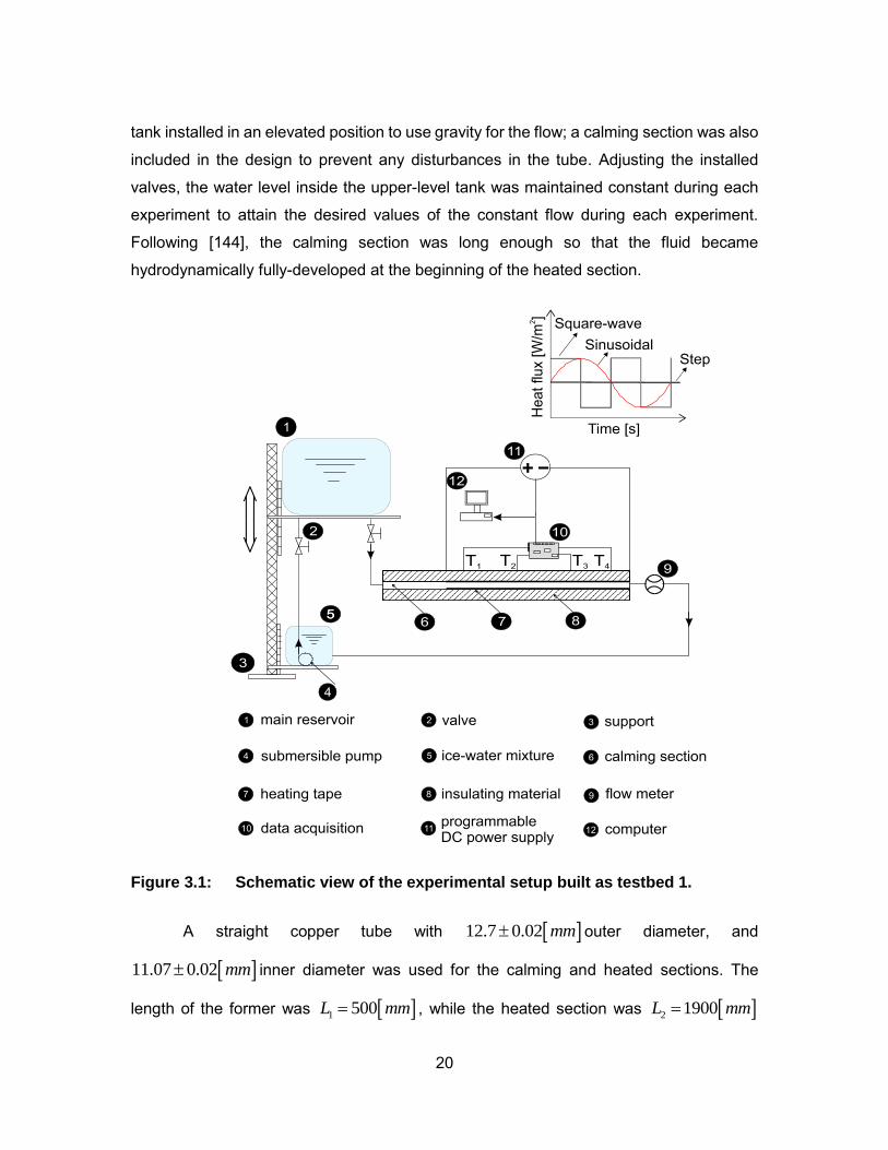
3.1. Testbed 1

The developed experimental setup to investigate steady flow under a time-

dependent heat flux is shown schematically in Figure 3.1. Some pictures of the actual

testbed are also presented in Figure 3.2. The fluid, distilled water, flowed down from a

20

tank installed in an elevated position to use gravity for the flow; a calming section was also

included in the design to prevent any disturbances in the tube. Adjusting the installed

valves, the water level inside the upper-level tank was maintained constant during each

experiment to attain the desired values of the constant flow during each experiment.

Following [144], the calming section was long enough so that the fluid became

hydrodynamically fully-developed at the beginning of the heated section.

Figure 3.1: Schematic view of the experimental setup built as testbed 1.

A straight copper tube with 12.7 0.02 mm outer diameter, and

11.07 0.02 mm inner diameter was used for the calming and heated sections. The

length of the former was 1 500L mm , while the heated section was 2 1900L mm

21

long. Two flexible STH062-120 heating tapes, Omega, were wrapped around the entire

heated section. Four T-type thermocouples were mounted on the heated section at axial

positions in [mm] of T1(300), T2(600), T3(1000), and T4(1700) from the beginning of the

heated section to measure the wall temperature. In addition, two T-type thermocouples

were inserted into the flow at the inlet and outlet of the test section to measure the bulk

temperatures of the distilled water. The heating tapes were connected in series, while

each was 240 V and 940 W . It should be noted that a thin layer of thermal paste was

used between the heaters and the tube to decrease the thermal contact resistance.

(a)

(b)

(c)

(d)

Upper tank

Adjusting

valve

Thermal paste

Copper tube with thermal paste

Thermocouples

Tape heaters

22

(e)

(f)

Figure 3.2: Components of the developed testbed to investigate constant flow under dynamic heat flux: (a) main reservoir (b): copper tube covered with thermal paste (c): flexible heaters wrapped around the tube (d): Insulated tube (e): flow meter (f): DAQ system and power supplies.

Data measurement implemented every 0.1 [s], and each experiment ran for 30

[min]. To apply the time-dependent power on the heated section, two programmable DC

power supplies (Chroma, 62012P-100-50 and 62012P-80-60, USA) were linked in a

master and slave fashion, and connected to the tape heaters. The maximum possible

power was 300 W . To reduce heat losses to the surroundings, a thick layer (5[cm]) of

fiber-glass insulating blanket was wrapped around the entire test section including calming

and heated sections. After the flow passed through the test section, the flow rate was

measured by a precise micro paddlewheel flow meter, FTB300 series Omega. Finally, the

fluid returned to the surge tank which was full of ice-water mixture. As a result, the fluid

was cooled down, and then was pumped back to the main tank at the upper level. All the

thermocouples were connected to a data acquisition system composed of a chassis (NI

cDAQ-9174) and an NI 9213 module; all these components were supplied by National

Instrument. The programmable DC power supplies were controlled via standard LabVIEW

software (National Instrument), to apply the time-dependent powers. As such, different

unsteady cycles were attained by applying three different scenarios for the imposed

power: i) step; ii) sinusoidal; and iii) square-wave. As such, real-time data were obtained

for transient thermal characteristics of the system over such cycles. The experimental

results obtained by testbed 1 are presented in graphical forms in Appendix D, and tabular

forms in Section 3.5.

23

3.2. Test-bed 2

A schematic of testbed 2 is depicted in Figure 3.3. This testbed was developed to

investigate the thermal characteristics of time-dependent flow under time-varying heat

fluxes. As such, a controllable variable-speed peristaltic pump (V6/YZ1515x, Baoding

Shenchen Precision Pump, China) was utilized to apply different patterns of flow inside

the tube. The speed range of the pump was 0.1-600 rpm, and flow rate range was

0.000067-2280ml/min. The pump had various external control modes for option, and also

had programmable external control mode. It supported RS232 and RS485 communication

interfaces as well as standard MODBUS communication protocol, and achieved external

control under different conditions. The technical specifications of the pump are presented

in Table 3.2.

Figure 3.3: A schematic view of testbed 2.

24

Besides, pictures of the single- and variable-speed pumps used in testbeds 1 and

2, respectively, are presented in Figure 3.4.

(a)

(b)

Figure 3.4: (a) Single-speed and (b) variable-speed pumps used in

testbed 1 and 2, respectively.

An AC clamp meter (FLUKE, I 200s) was also connected to the pump and the

LabVIEW interface to monitor the pump power consumption instantaneously. The water-

ice tank was also replaced by a chiller (Cole-Parmer Polystat standard 9.5L heated bath)

to cool down the fluid after passing through the heated section.

Table 3.2: Technical specifications of the utilized variable-speed pump.

Technical specification: Value/range

Flow rate 0.000067-2280ml/min

Speed range 0.1-600rpm

Speed resolution 0.01rpm

Flow rate resolution 0.001μl

25

Flow rate accuracy ±0.5%

Back suction angle 0-360°

Output pressure 0.1Mpa ( 0.86-1.0mm wall thickness tubing）

0.1-0.27Mpa ( 1.6-2.4mm wall thickness tubing) Motor type Stepper motor

Circuit system Shenchen-V-CIR

Operating system Shenchen-V-EMB

Display 4.3 inch industrial grade true color LCD screen

Control method Touch screen and membrane keypad

External cont. signal 0-5V, 0-10V, 4-20mA for option

Start/stop Passive switch signal, such as: foot pedal

Direction signal Active switch signal: 5V, 12V, 24V for option

Communication RS232 and RS485, support MODBUS protocol

RTU) mode Output interface Output motor working status

Drive dimension 260 155 230mm ( L W H)

Drive weight 5.12kg

Power consumption <50W

Environment

temperature

0-40℃

Relative humidity <80%

IP rate IP31

26

A user-friendly interface was developed in LabVIEW connecting to the DAQ

system, power supplies and the pump. The developed analytical models were written as

MATLAB codes and coupled with the LabVIEW interface. In this case, LabVIEW called

the MATLAB functions to evaluate/apply the required flow inside the tube based on the

imposed heat flux. Testbed 2 was used as a proof-of-concept demonstration as a tool to

maintain the temperature of the components generating time-varying thermal loads at a

desired value. Below is a brief description of how one can work with the developed setup.

3.2.1. Time-varying load

Different types of variable thermal load (heat flux) were imposed on the system: i)

step, ii) sinusoidal, iii) square-wave, and iv) driving cycles. There was a module in the

developed interface that enabled one to select between different scenarios to apply the

heat flux. The interface then would command the power supplies to impose the heat flux

on the heaters wrapped around the tube based on the specified load.

3.2.2. Target temperature

As mentioned before, the temperature of the tube was measured at 4 positions on

the tube. Since the imposed heat flux was a function of time, the tube-surface temperature

varied with time at any position along the tube. In addition, the temperature of the tube

increased towards the downstream of the flow, as the bulk-fluid temperature raised in this

direction. If one keeps the temperature at any location constant, then it will be maintained

constant at any position along the tube. In this study, we tried to keep the temperature

constant at T4, as this was the hottest location between all the thermocouples along the

tube.

3.2.3. Coolant flow rate

Based on the imposed heat flux and the targeted temperature, the LabVIEW

interface commanded the pump to apply the required instantaneous flow rate. Two

cooling-scenarios might be considered to control the pump:

27

Proactive cooling: the flow rate was calculated based on the developed analytical

models [145–147]. The interface then commanded the pump to apply the flow inside the

tube with the calculated magnitude. Note that no temperature feedback was used for this

scenario, and pump modulation was only based on the applied power.

Active cooling: high and low set points around the target temperature were

defined (by the user). The pump was then turned on/off by sensing the T4 temperature,

i.e. temperature feedback control. As such, when T4 hit the maximum temperature, the

user interface turned the pump on to work with the maximum capacity. Likewise, when the

temperature went down below the low set point value the interface turned the pump off.

Therefore, the surface temperature swung between high and low temperatures around the

target temperature.

3.2.4. Data acquisition

The data acquisition system consisted of a chassis (NI cDAQ-9174) and four

modules: NI 9213, NI 9205, NI 9225, and 9263. The module NI 9213 was used to record

the temperature data, i.e., four surface temperatures, inlet and outlet temperatures. The

module 9205 was connected to the clamp meter to measure the current of the variable-

speed pump; module NI 9225 measured the voltage of the pump. In addition, NI 9263 was

the voltage modulator to control the pump; this module commanded the pump by voltage

output to apply the required flow rate over a cycle.

3.3. Testbed 3

The components of testbed 3 were the same as those used in testbed 2 except

the test section. A cold plate was used as the test section in testbed 3, see Figure 3.5.

The cold plate consisted of an aluminum heat spreader (152mm89mm13mm), and a U-

shaped 3/8'' copper tube. A tape heater, DHT 101040LD Omega, was wrapped around

the cold plate to mimic the heat generating components mounted on the cold plate. The

heater was 120 volt and 5.2 amps. It should be noted that a thin layer of thermal paste

was used on the cold plate before wrapping the heater to decrease the thermal resistance

between the heater and the cold plate. The cold plate and heater were then wrapped in a

28

fiber-glass blanket. The assembly was wrapped in an aluminum foil, and then insulated

by 2'' rigid polystyrene plates. Two T-type thermocouples were mounted on tube at axial

positions in [mm] of T1 [100], and T2 [230] from inlet to measure the wall temperature. In

addition, inlet and outlet temperatures were also measured by two T-type thermocouples.

All other components including pump, chiller, and DAQ system were the same as those

used in testbed 2.

(a)

(b)

(c)

(d)

Thermocouple

s

inlet

outlet

Thermal paste

Tape heater Fiber-glass

insulation

Aluminum

foil

29

(e)

Figure 3.5: Pictures of testbed 3 (a) location of thermocouples on the tube (b) cold plate covered with thermal paste (c) tape heater wrapped around the cold plate (d) fiber-glass and aluminum foils around the cold plate and heater assembly (e) test section in a polystyrene box.

Schematic 3D view and exploded view of testbed 3 are also shown in Figure 3.6.

(a)

(b)

Figure 3.6: 3D schematic and exploded views of testbed 3

Polystyrene

plates

Fiber-glass

insulation

Cold plate

Polystyrene plate

Cold plate

30

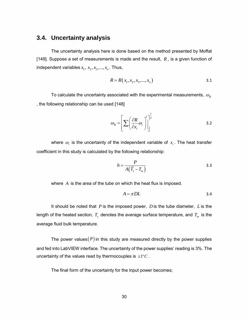
3.4. Uncertainty analysis

The uncertainty analysis here is done based on the method presented by Moffat

[149]. Suppose a set of measurements is made and the result, R , is a given function of

independent variables1 2 3, , ,..., nx x x x . Thus,

1 2 3, , ,..., nR R x x x x 3.1

To calculate the uncertainty associated with the experimental measurements, R

, the following relationship can be used [148]

12 2

R i

i

R

x

3.2

where i is the uncertainty of the independent variable of

ix . The heat transfer

coefficient in this study is calculated by the following relationship:

s m

Ph

A T T

3.3

where A is the area of the tube on which the heat flux is imposed.

A DL 3.4

It should be noted that P is the imposed power, D is the tube diameter, L is the

length of the heated section, sT denotes the average surface temperature, and mT is the

average fluid bulk temperature.

The power values P in this study are measured directly by the power supplies

and fed into LabVIEW interface. The uncertainty of the power supplies’ reading is 3%. The

uncertainty of the values read by thermocouples is 1 C .

The final form of the uncertainty for the input power becomes;

31

1/222 2

s m

s m

T Th P A

h P A T T

3.5

1/22 2

A D L

A D L

3.6

The uncertainty of the Nusselt number is calculated as follows:

1/22 2

Nu h D

Nu h D

3.7

In addition, the uncertainty of the applied micro flow meter was 6%, and the

Reynolds number is calculated based on the flow rate as follows:

4

ReQ

D 3.8

Where Re is the Reynolds number, Q is the flow rate, and is the fluid kinematic

viscosity. Therefore, the uncertainty of Reynolds number is evaluated by the following

relationship.

1/22 2

Re

Re

Q D

Q D

3.9

As such, the accuracy of the measurements and the uncertainties of the derived values are given in Table 3.3.

32

Table 3.3: Summary of calculated experimental uncertainties.

Primary measurements Derived quantities

Parameter Uncertainties Parameter Uncertainties

Q 6% Re 7.6%

P W 3% 2/ /h W m K 9.1%

,s mT T T 1 C Nu 9.3%

3.5. Experimental data

The experimental data logged by LabVIEW are presented in this section in tabular

form. where,

o ino

T T

Lk

3.10

4 inw

T T

Lk

3.11

2

4 tFo

D

3.12

Where 0 and w are the dimensionless outlet and wall temperatures. , , , ,inT L k D , and

t are the inlet temperature, heated-section length, fluid thermal conductivity, fluid thermal

diffusivity, tube diameter, and time, respectively. In addition, sT and mT are the average

surface temperature and fluid bulk temperatures, respectively, defined as follows:

1 2 3 4

4s

T T T TT

3.13

33

2

in outm

T TT

3.14

Where, 1T to

4T are the surface temperatures shown by the thermocouples on tube

surface. inT and outT are the inlet and outlet fluid temperatures.

Table 3.4: Summary of data for outlet temperature under step heat flux

100P W .

Time

s

Fourier Outlet

temperature

C

Dimensionless

outlet temp.

0 0 8.652121 0

20 0.073070866 10.10624 0.040025686

40 0.146141732 12.549207 0.132473018

60 0.219212598 15.109805 0.221365688

80 0.292283465 17.157684 0.293257951

100 0.365354331 18.658171 0.348306028

120 0.438425197 19.732985 0.387906385

200 0.730708661 21.897026 0.469270955

280 1.022992126 22.679554 0.493785602

360 1.315275591 23.075645 0.510085019

440 1.607559055 23.305574 0.518609397

520 1.89984252 23.444714 0.522274152

34

600 2.192125984 23.583965 0.525038826

680 2.484409449 23.687489 0.530378466

760 2.776692913 23.749674 0.533154528

840 3.068976378 23.82859 0.533630928

920 3.361259843 23.888025 0.526468097

1000 3.653543307 23.948458 0.533630928

1080 3.945826772 24.001013 0.530049513

1160 4.238110236 24.052935 0.530049513

1240 4.530393701 24.108883 0.530049513

1320 4.822677165 24.158482 0.526468097

1400 5.11496063 24.231794 0.530049513

1480 5.407244094 24.302246 0.533630928

1560 5.699527559 24.374794 0.537212344

1640 5.991811024 24.438641 0.530049513

1720 6.284094488 24.504465 0.530049513

1800 6.576377953 24.563236 0.526468097

Table 3.5: Summary of data for outlet temperature under square-wave power.

Time

s

Fourier Outlet

temperature

C

Dimensionless

outlet

0 0 6.114547 0

35

20 0.073070866 6.126176 0.000238761

40 0.146141732 6.805634 0.014335523

60 0.219212598 9.214728 0.070194361

80 0.292283465 11.522184 0.124762171

100 0.365354331 13.323492 0.167624099

120 0.438425197 15.138761 0.21165505

200 0.730708661 16.401608 0.24313352

280 1.022992126 16.901848 0.257298616

360 1.315275591 16.079029 0.236044347

440 1.607559055 14.32583 0.193032094

520 1.89984252 12.952079 0.163718136

600 2.192125984 13.973857 0.185800237

680 2.484409449 17.077087 0.259586305

760 2.776692913 17.960108 0.281197498

840 3.068976378 15.784777 0.223415798

920 3.361259843 13.815901 0.1775302

1000 3.653543307 13.262111 0.165287823

1080 3.945826772 15.008973 0.201269279

1160 4.238110236 17.755644 0.268896863

1240 4.530393701 17.782726 0.267653539

1320 4.822677165 15.10263 0.203215611

1400 5.11496063 13.863958 0.1729659

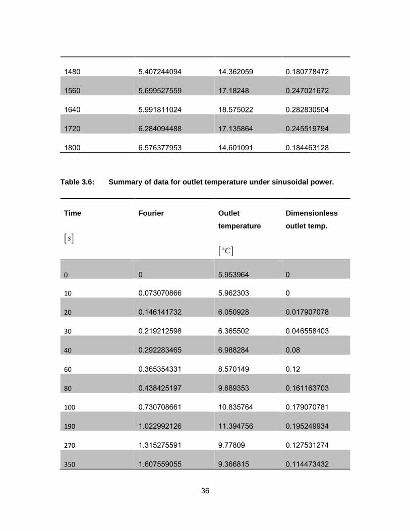
36

1480 5.407244094 14.362059 0.180778472

1560 5.699527559 17.18248 0.247021672

1640 5.991811024 18.575022 0.282830504

1720 6.284094488 17.135864 0.245519794

1800 6.576377953 14.601091 0.184463128

Table 3.6: Summary of data for outlet temperature under sinusoidal power.

Time

s

Fourier Outlet

temperature

C

Dimensionless

outlet temp.

0 0 5.953964 0

10 0.073070866 5.962303 0

20 0.146141732 6.050928 0.017907078

30 0.219212598 6.365502 0.046558403

40 0.292283465 6.988284 0.08

60 0.365354331 8.570149 0.12

80 0.438425197 9.889353 0.161163703

100 0.730708661 10.835764 0.179070781

190 1.022992126 11.394756 0.195249934

270 1.315275591 9.77809 0.127531274

350 1.607559055 9.366815 0.114473432

37

430 1.89984252 11.099916 0.177148564

500 2.192125984 12.621054 0.234825758

580 2.484409449 12.255813 0.217096104

660 2.776692913 10.356788 0.149979658

740 3.068976378 9.57959 0.123023525

820 3.361259843 11.073767 0.17908679

900 3.653543307 12.843814 0.23272293

980 3.945826772 12.436004 0.223319207

1060 4.238110236 10.52688 0.153819796

1140 4.530393701 9.737215 0.121445661

1220 4.822677165 11.222397 0.174943128

1300 5.11496063 12.977089 0.238186666

1700 5.407244094 13.130026 0.242722816

1740 5.699527559 13.231096 0.223818385

1760 5.991811024 13.042304 0.210056321

1780 6.284094488 12.701344 0.208587482

1800 6.576377953 12.280485 0.187907078

38

Table 3.7: Summary of data obtained for wall temperature (4T ) under step wall

heat flux case.

Time

s

Fourier Surface

temperature

C

Dimensionless

surface temp.

0 0 10.68254 0.047731124

10 0.073070866 14.96912 0.164758205

20 0.146141732 18.72503 0.272042099

30 0.219212598 21.89111 0.357101822

40 0.292283465 24.37288 0.424357089

60 0.365354331 26.20711 0.475896056

80 0.438425197 27.38911 0.509310774

100 0.730708661 29.80251 0.578768473

190 1.022992126 30.73983 0.601890396

270 1.315275591 31.23809 0.617243015

350 1.607559055 31.51533 0.625103644

430 1.89984252 31.71952 0.629714799

500 2.192125984 31.8814 0.632464941

580 2.484409449 32.02506 0.637677967

660 2.776692913 32.11748 0.64064652

740 3.068976378 32.21215 0.64052241

820 3.361259843 32.30006 0.64052241

39

900 3.653543307 32.37025 0.641624384

980 3.945826772 32.4381 0.64052241

1060 4.238110236 32.50194 0.64052241

1140 4.530393701 32.57132 0.64052241

1220 4.822677165 32.62973 0.64052241

1300 5.11496063 32.69118 0.64052241

1700 5.407244094 32.77278 0.64052241

1740 5.699527559 32.84833 0.64052241

1760 5.991811024 32.91961 0.64052241

1780 6.284094488 32.97911 0.647409748

1800 6.576377953 33.0427 0.64052241

Table 3.8: Summary of data obtained for wall temperature ( 4T ) under

sinusoidal heat flux case.

Time

s

Fourier Surface

temperature

C

Dimensionless

surface temp.

0 0 5.594989 0

10 0.073070866 6.427629 0.052436

20 0.146141732 7.966392 0.123565

30 0.219212598 9.409614 0.172585

40

40 0.292283465 10.74359 0.221282

60 0.365354331 13.00501 0.251245

80 0.438425197 14.69914 0.291258

100 0.730708661 15.84321 0.348339

190 1.022992126 15.63427 0.347084

270 1.315275591 12.82175 0.236538

350 1.607559055 12.89849 0.240957

430 1.89984252 16.28808 0.362958

500 2.192125984 18.39426 0.441588

580 2.484409449 17.04655 0.388672

660 2.776692913 13.74689 0.271393

740 3.068976378 13.14058 0.250557

820 3.361259843 16.20562 0.36288

900 3.653543307 18.73777 0.44381

980 3.945826772 17.33389 0.398733

1060 4.238110236 14.01521 0.278752

1140 4.530393701 13.37528 0.25174

1220 4.822677165 16.40709 0.360628

1300 5.11496063 18.91915 0.450997

1700 5.407244094 19.08217 0.450885

1740 5.699527559 18.86472 0.431254

1760 5.991811024 18.36598 0.422145

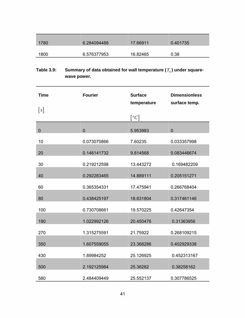
41

1780 6.284094488 17.66911 0.401735

1800 6.576377953 16.82465 0.38

Table 3.9: Summary of data obtained for wall temperature (4T ) under square-

wave power.

Time

s

Fourier Surface

temperature

C

Dimensionless

surface temp.

0 0 5.953983 0

10 0.073070866 7.60235 0.033357998

20 0.146141732 9.814568 0.083446674

30 0.219212598 13.443272 0.169482209

40 0.292283465 14.889111 0.205151271

60 0.365354331 17.475941 0.266768404

80 0.438425197 18.631804 0.317461146

100 0.730708661 19.570225 0.42647354

190 1.022992126 20.450476 0.31363956

270 1.315275591 21.75922 0.268109215

350 1.607559055 23.368286 0.402929338

430 1.89984252 25.126925 0.452313167

500 2.192125984 25.36282 0.38258162

580 2.484409449 25.552137 0.307786525

42

660 2.776692913 23.910202 0.276681882

740 3.068976378 22.447247 0.399664376

820 3.361259843 21.218746 0.453461465

900 3.653543307 20.253191 0.408928591

980 3.945826772 19.710888 0.283007641

1060 4.238110236 19.277061 0.401003539

1140 4.530393701 18.847506 0.459296426

1220 4.822677165 18.546677 0.411503008

1300 5.11496063 18.338228 0.317037823

1700 5.407244094 18.185852 0.290964782

1740 5.699527559 18.839071 0.411458192

1760 5.991811024 20.624666 0.464826681

1780 6.284094488 22.015427 0.412749603

1800 6.576377953 23.192247 0.317488078

Table 3.10: Range of dimensionless parameters in the experiments

Parameter Reynolds number Prandtl number Fourier number Nusselt number

Range 100-1500 1.8-6.5 0-10 0-8

43

Table 3.11: Range of dimensional parameters in the experiments

Parameter Surface

temperature

C

Outlet

temperature

C

Inlet

temperature

C

Time

s

Power

W

Flow rate

/ minml

Range 10-100 20-90 0-10 0-1800 0-800 0-800

44

Chapter 4. Summary of Contributions

The results of this study are published in four journal papers. A summary of the

presented results is reported below.

4.1. Unsteady laminar forced-convective tube flow under dynamic time-dependent heat flux

A new analytical model was developed for steady tube flow under dynamic time-

dependent heat flux. The solution to the time dependent energy equation for a step heat

flux boundary condition was generalized for arbitrary time variations in surface heat flux

using a Duhamel’s integral technique. A sinusoidal heat flux was considered as an

example, and closed-form relationships were proposed for (i) temperature distribution

inside the fluid, (ii) fluid bulk temperature, and (iii) Nusselt number. For the first time, a

new definition was introduced for the Nusselt number, i.e. cyclic fully developed Nusselt

number. Such Nusselt number is associated with the thermally developed region where

the Nusselt number does not vary with axial location but is arbitrary in time. It was shown

that the temperature inside the fluid varies with the angular frequency of the imposed heat

flux. Fluctuations happen around the response for the step heat flux boundary condition.

It was shown that the amplitude of temperature fluctuations decreases towards the

centerline of the tube, which is attributed to the increase in thermal inertia towards the

center of the tube. At any given axial position there is an initial transient period, which can

be considered as pure conduction, i.e. the short time response. However, each axial

position shows steady oscillatory behavior at the long-time response when convection

begins. The analytical results show that at two limiting cases the temperature response

approaches that of step heat flux: (i) heat flux with zero angular frequency and (ii) heat

flux with very high angular frequency. The latter is called “fast transient”; for such rapid

transient the fluid does not follow the details of the heat flux, and yields the response of

step heat flux. This is attributed to the thermal inertia of the fluid. Time- and space-

averages of the Nusselt number were obtained, along with the optimum angular frequency

45

to maximize the Nusselt number. It was also seen that conventional models deviate

considerably from the newly developed transient results. The proposed analytical models

were verified numerically, and the maximum difference was found to be around 5%.

4.2. Unsteady internal forced-convective flow under dynamic time-dependent boundary temperature

The results of this study are presented in Appendix B. A new full-time model was

developed for steady tube flow under dynamic surface temperature. Using Duhamel’s

theorem, closed-form solutions were developed to predict (i) temperature distribution

inside the fluid, (ii) wall heat flux, and (iii) Nusselt number. Both circular tube and parallel

plate geometries were considered, and the proposed relationships can be used for both

configurations. It was shown that for an imposed cyclic wall temperature, the fluid

temperature oscillates around the associated response for the step surface temperature.

Fluctuations occur with the angular frequency that the system is excited with. The shift

between the peaks of the temperature profiles at different radial positions shows a

“thermal lag” (phase shift) for the fluid flow, which increases towards the centerline of the

tube. This thermal lag is attributed to the thermal inertia of the fluid. The phase lag between

the imposed temperature and the heat flux was obtained, and presented as an easy-to-

use relationship. It was noted that the Nusselt number experiences discontinuities, soaring

to plus infinity and then returning from minus infinity. These excursions occur when the

wall and fluid bulk temperature are equal but the heat flux is not zero. In fact, the Nusselt

number loses its significance at these points. In addition, it was observed that when the

angular frequency of the imposed surface temperature is very high, the fluid does not

follow the imposed transient, and yields the response for step wall temperature. The

amplitude of temperature fluctuations inside the tube is a function of the imposed

frequency. At very high and small values of angular frequency, the amplitude approaches

zero, i.e. step wall temperature response. Finally, an arbitrary time-dependent

temperature was imposed on the tube wall, and the fluid response was obtained using a

superposition technique. The analytical results were verified numerically using ANSYS

Fluent.

46

4.3. Optimal unsteady convection over a cycle for arbitrary unsteady flow under dynamic thermal load

The results of this study are presented in Appendix C. A new analytical model was

presented to predict the thermal characteristics of a tube flow with arbitrary unsteadiness

in flow under arbitrary time-dependent heat flux. Exact relationships were obtained to find

(i) the temperature distribution for the fluid; (ii) the fluid bulk temperature, and (iii) the local

and time averaged Nusselt number. New compact relationships were proposed for the

thermal entrance length and the cyclic fully-developed Nusselt number. It was shown that

the period of the Nusselt number oscillations is the least common multiple of the periods

of the imposed harmonic heat flux and the pulsating flow. For the first time, a new

definition, cut-off angular frequency, was proposed to set a criterion for “fast” transients.

As such, when the angular frequency of the imposed heat flux is beyond the cut-off angular

frequency, the fluid feels the heat flux as constant at the average value. A relationship was

obtained for the dimensionless cut-off angular frequency of pulsating flow, beyond which

the heat transfer does not feel the pulsation. The dimensionless cut-off frequency is a

function of pulsation angular frequency, channel geometry, and fluid thermal diffusivity. It

was shown that the Nusselt number is a function of the imposed heat flux, and the fluid

pulsation frequency. As a result, the Nusselt number can be altered by changing the

frequency of the imposed heat flux or fluid pulsation. Optimum flow patterns that can

increase the Nusselt number over a duty cycle were obtained, i.e. an optimal pulsating

flow velocity with optimum frequency that enhances the time averaged Nusselt number by

up to 27%. The model was presented for a general time-dependent heat flux and fluid

flow, however, sinusoidal heat flux and fluid flow were considered as examples for

presenting the closed-form relationships. Thermal lag inside the system was found to be

a function of the angular frequency of the imposed heat flux and pulsating flow. The

developed models show that downstream of the channel, the pulsation effects decrease,

as a result, the heat transfer enhancement drops. The optimum frequency depends on the

angular frequency of the imposed heat flux. In other words, for an imposed harmonic wall

heat flux, there is an optimum value for the pulsation frequency which maximizes the heat

transfer enhancement. Finally, it is indicated that the time averaged Nusselt number of

pulsating flow is equal to that of steady flow over a period of fluctuation.

47

4.4. Temperature-aware time-varying convection over a cycle for a given system thermal-topology

An experimental study was implemented to investigate the thermal behavior of a

steady fully-developed tube flow under time-dependent heat fluxes. To simulate duty

cycles three different transient scenarios were implemented: (i) step; (ii) sinusoidal; and

(iii) square-wave time-varying thermal loads. An experimental testbed was developed as

a proof-of-concept demonstration for efficient dynamic cooling. The setup consists of (i)

programmable power supplies, (ii) programmable pump, (iii) copper tube, and (iv) a data

acquisition system. LabVIEW was used to control the power supplies, and apply the time-

varying heat fluxes. Based on the proposed methodology in Appendix A, analytical

expressions were proposed as closed-form solutions to predict temperature distribution

and Nusselt number under step, sinusoidal, and square wave heat fluxes. The obtained

experimental data were compared with the developed analytical models, with maximum

relative difference of less than 15%. The new definition that was proposed analytically in

Appendix C as cut-off angular frequency was tested/validated experimentally. In addition,

a blending technique was used to propose an all-time model for the Nusselt number under

step wall heat flux. This study was conducted to validate the analytical results obtained

by the author, and it was used, for the first time, as a proof-of-concept demonstration of

efficient variable-capacity liquid cooled systems. In fact, these analyses led to devising

‘‘temperature-aware’’ cooling solutions based on the system thermal topology (power

management) over a given duty cycle. The results of this work provide a platform for the

design, validation and building of new smart thermal management systems that can

actively and proactively control the cooling systems of APEEMs and similar applications.

The results of this study are presented in Appendix D.

48

Chapter 5. Conclusions and Future Works

5.1. Conclusion

In this thesis, new analytical models are presented to predict the thermal

characteristics of a cooling system with unsteady flow under time-dependent heat flux. It

is shown that when a system is excited by a harmonic heat flux, the temperature inside

the system is fluctuating with the same angular frequency. In addition, a thermal lag is

observed between the applied heat flux, and the temperature response. A fully-developed

cyclic Nusselt number is defined which does not vary with axial distance, but arbitrary with

time. It is noted that the fluctuations occur around the response for the time-averaged heat

flux.

Finally, an experimental study is performed to analyze the thermal behavior of a

tube flow under an arbitrary time-dependent heat flux. Several forms of heat flux are taken

into consideration including step, sinusoidal, and square wave. It is shown that there is an

excellent agreement between the obtained experimental data and those predicted by the

developed models.

The question “whether the flow pulsation increases or reduces the heat transfer

rate of convective cooling systems under time dependent thermal load?” is answered here

as follows: “the time averaged Nu number of pulsating flow is equal to that of steady flow

over a period of fluctuation.

Several case studies are also considered to address the following question “how

the thermal characteristics of the dynamic cooling systems vary over a duty cycle?”. The

imposed heat flux (thermal load) is the dominant parameter that characterizes the thermal

behavior of a cooling system. In other words, all the thermal characteristics of a transient

system are a function of the imposed heat flux. For a sinusoidal heat flux, the temperature

varies sinusoidally while for a square-wave load the temperature follows the same pattern.

49

As a result of this work, a new model is developed that predicts the minimum

required flow rate instantaneously to maintain the temperature at a given level under an

arbitrary time-dependent heat flux. As such, thermal stresses within the heat generating

components will be reduced and their durability will increase remarkably. The developed

model also predicts the minimum cooling demand of a system under a given heat flux

based on the set point for the temperature. The results of this study provide a platform to

devise efficient variable-capacity next-generation heat exchange devices for a variety of

engineering applications. Compared to conventional steady-state designs, the developed

model can lead to up to 50% energy saving while maintaining the temperature at the

desired value.

5.2. Future Work

The following research directions can be considered as the continuation of this

dissertation:

Extend the analysis to hydrodynamically developing region. The results of this

study are presented for slug flow and fully-developed flow cases. However,

consideration of hydrodynamicaaly developing region can be a good addition to

this work.

Investigate the effect of interrupted wall heating. In fact, interrupted wall heating

leads to resetting the thermal boundary layer and increases the heat transfer rate.

As such, the heat flux pattern on the wall can be modeled by the models presented

in this dissertation, and best dimensions of interruptions can be obtained.

Extend the analysis to cases with high thermal inertial. There is no analytical

relationship in the literature to predict transient conjugated forced convection.

Investigate the effects of dynamic thermal load on mixed convection. There is no

study in literature on effects of time-varying thermal load on mixed convection and

natural convection.

Investigate the effect of tube surface features, e.g. roughness, grooves, or fins on

transient forced convection under a dynamic thermal load.

50

References

[1] Bennion, K., and Thornton, M., 2010, “Integrated vehicle thermal management for advanced vehicle propulsion technologies,” SAE Tec. Pap. 2010-01-0836, pp. 1–15.

[2] Boglietti, A., Member, S., Cavagnino, A., Staton, D., Shanel, M., Mueller, M., and Mejuto, C., 2009, “Evolution and modern approaches for thermal analysis of electrical machines,” IEEE Trans. Ind. Electron., 56(3), pp. 871–882.

[3] Canders, W.-R., Tareilus, G., Koch, I., and May, H., 2010, “New design and control aspects for electric vehicle drives,” 14th International Power Electronics and Motion Control Conference (EPE-PEMC), Ohrid, Macedonia, pp. 1–8.

[4] Johnson, R. W., Evans, J. L., Jacobsen, P., Thompson, J. R. R., and Christopher, M., 2004, “The changing automotive environment: high-temperature electronics,” IEEE Trans. Electron. Packag. Manuf., 27(3), pp. 164–176.

[5] Mi, C., Peng, F. Z. ., Kelly, K. J. ., Keefe, M. O. ’, and Hassani, V., 2008, “Topology, design, analysis and thermal management of power electronics for hybrid electric vehicle applications,” Int. J. Electr. Hybrid Veh., 1(3), pp. 276–294.

[6] Garrison, J., and Webber, M., 2012, “Optimization of an integrated energy storage scheme for a dispatchable wind powered energy system,” ASME 2012 6th International Conference on Energy Sustainability, Parts A and B San Diego, California, USA, pp. 1009–1019.

[7] Garrison, J., and Webber, M., 2011, “An integrated energy storage scheme for a dispatchable solar and wind powered energy system and analysis of dynamic parameters,” J. Renew. Sustain. Energy, 3(4), pp. 1–11.

[8] Agyenim, F., Hewitt, N., Eames, P., and Smyth, M., 2010, “A review of materials, heat transfer and phase change problem formulation for latent heat thermal energy storage systems (LHTESS),” J. Renew. Sustain. Energy Rev., 14(2), pp. 615–628.

[9] Kurklo, A., 1998, “Energy storage applications in greenhouses by means of phase change materials (PCMs): a review,” J. Renew. Energy, 13(1), pp. 89–103.

[10] Sharma, A., Tyagi, V. V., Chen, C. R., and Buddhi, D., 2009, “Review on thermal energy storage with phase change materials and applications,” J. Renew. Sustain. Energy Rev., 13(2), pp. 318–345.

51

[11] Tang, Q., Gupta, S. K. S., and Varsamopoulos, G., 2008, “Energy-efficient thermal-aware task scheduling for homogeneous high-performance computing data centers: a cyber-physical approach,” IEEE Trans. Parallel Distrib. Syst., 19(11), pp. 1458–1472.

[12] Bash, C., Patel, C., and Sharma, R., 2003, “Efficeint thermal management of data centers-immediate and long-term research needs,” J. HVAC&R Res., 9(2), pp. 137–152.

[13] Beloglazov, A., Abawajy, J., and Buyya, R., 2012, “Energy-aware resource allocation heuristics for efficient management of data centers for Cloud computing,” J. Futur. Gener. Comput. Syst., 28(5), pp. 755–768.

[14] Beloglazov, A., and Buyya, R., 2010, “Energy efficient resource management in virtualized Cloud data centers,” 2010 10th IEEE/ACM Int. Conf. Clust. Cloud Grid Comput., pp. 826–831.

[15] Chen, Y., Gmach, D., Hyser, C., Wang, Z., Bash, C., Hoover, C., and Singhal, S., 2010, “Integrated management of application performance, power and cooling in data centers,” IEEE Netw. Oper. Manag. Symp. (NOMS 2010), pp. 615–622.

[16] Crawford, C., 2005, “Balance of power: dynamic thermal mangement for Internet data centers,” IEEE Internet Comput., 9(1), pp. 42–49.

[17] Anandan, S., and Ramalingam, V., 2008, “Thermal management of electronics: A review of literature,” Int. J. Therm. Sci., 12(2), pp. 5–26.

[18] Gurrum, S. P. S. P., Suman, S. K., Shivesh, K., Joshi, Y. K., and Fedorov, A. G., 2004, “Thermal Issues in Next-Generation Integrated Circuits,” IEEE Trans. Device Mater. Reliab., 4(4), pp. 709–714.

[19] Scott Downing, R., and Kojasoy, G., 2002, “Single and two-phase pressure drop characteristics in miniature helical channels,” J. Exp. Therm. Fluid Sci., 26(5), pp. 535–546.

[20] Joshi, Y., and Wei, X., 2005, “Micro and meso scale compact heat exchangers in electronics thermal management-a review,” Enhanced, Compact and Ultra-Compact Heat Exchangers: Science, Engineering and Technology (CHE-2005), pp. 162–179.

[21] Wankhede, M., Khaire, V., and Goswami, A., 2007, “Evaluation of cooling solutions for outdoor electronics,” 13th International Conference on Thermal Investigation of ICs and Systems, ©EDA Publishing, Budapest, Hungary, pp. 1–6.

[22] Jahkonen, J., Puolakka, M., and Halonen, L., 2013, “Thermal management of outdoor LED lighting systems and streetlights variation of ambient cooling conditions,” J. Illum. Eng. Soc. North Am., 9(3), pp. 155–176.

52

[23] Christensen, A., Ha, M., and Graham, S., 2007, “Thermal management methods for compact high power LED arrays,” 7th International Conference on Solid State Lighting, SPIE UK, San Diego, California, USA, pp. 1–19.

[24] BCCResearch, 2014, The Market for Thermal Management Technologies, Wellesley, MA, USA.

[25] Garimella, S. V, Yeh, L., and Persoons, T., 2012, “Thermal management challenges in telecommunication systems and data centers,” CTRC Res. Publ., pp. 1–26.

[26] Sawin, J. L., and E. Martinot, 2011, Renewables Bounced Back in 2010, Finds REN21 Global Report.

[27] Ulf Herrmann, and Kearney, D. W., 2002, “Survey of thermal energy storage for parabolic trough power plants,” ASME J. Sol. Energy Eng., 124(2), pp. 145–152.

[28] Garrison, J. B., and E. Webber, M., 2012, “Optimization of an integrated energy storage for a dispatchable wind powered energy system,” ASME 2012 6th International Conference on Energy Sustainability, pp. 1–11.

[29] O’Keefe, M., and Bennion, K., 2007, “A comparison of hybrid electric vehicle power electronics cooling options,” Vehicle Power and Propulsion Conference, pp. 116–123.

[30] Joshi, Y., Kumar, P., Sammakia, B., and Patterson, M., 2012, Energy efficient thermal management of data centers, Springer US, Boston, MA.

[31] Siegel, R., Sparrow, E. M., and Hallman, T. M., 1958, “Steady laminar heat transfer in a circular tube with prescribed wall heat flux,” Appl. Sci. Res. Sect. A, 7(5), pp. 386–392.

[32] Siegel, R., 1959, “Transient heat transfer for laminar slug flow in ducts,” Trans. ASME, 81, pp. 140–142.

[33] Rizika, J. W., 1954, “Thermal lags in flowing systems containing heat capacitors,” Trans. ASME, 76, pp. 411–420.

[34] Rizika, J. W., 1956, “Thermal lags in flowing incompressible fluid systems containing heat capacitors,” Trans. ASME, 78, pp. 1407–1412.

[35] Sparrow, E. M., and Siegel, R., 1958, “Thermal entrance region of a circular tube under transient heating conditions,” Third U. S. National Congress for Applied Mechanics, pp. 817–826.

53

[36] Siegel, R., and Sparrow, E. M., 1959, “Transient heat transfer for laminar forced convection in the thermal entrance region of flat ducts,” Trans. ASME, 81(C), pp. 29–36.

[37] Clarck, J. A., Arpaci, V. S., and Treadwell, K. M., 1958, “Dynamic response of heat exchangers having internal heat sources-Part I,” Trans. ASME, 80, pp. 612–624.

[38] Clark, J. A., and Arpaci, V. S., 1958, “Dynamic response of heat exchangers having internal heat sources- Part II,” Trans. ASME, 80, pp. 625–634.

[39] Siegel, R., 1960, “Heat transfer for laminar flow in ducts with arbitrary time variations in wall tempearture,” Trans. ASME, 82(E), pp. 241–249.

[40] Perlmutter, M., and Siegel, R., 1961, “Unsteady laminar flow in a duct with unsteady heat addition,” Trans. ASME, 83(C), pp. 432–440.

[41] Bonilla, C. F., Busch, J. S., Landau, H. G., and Lynn, L. L., 1961, “Formal heat transfer solutions,” Nucl. Sci. Eng., 9, pp. 323–331.

[42] Perlmutter, M., and R. Siegel, 1961, “Two-dimensional unsteady incompressible laminar duct flow with a step change in wall tempearture,” Int. J. Heat Mass Transf., 3, pp. 94–107.

[43] Siegel, R., and Perlmutter, M., 1963, “Laminar heat transfer in a channel with unsteady flow and wall heating varying with position and time,” Trans. ASME, 85, pp. 358–365.

[44] HSU, C.-J., 1965, “Heat transfer in a round tube with sinusoidal wall heat flux distribution,” J. Am. Inst. Chem. Eng., 11(4), pp. 690–695.

[45] Kays, W. M., and Crawford, M. E., 1993, Convective heat and mass transfer, McGraw-Hill, New York.

[46] Conley, N., Lawal, A., and Mujumdar, A. S., 1985, “An assessment of the accuracy of numerical solutions to the Graetz problem,” J. Int. Commun. Heat Mass Transf., 12, pp. 209–218.

[47] Sucec, J., and Radley, D., 1990, “Unsteady forced convection heat transfer in a channel,” Int. J. Heat Mass Transf., 33(4), pp. 683–690.

[48] Lin, H. T., and Shih, Y. P., 1981, “Unsteady thermal entrance heat transfer of power-law fluids in pipes and plate slits,” Int. J. Heat Mass Transf., 24(9), pp. 1531–1539.

54

[49] Chen, S. C., Anand, N. K., and Tree, D. R., 1983, “Analysis of transient laminar convective heat transfer inside a circular duct,” ASME J. Heat Transf., 105, pp. 922–924.

[50] Barletta, a., and Zanchini, E., 1995, “Laminar forced convection with sinusoidal wall heat flux distribution: axially periodic regime,” J. Heat Mass Transf., 31(1), pp. 41–48.

[51] Astaraki, M. R., Tabari, N. G., and Rudhelepur, a., 2013, “Analytical Solution of Periodic Laminar Forced Convection via Confluent Hypergeometric Function,” J. Thermophys. Heat Transf., pp. 1–5.

[52] Kakac, S., and Yener, Y., 1973, “Exact solution of the transient forced convection energy equation for timewise variation of inlet temperature,” Int. J. Heat Mass Transf., 16, pp. 2205–2214.

[53] Cotta, R. M., Mikhailov, M. D., and Ozisik, M. N., 1987, “Transient conjugated forced convection in ducts with peridically varying inlet temperature,” Int. J. Heat Mass Transf., 30(10), pp. 2073–2082.

[54] Cotta, R. M., and Ozisik, M. N., 1986, “Laminar forced convection inside ducts with periodic variation of inlet temperature,” Int. J. Heat Mass Transf., 29(10), pp. 1495–1501.

[55] Hadiouche, a., and Mansouri, K., 2010, “Analysis of the effects of inlet temperature frequency in fully developed laminar duct flows,” J. Eng. Phys. Thermophys., 83(2), pp. 380–392.

[56] Kakac, S., Ding, Y., and Li, W., 1988, “Experimental study on unsteady laminar forced convection in ducts for timewise varying inlet tempearture,” Proceedings of the First World Conference on Experimental Heat Transfer, Fluid mechanics, and Thermodynamics, pp. 1177–1184.

[57] Kakac, S., Li, W., and Cotta, R. M., 1990, “Unsteady laminar forced convection in ducts with periodic variation of inlet temperature,” J. Mech. Des., 112, pp. 913–920.

[58] Sparrow, E. M., and Farias, F. N. De, 1968, “Unsteady heat transfer in ducts with time-varying inlet tempearture and participating walls,” Int. J. Heat Mass Transf., 11, pp. 837–853.

[59] Weigong, L., and Kakac, S., 1991, “Unsteady thermal entrance heat transfer in laminar flow with a periodic variation of inlet temperature,” Int. J. Heat Mass Transf., 34(10), pp. 2581–2592.

55

[60] Siegel, R., 1963, “Forced convection in a channel with wall heat capacity and with wall heating variable with axial position and time,” Int. J. Heat Mass Transf., 6, pp. 607–620.

[61] Olek, S., 1999, “Multiregion Conjugate Heat Transfer,” J. Hybrid Methods Eng., 1, pp. 119–137.

[62] Aleksashenko, V. A., 1968, “Conjugate stationary problem of heat transfer with a moving fluid in a semi-infinite tube allowing for viscous dissipation,” J. Eng. Phys., 14(1), pp. 100–107.

[63] Sucec, J., 1981, “An improved quasi-steady approach for transient conjugated forced convection problems,” Int. J. Heat Mass Transf., 24(10), pp. 1711–1722.

[64] Sucec, J., 1987, “Exact solution for unsteady conjugated heat transfer in the thermal entrance region of a duct,” ASME J. Heat Transf., 109(2), pp. 295–299.

[65] Olek, S., Elias, E., Wacholder, E., and Kaizerman, S., 1991, “Unsteady conjugated heat transfer in laminar pipe flow,” Int. J. Heat Mass Transf., 34(6), pp. 1443–1450.

[66] Sucec, J., 2002, “Unsteady forced convection with sinusoidal duct wall generation: the conjugate heat transfer problem,” Int. J. Heat Mass Transf., 45(8), pp. 1631–1642.

[67] Lin, T. F., and Kuo, J. C., 1988, “Transient conjugated heat transfer in fully developed laminar pipe flows,” Int. J. Heat Mass Transf., 31(5), pp. 1093–1102.

[68] Schutte, D. J., Rahman, M. M., and Faghri, A., 1992, “Transient conjugate heat transfer in a thick-walled pipe with developing laminar flow,” J. Numer. Heat Transf. Part A, 21, pp. 163–186.

[69] Yan, W. M., Tsay, Y. L., and Lin, T. F., 1989, “Transient conjugated heat transfer in laminar pipe flows,” Int. J. Heat Mass Transf., 32(4), pp. 775–777.

[70] Luna, N., Méndez, F., and Mar, E., 2003, “Transient analysis of the conjugated heat transfer in circular ducts with a power-law fluid,” J. Nonnewton. Fluid Mech., 111(2-3), pp. 69–85.

[71] Travelho, J. S., and Santos, W. F. N., 1998, “Unsteady conjugate heat transfer in a circular duct with convection from the ambient and periodically varying inlet temperature,” ASME J. Heat Transf., 120(2), pp. 506–510.

[72] Hadiouche, A., and Mansouri, K., 2010, “Application of integral transform technique to the transient laminar flow heat transfer in the ducts,” Int. J. Therm. Sci., 49(1), pp. 10–22.

56

[73] Kiwan, S. M., and Al-Nimr, M. a., 2002, “Analytical solution for conjugated heat transfer in pipes and ducts,” J. Heat Mass Transf., 38(6), pp. 513–516.

[74] Al-Nimr, M. A., and Ei-Shaarawi, M. A. I., 1992, “Analytical solutions for transient conjugated heat transfer in a parallel plate and circular ducts,” J. Int. Commun. Heat Mass Transf., 19, pp. 869–878.

[75] Khadrawi, A. F., and Al-nimr, M. A., 2003, “A perturbation technique to solve conjugated heat transfer problems in circular ducts,” J. Heat Mass Transf., 39, pp. 125–130.

[76] Luikov, A. V., Aleksashenko, V. A., and Aleksashenko, A. A., 1971, “Analytical methods of solution of conjugated problems in convective heat transfer,” Int. J. Heat Mass Transf., 14, pp. 1047–1056.

[77] Guedes, R. O. C., and Özişik, M. N., 1992, “Conjugated turbulent heat transfer with axial conduction in wall and convection boundary conditions in a parallel-plate channel,” Int. J. Heat Fluid Flow, 13(4), pp. 322–328.

[78] Bilir, S., and Ates, A., 2003, “Transient conjugated heat transfer in thick walled pipes with convective boundary condition,” Int. J. Heat Mass Transf., 46(2), pp. 2701–2709.

[79] Bilir, S., 1995, “Laminar flow heat transfer in pipes including two-dimensional wall and fluid axial conduction,” Int. J. Heat Mass Transf., 38, pp. 1619–1625.

[80] Bilir, S., 2002, “Transient conjugated heat transfer in pipes involving two-dimensional wall and axial fluid conduction,” Int. J. Heat Mass Transf., 45, pp. 1781–1788.

[81] Cotta, R. M., Mikhailov, M. D., and Özişik, M. N., 1987, “Transient conjugated forced convection in ducts with periodically varying inlet temperature,” Int. J. Heat Mass Transf., 30, pp. 2073–2082.

[82] Sucec, J., and Weng, H. Z., 2002, “Unsteady conjugated duct heat transfer solution with wall heating,” J. Thermophys. Heat Transf., 16, pp. 128–134.

[83] Wijeysundera, N. E., 1986, “Laminar forced convection in circular and flat ducts with wall axial conduction and external convection,” Int. J. Heat Mass Transf., 29, pp. 797–807.

[84] Guedes, R. O. C., and Cotta, R. M., 1991, “Periodic laminar forced convection within ducts including wall heat conduction effects,” Int. J. Eng. Sci., 29(5), pp. 535–547.

[85] Karvinen, R., 1988, “Transient conjugated heat transfer to laminar flow in a tube or channel,” Int. J. Heat Mass Transf., 31(6), pp. 1326–1328.

57

[86] Soliman, H. M., and Rahman, M. M., 2005, “Analytical solution of conjugate heat transfer and optimum configurations of flat-plate heat exchangers with circular flow channels,” J. Heat Mass Transf., 42(7), pp. 596–607.

[87] Soliman, H. M., 1984, “Analysis of low-Peclet heat transfer during slug flow in tubes with axial wall conduction,” ASME J. Heat Transf., 106, pp. 782–788.

[88] Barozzi, G. S., and Pagliarini, G., 1985, “A method to solve conjugate heat transfer problems: the case of fully developed laminar flow in a pipe,” ASME J. Heat Transf., 107, pp. 77–83.

[89] Faghri, M., and Sparrow, E. M., 1980, “Simultaneous wall and fluid axial conduction in laminar pipe-flow heat transfer,” ASME J. Heat Transf., 102(58), pp. 58–63.

[90] Papoutsakis, E., and Ramkrishna, D., 1981, “Conjugated Graetz problem-I. General formalism and a class of solid-fluid problems,” J. Chem. Eng. Sci., 36, pp. 1381–1391.

[91] Papoutsakis, E., and Ramkrishna, D., 1981, “Conjugated Graetz problem-II. General formalism and a class of fluid-fluid problems,” J. Chem. Eng. Sci., 36, pp. 1393–1399.

[92] Koshkin, V. K., Kalinin, E. K., Dreitser, G. A., Galitseisky, B. M., and Izosimov, V. G., 1970, “Experimental study of unsteady convective heat transfer in tubes,” Int. J. Heat Mass Transf., 13, pp. 1271–1281.

[93] Kawamura, H., 1977, “Experimental and analytical study of transient heat transfer for turbulent flow in a circular tube,” Int. J. Heat Mass Transf., 20, pp. 443–450.

[94] Barozzi, G. S., and Pagliarini, G., 1984, “Experimental investigation of coupled conduction and laminar convection in a circular tube,” Int. J. Heat Mass Transf., 27(12), pp. 2321–2329.

[95] Watson, E. J., 1983, “Diffusion in oscillatory pipe flow,” J. Fluid Mech., 133, pp. 233–244.

[96] Joshi, C. H., Kamm, R. D., Drazen, J. M., and Slutsky, A. S., 1983, “An experimental study of gas exchange in laminar oscilltory flow,” J. Fluid Mech., 133, pp. 245–254.

[97] Kurzweg, U. H., 1985, “Enhanced heat conduction in oscillating viscous flows within parallel-plate channels,” J. Fluid Mech., 156, pp. 291–300.

[98] West, F. B., and Taylor, A. T., 1952, “The effect of pulsations on heat transfer; turbulet flow of water inside tubes,” J. Chem. Eng. Prog., 48(1), pp. 39–43.

58

[99] Martinelli, R. C., Boelter, L. M. K., Weinberg, E. B., and Yakahi, S., 1943, “Heat transfer to a fluid flowing periodically at low frequencies in a vertical tube,” Trans. ASME, 65, pp. 789–798.

[100] Havemann, H., and Rao, N., 1954, “Heat transfer in pulsating flow,” J. Nat., 174, p. 41.

[101] Darling, G. B., 1959, “Heat transfer to liquids in intermittent flow,” J. Pet., 22, pp. 177–178.

[102] Hwang, M. F., and Dybbs, A., 1983, “Heat transfer in a tube with oscillatory flow,” ASME paper 83-WA/Ht-90, pp. 1–12.

[103] Faghri, M., Javdani, K., and Faghri, A., 1979, “Heat transfer with laminar pulsating flow in a pipe,” J. Lett. Heat Mass Transf., 6(4), pp. 259–270.

[104] R. Siegel, 1987, “Influence of oscillaation diffusion on heat transfer in a uniformly heated channel,” Trans. ASME, 109, pp. 244–249.

[105] Mamayev, V., Nosov, V., and Syromyatnikov, N., 1976, “Investigation of heat transfer in pulsed flow of air in pipes,” J. Heat Transf. Res., 8(3), pp. 111–116.

[106] Hemida, H. N., Sabry, M. N., Abdel-Rahim, A., and Mansour, H., 2002, “Theoretical analysis of heat transfer in laminar pulsating flow,” Int. J. Heat Mass Transf., 45(8), pp. 1767–1780.

[107] Siegel, R., and Perlmutter, M., 1962, “Heat transfer for pulsating laminar duct flow,” ASME J. Heat Transf., 84(2), pp. 111–122.

[108] Mackley, M. R., Tweddle, G. M., and Wyatt, I. D., 1990, “Experimental heat transfer measurement for pulsatile flow in baffled tubes,” J. Chem. Sci. Eng., 45(5), pp. 1237–1242.

[109] Mackley, M. R., and Stonestreet, P., 1995, “Heat transfer and associated energy dissipation for oscialltory flow in baffled tubes,” J. Chem. Sci. Eng., 50(14), p. 1995.

[110] Moschandreou, T., and Zamir, M., 1997, “Heat transfer in a tube with pulsating flow and constant heat flux,” Int. J. Heat Mass Transf., 40(10), pp. 2461–2466.

[111] Kim, S. Y., Kang, B. H., and Hyun, J. M., 1993, “Heat transfer in the thermally developing region of a pulsating channel flow,” Int. J. Heat Mass Transf., 36(17), pp. 4257–4266.

[112] Cho, H. W., and Hyun, J. M., 1990, “Numerical solution of pulsating flow and heat transfer characteristics in a pipe,” Int. J. Heat Fluid Flow, 11(4), pp. 321–330.

59

[113] Zhao, T., and Cheng, P., 1995, “A numerical solution of laminar forced convection in a heated pipe subjected to a reciprocating flow,” Int. J. Heat Mass Transf., 38(16), pp. 3011–3022.

[114] Wommersley, J. R., 1955, “Method for the calculation of velocity, rate of the flow and viscous drag in arteries when the pressure gradient is known,” J. Physiol., 127, pp. 553–563.

[115] Guo, Z., and Sung, H., 1997, “Analysis of the Nusselt number in pulsating pipe flow,” Int. J. Heat Mass Transf., 40(10), pp. 2486–2489.

[116] Habib, M. a., Attya, a. M., Eid, a. I., and Aly, a. Z., 2002, “Convective heat transfer characteristics of laminar pulsating pipe air flow,” J. Heat Mass Transf., 38(3), pp. 221–232.

[117] Gupta, S. K., Patel, R. D., and Ackerberg, R. C., 1982, “Wall heat/mass transfer in pulsatile flow,” J. Chem. Eng. Sci., 37(12), pp. 1727–1739.

[118] Krishnan, K. N., and Sastri, V. M. K., 1989, “Heat transfer in laminar pulsating flows of fluids with tempearture dependent viscosities,” J. Warme Stoffubertragung, 24, pp. 37–42.

[119] Lemlich, R., 1961, “Vibration and pulsation boost heat transfer,” J. Chem. Eng., 68, pp. 171–176.

[120] Lemlich, R., and Hwu, C., 1961, “The effect of acoustic vibration on forced convective heat transfer,” Am. Inst. Chem. Eng., 21, pp. 197–199.

[121] Niida, T., Yoshida, T., Yamashita, R., and Nakayama, S., 1974, “The influence of pulsation on laminar heat transfer in pipes,” J. Heat Transf. Res., 3(3), pp. 19–28.

[122] Shuai, X., Cheng, S., and Antonni, G., 1994, “Pulsation effects on convective heat transfer in the laminar flow of a viscous fluid,” Can. J. Chem. Eng., 72, pp. 468–475.

[123] Yu, J.-C., Li, Z.-X., and Zhao, T. S., 2004, “An analytical study of pulsating laminar heat convection in a circular tube with constant heat flux,” Int. J. Heat Mass Transf., 47(24), pp. 5297–5301.

[124] Brereton, G. J., and Jiang, Y., 2006, “Convective heat transfer in unsteady laminar parallel flows,” J. Phys. Fluids, 18(10), pp. 1–15.

[125] Nield, D. a., and Kuznetsov, a. V., 2007, “Forced convection with laminar pulsating flow in a channel or tube,” Int. J. Therm. Sci., 46(6), pp. 551–560.

[126] Yan, B. H., Yu, L., and Yang, Y. H., 2010, “Forced convection with laminar pulsating flow in a tube,” J. Heat Mass Transf., 47(2), pp. 197–202.

60

[127] Paek, J. W., Kang, B. H., and Hynn, J. M., 1999, “Transient cool-down of a porous medium in pulsating flow,” Int. J. Heat Mass Transf., 42, pp. 3523–3527.

[128] Fu, H. L., Leong, K. C., Huang, X. Y., and Liu, C. Y., 2001, “An experimental study of heat transfer of a porous channel subjected to oscillating flow,” ASME J. Heat Transf., 123, pp. 162–170.

[129] Leong, K. C., and Jin, L. W., 2005, “Heat transfer of oscillating flow and steady flows in a channel filled with an aluminum foam,” Int. J. Heat Mass Transf., 48, pp. 243–253.

[130] Myrum, T. A., Acharya, S., and Inamdar, S., 1997, “Laminar pulsed forced and mixed convection in a vertical isothermal tube,” J. Thermophys. Heat Transf., 11, pp. 423–428.

[131] Bandyopadhyay, S., and Mazumder, B. S., 1999, “Unsteady convective diffusion in a pulsatile flow through a channel,” J. Acta Mech., 134(1), pp. 1–16.

[132] Lee, D., Park, S., and Rot, S. T., 1995, “Heat transfer by oscillating flow in a circular pipe with a sinusoidal wall temperature distribution,” Int. J. Heat Mass Transf., 38(14), pp. 2529–2537.

[133] Lin, T. F., Hawks, K. H., Leidenfrost, W., and Ausgleichsvorg, Z., 1983, “Transient thermal entrance heat transfer in laminar pipe flows with step change in pumping pressure,” J. Wärme - und Stoffübertragung, 17, pp. 201–209.

[134] Lin, T. F., Hawks, K. H., and Leidenfrost, W., 1983, “Unsteady thermal entrance heat transfer in laminar pipe flows with step change in ambient temperature,” J. Wärme - und Stoffübertragung, 17(3), pp. 125–132.

[135] Loudon, C., and Tordesillas, A., 1998, “The use of the dimensionless Womersley number to characterize the unsteady nature of internal flow,” J. Theor. Biol., 191(1), pp. 63–78.

[136] Uchida, S., 1956, “The pulsating viscous flow superposed on the steady laminar motion of incompressible fluid in a circular pipe,” J. Zeitschrift für Angew. Math. und Phys., 7(5), pp. 403–422.

[137] Zhao, T. S., and Cheng, P., 1996, “Oscillatory heat transfer in a pipe subjected a periodically reversing flow,” ASME J. Heat Transf., 118, pp. 592–598.

[138] Zhao, T. S., and Cheng, P., 1996, “Experimental investigations of the onset of turbulence and frictional losses in an oscillatory pipe flow,” Int. J. Heat Fluid Flow, 17, pp. 356–362.

[139] Zhao, T. S., and Cheng, P., 1996, “Oscillatory pressure drops through a woven-screen packed column subjected to a cyclic flow,” J. Cryog., 36, pp. 333–341.

61

[140] Gibson, M. M., and Diakoumakos, E., 1993, “Oscillating turbulent boundary layer on a heated wall,” Ninth Symposium on Turbulent Shear Flows, pp. 16–18.

[141] Ramaprian, B. R., and Tu, S. W., 1981, “Periodic turbulent pipe flow at high frequencies of oscillation,” IUTAM Symposium, pp. 47–58.

[142] Ohmi, M., Usui, T., Tanaka, O., and Toyama, M., 1976, “Pressure and velocity distributions in pulsating turbulent pipe flow,” Bull. JSME, 19(134), pp. 951–957.

[143] Parikh, P. G., Reynolds, W. C., Jaydraman, R., and Carr, L. W., 1981, “Dynamic behavior of an unsteady turbulent boundary layer,” IUTAM Symposium, pp. 35–47.

[144] Incropera, F. P., Dewitt, D. P., Bergman, T. L., and Lavine, A. S., 2007, Introduction to heat transfer, John Wiley & Sons, USA.

[145] Fakoor-Pakdaman, M., Andisheh-Tadbir, M., and Bahrami, M., 2013, “Unsteady laminar forced-convective tube flow under dynamic time-dependent heat flux,” J. Heat Transfer, 136(4), pp. 041706–1–10.

[146] Fakoor-Pakdaman, M., Ahmadi, M., and Bahrami, M., 2014, “Unsteady internal forced-convective flow under dynamic time-dependent boundary temperature,” J. Thermophys. Heat Transf., 28(3), pp. 463–473.

[147] Fakoor-Pakdaman, M., Ahmadi, M., Andisheh-Tadbir, M., and Bahrami, M., 2014, “Optimal unsteady convection over a duty cycle for arbitrary unsteady flow under dynamic thermal load,” Int. J. Heat Mass Transf., 78, pp. 1187–1198.

[148] Fakoor-Pakdaman, M., Ahmadi, M., Andisheh-Tadbir, M., Bahrami, M., (2015) “Temperature-aware time-varying convection over a duty cycle for a given system thermal-topology”, Int. J. Heat Mass Transf., 87, pp. 418–428.

[149] Moffat, R. J., 1988, “Describing the uncertainties in experimental results,” Exp. Therm. Fluid Sci., 1(1), pp. 3–17.

Appendix A

Unsteady internal forced-convective flow under dynamic time-dependent boundary temperature

62

Unsteady Internal Forced-Convective Flow Under DynamicTime-Dependent Boundary Temperature

M. Fakoor-Pakdaman,∗ Mehran Ahmadi,† and Majid Bahrami‡

Simon Fraser University Surrey, British Columbia V3T 0A3, Canada

DOI: 10.2514/1.T4261

A new all-time analytical model is developed to predict transient internal forced-convection heat transfer under

arbitrary time-dependentwall temperature. Slug flow condition is assumed for the velocity profile inside the tube.The

solution to the time-dependent energy equation for a stepwall temperature is generalized for arbitrary time variations

in surface temperature using Duhamel’s theorem. A harmonic boundary temperature is considered, and new

compact closed-form relationships are proposed to predic: 1) fluid temperature distribution; 2) fluid bulk temper-

ature; 3) wall heat flux; and 4) the Nusselt number. An optimum value is found for the dimensionless angular

frequency of the wall temperature to maximize the heat transfer rate of the studied unsteady forced-convective

process. Such dimensionless parameter depends upon the imposed-temperature angular frequency, fluid thermo-

physical properties, and tube geometrical parameters. A general surface temperature is considered, and the

temperature field inside the medium is obtained using a superposition technique. An independent numerical simula-

tion is performed using ANSYS® Fluent. The comparison between the obtained numerical data and the present

analytical model shows good agreement: a maximum relative difference less than 4.9%.

Nomenclature

A = cross-sectional area, Eq. (13), m2

a = half-width of spacing between parallel plates, or circulartube radius, m

cp = heat capacity, J∕kg · K

Fo = Fourier number; αt∕a2J = Bessel function, Eq. (6a)k = thermal conductivity,W∕m · KNu = Nusselt number, ha∕Kn = positive integer, Eq. (6b)p = 0 for parallel plate and 1 for circular tube, Eqs. (3) and (14)Pr = Prandtl number (ν∕α)q�w = dimensionless wall heat flux

Re = Reynolds number, 2Ua∕νr = radial coordinate measured from circular tube center-

line, mT = temperature, KU = velocity magnitude, m∕su = velocity vector, Eq. (2)x = axial distance from the entrance of the heated section, my = normal coordinate measured from centerline of parallel

plate channel, mα = thermal diffusivity, m2∕sγ = function for circular tube [Eq. (6a)] or for parallel plate

[Eq. (6b)]Δφ = thermal lag (phase shift)ζ = dummy X variableη = dimensionless radial/normal coordinate for circular tube

equal to r∕a or for parallel plate equal to y∕aθ = dimensionless temperature; �T − T0�∕ΔTR

λn = eigenvalues, Eq. (6)ν = kinematic viscosity, m2∕s

ξ = dummy Fo variableρ = fluid density, kg∕m3

ψ = arbitrary function of FoΩ = imposed-temperature angular frequency, rad∕sω = dimensionless temperature angular frequency,

Subscripts

m = mean or bulk valueR = reference values = step wall (surface) temperaturew = wall0 = inlet

I. Introduction

D EVELOPING an in-depth understanding of unsteady forced-convection heat transfer is crucial for optimal design and accu-

rate control of heat transfer in emerging sustainable energy applica-tions and next-generation heat exchangers. The origin of thermaltransients in sustainable energy applications include thevariable ther-mal load on 1) thermal solar panels in thermal energy storage (TES)systems [1–3]; 2) power electronics of solar/wind/tidal energy con-version systems [4,5]; and 3) power electronics and electric motor(PEEM) of hybrid electric vehicles (HEVs), electric vehicles (EVs),and fuel cell vehicles (FCVs) [6–9].Solar thermal systems are widely used in solar powerplants and

are being widely commercialized. Solar powerplants have seen about740 MW of generating capacity added between 2007 and the endof 2010, bringing the global total to 1095 MW [5]. Such growth isexpected to continue, as in the United States at least another 6.2 GWcapacity is expected tobe in operation by the endof 2013 [5].However,the growth of such technology is hindered by the inherent variability ofsolar energy subjected to daily variation, seasonal variation, andweather conditions [1,4,10]. To overcome the issue of the intermit-tency,TES systemsare used to collect thermal energy to smooth out theoutput and shift its delivery to a later time. Single-phase sensibleheating systems or latent heat storage systems using phase changematerials are used in TES; transient heat exchange occurs to charge ordischarge the storage material [11]. From the technical point of view,one of the main challenges facing TES systems is designing suitableheat exchangers towork reliably under unsteady conditions [11]: a keyissue that this research attempts to address.To assure reliable performance of electronic components, the

temperature of different components should be maintained below

Received 23 August 2013; revision received 23 November 2013; acceptedfor publication 9 January 2014; published online 21 April 2014. Copyright ©2013 by the American Institute of Aeronautics and Astronautics, Inc. Allrights reserved. Copies of this paper may be made for personal or internal use,on condition that the copier pay the $10.00 per-copy fee to the CopyrightClearance Center, Inc., 222 Rosewood Drive, Danvers, MA 01923; includethe code 1533-6808/14 and $10.00 in correspondence with the CCC.

*Laboratory for Alternative Energy Convection, School of MechatronicSystems Engineering, No. 4300, 250-13450 102nd Avenue; [email protected].

†Laboratory for Alternative Energy Convection.‡Laboratory for Alternative Energy Convection; [email protected].

463

JOURNAL OF THERMOPHYSICS AND HEAT TRANSFERVol. 28, No. 3, July–September 2014

Dow

nloa

ded

by S

IMO

N F

RA

SER

UN

IVER

SITY

on

Nov

embe

r 11,

201

5 | h

ttp://

arc.

aiaa

.org

| D

OI:

10.2

514/

1.T4

261

63

recommended values. The temperature of power electronics can varysignificantly with the fluid flow and the applied heat flux over time[12]. Thus, it is important to investigate the transient thermal behaviorof these systems, especially during peak conditions [13]. Furthe-rmore, new application of transient forced convection has emergedbythe advent of HEVs, EVs, and FCVs. Since introduced, the sales ofsuch vehicles have grown at an average rate of more than 80% peryear.As ofOctober 2012,more than 5.8millionHEVs have been soldworldwide since their inception in 1997 [14]. Their hybrid powertrainand power electronics electric motors undergo a dynamic thermalload as a direct result of driving/duty cycle and environmentalconditions. Conventional cooling systems are designed based on anominal steady state, typically aworst-case scenario [15], whichmaynot properly represent the thermal behavior of various applications orduty cycles. This clearly indicates the enormity of the pending needfor in-depth understanding of the instantaneous thermal character-istics of the aforementioned thermal systems [16]. Successful andintelligent thermal design of such dynamic systems leads to thedesign of new efficient heat exchangers to enhance the overall effi-ciency and reliability of TES and PEEM cooling solutions, which inthe cases of the HEVs/EVs/FCVs means significant improvement invehicle efficiency/reliability and fuel consumption [15–18].In all the aforementioned applications, transient heat transfer

occurs in heat exchangers subjected to arbitrary time-dependentduct wall temperature. This phenomenon can be represented by anunsteady forced-convective tube flow, which is the ultimate goal ofthis study.Siegel pioneered the study of transient internal forced convection by

investigating a duct flow following a step change in wall heat flux ortemperature [19,20]. Later, SparrowandSiegel [21,22] used an integraltechnique to analyze transient heat transfer in the thermal entranceregion of a Poiseuille flow under step wall temperature/heat flux.Moreover, the tube wall temperature of channel flows for particulartypes of position/time-dependent heat fluxes was studied in the liter-ature [23–27]. A number of studies were conducted on effects ofperiodic inlet temperature on the heat transfer characteristics of a con-vective tube flowunder stepwall temperature [28–33].Most studies onunsteady internal forced convection are limited to homogeneous/constant boundary conditions at the tube wall, i.e., isothermal orisoflux; a summary of the available studies is presented in Table 1.Our literature review indicates the following:1) The effects of periodic/arbitrary time-dependent surface

temperatures on thermal performance of an internal forced-convectiveflow have not been investigated.2) There is no model to predict the fluid temperature distribution,

wall heat flux, and the Nusselt number of a tube flow under arbitrarytime-dependent surface temperatures.3) No study has been conducted to determine the optimum

conditions that maximize the convective heat transfer rate in tubeflows under harmonic boundary conditions.4) The parameters, including temperature amplitude, angular

frequency, and fluid thermal lag (phase shift), affecting the unsteadyinternal forced convection have not been presented in the literature.In previous work [34,35], a comprehensive study was carried

out on the thermal characteristics of a convective tube flow underdynamically varying heat flux. In the present study, a new analyticalall-time model is developed in Cartesian and cylindrical coordinatesto accurately predict 1) fluid temperature distribution; 2) fluid bulktemperature; 3) wall heat flux; and 4) the Nusselt number, for a tubeflow under arbitrary time-dependent temperature. New dimension-less variables are introduced that characterize transient forcedconvection inside a conduit under a time-dependent boundary tem-perature. An optimum condition is presented that maximizes the heattransfer rate of internal forced convection under a harmonic boundarytemperature. The present paper provides new insight on unsteadyheat transfer, and it serves as a platform and an engineering tool toinvestigate and develop intelligent transient thermal systems for awide variety of engineering applications.To develop the present analyticalmodel, the fluid flow response for

a step surface temperature is taken into account. Using Duhamel’stheorem [36], the thermal characteristics of the fluid flow are

determined analytically under a periodic time-dependent surfacetemperature. New dimensionless variables are introduced, and thesystem is optimized to maximize the heat transfer rate underharmonic boundary temperature.Any type of time-dependent surfacetemperature can be decomposed into sinusoidal functions using asine Fourier series transformation [36]. Thus, the present model forthe harmonic excitation is applied to find the temperature distributionof a tube flow under a general time-dependent boundary condition.

II. Governing Equations

Figure 1 shows a laminar forced-convective internal flow inside aparallel plate or a circular tube. The tube is thermally insulated in thefirst subregion, x ≤ 0, and at t � 0; the second subregion of tubewallat x ≥ 0 is instantaneously subjected to an arbitrary time-dependenttemperature, Tw � φ�t�. The tube and fluid are assumed to be initiallyisothermal at initial temperature T0. The entering fluid temperature isalso maintained at T0 throughout the heating period. The tube isassumed long enough so that it covers both thermally developing andfully developed regions; see Fig. 1. It is intended to determine theevolution of the fluid temperature, wall heat flux, and the Nusseltnumber as a function of time and space for the entire range of theFourier number under arbitrary time-dependent wall temperature.The assumptions made in deriving the mathematical model of the

proposed unsteady heat convection process are 1) laminar incom-pressible flow; 2) negligible tube wall thermal inertia; 3) constantthermophysical properties; negligible viscous dissipation; negligibleaxial heat conduction, i.e., Pe � Re × Pr > 10 [37]; 4) no thermalenergy sources within the fluid; and 5) uniform velocity profile alongthe tube, i.e., slug flow.Slug flow assumption can predict the thermal behavior of any type

of fluid flow close to the tube entrance where the velocity profile isdeveloping and has not reached the fully developed condition [24].As such, the energy equation for a fluid flowing inside a duct in

vectorial notation in this at any instance is shown by Eq. (1):

∂T∂t

� u · ∇T � α · ∇2T (1)

where u and α are the velocity and the thermal diffusivity of the fluid,respectively. For the case of slug flow, the flow is considered one-dimensional and fluid velocity inside the duct is considered constant,as indicated by Eq. (2):

u � Ui; U � const (2)

Accordingly, the dimensionless energy equation in Cartesian andcylindrical coordinates can be written in a unified form as follows:

Fig. 1 Schematic of laminar forced-convective tube flow underarbitrary time-dependent wall temperature inside a parallel plate or acircular tube.

464 FAKOOR-PAKDAMAN, AHMADI, AND BAHRAMI

Dow

nloa

ded

by S

IMO

N F

RA

SER

UN

IVER

SITY

on

Nov

embe

r 11,

201

5 | h

ttp://

arc.

aiaa

.org

| D

OI:

10.2

514/

1.T4

261

64

∂θ∂Fo

� ∂θ∂X

� 1

ηp∂∂η

�ηp

∂θ∂η

�(3)

It should be noted that superscript p takes the values of 0 and 1,respectively, for Cartesian and cylindrical coordinates. In fact, theformer is attributed to the fluid flow between parallel plates, and thelatter indicates the fluid flow inside a circular tube. The dimen-sionless variables are

θ � T − T0

ΔTR

; Fo � αt

a2; X � 2 x

a

Re · Pr;

Rea � 2Ua

υ; Pr � υ

α; Nua � ha

k

where ΔTR is the amplitude of the imposed temperature, Fo is theFourier number, andX is the dimensionless axial position. In addition,for parallel plate and circular tube, η � y

a and η � ra, respectively.

Equation (4) is subjected to the following boundary and initialconditions:

θ�0; η; Fo� � 0 at X � 0; Fo > 0; 0 ≤ η ≤ 1 (4a)

∂θ�X; 0; Fo�∂η

� 0 at η � 0; X > 0; Fo > 0 (4b)

θ�X; 1; Fo� � ψ�Fo� at η � 1; X > 0; Fo > 0 (4c)

θ�X; η; 0� � 0 at Fo � 0; X > 0; 0 ≤ η ≤ 1 (4d)

where ψ�Fo� is an arbitrary time-dependent temperature imposed onthe tube wall.

III. Model Development

In this section, a new all-time model is developed in Cartesian andcylindrical coordinates, considering 1) short-time response; and2) long-time response. As such, the presented model predicts thetemperature distribution inside a convective tube flow under anarbitrary time-dependent temperature imposed on the tube wall.For a duct flow at uniform temperature T0, instantaneously

subjected to a step surface temperature, the temperature response isgiven in [19]:

θs � Tw − T0

ΔTR

�1 − 2

X∞n�1

γn�η� exp�−λ2nFo��

(5)

1) In cylindrical coordinate, i.e., flow inside a circular tube,

γn�η� � J0�λnη�λnJ1�λn� ; and J0�λn� � 0; λn > 0 (6a)

2) In Cartesian coordinate, i.e., flow between parallel plates,

γn�η��−1�n−1λn

cos�λnη�; and λn�2n−1

2π; n�1;2;3; ::: (6b)

where θs is the dimensionless temperature of the fluid under stepwalltemperature. J0 and J1 are the zero- and first-order Bessel functionsof the first kind, and λn are the eigenvalues in cylindrical or Cartesiancoordinates: Eqs. (6a) and (6b), respectively. The energy equation fora tube flow is linear; Eq. (4). This shows the applicability of asuperposition technique to extend the response of the fluid flow for astep surface temperature to the other general cases, as discussed in[25].As such, byusingDuhamel’s theorem [36], the thermal responsefor a step surface temperature [Eq. (6)] can be generalized for anarbitrary time variation in surface temperature [Eq. (4c)]:

θ� T−T0

ΔTR

� 2X∞n�1

λ2nγ�η�exp�−λ2nFo�×ZFo

0

ψ�ξ�exp�λ2nξ�dξ (7)

This expression is valid only if the element is initially isothermal,so the solution here is limited to the cases where the channel isinitially isothermal. However, the extension to the other cases, e.g.,when the fluid initially has a steady state temperature distribution, canbe obtained by superposition techniques, as discussed in [25].As shown in Fig. 2, in an Eulerian coordinate system, the observer

is fixed at a given location x along the tube and the fluid moves by. Itwill take some time, t � x∕U,Fo � X, for the entrance fluid to reachthe axial position X. Beyond this region, i.e., X ≥ Fo, where the inletfluid will not have enough time to penetrate, convection heat transferplays no role; hence, the conduction becomes the dominant mecha-nism for transferring heat from thewall to the fluid. Thebehavior in thisregion is similar to a tube with infinite length in both directions. Thismeans that the convective term in the energy equation [Eq. (1)] dropsand a pure transient “heat-conduction” process takes place. On theother hand, for X < Fo, the observer situated at axial position X feelsthe passing fluid that has had enough time to reach from the insulatedentrance section.This region is considered as the long-time response ofthe fluid flow [25]. Therefore, the solution consists of two regions thatshould be considered separately. The methodology considered in thisstudy is shown schematically in Fig. 2.

A. Short-Time Response, X ≥ Fo

For the sake of generality, we consider a case in which the surfacetemperature varies with both time and space, ψ�X;Fo�. We firstconsider the region where X ≥ Fo. A fluid element that reaches X attime Fo was already in the heated section at the location X − Fo atthe beginning of the transient. As this element moves along, it issubjected to the surface temperature variations in both time andspace. At a time ξ between 0 and Fo, the element is arrived to thelocation X − Fo� ξ. Thus, the tube wall temperature that theelement is subjected to at that time is ψ�X − Fo� ξ; ξ�. This issubstituted into Eq. (7) to find the short-time response for the fluidtemperature distribution inside a circular tube and parallel plate,respectively [24]:

θ�X; η; Fo� � T − T0

ΔTR

� 2X∞n�1

λ2nγn�η� exp�−λ2nFo�

×ZFo

0

ψ�X − Fo� ξ; ξ� exp�λ2nξ� dξ (8)

It should be noted that, according to Eq. (8), when the imposed tubewall temperature is only a function of time ψ � ψ�Fo�, the short-time thermal response of the fluid flow is not dependent upon the

Fig. 2 Schematic of the two main regions adopted to find the transientthermal response of the tube flow.

FAKOOR-PAKDAMAN, AHMADI, AND BAHRAMI 465

Dow

nloa

ded

by S

IMO

N F

RA

SER

UN

IVER

SITY

on

Nov

embe

r 11,

201

5 | h

ttp://

arc.

aiaa

.org

| D

OI:

10.2

514/

1.T4

261

65

axial position. However, it is a function of time and the characteristicsof the imposed surface temperature.

B. Transition Time, X � Fo

For each axial position, the short-time and long-time responses areequal atX � Fo. This is the dimensionless transition time for a givenaxial position. Therefore, the time Fo � X can be considered ademarcation between the short-time and long-time responses for eachaxial position. For instance, for an arbitrarily-chosen axial positionX � 1.2, the dimensionless transition time is Fo � 1.2.

C. Long-Time Response, X < Fo

Now, we consider the region where X < Fo. The element thatreaches X at time Fo has entered the channel at the time Fo − X andbegun to be heated. As time elapses from when the transition begins,this element will reach the location ζ at the time Fo − X� ζ. Thus,the surface temperature that the element is subjected to at that locationis ψ�ζ; Fo − X� ζ�. Substituting this into Eq. (7) results in Eq. (9),which represents the long-time response of the flow inside a circulartube or a parallel plate [24]:

θ�X; η; Fo� � T − T0

ΔTR

� 2X∞n�1

λ2nγn�η� exp�−λ2nFo�

×ZFo

0

ψ�ζ; Fo − X� ζ� exp�λ2nξ� dξ (9)

According to Eq. (9), the long-time thermal response of the fluid flowis a function of time, axial position, and characteristics of the imposedtube wall temperature.

IV. Harmonic Thermal Transients

In this section, thermal response of a tube flow is obtained under aharmonic wall temperature, prescribed as follows:

Tw � T0 � ΔTR�1� sin�Ωt�� (10)

where ΔTR K and Ω rad∕s are the amplitude and the angularfrequency of the imposed wall temperature. The analytical model ispresented in form of 1) closed-form series solutions; and 2) approx-imate compact easy-to-use relationships.Any type of prescribed time-dependent wall temperature can be

decomposed into simple oscillatory functions using a Fourier seriestransformation [36]. Using a superposition technique, the results canbe extended to the cases with an arbitrary time-dependent walltemperature as a general boundary condition; see Sec. IV.H.

A. Exact Series Solutions

The dimensionless form of Eq. (10) is as follows:

θw�ω; Fo� � Tw − T0

ΔTR

� 1� sin�ωFo� (11)

where ω � Ωa2∕α is the dimensionless angular frequency. Substi-tuting Eq. (11) into Eqs. (8) and (9), after some algebraic manipula-tions, the short-time and long-time temperature distributions insidethe fluid are obtained. In this study,we considered the first 60 terms ofthe series solutions; using more terms does not affect the results up tofour decimal digits.1) Short-time fluid temperature distribution, X ≥ Fo,

θ�ω;η;Fo��1�sin�ωFo��2X∞n�1

γn�η�

×��ωλ2n− �ω2�λ4n��exp�−λ2nFo�−ω2 sin�ωFo�−ωλ2n cos�ωFo�

ω2�λ4n

�

(12a)

2) Long-time fluid temperature distribution, X ≤ Fo,

θ�ω; X; η; Fo� � 1� sin�ωFo� � 2X∞n�1

γn�η� ×

8>>>><>>>>:

−λ2nω cos�ωFo� − ω2 sin�ωFo�ω2 � λ4n

−nλ4n sin�ω�Fo − X�� − λ2nω cos�ω�Fo − X�� − �ω2 � λ4n�

o× exp�−λ2nX�

ω2 � λ4n

9>>>>=>>>>;

(12b)

It should be noted that the definition of γn�η� and the eigenvaluesλn have been previously given byEqs. (6a) and (6b) for a circular tubeand a parallel plate, respectively. In addition, the fluid bulk temper-ature can be obtained by Eq. (13) [38]:

θm�ω; X; Fo� � 1

A

ZZA

θ dA (13)

where A is the cross-sectional area of the tube at any arbitraryaxial position. After performing the integration in Eq. (13), thefollowing relationships are obtained to evaluate the fluid bulktemperature.Short-time dimensionless fluid bulk temperature, X ≥ Fo,

θm�ω; Fo� � 1� sin�ωFo� � 2pX∞n�1

×�ωλ2n − �ω2 � λ4n�� exp�−λ2nFo� − ω2 sin�ωFo�ωλ2n cos�ωFo�

λ2n�ω2 � λ4n�(14a)

Long-time dimensionless fluid bulk temperature, X ≤ Fo,

θm�ω; X; Fo� � 1� sin�ωFo� � 2pX∞n�1

8>>><>>>:

−λ2nω cos�ωFo� − ω2 sin�ωFo�λ2n�ω2 � λ4n�

−

fλ4n sin�ω�Fo − X�� λ2nω cos�ω�Fo − X�� − �ω2 � λ4n�g × exp�−λ2nX�λ2n�ω2 � λ4n�

9>>>=>>>;

(14b)


Dow

nloa

ded

by S

IMO

N F

RA

SER

UN

IVER

SITY

on

Nov

embe

r 11,

201

5 | h

ttp://

arc.

aiaa

.org

| D

OI:

10.2

514/

1.T4

261

66

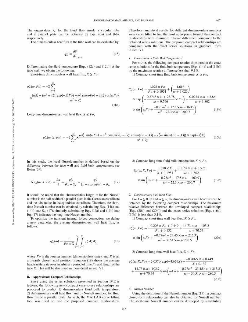
The eigenvalues λn for the fluid flow inside a circular tubeand a parallel plate can be obtained by Eqs. (6a) and (6b),respectively.The dimensionless heat flux at the tube wall can be evaluated by

q�w � ∂θ∂η

��η�1

(15)

Differentiating the fluid temperature [Eqs. (12a) and (12b)] at thetube wall, we obtain the following:Short-time dimensionless wall heat flux, X ≥ Fo,

q�w�ω;Fo� �−2X∞n�1

×�ωλ2n − �ω2 � λ4n��exp�−λ2nFo�−ω2 sin�ωFo�−ωλ2n cos�ωFo�

ω2 � λ4n(16a)

Long-time dimensionless wall heat flux, X ≤ Fo,

q�w�ω; X; Fo� � −2X∞n�1

×ωλ2n sin�ωFo� − ω2 cos�ωFo� − fλ4n cos�ω�Fo − X�� λ2nω sin�ω�Fo − X��g × exp�−λ2nX�

ω2 � λ4n(16b)

In this study, the local Nusselt number is defined based on thedifference between the tube wall and fluid bulk temperatures; seeBejan [39]:

Nua�ω; X; Fo� � ha

k� q�w

θw − θm� q�w

�1� sin�ωFo�� − θm(17)

It should be noted that the characteristics length α for the Nusseltnumber is the half-width of a parallel plate in the Cartesian coordinateand the tube radius in the cylindrical coordinate. Therefore, the short-time Nusselt number can be obtained by substituting Eqs. (14a) and(14b) into Eq. (17); similarly, substituting Eqs. (16a) and (16b) intoEq. (17) indicates the long-time Nusselt number.To optimize the transient internal forced convection, we define

a new parameter, the average dimensionless wall heat flux, asfollows:

�q�w�ω� � 1

Fo × X

ZFo

ξ�0

ZX

ζ�0

q�w dζ dξ (18)

where Fo is the Fourier number (dimensionless time), and X is anarbitrarily chosen axial position. Equation (18) shows the averageheat transfer rate over an arbitrary period of timeFo and length of thetube X. This will be discussed in more detail in Sec. VI.

B. Approximate Compact Relationships

Since using the series solutions presented in Section IV.E istedious, the following new compact easy-to-use relationships areproposed to predict 1) dimensionless fluid bulk temperature;2) dimensionless wall heat flux; and 3) Nusselt number, for fluidflow inside a parallel plate. As such, the MATLAB curve fittingtool was used to find the proposed compact relationships.

Therefore, analytical results for different dimensionless numberswere curve fitted to find the most appropriate form of the compactrelationships with minimum relative difference compared to theobtained series solutions. The proposed compact relationships arecompared with the exact series solutions in graphical formin Sec. VI.

1. Dimensionless Fluid Bulk Temperature

For ω ≥ π, the following compact relationships predict the exactseries solutions for the fluid bulk temperature [Eqs. (14a) and (14b)]by the maximum relative difference less than 9.1%.1) Compact short-time fluid bulk temperature, X ≥ Fo,

θm�ω; Fo� � 1.078 × Fo

Fo� 0.1951��

1.616

ω� 1.023

�

× exp

�−0.3748 × ω� 28.78

ω� 9.796× Fo

�� 0.0934 × ω� 2.86

ω� 1.802

× sin

�ωFo� −0.78ω2 � 17.8 × ω − 160.9

ω2 − 22.3 × ω� 200.7

�(19a)

2) Compact long-time fluid bulk temperature, X ≤ Fo,

θm�ω; X; Fo� � 1.078 × X

X� 0.1951� 0.1167 × ω� 3.575

ω� 1.802

× sin

�ωFo� −0.78ω2 � 17.8 × ω − 160.9

ω2 − 22.3 × ω� 200.7

�(19b)

2. Dimensionless Wall Heat Flux

ForFo ≥ 0.05 andω ≥ π, the dimensionless wall heat flux can beobtained by the following compact relationships. The maximumrelative difference between the developed compact relationships[Eqs. (20a) and (20b)] and the exact series solutions [Eqs. (16a),(16b)] is less than 5.1%.1) Compact short-time wall heat flux, X ≥ Fo,

q�w�ω; Fo� � −0.206 × Fo� 0.449

Fo� 0.132� 14.73 × ω� 103.2

ω� 70.74

× sin

�ωFo� −0.77ω2 − 23.45 × ω� 215.3

ω2 − 30.51 × ω� 280.5

�(20a)

2) Compact long-time wall heat flux, X ≤ Fo,

q�w�ω;X;Fo�� 3.037×exp�−4.626X��−0.206×X�0.449

X�0.132

�14.73×ω�103.2

ω�70.74× sin

�ωFo�−0.77ω2−23.45×ω�215.3

ω2−30.51×ω�280.5

�

(20b)

3. Nusselt Number

Using the definition of the Nusselt number [Eq. (17)], a compactclosed-form relationship can also be obtained for Nusselt number.The short-time Nusselt number can be developed by substituting


Dow

nloa

ded

by S

IMO

N F

RA

SER

UN

IVER

SITY

on

Nov

embe

r 11,

201

5 | h

ttp://

arc.

aiaa

.org

| D

OI:

10.2

514/

1.T4

261

67

Eqs. (17a) and (20a) into Eq. (17). Similarly, the long-time Nusseltnumber can be obtained by substituting Eqs. (19b) and (20b)into Eq. (17).We believe that the form of the compact relationships presented in

this section reveals the nature of the transient problem herein underconsideration. This will be discussed in detail in Sec. VI.

V. Numerical Study

To verify the presented analytical solution, an independent numer-ical simulation of the planar flow inside a parallel plate is performedusing the commercial software ANSYS®Fluent. User-defined codesare written to apply the harmonic and arbitrary time-dependenttemperatures on the tubewall: Eqs. (10) and (22), respectively.Modelgeometry and boundary conditions are similar to what is shown inFig. 1. Furthermore, the assumptions stated in Sec. II are used in thenumerical analysis; however, the fluid axial conduction is notneglected in the numerical analysis. Grid independency of the resultsis tested for three different grid sizes: 20 × 100 and 40 × 200, as wellas 80 × 400. Finally, 40 × 200 is selected as the final grid size, sincethemaximum difference in the predicted values for the fluid tempera-ture by the two latter grid sizes is less than 1%. The geometrical andthermal properties used in the baseline case for the numericalsimulation are listed in Table 2. The maximum relative differencebetween the analytical results and the numerical data is less than4.9%, which is discussed in detail in Sec. VI.

VI. Results and Discussion

A. Harmonic Prescribed Temperature

Although the methodology developed in Sec. III is presented forCartesian and cylindrical coordinates, only the results for the formerare discussed in this section in a graphical form. The trends for thecylindrical coordinate are similar.Variations of the dimensionless centerline temperature against the

Fo number [Eqs. (12a) and (12b)] for a few axial positions along thetube are shown in Fig. 3 and compared with the numerical dataobtained in Sec. V. Periodic temperature is imposed on the tube wall;Eq. (11). The solid lines in Fig. 3 represent our analytical results, andthe markers show the obtained numerical data. There is an excellentagreement between the analytical results [Eqs. (12a) and (12b)] andthe obtained numerical data, with a maximum relative difference lessthan 4.9%.The following is shown in Fig. 3:1) The present model predicts an abrupt transition between the

short-time and long-time responses. The numerical results, however,indicate a smooth transition. This causes the numerical data to deviateslightly from the analytical results as the long-time response begins.Such transitions are demarcated by dashed lines on the figure.

2) The abrupt transition from short-time to long-time responsesis attributed to the analytical method that Siegel [19] used to solvethe transient energy equation for a step wall temperature. This isdiscussed in detail in [19].3) There is an initial transient period of “pure conduction” during

which all the curves follow along the same line, X ≥ Fo; Eq. (12a).4) When Fo � X, each curve moves away from the common line,

i.e., pure conduction response, and adjusts toward a steady oscillatorybehavior at a long-time response; Eq. (12b). The wall temperaturesincrease for largerX values, as expected; this is due to the increase ofthe fluid energy (bulk temperature) along the axial direction.5) Increasing length-to-diameter ratio increases the axial position

number, which in turn increases the temperature inside the fluid.6) The higher the velocity inside the tube, the higher the Re

number, which in turn decreases the axial position number, X ��2x∕a�∕�Rea · Pr� and leads to lower temperature inside the fluid.

Figure 4 shows the variations of the dimensionless fluidtemperature at different radial positions across the tube versus theFonumber; Eqs. (12a) and (12b). Harmonic and step temperatures areimposed at the tube wall, i.e., θw � 1� sin�πFo� and θw � 1, re-spectively. As such, the short-time and long-time fluid temperaturesat different radial positions at an arbitrarily chosen axial position,X � 1.2, are obtained using Eqs. (12a) and (12b).From Fig. 4, the following conclusions can be drawn:1) As expected at any given axial position, the fluid temperature

oscillates with time in the case of a prescribed harmonic wall tem-perature. For a step surface temperature,ω � 0, the solution does notfluctuate over time.2) At any given axial position, there is an initial transient period,

which can be considered as pure conduction, i.e., the short-timeresponse for X ≥ Fo. However, as pointed out earlier, each axialposition shows steady oscillatory behavior for X ≤ Fo at the long-time response. Therefore, for the arbitrarily chosen axial position ofX � 1.2, the long-time response begins at Fo � 1.2 and shows thesame behavior all-time thereafter.3) For an imposed cyclic wall temperature, the fluid temperature

oscillates around the associated response for the step surface tem-peraturewith the sameangular frequency atwhich the system is excited.4) The shift between the peaks of the temperature profile is marked

at different radial positions. This shows a “thermal lag” (phase shift)of the fluid flow, which increases toward the centerline of the tube.This thermal lag is attributed to the fluid thermal inertia.Figure 5 shows the variations of the dimensionless centerline

temperature at a given axial position of X � 1.2 versus the Fouriernumber and the angular frequency; Eqs. (12a) and (12b).The following can be concluded from Fig. 5:1) At the two limiting cases where 1) ω → 0 and 2) ω → ∞, the

fluid flow response yields that of a step surface temperature(isothermal boundary condition).

Fig. 3 Variations of centerline temperature versus the dimensionlesstime (Fourier number) for different axial positions [Eqs. (12a) and (12b)]and comparison with the obtained numerical data (markers).

Fig. 4 Dimensionless fluid temperature against Fo number for cyclic

and step heat fluxes.


Dow

nloa

ded

by S

IMO

N F

RA

SER

UN

IVER

SITY

on

Nov

embe

r 11,

201

5 | h

ttp://

arc.

aiaa

.org

| D

OI:

10.2

514/

1.T4

261

68

2) When a sinusoidal cyclic wall temperature with high angularfrequency is imposed on the flow, the fluid does not follow the detailsof the imposed temperature behavior. Therefore, for high angularfrequencies, the flow acts as if the imposed temperature is constantat “the average value” associated with zero frequency [Eq. (11)] forthe sinusoidal heat flux in this case, in mathematical termsθω→∞ ≈ θω→0.3) A conventional way to decrease the temperature of the working

fluid inside the heat exchangers is to cool down the surface tem-perature. However, it is shown that changing the surface temperaturefrequency can also dramatically alter the fluid temperature.4) The highest temperature for the centerline temperature occurs

for small values of angular frequency. Considering Eq. (12b), thehighest long-time centerline temperature occurs at

dθη�0

dω� 0 ⇒ ω ≈ π �rad� (21)

At a given axial position, the maximum long-time centerlinetemperature is remarkably higher than that of the short-time response.Figure 6 shows the variations of the dimensionless wall heat flux at

a given arbitrary axial position ofX � 1.2 versus the Fourier numberand the dimensionless angular frequency; Eqs. (16a) and (16b). Inaddition, a comparison is made between the exact series solutions[Eqs. (16a) and (16b)] and the developed compact relationships[Eqs. (20a) and (20b)]. As seen from Fig. 6, there is an excellentagreement between the exact solution and the compact relationships;the maximum relative difference less than 4.6%.From Fig. 6, one can conclude the following:1) The dimensionless wall heat flux oscillates with the angular

frequency of the imposed wall temperature. This is indicated by thedeveloped compact relationships; Eqs. (20a) and (20b).

2) The dimensionless wall heat flux oscillates around the step wallheat flux response. In other words, as ω → 0, the dimensionless wallheat flux yields the response of the step wall temperature condition.3) Regardless of the angular frequency, at a very initial transient

period, the dimensionless wall heat flux is much higher than that ofthe long-time response.4) The amplitude of the dimensionless wall heat flux increases

with the angular frequency of the imposedwall temperature. It shouldbe noted that increasing the angular frequency does not affect theamplitude of the imposed wall temperature; see Eq. (9). However, asmentioned before, it decreases the amplitude of the fluid temperaturetoward the centerline. Therefore, as the angular frequency of the

Fig. 5 Centerline temperature against: a) Fo number, b) angular frequency, and c) Fo and angular frequency.

Fig. 6 Exact and approximate wall heat fluxes versus Fo number fordifferent angular frequencies.


Dow

nloa

ded

by S

IMO

N F

RA

SER

UN

IVER

SITY

on

Nov

embe

r 11,

201

5 | h

ttp://

arc.

aiaa

.org

| D

OI:

10.2

514/

1.T4

261

69

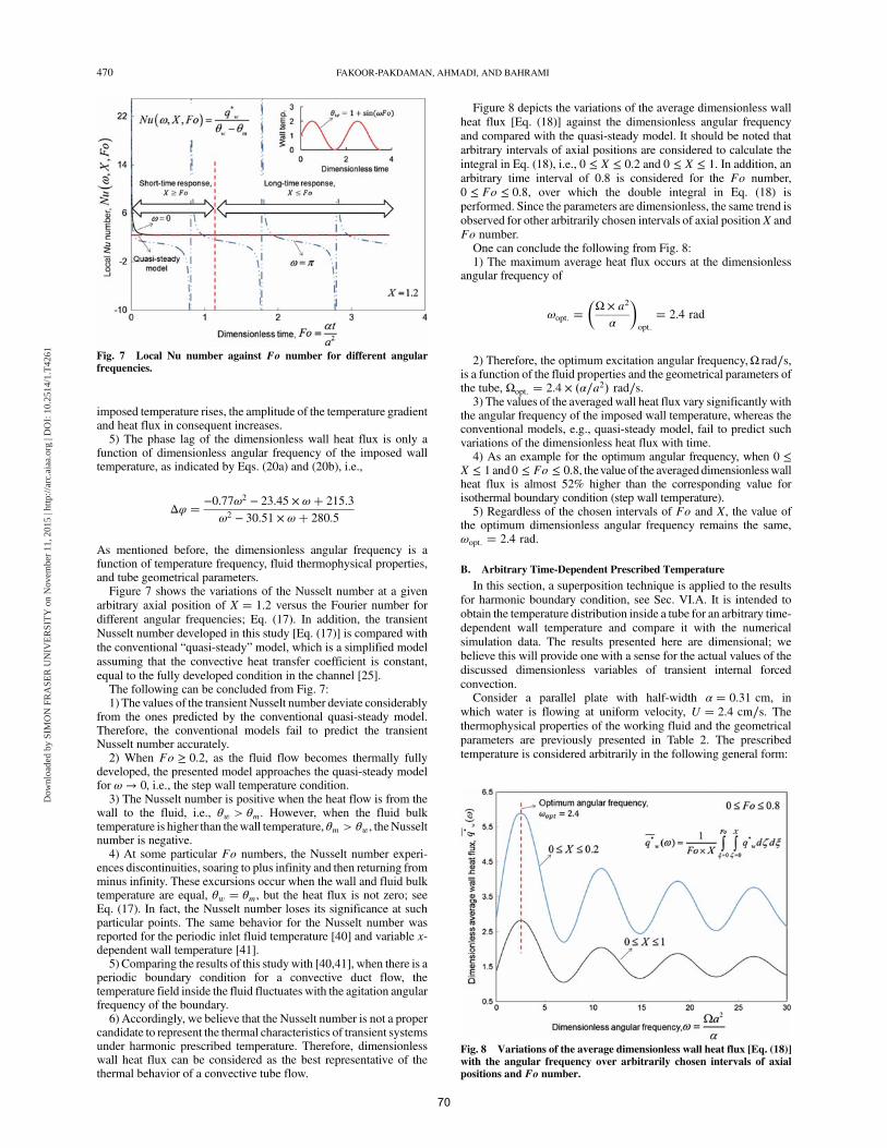
imposed temperature rises, the amplitude of the temperature gradientand heat flux in consequent increases.5) The phase lag of the dimensionless wall heat flux is only a

function of dimensionless angular frequency of the imposed walltemperature, as indicated by Eqs. (20a) and (20b), i.e.,

Δφ � −0.77ω2 − 23.45 × ω� 215.3

ω2 − 30.51 × ω� 280.5

As mentioned before, the dimensionless angular frequency is afunction of temperature frequency, fluid thermophysical properties,and tube geometrical parameters.Figure 7 shows the variations of the Nusselt number at a given

arbitrary axial position of X � 1.2 versus the Fourier number fordifferent angular frequencies; Eq. (17). In addition, the transientNusselt number developed in this study [Eq. (17)] is compared withthe conventional “quasi-steady” model, which is a simplified modelassuming that the convective heat transfer coefficient is constant,equal to the fully developed condition in the channel [25].The following can be concluded from Fig. 7:1) The values of the transient Nusselt number deviate considerably

from the ones predicted by the conventional quasi-steady model.Therefore, the conventional models fail to predict the transientNusselt number accurately.2) When Fo ≥ 0.2, as the fluid flow becomes thermally fully

developed, the presented model approaches the quasi-steady modelfor ω → 0, i.e., the step wall temperature condition.3) The Nusselt number is positive when the heat flow is from the

wall to the fluid, i.e., θw > θm. However, when the fluid bulktemperature is higher than thewall temperature, θm > θw, theNusseltnumber is negative.4) At some particular Fo numbers, the Nusselt number experi-

ences discontinuities, soaring to plus infinity and then returning fromminus infinity. These excursions occur when the wall and fluid bulktemperature are equal, θw � θm, but the heat flux is not zero; seeEq. (17). In fact, the Nusselt number loses its significance at suchparticular points. The same behavior for the Nusselt number wasreported for the periodic inlet fluid temperature [40] and variable x-dependent wall temperature [41].5) Comparing the results of this studywith [40,41], when there is a

periodic boundary condition for a convective duct flow, thetemperature field inside the fluid fluctuates with the agitation angularfrequency of the boundary.6) Accordingly, we believe that the Nusselt number is not a proper

candidate to represent the thermal characteristics of transient systemsunder harmonic prescribed temperature. Therefore, dimensionlesswall heat flux can be considered as the best representative of thethermal behavior of a convective tube flow.

Figure 8 depicts the variations of the average dimensionless wallheat flux [Eq. (18)] against the dimensionless angular frequencyand compared with the quasi-steady model. It should be noted thatarbitrary intervals of axial positions are considered to calculate theintegral in Eq. (18), i.e., 0 ≤ X ≤ 0.2 and 0 ≤ X ≤ 1. In addition, anarbitrary time interval of 0.8 is considered for the Fo number,0 ≤ Fo ≤ 0.8, over which the double integral in Eq. (18) isperformed. Since the parameters are dimensionless, the same trend isobserved for other arbitrarily chosen intervals of axial positionX andFo number.One can conclude the following from Fig. 8:1) The maximum average heat flux occurs at the dimensionless

angular frequency of

ωopt: ��Ω × a2

α

�opt:

� 2.4 rad

2) Therefore, the optimum excitation angular frequency,Ω rad∕s,is a function of the fluid properties and the geometrical parameters ofthe tube, Ωopt: � 2.4 × �α∕a2� rad∕s.

3) The values of the averaged wall heat flux vary significantly withthe angular frequency of the imposed wall temperature, whereas theconventional models, e.g., quasi-steady model, fail to predict suchvariations of the dimensionless heat flux with time.4) As an example for the optimum angular frequency, when 0 ≤

X ≤ 1 and0 ≤ Fo ≤ 0.8, thevalue of the averageddimensionlesswallheat flux is almost 52% higher than the corresponding value forisothermal boundary condition (step wall temperature).5) Regardless of the chosen intervals of Fo and X, the value of

the optimum dimensionless angular frequency remains the same,ωopt: � 2.4 rad.

B. Arbitrary Time-Dependent Prescribed Temperature

In this section, a superposition technique is applied to the resultsfor harmonic boundary condition, see Sec. VI.A. It is intended toobtain the temperature distribution inside a tube for an arbitrary time-dependent wall temperature and compare it with the numericalsimulation data. The results presented here are dimensional; webelieve this will provide one with a sense for the actual values of thediscussed dimensionless variables of transient internal forcedconvection.Consider a parallel plate with half-width α � 0.31 cm, in

which water is flowing at uniform velocity, U � 2.4 cm∕s. Thethermophysical properties of the working fluid and the geometricalparameters are previously presented in Table 2. The prescribedtemperature is considered arbitrarily in the following general form:

Fig. 8 Variations of the average dimensionless wall heat flux [Eq. (18)]with the angular frequency over arbitrarily chosen intervals of axialpositions and Fo number.

Fig. 7 Local Nu number against Fo number for different angularfrequencies.


Dow

nloa

ded

by S

IMO

N F

RA

SER

UN

IVER

SITY

on

Nov

embe

r 11,

201

5 | h

ttp://

arc.

aiaa

.org

| D

OI:

10.2

514/

1.T4

261

70

Tw � T0 �X4i�1

�Ti � ΔTR;i sin�Ωit�� (22)

The parameters in Eq. (22) are introduced in Table 3. It should benoted that T0 is the initial temperature of the fluid, and Ti and ΔTR;i

are the constant values and the amplitudes of the imposed walltemperature, respectively. The values for the parameters in Eq. (22)are arbitrarily chosen, and a similar approach can be taken for otherforms of time-dependent boundary conditions.Figure 9 displays the transient centerline temperature, at an

arbitrarily chosen axial position, x � 50 cm, under a time-dependentwall temperature [Eq. (22)] in comparison with the obtainednumerical data. The imposed wall temperature is also depicted inFig. 9 by a solid line. Themarkers in Fig. 9 are the numerical data, andthe solid lines are the analytical results. There is a good agreementbetween the analytical results and the numerical simulation data; themaximum relative difference is less than 5%.The following can be concluded from Fig. 9:1) The short-time response, t ≤ 21 s, at which pure conduction

heat transfer occurs is much lower than the long time response,t ≥ 21 s.

2) The presentedmodel can be applied to find the fluid temperatureinside a tube under any type of arbitrary time-dependent walltemperature.3) The maximum discrepancy between the analytical results and

the obtained numerical data occurs around the transition time, asstated for the trends in Fig. 3. This occurs since the analytical modelpredicts an abrupt arrival from short-time to long-time response,whereas the numerical simulation predicts a smooth transition; see[19] for more detail.

VII. Conclusions

A new full-time-range analytical model is developed to predict thetransient thermal performance of forced-convective tube flow underan arbitrary time-dependent wall temperature. The methodology ispresented in Cartesian and cylindrical coordinates. The slug flowcondition is considered for the velocity distribution inside a circulartube. As such, new all-time models are developed to evaluate1) temperature distribution inside the fluid; 2) fluid bulk temperature;3) dimensionless wall heat flux; and 4)Nusselt number. Furthermore,compact closed-form relationships are proposed to predict suchthermal characteristics of the tube flow with the maximum relativedifference of less than 10%. A new heat transfer enhancement tech-nique is presented for convective tube flow under harmonic boundarytemperature. Optimizing the angular frequency of the imposed walltemperature can remarkably increase the overall heat transfer rate of aconvective tube flow. The analytical results are verified successfullywith the obtained numerical data. The maximum relative differencebetween the analytical results and the numerical data is less than4.9%. The highlights of the present study can be listed as follows:1) There is a thermal lag in the thermal response of the fluid

temperature that increases toward the centerline of the tube due to thethermal inertia of the fluid.2) The fluid temperature, dimensionlesswall heat flux, andNusselt

number oscillate with the angular frequency of the imposed walltemperature.3)At the two limiting cases, the thermal response of the fluid yields

that of the step wall temperature: 1) ω → 0 and 2) ω → ∞.

Table 2 Fluid properties and dimensionsof the tube for the baseline case in numerical

simulationa

Parameter ValueThermal conductivity k, W∕m∕k 0.64Thermal diffusivity α, m2∕s 1.6E-7Kinematic viscosity ν, m2∕s 5.66E-7Tube half-width a, m 0.003Tube length L, cm 250

aRea � 100.

Table 3 Parametersin Eq. (22)

Parameter Value

T0, K 300Ω1, rad∕s 0.06Ω2, rad∕s 0.12Ω3, rad∕s 0.24Ω4, rad∕s 0.1ΔTR;1, K 1ΔTR;2, K 4ΔTR;3, K 10ΔTR;4, K 8T1, K 5T2, K 10T3, K 15T4, K 20

Fig. 9 Centerline temperature [Eq. (11)] versus time, and comparisonwith the obtained numerical data for a general boundary condition[Eq. (20)].

Table 1 Summary of the literature regarding unsteady internal forced convection

Author Velocity profile Notes

Siegel [19] Slug flow Reported temperature distribution inside the fluid in Cartesian and cylindrical coordinates.Limited to step wall temperature/heat flux.

Siegel [20] Poiseuille flow Reported temperature distribution inside the fluid in cylindrical coordinate.Limited to step wall temperature condition.

Sparrow and Siegel [21,22] Poiseuille flow Reported tube wall temperature/heat flux.Limited to homogenous boundary conditions, i.e., step wall temperature/heat flux.Limited to thermal entrance region.

Perlmutter and Siegel [26] Poiseuille flow Evaluated tube wall temperature considering the wall thermal inertia.Limited to step wall temperature condition.

Sucec [27] Slug flow Evaluated fluid temperature under sinusoidal wall heat flux.Limited to quasi-steady assumption.


Dow

nloa

ded

by S

IMO

N F

RA

SER

UN

IVER

SITY

on

Nov

embe

r 11,

201

5 | h

ttp://

arc.

aiaa

.org

| D

OI:

10.2

514/

1.T4

261

71

4) There is an optimum value for the dimensionless angularfrequency of the imposed harmonic wall temperature that maximizesthe average dimensionless wall heat flux:

ωopt: ��Ω × a2

α

�opt:

� 2.43 rad

Acknowledgments

This work was supported by Automotive Partnership Canada,grant no. APCPJ 401826-10. The authors would like to thank thesupport of the industry partner Future Vehicle Technologies, Inc.(British Columbia, Canada).

References

[1] Agyenim, F., Hewitt, N., Eames, P., and Smyth, M., “A Review ofMaterials, Heat Transfer and Phase Change Problem Formulation forLatent Heat Thermal Energy Storage Systems (Lhtess),”Renewable andSustainable Energy Reviews, Vol. 14, No. 2, Feb. 2010, pp. 615–628.doi:10.1016/j.rser.2009.10.015

[2] Cabeza, L. F., Mehling, H., Hiebler, S., and Ziegler, F., “Heat TransferEnhancement inWater whenUsed as PCM in Thermal Energy Storage,”Applied Thermal Engineering, Vol. 22, No. 10, July 2002, pp. 1141–1151.doi:10.1016/S1359-4311(02)00035-2

[3] Kurklo, A., “Energy Storage Applications in Greenhouses by Meansof Phase Change Materials (PCMs): A Review,” Renewable Energy,Vol. 13, No. 1, 1998, pp. 89–103.doi:10.1016/S0960-1481(97)83337-X

[4] Garrison, J. B., and Webber, E. M., “Optimization of an IntegratedEnergy Storage for a Dispatchable Wind Powered Energy System,”ASME 2012 6th International Conference on Energy Sustainability,American Soc. of Mechanical Engineers, Fairfield, NJ, 2012, pp. 1–11.

[5] Sawin, J. L., and Martinot, E., “Renewables Bounced Back in 2010,Finds REN21 Global Report,” Renewable Energy World, 2011, Dataavailable online at http://www.renewableenergyworld.com/rea/news/article/2011/09/renewables-bounced-back-in-2010-finds-ren21-global-report [retrieved 2014].

[6] Bennion, K., and Thornton, M., “Integrated Vehicle ThermalManagement for AdvancedVehicle Propulsion Technologies,”NationalRenewable Energy Lab. NREL/CP-540-47416, Golden, CO, 2010.

[7] Boglietti, A., Member, S., Cavagnino, A., Staton, D., Shanel, M.,Mueller, M., and Mejuto, C., “Evolution and Modern Approaches forThermal Analysis of Electrical Machines,” IEEE Transactions on

Industrial Electronics, Vol. 56, No. 3, 2009, pp. 871–882.doi:10.1109/TIE.2008.2011622

[8] Canders, W.-R., Tareilus, G., Koch, I., and May, H., “New Design andControl Aspects for Electric Vehicle Drives,” 2010 14th International

Power Electronics and Motion Control Conference (EPE/PEMC),IEEE Xplore, Sept. 2010, pp. S11-1, S11-8.doi:10.1109/EPEPEMC.2010.5606528

[9] Hamada, K., “Present Status and Future Prospects for Electronics inElectric Vehicles/Hybrid Electric Vehicles and Expectations for WideBandgap Semiconductor Devices,” Physica Status Solidi (B), Vol. 245,No. 7, July 2008, pp. 1223–1231.doi:10.1002/pssb.v245:7

[10] Hale, M., “Survey of Thermal Storage for Parabolic Trough PowerPlants,” National Renewable Energy Lab. NREL/SR-550-27925,Golden, CO, 2000, pp. 1–28.

[11] Sharma, A., Tyagi, V. V., Chen, C. R., and Buddhi, D., “Review onThermal Energy Storage with Phase Change Materials and Applica-tions,” Renewable and Sustainable Energy Reviews, Vol. 13, No. 2,Feb. 2009, pp. 318–345.doi:10.1016/j.rser.2007.10.005

[12] März, M., Schletz, A., Eckardt, B., Egelkraut, S., and Rauh, H., “PowerElectronics System Integration for Electric and Hybrid Vehicles,”Integrated Power Electronics Systems (CIPS), IEEE Xplore,March 2010, pp. 1–10, 16–18, Data available online at http://ieeexplore.ieee.org/stamp/stamp.jsp?tp=&=5730643&=5730626.

[13] Nerg, J., Rilla, M., and Pyrhönen, J., “Thermal Analysis of Radial-FluxElectricalMachines with a High Power Density,” IEEE Transactions on

Industrial Electronics, Vol. 55, No. 10, 2008, pp. 3543–3554.doi:10.1109/TIE.2008.927403

[14] “Cumulative Sales of TMC Hybrids Top 2 Million Units in Japan,”Toyota Motor Corporation, Japan, 2012, Data available online at

http://www.toyotabharat.com/inen/news/2013/april_17.aspx [retrieved2014].

[15] O’Keefe, M., and Bennion, K., “A Comparison of Hybrid ElectricVehicle Power Electronics Cooling Options,” IEEE Vehicle Power and

PropulsionConference (VPPC), IEEEXplore, 2007, pp. 116–123, 9–12.doi:10.1109/VPPC.2007.4544110

[16] Bennion, K., and Thornton, M., “Integrated Vehicle Thermal Mana-gement for Advanced Vehicle Propulsion Technologies,” NationalRenewable Energy Lab. NREL/CP-540-47416, Golden, CO, 2010.

[17] Johnson, R. W., Evans, J. L., Jacobsen, P., Thompson, J. R. R., andChristopher, M., “The Changing Automotive Environment: High-Temperature Electronics,” IEEE Transactions on Electronics Packag-

ing Manufacturing, Vol. 27, No. 3, July 2004, pp. 164–176.doi:10.1109/TEPM.2004.843109

[18] Kelly, K., Abraham, T., and Bennion, K., “Assessment of ThermalControl Technologies for Cooling Electric Vehicle Power Electronics,”National Renewable Energy Lab. NREL/CP-540-42267, Golden, CO,2008.

[19] Siegel, R., “Transient Heat Transfer for Laminar Slug Flow in Ducts,”Applied Mechanics, Vol. 81, No. 1, 1959, pp. 140–144.

[20] Siegel, R., “Heat Transfer for Laminar Flow in Ducts with ArbitraryTime Variations in Wall Temperature,” Journal of Applied Mechanics,Vol. 27, No. 2, 1960, pp. 241–249.doi:10.1115/1.3643945

[21] Sparrow, E. M., and Siegel, R., “Thermal Entrance Region of a CircularTube Under Transient Heating Conditions,” Third U.S. National

Congress of Applied Mechanics, ASME Trans., 1958, pp. 817–826.[22] Siegel, R., and Sparrow, E. M., “Transient Heat Transfer for Laminar

Forced Convection in the Thermal Entrance Region of Flat Ducts,”ASME Heat Transfer, Vol. 81, No. 1, 1959, pp. 29–36.

[23] Perlmutter, M., and Siegel, R., “Unsteady Laminar Flow in a Ductwith Unsteady Heat Addition,” Heat Transfer, Vol. 83, No. 4, 1961,pp. 432–439.doi:10.1115/1.3683662

[24] Siegel, R., “Forced Convection in a Channel with Wall Heat Capacityand with Wall Heating Variable with Axial Position and Time,”International Journal of Heat Mass Transfer, Vol. 6, No. 7, 1963,pp. 607–620.doi:10.1016/0017-9310(63)90016-4

[25] Siegel, R., and Perlmutter, M., “Laminar Heat Transfer in a ChannelwithUnsteady Flow andWall HeatingVaryingwith Position and Time,”Journal of Heat Transfer, Vol. 85, No. 4, 1963, pp. 358–365.doi:10.1115/1.3686125

[26] Perlmutter, M., and Siegel, R., “Two-Dimensional Unsteady Incom-pressible Laminar Duct Flowwith a Step Change inWall Temperature,”Journal of Heat Transfer, Vol. 83, No. 4, 1961, pp. 432–440.doi:10.1115/1.3683662

[27] Sucec, J., “Unsteady Forced Convection with Sinusoidal Duct WallGeneration: The Conjugate Heat Transfer Problem,” International

Journal of Heat and Mass Transfer, Vol. 45, No. 8, April 2002,pp. 1631–1642.doi:10.1016/S0017-9310(01)00275-7

[28] Kakac, S., Li, W., and Cotta, R. M., “Unsteady Laminar ForcedConvection inDuctswith PeriodicVariation of Inlet Temperature,”HeatTransfer, Vol. 112, No. 4, 1990, pp. 913–920.doi:10.1115/1.2910499

[29] Weigong, L., and Kakac, S., “Unsteady Thermal Entrance Heat Transferin Laminar Flow with a Periodic Variation of Inlet Temperature,”International Journal of Heat and Mass Transfer, Vol. 34, No. 10,Oct. 1991, pp. 2581–2592.doi:10.1016/0017-9310(91)90098-Y

[30] Kakac, S., and Yener, Y., “Exact Solution of the Transient ForcedConvection Energy Equation for Timewise Variation of Inlet Temper-ature,” International Journal of Heat Mass Transfer, Vol. 16, No. 12,1973, pp. 2205–2214.doi:10.1016/0017-9310(73)90007-0

[31] Cotta, R. M., and Özişik, M. N., “Laminar Forced Convection InsideDucts with Periodic Variation of Inlet Temperature,” International

Journal of Heat andMass Transfer, Vol. 29, Oct. 1986, pp. 1495–1501.doi:10.1016/0017-9310(86)90064-5

[32] Kakac, S., “AGeneral Analytical Solution to the Equation of TransientForced Convection with Fully Developed Flow,” International Journalof Heat Mass Transfer, Vol. 18, No. 12, 1975, pp. 1449–1454.doi:10.1016/0017-9310(75)90259-8

[33] Hadiouche, A., and Mansouri, K., “Application of Integral TransformTechnique to the Transient Laminar Flow Heat Transfer in the Ducts,”International Journal of Thermal Sciences, Vol. 49, No. 1, Jan. 2010,pp. 10–22.doi:10.1016/j.ijthermalsci.2009.05.012


Dow

nloa

ded

by S

IMO

N F

RA

SER

UN

IVER

SITY

on

Nov

embe

r 11,

201

5 | h

ttp://

arc.

aiaa

.org

| D

OI:

10.2

514/

1.T4

261

72

[34] Fakoor-Pakdaman, M., Andisheh-Tadbir, M., and Bahrami, M.,“Transient Internal Forced Convection Under Arbitrary Time-Dependent Heat Flux,” Proceedings of the ASME 2013 Summer Heat

Transfer Conference HT2013, ASME-17148,Minneapolis, MN, 2013.[35] Fakoor-Pakdaman, M., Andisheh-Tadbir, M., and Bahrami, M.,

“Unsteady Laminar Forced-Convective Tube Flow Under DynamicTime-Dependent Heat Flux,” Journal of Heat Transfer, Vol. 136, No. 4,Nov. 2013, Paper 041706.doi:10.1115/1.4026119

[36] Kreyszig, E., Kreyzig, H., and Norminton, E. J., Advanced EngineeringMethematics, Wiley, New York, 2010, pp. 473–490.

[37] Campo, A., Morrone, B., and Manca, O., “Approximate AnalyticEstimate of Axial Fluid Conduction in Laminar Forced Convection

Tube Flows with Zero-to-Uniform Step Wall Heat Fluxes,” Heat

Transfer Engineering, Vol. 24, No. 4, July 2003, pp. 49–58.doi:10.1080/01457630304027

[38] Incropera, F. P., Dewitt, D. P., Bergman, T. L., and Lavine, A. S.,Introduction to Heat Transfer, Wiley, New York, 2007, p. 458.

[39] Bejan, A., Convection Heat Transfer, Wiley, New York, 2004, p. 119.[40] Sparrow, E. M., and Farias, F. N. De., “Unsteady Heat Transfer in Ducts

With Time-Varying Inlet Tempearture and Participating Walls,”International Journal of Heat Mass Transfer, Vol. 11, No. 5, 1968,pp. 837–853.doi:10.1016/0017-9310(68)90128-2

[41] Kays,W.M., andCrawford,M. E.,ConvectiveHeat andMass Transfer,McGraw–Hill, New York, 1993, pp. 140–146.


Dow

nloa

ded

by S

IMO

N F

RA

SER

UN

IVER

SITY

on

Nov

embe

r 11,

201

5 | h

ttp://

arc.

aiaa

.org

| D

OI:

10.2

514/

1.T4

261

73

Appendix B

Optimal unsteady convection over a duty cycle for arbitrary unsteady flow under dynamic thermal load

74

Optimal unsteady convection over a duty cycle for arbitrary unsteadyflow under dynamic thermal load

M. Fakoor-Pakdaman ⇑, Mehran Ahmadi, Mehdi Andisheh-Tadbir, Majid BahramiLaboratory for Alternative Energy Conversion (LAEC), School of Mechatronic Systems Engineering, Simon Fraser University, Surrey, BC, Canada

a r t i c l e i n f o

Article history:Received 30 April 2014Received in revised form 18 July 2014Accepted 20 July 2014Available online 15 August 2014

Keywords:ConvectionDynamic systemsPulsating flowTransientOptimal frequencyAPEEM

a b s t r a c t

Developing next generation transient heat exchangers is a transformative technology for efficient ther-mal management of advanced power electronics and electric machines (APEEM) inside hybrid electric,electric, and fuel cell vehicles as well as renewable energies (wind, solar, tidal). Optimal design criteriafor such dynamic heat exchangers should be achieved through addressing internal forced convectionwith arbitrary flow unsteadiness under dynamic time dependent thermal loads. Exact analytical solutionswere obtained for laminar forced-convective heat transfer under arbitrary time-dependent heat flux forsteady flow inside a tube (Fakoor-Pakdaman et al., 2014). In this study, the energy equation is solved ana-lytically for arbitrary unsteady flow between parallel plates under dynamic time and position dependentheat flux. As such, laminar pulsating flow between two parallel plates is considered under a harmonicwall heat flux. Exact relationships are obtained to find; (i) temperature distribution for the fluid; (ii) fluidbulk temperature; and (iii) the local and time averaged Nusselt number. New compact relationships areproposed to find the thermal entrance length and the cyclic fully-developed Nusselt number. It is shownthat the period of the Nusselt number oscillations is the least common multiple of the periods of theimposed harmonic heat flux and the pulsating flow. We obtained a relationship for the ‘cut-off’ angularfrequency of pulsating flow beyond which the heat transfer does not feel the pulsation. This study alsoshows that for a given harmonic wall heat flux, there is an optimal pulsating flow velocity, with optimumfrequency, which enhances the time averaged Nusselt number by up to 27%.

� 2014 Elsevier Ltd. All rights reserved.

1. Introduction

Optimal design of transient single-phase heat exchangers is akey to developing innovative technology for the next generationadvanced power electronics and electric machines (APEEM).APEEM has applications in emerging cleantech systems such aspowertrain and propulsion systems of hybrid electric, electric vehi-cles (EV), and emerging fuel cell vehicles (FCV) [1,2] and greenpower systems (wind, solar, tidal) [3,4]. Heat generation in APEEMundergo substantial transitions as a direct result of; (i) variableload due to duty cycle, [5–8] and (ii) unsteady coolant flow rateover a duty cycle [9,10]. As such, the heat exchangers/heat sinksassociated with APEEM operate periodically over time and neverattain a steady-state condition. Conventionally, cooling systemsare designed based on a nominal steady-state or a ‘‘worst’’ casescenario, which may not properly represent the thermal behavior

of various applications or duty cycles [7]. Downing and Kojasoy[11] predicted heat fluxes of 150 � 200 [W/cm2] and pulsedtransient heat loads up to 400 [W/cm2], for the next-generationinsulated gate bipolar transistors (IGBTs) which are used in thedesign of inverter units of HEVs.

Processes such as start-up, shut down, and pump/fan failure areother typical examples of arbitrary flow unsteadiness for dynamic/transient heat exchangers [12–15]. Besides, depending on the func-tionality of APEEM over a duty cycle, the coolant flow rate insidethe heat exchangers/heat sinks of HE/E/FCV is varying arbitrarilyover time [16]. Conventionally mechanical water pumps, directlycoupled to the engine, are used in gasoline/diesel vehicles. How-ever, electric vehicles can use variable-speed electric water pumpusing a separate electric motor and a controller, therefore main-taining an ‘optimal’ and variable flow rate of the coolant is possibleover a driving cycle [9,10]. This provides an opportunity to signif-icantly reduce the parasitic power required for the cooling of HE/E/FCV APEEM and improve the overall efficiency of the vehicle. Thereare only a few studies in the open literature on this topic. There-fore, there is a pending need for an in-depth understanding ofinstantaneous thermal characteristics of transient cooling systems

http://dx.doi.org/10.1016/j.ijheatmasstransfer.2014.07.0580017-9310/� 2014 Elsevier Ltd. All rights reserved.

⇑ Corresponding author. Tel.: +1 (778) 782 8538; fax: +1 (778) 782 7514.E-mail addresses: [email protected] (M. Fakoor-Pakdaman), [email protected]

(M. Ahmadi), [email protected] (M. Andisheh-Tadbir), [email protected](M. Bahrami).

International Journal of Heat and Mass Transfer 78 (2014) 1187–1198

Contents lists available at ScienceDirect

International Journal of Heat and Mass Transfer

journal homepage: www.elsevier .com/locate / i jhmt

75

over a given duty cycle. This study is focused on internal forcedconvection with arbitrary unsteadiness in flow under arbitrarytime-varying heat flux. The results of this work will provide a plat-form for the design, validation and building new intelligent ther-mal management systems that can actively and proactivelycontrol variable-speed electric pumps to circulate a coolant withinstantaneous optimal flow rate in APEEM and similar applications.

1.1. Present literature

Siegel [17] pioneered the study on transient internal forced-convective heat transfer. He conducted several studies to investi-gate the thermal characteristics of steady tube flow under step wallheat flux/temperature [18–20]. Laminar pulsating flow is alsoaddressed in Siegel’s study [21] for planar flow in parallel platesunder constant heat flux/wall temperature cases. It is shown thatquasi-steady assumption does not give an accurate prediction ofthe thermal characteristics of the pulsating flow for moderaterange of pulsation frequency [21]. Guo and Sung [22] addressedthe contradictory results of the Nusselt number for pulsating flowin previous published papers; as some researchers had reportedheat transfer enhancement, see Refs. [23,24], while heat transferreduction had been noted in Ref. [25]. They proposed a new modelfor the time-averaged Nusselt number of laminar pulsating flowunder constant wall heat flux. Such definition was introducedbased on the time-averaged differences between the tube-walland fluid-bulk temperatures over a pulsation period. Hemidaet al. [26] argued that the small effects of pulsation, which hadbeen noted in previous studies occurred as a result of the restric-tive boundary conditions. Wall temperature/heat flux wasassumed constant both in space and time. This may affect the heatexchange process, and reduce the effects of pulsation. This showsthe necessity to consider more realistic boundary conditions forthe tube wall other than constant heat flux or temperature.Less restrictive boundary conditions might manifest into greater

sensitivity to pulsation [26]. This is one of the key issues addressedin the present study. In addition, Brereten and Jiang [27]introduced the idea of fluid flow modulation to increase thetime-averaged Nusselt number of pulsating flow under constantheat flux. A summary of literature on laminar pulsating flow ispresented in Table 1. Our literature review indicates:

� The existing models for pulsating channel flow are limited toconstant wall heat flux/temperature cases.

� Effects of simultaneous oscillation of imposed heat flux andfluid velocity are not investigated in the literature.

� There is no model to determine an optimal velocity frequencyfor a given harmonic heat flux to maximize the convective heattransfer rate.

To the best of our knowledge, effects of non-constant boundaryconditions have not been investigated in the literature neitherexperimentally nor theoretically. In other words, the answer tothe following question is not clear: ‘‘can flow pulsation enhancethe heat transfer rate in heat exchangers under arbitrary time-dependent loads?’’

In our previous studies [31,32], a comprehensive analyticalstudy was performed to predict the thermal characteristics of lam-inar steady flow under dynamic time-dependent wall heat flux. Inthe present study, a new analytical model is developed for laminar,single-phase heat transfer between two parallel plates with arbi-trary flow unsteadiness under arbitrary time/position dependentwall heat flux. Laminar pulsating flow and harmonic heat flux areconsidered to obtain exact relationships for: (i) fluid temperaturedistribution inside the channel; (ii) fluid bulk temperature; and(iii) the Nusselt number. The period of Nusselt number oscillationis obtained under simultaneous oscillation of flow and the imposedwall heat flux. Following Ref. [23], a new definition is introduced toobtain the time-averaged Nusselt number. In addition, optimal pul-sating velocity with optimum frequency is found that maximizes

Nomenclature

a Half width of the parallel plates, [m]cp heat capacity, [J/kg K]f Arbitrary function of time, Eq. (2), ¼ uðtÞ

ur

Fn Eigen values, Eq. (7)Fo Fourier number, = at/R2

h Local heat transfer coefficient, Eq. (23), [W/m2 K]k Thermal conductivity, (W/m K)n Positive integer, Eq. (7), = 1,2,3,. . .Nua Local Nusselt number, Eq. (23), = ha/kp Dimemsionless period of temperature fluctuationp1 Dimensionless period of heat flux fluctuation, ¼ 2p

x1

p2 Dimensionless period of pulsatile velocity, ¼ 2px2

Pe Peclet number, = Re � PrPr Prandtl number, = m/aq00 Thermal load (Heat flux), [W/m2]Re Reynolds number, = 4ura/tt Time, [s]T Temperature, [K]u Velocity, [m/s]x Axial distance from the entrance of the heated section,

[m]y Normal coordinate measured from centerline of parallel

plate channel, [m]X Dimensionless axial coordinate, = 4x/Re � Pr � aY Dimensionless normal coordinate, = y/a

Greek lettersa Thermal diffusivity, [m2/s]m Kinematic viscosity, [m2/s]q Fluid density, [kg/m3]h Dimensionless temperature, ¼ T�T0

q00r a=k

u Arbitrary function of X and Fo, Eq. (4)X1 Angular frequency of the heat flux, [rad/s]X2 Angular frequency of the fluid velocity, [rad/s]x1 Dimensionless angular frequency of the wall heat

flux, =X1a2/a

x2 Dimensionless angular frequency of the fluid veloc-ity, =X2a

2/as Dimensionless arbitrary timen Dummy Fo variablef Dummy X variable

Subscripts0 Inletm Mean or bulk valuew wallr Reference values Step heat fluxTr. Transition

1188 M. Fakoor-Pakdaman et al. / International Journal of Heat and Mass Transfer 78 (2014) 1187–1198

76

the heat transfer rate in the channel flow under a given harmonicwall heat flux. An independent numerical study is also performedwhich compares well with the analytical results;maximum relativedifference less than 6%.

To develop the present analytical model, the fluid flow responseto a step heat flux is taken into account. A Duhamel’s theorem isapplied on the thermal response of the fluid flow under the stepheat flux, following Ref. [17]. The methodology presented in Ref.[32] is extended to account for arbitrary flow unsteadiness underarbitrary wall heat flux. A harmonic heat flux and pulsatinglaminar flow are taken into consideration and the thermal charac-teristics of the fluid flow are determined analytically. Since anytime-dependent wall heat flux can be expressed by simpleoscillatory functions using a Fourier series transformation [33],the results of this study can be readily applied to determine thepulsating fluid flow response under an arbitrary time-varying heatflux. This approach enables analyzing transient single-phaseconvective heat transfer under various time-varying conditions,using a superposition technique.

2. Governing equations

Fig. 1 shows fluid flow between two parallel plates with halfwidth of spacing, a, which is thermally insulated in the firstsub-region, x 6 0, and is heated in the second sub-region, x > 0.The entering fluid temperature is maintained at T0 throughout

the heating period. The wall at the second sub-region is given byan arbitrary time-dependent heat flux, q00(t). It should be noted thatthe second sub-region may be long enough so that the flow canreach thermally fully-developed condition, see Fig. 1. It is intendedto determine the evolution of the channel wall temperature, fluidbulk temperature and the Nusselt number as a function of timeand space for the entire range of time. Such characteristics areevaluated under dynamic time-dependent heat flux for a fluid flowwith arbitrary time-varying velocity.

The assumptions made in deriving the proposed analyticalmodel are listed below:

� Incompressible flow,� Constant thermo-physical properties,� Negligible viscous dissipation,� Negligible axial heat conduction, i.e., Pe = Re � PrP 10 [25],� No thermal energy sources within the fluid,� No flow reversal in the duct,� Fluid flow velocity is only a function of time, i.e., slug flowu = u(t).

The slug flow approximation means consideration of one-dimensional velocity distribution, i.e., the fluid is moving throughthe channel with a mean velocity that can be a function of time.As demonstrated in Refs. [17,20], the slug flow approximationreveals the essential physical behavior of the system, while itenables obtaining exact mathematical solution for various bound-ary conditions. Using this simplification one can study the effectsof various boundary conditions on transient heat transfer withouttedious numerical computations [17,20].

The energy equation for a slug flow inside two parallel plates isthen become:

@T@t

þ uðtÞ @T@x

¼ a@2T@y2

!ð1Þ

where the transient velocity between the parallel plates, u(t), in theenergy equation can be written as follows:

uðtÞ ¼ ur � f ðtÞ ð2Þ

Here ur is a constant reference velocity, and f(t) is an arbitrary func-tion of time. For a special case where f(t) = 1, the channel flow veloc-ity is constant slug flow, u = ur, which was investigated in our

Table 1Summary of the literature on laminar pulsating channel flow.

Author Approach Notes

Siegel and Perlmutter[21]

Analytical (method of characteristics)p

Reported temperature distribution between two parallel platespCovered thermally developing and fully-developed regions

� Limited to step wall temperature and heat flux� Nusselt number was defined based on the tube wall and inlet fluid temperature

Hemida et al. [26] Analytical/numerical (Green’s functionsolution)

pReported a closed-form relationship for the temperature distribution in fully-developedregionpConsidered different BCs: (i) isoflux; (ii) wall with thermal resistance; (iii) wall with ther-mal inertia

� Treated thermally developing region only numericallyNield and Kuznetsov

[28]Analytical (perturbation method)

pReported transient Nusselt number in circular tubes and parallel platespDefinition of the Nusselt number similar to [22]

� Reported singularity in the solution for Pr = 1� Limited to constant wall heat flux� Limited to oscillations with small amplitudes

Zhao and Cheng [29] Numericalp

Proposed a compact relationship for the time averaged Nusselt number for reciprocatingflowpCovered both thermally developing and fully-developed regions

� Limited to constant wall temperatureYan et al. [30] Analytical/experimental

pReported series solutions for temperature distribution and Nusselt number

� Limited to constant wall temperature

Thermallyfully-developed

region

Insulated section, Heated section,

Inlettemp.,

Heatflux,

Time [s]

Thermalentrance

region Fluid vel.,

Fig. 1. Schematic of the developing and fully-developed regions, time-dependentwall heat flux and fluid velocity as well as the coordinate system.

M. Fakoor-Pakdaman et al. / International Journal of Heat and Mass Transfer 78 (2014) 1187–1198 1189

77

previous works [31,32]. As such, the dimensionless form of theenergy equation, Eq. (1), then becomes:

@h@Fo

þ uur

@h@X

¼ @2h

@Y2 ð3Þ

We define the following dimensionless variables:

Fo ¼ ata2

X ¼ 4x=aRe � Pr h ¼ T � T0

q00r a=k

Y ¼ ya

Re ¼ 4urat

Pr ¼ ta

where Fo is the Fourier number and X is the dimensionless axiallocation that characterizes the flow inside a conduit. As previouslymentioned, the goal of this study is to find the transient thermalresponse of unsteady forced-convective channel flow under arbi-trary time-dependent wall heat flux. Therefore, a general wall heatflux is assumed as:

q00ðX; FoÞ ¼ q00r � u X; Foð Þ ð4Þ

where q00r is the heat flux amplitude and u (X,Fo) is an arbitrary

function of space and time, respectively. Consequently, Eq. (4) issubjected to the following initial and boundary conditions:

h Y;X;0ð Þ ¼ 0 Initial condition;h Y; 0; Foð Þ ¼ 0 Entrance condition;

@h=@Yð ÞjY¼1 ¼ q00

q00rX; Foð Þ ¼ uðX; FoÞ

Heat flux at the channel wall for Fo > 0;@h=@Yð ÞjY¼0 ¼ 0 Symmetry at the channel centerline: ð5ÞAlthough the analysis here are performed for fluid flow betweenparallel plates, the same methodology can be adopted for othergeometries, see Ref. [34] for more detail.

3. Model development

In this section, a new all-time model is developed considering;(i) short-time response and (ii) long-time response. When a slab atuniform temperature T0 is suddenly subjected to a step heat flux Dq00 at its surface, the temperature response is [17]:

hs ¼ T � T0

q00r a=k

¼ Dq00

q00r

Foþ 3Y2 � 16

� 2X1n¼1

�1ð ÞnF2n

� cos FnYð Þ � exp �F2n � Fo

� �" #

ð6Þwhere hs is the dimensionless temperature of the fluid under a stepwall heat flux, Fn are the eigenvalues which can be found by thefollowing relationship:

Fn ¼ np n ¼ 1;2;3; ::: ð7ÞThe energy equation, Eq. (1), is linear, therefore; a superpositiontechnique can be used to extend the response of the fluid flow for

a step heat flux to the other general cases, as discussed in moredetail in [35]. Following Siegel [35], by using Duhamel’s integral[36], the thermal response for a step heat flux, Eq. (6), can be gen-eralized for arbitrary time/space variations in wall heat flux.

h ¼Z Fo

0

q00 nð Þq00r

dnþ 2X1n¼1

�1ð Þn � e�F2n�Fo � cos FnYð Þ

�Z Fo

0

q00 nð Þq00r

� exp F2n � n

� �dn ð8Þ

This expression is only valid when the element is initially isother-mal, thus the treatment is limited to the cases where the channelwas initially isothermal. However, extension to other cases can beachieved by superposition techniques, as discussed in [35].

As shown in Fig. 2, in an Eulerian coordinate system, where theobserver is fixed at a given location x along the channel observingthe fluid element passes by. For the considered unsteady flow, Eq.(2), it takes some time, Fo = Fotr., for the fluid element at theentrance to reach a given axial position say X1. As such, the rela-tionship between the given axial position X1 and transition timeFotr. can be formulated as:

X1 ¼Z Fotr:

n¼0f nð Þdn ð9Þ

Where n is the dummy variable, and Fotr. is the non-dimensionaltime that takes for the fluid element to reach location X1. Beyondthis distance region, XP X1, there has not been any penetration ofthe fluid which was originally outside the channel when the tran-sient began. Hence, the behavior in this region is identical to thatof a channel with infinite length in both directions. This means thatthe convective term in the energy equation, Eq. (1), is zero and apure transient ‘‘heat-conduction’’ process takes place. This is con-sidered the short-time response of the flow [35]. On the other hand,for X < X1 the observer located at X will see the passing fluid thatpassed the entrance (insulated) region, when the transient was ini-tiated. This is considered the long-time response of the flow [35].Therefore, the solution consists of two regions that should be con-sidered separately. The methodology considered in this study isshown schematically in Fig. short-time response, XP X1

For the sake of generality, we consider a case, where the wallheat flux varies with both time and space, q00(X,Fo). We firstconsider the region XP X1. A fluid element that reaches X at timeFo has already passed the heated section at the location

X � R Fon¼0 f ðnÞdn at the beginning of the transient. As this element

moves along, it is subjected to the wall heat flux variations in bothtime and space. At a time s between 0 and Fo, the element arrives

at the location X � R Fon¼s f ðnÞdn . Thus, the heat flux that the element

is subjected to at that time is q00 X � R Fon¼s f ðnÞdn; s

� �. This is

substituted into Eq. (8) to find the short-time response for the fluidtemperature distribution [35].

hðX; FoÞ ¼Z Fo

0

q00 X � R Fon¼s f ðnÞdn; s

� �q00r

dsþ 2X1n¼1

�1ð Þn

� cos FnYð Þ � exp �F2n � Fo

� �

�Z Fo

0


� �q00r

� exp F2ns

� �ds ð10Þ

It should be noted that according to Eq. (10) when the imposed wallheat flux is only a function of time, q00 = q00(Fo), the short-time ther-mal response of the fluid flow is independent of the axial position.However, it is a function of time and the characteristics of theimposed wall heat flux.

Entranceregion

Arbitrarily chosen axial position,

Long-timeresponse

Short-timeresponse

Entrancefluid element

Fig. 2. The methodology adopted to find the thermal response of the unsteadychannel flow under arbitrary time-dependent heat flux.


78

3.1. Transition time, X = X1

As mentioned earlier the transition time, Fo = Fotr., for a givenaxial position, X = X1, can be calculated using Eq. (9). Therefore,the time Fo = Fotr. separates the short-time from the long-timeresponse for a given axial position.

3.2. Long-time response, X < X1

Now we consider X < X1 region. The element that reaches X attime Fo, has entered the channel at the time Fo0 and already begunto be heated. This time is found from the following implicitrelation:

X ¼Z Fo

Fo0

f ðnÞdn ð11Þ

Then for this region, we can use Eq. (10) except that the lower limitof the integrals becomes the initial time, Fo0. Then by analogy withEq. (10), for X < X1 we have:

hðX; FoÞ ¼Z Fo

Fo0


� �q00r

dsþ 2X1n¼1

�1ð Þn � cos FnYð Þ

� exp �F2n � Fo

� ��Z Fo

Fo0


� �q00r

� exp F2ns

� �ds ð12Þ

It should be noted that to find the long-time response, Eqs. (11) and(12) should be solved simultaneously. According to Eq. (12), thelong-time thermal response of the fluid flow is a function of time,axial position and the characteristics of the imposed wall heat flux.More detail is presented in Refs. [31,32,37].

4. Heat flux and velocity transients

It is assumed that the transient is initiated by simultaneouslychanging the fluid flow velocity and channel wall heat flux overtime (duty cycle). We develop the present model for a cyclic wallheat flux, as a basic element, noting that the results can be general-ized to cover cases with arbitrary time variations in wall heat fluxthrough superposition technique, e.g., Fourier series, Ref. [33].Throughout this study, the following is considered as a cyclic wallheat flux,

q00

q00rX1; tð Þ ¼ 1þ sin X1tð Þ½ � ð13Þ

where, q00r ½W=m2� and X1 [rad/s] are the amplitude and the angular

frequency of the imposed harmonic heat flux. The dimensionlessform of Eq. (13) is given below:

q00 x1; Foð Þ ¼ q00r 1þ sin x1 � Foð Þ½ � ð14Þ

where x1 ¼ X1�a2

a is the dimensionless angular frequency of theimposed wall heat flux. In the following sections, the thermal char-acteristics of unsteady channel flow are investigated under dynam-ically varying thermal loads for various forms of transient fluidvelocity inside the channel. First, laminar pulsating flow is consid-ered for the fluid velocity. Subsequently, a modified form of pulsa-tion is determined to enhance the convective heat transfer rateinside the parallel plates.

4.1. Laminar pulsating flow

In this section, we assume a pulsatile transient velocity which iscaused by superimposing pulsation on a mean flow between paral-lel plates:

uur

¼ f ðtÞ ¼ 1þ sin X2 � tð Þ ð15Þ

where ur [m/s] and X2 [rad/s] are the amplitude and the angularfrequency of the pulsatile flow, respectively. The dimensionlessform of Eq. (15) is as follow:

uur

¼ 1þ sin x2 � Foð Þ ð16Þ

where x2 is the dimensionless angular frequency of the fluid veloc-ity. At the limit where x2 = 0, Eq. (16) yields the constant slug flowinside a conduit. In the following sections, we find the temperaturedistribution and the Nusselt number for the aforementioned wallheat flux, Eq. (14), and transient velocity, Eq. (16).

4.1.1. Temperature distribution inside the fluidThe dimensionless transition time, Fotr., for a given axial posi-

tion, X = X1, can be obtained implicitly by substituting Eq. (16) intoEq. (9) as follows:

X1 ¼ Fotr: þ 1x2

1� cos x2 � Fotr:ð Þ½ � ð17Þ

Short-time response, XP X1:

h X; Fo;x1ð Þ ¼ Foþ 1x1

1� cos x1Foð Þ½ � þ 3Y2 � 16

þ 2X1n¼1

�1ð Þn

� cos FnYð Þ �F2n�sin x1Foð Þ�x1�cos x1Foð Þþx1�exp �F2n�Foð Þ

x21þF4n

� exp �F2n�Foð ÞF2n

8><>:

9>=>;

ð18ÞLong-time response, X 6 X1:

h X; Fo;x1ð Þ ¼ Fo� Fo0 þ 1x1

cos x1Fo0ð Þ � cos x1Foð Þ½ �

þ 3Y2 � 16

þ 2X1n¼1

�1ð Þn � cos FnYð Þ

�

F2n�sin x1Foð Þ�x1�cos x1Foð Þx2

1þF4nþ

�F2n�sin x1Fo0ð Þþx1�cos x1Fo0ð Þf g�exp F2n� Fo0�Foð Þ½ �x2

1þF4n

�

exp F2n� Fo0�Foð Þ½ �F2n

8>>>>>>><>>>>>>>:

9>>>>>>>=>>>>>>>;

ð19Þ

Where Fo0 is found from the following relationship:

X1 ¼ Fo� Fo0 þ 1x2

cos x2 � Fo0ð Þ � cos x2 � Foð Þ½ � ð20Þ

In this study, we considered the first 60 terms of the series solu-tions, using more terms does not affect the solution up to four dec-imal digits.

4.1.2. Fluid bulk temperatureThe bulk temperature of a constant-property fluid for the slug

flow condition can be obtained by the following relationship, Ref.[38]:

hmðX; FoÞ ¼Z 1

0h Y ;X; Foð ÞdY ð21Þ

Substituting Eqs. (18) and (19) into Eq. (21), the short-time andlong-time fluid bulk temperature can be obtained as follows:

hmðX; Fo;x1Þ ¼Foþ 1

x1½1� cosðx1FoÞ� X P X1

Fo� Fo0 þ 1x1

fcosðx1Fo0Þ � cosðx1FoÞg X < X1

(

ð22Þ


79

4.1.3. Nusselt numberIn most Siegel works [16–21], the transient thermal behavior of

a system is evaluated based on the dimensionless wall heat fluxconsidering the difference between the local tube wall and the ini-tial fluid temperature. We are of the opinion that an alternativedefinition of the local Nusselt number has a more ‘physical’ mean-ing, i.e., based on the local difference between the channel wall andthe fluid bulk temperature at each axial location; this is consistentwith Refs. [22,38]. It should be emphasized that the definition ofthe Nusselt number is an arbitrary choice and will not alter thefinal results.

Nua ¼ hak

¼ 1þ sin x1Foð Þhw � hm

ð23Þ

where Nua is the local Nusselt number and hw is the dimensionlesswall temperature obtained from Eqs. (18) and (19) with Y = 1.Therefore, the short-time and long-time Nusselt numbers areobtained as follows:

Short-time Nusselt number, XP X1:

Nua Fo;x1ð Þ ¼ 1þ sin x1Foð Þ

13 þ 2

X1n¼1

F2n�sin x1Foð Þ�x1�cos x1Foð Þþx1�exp �F2n�Foð Þx2

1þF4n

� exp �F2n�Foð ÞF2n

8><>:

9>=>;

ð24ÞLong-time Nusselt number, X < X1:

NuaðX;Fo;x1Þ¼ 1þ sin x1Foð Þ

13þ2

X1n¼1

F2n�sin x1Foð Þ�x1�cos x1Foð Þx2

1þF4n

þ�F2n�sin x1Fo0ð Þþx1�cos x1Fo0ð Þf g�exp F2n� Fo0�Foð Þ½ �

x21þF4n

�exp F2n� Fo0�Foð Þ½ �

F2n

8>>>>><>>>>>:

9>>>>>=>>>>>;ð25Þ

As previously mentioned in Section 3, the short-time Nusselt num-ber is only a function of time and angular frequency. However, thelong-time Nusselt number is a function of time, angular frequency,and the axial location. In addition, Fo0 is found by Eq. (20). The time-averaged Nusselt number over a period of fluctuation is defined inthis study as follows:

Nua Xð Þ ¼ 1p

Z p

Fo¼0NuadFo ð26Þ

where NuaðXÞ is the local time-averaged Nusselt number and p isthe period of temperature oscillation inside the fluid. The latterdepends on the period of heat flux, p1 ¼ 2p

x1, and the fluid flow pul-

sation, p2 ¼ 2px2. This will be discussed in detail in Section 6.

4.2. Optimum transient velocity

An optimum pulsating velocity can be defined to increase thetime-averaged Nusselt number of a pulsating flow compared toits associated constant slug flow condition, see Ref. [27]. This willbe discussed in detail in Section 6. This optimal pulsating velocityis considered as follows:

uur

¼ 1þ sin x2 � Foð Þj j ð27Þ

For this transient velocity, the temperature distribution is obtainedby Eqs. (18) and (19), while the Nusselt number can be calculatedby Eqs. (24) and (25). However, modified forms of Eqs. (9) and(11) should be solved to find Fotr. and Fo0 implicitly for a given axialposition, X = X1, over time. As a result, Eq. (28) indicates the implicit

relationship for dimensionless transition time, Fo = Fotr., for an arbi-trarily chosen axial position, X = X1.

X1 ¼Z Fotr:

f¼01þ sin x2fð Þj j½ �df ð28Þ

In addition, to find the long-time response the following implicitrelationship can be used to find the parameter Fo0, for an arbitraryaxial position, X = X1.

X1 ¼Z Fo

f¼Fo0

1þ sin x2fð Þj j½ �df ð29Þ

5. Numerical study

In this section, an independent numerical simulation of the axi-symmetric flow inside parallel plates is conducted using the com-mercial software, ANSYS� Fluent [20]. User defined codes (UDFs)are written to apply the dynamic heat flux boundary conditionson the channel wall, Eq. (14), and the transient velocity betweenthe parallel plates, Eq. (16). The assumptions stated in Section 2are used in the numerical analysis. Grid independency of theresults is tested for three different grid sizes, 20 � 100, 40 � 200,as well as 80 � 400, and 40 � 200 is selected as the final grid size,since the maximum difference in the predicted values for the fluidtemperature by the two latter grid sizes is less than 2%. Air isselected as the working fluid for the numerical simulations. Thegeometrical and thermal properties used in the baseline case forthe numerical simulation are listed in Table 2. The maximum rela-tive difference between the analytical results and the numericaldata is less than 6%, which are discussed in detail in Section 6.

6. Results and discussion

Variations of the dimensionless channel wall temperatureagainst the Fo number, Eqs. (18) and (19), for three axial positionsalong the channel are shown in Fig. 3 and compared with thenumerical data (markers) obtained in Section 5 of this study. Theimposed wall heat flux is assumed to be constant over time,q00 ¼ q00

r ¼ const:, and the fluid velocity fluctuates harmonicallyover time, UðFoÞ ¼ u

ur¼ 1þ sinðp� FoÞ, respectively.

One can conclude the following from Fig. 3:

� The present model predicts an abrupt transition between theshort-time and long-time responses. The numerical results,however, indicate a smoother transition between the responses.This causes the numerical data to deviate slightly from the ana-lytical results as the long-time response begins. The maximumrelative difference between the present analytical model andthe numerical data occurs at this transition and is less than 6%.

� The abrupt transition between the short- and long-timeresponses occurs as a result of the limitations of the methodof characteristics which is used to solve the energy equation,Eq. (3). More detail is presented in Ref. [31].

� There is an initial transient period of pure conduction duringwhich all of the curves follow along the same line, Fo 6 Fotr..

� When Fo = Fotr., each curve stems from the common line, i.e.,pure conduction response, and moves towards a steady oscilla-tory behavior at long-time response, Eqs. (18) and (19). The walltemperature increases at larger X values, as expected, becauseof the increase in the fluid bulk temperature in the axialdirection.

� When the heat flux is constant and the fluid velocity is fluctuat-ing over time, the temperature field fluctuates with the sameangular frequency. It is also the case when the velocity is con-stant and the wall heat flux is fluctuating harmonically over


80

Table 2Values of the thermal and geometrical properties used for the baseline case in the present numerical simulation.

Properties Density, q[kg/m3] Dynamic viscosity, l[Pa s] Thermal conductivity, k[W/m/K] Thermal capacity, cp[J/kg/K] Channel half width, a[m]

Values 1.225 1.7894E-5 0.0242 1006.43 0.05

q00r ¼ 100 ½W=m2�; ur ¼ 0:02 ½m=s�; T0 ¼ 300 ½K�

Fig. 3. Channel wall temperature against the dimensionless time, Eqs. (18) and (19), for a few axial positions along the channel, and comparison with the obtained numericaldata (markers), when q00 = const. and U = 1 + sin(p � Fo).

Fig. 4. Variations of the dimensionless fluid temperature at an arbitrarily-chosen axial position of X = 0.3 at different vertical positions across the channel against the Fonumber where q00=q00

r ¼ 1þ sinð8p� FoÞ and U(Fo) = u/ur = 1 + sin(8p � Fo).


81

time, see Ref. [32] for more detail. The angular frequency of thetemperature field inside the fluid when both heat flux andvelocity are fluctuating over time will be discussed later in thissection.

� The shift between the peaks of the temperature profile ismarked at different axial positions. This shows a ‘‘thermal lag’’(inertia) of the fluid flow, which increases in x-directiontowards the downstream of the channel.

Variations of the dimensionless temperature inside the fluid fora few vertical positions across the channel against the dimension-less time are depicted in Fig. 4. The axial position is arbitrarily fixedat X = 0.3; the imposed heat flux, and the fluid velocity are varyingharmonically over time, i.e., q00=q00

r ¼ 1þ sinð8p� FoÞ andU(Fo) = 1 + sin(8p � Fo), respectively.

The following can be concluded from Fig. 4:

� At any given axial position, there is an initial transient period,which can be considered as pure conduction, i.e., the short-timeresponse for Fo 6 Fotr.. However, as previously mentioned, eachaxial position shows a steady oscillatory behavior for Fo > Fotr. atthe long-time response.

� Regarding Eq. (17), for a given axial position of X = 0.3, the long-time response begins at Fotr. = 0.28, and shows the same behav-ior at all-time thereafter.

� The shift between the peaks of the temperature profile ismarked at different vertical positions. This shows a ‘‘thermallag’’ (inertia) of the fluid flow, which increases towards the cen-terline of the channel in they-direction. In fact, this happens dueto the thermal inertia of the fluid, and the harmonic heat fluximposed on the channel wall, q00=q00

r ¼ 1þ sinð8p� FoÞ.� At a given axial position, the fluid temperature increases inradial locations closer to the channel wall. This occurs since;(i) the heat flux is imposed at the channel wall; and (ii) the fluidthermal inertia is less in regions near the wall.

Fig. 5 shows the variations of the local Nusselt number versusthe Fourier number for three axial positions along the channel.The imposed wall heat flux and the fluid velocity are considered

to vary harmonically over time, i.e., q00q00r¼ 1þ sinð8p� FoÞ and

U = 1 + sin(8p � Fo), respectively.The following can be concluded from the trends in Fig. 5:

� At early times, before the initiation of the long-time response,‘‘pure-conduction-like’’ heat transfer occurs, and the Nusseltnumber of all axial positions is only a function of time.

� The troughs of the Nusselt number at different axial positionsare the same corresponding to the times, when the wall heatflux is zero.

� The values of the Nusselt number decrease at higher axial loca-tions, i.e., further downstream. This is attributed to the bound-ary layer growth which insulates the channel wall, and reducesthe rate of the heat transfer.

� For axial positionsXP 0.3, the Nusselt number varies less than4% with an increase in axial position. This indicates the exis-tence of a fully-developed region similar to that of the constantslug flow under dynamic thermal load, see Ref. [32]. At X = 0.3,the boundary layers on the channel wall merge and the Nusseltnumber reaches its cyclic fully-developed value.

� In thermal fully-developed region: defined as the region whereXP 0.3, the Nusselt number for pulsating channel flow underharmonic heat flux does not vary with the axial location anyfurther. However, it can be an arbitrary function of time andthe characteristics of the imposed heat flux.

� The main characteristic of the defined fully-developed region,XP 0.3, is the fact that the pulsation effect is fully damped.As such, the fully-developed Nusselt number for pulsating flowwith a given angular frequency yields that of the constant slugflow condition.

� Using a curve fitting technique, the following compact relation-ship is developed in this study. This relationship can be used tofind the fully-developed Nusselt number for laminar pulsatingflow under dynamic heat flux for p 6x1 6 10p, p 6x2 6 15p,and XP 0.3. The maximum relative difference between theexact series solution, Eq. (25), and Eq. (30) is less than 10%.

Nua ¼ 1þ sin x1 � Foð Þ13 þ 0:16� sin x1 � Fo� 0:7ð Þ ð30Þ

Fig. 5. Variations of the local Nusselt number against the Fourier number at different axial positions along the channel, when q00q00r¼ 1þ sinð8p� FoÞ and U = 1 + sin(8p � Fo).


82

Depicted in Fig. 6 are the variations of the local Nusselt numberagainst the dimensionless time, Fo, for different values of the pulsa-tion angular frequency, x2. The imposed wall heat flux is assumedto vary harmonically over time, i.e., q00

q00r¼ 1þ sinð2p� FoÞ. The

results are shown for an arbitrary axial position, X = 0.15. The trendsfor other axial positions are similar.

The following conclusions can be drawn from Fig. 6:

� The local Nusselt number is zero at times when the imposedwall heat flux is zero.

� When the periods of the heat flux and pulsating velocity arep1 ¼ 2p

x1and p2 ¼ 2p

x2, respectively, the period of fluid temperature

is the least common multiple (LCM) of the periods. As such, asshown in Fig. 6, when x1 = 2p and x2 = 8p, the period of thelong-time temperature inside the fluid is:

p1 ¼ 2px1

¼ 1

p2 ¼ 2px2

¼ 14

() p ¼ LCM p1;p2ð Þ ¼ 1 ð31Þ

� For a pulsating velocity with high angular frequency, the fluiddoes not follow the cycles of the velocity due to its thermal iner-tia, i.e., the fluctuations are filtered out. Therefore, for highangular frequencies, the flow acts as if the fluid velocity is con-stant at the average value associated with zero frequency forthe sinusoidal term of the pulsating velocity, for this case. Thisis called the ‘‘cut-off’’ pulsation frequency.

� Dimensionless cut-off pulsation frequency: defined in thisstudy as the angular frequency beyond which the pulsatingNusselt number lies within ± 5% of that of steady slug flowcondition. As such, for a pulsating flow between parallel plates

subjected to harmonic wall heat flux, x2 ¼ X2�a2

a ¼ 15p is thecut-off angular frequency.

� Regarding Eq. (15), the dimensionless cut-off frequency is afunction of pulsation angular frequency,X2 [rad/s], channel half

width, a[m], and fluid thermal diffusivity, a m2

s

h i.

Fig. 7 shows the variations of the local Nusselt number at an arbi-trarily chosen axial position, X = 0.1, against the Fourier number.

Pulsating flow, U = 1 + sin(p/8 � Fo), and constant slug flow,U ¼ u

ur¼ 1, are considered for the fluid velocity. In addition, the

imposed wall heat flux is chosen arbitrarily as q00q00r¼ 1þ sinðp� FoÞ.


� For a constant velocity inside the conduit, the long-time Nusseltnumber fluctuates with the angular frequency of the imposedheat flux. In mathematical notation, x2 ¼ 0 ) p ¼ p1 ¼ 2p

x1¼ 2.

� For the considered pulsating velocity, p2 ¼ 2px2

¼ 16, and theperiod of the imposed wall heat flux is, p1 = 2. Therefore the per-iod of fluctuations of the local Nusselt number for this instanceis: p = LCM(2,16) = 16. The results will be repeated periodicallyfrom that time thereafter, FoP 16.

� Over the first half cycle of the pulsation, Fo 6 p22 , the Nusselt

number of pulsating velocity is higher than that of constant slugflow. In fact, this happens since during the first half cycle thesinusoidal term of pulsating velocity is positive. As a result,the flow rate inside the conduit is higher than that of constantslug-flow case.

� On the other hand, over the second half cycle, p22 6 Fo 6 p2 , thesinusoidal term of the pulsating velocity becomes negativewhich in turn decreases the local Nusselt number of the pulsat-ing flow compared to its constant slug-flow case.

� The time averaged Nu number is the area under the local Nucurves presented in Fig. 7, see Eq. (26). As such, over the definedperiod of fluctuation, 0 6 Fo 6 p, the time-averaged Nu numberfor pulsating flow is equal to that of constant slug-flow case.

� Modulating the pulsating velocity to maintain the oscillatoryterm positive can remarkably enhance the local Nusselt numberat a given axial position, see Ref. [27]. This is called the ‘‘optimalpulsating velocity’’ which can be defined as, U ¼ u

ur¼ 1þ

j sinðx2FoÞj.

Fig. 8 depicts the variations of the local Nu number against theFo number for different values of angular frequencies of the ‘‘opti-mal pulsating velocity’’, i.e., U ¼ u

ur¼ 1þ j sinðx2FoÞj. The axial

position is arbitrarily chosen at X = 0.1, and the imposed heat fluxis assumed as, q00

q00r¼ 1þ sinðp� FoÞ.


Fig. 6. Variations of the local Nusselt number versus dimensionless time (Fo number), for different values of the pulsation frequency x2, where q00q00r¼ 1þ sinð2p� FoÞ.


83

� Irrespective of the angular frequency over a given period oftime, the Nusselt number of the optimal pulsating flow is higherthan that of the constant slug flow case.

� Comparing Figs. 7 and 8, it is evident that the local Nu numberreduction which happened for the second half cycle of pulsatingflow, U = 1 + sin(x2 � Fo), does not exist when using optimalpulsating flow, i.e., U = 1 + jsin(x2Fo)j.

� As previously mentioned, the time averaged Nusselt number isthe area below the local Nu curves presented in Fig. 8. Since thisarea is not the same for different angular frequencies, the timeaveraged Nusselt number depends on the angular frequency ofthe optimal pulsating flow.

� For a given harmonic wall heat flux, there is an ‘‘optimum angu-lar frequency’’ which maximizes the time-averaged Nu number

of optimal pulsating flow, U = 1 + jsin(x2Fo)j, compared to itsconstant slug flow case, U ¼ u

ur¼ 1.

Fig. 9 shows the enhancement of time averaged Nusselt numberas a result of using the optimal pulsating flow compared to the cor-responding steady slug flow inside a duct. Three axial positionsalong the duct are chosen arbitrarily to show the time averagedNu number enhancement. Note that the heat transfer enhance-ment is defined by the following relationship:

DNu ¼ Nux2–0 � Nux2¼0 ð32Þ

where DNu is the enhancement of the time-averaged Nu. In addi-tion, Nux2–0 , and Nux2¼0 are the time-averaged Nu for pulsating flow,

Fig. 7. Variations of the local Nusselt number at a given axial position, X = 0.1, against dimensionless time when U ¼ 1þ sin p8 � Fo� �

, and comparison with constant slug flowcondition, U ¼ u

ur¼ 1.

Fig. 8. Variations of the local Nu number against the Fo number for different angular frequencies where U = 1 + jsin (x2Fo)j and q00q00r¼ 1þ sinðp� FoÞ.


84

and its corresponding steady slug flow, respectively. As previouslymentioned, the time averaged Nu in this study is defined over a per-iod of fluctuation 0 6 Fo 6 p, see Eq. (26).


� Irrespective of angular frequency, the optimal pulsating flow,U = 1 + jsin(x2Fo)j, increases the time averaged Nu numbercompared to constant slug flow condition.

� The time averaged Nusselt number increases up to 27% at theaxial position, X = 0.05, compared to the corresponding constantslug-flow inside the duct.

� There is an ‘‘optimum frequency’’ which maximizes the Nunumber enhancement. This value depends on the frequency ofthe imposed harmonic wall heat flux. For instance, whenx1 = p this optimum value is, x2,opt. = p.

� Downstream of the channel, the pulsation effects decrease; as aresult, the heat transfer enhancement drops. For XP 0.3 theeffects of pulsation are completely damped, and there is no heattransfer enhancement in the channel. Therefore, it is beneficialto design heat exchangers considering this length.

� The cost of using a controlled unsteady flow to enhance theNusselt number is an increase in the input pumping power. Thispower requirement is a function of pressure gradient and flowrate in unsteady flow. The present model provides a platformfor optimization analyses needed to design cost-effective ‘green’cooling systems.

7. Conclusion

A new all-time range analytical model is developed to predictthe thermal characteristics of pulsating channel flow underdynamic time-dependent heat flux and can be used to evaluate:(i) temperature distribution inside the fluid; (ii) fluid bulk temper-ature; and (iii) the Nusselt number. Compact relationships aredeveloped to obtain the thermal entrance length and fully-devel-oped Nusselt number. For the first the concept of optimal pulsatingflow with an optimum frequency is introduced to maximize thetime averaged Nusselt number. The highlights of this study canbe listed as follows:

� The period of the temperature and Nusselt fluctuation insidethe fluid is the least common multiple of the periods of the heatflux and the pulsating flow.

� There is a cut-off angular frequency for pulsating flow, i.e.x2 = 15p, beyond which the Nusselt number yields that of theconstant slug-flow condition.

� Effects of pulsation along the duct decrease as the thermalboundary layer grows. As such, for XP 0.3 the pulsation effectsare fully-damped and the fluid flow reaches thermally fully-developed condition.

� There is an optimal pulsating flow with an optimum frequencywhich increases the heat transfer rate remarkably compared tothe constant flow condition. Heat transfer enhancements of upto 27% can be achieved at the thermal entrance region.

� The optimum frequency depends on the angular frequencyof the imposed heat flux. In other words, for an imposedharmonic wall heat flux, there is an optimum value for thepulsation frequency which maximizes the heat transferenhancement.

The question whether the flow pulsation increases or reducesthe heat transfer rate of convective cooling systems under timedependent thermal load is answered here as follows: the timeaveraged Nu number of pulsating flow is equal to that of steadyflow over a period of fluctuation. However, within the context of‘‘optimal velocity’’ up to 27% heat transfer enhancement is notedcompared to steady slug flow case.

Conflict of interest

None declared.

Acknowledgments

This work was supported by Automotive Partnership Canada(APC), Grant No. APCPJ 401826-10. The authors would like to thankthe support of the industry partner, Future Vehicle TechnologiesInc. (British Columbia, Canada).

Fig. 9. Time averaged Nusselt number enhancement at different axial positions along the duct for various pulsation frequencies where q00 ¼ q00r 1þ sinðpFoÞ½ �.


85

References

[1] M. Marz, A. Schletz, Power electronics system integration for electric andhybrid vehicles, in: 6th Int. Conf. Integr. Power Electron. Syst., 2010: Paper 6.1.

[2] K. Chau, C. Chan, C. Liu, Overview of permanent-magnet brushless drives forelectric and hybrid electric vehicles, IEEE Trans. Ind. Electron. 55 (2008) 2246–2257.

[3] J. Garrison, M. Webber, Optimization of an integrated energy storage schemefor a dispatchable wind powered energy system, in: ASME 2012 6th Int. Conf.Energy Sustain. Parts A B San Diego, California, USA, 2012, pp. 1009–1019.

[4] J. Garrison, M. Webber, An integrated energy storage scheme for a dispatchablesolar and wind powered energy system and analysis of dynamic parameters,Renew. Sustain. Energy. 3 (2011) 1–11.

[5] I. Mudawar, Assessment of high-heat-flux thermal management schemes, IEEETrans. Components Packag. Technol. 24 (2001) 122–141.

[6] M.R.O. Panão, A.M. Correia, A.L.N. Moreira, High-power electronics thermalmanagement with intermittent multijet sprays, Appl. Therm. Eng. 37 (2012)293–301.

[7] M. O’Keefe, K. Bennion, A comparison of hybrid electric vehicle powerelectronics cooling options, in: Veh. Power Electron. Cool. Options, 2007, pp.116–123.

[8] T.J. Lu, Thermal management of high power electronics with phase changecooling, Int. J. Heat Mass Transfer 43 (2000) 2245–2256.

[9] D.H. Lim, S.C. Kim, M.S. Kim, Thermal analysis of an electric water pump forinternal combustion engine vehicles, Int. J. Autom. Technol. 14 (2013) 579–585.

[10] J.-S. Park, B.-G. Gu, J.-H. Choi, I.-S. Jung, Development of BLDC motor drive forautomotive water pump systems, J. Int. Counc. Electr. Eng. 1 (2011) 395–399.

[11] R. Scott Downing, G. Kojasoy, Single and two-phase pressure dropcharacteristics in miniature helical channels, Exp. Therm. Fluid Sci. 26(2002) 535–546.

[12] H. Bhowmik, C.P. Tso, K.W. Tou, Thermal behavior of simulated chips duringpower-off transient period, Packag. Technol. 65 (2003) 497–500.

[13] J.A. Clarck, V.S. Arpaci, Dynamic response of heat exchangers having internalheat sources, Trans. ASME 80 (1958) 612–624.

[14] J.A. Clarck, V.S. Arpaci, Dynamic response of heat exchangers having internalheat sources- Part II, Trans. ASME 80 (1958) 625–634.

[15] E.M. Sparrow, F.N. De Farias, Unsteady heat transfer in ducts with time-varying inlet temperature and participating walls, Int. J. Heat Mass Transfer 11(1968) 837–853.

[16] K. Bennion, M. Thornton, Integrated vehicle thermal management foradvanced vehicle propulsion technologies, SAE(2010-01-0836), 2010.

[17] R. Siegel, Transient heat transfer for laminar slug flow in ducts, Appl. Mech. 81(1959) 140–144.

[18] E.M. Sparrow, R. Siegel, Thermal entrance region of a circular tube undertransient heating conditions, in: Third U.S. Natl. Congr. Appl. Mech., 1958, pp.817–826.

[19] R. Siegel, E.M. Sparrow, Transient heat transfer for laminar forced convectionin the thermal entrance region of flat ducts, Heat Transfer 81 (1959) 29–36.

[20] R. Siegel, Heat transfer for laminar flow in ducts with arbitrary time variationsin wall temperature, Trans. ASME. 27 (1960) 241–249.

[21] R. Siegel, M. Perlmutter, Heat transfer for pulsating laminar duct flow, HeatTransfer 84 (1962) 111–122.

[22] Z. Guo, H. Sung, Analysis of the Nusselt number in pulsating pipe flow, Int. J.Heat Mass Transfer 40 (1997) 2486–2489.

[23] M. Faghri, K. Javdani, A. Faghri, Heat transfer with laminar pulsating flow in apipe, Lett. Heat Mass Transfer 6 (1979) 259–270.

[24] S. Uchida, The pulsating viscous flow superposed on the steady laminarmotion of incompressible fluid in a circular pipe, Z. Angew. Math. Phys. 7(1956) 403–422.

[25] R. Siegel, Influence of oscillation diffusion on heat transfer in a uniformlyheated channel, Trans. ASME 109 (1987) 244–249.

[26] H.N. Hemida, M.N. Sabry, a. Abdel-Rahim, H. Mansour, Theoretical analysis ofheat transfer in laminar pulsating flow, Int. J. Heat Mass Transfer 45 (2002)1767–1780.

[27] G.J. Brereton, Y. Jiang, Convective heat transfer in unsteady laminar parallelflows, Phys. Fluids. 18 (2006) 103602.

[28] D.a. Nield, a.V. Kuznetsov, Forced convection with laminar pulsating flow in achannel or tube, Int. J. Therm. Sci. 46 (2007) 551–560.

[29] T. Zhao, P. Cheng, A numerical solution of laminar forced convection in aheated pipe subjected to a reciprocating flow, Int. J. Heat Mass Transfer 38(1995) 3011–3022.

[30] B.H. Yan, L. Yu, Y.H. Yang, Forced convection with laminar pulsating flow in atube, Heat Mass Transfer 47 (2010) 197–202.

[31] M. Fakoor-Pakdaman, M. Andisheh-Tadbir, M. Bahrami, Transient internalforced convection under arbitrary time-dependent heat flux, in: Proc. ASMESummer Heat Transfer Conf., Minneapolis, MN, USA, 2013.

[32] M. Fakoor-Pakdaman, M. Andisheh-Tadbir, M. Bahrami, Unsteady laminarforced-convective tube flow under dynamic time-dependent heat flux, J. HeatTransfer 136 (2013) 041706-1–041706-10.

[33] E. Kreyszig, H. Kreyszig, E.J. Norminton, Advanced Engineering Mathematics,tenth ed., John Wiley & Sons, n.d.

[34] M. Fakoor-Pakdaman, M. Ahmadi, M. Bahrami, Unsteady internal forced-convective flow under dynamic time-dependent boundary temperature, J.Thermophys. Heat Transfer 28 (2014) 463–473.

[35] R. Siegel, M. Perlmutter, Laminar heat transfer in a channel with unsteady flowand wall heating varying with position and time, Trans. ASME 85 (1963) 358–365.

[36] T. Von Karman, M.A. Biot, Mathematical Methods in Engineering, McGraw-Hill,New York, 1940.

[37] R. Siegel, Forced convection in a channel with wall heat capacity and with wallheating variable with axial position and time, Int. J. Heat Mass Transfer 6(1963) 607–620.

[38] A. Bejan, Convection Heat Transfer, third ed., USA, 2004.


86

Appendix C Temperature-aware time-varying convection over a duty cycle for a given system thermal-topology

87

Temperature-aware time-varying convection over a duty cyclefor a given system thermal-topology

M. Fakoor-Pakdaman, Mehran Ahmadi, Majid Bahrami ⇑Laboratory for Alternative Energy Conversion (LAEC), School of Mechatronic Systems Engineering, Simon Fraser University, Surrey, BC, V3T 0A3, Canada

a r t i c l e i n f o

Article history:Received 28 September 2014Received in revised form 2 April 2015Accepted 2 April 2015Available online 24 April 2015

Keywords:ConvectionDynamic systemsTransientExperimentDuty cycle

a b s t r a c t

Smart dynamic thermal management (SDTM) is a key enabling technology for optimal design of theemerging transient heat exchangers/heat sinks associated with advanced power electronics and electricmachines (APEEM). The cooling systems of APEEM undergo substantial transition as a result of time-varying thermal load over a duty cycle. Optimal design criteria for such dynamic cooling systems shouldbe achieved through addressing internal forced convection under time-dependent heat fluxes.Accordingly, an experimental study is carried out to investigate the thermal characteristics of a laminarfully-developed tube flow under time-varying heat fluxes. Three different transient scenarios areimplemented under: (i) step; (ii) sinusoidal; and (iii) square-wave time-varying thermal loads. Basedon the transient energy balance, exact closed-form relationships are proposed to predict the coolant bulktemperature over time for the aforementioned scenarios. In addition, based on the obtained experimentaldata and the methodology presented in Fakoor-Pakdaman et al. (2014), semi-analytical relationships aredeveloped to calculate: (i) tube wall temperature; and (ii) the Nusselt number over the implementedduty cycles. It is shown that there is a ‘cut-off’ angular frequency for the imposed power beyond whichthe heat transfer does not feel the fluctuations. The results of this study provide the platform for temper-ature-aware dynamic cooling solutions based on the instantaneous thermal load over a duty cycle.

� 2015 Elsevier Ltd. All rights reserved.

1. Introduction

Smart dynamic thermal management (SDTM) is a transforma-tive technology for efficient cooling of advanced power electronicsand electric machines (APEEM). APEEM has applications in:(i) emerging cleantech systems, e.g., powertrain and propulsionsystems of hybrid/electric/fuel cell vehicles (HE, E, FCV) [1,2]; (ii)sustainable/renewable power generation systems (wind, solar,tidal) [3,4]; (iii) information technology (IT) services (data centers)and telecommunication facilities [5–7]. The thermal load of APEEMsubstantially varies over a duty cycle; Downing and Kojasoy [8]

predicted heat fluxes of 150� 200 ½W=cm2� and pulsed transientheat loads up to 400 ½W=cm2�, for the next-generation insulatedgate bipolar transistors (IGBTs). The non-uniform and time-varyingnature of the heat load is certainly a key challenge in maintainingthe temperature of the electronics within its safe and efficientoperating limits [9]. As such, the heat exchangers/heat sinksassociated with APEEM operate periodically over time and neverattain a steady-state condition. Conventionally, cooling systems

are conservatively designed for a nominal steady-state or worst-case scenarios, which may not properly represent the thermalbehavior of various applications or duty cycles [10]. The state-of-the-art approach is utilizing SDTM to devise a variable-capacitycooling infrastructure for the next-generation APEEM and the asso-ciated engineering applications [7]. SDTM responds to thermalconditions by adaptively adjusting the power-consumption profileof APEEMs on the basis of feedback from temperature sensors [5].Therefore, supervisory thermal control strategies can then beestablished to minimize energy consumption and safeguard ther-mal operating conditions [9]. As such, the performance of transientheat exchangers is optimized based on the system ‘‘thermal topol-ogy’’, i.e., instantaneous thermal load (heat dissipation) over a dutycycle. For instance, utilizing SDTM in designing the cooling systemsof a data center led to significant energy saving, up to 20%, com-pared to conventionally cooled facility [7]. In addition, in case ofthe HE/E/FCV, SDTM improves the vehicle overall efficiency,reliability and fuel consumption as well as reducing the weightand carbon foot print of the vehicle [11].

Therefore, there is a pending need for an in-depth understand-ing of instantaneous thermal characteristics of transient coolingsystems over a given duty cycle. However, there are only a fewanalytical/experimental studies in the open literature on this topic.

http://dx.doi.org/10.1016/j.ijheatmasstransfer.2015.04.0110017-9310/� 2015 Elsevier Ltd. All rights reserved.

⇑ Corresponding author. Tel.: +1 (778) 782 8538; fax: +1 (778) 782 7514.E-mail addresses: [email protected] (M. Fakoor-Pakdaman), [email protected]

(M. Ahmadi), [email protected] (M. Bahrami).

International Journal of Heat and Mass Transfer 87 (2015) 418–428

Contents lists available at ScienceDirect

International Journal of Heat and Mass Transfer

journal homepage: www.elsevier .com/locate / i jhmt

88

This study is focused on transient internal forced convection as themain representative of the thermal characteristics of dynamic heatexchangers under arbitrary time-varying heat fluxes. In fact, suchanalyses lead to devising ‘‘temperature-aware’’ cooling solutionsbased on the system thermal topology (power management) overa given duty cycle. The results of this work will provide a platformfor the design, validation and building new smart thermal manage-ment systems that can actively and proactively control the coolingsystems of APEEMs and similar applications.

1.1. Present literature

Siegel [12–17] pioneered study on transient internal forced-convective heat transfer. Siegel [12] studied laminar forced convec-tion heat transfer for a slug tube-flowwhere the walls were given astep-change in the heat flux or alternatively a step-change in thetemperature. Moreover, the tube wall temperature of channel slugflows for particular types of position/ time-dependent heat fluxeswas studied in the literature [17,18]. Most of the pertinent litera-ture was done for laminar slug flow inside a duct. The slug flowapproximation reveals the essential physical behavior of the sys-tem, while it enables obtaining exact mathematical solution forvarious boundary conditions. Using this simplification, one canstudy the effects of various boundary conditions on transient heattransfer without tedious numerical computations [12,15]. Siegel[15] investigated transient laminar forced convection with fullydeveloped velocity profile following a step change in the wall tem-perature. The obtained solution was much more complex than theresponse for slug flow which was presented in [12]. It was reportedthat the results for both slug and fully-developed flows showed thesame trends; however, the slug flow under-predicted the tube walltemperature compared to the Poiseuille flow case. Fakoor-Pakdaman et al. [19–22] conducted a series of analytical studieson the thermal characteristics of internal forced convection overa duty cycle to reveal the thermal characteristics of the emergingdynamic convective cooling systems. Such thermal characteristics

were obtained for steady slug flow under: (i) dynamic thermal load[19,20]; (ii) dynamic boundary temperature [21]; and (iii)unsteady slug flow under time-varying heat flux [22]. Most litera-ture on this topic is analytical-based; a summary is presented inTable 1.

Nomenclature

a heat flux amplitude, ½W=m2�cp heat capacity, ½J=kg=K�cn coefficients in Eq. (10)D tube diameter, ½m�Fo Fourier number, ¼ at=R2

h heat transfer coefficient, ½W=m2=K�J Bessel functionk thermal conductivity, ½W=m=K�L length, ½m�m integer number, Eq. (21)_m mass flow rate, ½kg=s�NuD local Nusselt number, ¼ ½hðx; tÞ � D�=kNuD average Nusselt number, 1

L2

R L20 NuDdx

P power, ½W�p period of the imposed power, ½s�Pr Prandtl number, ¼ m=aq00 thermal load (heat flux), ½W=m2�R tube radius, ½m�r radial coordinate measured from tube centerline, ½m�Re Reynolds number, ¼ UD=tT temperature, ½K�t time, ½s�U velocity, ½m=s�X dimensionless axial distance, ¼ 4x=Re � Pr � Dx axial distance from the entrance of the heated section, ½m�

Greek lettersa thermal diffusivity, ½m2=s�m kinematic viscosity, ½m2=s�q fluid density, ½kg=m3�kn Eigenvalues in Eq. (10)Kn values defined in Eq. (10)h dimensionless temperature, ¼ T�Tin

q00r D=kW a function defined in Eq. (23)! a function defined in Eq. (18)bn positive roots of the Bessel function, J1ðbnÞ ¼ 0x1 angular frequency of the sinusoidal heat flux,

¼ ð2pR2Þ=ðp1aÞxm dimensionless number characterizing the square-wave

heat flux, ¼ ½ð2mþ 1ÞpR2�=ðp2aÞ

Subscripts1 sinusoidal scenario2 square-wave scenarioin inletm mean or bulk valueout outletr reference valuew wall

Table 1Summary of existing literature on convection under dynamically varying thermalload.

Author Notes

Siegel [12] U Reported temperature distribution inside a circulartube and between two parallel plates� Limited to step wall heat flux� Limited to slug flow condition� Limited to an analytical-based approach withoutvalidation/verification

Siegel [15] U Reported temperature distribution inside a circulartube or between two parallel platesU Covered thermally developing and fully-developedregionsU Considered fully-developed velocity profile� Limited to step wall temperature� Nusselt number was defined based on the tube walland inlet fluid temperature� Limited to an analytical-based approach withoutvalidation/verification

Fakoor-Pakdamanet al. [20]

U Reported temperature distribution inside a circulartubeU Defined the Nusselt number based on the tube walland fluid bulk temperature� Limited to slug flow condition� The analytical results were only verified numerically

Fakoor-Pakdamanet al. [22]

U Reported temperature distribution inside a circulartubeU Considered transient velocity profile for the fluidflow� Limited to sinusoidal wall heat flux.� The analytical results were only verified numerically


89

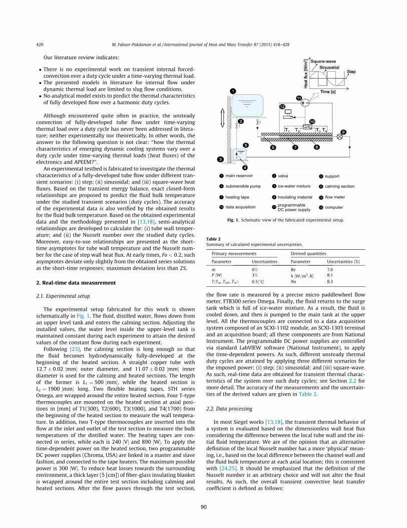
Our literature review indicates:

� There is no experimental work on transient internal forced-convection over a duty cycle under a time-varying thermal load.

� The presented models in literature for internal flow underdynamic thermal load are limited to slug flow conditions.

� No analytical model exists to predict the thermal characteristicsof fully developed flow over a harmonic duty cycles.

Although encountered quite often in practice, the unsteadyconvection of fully-developed tube flow under time-varyingthermal load over a duty cycle has never been addressed in litera-ture; neither experimentally nor theoretically. In other words, theanswer to the following question is not clear: ‘‘how the thermalcharacteristics of emerging dynamic cooling systems vary over aduty cycle under time-varying thermal loads (heat fluxes) of theelectronics and APEEM?’’.

An experimental testbed is fabricated to investigate the thermalcharacteristics of a fully-developed tube flow under different tran-sient scenarios: (i) step; (ii) sinusoidal; and (iii) square-wave heatfluxes. Based on the transient energy balance, exact closed-formrelationships are proposed to predict the fluid bulk temperatureunder the studied transient scenarios (duty cycles). The accuracyof the experimental data is also verified by the obtained resultsfor the fluid bulk temperature. Based on the obtained experimentaldata and the methodology presented in [13,18], semi-analyticalrelationships are developed to calculate the: (i) tube wall temper-ature; and (ii) the Nusselt number over the studied duty cycles.Moreover, easy-to-use relationships are presented as the short-time asymptotes for tube wall temperature and the Nusselt num-ber for the case of step wall heat flux. At early times, Fo < 0:2, suchasymptotes deviate only slightly from the obtained series solutionsas the short-time responses; maximum deviation less than 2%.

2. Real-time data measurement

2.1. Experimental setup

The experimental setup fabricated for this work is shownschematically in Fig. 1. The fluid, distilled water, flows down froman upper level tank and enters the calming section. Adjusting theinstalled valves, the water level inside the upper-level tank ismaintained constant during each experiment to attain the desiredvalues of the constant flow during each experiment.

Following [23], the calming section is long enough so thatthe fluid becomes hydrodynamically fully-developed at thebeginning of the heated section. A straight copper tube with12:7� 0:02 ½mm� outer diameter, and 11:07� 0:02 ½mm� innerdiameter is used for the calming and heated sections. The lengthof the former is L1 ¼ 500 ½mm�, while the heated section isL2 ¼ 1900 ½mm� long. Two flexible heating tapes, STH seriesOmega, are wrapped around the entire heated section. Four T-typethermocouples are mounted on the heated section at axial posi-tions in [mm] of T1(300), T2(600), T3(1000), and T4(1700) fromthe beginning of the heated section to measure the wall tempera-ture. In addition, two T-type thermocouples are inserted into theflow at the inlet and outlet of the test section to measure the bulktemperatures of the distilled water. The heating tapes are con-nected in series, while each is 240 ½V� and 890 ½W�. To apply thetime-dependent power on the heated section, two programmableDC power supplies (Chroma, USA) are linked in a master and slavefashion, and connected to the tape heaters. The maximum possiblepower is 300 ½W�. To reduce heat losses towards the surroundingenvironment, a thick layer (5 [cm]) of fiber-glass insulating blanketis wrapped around the entire test section including calming andheated sections. After the flow passes through the test section,

the flow rate is measured by a precise micro paddlewheel flowmeter, FTB300 series Omega. Finally, the fluid returns to the surgetank which is full of ice-water mixture. As a result, the fluid iscooled down, and then is pumped to the main tank at the upperlevel. All the thermocouples are connected to a data acquisitionsystem composed of an SCXI-1102 module, an SCXI-1303 terminaland an acquisition board; all these components are from NationalInstrument. The programmable DC power supplies are controlledvia standard LabVIEW software (National Instrument), to applythe time-dependent powers. As such, different unsteady thermalduty cycles are attained by applying three different scenarios forthe imposed power: (i) step; (ii) sinusoidal; and (iii) square-wave.As such, real-time data are obtained for transient thermal charac-teristics of the system over such duty cycles; see Section 2.2 formore detail. The accuracy of the measurements and the uncertain-ties of the derived values are given in Table 2.

2.2. Data processing

In most Siegel works [13,18], the transient thermal behavior ofa system is evaluated based on the dimensionless wall heat fluxconsidering the difference between the local tube wall and the ini-tial fluid temperature. We are of the opinion that an alternativedefinition of the local Nusselt number has a more ‘physical’ mean-ing, i.e., based on the local difference between the channel wall andthe fluid bulk temperature at each axial location; this is consistentwith [24,25]. It should be emphasized that the definition of theNusselt number is an arbitrary choice and will not alter the finalresults. As such, the overall transient convective heat transfercoefficient is defined as follows:

Fig. 1. Schematic view of the fabricated experimental setup.

Table 2Summary of calculated experimental uncertainties.

Primary measurements Derived quantities

Parameter Uncertainties Parameter Uncertainties (%)

_m 6% Re 7.6P ½W� 3% h ½W=m2=K� 8.1

TðTin; Tout ; TmÞ 0:5½�C� Nu 8.3


90

hðL2; tÞ ¼ q00ðtÞTwðtÞ � TmðtÞ

ð1Þ

where q00ðtÞ is the applied time-dependent heat flux, TwðtÞ is theaverage tube wall temperature, and TmðtÞ is the arithmetic averageof inlet and outlet fluid bulk temperatures. Therefore, the defini-tions of different parameters in Eq. (1) are given below:

TwðtÞ ¼ 14

X4i¼1

TiðtÞ ð2Þ

TmðtÞ ¼ TinðtÞ þ ToutðtÞ2

ð3Þ

q00ðtÞ ¼ PðtÞpDL2

ð4Þ

where Tin and Tout are the inlet and outlet fluid temperatures,respectively. Moreover, PðtÞ is the applied transient power and L2is the length of the heated section. The overall Nusselt number isalso obtained by the following relationship.

NuDðL2; tÞ ¼ hðL2; tÞ � Dk

ð5Þ

where, D and k are the tube diameter and fluid thermal conductiv-ity, respectively. The thermo-physical properties of the distilledwater used in this study are determined at the arithmetic averagetemperature, TmðtÞ, from [23].

3. Model development

In this section, it is intended to present closed-form solutions forthe thermal characteristics of laminar tube flow under the transientscenarios, i.e., (i) step; (ii) sinusoidal; and (iii) square-wave heatfluxes. Following Siegel [13] and Fakoor-Pakdaman et al. [20,22],closed-form relationships are obtained to calculate: (i) tube walltemperature; (ii) fluid bulk temperature; and (iii) the Nusseltnumber, for the above-mentioned time-dependent heat fluxes.

The methodology presented in [13] proceeds as follows: con-sider a position x in the channel through which the fluid is flowingwith average velocity U. A fluid element starting from the entranceof the channel will require time duration t ¼ x=U to reach the xlocation. In the region where x=U P t, i.e., short-time response,there is no penetration of the fluid which was at the entrance whenthe transient began. Therefore, the short-time response corre-sponds to pure transient heat conduction, and the effect of heatconvection is zero. However, for the region x=U 6 t, the heat trans-fer process occurs via the fluid that entered the channel after thetransient was initiated. This forms the long-time response whichis equal to short time response at the transition time, i.e.,t ¼ x=U. Therefore, the solution composed of two parts that shouldbe considered separately: (i) short-time and (ii) long-timeresponses. More detail regarding the short- and long-timeresponses were presented elsewhere [19–22].

3.1. Step power (heat flux)

For this scenario, the imposed heat flux is considered in thefollowing form:

q00ðtÞ ¼ 0 t < 0q00r ¼ const: t P 0

�ð6Þ

where q00r (offset), is a constant value over the entire heating period.

When a tube flow is suddenly subjected to a step heat flux, theshort-time response for the tube wall temperature is obtained asfollows [12]:

hw ¼ Foþ 18�X1n¼1

e�b2nFo

b2n

ð7Þ

where bn are the positive roots of J1ðbÞ ¼ 0, and J1ðbÞ are the first-order Bessel functions of the first kind, respectively. In addition,hw and Fo are the dimensionless wall temperature and dimension-less time, respectively. Such dimensionless numbers are definedas follows:

hw ¼ Tw � Tin

q00r D=k

; Fo ¼ atR2 ð8Þ

where Tw; Tin; k, and a are tube wall temperature, inlet tempera-ture, fluid thermal conductivity, and diffusivity, respectively. Itshould be noted that when Fo ! 0, Fakoor-Pakdaman andBahrami [26], presented a compact easy-to-use relationship forEq. (7) as the short-time asymptote for the tube wall temperature.For Fo < 0:2, the maximum deviation between the series solution,Eq. (7), and the compact model, Eq. (9), is less than 2%.

hw;Fo!0 ¼ffiffiffiffiffipFo

r� p

4

� �1

ð9Þ

In addition, the long-time asymptote can be obtained by a well-known Graetz solution [25] as given below:

hw ¼ X þ 1148

þ 12

X1n¼1

CnKn exp � k2nX2

!ð10Þ

where X ¼ 4x=DRe�Pr is the dimensionless axial location. Besides, the val-

ues of kn and CnKn are tabulated in [25]. In addition, the fluid bulktemperature can be obtained by performing a heat balance on aninfinitesimal differential control volume of the flow;

_mcpTm þ q00ðpDÞdx� _mcpTm þ _mcp@Tm

@xdx

� ¼ qcp

pD2

4

!@Tm

@tdx

ð11Þ

where _m is the fluid mass flow rate, cp and Tm are specific heat andfluid bulk temperature, respectively. The dimensionless form ofEq. (11) is:

q00ðX; FoÞq00r

¼ @hm@Fo

þ @hm@X

ð12Þ

where q00r is the offset around which the imposed heat flux fluctu-

ates. Eq. (12) is a first-order partial differential equation whichcan be solved by the method of characteristics [27]. The short-and long-time asymptotes for the fluid bulk temperature for thecase of step heat flux are [26];

hm ¼ Fo short� time asymptoteX Long� time asymptote

�ð13Þ

Following Fakoor-Pakdaman and Bahrami [26], the short-timeasymptote for the average Nusselt number under a step heat fluxcan be calculated by a compact relationship, Eq. (14).

NuDðtÞFo!0 ¼ hðtÞ � Dk

¼ffiffiffiffiffipFo

rð14Þ

In addition, the following well-known Shah equation [28] is used asthe long-time asymptote for the average Nusselt number of laminarflow under constant wall heat flux.

Nu0�x;D ¼ 1:953X�1=3 for X 6 0:034:364þ 0:0722

X for X > 0:03

(ð15Þ


91

3.2. Sinusoidal power (heat flux)

For this case, the applied heat flux is considered in the followingform.

q00 ¼ q00r þ a� sin

2pp1

t�

ð16Þ

where, q00r ½W=m2�, a ½W=m2�, and p1 ½s� are the offset, amplitude,

and period of the imposed heat flux. The dimensionless form ofEq. (16) is:

q00

q00r¼ 1þ a

q00r

� � sinðx1FoÞ ð17Þ

where, x1 ¼ 2pR2p1a

is the dimensionless angular frequency of the

imposed heat flux, and R ½m� is the tube radius. SubstitutingEq. (17) into Eq. (12), closed-form relationships are obtained forthe short- and long-time responses for fluid bulk temperature, seeEqs. (18.a) and (18.b). In addition, following the methodology pre-sented in [20], semi-analytical relationships are proposed to predictthe tube wall temperature, Eqs. (19.a) and (19.b). Table 3 presents asummary of the results obtained for short- and long-time responsesof tube wall and fluid bulk temperatures under a sinusoidal heatflux. It should be noted that C1 in Eqs. (19.a) and (19.b), is a coeffi-cient which depends on the velocity profile of the fluid inside thetube. It takes the value of unity for slug flow inside the duct, i.e.,uniform velocity across the tube, see [20]. For a parabolic velocityprofile (poiseuille flow), the value of such coefficient is obtainedin this study empirically, and will be discussed in Section 4, wherethe functions !1;n and !2;n are defined as:

!1;n ¼ e�b2nFo

b2nþx1ða=q00r Þ

x21þb4n

� cosðx1FoÞ� b2nx1

�sinðx1FoÞ�e�b2nFoh i

!2;n ¼ e�b2nX

b2nþx1 ða=q00r Þ

x21þb4n

� cosðx1FoÞ� b2nx1

�sinðx1FoÞþe�b2nX �b2nx1

�sin x1ðFo�XÞ½ ��cos½x1ðFo�XÞ�

( )( )8>>><>>>:

ð18Þ

In addition, the short- and long-time local Nusselt numbers can becalculated by the following relationship:

NuDðx; tÞ ¼ q00D=kTw � Tm

¼ C21þ sinðx1FoÞ

hw � hm

�ð19Þ

Again C2 is a coefficient which takes a value of unity for slug flowinside the duct [20]. The value of such coefficient for a parabolicvelocity in this study is obtained empirically, and discussed inSection 4 of this study. Accordingly, the average Nusselt numberover the entire length of the heated section, L2, is calculated asfollows:

NuDðL2; tÞ ¼ 1L2

Z L2

0NuDdx ð20Þ

3.3. Square-wave power (heat flux)

The Fourier series for a square-wave heat flux with offset q00r ,

amplitude a, and period p2 is, [29]:

q00 ¼ q00r þ a�

X1m¼0;1;2

12mþ 1

sinð2mþ 1Þp

p2t

�ð21Þ

The dimensionless form of Eq. (21) is:

q00

q00r¼ 1þ a

q00r

� �X1

m¼0;1;2

12mþ 1

sinðxmFoÞ ð22Þ

where xm ¼ ð2mþ1ÞpR2p2a

is a dimensionless number which character-

izes the behavior of the square-wave heat flux. SubstitutingEq. (22) into Eq. (12), closed-form relationships are obtained forthe short- and long-time responses for fluid bulk temperature, seeEqs. (25.a) and (25.b). In addition, following the methodologypresented in [20], semi-analytical relationships are proposed topredict the tube wall temperature, Eqs. (26.a) and (26.b). Table 4presents a summary of the results obtained for short- and long-timeresponses of tube wall and fluid bulk temperatures under a square-wave heat flux.

Table 3Tube wall and fluid bulk temperatures for transient scenario II: sinusoidal heat flux, [20].

Short-time response, X 6 Fo Long-time response, X P Fo

Fluid bulk temperature, hm ¼ Tm�Tinq00r D=k

¼ Foþ a=q00rð Þx1

1� cosðx1FoÞ½ � (18.a) ¼ X þ a=q00rð Þx1

cos x1ðFo� XÞ½ � � cosðx1FoÞf g (18.b)

Tube wall temperature, hw ¼ Tw�Tinq00r D=k

¼ C1Foþ a=q00rð Þ

x1� 1� cosðx1FoÞ½ �

þ 18 �

P1n¼1!1;n

( )(19.a) ¼ C1

X þ a=q00rð Þx1

� cos x1ðFo� XÞ½ �� cosðx1FoÞ

� �þ 1

8 �P1

n¼1!2;n

8<:

9=; (19.b)

Table 4Tube wall and fluid bulk temperatures for transient scenario III: square-wave heat flux, Ref. [20].

Short-time response, X 6 Fo Long-time response, X P Fo

Fluid bulk temperature, hm ¼ Tm�Tinq00r D=k

¼ X þ aq00r

� ��P1

m¼0;1;21

xmð2mþ1Þcos xmðFo� XÞ½ �� cosðxmFoÞ

� �(25.a) ¼ X þ a

q00r

� ��P1

m¼0;1;21

xmð2mþ1Þcos xmðFo� XÞ½ �� cosðxmFoÞ

� �(25.b)

Tube wall temperature, hw ¼ Tw�Tinq00r D=k

¼ C2

Foþa=q00r� ��P1

m¼0;1;21

xmð2mþ1Þ �1� cosðxmFoÞ �

þ 18 �

P1n¼1W1;n

8>><>>:

9>>=>>; (26.a) ¼ C2

Xþa=q00rð Þxm

�P1m¼0;1;2

1xmð2mþ1Þ �

cos xmðFo� XÞ½ �� cosðxmFoÞ

� �þ 1

8 �P1

n¼1W2;n

8>><>>:

9>>=>>; (26.b)


92

The functions W1;n and W2;n are defined as:

W1;n ¼ e�b2nFo

b2nþða=q00

r Þ�X1

m¼0;1;2

xm

ð2mþ1Þðx2mþb4n Þ

� cosðxmFoÞ� b2nxm

� sinðxmFoÞ�e�b2nFoh i

W2;n ¼ e�b2nX

b2nþða=q00

r Þ�X1

m¼0;1;2

xm

ð2mþ1Þðx2mþb4n Þ

�cosðxmFoÞ� b2n

xm� sinðxmFoÞþ

e�b2nX �b2nxm

� sin½xmðFo�XÞ��cos½xmðFo�XÞ�

( )8>><>>:

9>>=>>;

8>>>>>>>><>>>>>>>>:

ð23Þ

In addition, the short- and long-time local Nusselt numbers can beobtained by the following relationship:

NuDðx; tÞ ¼ q00D=kTw � Tm

¼ C2

1þ aq00r

� ��P1

m¼0;1;21

2mþ1 sinðxmFoÞhw � hm

24

35 ð24Þ

Similar to Section 3.2, the average Nusselt number over the entirelength of the heated section is:

NuDðL2; tÞ ¼ 1L2

Z L2

0NuDdx ð25Þ

Fig. 2. Short- and long-time asymptotes for outlet fluid bulk-temperature and comparison with experimental data for the step power. ð _m ¼ 3:3� 0:198 ½gr=s�Þ.

Fig. 3. Short- and long-time responses for outlet fluid bulk temperature and comparison with experimental data for the square-wave power. ð _m ¼ 3:6� 0:216 ½gr=s�Þ.


93

4. Results and discussion

4.1. Validation tests/outlet fluid bulk-temperature

Fig. 2 shows the dimensionless short- and long-time asymp-totes, Eq. (13), for the outlet fluid bulk-temperature against thedimensionless time (Fourier number) for a step power. The exactanalytical results are also compared with the obtained experimen-tal data in Fig. 2.

The following highlights the trends in Fig. 2:

� There is an excellent agreement between the exact analyticalsolutions and the obtained experimental data. The maximumrelative difference between the derived asymptotes and theexperimental data is less than 8%.

� The good agreement between the analytical results and theexperimental data verifies the accuracy of the experimentalsetup and the measuring instruments.

� As the heating is applied, the outlet fluid bulk-temperatureincreases to reach the steady-state value at the long-timeasymptote.

� The experimental data show a smooth transition between theshort- and long-time responses.

Fig. 3 depicts the variations of dimensionless outlet fluid bulk-temperature against the Fourier number for a square-wave power.The exact analytical results are also compared with the obtainedexperimental data in Fig. 3. The following conclusions can bedrawn from Fig. 3:

Fig. 4. Short- and long-time responses for outlet temperature and comparison with experimental data for sinusoidal power with different periods: (a) p1 ¼ 400 ½s� and (b)p1 ¼ 50 ½s�. ð _m ¼ 3:6� 0:216 ½gr=s�Þ.


94

� There is a good agreement between the analytical resultsand the obtained experimental data; the maximum relativedifference less than 12%.

� The good agreement between the analytical results and theexperimental data verifies the accuracy of the experimentalsetup and the measuring instruments.

� As the heating is applied, the temperature of the fluid rises toshow steady oscillatory behavior after the transition time,X ¼ Fo. This time is demarcated on Fig. 3 by a vertical dash line.

� There is an initial transient period, which can be considered aspure conduction, i.e., the short-time response for X P Fo.However, as pointed out earlier, each axial position showssteady oscillatory behavior for X < Fo at the long-time response.

� There is a slight discrepancy between the analytical results andexperimental data around the transition time. Referring to[12,20], this happens as a result of the limitations of the math-ematical method ‘‘method of characteristics’’ that is used in [20]to solve the energy equation. Such mathematical method pre-dicts an abrupt transition from short- to long-time responseswhile experimental data show a smooth transition.

� As expected the fluid temperature fluctuates with time in caseof a square-wave heat flux. For a step heat flux, the solutiondoes not fluctuate over time. The temperature fluctuates withthe period of the imposed heat flux.

4.2. Cut-off angular frequency

Fig. 4 shows the dimensionless outlet fluid bulk-temperatureversus the Fourier number under a sinusoidal power. To investi-gate the effects of the angular frequency of the applied heat fluxon the coolant behavior, ‘‘slow’’ and ‘‘fast’’ functions are taken intoaccount for the imposed power. Fig. 4a shows a ‘‘slow’’ transientscenario where the angular frequency of the applied power isp1 ¼ 400 ½s�, while the corresponding value in the ‘‘fast’’ case inFig. 4b is p1 ¼ 50 ½s�. The following highlights the trends in Fig. 4:

� There is a shift between the peaks of the applied power andthe outlet fluid bulk-temperature. This shows a ‘‘thermal lag’’(inertia) of the fluid flow. This thermal lag is attributed to thefluid thermal inertia.

� When a sinusoidal cyclic heat flux with high angular frequencyis imposed on the flow, the fluid does not follow the details ofthe heat flux behavior. Therefore, for very high angular frequen-cies, the fluid flow acts as if the imposed heat flux is constant at‘‘the average value’’ associated with zero frequency for thesinusoidal heat flux.

� For high angular frequencies, i.e., p ! 0orx! 1, the fluidflow response yields that of a step heat flux. This is called the‘‘cut-off’’ pulsation frequency.

� Dimensionless cut-off angular frequency: defined in thisstudy as the angular frequency beyond which the fluidresponse lies within �5% of that of step heat flux. As such,following [22], for a fully developed tube flow subjected to a

sinusoidal wall heat flux, x1 ¼ 2pR2p1a

¼ 15p is the cut-off angular

frequency.� The dimensionless cut-off frequency is a function of heat fluxperiod, p1 ½s�, tube radius, R ½m�, and fluid thermal diffusivity,a ½m2

s �.� Irrespective of Fo number, the amplitude of the dimensionlessfluid bulk-temperature decreases remarkably as the angular fre-quency increases. As mentioned earlier, this happens due to thefact that for high angular frequencies the fluid flow responseapproaches to that of the step heat flux.

4.3. Tube wall temperature

Fig. 5 shows variations of short- and long-time asymptotes fortube wall temperature, Eqs. (7) and (10), against the dimensionlesstime (Fourier number). A comparison is also made in Fig. 6between the presented asymptotes, Eqs. (7) and (10), and theobtained experimental data. Step heat flux, Eq. (6), is imposed onthe tube wall and the experimental data are reported for the ther-mocouples T1 and T4 which are corresponding to axial locationsX ¼ 0:15 and 0:4, respectively. The trends for other axial locationsare similar.


� As heating is applied, the wall temperature rises and then levelsout at a steady state value, i.e., long-time asymptote.

Fig. 5. Short- and long-time asymptotes for tube wall temperature and comparison with experimental data for the step power. ð _m ¼ 3:3� 0:198 ½gr=s�Þ.


95

� There is a good agreement between the experimental data andthe short- and long-time asymptotes, Eqs. (9) and (10); maxi-mum relative difference less than 9.2%.

� The obtained experimental data show a smooth transitionbetween the short- and long-time asymptote.

� Around the transition time, the experimental data branch offfrom the short-time asymptote and plateau out at the long-timeasymptote, Eq. (10).

Fig. 6 depicts the variations of closed-form solutions and exper-imental results for tube wall temperature over the dimensionlesstime (Fourier number) for: (a) sinusoidal power, Eqs. (19.a) and(19.b); and (b) square-wave power, Eq. (26.a) and (26.b). Theexperimental data are reported for the thermocouples T1 and T3

which are corresponding to X ¼ 0:1 and 0:27, respectively. Thetrends for other axial locations are similar. The following highlightsthe trends in Fig. 6:

� There is an initial transient period of pure conduction, i.e.,short-time response, during which all of the curves follow alongthe same line, X P Fo.

� When Fo ¼ X, each curvemoves away from the common line, i. e.,pure conduction responseandadjusts towardsa steadyoscillatorybehavior at long-time response. The transition time for the axiallocations considered in Fig. 6, are indicated by vertical dash lines.

� The wall temperatures become higher for larger X values, asexpected, because of the increase in the fluid bulk temperaturein the axial direction.

� As mentioned before, the value of C1 is unity for slug flow, whileit should be obtained empirically for other velocity profiles.Based on the obtained experimental data, the value of C1 is con-sidered equal to 1.7; in mathematical notation, C1 ¼ 1:7. Assuch, there is an excellent agreement between the closed-formrelationships Eqs. (16) and (22), and the experimental data overthe short-and long-time responses.

Fig. 6. Short- and long-time responses for tube wall temperature and comparison with experimental data for: (a) sinusoidal and (b) square-wave power.ð _m ¼ 3:6� 0:216 ½gr=s�Þ.


96

� There is a small discrepancy between the experimental data andanalytical results around the transition time, X ¼ Fo. Asmentioned before, this is attributed to the limitations of themathematical approach ‘‘method of characteristics’’ that cannotpredict the results around the transition time accurately. Themaximum relative difference between the present analyticalmodel and the experimental data is less than 10.1%.

4.4. Nusselt number

Variations of the average Nusselt number against the Fouriernumber for a step power are depicted in Fig. 7. Short- and long-time responses are shown in Fig. 7, and compared with theobtained experimental data. Moreover, a relationship is proposedas an all-time Nusselt number based on the blending technique[30]. The following can be concluded from Fig. 7:

� There is a good agreement between the short-time asymptote,Eq. (14), and the obtained experimental data at early times,Fo ! 0.

� Around the transition time, the experimental data branch offfrom the short-time asymptote and adjust towards the long-time asymptote.

� Based on the blending technique [31], the following relation-ship is proposed as an all-time model for the average Nusseltnumber under a step heat flux.

NuDðt; xÞ ¼ ½ðNuDðtÞFo!0Þ�3 þ ½Nu0�x;D�3n oð1=3Þ

ð26Þ

where NuDðtÞ and Nu0�x;D are the short- and long-time asymptotes,Eqs. (14) and (15). In addition, NuDðt; xÞ is the all-time modelpresented for the average Nusselt number for a step power.

� The maximum relative difference between the proposedall-time model and the experimental data is less than 7%.

Fig. 8 shows the variations of the average Nusselt numberagainst the Fourier number for the sinusoidal imposed heat flux.Different periods are considered for the imposed power and thesemi-analytical results are compared with obtained experimentaldata. Regarding Fig. 8, the conventional ‘‘quasi-steady’’ model is asimplified model which assumes that the convective heat transfercoefficient is constant, equal to the fully developed condition in thechannel [13]. It should be noted that based on the obtained exper-imental data, the value of the coefficient C2 is considered equal to

0.54. Such value minimizes the difference between the experimen-tal and semi-analytical results; maximum relative difference lessthan 10%. The following highlights the trends in Fig. 8.

� The values of the average Nusselt number vary significantlywith the angular frequency of the imposed heat flux, whilethe conventional models, e.g., quasi-steady model fail to predictsuch variations of the Nusselt number with time.

� The Nusselt number oscillates with the angular frequency of theimposed heat flux.

� Regardless of the angular frequency, at very initial transientperiod, the Nusselt number is much higher than that of thelong-time response.

� The fluctuations of the transient Nusselt number occur some-what around the fully-developed steady-state value.Considering the slug flow inside a circular tube, the value ofthe fully-developed Nusselt number for the steady-state condi-tion is: NuD ¼ 4:36 as predicted by the quasi-steady model [25].

6. Conclusion

An experimental study is carried out to investigate the thermalcharacteristics of a fully-developed tube flow under time-varyingheat fluxes. Three different scenarios are considered for the appliedtime-dependent heat fluxes: (i) step; (ii) sinusoidal; and (iii)square-wave. Exact closed-form relationships are proposed to findthe fluid bulk temperature for the implemented scenarios. As such,the accuracy of the experimental data and the measuring instru-ments are verified. Semi-analytical relationships are proposed topredict; (i) tube wall temperature and (ii) the Nusselt number forall the implemented scenarios. The question ‘‘how the thermalcharacteristics of the dynamic cooling systems vary over a dutycycle’’ is answered here as follows: The imposed heat flux (thermalload) is the dominant parameter that characterizes the thermalbehavior of a cooling system. As such;

� The temperature and the Nusselt number fluctuate with theperiod of the applied thermal load.

� For fast transients, there is a cut-off angular frequency for theimposed heat flux beyond which the fluid does not follow thedetails of the imposed thermal load. The fluid response thenbecomes that of step heat flux.

� The fluid response consists of two main parts: (i) short-timeresponse and (ii) long-time response. The former is correspond-ing to early times during which pure conduction occurs inside

Fig. 7. Short- and long-time responses as well as the proposed all-time model forthe average Nusselt number, and comparison with the obtained experimental datafor the step power. ð _m ¼ 3:3� 0:198 ½gr=s�Þ.

Fig. 8. All-time Nusselt number for sinusoidal transient scenario with differentperiods of p1 ¼ 200 ½s� and p1 ¼ 400 ½s�, and comparison with quasi-steady modeland the obtained experimental data. ð _m ¼ 3:6� 0:216 ½gr=s�Þ.


97

the fluid domain. On the other hand, long-time response refersto a period of time starting after the transition time; the fluidyields steady-oscillatory behavior.

� The conventional steady-state models fail to predict the thermalbehavior of dynamic cooling systems under time-varying ther-mal load.

Conflict of interest

None declared.

Acknowledgments

This work was supported by Automotive Partnership Canada(APC), Grant No. APCPJ 401826-10. The authors would like to thankthe support of the industry partner, Future Vehicle TechnologiesInc. (British Columbia, Canada).

References

[1] M.Marz, A. Schletz, Power electronics system integration for electric and hybridvehicles, in: 6th Int. Conf. Integr. Power Electron. Syst., 2010, pp. Paper 6.1.

[2] K. Chau, C. Chan, C. Liu, Overview of permanent-magnet brushless drives forelectric and hybrid electric vehicles, IEEE Trans. Ind. Electron. 55 (2008) 2246–2257.

[3] J. Garrison, M. Webber, Optimization of an integrated energy storage schemefor a dispatchable wind powered energy system, in: ASME 2012 6th Int. Conf.Energy Sustain. Parts A B San Diego, CA, USA, 2012, pp. 1009–1019.

[4] J. Garrison, M. Webber, An integrated energy storage scheme for a dispatchablesolar and wind powered energy system and analysis of dynamic parameters,Renew. Sustain. Energy 3 (2011) 1–11.

[5] C. Crawford, Balance of power: dynamic thermal management for Internetdata centers, IEEE Internet Comput. 9 (2005) 42–49.

[6] R.R. Schmidt, E.E. Cruz, M. Iyengar, Challenges of data center thermalmanagement, IBM J. Res. Dev. 49 (2005) 709–723.

[7] Y. Joshi, P. Kumar, B. Sammakia, M. Patterson, Energy Efficient ThermalManagement of Data Centers, Springer, US, Boston, MA, 2012.

[8] R. Scott Downing, G. Kojasoy, Single and two-phase pressure dropcharacteristics in miniature helical channels, Exp. Therm. Fluid Sci. 26 (2002)535–546.

[9] S.V. Garimella, L. Yeh, T. Persoons, Thermal Management Challenges inTelecommunication Systems and Data Centers Thermal ManagementChallenges in Telecommunication Systems and Data Centers, CTRC Res. Publ,2012. pp. 1–26.

[10] M. O’Keefe, K. Bennion, A comparison of hybrid electric vehicle powerelectronics cooling options, in: Veh. Power Electron. Cool. Options, 2007,pp. 116–123.

[11] C. Mi, F.Z. Peng, K.J. Kelly, M.O’. Keefe, V. Hassani, Topology, design, analysisand thermal management of power electronics for hybrid electric vehicleapplications, Int. J. Electr. Hybrid Veh. 1 (2008) 276–294.

[12] R. Siegel, Transient heat transfer for laminar slug flow in ducts, Appl. Mech. 81(1959) 140–144.

[13] R. Siegel, M. Perlmutter, Laminar heat transfer in a channel with unsteady flowand wall heating varying with position and time, Trans. ASME 85 (1963)358–365.

[14] R. Siegel, M. Perlmutter, Heat transfer for pulsating laminar duct flow, HeatTransfer 84 (1962) 111–122.

[15] R. Siegel, Heat transfer for laminar flow in ducts with arbitrary time variationsin wall temperature, Trans. ASME 27 (1960) 241–249.

[16] M. Perlmutter, R. Siegel, Two-dimensional unsteady incompressible laminarduct flow with a step change in wall temperature, Trans. ASME 83 (1961)432–440.

[17] M. Perlmutter, R. Siegel, Unsteady laminar flow in a duct with unsteady heataddition, Heat Transfer 83 (1961) 432–439.

[18] R. Siegel, Forced convection in a channel with wall heat capacity and with wallheating variable with axial position and time, Int. J. Heat Mass Transfer 6(1963) 607–620.

[19] M. Fakoor-Pakdaman, M. Andisheh-Tadbir, M. Bahrami, Transient internalforced convection under arbitrary time-dependent heat flux, in: Proc. ASMESummer Heat Transf. Conf., Minneapolis, MN, USA, 2013.

[20] M. Fakoor-Pakdaman, M. Andisheh-Tadbir, M. Bahrami, Unsteady laminarforced-convective tube flow under dynamic time-dependent heat flux, J. HeatTransfer 136 (2014) 041706.

[21] M. Fakoor-Pakdaman, M. Ahmadi, M. Bahrami, Unsteady internal forced-convective flow under dynamic time-dependent boundary temperature,J. Thermophys. Heat Transfer 28 (2014) 463–473.

[22] M. Fakoor-Pakdaman, M. Ahmadi, M. Andisheh-Tadbir, M. Bahrami, Optimalunsteady convection over a duty cycle for arbitrary unsteady flow underdynamic thermal load, Int. J. Heat Mass Transfer 78 (2014) 1187–1198.

[23] F.P. Incropera, D.P. Dewitt, T.L. Bergman, A.S. Lavine, Introduction to HeatTransfer, fifth ed., John Wiley & Sons, USA, 2007.

[24] Z. Guo, H. Sung, Analysis of the Nusselt number in pulsating pipe flow, Int. J.Heat Mass Transfer 40 (1997) 2486–2489.

[25] A. Bejan, Convection Heat Transfer, third ed., USA, 2004.[26] M. Fakoor-Pakdaman, M. Bahrami, Transient internal forced convection under

step wall heat flux, in: Proc. ASME 2013 Summer Heat Transf. Conf. HT2013,2013.

[27] T. Von Karman, M.A. Biot, Mathematical Methods in Engineering, McGraw-Hill,New York, 1940.

[28] R.K. Shah, Thermal entry length solutions for the circular tube and parallelplates, in: Proceeding 3rd Natl. Heat Mass Transf. Conf., Indian Institute ofTechnology, Bombay, 1975, pp. HMT–11–75.

[29] E. Kreyszig, H. Kreyzig, E.J. Norminton, Advanced Engineering Mathematics,10th ed., John Wiley & Sons, n.d.

[30] S.W. Churchill, R. Usagi, A general expression for the correlation of ratesof transfer and other phenomena, Am. Inst. Chem. Eng. 18 (1972) 1121–1128.

[31] R. Siegel, E.M. Sparrow, Transient heat transfer for laminar forced convectionin the thermal entrance region of flat ducts, Heat Transfer 81 (1959) 29–36.


98

mohammad fakoor pakdaman 2015 simon …mbahrami/pdf/theses/thesis m. fakoorpakdaman.pdf ·...

Documents