mol2net 2016, vol. 2, j;

MOL2NET, 2016, Vol. 2, J; http://sciforum.net/conference/MOL2NET-02/SUIWML-01

1

MOL2NET

An Efficient Residual Q-learning Algorithm based on Function Approximation

Hu Wen1,2,3

, Chen Jianping1,2,3

, Fu Qiming1,2,3,4

, Hu Lingyao1,2,3

1) Institute of Electronics and Information Engineering, Suzhou University of Science and Technology, Suzhou，Jiangsu

2) Jiangsu Key Laboratory of Intelligent Building Energy Efficiency, Suzhou University of Science and Technology, Suzhou, Jiangsu

3) Suzhou Key Laboratory of Mobile Networking and Applied Technologies, Suzhou University of Science and Technology, Suzhou, Jiangsu

4) Key Laboratory of Symbolic Computation and Knowledge Engineering of Ministry of Education, Jilin University, Changchun

* Corresponding author email: [email protected]; [email protected]; [email protected]; [email protected]

Abstract: A number of reinforcement learning algorithms have been developed that are guaranteed to converge to the optimal

solution when used with lookup tables. However, these algorithms can easily become unstable when implemented directly

with function approximation. We proposed an efficient Q-learning algorithm based on function approximation (FARQ),

which not only can guarantee the convergence but also has a fast learning rate. The algorithm performs gradient decent on

mean squared Bellman residual and adopts a new rule to update value function parameter vector. In addition, the algorithm

introduces a new factor, named forgotten factor to accelerate the learning rate of the algorithm. Applying the proposed

algorithm, Q-learning, and Actor-Critic algorithm to the traditional Grid World and the pole balancing problems, the

experimental results show that FARQ algorithm has the faster convergence rate and better convergence performance.

Keywords: Reinforcement Learning, Q-learning algorithm, Function Approximation, Gradient Descent, Bellman Residual

1 INTRODUCTION Reinforcement Learning (RL) [1] is considered as a kind of Machine Learning method, which can be applied to handle

problems where the process model is not available in advance. The agent explores an environment and through the use of a

reward signal to maximize the expected cumulative rewards to achieve a certain goal [2]. The traditional RL algorithms

have been guaranteed to converge to the optimal solution, which use the lookup tables to store the value functions for

problems with discrete state and action spaces [3]. The lookup table is generally applied to the problems with small-scale

continuous state space and action spaces, but when dealing with continuous actions, or action space with large discrete sets,

the algorithms will suffer from slow learning rate or even cannot converge. This problem is named the curse of

dimensionality [4], which leads to the increasing computational complexity exponentially with the number of dimensions.

As a result, designing a more efficient algorithm to solve the problem of slow learning rate and unstable converge will be of

great importance in RL.

RL algorithm with function approximation is a new research hotpot in Machine Learning. In the learning process of

algorithms with function approximation, a set of parameters were adopted to describe the state-value function or action-

value function [5-6]. The agent chooses the optimal action according to the approximation, and the learning experiences can

be generalized from the subsets to the whole state space. In the 1990s, Tsitsiklis et al, applied function approximation to RL

algorithms, and the stability and convergence of the algorithms were proved both theoretically and experimentally [6].

SciForum

mailto:[email protected]




2

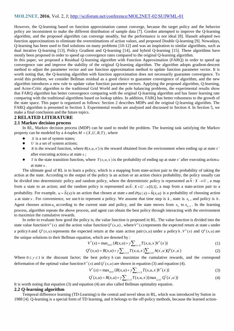
However, the Q-learning based on function approximation cannot converge, because the target policy and the behavior

policy are inconsistent to make the different distribution of sample data [7]. Gordon attempted to improve the Q-learning

algorithm, and the proposed algorithm can converge steadily, but the performance is not ideal [8]. Hasselt adopted two

function approximations to eliminate the overestimations of action values, and proposed Double Q-learning [9]. Nowadays,

Q-learning has been used to find solutions on many problems [10-12] and was an inspiration to similar algorithms, such as

dual iterative Q-learning [13], Policy Gradient and Q-learning [14], and hybrid Q-learning [15]. These algorithms have

mostly been proposed in order to speed up convergence rates compared to the original Q-learning algorithm.

In this paper, we proposed a Residual Q-learning algorithm with Function Approximation (FARQ) in order to speed up

convergence rate and improve the stability of the original Q-learning algorithm. The algorithm adopts gradient-descent

method to adjust the parameter vector and use function approximation method to update function parameter vector. It is

worth noting that, the Q-learning algorithm with function approximation does not necessarily guarantee convergence. To

avoid this problem, we consider Bellman residual as a good choice to guarantee convergence of algorithm, and the new

algorithm introduces a new rule to update value function parameter vectors. Applying the proposed algorithm, Q-learning,

and Actor-Critic algorithm to the traditional Grid World and the pole balancing problems, the experimental results show

that FARQ algorithm has better convergence comparing with the original Q-learning algorithm and has faster learning rate

comparing with the traditional algorithms based on lookup tables. In addition, FARQ has better robustness to the growth of

the state space. This paper is organized as follows: Section 2 describes MDPs and the original Q-learning algorithm. The

FARQ algorithm is presented in Section 3. Experimental results are analyzed and discussed in Section 4. In Section 5, we

make a final conclusion and the future topics.

2 RELATED LITERATURE

2.1 Markov decision process In RL, Markov decision process (MDP) can be used to model the problem. The learning task satisfying the Markov

property can be modeled by a 4-tuples ( , , , )M X U R T , where

X is a set of system states;

U is a set of system actions;

R is the reward function, where ( , , ')R x u x is the reward obtained from the environment when ending up at state 'x

after executing action u at state x ;

T is the state transition function, where '( , , )T x u x is the probability of ending up at state 'x after executing action u

at state x .

The ultimate goal of RL is to learn a policy, which is a mapping from state-action pair to the probability of taking the

action at the state. According to the output of the policy is an action or an action choice probability, the policy usually can

be divided into deterministic policy and random policy, where the deterministic policy is represented as :h X U , a map

from a state to an action; and the random policy is represented as : [0,1]h X U , a map from a state-action pair to a

probability. For example, ( )u h x is an action that chosen at state x and ( | ) ( , )P u x h x u is a probability of choosing action

u at state x . For convenience, we use h to represent a policy. We assume that time step is k , state is kx , and policy is h .

Agent chooses action ku according to the current state and policy, and the state moves from kx to 1kx . In the learning

process, algorithm repeats the above process, and agent can obtain the best policy through interacting with the environment

to maximize the cumulative rewards.

In order to evaluate how good the policy is, the value function is proposed in RL. The value function is divided into the

state value function ( )kV x and the action value function ( , )kQ x u , where ( )kV x represents the expected return at state x under

a policy h and ( , )kQ x u represents the expected return at the state action pair ( , )x u under a policy h . ( )kV x and ( , )kQ x u are

the unique solutions to their Bellman equation, which are denoted by :

'

* ' * '( ) max { ( , ) ( , , ) ( )}u U x XV x R x u T x u x V x

(1)

' '

' ' ' ' '( , ) ( , ) ( , , ) ( , ) ( , )h h

x X u UQ x u R x u T x u x h x u Q x u

(2)

Where 0 1 is the discount factor; the best policy h can maximize the cumulative rewards, and the correspond

deformation of the optimal value function * ( )V x and * ( , )Q x u are shown in equation (3) and equation (4).

'

* ' * '( ) max { ( , ) ( , , ) ( )}u U x XV x R x u T x u x V x

(3)

''

* ' * ' '( , ) ( , ) ( , , ){max ( , )}u Ux X

Q x u R x u T x u x Q x u

(4)

It is worth noting that equation (3) and equation (4) are also called Bellman optimality equation.

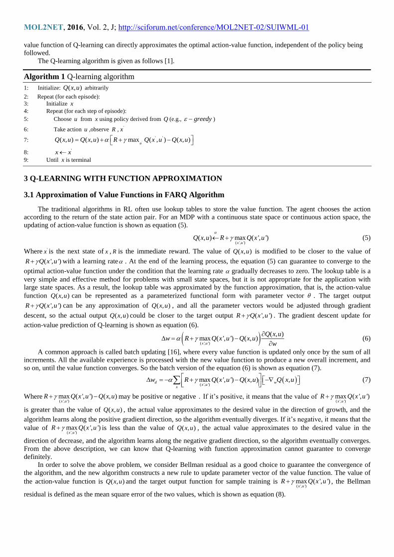
2.2 Q-learning algorithm Temporal difference learning (TD-Learning) is the central and novel ideas in RL, which was introduced by Sutton in

1988 [4]. Q-learning is a special form of TD learning, and it belongs to the off-policy methods, because the learned action-


3

value function of Q-learning can directly approximates the optimal action-value function, independent of the policy being

followed.

The Q-learning algorithm is given as follows [1].

Algorithm 1 Q-learning algorithm

1: Initialize: ( , )Q x u arbitrarily

2: Repeat (for each episode):

3: Initialize x

4: Repeat (for each step of episode):

5: Choose u from x using policy derived from Q (e.g., greedy )

6: Take action u ,observe R ,'x

7: '

' '( , ) ( , ) max ( , ) ( , )u

Q x u Q x u R Q x u Q x u

8: 'x x

9: Until x is terminal

3 Q-LEARNING WITH FUNCTION APPROXIMATION

3.1 Approximation of Value Functions in FARQ Algorithm

The traditional algorithms in RL often use lookup tables to store the value function. The agent chooses the action

according to the return of the state action pair. For an MDP with a continuous state space or continuous action space, the

updating of action-value function is shown as equation (5).

( ', ')

( , ) max ( ', ')x u

Q x u R Q x u

(5)

Where 'x is the next state of x , R is the immediate reward. The value of ( , )Q x u is modified to be closer to the value of

( ', ')R Q x u with a learning rate . At the end of the learning process, the equation (5) can guarantee to converge to the

optimal action-value function under the condition that the learning rate gradually decreases to zero. The lookup table is a

very simple and effective method for problems with small state spaces, but it is not appropriate for the application with

large state spaces. As a result, the lookup table was approximated by the function approximation, that is, the action-value

function ( , )Q x u can be represented as a parameterized functional form with parameter vector . The target output

( ', ')R Q x u can be any approximation of ( , )Q x u , and all the parameter vectors would be adjusted through gradient

descent, so the actual output ( , )Q x u could be closer to the target output ( ', ')R Q x u . The gradient descent update for

action-value prediction of Q-learning is shown as equation (6).

( ', ')

( , )max ( ', ') ( , )

x u

Q x uw R Q x u Q x u

w

(6)

A common approach is called batch updating [16], where every value function is updated only once by the sum of all

increments. All the available experience is processed with the new value function to produce a new overall increment, and

so on, until the value function converges. So the batch version of the equation (6) is shown as equation (7).

( ', ')max ( ', ') ( , ) ,d w

x ux

w R Q x u Q x u Q x u (7)

Where( ', ')max ( ', ') ( , )

x uR Q x u Q x u may be positive or negative．If it’s positive, it means that the value of

( ', ')max ( ', ')

x uR Q x u

is greater than the value of ( , )Q x u , the actual value approximates to the desired value in the direction of growth, and the

algorithm learns along the positive gradient direction, so the algorithm eventually diverges. If it’s negative, it means that the

value of ( ', ')max ( ', ')

x uR Q x u is less than the value of ( , )Q x u , the actual value approximates to the desired value in the

direction of decrease, and the algorithm learns along the negative gradient direction, so the algorithm eventually converges.

From the above description, we can know that Q-learning with function approximation cannot guarantee to converge

definitely.

In order to solve the above problem, we consider Bellman residual as a good choice to guarantee the convergence of

the algorithm, and the new algorithm constructs a new rule to update parameter vector of the value function. The value of

the action-value function is ( , )Q x u and the target output function for sample training is ( ', ')max ( ', ')

x uR Q x u , the Bellman

residual is defined as the mean square error of the two values, which is shown as equation (8).


4

2

( ', ')

1max ( ', ') ( , )

x ux

E R Q x u Q x un

(8)

For the problem with continuous action space, only when the action-value function is optimal, Bellman residual is

zero. By applying the gradient descent method to equation (8) can guarantee E to converge to a local minimum. After the

state x moves to 'x with an immediate reward R , the parameter update vector of Q-learning-Bellman is given by Equation

(9).

( ', ') ( ', ')max ( ', ') , max ( ', ') ,

x u x uw R Q x u Q x u Q x u Q x u

w w

(9)

The difference between Equation (9) and equation (6) is that equation (9) can guarantee the convergence of Bellman

residual, but equation (6) cannot. As a result, applying function approximation to Q-learning algorithm, equation (9) can

guarantee the algorithm to converge to the optimal solution. The batch version of the equation (9) is shown as equation (10).

( ', ') ( ', ')max ( ', ') , max ( ', ') ,rg w w

x u x uw R Q x u Q x u Q x u Q x u

(10)

Where w , rgw , the gradient of ( , )Q x u and ( ', ')Q x u are all vectors. When the step-size parameter satisfies the stochastic

approximation theory [1], rgw can guarantee E to converge to a local minimum. However, comparing with Q-learning

algorithm, Q-learning-Bellman sometimes converges slowly. Take the star problem in Figure 1 as an example. Initialize

5 0w and 4 10w . In the learning process from state 4 to state 5, Q-learning only decreases the value of 4w , but Q-

learning-Bellman increases the value of 5w while decreasing the value of 4w . Therefore, Q-learning-Bellman algorithm will

lead the agent to learning in two directions, and the learning rate will become slower.

Figure 1: The star problem

Q-learning with function approximation has a faster learning rate but cannot guarantee the convergence and Q-learning

with Bellman residual can guarantee the convergence but has a slower learning rate. Considering the two cases, we want to

find an algorithm which not only can guarantee the convergence, but also has a faster learning rate. In figure 3, the dotted

line represents the hyperplane that is perpendicular to the gradient, the above of dotted line represents the negative gradient

direction which causes a decrease in E and the below of dotted line represents the positive gradient direction which causes

an increase in E. The vector rgw is for Q-learning-Bellman, and the vector dw is for Q-learning. The update vector we

need should be as close as possible to dw and still remain to the up of the dotted line, which can guarantee the convergence

Figure 2: Action-value function parameter update vector for FARQ algorithm


5

of the algorithm and make the algorithm learn quickly, such as rw in figure 3. Therefore, the above two value function

parameter vectors are combined with parameter (a constant between 0 and 1), and the new parameter update vector rw

is defined to be:

1r d rgw w w (11)

From the equation (11), we can know that the new vector can ensure the convergence of the algorithm with an appropriate

, because rw causes E to decrease. In addition, the algorithm might have a fast learning rate, because rw lies as close

as possible to dw .

3.2 Selection of in FARQ Algorithm

An important question is how to choose an appropriate in FARQ algorithm. A of 1 is guaranteed to converge,

and a of 0 might be expected to learn quickly. However, both of them are not the best choice, and it requires to analysis

by trial and error.

When the two vectors rw and rgw are orthogonal, then the calculation of would be:

0

((1 ) ) 0

r rg

d rg rg

d rg

d rg rg rg

w w

w w w

w w

w w w w

(12)

If the equation (12) yields a outside of the range 0,1 , then the angel between the vectors rw and rgw is acute. From

figure 3 we can see that the vector rw changes to the above of the hyperplane, which means that the algorithm has

converged, so a of 0 should be used for maximum learning rate in the next learning. When the denominator of is 0,

then the value of is 0, this means that E is at a local minimum, or the vectors rw and rgw point in the same direction.

In either case, the algorithm can guarantee to converge. If the equation (12) yields a between the range 0,1 , then the

value of rgw is 0, which means that E has converged to a local minimum. Theoretically, E will decrease to zero as the

number of iterations increasing, and the algorithm converges eventually. Therefore, any above this value will ensure

convergence. In summary, when satisfies the range[0,1] , the FARS algorithm can guarantee to converge.

In order to make the angle between the two vectors rw and rgw is acute, adding any small, positive constant k to .

Therefore, FARS algorithm should firstly calculate the numerator and the denominator, secondly check whether the

denominator is zero. If the denominator is zero, then is 0. If it is not, the algorithm should evaluate equation (12),

including the addition of a small constant k , then check whether the resulting lies in the range 0,1 . The corresponding

deformation of equation (11) is shown in equation (13).

( ', ')

( ', ') ( ', ')

( ', ') ( ', ')

1

1 max ( ', ') ( , ) ( , )

max ( ', ') ( , ) max ( ', ') ( , )

max ( ', ') ( , ) max ( ',

r d rg

wx u

x

w wx u x u

x

wx u x u

x

w w w

R Q x u Q x u Q x u

R Q x u Q x u Q x u Q x u

R Q x u Q x u Q x

') ( , )wu Q x u

(13)

At the end of an episode, the vectors dw and rgw are updated vectors of the value function parameter in Q-learning and

Q-learning-Bellman respectively. In order to satisfy the requirements of faster convergence, we introduce a new factor (a

small, positive constant) in the updating of dw and rgw , which is named forgotten factor. We use dw and rgw to approximate

dw and rgw , the vectors dw and rgw are updated according to equation (14) and equation (15).

( ', ')

1 max ( ', ') ( , ) ( , )d d wx u

w w R Q x u Q x u Q x u

(14)

( ', ') ( ', ')

1 max ( ', ') ( , ) max ( ', ') ( , )rg rg w wx u x u

w w R Q x u Q x u Q x u Q x u

(15)

In addition, the marginally-stable is calculated by equation (16).


6

+d rg

w

d rg rg

w

w w

w w w

(16)

3.3 FARQ ALGORITHMS

Residual Q-learning Algorithm with function approximation combines the traditional Q-learning algorithm and Q-

learning-Bellman algorithm, which constructs a new method to update parameter vector of action-value function. By

choosing an appropriate and introducing a forgetting factor, the FARS algorithm has better performance and faster

learning rate.

The complete algorithm is given as follows.

Algorithm 2 FARQ algorithm

1: Initialize: 0w ； Xx ；； =0

2: Repeat

3: For each Xx

4: ( , )Q Q x u

5: ( ', ')

( , ) max ( ', ')x u

Q x u R Q x u

6: ( ', ')

1 max ( ', ') ( , ) ( , )d d wx u

w w R Q x u Q x u Q x u

7: ( ', ') ( ', ')

1 max ( ', ') ( , ) max ( ', ') ( , )rg rg w wx u x u

w w R Q x u Q x u Q x u Q x u

8: If 0d rg rg rgw w w w

9: 0

10: Else

11: d rg

w

d rg rg

w

w w

w w w

（）

12: If 1 13: 0

14: Else

15:

16: End If

17: End If

18: ( ', ') ( ', ')max ( ', ') ( , ) max ( ', ') ( , )r r

x u x ux

w w R Q x u Q x u Q x u Q x uw w

19: rw w w

20: 'x x

21: End For

22: Until 0E

4 EXPERIMENTAL RESULTS

In order to verify the effectiveness and performance of the algorithm, the proposed algorithm, Q-learning algorithm, Q-

learning-Bellman algorithm are applied to the classic Windy Grid World and Pole-balancing problems.

4.1 Windy Grid World

We discuss the results of running FARQ, Q-learning, and Q-learning-Bellman algorithms on a 5*6 Windy Grid World

problem, as shown in figure 4. The agent always begins in the square marked ‘S’ and the episode continues until it reaches

the square marked ‘T’. In any state, Agent can choose 4 actions 0 1 2 3, , ,a a a a which represents up, down, left and right as

shown in the direction of the arrow in figure 4. When the column has no wind, the agent chooses an action according to a

state transition, that is, if the agent chooses the right action, the state will move to the right state, and if the agent chooses

the left action, the state will move to the left state. For example, the agent is in the state (3,0) , if the agent chooses the action

to the right, then the state moves to (3,1) . When the column has wind, the resultant next states are shifted upward by the


7

wind. For example, the agent is in state (2,2) , the strength of the wind is 1(The dotted arrow in figure 4 indicates that the

column has wind, and the value above the dotted arrow describes the strength of the wind, such as 0 /1 , which means the

strength may be 0 or 1.), the agent chooses the action to the right, then the state will move to (1,3) . In the process of state

transition, agent can receives a reward of 10 until the goal state is reached, and in other cases, the agent receives a reward of

1. For this experiment, in order to ensure a certain degree of exploration, we adopt greedy method to choose actions. The

maximum number of episodes is set to 250, and the maximum number of time steps of each episode is 2000. The episode

ends means that the agent reaches the goal state or the time step reaches 2000. In addition, we choose regularization

parameter 0.9 , 0.1 , 0.1 and 0.01 .

Figure 3: Windy Grid World problem

Figure 4: Performance analysis for different algorithms on Windy Grid World

Figure 4 shows the performance analysis of Q-learning, FARQ and Q-learning-Bellman algorithms on Windy Grid

World problem. The horizontal axis is the episode, and the vertical axis is the steps for the different algorithms to the goal

state. From figure 4, we can clearly see that the convergence performance of FARQ algorithm is better than the other

algorithms. The three algorithms Q-learning, FARQ and Q-learning-Bellman converge at the 150th, 140

th, and 30

th episodes

respectively. As a result, the FARQ algorithm has the fast convergence rate, possibly due to the introducing of forgotten

factor. In the former episodes, the Q-learning algorithm learns faster than the Q-learning-Bellman algorithm, because the Q-

learning-Bellman algorithm attempts to make each state match both successors and its predecessors, so the learning rate is

slower. In the latter episodes, the Q-learning algorithm fluctuates heavily, and the Q-learning-Bellman algorithm fluctuates

slightly, but the FARQ algorithm does not, that is because the FARQ algorithm combines the traditional Q-learning and

bellman residual method, and introduces a new rule to update the function parameter vector. Evidently, FARQ algorithm

has the best performance.

Figure 5 shows the performance analysis for different of FARQ algorithm on Windy Grid World problem. Figure 6

shows the performance of the latter 100 episodes with different . For each size of training episodes, the date point was

calculated by averaging over 20 times. The horizontal axis is the episode, and the vertical axis is the steps for FARQ

algorithm to reach the goal state. The values of for six lines in figure 6 are 0.001, 0.005, 0.01, 0.05, and 0.2, respectively.

In figure 5, we can clearly see that when 0.001 , 0.005 , 0.01 , 0.05 , and 0.2 the algorithm converges at

about the 125th episode, the 110

th episode, the 90

th episode, the 70

th episode and the 30

th, respectively. As a result, the


8

convergence rate of the algorithm is proportional to the value of . However, when 0.2 , the convergence rate of FARQ

is improved, but the number of the steps to reach the goal state is about 180. Moreover, In figure 6, we can clearly see that

when 0.001 , 0.005 , and 0.05 , the FARQ algorithm fluctuates more heavily than 0.01 . From figure 6, we can

know that when 0.2 , the algorithm converges at a local optimum. Therefore, it is worth noting that the smallest is not

the best . Evidently, an appropriate can make the algorithm have a good robustness and a faster learning rate.

Figure 5: Performance analysis for different of FARQ algorithm on Windy Grid World

Figure 6: Performance analysis for different of FARQ algorithm on Windy Grid World

Figure 7 shows the performance analysis for different of FARQ algorithm on Windy Grid World. For each size of

training episodes, the date point was calculated by averaging over 20 times. Horizontal axis Phi represents the value of ,

and the vertical axis is the steps required for FARQ algorithm to converge. In the simulation result, we can see that when

take different values, the algorithm has different performances. In figure 10, we can know that when 0.2 , the algorithm

has the minimum number step to reach the goal state, and the performance of the algorithm is the best. Moreover, when

0 , the FARQ algorithm and Q-learning algorithm have the same performance, and when 1 , the FARQ algorithm

and the Q-learning-Bellman algorithm also have the same performance. As a result, the Q-learning algorithm and Q-


9

learning-Bellman algorithm are special cases of FARQ algorithm, and the FARQ algorithm can be found that combine the

beneficial properties of both.

Figure7: Performance analysis for different of FARQ algorithm on Windy Grid World

4.2 Pole balancing problem

The pole balancing problem (see Figure 7) requires balancing a pole of unknown length and mass at the upright

position by applying force to the cart it is attached to. At each time step, if the angle m , between the pole and the vertical

line is less than 4 ( 4 ), a reward of 1 will be given; otherwise a reward of -1will be received. The goal is to keep

the pole balance ( 4 ) for a total of 9000 steps during an episode. The maximal episode is 150 and an episode consists

of 9000 time steps. For this experiment, we choose regularization parameter 0.95 , 0.1 , 0.1 and 0.01 . All the

values of the parameters are hand-tuned to obtain the best performance.

Figure 8: The pole balancing problem

The state consists of ( , ) , where 2, 2 is the angel between the pole and the vertical line and 2,2 is

the corresponding angular velocity of the pole. The action u is the force exerting on the cart and its range is

50 ,50u N N . A uniform noise in 10 ,10N N is added to the selected action at each time step. At the start of each

episode, the state of the pole is initialized as (0,0) with a uniform random perturbation. The dynamics of system is shown as

equation (17). 2

2

sinsin cos

4 cos

3

F mlg

m M

ml

m M

(17)


10

Where the gravity constant 29.81g m s , the masses of the pole and the car are 0.1m kg and 1M kg respectively, and the

length of the pole 1l m . Agent exerts the force F to the car, and the time interval is 0.1t , then the state variables are

t and t . The reward function is shown as equation (18).

1 ( , ) 4( , )

1 ( , ) 4

f x ux u

f x u

(18)

We adopt radial basis function (RBF) to extract the features of the states. The center point of the angel and the

angular velocity locate over the grid points -0.75 -0.5 -0.25 0,0.25,0.5,0.75，，， and -2,0,2 , which constitute a total of 21

center points. The variances are 0.2, 2 for and respectively. In pole balancing problem, the performance of the

algorithm is evaluated by the average steps in each episode, and the higher the average steps, the better the algorithm

performance.

Figure 9: Performance analysis for different algorithms on Pole balancing

Figure 9 shows the performance analysis of Q-learning, FARQ and Q-learning-Bellman algorithms on Pole balancing

problem. The horizontal axis is the episode, and the vertical axis is the steps for the different algorithms to the goal state.

The state space is divided into 21 pieces in total, 7 pieces for the angel, and 3pieces for the angular velocity. From figure 9,

Figure10: Performance analysis for different of FARQ algorithm on pole balancing


11

we can note that the performances of the three algorithms differ heavily in all episodes. FARQ tends to converge at the 50th

episode and thereafter it fluctuates slightly. Q-learning and Q-learning-Bellman seem to converge at the 90th and 110

th

episodes, but they fluctuate heavily until the episodes are terminal. Evidently, FARQ algorithm performs best in terms of

convergence rate and stability.

In order to evaluate the effects of for FARQ algorithm on Pole balancing, we choose four different to compare

the performances of FARQ algorithm. the balancing steps are shown in figure 10 respectively. Phi in figure 10 represents

the value of . From four pictures, we can know that when 0.15 , 0.2 , 0.3 , and 0.5 , the FARQ algorithm

converges at the 50th , 50

th ,75

th , and 90

th episodes, respectively. Moreover, when 0.15 , the algorithm fluctuates more

heavily than other three cases after convergence. As a result, when is lager, the convergence rate of FARQ is slower, in

contrast, the convergence rate is improved, but the stability is not the best. Evidently, an appropriate can make the

algorithm have a better performance. Table 1: performance analysis for FARQ algorithm on Pole balancing

0.2 0.3 0.4

0.01 0.1 0.2 0.3 0.01 0.1 0.2 0.3 0.01 0.1 0.2 0.3

MSE 0.28 0.296 0.315 0.342 0.29 0.305 0.323 0.358 0.3 0.318 0.359 0.385

episode 50 45 40 35 75 60 50 40 100 85 80 60

Table 1 is the performance analysis for FARQ algorithm with different and different on Pole balancing problem,

where MSE represents the mean square error of action-value function after convergence of the algorithm, and episode

means the number of episodes when the algorithm converges. From table1, we can clearly see that, when the value of is

constant, as the value of is higher, the convergence rate of the algorithm is faster, but the convergence performance is

worse. When the value of is constant, as the value of is higher, the convergence rate of the algorithm is slower, and

the convergence performance is worse too. Evidently, an appropriate and an appropriate can make the algorithm have

a better performance.

5 CONCLUSIONS This paper proposes an efficient residual Q-learning algorithm based on function approximation, which not only can

guarantee the convergence but also has a fast learning rate. The algorithm combines the traditional Q-learning algorithm and

Bellman residual, and adopts a new rule to update the action-value function parameter vector. Theoretically, the new rule

for updating action-value function parameter vector can guarantee the convergence of the algorithm and solve the unstable

convergence problem of the traditional Q-learning algorithm. To further accelerate the algorithm convergence rate, the

algorithm introduces a new factor, named forgotten factor, which makes the algorithm have a faster learning rate and a good

robustness. We verifies the performance of FARQ on the traditional Windy Grid World and Pole balancing problems,

where we achieve performance exceeding that of both Q-learning and Q-learning-Bellman.

REFERENCES

[1] Sutton R S, Barto A G. Reinforcement Learning: An Introduction. Cambridge: MIT Press, 1998.

[2] Sutton R S. Learning to Predict by the Method of Temporal Differences. Machine Learning, 1988, 3:9-44.

[3] Antos A, Szepesvari C, Mounos R. Learning near-optimal policies with bellman-residual minimization based fitted

policy iteration and a single sample path. Machine Learning, 2008, 71 (1):89-129.

[4] Xiao F, Liu Q, Fu Q M. Gradient descent Sarsa(λ) algorithm based on the adaptive potential function shaping reward

mechanism. Journal of Communications, 2013(1): 77-88.

[5] Sutton R S, McAllester D, Singh S, Mansour Y. Policy gradient methods for reinforcement learning with function

approximation// Proceedings of 16th

Annual Conference on Neural Information Processing Systems. Denver, USA,

2000: 1057-1063.

[6] Tsitsiklis J N, Van Roy B. An analysis of temporal-difference learning with function approximation. IEEE

Transactions on Automatic Control, 1997, 42(5): 674-690.

[7] Baird L C. Residual algorithm: Reinforcement learning with function approximation// Proceeding of 12th International

Conference on Machine Learning. California, USA, 1995: 30-37.

[8] Gordon G J. Stable function approximation in dynamic programming// Proceeding of 12th International Conference on

Machine Learning. California, USA, 1995: 261-268.


12

[9] Hasselt H V. Double Q-learning // Proceeding of the Neural Information Processing Systems. Atlanta: Curran

Associates, 2010: 2613-2621.

[10] Dorigo M, Gambardella L M. Ant-Q: A reinforcement learning approach to the traveling salesman problem [C] In:

Proceedings of ML-95, Twelfth Intern. Conf. on Machine Learning. 2016: 252-260.

[11] Kiumarsi B, Lewis F L, Modares H, et al. Reinforcement Q-learning for optimal tracking control of linear discrete-

time systems with unknown dynamics[J]. Automatica, 2014, 50(4): 1167-1175.

[12] Shamshirband S, Patel A, Anuar N B, et al. Cooperative game theoretic approach using fuzzy Q-learning for detecting

and preventing intrusions in wireless sensor networks[J]. Engineering Applications of Artificial Intelligence, 2014, 32:

228-241.

[13] O'Donoghue B, Munos R, Kavukcuoglu K, et al. PGQ: Combining policy gradient and Q-learning [J]. arXiv preprint

arXiv:1611.01626, 2016.

[14] Wei Q, Liu D, Shi G. A Novel Dual Iterative-Learning Method for Optimal Battery Management in Smart Residential

Environments [J]. IEEE Transactions on Industrial Electronics, 2015, 62(4): 2509-2518.

[15] Narayanan V, Jagannathan S. Distributed adaptive optimal regulation of uncertain large-scale interconnected systems

using hybrid Q-learning approach [J]. IET Control Theory & Applications, 2016.

[16] Barnard, Etienne. Temporal-difference methods and Markov models. IEEE Transactions on Systems, Man, and

Cybernetics 23.2 (1993): 357-365.

[17] Van Hasselt H. Reinforcement learning in continuous state and action spaces [M]. Reinforcement Learning, Springer

Berlin Heidelberg, 2012.

ACKNOWLEDGEMENTS

This paper is supported by National Natural Science Foundation of China (61401297, 61502329, 61602334) and

Natural Science Foundation of Jiangsu (BK20140283).

mol2net 2016, vol. 2, j;

Documents