Molecular Simulation of Chemically

Reacting Flows Inside

Micro/Nano–channels

by

Amir Ahmadzadegan

A thesis

presented to the University of Waterloo

in fulfillment of the

thesis requirement for the degree of

Doctor of Philosophy

in

Mechanical Engineering

Waterloo, Ontario, Canada, 2013

© Amir Ahmadzadegan 2013

I hereby declare that I am the sole author of this thesis. This is a true copy of the thesis,

including any required final revisions, as accepted by my examiners.

I understand that my thesis may be made electronically available to the public.

ii

Abstract

The main objective of this thesis is to study the fundamental behaviour of multi–

component gas mixture flows in micro/nano–channels undergoing catalytic chemical reac-

tions on the walls. This work is primarily focused on nano–scale reacting flows seen in

related applications; especially, miniaturized energy sources such as micro–fuel cells and

batteries. At these geometries, the order of the characteristic length is close to the mean

free path of the flowing gas, making the flow highly rarefied. As a result, non–equilibrium

conditions prevail even the bulk flow and therefore, continuum assumptions are not held

anymore. Hence, discrete methods should be adopted to simulate molecular movements

and interactions described by the Boltzmann equation. The Direct Simulation Monte Carlo

(DSMC) method was employed for the present research due to its natural ability for simu-

lating a broad range of rarefied gas flows, and its flexibility to incorporate surface chemical

reactions.

In the first step, fluid dynamics and the heat transfer of H2/N2 and H2/N2/CO2 gas mix-

ture slip flows in a plain micro–channel are simulated. The obtained results are compared

to the corresponding data achieved from Navier–Stokes equations with slip/jump bound-

ary conditions. Generally, very good agreements are observed between the two methods.

It proves the ability of DSMC in replicating the fluid properties of multi–component gas

mixtures even when high mass discrepancies exist among the species. Based on this com-

parison, the proper parameters are set for the prepared DSMC code, and the appropriate

intermolecular collision model is identified. It is also found that stream variables should be

calculated more accurately at flow boundaries in order to simulate the intense upstream

diffusion emerging at low velocity flows frequently seen in micro/nano–applications. There-

fore, in the second step, a novel pressure boundary condition is introduced for gas mixture

flows by substituting the commonly used Maxwell velocity distribution with the Chapman–

Enskog distribution function. It is shown that this new method yields better results for

lower velocity and higher rarefaction level cases.

In the last step, a new method is proposed for coupling the flow field simulated by

DSMC and surface reactions modelled by the species conservation ODE system derived

from the reaction mechanism. First, a lean H2/air slip flow subjected to oxidation on

iii

platinum coated walls in a flat micro–channel 4µm in height is simulated as a verification

test case. The results obtained are validated against the solutions of the Navier–Stokes

equations with slip/jump boundary conditions and very good conformity is achieved. Next,

several cases undergoing the same reaction with Reynolds numbers ranging from 0.2 to 3.6

and Knudsen numbers ranging from 0.025 to 0.375, are simulated using the verified code

to investigate the effects of the channel height ranging from 0.5µm to 2µm , the inlet mass

flow rate ranging from 5 kg/m2·s to 25 kg/m2·s, the inlet temperature ranging from 300K

to 700K, the wall temperature ranging from 300K to 1000K, and the fuel/air equivalence

ratio ranging from 0.28 to 1.5. Some of the findings are as follows: (1) increasing the surface

temperature from 600K to 1000K and/or the inlet temperature from 300K to 700K results

in negligible enhancement of the conversion rate, (2) the optimum value of the equivalence

ratio is on the fuel lean side (around 0.5), (3) the efficiency of the reactor is higher for

smaller channel heights, and (4) increasing the inlet mass flux elevates the reaction rate

especially for the smaller channels; this effect is not linear and is more magnified for lower

mass fluxes.

iv

Acknowledgements

I am deeply grateful to my supervisors Professor Metin Renksizbulut and Professor

John Wen for their continuous supports and productive instructions during my study.

Their encouraging comments, patience, and sound advices made it possible to overcome

the problems on the way of finishing the present thesis. Metin’s supportive guidances have

always motivated me to continue despite the hardship and move on. I could approach him

without hesitation for help and advice.

I greatly appreciate the efforts of my defence committee members Professors John

Chatzis, Cecile Devaud, and Kyle Daun, who contributed their valuable time to review my

work and helped me fortify the thesis. I am especially thankful to Professor Kyle Daun

for his great help and inspiring comments on my progress in our intermittent meetings

and fruitful time I had as his teaching assistant. I am also sincerely thankful to Professor

Henning Struchtrup for accepting to serve as the external examiner and travelling the long

way from Victoria. I am greatly appreciative of his time and effort dedicated for reviewing

my thesis.

This work was not possible without emotional support of my lovely wife, Saloumeh, who

has filled my life with beauty and happiness since the wonderful moment of meeting her in

the first year of my study. No word can express my gratitude to her patience and kindness

during the last year reviving me with her indulgent smiles through our long–distance

relationship. I am also profoundly indebted to my family for their constant inspiration and

warm supports throughout this long period of time.

I warmly thank all the good friends whose companionship helped me to improve my

personality and caused a delighted time in Waterloo: Amir Haddadzadeh, Madjid Soltani,

Yahya Mahmoodkhani, Mohammad Derakhshani, Keivan Bakhoda, Samad Bazargan, Af-

shin Zamani, and Yasin Hosseinkhani. It was my honour to be the officemate of Azad

Qazi Zade for four years and I really thank him for providing the Navier-Stokes solutions.

I should thank my English tutor and my friend Matthew Zepf for all the productive and

joyful time he devoted voluntarily for our sessions. I am also grateful to Cassie Smith, my

counsellor, for all the invaluable insights I achieved from her constructive advices.

v

Dedication

This is dedicated to my love Saloumeh and my kind family.

vi

Table of Contents

List of Tables x

List of Figures xi

Nomenclature xvi

1 Introduction 1

1.1 Rarefaction . . . . . . . . . . . . . . . . . . . . . . . . . . . . . . . . . . . 2

1.2 Numerical method . . . . . . . . . . . . . . . . . . . . . . . . . . . . . . . 3

1.3 Review of previous studies . . . . . . . . . . . . . . . . . . . . . . . . . . . 6

1.4 Objectives and structure of the thesis . . . . . . . . . . . . . . . . . . . . . 8

2 Direct Simulation Monte Carlo (DSMC) method 10

2.1 Molecular magnitudes . . . . . . . . . . . . . . . . . . . . . . . . . . . . . 11

2.2 DSMC algorithm . . . . . . . . . . . . . . . . . . . . . . . . . . . . . . . . 17

2.2.1 Initialization . . . . . . . . . . . . . . . . . . . . . . . . . . . . . . . 18

2.2.2 Molecular movement . . . . . . . . . . . . . . . . . . . . . . . . . . 21

2.2.3 Intermolecular collisions . . . . . . . . . . . . . . . . . . . . . . . . 21

2.2.4 Sampling and output . . . . . . . . . . . . . . . . . . . . . . . . . . 27

vii

2.3 Boundary conditions . . . . . . . . . . . . . . . . . . . . . . . . . . . . . . 28

2.3.1 Surface interactions . . . . . . . . . . . . . . . . . . . . . . . . . . . 28

2.3.2 Constant surface temperature . . . . . . . . . . . . . . . . . . . . . 28

2.3.3 Inlet and outlet boundary conditions . . . . . . . . . . . . . . . . . 29

3 Non-reacting flows 34

3.1 Number of simulating particles . . . . . . . . . . . . . . . . . . . . . . . . . 35

3.2 Verification against Navier-Stokes . . . . . . . . . . . . . . . . . . . . . . . 35

3.2.1 Problem definition . . . . . . . . . . . . . . . . . . . . . . . . . . . 37

3.2.2 Numerical implementation . . . . . . . . . . . . . . . . . . . . . . . 39

3.2.3 Results and discussion . . . . . . . . . . . . . . . . . . . . . . . . . 41

3.2.4 Summary . . . . . . . . . . . . . . . . . . . . . . . . . . . . . . . . 55

3.3 Effect of higher order pressure boundary conditions . . . . . . . . . . . . . 55

3.3.1 Inlet and outlet boundary conditions . . . . . . . . . . . . . . . . . 58

3.3.2 Numerical verification . . . . . . . . . . . . . . . . . . . . . . . . . 62

3.3.3 Results and discussion . . . . . . . . . . . . . . . . . . . . . . . . . 63

3.3.4 Summary . . . . . . . . . . . . . . . . . . . . . . . . . . . . . . . . 77

4 Heterogeneous catalytic reacting flows in transition regime 78

4.1 Modelling surface catalytic chemical reactions . . . . . . . . . . . . . . . . 78

4.2 Problem definition . . . . . . . . . . . . . . . . . . . . . . . . . . . . . . . 82

4.3 Verifications . . . . . . . . . . . . . . . . . . . . . . . . . . . . . . . . . . . 84

4.4 Results and discussion . . . . . . . . . . . . . . . . . . . . . . . . . . . . . 90

4.4.1 Effect of channel height . . . . . . . . . . . . . . . . . . . . . . . . 94

4.4.2 Effect of equivalence ratio . . . . . . . . . . . . . . . . . . . . . . . 99

viii

4.4.3 Effect of inlet temperature . . . . . . . . . . . . . . . . . . . . . . . 109

4.4.4 Effects of wall temperature . . . . . . . . . . . . . . . . . . . . . . . 114

4.4.5 Effect of mass flux . . . . . . . . . . . . . . . . . . . . . . . . . . . 120

4.5 Summary . . . . . . . . . . . . . . . . . . . . . . . . . . . . . . . . . . . . 132

5 Conclusions and future works 133

Appendices 138

A Evaluation of tensors A, B, and C of the Chapman–Enskog expansion 139

A.1 Evaluation of the tensor B . . . . . . . . . . . . . . . . . . . . . . . . . . . 139

A.2 Evaluation of vectors A and D . . . . . . . . . . . . . . . . . . . . . . . . . 141

A.3 Chapman-Enskog parameters . . . . . . . . . . . . . . . . . . . . . . . . . 143

B Statistical sampling procedure 146

C Navier–Stokes equations with slip–jump boundary conditions 150

C.1 Navier-Stokes equations . . . . . . . . . . . . . . . . . . . . . . . . . . . . 150

References 154

ix

List of Tables

3.1 Properties of single molecules and binary pairs for different species [28]. . . 40

3.2 Geometrical and operational specifications of different cases. . . . . . . . . 43

3.3 Operational parameters of different simulation cases. For all cases, the mix-

ture is 50%-50% by molecular number density, Tw=350K and Tin=300K. . 63

4.1 Surface reaction mechanism for hydrogen oxidation on platinum [58]. Sur-

face species are denoted by a superscript ”*”. . . . . . . . . . . . . . . . . 86

4.2 Surface reaction mechanism for hydrogen oxidation on platinum [58]. Sur-

face species are denoted by a superscript “*”. . . . . . . . . . . . . . . . . 95

A.1 The molecular mass and diameter data used in [49, 50] . . . . . . . . . . . 144

A.2 The comparison of (b−1, b1) calculated from Equation (A.3) with [49] . . . 145

A.3 The comparison of (a−1, a1, d0) calculated from Equation (A.15) and Equa-

tion (A.16) with [50] . . . . . . . . . . . . . . . . . . . . . . . . . . . . . . 145

x

List of Figures

1.1 A conceptual wafer reactor . . . . . . . . . . . . . . . . . . . . . . . . . . . 2

2.1 The flowchart of the DSMC algorithm . . . . . . . . . . . . . . . . . . . . 19

2.2 The solution domain initially divided into cells and sub-cells, and simulating

particles are distributed randomly. . . . . . . . . . . . . . . . . . . . . . . 20

2.3 Demonstration of VHS parameters in molecules A and B collision. . . . . . 23

2.4 A channel connected to an inlet and an outlet reservoirs . . . . . . . . . . 29

2.5 Streamlines for cases (a) P1=1.2bar, and (b) P1=3.0bar . . . . . . . . . . . 30

2.6 Pressure profiles at the inlet of the channel (section 2 of Figure 2.4) and the

pressure value imposed at the inlet of the reservoir (section 1 of the same

figure) for P1=1.2bar and P1=3.0bar . . . . . . . . . . . . . . . . . . . . . 31

3.1 Demonstration of solution independence to number of simulating particles

for sectional distribution of stream velocity at 50% (a) and 75% (b) of the

channel length. The results are shown for the lower half of the channel. . . 36

3.2 The DSMC solution domain which is divided into the microchannel and the

pseudo–reservoir sections of a length r. . . . . . . . . . . . . . . . . . . . . 38

3.3 Velocity slip (a) and wall heat flux (b) compared to the DSMC results of

Liou et al. [13] and Wang et al. [15]. . . . . . . . . . . . . . . . . . . . . . 42

3.4 Slip velocity distribution along the channel obtained from Navier–Stokes

and DSMC methods. ur is the reference velocity (ur = 50m/s). . . . . . . 44

xi

3.5 Normalized slip velocity under different operating conditions specified in

Table 4.2. The reference velocity is ur = 50 m/s. . . . . . . . . . . . . . . . 45

3.6 Distributions of x–component (a) and y–component (b) of the stream veloc-

ity across the channel at three locations along the channel for case 1. . . . 47

3.7 Normalized slip velocity and the wall Knudsen number in a H = 4µm channel. 48

3.8 Hydrogen and nitrogen mass fractions across the channel at x/H = 0.259

for case 1. . . . . . . . . . . . . . . . . . . . . . . . . . . . . . . . . . . . . 49

3.9 Velocity slip (a) and temperature jump (b) predictions for case 1 with dif-

ferent pseudo–reservoir lengths. ur=50m/s . . . . . . . . . . . . . . . . . . 50

3.10 Velocity slip (a) and mass fractions of H2/N2/CO2 at x/H = 0.157 (b) for

the gas mixture of Case 6 . . . . . . . . . . . . . . . . . . . . . . . . . . . 52

3.11 Temperature discontinuity at the edge of the Knudsen layer under different

operating conditions. . . . . . . . . . . . . . . . . . . . . . . . . . . . . . . 53

3.12 Wall heat flux along the channel under different operating conditions; The

results of Case 1 are multiplied by 0.5 to avoid cluttering. . . . . . . . . . . 54

3.13 The schematic of the channel under study . . . . . . . . . . . . . . . . . . 59

3.14 Verification of velocity and temperature cross-sectional profiles for Case 1

against Wang et al. [15] reported at x/Lc = 0.1 (”” from Maxwell, ”∗”from Chapman-Enskog and continuous line [15]) and x/Lc = 0.7 (”M” from

Maxwell, ”×” from Chapman-Enskog and dash line [15]). . . . . . . . . . . 64

3.15 Comparison of (a) wall heat flux and (b) pressure distribution obtained from

DSMC/M and DSMC/CE for Case 1 with Wang et al. [15] (negative heat

flux represents heat being extracted from the wall). . . . . . . . . . . . . . 65

3.16 Variations of ∆N = N−DSMC − N (0)− relative to N (0)− along the channel for

Case 2; N−DSMC is the number flux calculated by DSMC and N (0) the one

calculated from DSMC/M crossing the vertical face of the cells adjacent to

the walls. . . . . . . . . . . . . . . . . . . . . . . . . . . . . . . . . . . . . 67

xii

3.17 Pressure and Kn distributions for higher speed cases, i.e. Case 1 and Case

2; (M) and (C) represent the results of DSMC/M and DSMC/CE respectively. 68

3.18 The contour plot of the number density of He in gas mixture flow of He-N2

for Case 2; thicker line: DSMC/M and thinner line: DSMC/CE . . . . . . 69

3.19 Contour plots of the He concentration for two extended channels with dif-

ferent Lext of (a) 5.0µm and (b) 6.0µm and properties of Case 2. . . . . . . 70

3.20 Contour plots of the He concentration calculated from DSMC/M (thinner

lines, lower half), DSMC/CE (thicker lines, lower half), and the reference

data (upper half) for (a) Case 3 and (b) Case 4. . . . . . . . . . . . . . . . 71

3.21 Variations of pressure and Kn along the mid-plane of the channel for lower

speed cases, i.e. (a) Case 3 and (b) Case 4. . . . . . . . . . . . . . . . . . . 72

3.22 Velocity slip (a) and pressure variations (b) along the channel wall for Case

2 based on the Maxwell distribution (DSMC/M), the Chapman-Enskog dis-

tribution(DSMC/CE), and the reference data (DSMC/R). . . . . . . . . . 74

3.23 The variation of ∆N = N− − N (0)− relative to N (0)− along the channel for

(a) Case 2 and (b) Case 4; N (0)− is the number flux calculated from the

Maxwell (DSMC/M) distribution. . . . . . . . . . . . . . . . . . . . . . . . 76

4.1 Different states of molecular collisions with the wall. This figure shows four

particles initially located in two boundary cells and hitting a surrounding

wall. If the collision is sampled based on initial position, particles 1 and 2

are considered to hit the wall inside cell ”a” and as well particles 3 and 4

for will be considered for cell ”b”. However, if the collision is sampled based

on the collision spot on the surface, particles 1 and 3 will be sampled for

cell ”a” and particles 2 and 4 are sampled for cell ”b”. Obviously the latter

method should be used to evaluate MCR correctly. . . . . . . . . . . . . . 80

4.2 Variations of surface coverage of surface species; (a) Oxygen ”O” and plat-

inum ”Pt”, (b) Hydrogen ”H”, Hydroxyl ”OH”, and Water ”H2O” . . . . . 87

4.3 Consumption/Production rate of gas species on the catalytic surface. Posi-

tive and negative values denote consumption and production respectively. . 88

xiii

4.4 Variations of the slip velocity, gas temperature next to the wall and pressure

at midplane of the channel. . . . . . . . . . . . . . . . . . . . . . . . . . . 89

4.5 Variations of molar concentration of gas species; (a) N2, (b) H2, O2, and H2O 91

4.6 Sectional verification of gas species mole fractions . . . . . . . . . . . . . . 92

4.5 Sectional verification of gas species mole fractions (continued) . . . . . . . 93

4.6 (a) Mass flux of fuel/air and water at the inlet of the channel. (b) Mass

concentration of fuel/air species at the inlet of the channel. Solid lines

represent mass concentrations calculated from the specified equivalence ratio 96

4.7 Effects of geometry on flow properties; Cases 5-7 . . . . . . . . . . . . . . . 97

4.8 Effects of geometry on θH∗ and XH2 ; Cases 1-4 . . . . . . . . . . . . . . . . 100

4.9 Effects of geometry on θO∗ and XO2 ; Cases 1-4 . . . . . . . . . . . . . . . . 101

4.10 Effects of geometry on θH2O∗ and XH2O; Cases 1-4 . . . . . . . . . . . . . . 102

4.11 Effect of geometry on conversion rate of H2; Cases 1-4 . . . . . . . . . . . . 103

4.12 Effect of geometry on molar flow rate of H2 through the channel; Cases 1-4 103

4.13 Effects of geometry on θOH∗ ; Cases 1-4 . . . . . . . . . . . . . . . . . . . . 104

4.14 Effects of equivalence ratio on θH∗ and XH2 ; Cases 4–8 . . . . . . . . . . . 106

4.15 Effects of equivalence ratio on θO∗ and XO2 ; Cases 4–8 . . . . . . . . . . . 107

4.16 Effects of equivalence ratio on θH2O∗ and XH2O; Cases 4–8 . . . . . . . . . 108

4.17 Effects of equivalence ratio on θOH∗ ; Cases 4–8 . . . . . . . . . . . . . . . . 109

4.18 Effects of geometry on θH∗ at stoichiometric and fuel rich conditions . . . . 110

4.19 Effects of geometry on θO∗ at stoichiometric and fuel rich conditions . . . . 111

4.20 Effects of geometry on θH2O∗ at stoichiometric and fuel rich conditions . . . 112

4.21 Effects of inlet temperature on surface coverages; Cases 4, 9, and 10 . . . . 113

4.22 Effects of wall temperature on θH∗ and XH2 . . . . . . . . . . . . . . . . . 116

4.23 Effects of wall temperature on θO∗ and XO2 . . . . . . . . . . . . . . . . . 117

xiv

4.24 Effects of wall temperature on θH2O∗ and XH2O . . . . . . . . . . . . . . . . 118

4.25 Effects of wall temperature on θOH∗ . . . . . . . . . . . . . . . . . . . . . . 119

4.26 Effects of wall temperature on the conversion rate of H2 . . . . . . . . . . 119

4.27 Effects of the wall temperature on θH∗ at stoichiometric conditions. . . . . 121

4.28 Effects of the wall temperature on θO∗ at stoichiometric conditions. . . . . 122

4.29 Effects of the wall temperature on θH2O∗ at stoichiometric conditions. . . . 123

4.30 Effects of the wall temperature on θH∗ at fuel rich conditions. . . . . . . . 124

4.31 Effects of the wall temperature on θO∗ at fuel rich conditions. . . . . . . . . 125

4.32 Effects of the wall temperature on θH2O∗ at fuel rich conditions. . . . . . . 126

4.33 Molar flow of H2O at different Tw under stoichiometric and fuel rich conditions.127

4.34 Effects of mass flux on θH∗ and XH2 . . . . . . . . . . . . . . . . . . . . . . 128

4.35 Effects of mass flux on θO∗ and XO2 . . . . . . . . . . . . . . . . . . . . . . 129

4.36 Effects of mass flux on θH2O∗ and XH2O. . . . . . . . . . . . . . . . . . . . 130

4.37 Effects of mass flux on molar flow of H2 . . . . . . . . . . . . . . . . . . . 131

xv

Nomenclature

General Symbols

Av Avogadro’s number

~Fb Body force vector

f Velocity distribution function

k The Boltzmann constant (m2 · kg · s−2 ·K−1)

Kn Knudsen number

m′′i Mass flux of the species i (kg ·m−2 · s−1)

m Molecular mass (kg)

mr Reduced mass

Ma Mach number

Ni Molecular number flux of the species i (m−2 · s−1)

n Number density (m−3)

P Pressure tensor

p Pressure (Pa, bar=105Pa)

xvi

pr Pressure ratio

~q Heat transfer vector (W )

R Specific gas constant (J · kg−1 ·K−1)

Rf Random number

Re Reynolds number

Sn Number of real molecules represented by each particle

T Temperature (K)

Ts Gas temperature next to the wall (K)

Tw Wall temperature (K)

u,v,w Components of the velocity vector v (m/s)

v Velocity (m/s)

v′ Molecular thermal velocity (m/s)

v0 Mean stream velocity (m/s)

Vmp Most probable thermal velocity (m/s)

Xi Molar fraction of species i

Yi Mass fraction of species i

Greek Symbols

β Reciprocal of the most probable velocity

Γ Density of catalytic free sites (m−2)

γi Sticking factor of the species i

xvii

δ Mean molecular spacing

δ Unity tensor

ζ Internal degrees of freedom

θi Surface coverage of the species i

λ Mean free path (m)

νf Mean collision frequency (s−1)

ρ Density (kg ·m−3)

σ Molecular diameter (m)

σT Collision cross section

φ Air/fuel equivalence ratio

ω Temperature exponent in the viscosity expression (viscosity index)

Subscripts

0 Mean stream values

in Inlet

int Internal

n Normal component

out Outlet

ref Reference value

tr Translational

x, y Cartesian directions

xviii

Acronyms

DSMC Direct Simulation Monte Carlo

DSMC/CE DSMC results with pressure boundary condition derived from Chapman–

Enskog velocity distribution

DSMC/M DSMC results with pressure boundary condition derived from Maxwell ve-

locity distribution

HS Hard Sphere collision model

MCR Mean Collision Rate

NS Navier–Stokes solution

NSWS/J Navier–Stokes solution with slip/jump boundary conditions

VHS Variable Hard Sphere collision model

VSS Variable Soft Sphere collision model

xix

Chapter 1

Introduction

This thesis is dedicated to a fundamental study of gas mixture flows through flat micro/nano–

channels undergoing chemical reactions on catalytic walls. The method introduced in this

research can be used in developing future continuous flow micro/nano–reactors as a part

of many progressing technologies in which catalytic walls are involved. Of the various ap-

plications, miniaturized sources of energy is mainly targeted in this thesis and is the base

for choosing chemical reactions and gas species utilized in the problems studied. These

energy sources are especially beneficial for next generations of electronic devices and micro

electro–mechanical systems (MEMS) not only because of their very small sizes, but also

for their durability. Developing such technologies would able their users, for example to

have their cell phones on for days with just a drop of a fuel.

Another direction of the research followed in this thesis is focusing mostly on nano–

scale reactors. A conceptual reactor can be assumed as a wafer type reactor consisting

of several micro–reactor layers with similar arrangements as shown in Figure 1.1. As

seen, a perforated plate is sandwiched between two plenums; one reserved for the inlet

and the other for the outlet. The height of these plenums is considered well below the

quenching distance in order to prevent any combustion outside the catalytic channels in the

perforated plate. The inlet plenum provides a fuel/air mass flow, min, with an equivalence

ratio, φ. The homogenized fuel/air mixture enters the inlet plenum and eventually flows

through the perforations in the plate. As shown in Figure 1.1 each perforation makes a

1

Figure 1.1: A conceptual wafer reactor

channel with a low height–to–width aspect ratio and with platinum coating on its walls.

Therefore, the flow through the plate can be simulated as flow through a bundle of parallel

channels and flow through each of these channels can be simulated as flow between parallel

walls. Analyzing these reactors can also help to have better understanding the behavior of

catalytical–chemical reactions in nano–porous media used in fuel cells and nano–channel

reactors if the proper reaction mechanism is implemented. In order to attain this goal,

it is necessary to understand all physical phenomena associated with micro/nano–scale

reactors. A detailed experimental analysis which can capture variations in flow and surface

properties along a micro/nano–reactor seems extremely difficult for the time being, based

on current measurement technologies. Therefore, reliable numerical analysis is the only

method that can be used for this purpose and is undertaken in the present work.

1.1 Rarefaction

Generally, the miniaturization of flow geometries intensifies non-equilibrium effects close

to the walls and even in the bulk flow. This happens due to the fact that as the size of flow

passages approach the mean molecular spacing, the number of molecules in the confined

space decreases, assuming a constant pressure. As a result, the ratio of the mean collision

rate of the molecules with the surrounding walls and the intermolecular collision rates de-

part from their equilibrium values. This hinders the information transfer between surfaces

2

and the flowing gas leading to some specific behaviours such as velocity slip, temperature

jump, and concentration jump. These non-equilibrium phenomena are similar to that seen

in low density conditions associated with low pressure environments and therefore, called

rarefaction. The level of rarefaction depends on the characteristic size of the channel (h)

and the mean free path of the flowing gas (λ). Thus, it is typically described by the ratio

λ/h known as the Knudsen number Kn, based on which, micro-gas flows fall into four

categories: continuum flow (Kn < 0.0051), slip flow (0.005 < Kn < 0.1), transition flow

(0.1 < Kn < 10), and free molecular flow (Kn > 10). Conventional partial differential

models like Navier-Stokes equations are only valid for the continuum flow regime. In the

slip flow regime, bulk motion is still in equilibrium; however, non–equilibrium conditions

arise between the wall surface and the adjacent gas flow. Therefore, Navier-Stokes equa-

tions can still be used for simulating the bulk motion (outside of the Knudsen layer) in

the slip flow regime, and the discontinuity at the gas–wall interface is modelled by taking

advantage of slip/jump boundary conditions. For the rest of the Kn range, however, the

flow is fully rarefied and discrete molecular methods should be employed. In modelling

free molecular flows (Kn > 10), it is assumed that the intermolecular collisions are so rare

that they can be completely neglected. This simplifies the simulation to just modelling

molecular advection and hence, many related problems can be solved analytically. In the

case of the transition flow regime (0.1 < Kn < 10) however, intermolecular collisions are

important and as well, continuum methods are inapplicable. The Kn range associated with

gas nano–flows, which are of interest in this thesis, mostly fall in this regime. In order to

solve transition flow problems, atomistic modelling techniques known as direct simulation

methods must be employed.

1.2 Numerical method

At the molecular scale there is an uncertainty associated with every measured quantity.

This issue has been established by Heisenberg based on the fact that the probability of a

definite value for a molecular quantity at those scales is zero; therefore, for every quantity,

1Different criteria can be found in the literature for continuum flow from 0.001 [1] to 0.01 [2]

3

there must be a differential range in which a certain value would be possible. Accordingly,

in discrete methods, kinetics of the probability density function f(~r,~v, t) of the molecules

located at ~r with a velocity of ~v are analysed. The Boltzmann equation introduced by

Ludwig Eduard Boltzmann (1844 – 1906) is the cornerstone of the kinetic theory of gases

and describes the general distribution of f(~r,~v, t) (the definition of f is given in (2.5)) for

dilute gases: [1]

δ

δt(nf) + ~v · δ

δ~r(nf) + ~Fb ·

δ

δ~v(nf) =

∞∫−∞

4π∫0

n2(f ∗f ∗1 − ff1)vrσ(vr,Ω)dΩd~v1 (1.1)

where, σ is the collision cross–section and ~Fb represents external body forces. The left

hand side of the Boltzmann equation describes effects of the molecular convection, while

its right hand side describes effects of intermolecular collisions.

A direct solution for the Boltzmann equation is too costly and time consuming, espe-

cially when complicated phenomena like chemical reactions are involved. Therefore, differ-

ent methods have been developed to reduce the required computational effort. Theoretical

solutions are also very restricted to some simple cases, mostly for the free molecular regime.

Generally, they simplify the Boltzmann equation either by linearization and simplification

of the collision integral [3, 4], or by using distribution functions and Chapmann-Enskog

expansion [5, 6]. Although these solutions are analytical, due to errors associated with

linearizations and simplifications, they are not of adequate accuracy. In addition, final

partial differential equations obtained from such methods still require numerical solution.

Full numerical solutions, on the other hand, can handle majority of problems with

reasonable accuracy. A group of such numerical methods solve the Boltzmann equation

directly by linearizing and discritizing it over a generated mesh distributed over the entire

solution domain. Some of these methods split the Boltzmann equation into two parts:

transport terms and collision terms. They treat the former just the same as the finite dif-

ference method and handle the latter using the Monte Carlo algorithm. Another old but

efficient numerical scheme is the discrete ordinate method; in which, the molecular velocity

is restricted to predefined values and directions [7, 8]. The most successful method of this

group is the Lattice–Boltzmann method (LBM), which presents a different approach for

4

modelling both continuum and discrete fluid flows. However, due to the complicated per-

turbed derivation of the LBM, simulation of complex phenomena such as thermal radiation

or chemical reaction becomes prohibitively difficult; especially, where steep gradients are

present [9, 1].

The remaining type of numerical methods to solve the Boltzmann equation are catego-

rized as direct simulations, which model molecular translations and collisions stochastically.

Molecular Dynamics (MD) method and Direct Simulation Monte Carlo (DSMC) are the

two commonly used direct simulation methods. In the MD method molecules occupy space

and intermolecular forces are considered in detail. Using the resultant force exerted on each

molecule, molecular translations are traced according to Newtons second law, and dynamic

and kinematic relations. As can be inferred from the nature of the MD procedure, the in-

tention is to mimic the actual molecular physics and geometry. Therefore, the number of

simulating molecules for achieving reasonable accuracy and meaningful averages is high

and not arbitrary. In fact, this number should be identical to those inside a cube with

dimensions equal to one mean free path λ. Hence, this number is obtained from:

NMD = nλ3 (1.2)

In standard conditions, this number is nearly 108 for a cubic domain with 30λ. The point

is that the mean free path is proportional to ρ−1 and consequently λ ∝ n−1, and thus,

NMD ∝ n−2 and it can be seen that if the pressure is raised to 100 times its standard

magnitude, the required number of molecules in the specified cube reduces to 104. The

MD method, therefore, is suitable for higher pressures since the computation load is lower

at those conditions. In the rarefied gas flow, however, working pressure is typically low

and/or λ is comparable to the characteristic length of the domain; these conditions are not

necessarily in favour of the MD method.

The DSMC method, on the other hand, is specially developed to stochastically model

rarefied gas flows, where fundamental assumptions are based on low density gases and ideal

gas relations. Molecules are modelled by so–called simulating particles (so–called particles

throughout this thesis), which are assumed unaware of each other, unless there is a collision.

The DSMC was introduced by G.A. Bird in 1963 and is known to be a remarkably successful

tool in modelling complicated physical phenomena in rarefied gas flows. It is, in fact, the

5

only numerical method currently available to deal with high Kn rarefied gas flows [2]. The

specifications and capabilities of the DSMC method get along well with the requirements

of the current study and therefore, it is employed as the numerical method. Like all other

numerical models, there are some drawbacks associated with DSMC : DSMC is generally

considered a demanding numerical method and its computational time is much longer than

conventional CFD methods even for a simple geometry flow. Due to the stochastic nature

of the DSMC method, the results contain some statistical scatter. This reduces the quality

of the results especially in low velocity flows where the order of the statistical scatter of a

variable is close to its actual value. In such a case, the number of iterations required to

decrease the statistical scatter to a reasonable level can be so high that DSMC method

becomes inefficient. Moreover, as it will be shown in this work, an appropriate treatment

of open boundary conditions has not been well defined yet, especially for gas mixtures,

and using extended domains are still necessary to minimize the imperfections at the flow

inlet/outlet boundaries.

1.3 Review of previous studies

The DSMC method is naturally able to deliver physical phenomena such as pressure and

thermal diffusion which are difficult to capture by continuum transport models [10]. There-

fore, DSMC has been undertaken by researchers for simulating gas flows in micro/nano–

channels. Most of the studies, however, has been devoted to single component gas flows.

One of the very first attempts is an inlet/outlet pressure boundary condition introduced by

Ikegawa and Kobayashi [11]. They simulated a Poiseuille flow in the transition regime with

a Kn range between 0.13 to 5 and verified mass flux results at different Knudsen numbers

against experimental data. Their method of controlling pressure, however, uses flow infor-

mation collected from the last time step which increases the instability and amplifies the

statistical scatter. Piekos and Breuer [12] introduced a modified pressure boundary con-

dition using the characteristic line method and substituting for the unknown variables at

flow boundaries the corresponding weighted average values of the last several time–steps.

They simulated gas flows in a parallel micro–channel in the slip and transition regimes and

their findings demonstrate the intrinsic ability of DSMC to capture the non–equilibrium

6

phenomena at moderate to high Knudsen numbers. In the verification of their results

with analytical data, small errors together with high fluctuations are observed. Liou et

al. [13] and Wang et al. [14] improved the pressure boundary condition using gas dynam-

ics relations and obtained accurate results with reasonably less statistical scatter even in

the velocity field. They compared velocity slip from DSMC simulations with theoretical

results for a range of Knudsen numbers 0.05 < Kn < 1. In their work, the temperature

distribution and the effect of Knudsen number on the heat transfer characteristics of such

flows are also investigated. Wang et al. [15] introduced a constant heat flux boundary

treatment scheme for DSMC modelling of micro–channel flows. Based on this method, the

wall surface temperature is evaluated at each time step using the specified heat flux and

the total energy (translational and internal) of the incident molecules.

Less focus has been devoted to multi–component gaseous flows in micro–channels al-

though majority of applications are of this type. A proper implementation of the pressure

boundary condition is especially a challenge at the flow boundaries. A simple workaround

is leaving the boundary untreated. This reproduces the vacuum environment at the bound-

ary causing considerable pressure drop and large stream velocities close to the boundary.

Le and Hassan [16] applied this method at the outlet boundary in their study of the mixing

process of CO and N2 in a T-shaped micro–mixer. Wang and Li [14] studied the parallel

mixing process of the same species in a planar channel. They imposed constant pressure

at the outlet boundary, however, CO/N2 species have almost the same molecular mass and

diameter and therefore, the procedure used for single component flows can still be applied.

Yan and Farouk [17] studied the flow of binary mixtures of He/Xe, He/Kr and He/Ar.

They utilized the method originated by Piekos and Breuer [12].

Wang et al. [15] used mixtures of various species in their attempt to propose a constant

heat flux boundary treatment. However, the inlet/outlet pressure ratio they applied was

so high that the outlet velocity passes sonic threshold and hence, no molecule enters at the

boundary; this way, no special treatment is required for the outlet boundary.

Working with individual molecules makes DSMC an efficient and flexible method for

simulating gas mixtures flows exposed to chemical reactions. Bird [18] introduced a model

based on the reactive cross section for simulating binary reactions. In that model, exper-

imental kinetics in the form of the Arrhenius equation were translated into a probability,

7

by which some intermolecular collisions result in chemical reactions. Later on, Bird intro-

duced an alternative model based on the collision energy and the vibrational energy levels

of the reactant molecules participating in the collision [18]. The latter eliminates the de-

pendency on experimental kinetics. Another method is called the Macroscopic Chemistry

Method (MCM) introduced by Lilley and Macrossan [19]. In this method, instead of using

the reactive cross section, mean values of species concentrations are directly substituted

into the Arrhenius equation associated with each sub-reaction, and thus, chemical kinet-

ics with a large number of sub-reactions and species can be modelled easier. However,

as part of their procedure, it is required to artificially compensate the chemical potential

of the reactants, by adding it in the form of internal or translation energy to the prod-

uct molecules. This leads to irregular molecular velocities and results in instabilities for

micro/nano–applications which have mostly low temperatures. All of the above mentioned

methods, however, have been introduced for homogeneous gas reactions. Heterogeneous

chemical reactions are seldom investigated by DSMC. Few reported studies, like Cercignani

et al. [20], deal with simple dissociation reactions without catalytic effects.

1.4 Objectives and structure of the thesis

The main objective of this thesis is to develop a comprehensive DSMC code to simulate

chemically reacting gaseous flows inside micro/nano–planar channels with greater focus on

nano–scales using the least simplifying assumptions. The DSMC method and its algorithm

is briefly described in Chapter 2. In addition, many parameters from gas dynamics and

statistical mechanics required in understanding DSMC routines are explained in Section 2.1

in the same chapter. General forms of thermal and fluid dynamics boundary conditions

used in DSMC are discussed in this chapter. The method introduced in this thesis for

coupling heterogeneous reactions on the catalytic walls and the flow is also included.

The first step prior to modeling chemical reacting flows is to develop a code for sim-

ulating non–reacting multi–component micro/nano–flows and to verify the results in de-

tail. In Section 3.2 of Chapter 3 the fluid dynamics and thermal results obtained from

the DSMC code are verified against the solutions of the Navier-Stokes equations with

8

slip/jump boundary conditions for gaseous micro–flows in the slip flow regime. The re-

sults of this study have been published in the International Journal of Heat and Mass

Transfer [21]. As stated before, proper implementation of flow boundary conditions, espe-

cially the pressure boundary condition is a challenge for modeling gas mixture flows using

DSMC. Moreover, stream velocities are generally low in micro/nano–channel applications

and therefore, upstream diffusion is important. This can carry the inaccuracies, produced

by an inefficient outlet pressure boundary condition, upstream into the channel and affect

the flow properties. Therefore, in Section 3.3 of Chapter 3 a through review of available

pressure boundary conditions is presented and then an improved pressure boundary con-

dition using the Chapman–Enskog distribution is introduced. It is shown that this new

pressure boundary treatment can improve the accuracy of the results for high Kn and

low inlet/outlet pressure ratio cases. The results of this section have been published in

International Journal of Modern Physics C [22].

In Chapter 4, the procedure of modeling heterogeneous chemical reactions by DSMC

is implemented and the achieved results are verified against Navier-Stokes equations with

slip/jump boundary treatment. The chosen problem is the H2/air gas mixture flow with

a specified equivalence ratio in a planar micro–channel undergoing catalytic oxidation on

platinum coated walls. It should be noted that the oxidation of H2 undertaken in this

study is an example and the general method of Chapter 4 is capable of modeling other

surface reactions as long as their mechanism is known. The validated code is then used

to study the same reacting flow under different geometrical and fluid dynamics conditions.

This way, effects of the channel height, inlet mass flow rate, inlet and wall temperatures,

and the equivalence ratio are investigated.

Finally in Chapter 5 conclusions are discussed and the possibilities for future works are

suggested.

9

Chapter 2

Direct Simulation Monte Carlo

(DSMC) method

As mentioned, conventional Navier-Stokes equations are only valid for continuum flows.

They can also be used for simulating the bulk motion (outside the Knudsen layer) in the

slip flow regime, taking advantage of slip/jump conditions to model the rarefaction effects

which appear on the walls. For the rest of the Kn range, however, the flow is fully rarefied

and atomistic modelling techniques must be employed.

The Direct Simulation Monte Carlo method satisfies the Boltzmann equation [23] us-

ing a stochastic approach and is applicable for a broad range of Kn from slip flow to

free molecular flow. Although DSMC is computationally demanding, particularly in low

velocity and low Kn flows, alternative methods [24] (e.g., Grad’s 13-moment, linearised

Boltzmann, extended lattice Boltzmann) have limitations on the Kn range and are not all

flexible enough to include complex phenomena such as chemical reactions. Theoretically,

there is no limitation on Kn for DSMC and this especially makes DSMC a proper method

for modelling nano-scale flows. In addition, high Kn conditions are favourable for the

DSMC algorithm and improves its efficiency at nano-geometries.

The DSMC algorithm is based on the collision theory in which, molecular movements

and intermolecular collisions are the only calculations made for modelling a gas flow. The

collision models have been under improvement since first versions of DSMC were published.

10

The simplest model is the Hard Sphere (HS) model in which post–collision velocities of a

colliding pair of molecules have the same distribution as of two hard spheres with the same

geometries and pre–collision specifications. This model has been improved to include the

effects of short range forces and anisotropic scattering as seen in reality using a phenomeno-

logical approach. As a result some more realistic models have been introduced; Variable

Hard Sphere (VHS) model by Bird [1], Variable Soft Sphere (VSS) model by Koura and

Matsumoto [25, 26], and Generalised Hard Sphere (GHS) model by Hassan and Hash [27].

In case of an intermolecular collision, the internal energy is also exchanged as well as the

translational energy. When introduced, the DSMC method was based on the Chapman-

Cowling [28] gas kinetic theory. The strength point of Chapman-Cowlings theory in con-

trast to others, was taking the benefit of Larson-Borgnakke [29] procedure of intermolecular

energy exchange during inelastic collisions. In addition, unlike other methods that devote

their focus on modelling the collisions all theoretically in detail, Larson-Borgnakke model

presented a phenomenological approach. This avoids most of the difficulties associated with

storing data associated with the molecular orientation and rotational speed, and eliminates

the need for complicated computations.

Many parameters are involved in the DSMC procedure, both from statistical mechan-

ics and gas dynamics. A selected number of these parameters which are important in

understanding the DSMC procedure are briefly explained in the next section.

2.1 Molecular magnitudes

Generally, any vector or scalar quantity which is a function of molecular speed ~v are

considered as molecular properties [28]. These properties can be functions of time or

position as well. As expected, molecular properties have erratic changes both in time

and in space, which is due to the variations of the number of the molecules inside the

considered volume during the time. Consequently, time average (average of a quantity

over a relatively long period of time) and ensemble average (average over an indefinite

number of calculation repetitions) are used to demonstrate a mean value. The average

values or symbols presented in this thesis are ensemble averages unless otherwise stated.

11

An ensemble average value is generally defined as follows:

Q = ΣQ/∆N (2.1)

In which, ΣQ is the summation of any molecular quantity Q for a finite number of molecules

∆N which is calculated by n∆V for a finite volume ∆V , and Q is the corresponding mean

value. The integral form of ensemble averaging is:

Q =1

N

∫QdN (2.2)

The common classical model that generally expresses molecular interactions is the inverse

power law model which describes the long range force between two molecules:

F = κ/rn (2.3)

in which, r is the distance between the center of the molecule.

There are two main assumptions that are essential for DSMC simulation of molecular

collisions; first, the flowing gas is dilute i.e., the distance between two molecules is much

greater than the molecules diameter, d. Second, the period of time for each collision can

be neglected. The average volume occupied by a single molecule in a gas with a number

density of n is:

δ3 = n−1 (2.4)

Based on this definition, dilute gases can be recognized by the criterion of δ >> d (con-

versely δ/d >7 [30]).

According to uncertainties at molecular scales, each molecule is in a position between

~r and ~r + ~dr with a velocity of ~v + ~dv. Hence, a probability distribution function can be

defined for the number of molecules with a specific location and velocity as follows [1]:

dN = nf(~v, ~r, t).dv.dr (2.5)

in which dN is the number of molecules located between ~r and ~r+ ~dr and having a velocity

between ~v and ~v + ~dv. The relative velocity of two molecules with velocities ~v1 and ~v2 is:

~vr = ~v1 − ~v2 (2.6)

12

Another important definition is for the thermal velocity given by:

~v′ = ~v − ~v0 (2.7)

where, ~v0 represents the stream velocity vector. Nearly all intensive macroscopic quantities

such as temperature, are directly related to the thermal velocity.

As stated previously, the simplest intermolecular collision model is HS in which, each

molecule is assumed as a solid sphere with a diameter of d. Now, one can consider an

imaginary circle around a molecule of radius d. A collision happens whenever the trajectory

of another molecule crosses this circle. Such a circle is called total collision cross section

σT which is equal to πd2/4 for the HS model but in reality, σT depends on vr as well.

σT is an important quantity in the simulation of macroscopic properties of the flowing

gas such as viscosity and diffusion coefficients. In the HS model, trajectories of deflected

molecules come from a fixed center of scattering which makes all deflection angles equally

likely. More realistic models are described in Section 2.2.3. Assuming HS for collisions of

the molecules with uniform diameter, the average number of intermolecular collisions seen

by each molecule in a time interval ∆t is [1]:

νf = nσTvr (2.8)

Using the result of Equation (2.8), a simple relation can be derived for the mean free path

λ as follows:

λ =v′

νf=

1

n (σTvr/v′)(2.9)

In addition, the average period of time between two successive intermolecular collisions of

one molecule known as mean collision time (∆tc) is obtained from:

∆tc = 1/νf (2.10)

Using the quantities defined so far, it is possible to evaluate the number of intermolecular

collisions in a unit of volume during a unit of time as:

Nc =1

2nνf =

1

2n2σTvr (2.11)

13

This relation is the base of the No Time Counter (NTC) DSMC method which will be

explained later.

In the rest of this section, some expressions used in the final sampling step are presented.

The pressure tensor P (the negative of the conventional stress tensor introduced in fluid

mechanics) is defined as [1]:

P = ρ~v′~v′ (2.12)

Scalar pressure used in the transport equations is then defined as:

p =1

3ρ~v′

2(2.13)

Since heat transfer and chemical reactions are part of the current study, the quantities

required for non–isothermal analysis are presented here. The kinetic energy of a molecule

due to its translational motion with its thermal velocity is:

Etr =1

2mv′2 (2.14)

The distribution of the molecular energy based on the Larsen–Borgenakke theory is as

follows [1]:

fEtr ∝ Etr3/2−ω exp−Etr/(kT ) (2.15)

It is common to denote the quantity Etr/m by etr called specific translational energy.

Combining equations Equations 2.13 and 2.14 results in:

p =2

3ρetr (2.16)

Comparing the result with the ideal gas relation p = ρRT which is applicable for equilib-

rium conditions, it is possible to define a translational kinetic temperature Ttr as:

etr =3

2RTtr (2.17)

Internal energy temperature is defined in the same way for diatomic and poly-atomic

molecules. Different modes of internal energy like rotational and vibrational energies are

possible for a molecule according to its structure and number of atoms. The distribution

of Eint is written as [1]:

fEint∝ Eint

ζ/2−1 exp−Eint/(kT ) (2.18)

14

Similar to the expression of translational energy (Equation 2.17) an internal energy tem-

perature Tint can be defined in such a way that:

eint =1

2ζRTint (2.19)

where eint = Eint/m. In equilibrium conditions; all internal and translational temperatures

are equal for the molecules located in a dV . For gases in non-equilibrium conditions the

measurable temperature at a point is defined as [1]:

T = (3Ttr + ζTint)/(3 + ζ) (2.20)

In molecular approach, heat flux is the summation of translational energy (12ρv′2~v′), and

internal energy (ρeint~v′) of the molecules passing a unit area of a surface; therefore:

~q =1

2ρv′2~v′ + ρeint

~v′ (2.21)

It is worth to note that 3p = ρv′2 from Equation 2.13, so that the first term in the above

equation is related to the pressure work on moving molecules.

All quantities defined above are for single–component gases. the equivalence of some of

these quantities are presented for multi–component gas mixtures, due to their importance

in this study. Total amount of a gas mixture molecules located in a unit of volume is:

n =s∑i=1

ni (2.22)

where, s is the total number of species. As such, the density of a gas mixture is evaluated

from:

ρ =s∑i=1

nimi = nm (2.23)

If species 1 and 2 are selected, then the effective molecular diameter is considered as:

d12 = (d1 + d2)/2 (2.24)

The corresponding collision cross section is:

σT 12 = πd212 (2.25)

15

If it is considered that molecules of species 1 are colliding with those of species 2, the mean

collision rate of the selected pair of species can be obtained from:

νf 12 = n1σT 12vr12 (2.26)

where, σT 12 = πd212 and in the HS model, d12 = (d1 + d2)/2. The collision rate for each

species can be determined by summation of Equation (2.26) over all species:

νf i =s∑j=1

(njσT ijvrij

)(2.27)

The same as single gas, the mean free path is calculated from Equation 2.9 by substituting

mean collision rate from equation Equation 2.27:

λi =

(s∑j=1

(niσT ijvrij/v′i

))−1

(2.28)

The total number of collisions per unit time and per unit volume can then be obtained

from:

Nc =1

2nνf =

1

2

s∑i=1

(niνf i

)(2.29)

The mean values of some flow variables used in sampling routines are presented here.

The stream velocity is obtained from [31]:

~v0 =1

ρ

s∑i=1

(mini~vi

)(2.30)

In which, ~vi is the average of molecular velocities for the species i. The pressure tensor

and scalar pressure are:

Pxy =s∑i=1

(ρiv′xiv′yi

)(2.31)

p = −1

3

s∑i=1

(ρiv′

2i

)(2.32)

16

where, x and y are components of the vector ~v′i and xy indicates the components of the

stress tensor σ. The mean translational temperature for the mixture is:

3

2kTtr =

1

2

s∑i=1

(ni/n)miv′

2i

(2.33)

For diatomic and polyatomic gases, a definition similar to Equation 2.19 is applicable for

each species. For the gas mixture, mean internal degrees of freedom is defined, so that the

definition of the internal energy temperature is:

1

2ζRTint =

s∑i=1

nineinti (2.34)

Similarly, a component of the heat flux is expressed as:

qx =∑[

1

2ρiv′

2i v′xi + ρieintiv

′xi

](2.35)

2.2 DSMC algorithm

DSMC decouples the Boltzmann equation (Equation (1.1)) into two parts: molecular move-

ment and intermolecular collisions. These parts are respectively applied to simulating par-

ticles each representing a specified number, Sn, of real molecules. In the DSMC method,

the domain is first partitioned into some virtual cells which are used to trace the movement

of simulating particles. The simulating particles are initially spread over the cells and their

initial velocities are assigned from the equilibrium distribution. New particles enter at the

inlet and outlet boundaries and the simulating particles move according to their existing

velocities during the time step ∆t. The time step must be chosen in such a way that a

molecule with the maximum molecular speed cannot traverse a cell face at once. The max-

imum molecular speed is considered as three times the most probable molecular thermal

speed Vmp of the species involved [1]. The expression of Vmp is as follows:

Vmp =

(2kT

m

)−1/2

(2.36)

17

where, k is the Boltzmann constant and m denotes the molecular mass. Those molecules

which collide with the walls are reflected according to the condition considered for the

walls. After finishing the movements, a specific number of pairs from the molecules in each

cell are then randomly selected for binary collisions. Following Bird’s NTC methodology

[1], intermolecular collisions take place between some of the pairs according to a specified

probability. The post-collision particle velocities and translational directions are then

calculated and saved.

After a specific number of movement and collision loops, velocity, translational energy,

and internal energy of the simulating particles inside each cell are sampled and thus, one

iteration is completed. This iteration is repeated for a specific number, and then the values

of number density, pressure, mass averaged stream velocity and temperature for each cell

are calculated as final outputs using the information sampled during the solution and the

equations provided in Section 2.1. These quantities are also calculated for implementation

of the inlet and outlet boundary conditions as required, similar to the DSMC-IP procedure

[32]. The cell-based data preservation is known as an efficient way to reduce statistical

scatter [32]. As outlined above, DSMC algorithm consists of four steps (see Figure 2.1):

1. Initialization

2. Molecular movement

3. Intermolecular collision

4. Sampling and output

2.2.1 Initialization

Initially, the domain is partitioned into virtual cells which are demonstrated in Figure 2.2.

The cell based scheme is an efficient method of tracing incremental movement of large

number of particles which is used in the DSMC. The cell side length, ∆x, must be a

fraction of the mean free path. As it was noted by Bird [1], ∆x should be less than λ/3.

18

Figure 2.1: The flowchart of the DSMC algorithm

19

Figure 2.2: The solution domain initially divided into cells and sub-cells, and simulating

particles are distributed randomly.

The maximum limit of ∆t is calculated based on ∆x as follows:

∆t < C∆x/Vmp (2.37)

The value of C is normally taken equal to 0.1 [33]. In the modified version of the DSMC

(1994 & 2007), each cell is also divided into uniform sub-cells (see Figure 2.2). This way,

binary collision partners are chosen from the molecules inside each sub–cell and therefore,

they are closer to each other and more likely to collide. Furthermore, sub-cells are not

considered in sampling steps for the sake of saving computation time and memory and

hence, this approach is superior to using finer cells [34]. At the beginning, simulating

molecules are randomly spread out among the cells, with an equilibrium velocity distribu-

tion (Maxwellian velocity distribution) as follows:

f (0) = V −3mp π

−3/2 exp(−v′2/V 2

mp

)(2.38)

All of them are numbered and their positions are traced by the corresponding sub-cell and

the cell numbers they are in. Sampling a random value from a distribution is the basis

for the Monte Carlo methods which is demonstrated in Appendix B. Using this sampling

20

procedure, values of velocity components for 2D problems are initialized as:

A =√−ln(Rf1)

θ = 2πRf2

vx = A cos(θ)

vy = A sin(θ)

(2.39)

where Rf1 and Rf2 are two randomly generated numbers between 0 and 1. In this step

initial values of species mole fractions are also set to the specified values at the inlet of the

channel.

2.2.2 Molecular movement

The simulating particles are moved with regard to their existing velocities during the

time interval ∆t. Interactions with the walls are performed in this step as well which is

described in Section 2.3. In the cell based scheme, following the moving procedure, there

is an indexing routine which sorts the molecule numbers in cells and sub-cells. Algorithm

of such a procedure is simple in the case of a single gas flow; however, for gas mixtures,

numbering logic must support binary collisions of both similar and different species.

2.2.3 Intermolecular collisions

In this step, first, pairs of molecules are selected randomly within sub–cells. The total

number of collisions in a cell during ∆t simply equals to Nc∆t; where, Nc is obtained from

Equation 2.11. The number of selected pairs, however, should be higher since not all of the

selected pairs collide with each other. Therefore, in the No Time Counter method (NTC)

proposed by Bird [1], this number is calculated according to the collision probability Pc.

Pc is based on the product of relative velocity and collision cross section which implies a

cylinder with the cross section σT swept by a molecule towards another, so that the length

of the cylinder will be vr · ∆t. The collision happens whenever a molecule exists in the

swept volume, σTvr ·∆t. Therefore, the collision probability Pc is obtained from [1]:

Pc = vrσT/(vrσT )max (2.40)

21

The initial value of (vrσT )max is set to a suitably large magnitude and is updated during

the solution. The total number of collision during one ∆t , therefore, is calculated from

Equation (2.29). In the NTC method, this value is divided by the collision probability,

Equation 2.40, to obtain the total number of binary pairs which should be considered to

account for the actual number of binary collisions. The result is:

Nsel =1

2NcellN cellSn(vrσT )max∆t/Vcell (2.41)

in which, Sn is the number of real molecules represented by a simulating particle, Ncell

is the average number of simulating particles in a cell and N cell is the time average of

the Ncell. Equation 2.41 reveals that Nsel varies linearly with Ncell, using the relation

N2cell = NcellN cell. This is one of the main advantages of Bird’s NTC method. The

collision probability Pc is then checked for each selected pair and the collision happens if

a random number Rf is larger than Pc. Values of post-collision translational and internal

energies are then required to be evaluated for successful collision pairs. This is done through

the collision model employed in the simulation.

Elastic binary collisions

A binary collision is elastic if only translational energy is exchanged during the collision. In

this case, to obtain post–collision velocities, momentum and energy conservation equations

are to be solved; however, two extra equations are required to calculate all velocity compo-

nents. Hence, the azimuth angle, ε (see Figure 2.3), and the center distance, b, are usually

prescribed by a collision model. As it was mentioned in Section 2.1, the HS model cannot

express the physics of the collision completely and therefore, VHS (Variable Hard Sphere)

and VSS (Variable Soft Sphere) models have been introduced. VHS is a generalized form

of the HS model with the same fixed center of scattering but variable diameter d. In the

VHS model, d is not constant but a function of the vr. Such a relation is of this form [31]:

σT/σT,ref = (d/dref )2 = (vr/vref )−2ζ (2.42)

The reference values of dref and σt,ref are specified at a reference relative velocity, vref . In

this model b is related to the deflection angle χ as:

b = d · cos(χ/2) (2.43)

22

Figure 2.3: Demonstration of VHS parameters in molecules A and B collision.

The deflection angle is then calculated from cos(χ) = 2(b/d)2/α − 1. In the above relation

d is the effective diameter and thus, a collision takes place if the fraction b/d falls within 0

and 1. Theoretically, any choice in the range of 0 to 1 is probable for the quantity b/d, as

a result, in the Monte-Carlo methodology a random number will be chosen in this range

and accordingly, the angle of deflection is calculated from:

cos(χ) = 2(Rf )2 − 1 (2.44)

where Rf is a random number in the range 0 to 1. In addition the angle between the

collision plane and the reference plane, ε, can vary between 0 and 2π; therefore, ε/2π falls

within 0 and 1 and is treated similar to b/d as:

ε = 2πRf (2.45)

The collision cross section of VHS model is independent of deflection angle χ. There-

fore, all reflection angles are of the same probability (fixed center of scatter) so that the

orientation of the reference plane is not important. In such a condition, it is preferred to

consider the x axes parallel to the direction of −→vr and one of the other axes is placed in

23

the collision plane. According to Figure 2.3 and using momentum and energy balances of

the colliding molecules, the magnitudes of the post–collision velocities for the VHS model

are obtained as [31, 1]:

v∗rx = vr cosχ

v∗ry = vr cos ε · sinχv∗rz = vr sin ε · sinχ

(2.46)

Here, vr represents the pre-collision and v∗r represents the post–collision relative velocities.

The VHS model does not follow the inverse power law for modelling short range forces

due to its fixed scattering center. Therefore, Koura and Matsumoto [25] made the following

modification (the VSS model):

b = d · cosα(χ/2) (2.47)

In the VSS model both the diameter d and the exponent α are obtained from the inverse

power law model. This way, a phenomenological method is presented for obtaining phys-

ical scattering deflection angles. Magnitudes of α depend on temperature and molecular

properties of the collision partners. In the VSS model, a reference plane is fixed in an

arbitrary position for all collision calculations. This plane is usually chosen normal to one

of the global axes. Consequently, the deflection angle is sampled from:

cos(χ) = 2(Rf )2/α − 1 (2.48)

and the velocities components are given by:

A = cosχ

B = sinχ

C = cos ε

D = sin ε

E =√v2ry + v2

rz

v∗rx = Avrx + E ·B ·Dv∗ry = Avry + (C · |vr|vrz −D · vrxvry)B/Ev∗rz = Avrz − (C · |vr|vry +D · vrxvrz)B/E

(2.49)

Due to computational demand of VSS model, it is used only if α − 1 > 10−3; otherwise,

VHS model is preferred. Elastic collisions are limited mostly to single atomic molecules

24

which have just one internal degree of freedom, ζ = 1. Nevertheless, diatomic and poly-

atomic molecules are always involved in chemically reacting flows. During collisions of such

molecules internal energy is exchanged as well as translational energy.

Inelastic binary collisions

During inelastic collisions, there is an exchange of energy between both translational and

internal modes. In order to maintain equilibrium conditions, energy must be distributed

appropriately among these modes. The Larson–Borgnakke redistribution model is an ef-

fective method for this purpose and is undertaken in DSMC. Translational and internal

energy distribution functions are presented in Equations 2.15 and 2.18 respectively. The

total collision energy is the sum of translational and internal energies of both molecules.

It can be shown that the probability ratio of a certain amount of translational energy [1]

is:P

Pmax=

ζ + 1/2− ω

3/2− ω

(EtrEc

)3/2−ω ζ + 1/2− ω

ζ − 1

(1− Etr

Ec

)ζ−1

(2.50)

With regard to the form of the above relation, Bird introduced a phenomenological form

of Larson–Borgnakke model, applicable for general poly-atomic energy interchange, based

on Pullins theory [35]. Generally, total number of internal degrees of freedom for both

collision partners is:

Σζ = (5/2− ω12) + ζrot,1/2 + ζrot,2/2 + Σζv,1/2 + Σζv,2/2 (2.51)

It was stated in Section 2.1 that in the inverse power law model, viscosity varies with

temperature as:

µ ∝ T ω12 (2.52)

where ω12 = 12(η + 3)/(η − 1) and η is the exponent of Equation 2.3. If Σζ is divided

into two parts, Σζa and Σζb, the distribution of energy between them according to Larsen–

Borgnakke methodology is:

f

(Ea

Ea + Eb

)= f

(Eb

Ea + Eb

)=

Γ(Σζa + Σζb)

Γ(Σζa)Γ(Σζb)

(Ea

Ea + Eb

)Σζa−1(Eb

Ea + Eb

)Σζb−1

(2.53)

25

By integrating the last equation from zero to one with respect to the variable Ea/(Ea + Eb),

the following result is obtained for the mean value of Ea which is distributed equally

between its all degrees of freedom:

Ea =Σζa

Σζa + Σζb(Ea + Eb) (2.54)

The Larsen–Borgnakke method allows redistribution to be brought about in successive

steps. Consequently, the rotational energy redistribution can be analysed independently.

To redistribute rotational energy, Σζb is set to the total translational degrees of freedom:

Σζb = 5/2− ω12 (2.55)

Unlike the original Larsen–Borgnakke method, a fraction of collisions, Ω, is assumed to be

completely inelastic. The fraction Ω is also called collision number which is a second order

function of macroscopic temperature in real gases. A random number, Rf , is generated

and if 1/Ω > Rf , the rotational energy is to be redistributed. Such a criterion must be

checked for both colliding molecules separately, since it is possible that rotational energy

redistribution takes place only in one of the partners. In this condition, the chosen molecule

rotational degrees of freedom is added to Σζa; so that, all degrees of freedom from which

energy of collision is to be redistributed to Σζa, are stored in Σζb. Moreover, the energy

of collision is translational energy plus total rotational energy of one or both interacting

molecules (depending on the redistribution condition). Now, it is required to calculate the

ratio Ea/(Ea + Eb). Following the Monte-Carlo procedure, the probability of an amount of

energy equal to Ea is associated with Σζa. This quantity is obtained from Equation (2.57)

as:

P

Pmax=

(Σζa + Σζb − 2

Σζa − 1

(Ea

Ea + Eb

))Σζa−1(Σζa + Σζb − 2

Σζa − 1

(1− Ea

Ea + Eb

))Σζb−1

(2.56)

As it is not possible to get inverse from the last equation (in order to have a straight forward

relation for the Ea/(Ea + Eb) ratio), an acceptance-rejection procedure is applied which

is explained in Appendix B. In such a procedure, a random number Rf1 is generated and

P/Pmax is calculated by substituting Rf1 in place of the ratio Ea/(Ea + Eb) in equation

Equation (2.56). Then Rf1 is accepted if P/Pmax > Rf2; in which, Rf2 is a second random

number between zero and one.

26

In the special case of just two internal degrees of freedom for rotational energy, the

ratio Ea/(Ea + Eb) is obtained easier from the following relation:

EaEa + Eb

= 1−Rf1/Σζb (2.57)

After calculating the energy ratio, Ea is determined using the accepted Rf1 and then the

relative translational energy is achieved correspondingly from:

E∗tr = Etr + Erot − E∗rot (2.58)

Having E∗tr, the new relative velocity after the collision is calculated from:

vr =√

2 · E∗tr/mr (2.59)

The directions of the post velocities are obtained from the model of the collision (VHS or

VSS).

The temperature required for vibrational degrees of freedom is very high and is far be-

yond the maximum temperatures likely to occur in micro–reactor applications. Therefore,

this mode of internal energy is not considered in the present work.

2.2.4 Sampling and output

After each specified number of collision loops, a sampling process is applied, in which

molecular velocities are sampled and stored for further mean–value computations. Higher

number of sampling during the solution will result in lower statistical scatter and smoother

results. Mean values of flow data are then retrieved as outputs after a specific number

of sampling procedure. In this regard, equations of Section 2.1 are used. For velocity

components equation Equation (2.30) and, for translational and rotational temperatures

equations Equation (2.33) and Equation (2.34) are used. The overall temperature is then

calculated from:

T = (3Ttr + ζrotTrot + ζvTv)/(3 + ζrot + ζv) (2.60)

where, ζrot and ζv are mean internal degrees of freedom for rotational and vibrational

degrees of freedom.

27

2.3 Boundary conditions

2.3.1 Surface interactions

During the molecular movement step, some molecules, adjacent to a wall surface, will cross

the prescribed wall and are thus positioned outside of the domain. These molecules are

considered as those which have collided with the wall. Upon collision, a portion of incident

molecules penetrate into the wall pores. After successive reflections, these molecules leave

the surface in a direction independent of the incident trajectory. Therefore, it is common

to consider a fraction of the molecule–surface collisions to have diffuse reflection in which

the reflected molecules move along trajectories with random directions. The procedure,

described in Appendix B, is employed to generate random reflection velocity components.

The rest of molecules reflect specularly, where the normal component of the incident veloc-

ity is just reversed while the tangential components remain unchanged. The fraction of the

molecules reflected diffusely to the total number of incident molecules is called the velocity

accommodation coefficient σv. As it is mentioned by Bird [1], examinations on smooth

metallic surfaces have proved that incident molecules undergo fully diffuse reflections.

2.3.2 Constant surface temperature

In this work, thermally diffuse reflection is considered at the wall surfaces, i.e. the thermal

accommodation factor σth is set to one which is reasonable for most metallic surfaces [1, 31].

Hence, both translational and internal temperatures of the reflected molecules are set equal

to the wall temperature, Tw. Translational temperature is adjusted by calculating Vmp =√2kTw/m using the wall temperature and substituting it in the Maxwellian distribution

for sampling velocity components of the reflected molecule. This process is identical to the

one explained in Appendix B.

28

Flow boundaries

Symmetry boundaries

Walls

L1 L L2

1 2 3 4H

1

H2

h

Figure 2.4: A channel connected to an inlet and an outlet reservoirs

2.3.3 Inlet and outlet boundary conditions

Two different inlet flow boundary conditions are employed in this work: (1) Constant

pressure boundary condition, which is adopted in Chapter 3 in order to be consistent with

another DSMC reference problem against which our results are compared. The details

of implementing this boundary condition are described in Section 3.2. (2) The constant

mass flow, which is adopted in Chapter 4 in order to be consistent with the inlet boundary

condition of the Navier–Stokes solution used for validation of reacting flow results. This

way, velocity and pressure profiles are automatically built up at the entrance of the channel.

The above mentioned boundary conditions are applied right at the entrance of the

channel; however, it should be noted that inlet/outlet flow conditions are generally con-

trolled by reservoirs (see Fig. 1.1) in most micro-channel applications. In these cases, the

flow–structure interactions between the flow and the channel entrance affect the velocity

and pressure profiles across the inlet. Therefore, the value and the distribution of the vari-

able considered as the boundary condition will be different at the inlet cross section of the

channel and far from it inside the reservoir. It has been shown that this effect depends on

29

(a) P1=1.2bar

(b) P1=3.0bar

Figure 2.5: Streamlines for cases (a) P1=1.2bar, and (b) P1=3.0bar

the flow velocity and rarefaction (Knudsen number) and is magnified as the flow velocity

(pressure ratio) increases [36, 37]. For low speed (low Mach number) flows the effect of

the reservoir on the entrance is small and therefore, many researchers have applied the

inlet flow condition at the boundary [12, 38, 14] since an enormous computational effort

is required for modeling a reservoir. In order to have an estimate of such a difference for

a typical flow of the present work, a channel connected to inlet and outlet reservoirs is

considered as shown in Figure 2.4. The channel geometries are considered as 2h=1.5µm

and l=6µm and the geometries of the reservoirs are the same as those suggested in [36]

(H1=L1=30h, H2=10h and L2=20h). The pressure at section 4 (P4; this section includes

both horizontal and vertical flow boundaries of the outlet reservoir) is kept at atmospheric

value and two different pressures are applied at section 1 (P1; this section includes both

30

y (μ

m)

0

0.15

0.3

0.45

0.6

0.75

P (bar)1 1.5 2 2.5 3

P1=3.0barProfile of P2 at P1=3.0barP1=1.2barProfile of P2 at P1=1.2bar

Figure 2.6: Pressure profiles at the inlet of the channel (section 2 of Figure 2.4) and

the pressure value imposed at the inlet of the reservoir (section 1 of the same figure) for

P1=1.2bar and P1=3.0bar

horizontal and vertical flow boundaries of the inlet reservoir): P1=1.2bar in order to pro-

duce a low speed flow similar to the cases studied in this work and P1=3bar for producing

a high speed flow. The resulting streamlines are shown in Figure 2.5. As expected, the

stream lines converge at the inlet of the channel to comply with the flow geometry. The

change in the direction of the flow (curvature of streamlines) at the entrance of the chan-

nel causes gradients of velocity and the pressure across the channel inlet. These gradients

become larger by increasing the flow velocity. Figure 2.6 shows the pressure profiles at the

inlet of the channel (section 2 of Figure 2.4) and compares them with the pressure values

imposed at the inlet of the upstream reservoir (section 1 of the same figure). As observed,

the pressure difference is less than 3% for P1=1.2bar whereas for P1=3bar the maximum

difference is about 40%. Similar results have also been reported in [36] in which the differ-

ence between the pressure inside the reservoir and the pressure at the inlet of the channel

is about 5% for the flow specifications close to a high speed case of the present work (for

example, Case 14 in Table 4.2). Furthermore, the pressure profile for P1=1.2bar shown

31

in Figure 2.6 is closer to a uniform distribution compared with P1=3.0bar. These results

suggest that if the flow geometry includes a reservoir at the inlet, applying the boundary

condition right at the inlet of the channel for low speed (low Mach number) flows could

lead to a maximum error of about 5%; however, this error is considerable for high velocity

flows and therefore, such a reservoir should be modeled. It should be noted that in the

current study, inlet conditions are applied at the inlet of the channel since the focus is

on the method of modeling the chemical reacting flows. Moreover, flow velocities of the

cases under study in the present work are all in the low Mach number range (Ma < 0.2).

Nevertheless, the method of simulating reacting flows introduced in Chapter 4 can be used

for different geometries and flow speeds.

Another observation from Figure 2.5 is that at the outlet of the channel (section 3 of

Figure 2.4) streamlines diverge into the reservoir affecting distributions of the pressure and

the velocity. This effect is obviously stronger for lower velocity case and therefore, applying

the outlet boundary condition at the outlet of the channel requires special considerations.

This issue has been addressed in some studies [12, 38]. Since flow velocities of the case

studies in this work are in the low Mach number range, the implementation of the outlet

pressure boundary conditions in DSMC is discussed in detail in Section 3.3.

The inlet/outlet boundary conditions are controlled by the number flux of molecules

crossing the boundary, their assigned velocities, and their internal energies. In order to

evaluate these quantities it is necessary to have the stream velocity, the temperature, the

pressure, and species concentrations (in case of multicomponent flows) at the boundary.

These values are obtained based on the type of the flow boundary condition and are

explained in the following Chapters when needed.

Using specified temperature, stream velocity, and molar density of each species (which

is directly related to pressure via the ideal gas law), the number flux of different species

can be obtained using (this relation is used for each species [1]):

N =n

2β√π

[exp

(−s2 · cos2 θ

)+√πs · cos θ (1 + erf (s · cos θ))

](2.61)

in which, θ is the angle between the stream velocity and the inlet plane and s = v0β. These

molecules are randomly located at the boundary and their thermal velocities are assigned

32

using the following distribution [1, 31]:

fβv′n ∝ β (v′n + vn0) exp(−β2v′

2)

(2.62)

Accordingly, the probability ratio is:

P

Pmax=

2β(v′n + vn0)

βvn0 +√β2v2

n0 + 2exp

(1

2+βv′n

2

(βv′n −

√β2v2

n0 + 2− β2v′2n

))(2.63)

In the above relations, vn0 is the normal component of the stream velocity and v′n is the

normal component of the thermal velocity. For implementing the acceptance–rejection

method to sample v′n from the last equation, a random number is generated in the range

[vn0, 3/β] at the specified temperature for the inlet cell. Other thermal velocity components

are obtained from Equations B.11 and B.14 of Appendix B. If there should be any tangential

velocity at the inlet, their values are to be added to the sampled thermal values. The

molecules which leave the outlet boundary are removed from the domain.

33

Chapter 3

Non-reacting flows

It was mentioned in Section 1.3 that few studies are available on multi–component (multi–

species) gas flows inside micro/nano–channels using DSMC. Understanding the behaviour

of DSMC in modelling these flows is the prerequisite for studying reacting flows. In ad-

dition, multi–component flows are important and common in applications; therefore, a

DSMC code for modelling such flows is developed. Different flow and surface boundary

conditions are investigated and the results are validated against other DSMC results and

also the Navier–Stokes method in the slip regime. In order to obtain accurate results with

low statistical scatter and within a reasonable computation time, many parameters should

be set correctly for DSMC. The number of simulating particles is one of these parame-

ters. Too many particles can extend the computation time to an infeasible point while

too few particles can increase the order of magnitude of the statistical scatter to the order

of results. Thus, in this chapter, effects of number of simulating particles on the results

is first investigated. Another important parameter in DSMC is the collision model which

simulates macroscopic properties of the flowing gas like viscosity and molecular diffusion.

In order to verify the DSMC code and also to find out which molecular collision model is

suitable, results of the code for single and multiple component slip flows are verified with

corresponding data obtained from the Navier–Stokes method. Appropriate implementa-

tion of inlet/outlet flow boundary conditions in DSMC is another key factor. A constant

pressure boundary condition using the Maxwell velocity distribution was used in obtaining

34

the results which were compared with Navier-Stokes data. Effects of using a higher order

velocity distribution (Chapman–Enskog) for predicting stream and molecular quantities at

flow boundaries are studied and the results are presented in the last section of this chapter.

3.1 Number of simulating particles

In the DSMC method, two parameters affect the results numerically: sizes of the sampling

cells and the number of simulating particles. As it was discussed in Section 2.2.1, the

maximum value of ∆x is restricted by a suggested value of λ/3. Also, ∆x can not be very

small in order to have a meaningful average with an acceptable standard deviation inside

the cell. In fact, the cell dimensions must be much larger than mean molecular spacing

δ. In addition, calculating ∆t depends on the vale of ∆x and choosing very small ∆x

will dramatically increase the computational time. Therefore, based on the flow properties

∆x = λ/3 is an optimum value. However, the number of simulating particles can vary

considerably and it is reported in the literature that the optimum number is between 20-30

particles per cell, depending on the nature of the problem. In Figure 3.1, the effect this

value ranging from 4 to 64 particles per cell on two sectional profiles of the stream velocity

located at 50% and 75% of the channel length is shown for Case 4 of Table 4.2.

As seen, using 4 or 16 particles per cell causes statistical scatter and hence the results

fluctuate especially close to the channel mid–plain. On the other hand, the profiles obtained

from using 32 and 64 particles per cell have smoother profiles coinciding with each other.

Therefore, for the results shown in the rest of the thesis, at least 30 particles per each cell

is initially set.

3.2 Verification against Navier-Stokes

Data achieved from experimental studies of gas flows in micro/nano–channels are very lim-

ited due to manufacturing difficulties and current restrictions in sensor technology. Pub-

lished studies include just pressure measurements at some spots along a micro–channel [2]

35

Y (μ

m)

0

0.05

0.1

0.15

0.2

0.25

u (m/s)

20 25 30 35 40 45

4 Particles/Cell16 Particles/Cell32 Particles/Cell64 Particles/Cell

(a)

Y (μ

m)

0

0.05

0.1

0.15

0.2

0.25

u (m/s)

25 30 35 40 45 50 55 60

4 Particles/Cell16 Particles/Cell32 Particles/Cell64 Particles/Cell

(b)

Figure 3.1: Demonstration of solution independence to number of simulating particles for

sectional distribution of stream velocity at 50% (a) and 75% (b) of the channel length.

The results are shown for the lower half of the channel.

36

and capturing variable profiles requires further technological developments. This makes it

difficult to verify numerical simulations especially for the transition regime. DSMC is gener-

ally accepted as the reference method for these cases; however, an efficient implementation

of DSMC requires setting up its different parameters (flow boundary conditions, molecular

collision model, and number of simulating particles) correctly. This is particularly impor-

tant for gas mixture simulations in which collisions of the molecules with different masses

are involved. Very few studies have been conducted on modeling gas mixture flows using

DSMC and nearly non of them have been verified. Considering the fact that conventional

collision models (HS, VHS, etc.) should be modified for molecular collision with large mass

discrepancy [39], a through verification seems essential for this case. In order to reach the

optimum parameters, the results of the DSMC code prepared for this study are compared

to the data obtained from a Navier–Stokes code with slip/jump conditions on walls [21].

The Navier–Stokes code has been intensively verified against existing experimental data

[40, 41, 42] and therefore, validating DSMC results against its solutions is in fact compar-

ing DSMC results to experimental data indirectly. This comparison is made for a Kn in

the slip regime which is the overlap of the lowest Kn range applicable for DSMC and the

highest Kn range applicable for Navier–Stokes.

3.2.1 Problem definition

A gas mixture flow of H2/N2 and H2/N2/CO2 in a parallel channel is considered. A

constant atmospheric pressure is applied at the outlet and the wall temperature is kept

constant. In this section, the solution domain is split into two parts for proper handling

of the outlet boundary condition. As shown in Figure 3.2, the gas molecules are diffusely

reflected back into the domain at the wall temperature in the micro–channel section, while

specular reflection is applied to the pseudo–reservoir section walls without reaching the

equilibrium state.

A constant and uniform mass flux m′′

is imposed at the inlet such that ρiui is kept

constant for each species denoted by ”i”. This is done by calculating ρi from Yim′′/u0

where Yi is the species mass fraction obtained from a specified equivalence ratio φ and u0

is the mean stream velocity sampled at the cell adjacent to the boundary. Using ρi and

37

Figure 3.2: The DSMC solution domain which is divided into the microchannel and the

pseudo–reservoir sections of a length r.

u0, the number flux of molecules entering at boundary can be evaluated using the method

explained in Section 2.3.3. This procedure is performed at each time step so that the mean

value of m′′

remains constant over time. It should be noted that for moderate to high

Peclet number flows where advection transport is dominant, species velocities ui are close

to u0 and therefore, Yi can be calculated based on ui instead of u0. In Section 4.2 an

improved method for highly diffusive flows is introduced and verified.

The method used to control the outlet pressure is similar to the one introduced by He et

al. [43] but modified for multi–component gases. In this method, the streamwise velocity

of each species ui is calculated from:

niui = N+i − N−i (3.1)

where N+i is the number flux of species ”i” in the positive x direction and is sampled

directly by counting the number of molecules leaving the boundary. And, N−i is calculated

using Equation (2.61) by substituting v0 = −u0 where the magnitude of u0 is adopted from

the previous time step. Furthermore, the species number density ni is determined from

nXi where n (the total number density) is obtained using the ideal gas law (n = po/kT ),

38

and Xi (the species molar fraction) and T are both taken from the adjacent boundary cell.

po is the specified pressure imposed at the outlet. Using the above quantities, the new u0

for the current time step is calculated from:

u0 =

∑Ng

i=1mi

(N+i − N−i

)∑Ng

i=1 mini(3.2)

where Ng is the number of species in the gas and mi is the molecular mass of species “i”.

The detail analyses of data obtained for species fractions show that there are some

inaccuracies associated with the mass fraction data. This is caused by the defects in the

calculation of N−i and the Maxwellian velocity distribution employed in Equation (2.61)

is the main reason. The Maxwellian distribution assumes equilibrium conditions at the

outlet; however, existing velocity, temperature and concentration gradients violate this

assumption. This leads to some deviations from the actual value of the number flux required

for N−i . This effect is especially magnified in multi–component flows in which molecules

have considerable mass discrepancies. That is why in this section a pseudo–reservoir is

added to the channel exit with specular reflection at the wall. This moves inaccuracies

further downstream and therefore prevents them from affecting the velocity distribution

at the channel outlet boundary. A practical interpretation of such an arrangement can

be thought of as a number of parallel micro–channels discharging into a constant pressure

reservoir. The specular reflection on pseudo–reservoir walls acts as a symmetry boundary

and the numerical results show that the pressure remains essentially constant and equal to

Po throughout this section.

3.2.2 Numerical implementation

The Navier–Stokes equations, slip/jump boundary conditions, and a brief description of

the numerical implementation are presented in Appendix C. It is worth noting that the

fluid properties required in the Navier–Stokes calculations are adopted from experimen-

tal references [40, 41]. There is also a discussion about the effects of the accommodation

coefficient on the results in comparison with existing experimental data in [44]. There-

fore, input parameters of the Navier–Stokes calculations are independent from the current

39

Table 3.1: Properties of single molecules and binary pairs for different species [28].

N2 H2 CO2 N2/H2 N2/CO2 H2/CO2

Molecular diameter ×1010 4.11 2.88 5.54 3 3.75 3.29

Molecular mass ×1026 (kg) 4.65 0.33 7.31 − − −VSS scattering parameter 1.36 1.35 1.61 1.41 1.87 1.69

Viscosity index ω 0.74 0.67 0.93 0.78 0.75 0.84

Degree of freedom 5 5 6.7 − − −

DSMC method and hence, there is no recursive verification in between. The pseudo–

reservoir length is set equal to 15% of the channel length. It was found that the Variable

Soft Sphere (VSS) model should be employed for the collision processes and VHS can

not simulate variations near the wall correctly. The total number of simulating particles

considered here is 619,000. It was found that the results are independent of the number

of simulating particles when more than 30 simulating particles per cell are used. In ad-

dition, cell sizes of ∆x = 0.45λ and ∆y = 0.33λ yield grid independent results, where λ

is considered here as the smallest molecular mean free path of the mixture components.

This ensures that a molecule with the maximum molecular speed (three times the largest

most probable speed) cannot traverse a cell face during an iteration. Thus, for the current

problem, the solution domain is divided into 350 × 100 cells in the x and y directions,

respectively. The final results are sampled after 2× 104 time steps with ∆t = 7.8× 10−12

increments. The calculations were carried out using the gas properties listed in Table 3.1.

In order to ensure the accuracy of the prepared DSMC code, its results are validated

by comparing the velocity slip and wall heat flux results with previous DSMC studies.

Figure 3.31 (a) shows the velocity slip along a 2.0µm channel with N2 as the working fluid

compared with the Liou et al. [13] data. The channel height is 4.0µm, pressure ratio is

2.5 and inlet and wall temperatures are 300K and 323K, respectively. Figure 3.3 (b) shows

the wall heat flux predictions of the current DSMC method together with the numerical

1The properties of the gas binaries shown in Figure 3.3 can be found in [13] and [15], and are repeated

in Table 3.1

40

simulations of Wang et al. [15] for two binary gas mixtures. In these simulations, the

channel length and height are 4.0µm and 1.0µm, respectively, with a pressure ratio of 3.0.

The inlet gas temperature is 300K while the walls are kept at 350K. Very good agreement

is observed in both comparisons.

3.2.3 Results and discussion

Table 3.2 shows all cases studied for comparison purposes. As seen, results of DSMC and

Navier–Stokes methods are considered under various geometries and flow variables. Effects

of the channel height is investigated by studying H =1.5µm and H =4µm. The aspect

ratio is constant for all cases and is equal to L/H =4.0. A constant inlet temperature

of 300K is specified but different wall temperatures Tw of 300K (isothermal), 350K, and

400K are applied. The outlet pressure is kept at atmospheric value for all cases. Two

different mass fluxes of m′′in =50kg/m2s and m′′in =100kg/m2s are also considered which

are applied uniformly along the inlet boundary. The chosen species are H2 and N2 since

they are common gases and can be found in many applications. In addition, they have

considerable mass difference and simulating this mixture by DSMC collision models can

ensure its ability for modelling other mixtures as well. For the multi–component mixture

of Case 6, CO2 is considered since its a multi–atomic species which includes more internal

degrees of freedom. This challenges the DSMC algorithm and can reveal its ability in

simulating various gas species. Mass fractions considered at the inlet are chosen such that

number of molecules for different species are equal. This ensures minimum error caused

by non–uniform intermolecular collisions.

Mass and momentum transfer

Figure 3.4 shows the comparison of of slip velocity distribution along the channel. The data

for DSMC is interpolated at the edge of the Knudsen layer which limits the Navier–Stokes

solution domain. Generally, good agreement is observed and the maximum deviation

is about 11% at the inlet where non–equilibrium conditions are extreme which causes

maximum slip. It decreases right after the inlet as gradients reduce and then increases as

41

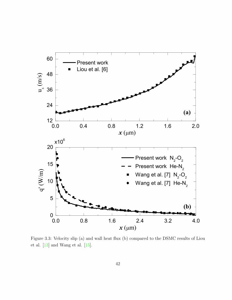
0.0 0.4 0.8 1.2 1.6 2.012

24

36

48

60

x ( m)

(a)

Present work Liou et al. [6]

x ( m)

0.0 0.8 1.6 2.4 3.2 4.00

5

10

15

20

u s (m

/s)

q' (W

/m)

Present work N2-O2

Present work He-N2

Wang et al. [7] N2-O2

Wang et al. [7] He-N2

(b)

x106

Figure 3.3: Velocity slip (a) and wall heat flux (b) compared to the DSMC results of Liou

et al. [13] and Wang et al. [15].

42

Table 3.2: Geometrical and operational specifications of different cases.

Mixture

H L m′′in Tw Mass

(µm) (µm) (kg/m2s) (K) % fraction

H2 N2 CO2

Case 1 H2/N2 1.5 6.0 50.0 350 10.0 90.0 −Case 2 H2/N2 1.5 6.0 50.0 300 10.0 90.0 −Case 3 H2/N2 1.5 6.0 100.0 350 10.0 90.0 −Case 4 H2/N2 1.5 6.0 50.0 400 10.0 90.0 −Case 5 H2/N2 4.0 16.0 50.0 350 10.0 90.0 −Case 6 H2/N2/CO2 1.5 6.0 50.0 350 2.7 37.8 59.5

rarefaction continuously goes up. The predictions of the two methods are very closer to

each other where non–equilibrium effects are less intense.

Figure 3.5 shows slip velocity data for Cases 1–4. Effect of the wall temperature Tw is

presented by Cases 1,2, and 4. As seen, slip velocity predicted by DSMC for isothermal

flow (Case 2) is a little higher. The reason can be the temperature gradient caused by

viscous dissipation which is naturally captured in DSMC and therefore, increases the slip

velocity. A good agreement is observed for Cases 1 and 4 in which the temperature gradient

produced by higher Tw increases the slip velocity. Cases 1 and 3 demonstrate the effect

of higher inlet mass flux m′′in. By elevating m′′in, velocity gradients and therefore, non–

equilibrium effects increase along the channel causing higher slip velocity. This rise in

the slip velocity is more pronounced at the outlet compared to the inlet since the outlet

pressure is kept constant and thus, the stream velocity and velocity gradients have much

larger values. As observed, DSMC and Navier-Stokes show some deviations for Case 3 due

to the intense non–equilibrium effect resulting from these gradients.

Distributions of axial (x–component) and normal (y–component) velocities across the

channel is shown in Figure 3.6 at three locations along the channel for Case 1. A very

good agreement is generally observed which implies that the viscosity of the gas mixture

is effectively simulated by DSMC. The largest different between the two methods happens

43

0 1 2 3 40.00

0.25

0.50

0.75

1.00

1.25

x/H

NSWS/J - Full NSWS/J - No Thermal Creep DSMC

u s/ur

H2/N2 Mixture

Figure 3.4: Slip velocity distribution along the channel obtained from Navier–Stokes and

DSMC methods. ur is the reference velocity (ur = 50m/s).

44

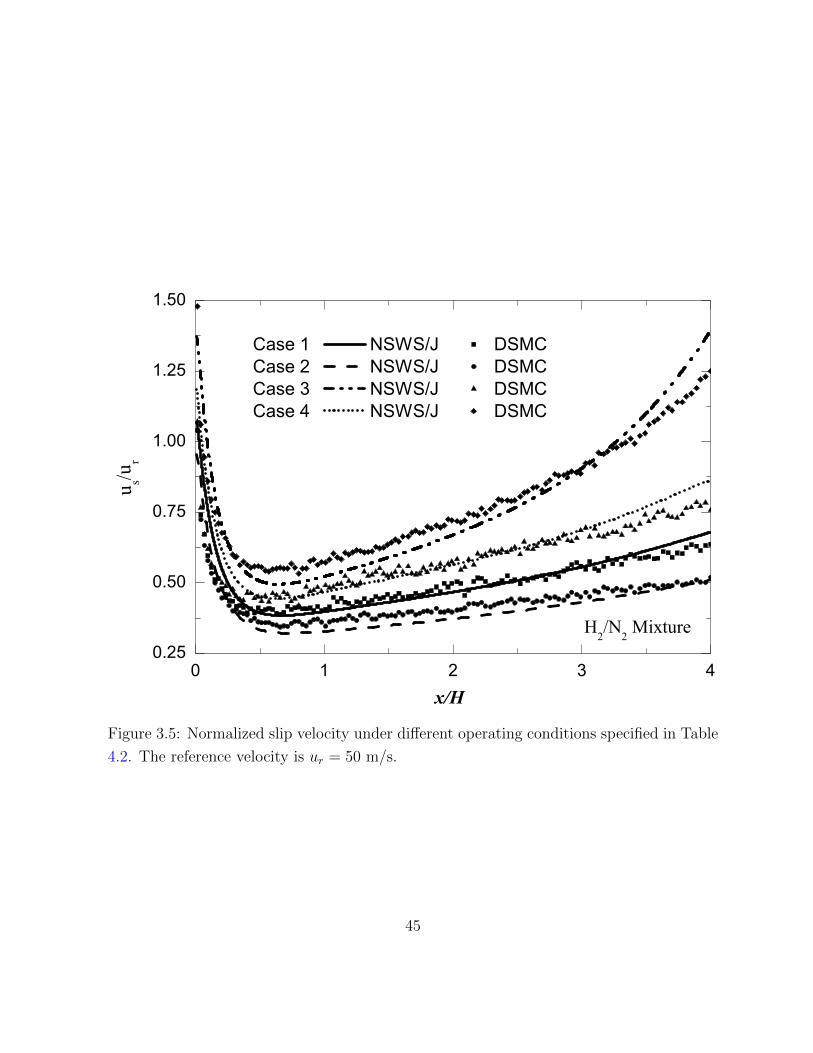
0 1 2 3 40.25

0.50

0.75

1.00

1.25

1.50

x/H

Case 1 NSWS/J DSMCCase 2 NSWS/J DSMCCase 3 NSWS/J DSMCCase 4 NSWS/J DSMC

u s/ur

H2/N2 Mixture

Figure 3.5: Normalized slip velocity under different operating conditions specified in Table

4.2. The reference velocity is ur = 50 m/s.

45

at the mid–plane and closer to the outlet. It seems that higher rarefaction effects at the

outlet (due to larger mean free path and Kn) penetrate upstream into the bulk motion

causing Navier-Stokes slip model to digress more from DSMC.

Effects of the channel height on slip velocity data of Cases 1 and 5 are demonstrated

in Figure 3.7. As seen, by rising the channel height and decreasing Kn, the slip velocity

decreases as expected. The two methods agree well for both cases; however, for the smaller

channel (and hence, higher non–equilibrium conditions) there is a little deviation at the

inlet. Variations of Kn2 is also shown for both Cases and demonstrates that the rarefaction

is more magnified at the outlet by decreasing the height. This occurs due to rapid pressure

drop close to the outlet causing steep Kn elevation which also causes a discrepancy between

the results.

Profiles of mass fraction Yi of H2 and N2 across the channel are shown in Figure 3.8 for

Case 1 at x/H=0.259. As mentioned before, H2 and N2 have large mass discrepancy and

this causes considerable difference in their diffusion. H2 is the lightest available molecules

and therefore its most probable thermal speed Vmp is very high according to the relation:

Vmp =√

2kT/m. This increases the diffusion of H2 upstream especially at the vicinity of

the wall where the gas temperature is higher. As seen in the magnified view of Figure 3.8,

this causes non–uniform variations for N2 mass fraction close to the wall. Moreover, YN2

decreases near the wall which proves higher upstream diffusion of H2 in this location. There

is almost a constant difference between predictions of the two methods with an amount of

less than 8% and 1% for H2 and N2, respectively. It should be noted that this deviation is

partly due to the difference in the method of enforcing constant mass flux at the entrance

for DSMC and Navier-Stokes. For DSMC the iterative nature of imposing constant m′′inmakes the obtained results to be between the specified values and the results of the previous

step. In addition, values of the stream velocity and the number density are adopted from

the boundary cell since these are not accessible at the boundary. Therefore, m′′in has small

differences (slightly lower) which is carried into the channel with the flow and is one of

the causes of the deviation seen in Figure 3.8. Furthermore, the upstream diffusion of

lighter species affects m′′in applied by the Navier-Stokes method, especially in the region

2Wall Knudsen number is calculated from the conventional definition of Knudsen number λ/H with

the mean free path λ obtained at the vicinity of the wall.

46

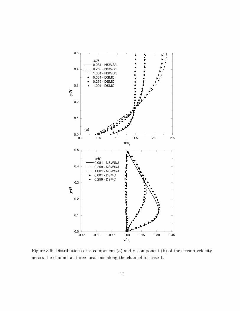
0.0 0.5 1.0 1.5 2.0 2.50.0

0.1

0.2

0.3

0.4

0.5

v/ur

(a)

x/H 0.081 - NSWS/J 0.259 - NSWS/J 1.001 - NSWS/J 0.081 - DSMC 0.259 - DSMC 1.001 - DSMC

u/ur

-0.45 -0.30 -0.15 0.00 0.15 0.30 0.450.0

0.1

0.2

0.3

0.4

0.5

y/H

y/H

x/H 0.081 - NSWS/J 0.259 - NSWS/J 1.001 - NSWS/J 0.081 - DSMC 0.259 - DSMC

Figure 3.6: Distributions of x–component (a) and y–component (b) of the stream velocity

across the channel at three locations along the channel for case 1.

47

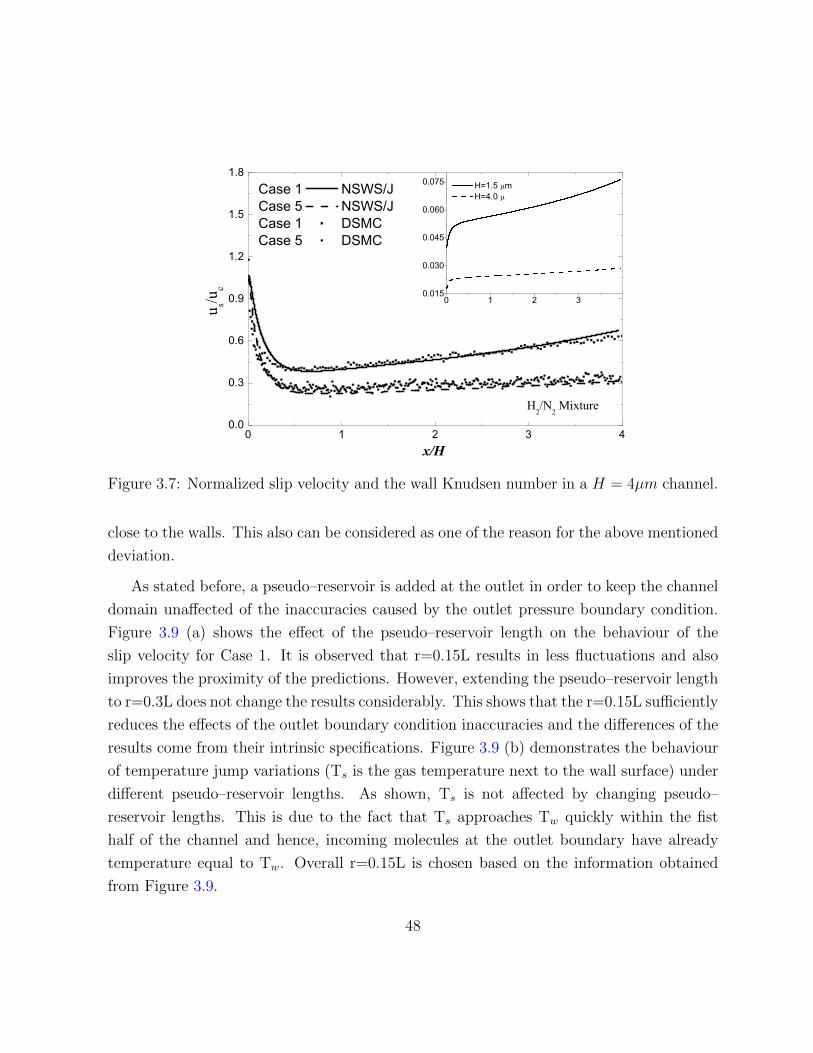
0 1 2 3 40.0

0.3

0.6

0.9

1.2

1.5

1.8

x/H

Case 1 NSWS/JCase 5 NSWS/J Case 1 DSMCCase 5 DSMC

u s/u

c

H2/N

2 Mixture

0 1 2 30.015

0.030

0.045

0.060

0.075 H=1.5 m H=4.0

Figure 3.7: Normalized slip velocity and the wall Knudsen number in a H = 4µm channel.

close to the walls. This also can be considered as one of the reason for the above mentioned

deviation.

As stated before, a pseudo–reservoir is added at the outlet in order to keep the channel

domain unaffected of the inaccuracies caused by the outlet pressure boundary condition.

Figure 3.9 (a) shows the effect of the pseudo–reservoir length on the behaviour of the

slip velocity for Case 1. It is observed that r=0.15L results in less fluctuations and also

improves the proximity of the predictions. However, extending the pseudo–reservoir length

to r=0.3L does not change the results considerably. This shows that the r=0.15L sufficiently

reduces the effects of the outlet boundary condition inaccuracies and the differences of the

results come from their intrinsic specifications. Figure 3.9 (b) demonstrates the behaviour

of temperature jump variations (Ts is the gas temperature next to the wall surface) under

different pseudo–reservoir lengths. As shown, Ts is not affected by changing pseudo–

reservoir lengths. This is due to the fact that Ts approaches Tw quickly within the fist

half of the channel and hence, incoming molecules at the outlet boundary have already

temperature equal to Tw. Overall r=0.15L is chosen based on the information obtained

from Figure 3.9.

48

0.0 0.1 0.2 0.3 0.4 0.5 0.6 0.7 0.8 0.9 1.00.0

0.1

0.2

0.3

0.4

0.5

Mass Fraction

YH2

NSWS/J DSMC

YN2

NSWS/J DSMC

y/H

H2/N

2 Mixture

0.897 0.900 0.903 0.906 0.909 0.912 0.9150.0

0.1

0.2

0.3

0.4

0.5

y/H

Figure 3.8: Hydrogen and nitrogen mass fractions across the channel at x/H = 0.259 for

case 1.

49

0 1 2 3 4

0.4

0.6

0.8

1.0

1.2

H2/N2 Mixture

x/H

(a)

NSWS/J DSMC r = 0 DSMC r = 0.15L DSMC r = 0.30L

x/H

H2/N2 Mixture

0 1 2 3 40

10

20

30

40

u s/u

rT w

-Ts

NSWS/J DSMC r = 0 DSMC r = 0.15L DSMC r = 0.30L

(b)

Figure 3.9: Velocity slip (a) and temperature jump (b) predictions for case 1 with different

pseudo–reservoir lengths. ur=50m/s

50

The results of the slip velocity for a multi–component gas flow of H2/N2/CO2 are shown

in Figure 3.10 (a). A behaviour similar to Figure 3.4 is seen and therefore, adding another

component to the flowing gas did not change the agreement of the two methods. The

discrepancies observed close to the inlet and outlet boundaries are analogous to Figure 3.4

and are caused by non–equilibrium effects. Figure 3.10 (b) shows mass fractions of the

three species. A good conformity between DSMC and Navier-Stokes methods is generally

observed. As shown in the magnified view, the mass fraction of H2 is higher close to the

wall. It was stated previously that this occurs due to higher upstream diffusion rate of H2

near the wall.

Heat transfer

Apart from the statistical scatter introduced naturally by the DSMC algorithm, the tem-

perature jump data for Cases 1,3, and 4 for both methods are in very good compliance as

shown in Figure 3.11. The temperature jump generally has its highest value at the inlet

due to larger velocity and temperature gradients and gradually fades out along the channel.

It is observed that the presence of a temperature gradient is essential for having tempera-

ture jump at the wall since, there is no temperature jump close to the outlet, despite the

equilibrium effects present there. That is also why the temperature jump distribution is

not affected by the outlet conditions (e.g. the length of the pseudo–reservoir).

The simulation results of the wall heat flux for Cases 1,3, and 4 are shown in Figure 3.12.

This quantity in the DSMC method is obtained from:

q′′ =

∑Ng

i=1 e∗i −

∑Ng

i=1 eiA ·∆t

(3.3)

where e∗i is the summation of translational and internal energies (total energy) of a single

simulating particle reflected back from the wall surface having the wall temperature (ther-

mally diffuse), ei is the total energy of the same simulating particle right before hitting the

surface, ∆t is the DSMC sampling time step and A is the surface area of the incident cell

and is equal to ∆x. As seen, predictions of the methods are in very good agreement. The

maximum deviation of 10% is observed for Case 4 at the inlet. The reason is mainly due

to intense non–equilibrium conditions close the the inlet which lead to a difference between

51

0 1 2 3 40.0

0.2

0.4

0.6

Mass Fraction

H2

H2/N

2/CO

2 Mixture

(a)

NSWS/J DSMC

x/H

H2/N

2/CO

2 Mixture

0.0 0.2 0.4 0.6 0.8 1.00.0

0.1

0.2

0.3

0.4

0.5

u s/ur

CO2N

2

y/H

(b)

0.020 0.024 0.0280.0

0.1

0.2

0.3

0.4y/H

H2 Mass Fraction

Figure 3.10: Velocity slip (a) and mass fractions of H2/N2/CO2 at x/H = 0.157 (b) for

the gas mixture of Case 6

52

0 1 2 3 40

5

10

15

20

25

30

x/H

NSWS/J DSMC Case 1 Case 1 Case 3 Case 3 Case 4 Case 4

T w-T

s (K)

H2/N

2 Mixture

Figure 3.11: Temperature discontinuity at the edge of the Knudsen layer under different

operating conditions.

53

0.0 0.5 1.0 1.5 2.00.0

5.0x106

1.0x107

1.5x107

2.0x107

2.5x107

3.0x107

3.5x107

W

all h

eat f

lux

q' (W

/m)

x/H

Case 1 NSWS/J DSMCCase 3 NSWS/J DSMCCase 4 NSWS/J DSMC

H2/N2 Mixture

Figure 3.12: Wall heat flux along the channel under different operating conditions; The

results of Case 1 are multiplied by 0.5 to avoid cluttering.

the mean collision rate of molecules with the wall calculated by DSMC and Navier–Stokes

methods. In Navier-Stokes this quantity is calculated by the Maxwell distribution in the

form of continuum relations which is necessarily applicable just for the equilibrium state.

Whereas, in DSMC the mean collision rate is sampled directly. Therefore, heat flux values

obtained from the DSMC are slightly lower than Navier-Stokes since in rarefied conditions

less molecules are expected to hit the wall surface. This results in less energy carries into

the flow as shown in Figure 3.12.

54

3.2.4 Summary

The results of DSMC and Navier-Stokes methods are compared for binary and multi–

component gas mixture micro–flow in the slip regime. The Navier-Stokes results are ob-

tained from a verified code with slip/jump boundary treatment developed by Qazi Zade

et. al. [45]. The gas mixtures used in this study were N2/H2 and N2/H2/CO2. This

combination ensures to challenge the ability of DSMC in reproducing flow properties such

as viscosity and molecular diffusion for a mixture with large mass discrepancies and multi–

atomic molecules. A constant mass flux is imposed at the inlet and an atmospheric pressure

is applied at the outlet. In order to prevent the channel domain from being affected by the

inaccuracies resulting from the Maxwell distribution used in the outlet pressure boundary

condition, a pseudo–reservoir with specular reflection on its walls is added at the channel

exit. It is found that the pseudo–reservoir is enough to be 15% of the channel length.

Based on the considered cases, effects of the channel height, the wall temperature and the

inlet mass flux on the conformity of the methods on prediction of the slip velocity, the

temperature jump, the wall heat flux, and velocity profiles are studied. It was found that

the VSS collision method should be used for capturing near wall phenomena correctly.

3.3 Effect of higher order pressure boundary condi-

tions

AS stated before, numerical simulation of multi-species gas flows through micro/nano-

channels is the first step for modelling chemically reacting flows. One of the challenges on

the way of modelling such flows using DSMC is the implementation of the flow boundary

conditions. A prescribed pressure is the most commonly used inlet/outlet boundary condi-

tion. In order to control the pressure value at the boundary, local values of stream velocity

components, density and temperature must be either known or calculated in each time

step. The temperature and the number density are imposed directly at the inlet boundary

as their values are known. For the outlet boundary, these quantities are taken from the

sampled values of adjacent cells. Two different methods for evaluating velocity components

55

have been reported for the case of single-species gas flows. The first method, introduced

by Nance et al. [46], uses the characteristic line equations of sound wave propagation

for the outlet boundaries and Wang and Li [14] further developed it for inlet boundaries.

One of the fundamental assumptions of the characteristic line method is that the flow is

isentropic. Our previous simulations Qazi Zade et al. [45], in agreement with Fang et

al. [13], show that this assumption causes non-physical behavior in non-adiabatic flows

as expected. The second method of obtaining unknown flow variables at the boundary

involves using the velocity field information from the previous iteration step and applying

a mass balance scheme at the boundary. Ikegawa and Kobayashi [11] first introduced this

method using the number of molecules crossing the boundary during the last time step.

However, the values of the molecular flux calculated during one time step are so small that

the pressure boundary condition becomes unstable. Wu and Tseng [47] solved this problem

by employing ensemble average values of flow properties, taken over previous time steps,

in evaluating the molecular flux. This method has no extra assumptions and is based on

the conservation of mass. Using values of the density, the temperature and velocity com-

ponents calculated from either of the above described methods, the molecular flux at the

boundary is calculated via a relation derived from the Maxwell velocity distribution.

For multi-component flows, species concentrations should also be evaluated at the out-

let boundary. As of yet, there is no specific methodology proposed in the literature, and

available studies try to circumvent the need for calculating the species concentrations. Yan

and Farouk [17] analyzed the mixing process of a binary gas flow and used the outlet bou-

ndary without any special treatment, i.e., those molecules leaving the domain were simply

removed. Wang and Li [48] studied the mixing efficiency of N2 and CO in a parallel micro-

mixer, exerting a constant pressure both at the inlet and the outlet boundaries. However,

the molecular specifications of both selected species were very similar, and therefore, the

effect of mass diffusion was reasonably negligible and the utilization of the single-species

boundary treatment was possible. Wang et al. [15] also simulated binary gas mixture

micro-flows with different gas compositions between parallel plates in order to verify their

new constant heat flux boundary condition. The details of the pressure boundary con-

ditions they implemented were not described, but based on our simulations, the pressure

ratio of 3.0 applied to a 1µm × 4µm micro-channel results in a near sonic velocity at the

56

outlet. Under such a condition, the exit pressure cannot practically be controlled since

the number of molecules entering the domain at the boundary is negligible. In the present

work, a pressure boundary condition for a multi-species flow is introduced based on the Wu

and Tseng [47] methodology. The number density for each species is sampled separately

and species concentrations are calculated accordingly. The results for high speed flows are

verified against Wang et al. [15] results. However, the accuracy of the method in predict-

ing species concentrations decreases considerably as the flow speed is reduced. In an effort

to overcome this problem, we noticed the effects of the rarefaction caused by the rapid

pressure drop near the outlet flow boundary. This introduces non-equilibrium conditions

and hence put the applicability of the commonly used Maxwell velocity distribution into

question. The Maxwell distribution function is the first term of the general distribution

function f written in a perturbation series as [1]:

f = f 0 + f 1 + f 2 + ... (3.4)

where f 0 is the solution of the Boltzmann equation for a homogeneous simple gas in

an equilibrium condition. By considering f 1 in the determination of f , deviations from

equilibrium are taken into account up to first order. f 1 is obtained by the Chapman-Ens-

kog solution of the Boltzmann equation. Here, the proposed pressure boundary condition

for multi-species gas micro-flows is explained in detail and then modified by the Chapman-

Enskog velocity distribution. The molecular flux expression is also modified accordingly

and its general explicit form is presented. Then, the effect of the first order variations on

controlling boundary pressure are demonstrated.

It should be noted that f 1 is derived by perturbing the distribution function f by a small

amount from equilibrium conditions, and therefore, the accuracy of this method decreases

as Kn increases. Nevertheless, the Chapman-Enskog distribution offers higher accuracy

in comparison to the commonly used Maxwell distribution which neglects non-equilibrium

effects.

57

3.3.1 Inlet and outlet boundary conditions

General description

As stated before, a specified constant pressure condition is commonly used at the in-

let/outlet flow boundaries. In DSMC, the pressure is controlled by adjusting the velocity

and the density of the gas which enters the domain at the boundary. The density of each

species is calculated by the ideal gas law, pj = njkT , where, pj and nj are the partial

pressure and number density of the species j, respectively. In the boundary treatment pro-

posed here, the temperature T is set equal to the corresponding value of the cell adjacent

to the boundary, and the partial pressure of each species is calculated from pj = Xjp in

which, Xj = nj/n0 is the mole fraction evaluated in the adjacent cell and p is the pressure

to be imposed at the boundary. Having the value of nj, the velocity component normal

to the boundary for each species, uj, is then calculated by a mass conservation scheme as

follows:

njuj = N+j − N−j (3.5)

where the values of N+j and N−j are the number fluxes of species j which cross the boun-

dary in the positive and negative directions, respectively. At a boundary, either N+j or N−j

which tends to leave the domain is known and can be evaluated by a sampling process,

but the other one which is directed into the domain is not known and is obtained from:

N+/−j = nj

∞∫−∞

∞∫−∞

∞/0∫0/−∞

ujfj dujdvjdwj (3.6)

where, u, v and w are velocity components, each of which is composed of a mass averaged

stream part, u0, v0 and w0, and a peculiar part, u′, v′ and w′, i.e., u = u0 + u′, v = v0 + v′

and w = w0 + w′. In the above equation, it is assumed, without any loss of generality,

that the vector normal to the boundary is parallel to the x-coordinate (Figure 3.13), thus,

the velocity component uj is normal to the flow boundary. In addition, f is the veloc-

ity distribution function which is given by the Maxwell distribution function, f 0, in the

conventional DSMC as [1]:

f (0) = V −3mp π

−3/2 exp(−v′2/V 2

mp

)(3.7)

58

Figure 3.13: The schematic of the channel under study

where ~v′ = (u′, v′, w′) and Vmp is the most probable velocity of the molecules. The result

of the integration in Equation (3.6) using f 0 instead of f is [1]:

N(0)+/−j =

njSnVmpj2√π

(exp

(−s2

j

)±√πsj (1± erf (sj))

)(3.8)

where, sj is defined as sj = u0/Vmpj and u0 is calculated from u0 =∑

j Yjuj where Yj =

ρj/ρ0. Thus, the number of molecules that enter the boundary cell face with area A at the

current time step ∆t is obtained from N(0)j = N

(0)j A∆t. Velocities of the entering molecules

are assigned based on an acceptance-rejection method [1]. Those particles which leave the

flow domain are removed and the number of molecules inside the domain is corrected

correspondingly.

The proposed constant pressure boundary condition must predict the flux of particles

accurately for each participating component entering the domain with regard to the im-

posed pressure. As it will be shown in the results, for low velocity flows, this method

overestimates the molecular flux at the outlet, especially near the walls. In order to study

the effect of non-equilibrium conditions near the walls on the prediction of molecular num-

ber flux, the second order approximation of the velocity distribution is used by considering

the second term of Equation (3.4). According to the Chapman-Enskog solution, the second

order approximation of f can be represented as a small perturbation from equilibrium state

59

( f 0) in the form:

f = f 0 + f 1 = f 0(1 + Φ) (3.9)

By substituting the second approximation of f into the Boltzmann equation and performing

some nontrivial mathematical operations (details can be found in [28]), the general form

of Φ for a binary gas mixture is obtained as:

Φ1 = −A1· ~∇(ln(T ))−D1· ~d12 − 2B1 : ~∇~v0

Φ2 = −A2· ~∇(ln(T ))−D2· ~d12 − 2B2 : ~∇~v0

(3.10)

in which, subscripts 1 and 2 belong to the species and the vector ~d12 is given as:

~d12 = ~∇X1 +

(X1

ρ2

ρ0

−X2ρ1

ρ0

)~∇ln(p) (3.11)

The vectors A and D and the tensor B given in Equation (3.10) are of the forms ~A =

~v′A(v′), ~D = ~v′D(v′) and B =˚−→v′−→v′B(v′)1, where B, A and D were derived independently

by Chapman and Enskog and can be found in [28]. An organized list of the equations

and required steps to evaluate the function B and then functions A and D for binary gas

mixtures are presented in Appendix A following the method of Tipton et al. in [49, 50].

The number flux expression using the Chapman-Enskog distribution

In order to incorporate the effect of flow variable gradients in determining the number flux

of molecules, Equation (3.9), is used in Equation (3.6) which gives:

N(1)+/−j = N

(0)+/−j −

∞∫−∞

∞∫−∞

∞/0∫0/−∞

2Bj + Aj +Dj × f (0)j uj dujdvjdwj (3.12)

where Bj contains the effect of velocity gradients and viscosity, Aj contains effects of

temperature gradients and thermal diffusion, and Dj includes effects of pressure and spe-

cies concentration gradients and molecular diffusion. The integration process reported in

1W = W − 13 (Σwii) δ where δ is the unity tensor

60

the literature is focused on calculating the number flux of particles crossing the Knudsen

layer formed on the walls where the stream part of uj, which is normal to the wall is set

equal to zero [51, 52]. To extend the integration results to a flow boundary (inlet/outlet),

general expressions for Bj, Aj and Dj functions are represented as follows based on the

relations in [49, 50]:

B1 = b1˚−→C 1−→C 1: ~∇~v∗01

B2 = b−1˚−→C 2

−→C 2: ~∇~v∗02

(3.13)

A1 =a1

(52− C2

1

)+ kT

d0M

1/21

ρ2ρ0

+ d1

(52− C2

1

)~C1· ~∇ln(T )

A2 =a−1

(52− C2

2

)+ kT

−d0M

1/22

ρ1ρ0

+ d−1

(52− C2

2

)~C2· ~∇ln(T )

(3.14)

D1 =d0M

1/21

ρ2ρ0

+ d1

(52− C2

1

)~C1· ~d12

D2 =−d0M

1/22

ρ1ρ0

+ d−1

(52− C2

2

)~C2· ~d12

(3.15)

where kT is the thermal diffusion coefficient, ~Cj = ~v′j/Vmpj and ~v∗0j = ~v0/Vmpj. The

integration of functions Aj, Dj and Bj, shown on the right hand side of Equation (3.12),

are labelled as BN+/−j , AN

+/−j and DN

+/−j for clarity. These integrations give the following

results:

BN+/−1 = ±

n1b1V2mp1

6√π

2∂u∗01∂x− ∂v∗01

∂y− ∂w∗01

∂z

exp(−u∗201)

BN+/−2 = ±

n2b−1V2mp2

6√π

2∂u∗02∂x− ∂v∗02

∂y− ∂w∗02

∂z

exp(−u∗202)

(3.16)

AN+/−1 = ±n1Vmp1

4√π

u∗01 (d1kT + a1) exp(−u∗201)

+√πd0kT

√M1

ρ2

ρ0

erf(u∗01)± 1∂ln(T )

∂x

AN+/−2 = ±n2Vmp2

4√π

u∗02 (d−1kT + a−1) exp(−u∗202)

−√πd0kT

√M2

ρ1

ρ0

erf(u∗02)± 1∂ln(T )

∂x

(3.17)

61

DN+/−1 = ±n1Vmp1

4√π

d1u

∗01 exp(−u∗201) +

√πd0

√M1

ρ2ρ0erf(u∗01)± 1

×(

X1ρ2ρ0−X2

ρ1ρ0

)∂ln(p)∂x

+ ∂X1∂x

DN

+/−2 = ±n2Vmp2

4√π

d−1u

∗02 exp(−u∗202)−

√πd0

√M2

ρ1ρ0erf(u∗02)± 1

×(X1

ρ2ρ0−X2

ρ1ρ0

)∂lnp∂x

+ ∂X1∂x

(3.18)

The final value of molecular number flux derived from the Chapman-Enskog velocity dis-

tribution is then calculated from:

N(1)+/−j = N

(0)+/−j −

BN

+/−j + AN

+/−j + DN

+/−j

(3.19)

The calculated value of N(1)+/−j is next substituted into Equation (3.5) and the procedure

described following that equation is applied to improve the pressure boundary condition

for the DSMC method. Accordingly, equations used in the pressure boundary condition

derived from the Maxwell (DSMC/M) and the Chapman-Enskog (DSMC/CE) distribution

functions are as follows:

DSMC/M: Equation (3.5) with Equation (3.8)

DSMC/CE: Equation (3.5) with Equation (3.19)

Above mentioned acronyms are used for the rest of the discussions.

3.3.2 Numerical verification

The DSMC code for this study was prepared based on the algorithm proposed by Bird [1].

The modules were updated and modified for simulating flows of multi-species gas mixtures

in two-dimensional channels. A schematic of the solution domain is shown in Figure 3.13.

For verification purposes, the geometry of the domain for this study was selected the same

as Wang et al. [15], with L = 4µm and h = 1µm. This domain was partitioned into 140×60

structured rectangular cells. A gas mixture of He-N2 with a molar concentration of 50%-

50% flows inside this channel with the flow parameters stated in Case 1 of Table 3.3. At

62

Table 3.3: Operational parameters of different simulation cases. For all cases, the mixture

is 50%-50% by molecular number density, Tw=350K and Tin=300K.

pin pout Knin Knout Rein

(bar) (bar)

Case 1 3.0 1.0 0.029 0.081 16.5

Case 2 1.0 0.5 0.090 0.199 3.1

Case 3 1.2 1.0 0.079 0.101 0.4

Case 4 0.6 0.5 0.158 0.211 0.2

the first step, velocity, temperature, heat transfer and pressure results obtained from both

DSMC/M and DSMC/CE were compared to Wang et al. [15], as shown in Figures 3.14-

3.15 respectively. An excellent agreement is observed for all flow properties investigated.

Results of the present code for gas mixture slip flows (Kn <0.1) have also been verified in

detail against Navier-Stokes simulations and reported in Qazi Zade et al. [45], which will

not be repeated here.

3.3.3 Results and discussion

As indicated in Section 3.3.1, calculating N+ and N− is the first step for applying the

DSMC pressure boundary condition. Since the stream velocity is in the positive direction,

N+ has a much greater value than N− and therefore, using a higher order distribution

is more critical for calculating N−. Hence, the rest of the discussion is focused on N−

which is used for implementing the outlet pressure boundary condition. It is observed

in Figures 3.14-3.15 that adopting the Chapman-Enskog distribution for Case 1 does not

affect the temperature and velocity fields. The reason lies in the high pressure ratio of this

case which leads to a high velocity at the channel outlet. This means that the number

flux of molecules leaving the domain (the value of N+ in Equation (3.5)) is so high that

the outlet velocity is almost unaffected by the number flux of molecules diffusing upstream

63

u (

m/s

)

0

50

100

150

200

250

T (

K)

290

300

310

320

330

340

350

y/h

0 0.1 0.2 0.3 0.4 0.5

Figure 3.14: Verification of velocity and temperature cross-sectional profiles for Case 1

against Wang et al. [15] reported at x/Lc = 0.1 (”” from Maxwell, ”∗” from Chap-

man-Enskog and continuous line [15]) and x/Lc = 0.7 (”M” from Maxwell, ”×” from

Chapman-Enskog and dash line [15]).

(the value of N− calculated from Equation (3.19)) at the boundary. Applying a high

temperature at the walls has the same effect since the resulting gas expansion produces

a high stream velocity at the outlet. Decreasing the pressure ratio will increase the value

of N− and thus magnify the role of the boundary condition. Generally, the influence of a

pressure boundary condition on a flow depends on Kn and the stream velocity (or pr). In

order to study their effects, four different cases are considered here as listed in Table 3.3:

Case 1 deals with high stream velocity (pr=3.0) and low Kn; Case 2 deals with high stream

velocity (pr=2.0) and high Kn; Case 3 deals with low stream velocity (pr=1.2) and low Kn;

and Case 4 deals with low stream velocity (pr=1.2) and high Kn. The Kn range of these

64

q w(×

106 W/m

2 )

−20

−15

−10

−5

0

x/L

0 0.2 0.4 0.6 0.8 1

N2-O2 MaxwellN2-O211

He-N2 MaxwellHe-N211

He-N2 Chapman-Enskog

(a)

P/P o

ut

1

1.5

2

2.5

3

x/h

0 1 2 3 4

Pr=3.0 (DSMC/M)Pr=3.0 (DSMC/CE)Wang et al.11

(b)

Figure 3.15: Comparison of (a) wall heat flux and (b) pressure distribution obtained from

DSMC/M and DSMC/CE for Case 1 with Wang et al. [15] (negative heat flux represents

heat being extracted from the wall).

65

cases covers the slip and the initial part of the transition regimes which are practically more

important. The authors could not find any experimental data with the same or similar

properties as Cases 2-4 in the available literature for verification purposes. An option is

verification against DSMC results which are obtained from a full order velocity distribution

used in the applied pressure boundary condition. For this purpose, a channel with the same

hight but a length Lext greater than Lc = 4.0µm was simulated and the results of the first

4.0µm of the channel are considered as the desired data, here forth called the “reference

data”. This way, the velocity distribution and hence N− are naturally evaluated by DSMC

itself across the channel at 4.0µm, and therefore, have a full order accuracy. In order to

keep the pressure distribution throughout the first 4.0µm of the channel the same as the

case under study, the pressure at 4.0µm was kept at the corresponding value by imposing

an appropriately lower pressure at the outlet. This was achieved by correcting an initial

guess for the outlet pressure as the simulation marched to steady state conditions. It

should be noted that the outlet pressure is imposed by either DSMC/M or DSMC/CE.

Therefore, possible inaccuracies present in the evaluation of N− can affect reference results

by upstream diffusion. To prevent this, the extended channel is lengthened and hence the

pressure ratio and the outlet velocity are increased. As discussed earlier for Case 1, if the

outlet velocity is high enough (adequately long channel) the value of N− is negligible.

In order to determine whether the velocity distribution function affects the evaluation of

N−, the difference between the values of N− crossing the vertical face of the cells adjacent

to the walls obtained from DSMC and the Maxwell distribution are shown in Figure 3.16 for

Case 2 as an example. The values corresponding to DSMC were obtained by direct sampling

of the number of molecules crossing the cell face. For calculating N− values from the

Maxwell distribution (zero line) equations of DSMC/M and flow properties from the DSMC

simulation were used. As expected, the DSMC results deviate from equilibrium conditions

with the maximum departure around 8% near the outlet. This deviation suggests that a

velocity distribution with a higher order than the Maxwell distribution (which is used in the

conventional pressure boundary condition, DSMC/M) is required to calculate the molecular

flux accurately. As will be shown, this is especially necessary in a correct implementation

of a constant pressure boundary condition for gas mixtures. Figure 3.16 also shows that

non-equilibrium effects are higher near the outlet which is due to higher rarefaction effects

66

(0)-

x/h

Figure 3.16: Variations of ∆N = N−DSMC − N (0)− relative to N (0)− along the channel for

Case 2; N−DSMC is the number flux calculated by DSMC and N (0) the one calculated from

DSMC/M crossing the vertical face of the cells adjacent to the walls.

present there in this flow. This fact is clearly seen in Figure 3.17 in which Kn continuously

increases along the channel. These non-equilibrium effects are taken into account by first

order using the Chapman-Enskog velocity distribution (DSMC/CE), which should result in

a behavior closer to the DSMC reference solution. Figure 3.17 also shows that simulation

results are insensitive to DSMC/M or DSMC/CE for the high speed conditions of Case 1

and Case 2.

Figure 3.18 presents the contour plots of the He concentration in a gas mixture of

He-N2 for Case 2 obtained from DSMC/M and DSMC/CE. As shown, the concentration

distribution is almost the same for both methods. A notable point is an accumulation

of N2 between the middle and the outlet of the channel. This behaviour can either be a

physical phenomenon or produced by inaccuracies in calculating N− using DSMC/M or

67

Figure 3.17: Pressure and Kn distributions for higher speed cases, i.e. Case 1 and Case 2;

(M) and (C) represent the results of DSMC/M and DSMC/CE respectively.

DSMC/CE. In order to resolve this, the results are compared to the “reference data” as

indicated before.

Concentration results of simulating two extended channels with Lext of 5.0µm and

6.0µm (Lc+h and Lc+2h respectively) are presented in Figure 3.19. In both cases, the

pressure at 4.0µm is kept at 0.5bar as described earlier. A N2 accumulation zone similar

to the one seen in Figure 3.18 still exists in 5.0µm long channel of Figure 3.19(a); however,

it has moved to a location beyond 4.0µm. In addition, this accumulation zone vanished

completely in the 6.0µm channel of Figure 3.19(b). This shows that such accumulation

was a result of inaccuracies in the calculation of N− used in the outlet pressure boundary

condition. It is worth noting that the pressure distributions in the first 4.0µm of both

channels shown in Figure 3.19 are the same. Our further studies revealed that the value

68

Figure 3.18: The contour plot of the number density of He in gas mixture flow of He-N2

for Case 2; thicker line: DSMC/M and thinner line: DSMC/CE

of N−j is underestimated for the species with heavier molecules. Furthermore, the pressure

ratio at which such behaviour emerges, depends directly on the molecular masses of the

species in the gas mixture (pr ≈2.5 for He-N2 and pr ≈1.5 for N2-O2). The 6.0µm channel

of Figures 3.19(b) is long enough that the high velocity produced at the outlet minimizes

the effect of N−j as discussed earlier in this section. Therefore, results of the first 4.0µm of

this case is used as the reference solution (DSMC/R) for the rest of the present study.

Contour plots of the He concentration for the low velocity cases, i.e., Case 3 and Case

4, are presented in Figure 3.20(a) and Figure 3.20(b) respectively. In this figure, the results

of DSMC/M and DSMC/CE (shown in the lower half of the channel) and the reference

data (shown in the upper half of the channel) are compared to each other. As shown, the

concentration is predicted almost the same using DSMC/M and DSMC/CE for lower Kn,

i.e., Case 3. For higher Kn, Case 4, however, results of the two methods considerably

deviate from each other both at the inlet and the outlet and DSMC/M fails to follow the

reference data. The trend of DSMC/CE results are closer to the reference and as well, it is

more accurate. The effectiveness of using DSMC/CE for high Kn and low velocity flows is

also seen in Figure 3.21. This figure shows pressure and Kn changes along the mid-plane

of the channel for lower speed cases. For Case 3 with lower Kn, DSMC/M and DSMC/CE

69

(a)

(b)

Figure 3.19: Contour plots of the He concentration for two extended channels with different

Lext of (a) 5.0µm and (b) 6.0µm and properties of Case 2.

70

(a)

(b)

Figure 3.20: Contour plots of the He concentration calculated from DSMC/M (thinner

lines, lower half), DSMC/CE (thicker lines, lower half), and the reference data (upper

half) for (a) Case 3 and (b) Case 4.

71

Kn

X (μm)

2

3

2

3

2

3

(a)

62

Kn

0.22

X (μm)

(b)

Figure 3.21: Variations of pressure and Kn along the mid-plane of the channel for lower

speed cases, i.e. (a) Case 3 and (b) Case 4.

72

simulations are almost the same, but DSMC/CE results for Kn are closer to the reference

data near the outlet. However, as shown in Figure 3.21(b), DSMC/M digresses considerably

from the reference results at higher Kn (Case 4) starting early in the channel. On the other

hand, using DSMC/CE results in almost exact Kn predictions. This observation that both

DSMC/CE and DSMC/M calculate the pressure distribution accurately conveys the fact

that number of molecules entering the channel at the outlet boundary is predicted well

by both methods; however, the composition of these molecules for participating species is

only calculated correctly by the higher order method, DSMC/CE, and that is why only

DSMC/CE is successful in simulating Kn accurately. This is fully consistent with the

results shown in Figure 3.20.

So far it is determined that adopting DSMC/CE works for low velocity and high Kn

flows; however, it can improve the results of high velocity or low Kn cases as well. Fig-

ure 3.22(a) shows that the slip velocity calculated by both DSMC/CE and DSMC/M

deviate from the reference solution near the outlet; however, applying DSMC/CE results

in closer behaviour to the reference data compared to DSMC/M. As expected, employing

the Chapman-Enskog distribution leads to partial improvements. It is worth noting that

a similar behavior has been observed in single component gas flows modelled with the

Maxwell pressure boundary condition [13, 53]. This supports the idea of the current study

that the velocity distribution function plays an important role in implementing pressure

boundary conditions.

Similarly, pressure values obtained from DSMC/CE are closer to the reference solution

for Case 2 (Figure 3.22(b)). As shown, the results obtained from both distributions are

essentially the same for the rest of the channel and agree well with the reference data.

Another observation from Figure 3.22(a) is the initial unexpected drop in the slip

velocity right after the inlet before it begins to increase with increasing Kn along the

channel. This behaviour, which is present in isothermal flows as well, is magnified as the

inlet Kn increases. It is in fact a numerical artifact caused by the uniform pressure enforced

at the inlet. As mentioned before, uniform pressure is the most practical inlet/outlet

boundary condition for DSMC in the absence of reservoirs. However, a perfectly uniform

pressure across the channel cross-section is not physically justified especially close to the

walls. Therefore, enforcing such a condition at the inlet results in an entrance adjustment

73

X (μm)

(a)

X (μm)

(b)

Figure 3.22: Velocity slip (a) and pressure variations (b) along the channel wall for

Case 2 based on the Maxwell distribution (DSMC/M), the Chapman-Enskog distribu-

tion(DSMC/CE), and the reference data (DSMC/R).

74

zone, where pressure and velocity distributions transform into their physical form. A

solution suggested by Roohi et al. [38] is to consider 10% of the channel as an entrance

region with specular molecular reflection at the walls. This increases the statistical scatter

in the results as well as the computation time, and therefore, not followed in this study.

Similar slip velocity drops close to the inlet have also been reported by Wang and Li [14]

and Fang and Liou [13].

For further understanding of the velocity distribution effects on calculating the molec-

ular number flux, a comparison was made similar to the one in Figure 3.16, including the

number flux obtained directly from DSMC/CE, as shown in Figure 3.23. For Case 2, as

seen in Figure 3.23(a), the Chapman-Enskog distribution results follow the same trend of

DSMC and can accurately replicate the DSMC number flux results in the entrance re-

gion where rarefaction effects are comparatively lower. The results from the two methods,

however, depart from each other along the channel with the maximum difference near the

outlet, and this difference is higher for He molecules. Figure 3.23(b) shows the same com-

parison for Case 4. It can be seen that DSMC/CE produces a more accurate distribution

for He in comparison to Case 2. This figure shows that DSMC/CE results for N2 are

higher than DSMC and generally mean values of the difference between DSMC/CE and

DSMC results is less that one third of the corresponding values for Case 2. This explains

why DSMC/CE results are closer to the reference data (see Figures 3.20 and 3.21). From

Figure 3.23, it is also clear that the value of N−j for He, calculated from DSMC/CE or

DSMC for Case 2 is lower than the DSMC/M results and that is why the value of N−jis overestimated for He in Figure 3.18. Similar results have been achieved for H2 in a

gas mixture of O2-H2. These observations again suggest that for the species with heavier

molecules, a velocity distribution of higher order than the Chapman-Enskog is required in

order to match the distribution naturally produced by DSMC. Due to the complexity and

the numerical effort required for the implementation of even the first order correction, a

utilization of higher order terms seems not feasible. Furthermore, higher order distribution

functions will not necessarily give the desired results for the conditions of Case 2.

75

3

x/h

4

(a)

2

x/h

4

2223

(b)

Figure 3.23: The variation of ∆N = N−− N (0)− relative to N (0)− along the channel for (a)

Case 2 and (b) Case 4; N (0)− is the number flux calculated from the Maxwell (DSMC/M)

distribution. 76

3.3.4 Summary

First, a pressure boundary condition has been proposed for the DSMC method in order

to simulate multi–species gaseous micro–flows. This pressure boundary condition was

implemented in the DSMC code previously verified against Navier–Stokes. The results

were also compared to other available DSMC results reported in the literature. Next,

the accuracy of the proposed pressure boundary condition was improved by adopting the

Chapman–Enskog distribution. Some cases with different Re and Kn ranges were studied

using the new boundary condition, and the results revealed that the velocity distribution

plays an important role in accuracy of the calculations at flow boundaries. In addition,

it was found that the molar fraction data obtained from the new boundary condition are

more accurate for low velocity and high Knudsen number (Kn) flows.

77

Chapter 4

Heterogeneous catalytic reacting

flows in transition regime

In this section, the intention is twofold: (1) to develop a numerical model applicable for

coupling surface chemical reactions and the flow field for highly rarefied flows (transition

flows) based on DSMC capabilities, and (2) to study the effects of geometrical and flow

specifications on the behaviour of catalytic reactions and as well on the flow variables.

The method used here is specially developed to couple the stochastic nature of DSMC

outputs with the conventional surface catalytic reaction analysis for steady-state conditions

and is described in Section 4.1. The resulting method is first used to simulate a flow of a lean

H2/Air flow in a parallel channel with platinum coated walls, and the results are compared

to those obtained from Navier-Stokes equations with slip-jump boundary conditions. Next,

the effects of different geometrical and boundary specifications are investigated using the

verified code.

4.1 Modelling surface catalytic chemical reactions

Heterogeneous chemical reactions take place on the catalytic walls of the channel. In

the present work, chemical reactions on the walls are modeled using a standard produc-

78

tion/consumption ODE system. This provides the flexibility of using available mechanisms

and taking advantage of DSMC. The general form of a production/consumption ODE is:

dθidt

= Σkjθmθn + rads,i − rdes,i (4.1)

where Σkjθmθn is the summation of Arrhenius reaction rates over all the sub–reactions

which participate in production/consumption of the species “i”. Thus, the range of “j” can

vary for different species. rads,i and rdes,i are adsorption and desorption rates respectively.

The number of ODEs for a chemical reaction is equal to the number of species involved in

the reaction, making an ODE system for an available reaction mechanism. Such an ODE

system has mostly stiff characteristics and requires a special solver in which the variable

time step method is utilized. The adsorption and desorption terms in Equation (4.1)

are responsible for exchanging molecules between the surface and the gas. These terms

are treated differently in the method introduced in this work to comply with the DSMC

algorithm. In general, the adsorption term for species i has the form:

rads,i = Kads,i (XPt∗)m (4.2)

where, rads is the rate of adsorption (mol/m2·s), X is the molar concentration on the

surface (mol/m2), subscript Pt∗ denotes the free platinum catalytic sites, superscript m is

the stoichiometric coefficient of the surface species, and Kads is the Arrhenius equivalent

rate constant which is of the form [54]:

Kads,k =γkΓm

Fk (4.3)

where, γk is the sticking coefficient of the species k, Γ is the density of total catalytic

surface sites (mol/m2) and Fk is the Mean Collision Rate (MCR) of the species k with

a unit area of the catalytic surface (mol/m2·s). Equations (4.2) and (4.3) imply that

a molecule hitting the surface is adsorbed with two probabilities: the sticking factor,

γk, which is the probability of being adsorbed if the molecule hits a free site, and the

probability of hitting a free site calculated from (XPt∗/Γ)m. In the continuum methods,

Fk is calculated by a relation derived from the Maxwell distribution. Some correction

coefficients are also applied to account for non-equilibrium effects on the surface due to

adsorption. In the DSMC method, however, Fk is directly sampled for each boundary cell

79

Figure 4.1: Different states of molecular collisions with the wall. This figure shows four

particles initially located in two boundary cells and hitting a surrounding wall. If the

collision is sampled based on initial position, particles 1 and 2 are considered to hit the

wall inside cell ”a” and as well particles 3 and 4 for will be considered for cell ”b”. However,

if the collision is sampled based on the collision spot on the surface, particles 1 and 3 will

be sampled for cell ”a” and particles 2 and 4 are sampled for cell ”b”. Obviously the latter

method should be used to evaluate MCR correctly.

by counting the number of simulating particles crossing catalytic walls during one ∆t. This

way, non-linearity inside the Knudsen layer and the effect of molecular adsorption on the

velocity distribution right above the surface are taken into account. Special care should

be taken for sampling Fk to collect the information of the molecules hitting the surface

based on the location at which the collision takes place on the surface (see Figure 4.1). If

the sampling is performed based on initial position, the collision distribution will not be

captured correctly. This is especially important for those cells located close to the inlet

and the outlet boundaries where directed movement of molecules increases the chance of

error.

For the numerical implementation, rads,i is calculated at each ∆t. This term is directly

used in the ODE system for simulating surface reactions. On the gas side, the number of

species i molecules to be adsorbed on each cell is evaluated from rads,i∆tAAv/Sn where, A

is the area of the cell face at the wall surface and Av is Avogadro’s number. This value is

accumulated for each species and each cell adjacent to the walls and a simulating particle

80

hitting the wall surface is adsorbed if the accumulated value is greater than one (since a

partial molecule is meaningless). In case of an adsorption event, accumulated value of the

corresponding species is reduced by one and the simulating particle is removed from the

solution domain, otherwise, it will be reflected back to the gas using a diffuse approach (in

random direction towards the gas and with a random velocity).

Adsorbed atoms or molecules (particles) can be activated due to an adequately high

temperature and diffuse to available and immediate neighboring catalytic sites. Depending

on the wall temperature magnitude, activated particles can also diffuse beyond immediate

catalytic sites [55]. This is a short–range surface diffusion and continues until the adsorbed

particle reaches another adsorbed particle suitable for a chemical reaction. The short–range

surface diffusion directly affects the reaction rate [56] and is considered in the reaction rate

constants included in the reaction mechanism. A long–range surface diffusion derived by

species concentration gradients on the surface can also be expected. Although the surface

diffusion coefficients for the species studied in this work are considerable at high tempera-

tures on a smooth platinum surface (10−2 cm2/s for oxygen at 650C [57]), it dramatically

decreases for porous platinum catalysts to a point that it can be neglected (3×10−7 cm2/s

for oxygen at 730C [57]). Considering the fact that porous platinum configurations (e.g.

platinum nano particles deposited on a substrate) are mostly used for platinum catalytic

surfaces due to their higher surface area, the long–range diffusion is not studied in the

present work. Good agreements between numerical simulations and experimental data for

larger channel geometries have also been observed without considering the surface diffusion

[58, 42]. Moreover, as of now, a reliable and complete data for surface diffusion coefficients

is not available due to experimental complexities. Reported values have a variation of one

or two orders of magnitude [57] preventing accurate analyses in this regard.

The desorption process is treated using an Arrhenius rate on the surface based on the

chemical reaction mechanism. On the gas side, the number of molecules desorbing from

the surface is calculated from rdes∆tAAv/Sn in which, rdes is the rate of desorption. This

value is not necessarily an integer number, and hence, values of rdes∆t are accumulated

for each gas species. A molecule leaves the surface in a diffuse manner as soon as the

corresponding accumulation is greater than one.

The resulting stiff ODE system is solved over a large enough time period to reach the

81

steady-state solution. Initial values for the surface concentrations, Xk, are adopted from

the previous time step. This ODE system is solved using the DVODE (Variable-coefficient

Ordinary Differential Equation solver) package [59].

In the next section, results of the DSMC code is verified against corresponding results

of a Navier-Stokes code developed in a different study [21] for a reacting micro-flow in the

slip flow regime.

4.2 Problem definition

The flow between parallel plates is studied in this section. The inlet boundary condition

of each channel is considered as constant mass flux m′′in calculated from dividing min by

the total perforated area. Molar concentrations Xi and then number densities ni for the

fuel/air mixture species are evaluated using the specified φ and the pressure taken from

the cell adjacent to the inlet. The stream velocity is calculated from uin = m′′in/ρ, where ρ

is the density of the gas mixture taken from the interior cells. Using values of ni and uin,

molecular flux of each species towards downstream N+i is determined from [1]

N+i =

niSnVmp,i2√π

(exp

(−s2

i

)±√πsi (1± erf (si))

)(4.4)

where, si = uin/Vmp,i and Vmp,i is the most probable molecular velocity of the species

i. Thus, the number of molecules that enter the boundary cell face with area A at the

current time step ∆t is obtained from Ni = N+i A∆t. Velocities of the entering molecules are

assigned based on an acceptance-rejection method [1]. Due to the micro/nano geometry

of the channels, the flow encounters high rate of upstream diffusion. Therefore, many

particles leave the channel at the inlet boundary. If those particles belong to fuel/air

species (reactant or neutral), they are removed and the number of molecules inside the

domain is corrected correspondingly. Otherwise, if they belong to the product species,

they will return to the channel anyway after entering the inlet plenum. This is because no

molecule in reality has the opportunity to continue moving upstream by diffusion and enter

the pressure tanks. Therefore, all such molecules will inevitably return to the channels with

the inlet stream. In other word, the molecular flux of the product species p diffusing out

82

at the inlet N−p is equal to the molecular flux of the same type entering the channel with

the stream N+p . This means that mass flux of each product species is equal to zero at the

inlet since [22]

npup = N+p − N−p (4.5)

It is obvious that if N−p = N+p , molecular flux of species p, Np = npup becomes zero.

Hence, the inlet boundary condition for product species is Np = 0. In order to impose this

condition, time average value of N−p is evaluated by sampling number of molecules leaving

the channel at the inlet during the simulation. This value is equal to N+p to satisfy the

zero molecular flux condition. Having N+p , number of species p molecules entering at the

inlet can be calculated using the same procedure described under Equation 4.4.

A constant pressure is a common outlet boundary condition in channel flow modelling.

In addition, pressure is a controllable flow property in practice since a number of paral-

lel reaction channels typically discharge to a common reservoir maintained at a constant

pressure in micro-reactors. The gas entering a reactor channel at the outlet is composed

of different species and this makes it difficult to introduce an appropriate DSMC bound-

ary condition which can account for multi-species diffusion while maintaining a constant

pressure. The difficulty here is that in the conventional pressure boundary conditions, a

Maxwellian velocity distribution is used which is of zero order while DSMC requires a distri-

bution with a higher order of accuracy. Furthermore, modelling reasonably large reservoirs

at the channel exit is numerically very expensive. These issues have been addressed and a

solution was proposed in a different study [22]. In this approach, a non-catalytic extension

with a proper length is added to the outlet of the channel. The pressure at the outlet of

the extension is kept at a suitable lower value in order to obtain the desired pressure at the

outlet of the channel. This way, DSMC produces an accurate distribution at the channel

outlet cross section.

A constant temperature is considered on the catalytic walls. Due to small length of

the channels used in this study and high thermal conductivity of platinum, temperature

gradients at the wall along the channel are expected to be reasonably low and thus, the

constant temperature assumption is justified. In order to keep the wall temperature at

a constant value some of the reaction heat production is transfered to the walls and is

removed via heat conduction through the walls. The amount of this heat is obtained

83

following similar procedure under Equation 3.3 and is calculated from:

q′′ = ∆H +

∑Nr+d

i=1 e∗i −∑Ng

i=1 eiA ·∆t

(4.6)

where ∆H is the heat of reaction produced on the surface of the incident cell and∑Nr+d

i=1 e∗icovers both reflected and desorbed molecules.

The DSMC simulation is considered as converged when the relative difference of the

mass flow at the outlet and at the inlet boundaries is less than 1%. Reasonable level of

statistical scatter was obtained using this criterion. DSMC simulations were carried out

in series on the SHARCNET computational network. The computational time for each

DSMC run was typically about 10-14 days. The Navier–Stokes simulations were run on a

desktop with an Intel® processor at 3GHz speed and each run took about 4-5 days.

4.3 Verifications

The DSMC code used in the present work has already been verified against other available

DSMC and Navier-Stokes results for non-reacting micro-channel flows [21]. The Navier–

Stokes code is the same one used in [60]. The Navier–Stokes equations, slip–jump boundary

conditions and a brief description of the numerical implementation are demonstrated in

Appendix C. For modeling surface chemical reactions using continuum methods, a con-

centration jump boundary condition should also be considered on the walls [61]. The

formulation of this boundary condition employed for the present work is shown in Equa-

tion C.8 and is adopted from Qazi Zade et al. [42]. It is worth mentioning here again

that the input data for Navier–Stokes formulations are fluid properties and the accommo-

dation coefficient taken from experimental resources. Thus, the DSMC method and the

Navier–Stokes simulations employed here are prepared independently.

Here, the DSMC method is applied to a gas flow undergoing catalytic hydrogen oxida-

tion between parallel plates with 4µm separation height and 40µm length. The platinum

coated walls have a constant temperature of 1000K, and the outlet of the channel is kept

at atmospheric pressure. One half of the channel is simulated and the symmetry condition

84

(specular reflection of molecules) is applied at the midplane. This domain is divided into

440×55 cells. 6×105 simulating molecules were initially distributed among the cells and

the time step is set equal to 6×10−12s. For the conditions described, Kn varies from 0.02 at

the inlet to 0.08 at the outlet. A lean Hydrogen/Air mixture with an equivalence ratio of

φ=0.28 flows into the channel at an inlet temperature of 300K and a constant mass flux of

25kg/m2·s. The inlet mass flux is distributed among fuel/air species using the method de-

scribed in Section 4.2. This is done in such a way that the composition of the inlet fuel/air

mixture follows reactants of the reaction: 2φH2+(O2+3.76N2)→2φH2O+3.76N2+(1-φ)O2.

The heterogeneous reaction mechanism used in the present work is shown in table 4.1. The

total density of catalytic sites is Γ=2.7×10−5 mol/m2.

In the present work, homogeneous reactions in the gas are neglected due to the small

size of the channel. The reason for neglecting gas reactions in this study is that the

probability of proper molecular collisions leading to a chemical reaction is very low due to

the rarefaction that the contribution of gas reaction to the total reactions (gas and surface

reactions) is negligible. The study conducted by Qazi Zade et al. [60] clearly shows that

for flow conditions similar to the present study, homogeneous hydrogen consumption is

almost zero for channel heights lower than 400µm. Desorption and adsorption of hydroxyl

ions (OH) are not modeled in this study since their concentration is so low that they do

not affect the flow properties considering the fact that gas reactions are neglected.

Figure 4.2 shows variations of surface coverage of the species along the channel predicted

by the two methods. Overall, the surface coverage of O and Pt are in excellent agreement.

Surface coverage is defined as the fraction of total number of catalytic sites occupied by

the corresponding species. The surface coverage of H has the highest deviation of about

10% at the inlet but shows good agreement for the rest of the channel. This results in an

underestimation for OH which is very sensitive to reactant concentrations. Surface coverage

of water is also affected by lower H coverage but is in very good agreement. The reason for

this behaviour is higher non-equilibrium effects for H due to its low concentration in gas

(around 8×10−3 by mass) and light molecule. These effects are especially intensified close

to the inlet due to the rapid development of the flow and higher molecular adsorption on

the surface. These conditions will lead to some error in MCR calculated by Navier-Stokes

equations which is basically derived from equilibrium distributions. As it was mentioned

85

Table 4.1: Surface reaction mechanism for hydrogen oxidation on platinum [58]. Surface

species are denoted by a superscript ”*”.

Reaction Aa[mol,cm,sec] γb Ea [kJ/mol]

1 H2 + 2Pt∗ → 2H∗ - 0.046c -

2 O2 + 2Pt∗ → 2O∗ - 0.07d -

3 H2O + Pt∗ → H2O∗ - 0.75 -

4 H∗ + O∗ → OH∗ + Pt∗ 3.7×1021 - 11.5

5 OH∗+Pt∗ → H∗ + O∗ 3.7×1021 - 24.5

6 H∗ + OH∗ → H2O∗ + Pt∗ 3.7×1021 - 17.5

7 H2O∗ + Pt∗ → H∗ + OH∗ 3.7×1021 - 113.5

8 OH∗ + OH∗ → H2O∗ + O∗ 3.7×1021 - 48.2

9 H2O∗ + O∗ → OH∗ + OH∗ 3.7×1021 - 131.4

10 2H∗ → H2 + 2Pt∗ 3.7×1021 - 67.4-6θH∗

11 2O∗ → O2 + 2Pt∗ 3.7×1021 - 213.2-60θO∗

12 H2O∗ → H2O + Pt∗ 1.0×1013 - 40.3

a A and Ea are Arrhenius parameters for calculating rate constant from

k = A exp(−Ea/RT )b γ is the sticking factor coefficientc Hydrogen adsorption is first order in terms of Pt∗

d Oxygen sticking factor varies with temperature as γO2=0.07(T0/T)

where T0=300K.

86

Cov

erag

e

0

0.2

0.4

0.6

0.8

1

X (μm)

0 10 20 30 40

DSMC-ONS-ODSMC-PtNS-Pt

(a)

Cov

erag

e(×

103 )

0

0.2

0.4

0.6

0.8

1

1.2

1.4

X (μm)0 10 20 30 40

NS-HNS-OHNS-H2O

DSMC-HDSMC-OHDSMC-H2O

(b)

Figure 4.2: Variations of surface coverage of surface species; (a) Oxygen ”O” and platinum

”Pt”, (b) Hydrogen ”H”, Hydroxyl ”OH”, and Water ”H2O”

87

Con

sum

ptio

n/P

rodu

ctio

n(m

ol/m

2 ·se

c)

−40

−30

−20

−10

0

10

20

30

40

X (μm)0 10 20 30 40

DSMC-H2DSMC-H2ODSMC-O2

NS-H2NS-H2ONS-O2

Figure 4.3: Consumption/Production rate of gas species on the catalytic surface. Positive

and negative values denote consumption and production respectively.

earlier MCR couples the gas flow and reactions on the surface and therefore, can directly

influence surface coverage values. Another observation from this figure is that H is almost

fully consumed up to the middle of the channel; especially, within the first quarter. This

shows that the majority of the surface reaction takes place at the first quarter of the

channel.

Figure 4.3 shows the molar consumption and production of gas species per unit area

and time. Generally, a very good agreement is achieved and as it was expected a maximum

of 10% deviation occurs near the entrance due to non-equilibrium effects explained before.

The magnitude of O2 consumption at each section is half of H2 and H2O and this complies

with the main reaction H2+1/2 O2 → H2O.

Verification of slip velocity results are represented in Figure 4.4a. Both methods predict

the same value at the inlet and a good agreement is seen after the first 10% of the channel

where the slip velocity continuously increases through out the channel. Within the first

10% of the channel results of the methods deviate from each other; DSMC shows a sudden

88

Slip

vel

ocit

y (m

/s)

0

5

10

15

20

25

30

35

40

X (μm)0 10 20 30 40

DSMC-UNS-U

(a)

Tem

pera

ture

(K

)

300

400

500

600

700

800

900

1,000

1,100

X (μm)0 10 20 30 40

DSMC-TNC-T

(b)

Pres

sure

(ba

r)

1

1.2

1.4

1.6

1.8

X (μm)0 10 20 30 40

DSMC-PNS-P

(c)

Figure 4.4: Variations of the slip velocity, gas temperature next to the wall and pressure

at midplane of the channel.

89

decrease right after the inlet whereas Navier-Stokes shows a rapid increase followed by

a sharp decrease. This behaviour is caused by the rapid development of the flow in the

entrance region and its quality is related to the nature of the simulating method. Due

to constant mass flux at the inlet, the slip velocity is expected to have a sharp drop

next to the entrance before its continuous increase. This is close to DSMC simulations;

however, as explained in [22] molecular interactions with the wall in DSMC will lead to

a bit overestimation of the slip velocity drop. On the other hand, the velocity spike seen

in Navier-Stokes results is caused by sudden increase in temperature at the wall making

a singularity point for the differential equations. Therefore such behaviours are caused by

numerical limitations of the methods and are not as a discrepancy in verifications. Gas

temperature next to the wall shown in Figure 4.4b and the pressure at the midplane of the

channel shown in Figure 4.4c are generally in very good agreement.

Figures 4.5a and 4.5b show the distribution of molar concentration of gas species along

the channel. An excellent agreement is seen for all species. Due to lower consumption of H2

shown in Figure 4.3 within the entrance region calculated by DSMC, molar concentration

of this species in this region is slightly higher than Navier-stokes results. As a result DSMC

predicts lower water production close to the inlet and in turn its molar concentration of

water is slightly less than Navier-Stokes results.

Profiles of molar concentration of gas species along Y axis at different cross sections of

the channel shown in Figure 4.5 also demonstrate a very good agreement. Effect of surface

reaction on the gas concentration field is obviously seen at the inlet (Figure 4.6a) and gets

weaker along the channel. DSMC data show higher H2 concentration at the inlet because

of its lower consumption as explained before.

4.4 Results and discussion

Effects of channel height, inlet and wall temperatures, and equivalence ratio on chemical

reaction and flow properties are presented in this section. The same arrangement shown

in Figure 1.1 is used in this section. The length of the perforated plate is considered to be

constant for all cases and is equal to 10µm. The cases considered in this study is listed in

90

Mol

ar c

once

ntr

atio

n

0.7

0.72

0.74

0.76

0.78

0.8

X (μm)0 10 20 30 40

DSMC-N2NS-N2

(a)

Mol

ar c

once

ntr

atio

n

0

0.02

0.04

0.06

0.08

0.1

0.12

0.14

0.16

0.18

0.2

X (μm)0 10 20 30 40

DSMC-H2DSMC-O2DSMC-H2O

NS-H2NS-O2NS-H2O

(b)

Figure 4.5: Variations of molar concentration of gas species; (a) N2, (b) H2, O2, and H2O

91

2

Molar concentration0.8

(a) Section at inlet

2

Molar concentration0.8

(b) Section at 25% of the channel length

Figure 4.6: Sectional verification of gas species mole fractions

92

Molar concentration0.8

DSMC-H2

NS-H2

DSMC-O2

NS-O2

DSMC-H2O

NS-H2O

DSMC-N2

NS-N2

(c) Section at 50% of the channel length

2

Molar concentration0.8

(d) Section at 75% of the channel length

Figure 4.5: Sectional verification of gas species mole fractions (continued)

93

Table 4.2. An atmospheric pressure is set at the outlet for all cases. The first 1µm of the

channel is considered as non catalytic length avoiding entrance region effects on chemical

reactions. The number of cells is assigned based on values of the mean free path at the

inlet and the outlet, so that a cell face is not larger than one half of the local mean free

path through out the channel. The initial number of forty simulating particles per cell is

considered.

4.4.1 Effect of channel height

As shown in Table 4.2 the only variable in Cases 1-4 is the channel hight and the rest of the

parameters are kept constant. The Kn range covered by these cases simulates initial part

of the transition regime which is more likely to occur in practice. To ensure the accuracy

of the boundary conditions imposed, variations of the mass flux and the equivalence ratio

at the inlet section are shown in Figure 4.6. As seen in Figure 4.6a, total mass flux of

the fuel/air is effectively maintained at the imposed value of 25 kg/m2·s for all cases. In

addition, mass flux of water is kept at zero using the method explained before. Figure 4.8b

shows mass concentrations of fuel/air species at the inlet. These values are sampled based

on the fuel/air particles regardless of the local amount of water. This is in conformance

with the definition of the equivalence ratio. Solid lines represent the values calculated

from the imposed equivalence ratio of φ=0.28. As seen, mass concentrations are efficiently

controlled at specified values.

Distributions of the flow properties for Cases 1-4 are shown in Figure 4.7. As seen

in Figure 4.7b, the outlet pressure is maintained well at the atmospheric value. In all

Cases, the pressure decreases following a small increase right after the entrance. This

small pressure rise is caused by the rapid gas heating due to the high inlet gas and wall

temperature difference (see Figure 4.7d). Another observation is the higher inlet pressure

for lower Kn cases due to constant mass flux applied at the inlet. As a result, the gas

density has a greater value and therefore, slip velocity has a lower value at the inlet at

higher Kn (see Figure 4.7c). This also leads to a higher heat conduction coefficient and

consequently, as shown in Figure 4.7d, the temperature rises to wall temperature more

rapidly at higher Kn.

94

Table 4.2: Surface reaction mechanism for hydrogen oxidation on platinum [58]. Surface

species are denoted by a superscript “*”.

Case Tw Tin H pin Knin Knout Rein Maout φ m′′

[K] [K] [µm] [bar] [kg/m2·s]

C1 1000 300 2.0 1.12 0.025 0.095 3.6 0.19 0.28 25

C2 1000 300 1.0 1.29 0.044 0.19 1.8 0.19 0.28 25

C3 1000 300 0.75 1.4 0.054 0.25 1.3 0.19 0.28 25

C4 1000 300 0.5 1.56 0.072 0.375 0.9 0.19 0.28 25

C5 1000 300 0.5 1.56 0.072 0.375 0.9 0.19 0.35 25

C6 1000 300 0.5 1.56 0.072 0.375 0.9 0.19 0.5 25

C7 1000 300 0.5 1.56 0.072 0.375 0.9 0.19 1.0 25

C8 1000 300 0.5 1.56 0.072 0.375 0.9 0.19 1.5 25

C9 1000 500 0.5 1.85 0.101 0.375 0.7 0.15 0.28 25

C10 1000 700 0.5 2.13 0.123 0.375 0.6 0.12 0.28 25

C11 600 300 0.5 1.66 0.068 0.225 0.9 0.12 0.28 25

C12 700 300 0.5 1.64 0.069 0.262 0.9 0.14 0.28 25

C13 800 300 0.5 1.61 0.07 0.3 0.9 0.15 0.28 25

C14 300 300 0.5 1.7 0.066 0.112 0.9 0.06 0.28 25

C15 1000 300 0.5 1.33 0.072 0.375 0.5 0.12 0.28 15

C16 1000 300 0.5 1.11 0.072 0.375 0.2 0.04 0.28 5

C17 400 300 0.5 1.7 0.066 0.15 0.9 0.08 1.0 25

C18 600 300 0.5 1.66 0.068 0.225 0.9 0.12 1.0 25

C19 800 300 0.5 1.61 0.07 0.3 0.9 0.15 1.0 25

C20 400 300 0.5 1.7 0.07 0.15 0.9 0.08 1.5 25

C21 600 300 0.5 1.66 0.07 0.225 0.9 0.12 1.5 25

C22 800 300 0.5 1.61 0.07 0.3 0.9 0.15 1.5 25

C23 1000 300 1.0 1.29 0.04 0.187 1.8 0.19 1.0 25

C24 1000 300 2.0 1.12 0.025 0.095 3.6 0.19 1.0 25

C25 1000 300 1.0 1.29 0.04 0.187 1.8 0.19 1.5 25

C26 1000 300 2.0 1.12 0.025 0.095 3.6 0.19 1.5 25

95

Y/H

0

0.2

0.4

0.6

0.8

1

Mass Flux (kg/m2·Sec)

0 5 10 15 20 25

m"in,total [C1]m"in,H2O [C1]m"in,total [C2]m"in,H2O [C2]m"in,total [C3]m"in,H2O [C3]

(a)

Y/H

0

0.2

0.4

0.6

0.8

1

Mass concentration

0 0.1 0.2 0.3 0.4 0.5 0.6 0.7 0.8

H2 [C1]O2 [C1]N2 [C1]H2 [C2]O2 [C2]N2 [C2]H2 [C3]O2 [C3]N2 [C3]

(b)

Figure 4.6: (a) Mass flux of fuel/air and water at the inlet of the channel. (b) Mass

concentration of fuel/air species at the inlet of the channel. Solid lines represent mass

concentrations calculated from the specified equivalence ratio

96

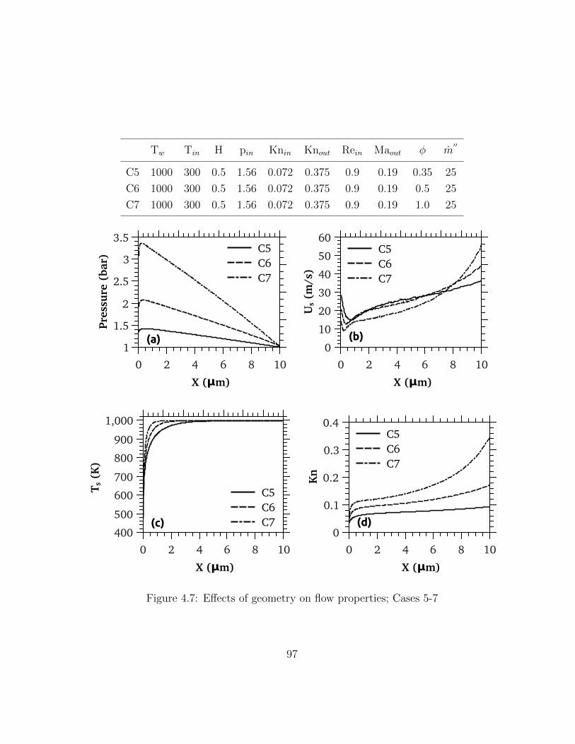
Tw Tin H pin Knin Knout Rein Maout φ m′′

C5 1000 300 0.5 1.56 0.072 0.375 0.9 0.19 0.35 25

C6 1000 300 0.5 1.56 0.072 0.375 0.9 0.19 0.5 25

C7 1000 300 0.5 1.56 0.072 0.375 0.9 0.19 1.0 25

Pres

sure

(ba

r)

1

1.5

2

2.5

3

3.5

X (μm)

0 2 4 6 8 10

C5C6C7

(a)

Us (

m/s

)

0

10

20

30

40

50

60

X (μm)

0 2 4 6 8 10

C5C6C7

(b)

Ts (

K)

400

500

600

700

800

900

1,000

X (μm)

0 2 4 6 8 10

C5C6C7(c)

Kn

0

0.1

0.2

0.3

0.4

X (μm)

0 2 4 6 8 10

C5C6C7

(d)

Figure 4.7: Effects of geometry on flow properties; Cases 5-7

97

Figures 4.8-4.13 show effects of various geometries on surface coverage of the species

participating in heterogeneous reactions. Due to the close relation, surface coverage graphs

of each species are followed by molar concentration graphs of the corresponding component

in the gas. As it was mentioned earlier, catalytic reactions start at 1µm and therefore, the

surface coverage of hydrogen θH∗ steps up at this point, seen in Figure 4.8. The starting

value of θH∗ is not affected by the geometry and is a function of flow and surface properties.

Generally, θH∗ decreases from this constant value for all channel heights and gets close to

zero at some distance. Due to the fact that all cases studied in this part are fuel lean

(φ = 0.28), the point at which θH∗ approaches zero falls within the channel. At this point,

the hydrogen concentration in the gas XH2 is low enough so that the hydrogen adsorption

rate is almost equal to the rate of hydrogen consumption on the surface. Thus, from this

point on, small amount of adsorbed hydrogen molecules will be left on the surface at steady

state conditions. This also reduces reaction rates for the rest of the channel and lack of

θH∗ becomes the limiting factor of surface reactions. Distributions of XH2 in Figure 4.8

also turn into a constant value from where θH∗ attains zero. Another notable point in this

figure is that XH2 has different values at the inlet for different channel heights despite the

fact that equivalence ratio is constant. The reason is that molar density of water is also

considered in evaluation of XH2 where as equivalence ratio is calculated just from molar

densities of reactants species.

While θH∗ is diminishing along the channel, adsorbed oxygen molecules are consumed

less and hence, θO∗ sharply increases as shown in Figure 4.9. Both θH∗ and XO2 become

constant from this point on, as expected. θH2O∗ increases up to this point due to high

reaction rates and decreases afterwards, and XH2O becomes constant. The noticeable point

here is that θH2O∗ for smaller channels is higher or almost equal to that of larger channels

for the entire length of the channel. This guarantees higher XH2O throughout the channel

due to higher desorption rate, confirmed by Figure 4.10. This can be explained by noting

that higher pressure values at lower channel sizes cause higher MCR (mass diffusion to the

surface). This leads to a higher adsorption rate for H2 and O2 and therefore, the conversion

rate will be higher. For example, the conversion rate of H2 is shown in Figure 4.11.

It is observed that H2 conversion rate is higher for smaller channels as expected; thus,

higher production rate of H2O results in greater values for θH2O∗ , and XH2O. However, the

98

conversion rate dramatically diminishes at the point where θH∗ goes to zero. This point

occurs earlier for smaller channels as the higher conversion rate of these cases quickly

consumes available H2 molecules adsorbed on the surface (see Figure 4.8). Moreover, gas

flow entering small channel sizes carries less amount of reactant molecules due to constant

mass flux and equivalence ratio. This together with the fact that available surface sites is

constant for all cases, result in even more reduction of the effective conversion length and

lowers concentrations of the reactants as observed in Figures 4.8 and 4.9. As an additional

result, greater portion of air/H2 molecules will be converted to water and therefore, the

water concentration for smaller channels is higher (see Figure 4.10). This directly points

out that the efficiency of the reactor arrangement of Figure 1.1 with smaller perforations

will be higher. Molar flow rate of H2 shown in Figure 4.12 clearly reveals that as the

channel height decreases the portion of H2 consumed in the reactions is higher. If the

efficiency for the reactor is defined as the ratio of H2 moles participating in the reactions

to the total amount of H2 entering the channel, this value varies from 82% for Case 1 to

99% for Case 4.

Figure 4.13 shows distributions of θOH∗ for different geometries. Due to the low coverage

of OH∗, desorption of OH ions to the gas flow is negligibly small. Moreover, gas reactions

are not simulated here as mentioned before and therefore, modelling OH desorption seems

pointless.

4.4.2 Effect of equivalence ratio

So far all Cases studied above were fuel lean (φ < 1). In this section effect of the higher

equivalence ratio, stoichiometric, and fuel rich conditions are investigated. By increasing

φ, a higher amount of H2 molecules is carried into the channel with the flow; therefore, the

effective reaction length (along which θH∗ is greater than zero) is extended. As shown in

Figure 4.14, for φ around 0.5 and higher, θH∗ has non zero values throughout the channel.

It is also observed that XH2 is higher than zero at φ ≥ 0.5 for the entire channel length.

The effect of higher values of φ on θO∗ is shown in Figure 4.15. As expected, θO∗ for Cases

4 and 5 rises rapidly right after θH∗ diminishes on the surface. However, for the rest of

the Cases, θO∗ is less than 10−5. This reveals that the limiting factor for the reactions

99

Tw Tin H pin Knin Knout Rein Maout φ m′′

[K] [K] [µm] [bar] [kg/m2·s]

C1 1000 300 2.0 1.12 0.025 0.095 3.6 0.19 0.28 25

C2 1000 300 1.0 1.29 0.044 0.19 1.8 0.19 0.28 25

C3 1000 300 0.75 1.4 0.054 0.25 1.3 0.19 0.28 25

C4 1000 300 0.5 1.56 0.072 0.375 0.9 0.19 0.28 25

θH

*

0

0.005

0.01

0.015

0.02

0 2 4 6 8 10

C1C2C3C4

XH

2

0

0.02

0.04

0.06

0.08

0.1

X (μm)0 2 4 6 8 10

Figure 4.8: Effects of geometry on θH∗ and XH2 ; Cases 1-4

100

Tw Tin H pin Knin Knout Rein Maout φ m′′

[K] [K] [µm] [bar] [kg/m2·s]

C1 1000 300 2.0 1.12 0.025 0.095 3.6 0.19 0.28 25

C2 1000 300 1.0 1.29 0.044 0.19 1.8 0.19 0.28 25

C3 1000 300 0.75 1.4 0.054 0.25 1.3 0.19 0.28 25

C4 1000 300 0.5 1.56 0.072 0.375 0.9 0.19 0.28 25

XO

2

0.060.08

0.10.120.140.160.18

0.2

X (μm)0 2 4 6 8 10

θO

*

0

0.2

0.4

0.6

0.8

0 2 4 6 8 10

C1C2C3C4

Figure 4.9: Effects of geometry on θO∗ and XO2 ; Cases 1-4

101

Tw Tin H pin Knin Knout Rein Maout φ m′′

[K] [K] [µm] [bar] [kg/m2·s]

C1 1000 300 2.0 1.12 0.025 0.095 3.6 0.19 0.28 25

C2 1000 300 1.0 1.29 0.044 0.19 1.8 0.19 0.28 25

C3 1000 300 0.75 1.4 0.054 0.25 1.3 0.19 0.28 25

C4 1000 300 0.5 1.56 0.072 0.375 0.9 0.19 0.28 25

θH

2O* (

×10

4 )

0

2

4

6

8

0 2 4 6 8 10

C1C2C3C4

XH

2O

00.05

0.10.150.2

0.250.3

X (μm)0 2 4 6 8 10

Figure 4.10: Effects of geometry on θH2O∗ and XH2O; Cases 1-4

102

H2

Cov

ersi

on R

ate

(mol

/m2 ·

s)

0

10

20

30

40

50

X (μm)

0 2 4 6 8 10

C1C2C3C4

Figure 4.11: Effect of geometry on conversion rate of H2; Cases 1-4

H2

Mol

ar f

low

×10

4 (m

ol/s

)

0

0.5

1

1.5

2

X (μm)0 2 4 6 8 10

C1C2C3C4

Figure 4.12: Effect of geometry on molar flow rate of H2 through the channel; Cases 1-4

103

Tw Tin H pin Knin Knout Rein Maout φ m′′

[K] [K] [µm] [bar] [kg/m2·s]

C1 1000 300 2.0 1.12 0.025 0.095 3.6 0.19 0.28 25

C2 1000 300 1.0 1.29 0.044 0.19 1.8 0.19 0.28 25

C3 1000 300 0.75 1.4 0.054 0.25 1.3 0.19 0.28 25

C4 1000 300 0.5 1.56 0.072 0.375 0.9 0.19 0.28 25

θO

H* (

×10

4 )

0

2

4

6

8

10

X (μm)

0 2 4 6 8 10

C1C2C3C4

Figure 4.13: Effects of geometry on θOH∗ ; Cases 1-4

104

here is θO∗ which itself is controlled by MCR of O2 and θPt∗ . For fuel lean Cases, both of

these controlling factors (MCR of O2 and θPt∗) are higher due to higher O2 content of the

gas flow and lower θH∗ . Therefore, increasing fuel (H2) content of the gas flow does not

expectedly enhance reaction rates considerably. This is confirmed in Figure 4.14 as XH2 is

elevated by almost a constant amount with increasing φ. This shows that the conversion

rate of H2 has almost the same distribution for stoichiometric and fuel rich Cases.

Figure 4.16 shows that θH2O∗ is higher for Cases 4 and 5 (very fuel lean Cases) before

they drop passing their effective reaction length. This proves the importance of the higher

θO∗ role for theses Cases. Another noticeable observation is that as φ increases from 0.5 for

Case 6 to 1.0 and 1.5 for Cases 7 and 8 respectively, θH2O∗ decreases for the entire channel.

This is also the result of the lower θO∗ at higher values of φ. This behaviour causes XH2O at

the channel outlet to have the greatest value for Case 6, an equal value for Cases 5 and 7,

and almost an equal value for Cases 4 and 8. Efficiencies of these Cases are directly related

to XH2O at the outlet and therefore, have the same distribution. As seen in Figure 4.16,

XH2O for fuel lean Cases has higher initial values due to higher θH2O∗ and becomes constant

after θH∗ drops. On the other hand, XH2O for fuel rich Cases continuously increases along

the channel but from a lower initial value. Overall, it can be concluded that there is a

trade off between the amount of H2 molecules available and the MCR of O2, making an

optimum value for φ which is about 0.5 for the current arrangement.

The cases studied so far had the same channel height of 500nm and as well all cases

studied in Section 4.4.1 were on the fuel lean side (φ <1). To study mutual effects of

geometry and φ, some cases with channel heights of 500nm, 1µm and 2µm at stoichiometric

and fuel rich (φ=1.5) conditions are studied. As shown in Figure 4.18, decreasing the

channel height amplifies the gradient of the θH∗ distribution whereas increasing φ mostly

elevates the θH∗ distribution than changing its gradient. This pattern is also seen for θO∗

in Figure 4.19. As discussed before, a steeper gradient of surface coverages means a higher

surface reaction rate which itself augments the amount of products. Therefore, as clearly

seen in Figure 4.20 decreasing the channel height has higher contribution on enhancing

the product concentration and the conversion efficiency. Another observation is that the

improvement made by increasing φ is higher for smaller channels due to higher surface to

volume ratio.

105

Tw Tin H pin Knin Knout Rein Maout φ m′′

[K] [K] [µm] [bar] [kg/m2·s]

C4 1000 300 0.5 1.56 0.072 0.375 0.9 0.19 0.28 25

C5 1000 300 0.5 1.56 0.072 0.375 0.9 0.19 0.35 25

C6 1000 300 0.5 1.56 0.072 0.375 0.9 0.19 0.5 25

C7 1000 300 0.5 1.56 0.072 0.375 0.9 0.19 1.0 25

C8 1000 300 0.5 1.56 0.072 0.375 0.9 0.19 1.5 25

XH

2

0

0.1

0.2

0.3

0.4

X (μm)0 2 4 6 8 10

θH

*

0

0.02

0.04

0.06

0.08

0 2 4 6 8 10

C4 C6C5 C7

C8

Figure 4.14: Effects of equivalence ratio on θH∗ and XH2 ; Cases 4–8

106

Tw Tin H pin Knin Knout Rein Maout φ m′′

[K] [K] [µm] [bar] [kg/m2·s]

C4 1000 300 0.5 1.56 0.072 0.375 0.9 0.19 0.28 25

C5 1000 300 0.5 1.56 0.072 0.375 0.9 0.19 0.35 25

C6 1000 300 0.5 1.56 0.072 0.375 0.9 0.19 0.5 25

C7 1000 300 0.5 1.56 0.072 0.375 0.9 0.19 1.0 25

C8 1000 300 0.5 1.56 0.072 0.375 0.9 0.19 1.5 25

θO

*

00.10.20.30.40.50.60.70.8

0 2 4 6 8 10

XO

2

0

0.05

0.1

0.15

0.2

X (μm)0 2 4 6 8 10

C6 C4C7 C5C8

Figure 4.15: Effects of equivalence ratio on θO∗ and XO2 ; Cases 4–8

107

Tw Tin H pin Knin Knout Rein Maout φ m′′

[K] [K] [µm] [bar] [kg/m2·s]

C4 1000 300 0.5 1.56 0.072 0.375 0.9 0.19 0.28 25

C5 1000 300 0.5 1.56 0.072 0.375 0.9 0.19 0.35 25

C6 1000 300 0.5 1.56 0.072 0.375 0.9 0.19 0.5 25

C7 1000 300 0.5 1.56 0.072 0.375 0.9 0.19 1.0 25

C8 1000 300 0.5 1.56 0.072 0.375 0.9 0.19 1.5 25

θH

2O* (

×10

4 )

0

2

4

6

8

10

0 2 4 6 8 10

XH

2O

0

0.1

0.2

0.3

0.4

X (μm)0 2 4 6 8 10

C4 C7C5 C8C6

Figure 4.16: Effects of equivalence ratio on θH2O∗ and XH2O; Cases 4–8

108

θO

H* (

×10

4 )

0

2

4

6

8

10

X (μm)

0 2 4 6 8 10

C4 C6C5 C7

C8

Figure 4.17: Effects of equivalence ratio on θOH∗ ; Cases 4–8

4.4.3 Effect of inlet temperature

Figure 4.21 demonstrates clearly that increasing inlet temperature from 300K (Case 4)

to 700K (Case 10) has almost no effect on wall reactions and gas concentrations. The

reason is that reactions on the surface is restrained by the molecular transfer from the

gas to the surface and vice versa. Adsorption and desorption processes which create this

molecular transfer are functions of the surface temperature and gas conditions adjacent

to the wall. The only variable property here is the inlet temperature of the gas; however,

as shown in Figure 4.7, the gas temperature next to the wall surface rises up to the wall

temperature very quickly due to conductive nature of micro/nano flows. Hence, reactions

on the surface has the same behaviour regardless of the inlet temperature. Practically, this

is a favourable result; because, the gas contained in the inlet plenum of the hypothetical

arrangement shown in Figure 1.1 will be affected by the high temperature of the perforated

disk through conduction. Therefore, controlling the inlet temperature of the gas flow

entering the channels is difficult if not impossible. The results of this section reveal that

maintaining the temperature of the gas entering the perforated disk will not affect the

performance of the reactions.

109

Tw Tin H pin Knin Knout Rein Maout φ m′′

C7 1000 300 0.5 1.56 0.072 0.375 0.9 0.19 1.0 25

C8 1000 300 0.5 1.56 0.072 0.375 0.9 0.19 1.5 25

C23 1000 300 1.0 1.29 0.04 0.187 1.8 0.19 1.0 25

C24 1000 300 2.0 1.12 0.025 0.095 3.6 0.19 1.0 25

C25 1000 300 1.0 1.29 0.04 0.187 1.8 0.19 1.5 25

C26 1000 300 2.0 1.12 0.025 0.095 3.6 0.19 1.5 25

XH

2

0.1

0.15

0.2

0.25

0.3

0.35

0.4

X (μm)0 2 4 6 8 10

θH

*

0

0.02

0.04

0.06

0.08

0 2 4 6 8 10

Case 23 Case 25Case 24 Case 26Case 7 Case 8

Figure 4.18: Effects of geometry on θH∗ at stoichiometric and fuel rich conditions

110

Tw Tin H pin Knin Knout Rein Maout φ m′′

C7 1000 300 0.5 1.56 0.072 0.375 0.9 0.19 1.0 25

C8 1000 300 0.5 1.56 0.072 0.375 0.9 0.19 1.5 25

C23 1000 300 1.0 1.29 0.04 0.187 1.8 0.19 1.0 25

C24 1000 300 2.0 1.12 0.025 0.095 3.6 0.19 1.0 25

C25 1000 300 1.0 1.29 0.04 0.187 1.8 0.19 1.5 25

C26 1000 300 2.0 1.12 0.025 0.095 3.6 0.19 1.5 25

XO

2

0

0.02

0.04

0.06

0.08

0.1

0.12

0.14

0.16

X (μm)0 2 4 6 8 10

Case 23Case 24

Case 7 Case 26Case 25 Case 8

θO

* (×

105 )

0

2

4

6

8

0 2 4 6 8 10

Figure 4.19: Effects of geometry on θO∗ at stoichiometric and fuel rich conditions

111

Tw Tin H pin Knin Knout Rein Maout φ m′′

C7 1000 300 0.5 1.56 0.072 0.375 0.9 0.19 1.0 25

C8 1000 300 0.5 1.56 0.072 0.375 0.9 0.19 1.5 25

C23 1000 300 1.0 1.29 0.04 0.187 1.8 0.19 1.0 25

C24 1000 300 2.0 1.12 0.025 0.095 3.6 0.19 1.0 25

C25 1000 300 1.0 1.29 0.04 0.187 1.8 0.19 1.5 25

C26 1000 300 2.0 1.12 0.025 0.095 3.6 0.19 1.5 25

XH

2O

0

0.05

0.1

0.15

0.2

0.25

0.3

0.35

X (μm)0 2 4 6 8 10

Case 23 Case 26Case 24 Case 8Case 7 Case 25

θH

2O* (

×10

3 )

0

0.1

0.2

0.3

0.4

0.5

0.6

0.7

0.8

0 2 4 6 8 10

Figure 4.20: Effects of geometry on θH2O∗ at stoichiometric and fuel rich conditions

112

Tw Tin H pin Knin Knout Rein Maout φ m′′

C4 1000 300 0.5 1.56 0.072 0.375 0.9 0.19 0.28 25

C9 1000 500 0.5 1.85 0.101 0.375 0.7 0.15 0.28 25

C10 1000 700 0.5 2.13 0.123 0.375 0.6 0.12 0.28 25

θH

*

0

0.005

0.01

0.015

0.02

0.025

XH

2

0

0.02

0.04

0.06

0.08

0.1

0 2 4 6 8 10

C4C9C10

θO

*

0

0.2

0.4

0.6

0.8

XO

2

0.060.080.10.120.140.160.18

0 2 4 6 8 10

C4C9C10

θH

2O* (

×10

4 )

0

2

4

6

8X

H2O

0.05

0.1

0.15

0.2

0.25

0.3

X (μm)

0 2 4 6 8 10

C4C9C10

Figure 4.21: Effects of inlet temperature on surface coverages; Cases 4, 9, and 10

113

4.4.4 Effects of wall temperature

Fuel lean Cases

Figure 4.22 shows effects of the wall temperature ranging from 600K to 1000K on θH∗ . As

seen, increasing surface temperature decreases initial θH∗ but lengthens effective reaction

length. To find the reason of higher θH∗ at lower wall temperatures, an isothermal flow

of Case 14 in which Tin=Tw=300K is studied. At this temperature no reactions will take

place on the surface and the results show that θH∗ is almost equal to unity and θO∗ is very

close to zero. It happens because of two reasons: first, H2 adsorption is of the first order in

terms of θPt∗ and second, MCR of H2 molecules at these conditions is more than twice as

that of O2. Consequently, H2 molecules occupy free Pt∗ sites on the catalytic surface faster

and hence, θPt∗ decreases. Lower θPt∗ reduces the chance of adsorption for O2 molecules

even more, since it is of second order with regards to θPt∗ . The above process takes place

when Tw <500K where surface reactions are inefficient. In such a case, surface reactions

are not triggered from the beginning of the catalytic section and start in the middle of

the channel. This leads to sudden changes in surface coverage values making the ODE

system unstable. In addition, the point at which reactions are triggered is close to the

outlet, leaving the reaction zone small and hence, inefficient. As Tw goes beyond 500K, H2

molecules adsorbed on the surface will be consumed by catalytic reactions limiting θH∗ to

a maximum value. It is clear that by further elevation of Tw, the rate of H2 conversion will

increase and therefore, maximum value of the θH∗ will be reduced. Another observation

from Figure 4.22 is shorter effective reaction length for lower Tw Cases. The reason is the

higher H2 conversion rate for these Cases due to higher θH∗ (see Figure 4.26). This reduces

XH2 next to the surface decreasing MCR of H2 molecules to a point where the O2 adsorption

exceeds H2 and as seen in Figure 4.23, θO∗ rises afterwards. It seems the opposite effects

of higher θH∗ and shorter effective reaction length lead to a noticeable result that the XH2

distribution is almost not affected by variations of θH∗ . The XO2 distribution also remains

the same despite obvious changes of reactant surface coverages. lower Tw also neutralizes

the acceleration caused by the upper bound of θH∗ .

Similar behaviour is observed for θH2O∗ and XH2O distributions shown in Figure 4.24.

As shown, increasing Tw from 600K to 1000K enhances XH2O at the outlet by about 8%.

114

In addition, θH2O∗ for lower Tw are significantly higher. This happens due to the lower

desorption of H2O at lower Tw. considering the fact that the conversion rate is almost

the same for all the cases explained above, θH2O∗ increases in order to compensate the

adverse effect of lower Tw. This is a noteworthy result suggesting that increasing Tw is not

critical due to its negligible contribution to the reactor performance for the H2 oxidation.

Practically, it is desirable to design the reactor to work with the minimum Tw at which

effective surface reactions is created saving energy and realizing the design. Figure 4.25

also shows higher θOH∗ for lower Tw. This behaviour results in higher θH2O∗ through

subreactions 6 and 8 listed in Table 4.1.

Stoichiometric and fuel rich Cases

To investigate effects of the wall temperature at higher values of φ, stoichiometric and

fuel rich (φ=1.5) conditions are considered. As shown in Figure 4.29, there is no water

production for Tw=400K since the H2 desorption rate is almost zero leaving no room for

O2 molecules to be adsorbed. By increasing Tw to 600K, there is a big jump in water

production as reactions start. Further elevation of Tw to 800K causes 18% more water

production in comparison to 4% for fuel lean Cases (φ=0.28); however, if Tw is increased

more to 1000K, there is almost no change in XH2O distribution for the catalytic length of

the channel. This behaviour is similar to that seen for fuel lean Cases and comes from the

same root. Figure 4.27 shows that θH∗ and XH2 dramatically decrease at high Tw. This

largely countervails the higher reaction rate caused by higher Tw and therefore, increasing

Tw does not considerably improve the conversion rate even at stoichiometric conditions.

Increasing the magnitude of φ to 1.5 also shows similar behaviour as represented in

Figure 4.32. As Tw goes up from 600K to 800K, the value of XH2O at the outlet rises by

25% and further elevation of Tw from 800K to 1000K increases XH2O by less than 4%.

In order to evaluate and compare the performance of the Cases studied in this section,

molar flow distributions of water produced in surface reactions are shown in Figure 4.33.

As observed, the water flow of Cases 7 and 19 have the same distributions. This again

confirms that increasing Tw beyond 800K has no effect on the conversion rate. Having a

fuel rich condition by increasing φ from 1 to 1.5 slightly decreases the water production

115

Tw Tin H pin Knin Knout Rein Maout φ m′′

C4 1000 300 0.5 1.56 0.072 0.375 0.9 0.19 0.28 25

C11 600 300 0.5 1.66 0.068 0.225 0.9 0.12 0.28 25

C12 700 300 0.5 1.64 0.069 0.262 0.9 0.14 0.28 25

C13 800 300 0.5 1.61 0.07 0.3 0.9 0.15 0.28 25

θH

*

0

0.05

0.1

0.15

0.2

0 2 4 6 8 10

C11C12C13C4

XH

2

0

0.02

0.04

0.06

0.08

0.1

X (μm)0 2 4 6 8 10

Figure 4.22: Effects of wall temperature on θH∗ and XH2

116

Tw Tin H pin Knin Knout Rein Maout φ m′′

C4 1000 300 0.5 1.56 0.072 0.375 0.9 0.19 0.28 25

C11 600 300 0.5 1.66 0.068 0.225 0.9 0.12 0.28 25

C12 700 300 0.5 1.64 0.069 0.262 0.9 0.14 0.28 25

C13 800 300 0.5 1.61 0.07 0.3 0.9 0.15 0.28 25

XO

2

0.060.08

0.10.120.140.160.18

X (μm)0 2 4 6 8 10

θO

*

0

0.2

0.4

0.6

0.8

1

0 2 4 6 8 10

C11C12C13C4

Figure 4.23: Effects of wall temperature on θO∗ and XO2

117

Tw Tin H pin Knin Knout Rein Maout φ m′′

C4 1000 300 0.5 1.56 0.072 0.375 0.9 0.19 0.28 25

C11 600 300 0.5 1.66 0.068 0.225 0.9 0.12 0.28 25

C12 700 300 0.5 1.64 0.069 0.262 0.9 0.14 0.28 25

C13 800 300 0.5 1.61 0.07 0.3 0.9 0.15 0.28 25

XH

2O

0.05

0.1

0.15

0.2

0.25

0.3

X (μm)0 2 4 6 8 10

θH

2O* (

×10

4 )

0

50

100

150

0 2 4 6 8 10

C11C12C13C4

Figure 4.24: Effects of wall temperature on θH2O∗ and XH2O

118

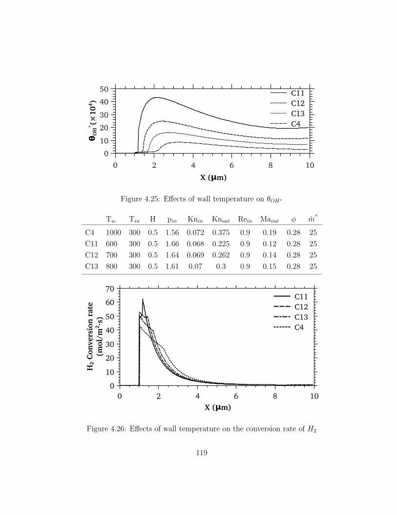
θO

H* (

×10

4 )

0

10

20

30

40

50

X (μm)

0 2 4 6 8 10

C11C12C13C4

Figure 4.25: Effects of wall temperature on θOH∗

Tw Tin H pin Knin Knout Rein Maout φ m′′

C4 1000 300 0.5 1.56 0.072 0.375 0.9 0.19 0.28 25

C11 600 300 0.5 1.66 0.068 0.225 0.9 0.12 0.28 25

C12 700 300 0.5 1.64 0.069 0.262 0.9 0.14 0.28 25

C13 800 300 0.5 1.61 0.07 0.3 0.9 0.15 0.28 25

H2

Con

vers

ion

rat

e(m

ol/m

2 ·s)

0

10

20

30

40

50

60

70

X (μm)0 2 4 6 8 10

C11C12C13C4

Figure 4.26: Effects of wall temperature on the conversion rate of H2

119

rate for Cases 8 and 22 as seen in Figure 4.33. In addition, the difference of Tw for these

two Cases makes very little change. Conversion efficiencies of Cases 7 and 19 are 65%

and 64.7%, Cases 8 and 22 are 50% and 47%, and Cases 18 and 21 are 60% and 42%,

respectively.

4.4.5 Effect of mass flux

Increasing the mass flux requires elevating inlet pressure as seen in Table 4.2 for Cases 4,

15, and 16. Higher inlet pressure results in higher MCR of gas molecules on the surface

leading to higher reactant surface coverages as shown in Figure 4.34. This augments the

surface reaction rate and therefore, H2 molecules adjacent to the surface are adsorbed and

converted more rapidly. This quickly lowers the MCR of H2 molecules and θH∗ along the

channel and hence, shortens the effective reaction length. Figure 4.36 also shows that high

reaction rate of Case 4 causes θH2O∗ to go initially higher than Case 15; however, θH2O∗

for Case 15 is higher for the rest of channel due to its longer effective reaction length. A

notable observation here is that although the mass flux is increased by a constant amount

from Case 16 to Case 4, results of Case 16 show larger differences from the other Cases.

Especially, both XH2O and θH2O∗ in Figure 4.36 are considerably higher for Case 16. It

seems that this behaviour is due to highly diffusive flow of this Case causing diffusion of

H2O molecules towards upstream. As shown in Figure 4.37, molar flow of H2 for all of the

cases drops to almost zero and it was found that efficiencies of them are all greater than

99%. This confirms that higher XH2O for Case 16 is not a result of a higher reaction rate

or a higher conversion efficiency. In fact, the amount of converted H2 molecules is higher

as the inlet mass flux increases due to the greater inlet molar flow.

120

Tw Tin H pin Knin Knout Rein Maout φ m′′

C7 1000 300 0.5 1.56 0.072 0.375 0.9 0.19 1.0 25

C17 400 300 0.5 1.7 0.066 0.15 0.9 0.08 1.0 25

C18 600 300 0.5 1.66 0.068 0.225 0.9 0.12 1.0 25

C19 800 300 0.5 1.61 0.07 0.3 0.9 0.15 1.0 25

XH

2

0.1

0.15

0.2

0.25

0.3

X (μm)0 2 4 6 8 10

θH

*

0

0.2

0.4

0.6

0.8

1

0 2 4 6 8 10

C17C18C19C7

Figure 4.27: Effects of the wall temperature on θH∗ at stoichiometric conditions.

121

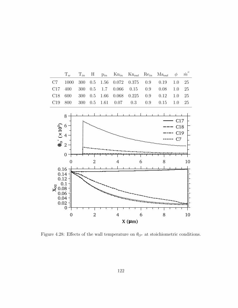
Tw Tin H pin Knin Knout Rein Maout φ m′′

C7 1000 300 0.5 1.56 0.072 0.375 0.9 0.19 1.0 25

C17 400 300 0.5 1.7 0.066 0.15 0.9 0.08 1.0 25

C18 600 300 0.5 1.66 0.068 0.225 0.9 0.12 1.0 25

C19 800 300 0.5 1.61 0.07 0.3 0.9 0.15 1.0 25

θO

* (×

105 )

0

2

4

6

8

0 2 4 6 8 10

C17C18C19C7

XO

2

00.020.040.060.08

0.10.120.140.16

X (μm)0 2 4 6 8 10

Figure 4.28: Effects of the wall temperature on θO∗ at stoichiometric conditions.

122

Tw Tin H pin Knin Knout Rein Maout φ m′′

C7 1000 300 0.5 1.56 0.072 0.375 0.9 0.19 1.0 25

C17 400 300 0.5 1.7 0.066 0.15 0.9 0.08 1.0 25

C18 600 300 0.5 1.66 0.068 0.225 0.9 0.12 1.0 25

C19 800 300 0.5 1.61 0.07 0.3 0.9 0.15 1.0 25

θH

2O* (

×10

3 )

0

2

4

6

8

10

0 2 4 6 8 10

XH

2O

0

0.1

0.2

0.3

0.4

X (μm)0 2 4 6 8 10

C17 C19C18 C7

Figure 4.29: Effects of the wall temperature on θH2O∗ at stoichiometric conditions.

123

Tw Tin H pin Knin Knout Rein Maout φ m′′

C8 1000 300 0.5 1.56 0.072 0.375 0.9 0.19 1.5 25

C20 400 300 0.5 1.7 0.07 0.15 0.9 0.08 1.5 25

C21 600 300 0.5 1.66 0.07 0.225 0.9 0.12 1.5 25

C22 800 300 0.5 1.61 0.07 0.3 0.9 0.15 1.5 25

θH

*

0

0.2

0.4

0.6

0.8

1

0 2 4 6 8 10

C20 C22C21 C8

XH

2

0.15

0.2

0.25

0.3

0.35

0.4

X (μm)0 2 4 6 8 10

Figure 4.30: Effects of the wall temperature on θH∗ at fuel rich conditions.

124

Tw Tin H pin Knin Knout Rein Maout φ m′′

C8 1000 300 0.5 1.56 0.072 0.375 0.9 0.19 1.5 25

C20 400 300 0.5 1.7 0.07 0.15 0.9 0.08 1.5 25

C21 600 300 0.5 1.66 0.07 0.225 0.9 0.12 1.5 25

C22 800 300 0.5 1.61 0.07 0.3 0.9 0.15 1.5 25

θO

* (×

105 )

0

1

2

3

4

5

0 2 4 6 8 10

C20C21C22C8

XO

2

00.020.040.060.08

0.10.120.140.16

X (μm)0 2 4 6 8 10

Figure 4.31: Effects of the wall temperature on θO∗ at fuel rich conditions.

125

Tw Tin H pin Knin Knout Rein Maout φ m′′

C8 1000 300 0.5 1.56 0.072 0.375 0.9 0.19 1.5 25

C20 400 300 0.5 1.7 0.07 0.15 0.9 0.08 1.5 25

C21 600 300 0.5 1.66 0.07 0.225 0.9 0.12 1.5 25

C22 800 300 0.5 1.61 0.07 0.3 0.9 0.15 1.5 25

θH

2O* (

×10

3 )

01234567

0 2 4 6 8 10

XH

2O

00.05

0.10.150.2

0.250.3

X (μm)0 2 4 6 8 10

C20 C22C21 C8

Figure 4.32: Effects of the wall temperature on θH2O∗ at fuel rich conditions.

126

Tw Tin H pin Knin Knout Rein Maout φ m′′

C7 1000 300 0.5 1.56 0.072 0.375 0.9 0.19 1.0 25

C8 1000 300 0.5 1.56 0.072 0.375 0.9 0.19 1.5 25

C18 600 300 0.5 1.66 0.068 0.225 0.9 0.12 1.0 25

C19 800 300 0.5 1.61 0.07 0.3 0.9 0.15 1.0 25

C21 600 300 0.5 1.66 0.07 0.225 0.9 0.12 1.5 25

C22 800 300 0.5 1.61 0.07 0.3 0.9 0.15 1.5 25

H2O

Mol

ar f

low

(m

ol/s

)×

104

0

0.2

0.4

0.6

0.8

1

X (μm)0 2 4 6 8 10

C7C8C18

C19C21C22

Figure 4.33: Molar flow of H2O at different Tw under stoichiometric and fuel rich conditions.

127

Tw Tin H pin Knin Knout Rein Maout φ m′′

C4 1000 300 0.5 1.56 0.072 0.375 0.9 0.19 0.28 25

C15 1000 300 0.5 1.33 0.072 0.375 0.5 0.12 0.28 15

C16 1000 300 0.5 1.11 0.072 0.375 0.2 0.04 0.28 5

XH

2

0

0.02

0.04

0.06

0.08

0.1

X (μm)0 2 4 6 8 10

θH

*

0

0.005

0.01

0.015

0.02

0 2 4 6 8 10

C16C15C4

Figure 4.34: Effects of mass flux on θH∗ and XH2 .

128

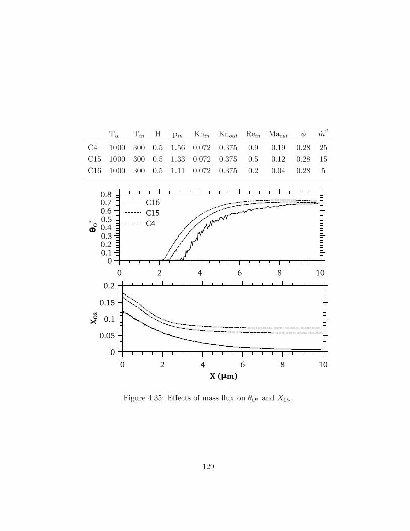
Tw Tin H pin Knin Knout Rein Maout φ m′′

C4 1000 300 0.5 1.56 0.072 0.375 0.9 0.19 0.28 25

C15 1000 300 0.5 1.33 0.072 0.375 0.5 0.12 0.28 15

C16 1000 300 0.5 1.11 0.072 0.375 0.2 0.04 0.28 5

θO

*

00.10.20.30.40.50.60.70.8

0 2 4 6 8 10

C16C15C4

XO

2

0

0.05

0.1

0.15

0.2

X (μm)0 2 4 6 8 10

Figure 4.35: Effects of mass flux on θO∗ and XO2 .

129

Tw Tin H pin Knin Knout Rein Maout φ m′′

C4 1000 300 0.5 1.56 0.072 0.375 0.9 0.19 0.28 25

C15 1000 300 0.5 1.33 0.072 0.375 0.5 0.12 0.28 15

C16 1000 300 0.5 1.11 0.072 0.375 0.2 0.04 0.28 5

XH

2O

00.10.20.30.40.50.6

X (μm)0 2 4 6 8 10

θH

2O* (

×10

4 )

0

2

4

6

8

10

0 2 4 6 8 10

C16C15C4

Figure 4.36: Effects of mass flux on θH2O∗ and XH2O.

130

Tw Tin H pin Knin Knout Rein Maout φ m′′

C4 1000 300 0.5 1.56 0.072 0.375 0.9 0.19 0.28 25

C15 1000 300 0.5 1.33 0.072 0.375 0.5 0.12 0.28 15

C16 1000 300 0.5 1.11 0.072 0.375 0.2 0.04 0.28 5

H2

Mol

ar f

low

×10

4 (m

ol/s

)

0

0.1

0.2

0.3

0.4

0.5

0.6

0.7

X (μm)0 2 4 6 8 10

Case 1Case 2Case 3

C16C15C4

Figure 4.37: Effects of mass flux on molar flow of H2

131

4.5 Summary

A method has been developed for coupling DSMC simulations with conventional modelling

of heterogeneous chemical reactions on catalytic surfaces. The proposed method can be

used in the transition regime (0.1<Kn<10) where Navier–Stokes equations break down.

This method has been applied to several lean Hydrogen/Air mixture flows in flat channels

with platinum coated walls. The results of a case in the slip regime have been compared

to conventional Navier–Stokes simulations employing slip/jump boundary conditions and

generally very good agreements were observed.

The accuracy of inlet and outlet boundary conditions have also been verified for some

sample cases. It has been shown that the mass flux and the equivalence ratio are effectively

kept constant at the inlet as well as atmospheric pressure at the outlet. Using the verified

code, effects of geometry, equivalence ratio, inlet and wall temperatures, and inlet mass

flux on the surface chemical reactions have been examined.

132

Chapter 5

Conclusions and future works

In this thesis, the fundamental behaviour of multi–component gas flows in micro/nano–

channels undergoing heterogeneous catalytic chemical reactions has been studied numeri-

cally. This work is primarily focused on nano–scale flows with recent and future applica-

tions in mind; especially, miniaturized energy sources such as micro–fuel cells and batteries.

Due to prevailing non–equilibrium conditions at these geometries, the DSMC method was

employed for its intrinsic ability in modelling rarefied gas flows and its flexibility to in-

corporate chemical reactions. The objective was achieved in three main steps which are

explained below followed by the observations:

1. Fluid dynamics and heat transfer of multi–component gas micro/nano–flows were inves-

tigated and the results were compared with corresponding data from the solution of the

Navier-Stokes equations with slip/jump boundary conditions:

Generally, very good agreements were observed for all the studied variables. For the

slip velocity, the maximum deviation was seen for higher inlet mass flux at the inlet of

the channel. The reason is the intense non–equilibrium conditions due to steep velocity

gradients at the entrance. The two methods also slightly digress from each other close to

the outlet boundary due to the rarefaction effects associated with the sudden pressure

drop. It was also seen that the difference between the results becomes higher as the

133

Knudsen number Kn increases (e.g. reducing the channel height) and/or as the velocity

and/or temperature gradients escalate.

Mass concentrations of the species showed very good agreement between the two meth-

ods. The maximum deviation was found to be about 8% for H2. Two reasons contribute

in building up this difference: first, the iterative nature of imposing constant mass flux

at the inlet causes a little less amount of molecules entering at the boundary than the

specified value. Second, the thermal velocity of H2 is very high due to its very light

molecules. This leads to high diffusion rates especially close to the walls where the gas

temperature is higher. The resulting upstream diffusion of H2 creates problems for the

Navier–Stokes method in maintaining a constant mass flux, since exclusive data is not

accessible in this method for each species.

Thermal results showed better agreement between the methods than fluid dynamics

data. The maximum temperature jump was captured at the inlet due to high temper-

ature and velocity gradients at that location. This quantity vanishes by approaching

the outlet and it was found that zero temperature gradient at the outlet leads to zero

temperature jump and as well, very good compliance of the methods. In addition, out-

let conditions such as the pseudo–reservoir length do not affect the thermal variable

distributions.

2. A new pressure boundary condition was introduced for multi–component gas flows, and

further improved using the Chapman–Enskog velocity distribution:

It is shown that velocity distribution plays an important role in calculating the number

flux across a surface; the key part of controlling a boundary pressure. The Maxwell

distribution is commonly used for this purpose, however, these values departed increas-

ingly along the channel from the number flux values sampled directly from DSMC. The

Chapman-Enskog distribution is employed as a remedy and the results are compared

to the first equivalent part of an extended channel, chosen as the reference solution. It

is found that this distribution has higher accuracy for simulating species compositions

at high Kn and low Peclet number Pe flows compared to the Maxwell distribution. A

distribution with higher order of accuracy, however, is required for heavier molecules in

cases of lower Kn or higher stream velocity.

134

3. A new method of coupling the flow field simulated by DSMC and surface chemical re-

actions simulated by conventional conservation ODE system was introduced, and the

effects of geometrical and boundary specifications on surface reactions were investigated:

The conversion rate of the reactor is higher for smaller channels due to the higher

inlet pressure caused by the constant mass flux, and the larger surface to volume ratio

at nano scales. This reduces the Mean Collision Rate (MCR) of H2 molecules on the

surface more rapidly for smaller channels and therefore, for fuel lean cases, the hydrogen

coverage θH∗ reaches zero at a shorter distance from the entrance within the channel.

Despite this, the water coverage θH2O∗ and the water molar concentration XH2O have

higher values throughout the channel. The comparison of the molar flow of H2 shows

that greater portion of H2 molecules entering the channel are converted inside smaller

channels and hence their performance is higher. However, for the smallest channel Case

4, about 95% of H2 is converted in the first half of the channel. This suggests that

adjusting the equivalence ratio proportional to the channel height can result in more

effective use of the channel length.

The optimum value of the equivalence ratio φ leading to the maximum efficiency is on

the fuel lean side with a value about 0.5. The reason is that a higher H2 content will

result in a lower θO∗ which is the limiting factor of the reactions.

Inlet temperature of the gas flow has almost no effect on the surface reactions. It was

found that the important temperature influencing the surface reactions (apart from the

wall temperature) is the gas temperature at the vicinity of the surface. This tempera-

ture rapidly rises to surface temperature minimizing the effect of its initial value. This

is a favourable result for using micro-reactors in applications since, high surface tem-

peratures of the channels will affect the upstream making it difficult to keep the inlet

temperature at an arbitrary low value.

It was observed that increasing the wall temperature Tw from 600K to 1000K makes

a small improvement (about 8%) on the efficiency. Three factors contribute to this

behaviour: higher θH∗ at lower Tw, higher surface reaction rates at higher Tw, and

shorter effective reaction length at lower Tw. These factors make complex distribu-

tions for surface coverages resulting in higher reaction rates at lower Tw; however, this

135

condition lasts for a shorter distance and therefore, overall amount of water produced

remains almost the same. The results for cases at stoichiometric and fuel rich (φ=1.5)

conditions showed about 20% rise in performance as Tw increases from 600K to 800K

but almost no change from 800K to 1000K. This is also a favourable result since lower

surface temperature will facilitate putting such reactors into application.

Increasing inlet mass flux increases surface coverages and therefore elevates reaction

rates. It was found that this enhancement does not change linearly with the inlet mass

flux and is higher for lower mass fluxes. The efficiency of the reactions however does not

change with increasing the inlet mass flux from 5kg/m2.s to 25kg/m2.s inside a channel

with 500nm height and remains about 99%. This means that by increasing the inlet

mass flux, the flow rate of products will be augmented.

There is a potential for further research based on the work described in this thesis to

examine different aspects of chemically reacting nano–flows. Some of the possibilities are

listed as follows:

Although parallel channels studied in this thesis seem easier for manufacturing and

utilization in wafer–like structured micro/nano–reactors, different geometries such as

circular or rectangular channel reactors can also be considered. Circular channel can

still be modeled using a 2–dimensional geometry domain by making some modifications

to the Direct Simulation Monte Carlo (DSMC) algorithm as suggested by Bird [1]. The

same methodology of this thesis for modeling surface chemical reactions can be adopted

on the catalytic walls. Possible applications can be thought of as using perforated plates

or porous media with circular nano–passages for the reactor core. Rectangular channels

with different aspect ratios are also of interest in practice. A 3–dimensional approach

is required for modeling this type of channels and therefore, molecular movement and

sampling routines should be modified.

In this thesis, heterogeneous chemical reactions are modeled using species conservation

ODE systems derived from the reaction mechanism. This gives the flexibility of using

available mechanisms; however, it is also possible to simulate surface reactions using

the generalized Monte Carlo method, mostly used for discrimination and extraction of

136

the reaction kinetics [62, 63]. There are two advantages associated with employing this

method: first, the nature of DSMC conforms well with such modeling schemes; therefore,

the implementation is easier and effective. Second, this will make the simulation capable

of handling special reactions that may happen in molecular scales and it is difficult to

distinct their mechanism with experiment. On the other hand, this kind of modeling

will add considerable computational cost to DSMC which itself is very demanding in

this regard.

In this thesis only catalytic oxidation of hydrogen was simulated. It is possible to incor-

porate different kinds of reactions as long as their kinetics are known. The decomposition

of ammonia on ruthenium or electro–chemical reactions taking place in micro–porous

membranes of fuel–cells are useful examples which are beneficial for developing future

miniaturized energy sources.

Effects of using different catalytic surface configurations like porous surfaces and packed

bed catalysts can also be studied using this method. Also, effects of diffusion of surface

species on the distribution of surface coverages can be considered. Surface diffusions

take place on the catalytic walls and are driven by surface coverage gradients.

As shown in the reacting flow simulations, rapid consumption of hydrogen leads to lack

of hydrogen molecules in the middle of the channel due to rarefaction. This makes dis-

tributions of surface coverages, gas concentrations, and consumption/production com-

plicated. Based on our studies, as the rarefaction increases, these distributions become

even more complicated since other reactant species especially oxygen will be totally

consumed as well. Therefore, in the present study, Kn < 0.4 was considered to deal

with the rarefaction effects on hydrogen. As the next step, reacting flows with higher

values of Kn can also be modeled and the obtained results can be interpreted based on

the explanations of the current work.

137

Appendices

138

Appendix A

Evaluation of tensors A, B, and C of

the Chapman–Enskog expansion

In this section, the equations required to evaluate the components of the matrices B, A,

and D used in Section 3.3 are presented. The derivation of these equations is similar to

[49, 50]; however, they are organized for easier implementation and to be consistent with

the terminology of this thesis. In addition, in Section A.3, the results of the developed

code for predicting the parameters involved in the equations are demonstrated and verified

against [49, 50].

A.1 Evaluation of the tensor B

The tensors B1

and B2, associated to the components 1 and 2 can be expanded in terms

of the following series:

B1

=∞∑

p=−∞p6=0

bpb(p)

1, B

2=

∞∑p=−∞p6=0

bpb(p)

2,

b(p)

1≡ 0, b(−p)

2≡ 0, (p < 0)

b(p)

1≡ S

(p−1)5/2 (C 2

1 )C 1C 1, b(−p)2≡ S

(p−1)5/2 (C 2

2 )C 2C 2, (p > 0)

(A.1)

139

In which, C = c′/Vmp and S(n)m (x) is defined as [28]:

S(n)m (x) =

n∑p=0

(n+m)!

p! (n− p)! (m+ p)!(−x)p (A.2)

The magnitudes of Sonine polynomial terms rapidly drop to zero as their order increases

and therefore, we just consider the first order term S(0)m (x) following the Chapman-Enskog

methodology. This way, B1

and B2

are reduced to B1

= b1C 1C 1 and B2

= b−1C 2C 2 and

the values of b1 and b−1 are obtained using the following system of equations:[b−1−1 b−11

b1−1 b11

][b−1

b1

]=

[β−1

β1

](A.3)

where the values of β are:

β−1 = 52n2/n

20, β1 = 5

2n1/n

20, (A.4)

The values of bpq in Equation (A.3) are related to the molecular properties and the model

of molecular interaction and are expressed as [49]:

b−1−1 = x22[4Ω

(2)2 (2)] + x1x2

803

(M1M2)Ω(1)12 (1) + 8M2

1 Ω(2)12 (2)

b−11 = b1−1 = x1x2

−80

3(M1M2)Ω

(1)12 (1) + 8M1M2Ω

(2)12 (2)

b11 = x2

1[4Ω(2)1 (2)] + x1x2

803

(M1M2)Ω(1)12 (1) + 8M2

2 Ω(2)12 (2)

(A.5)

where Ω(`)p (r) are defined as [28]:

Ω(`)12 (r) =

1

2σ2

12

(2πkT

m0M1M2

)1/2

W(`)12 (r) (A.6)

Ω(`)1 (r) = σ2

1

(πkT

m1

)1/2

W(`)1 (r) (A.7)

Ω(`)2 (r) = σ2

2

(πkT

m2

)1/2

W(`)2 (r) (A.8)

where W integrals are:

W (`)q (r) = 2

∞∫0

exp(−g2)g2r+3

π∫0

(1− cos` χ

)( b

σq

)d

(b

σq

)dg (A.9)

140

in which, parameters b and χ are associated with the molecular collision model. The

Hard Sphere (HS) collision model is used in this study in which, b is related to χ as

b = −σ12cos(χ/2). Substituting this into Equation (A.9) gives:

W (`)q (r) =

1

4

[2− 1

1 + `

(1 + (−1)`

)](1 + r)! (A.10)

which is independent of q. Using the equations of this section, the procedure of determining

tensor B is to substitute values of bpq and β calculated from Equation (A.5) and Equa-

tion (A.4) into equation Equation (A.3), and solving the corresponding system of linear

equations. This gives the magnitudes of bp by which the components of B are calculated

from Equation (A.1).

A.2 Evaluation of vectors A and D

The Chapman–Enskog solution of vectors A and D, which are the remaining unknowns of

the perturbation function Φ1, starts with the definition of A, as follows [28]:

A = A− kTD (A.11)

where, kT is the thermal diffusion coefficient for the gas mixture and will be independently

evaluated from vector D components at the end of the solution. The vectors A and D are

then expressed in terms of the following series:

A1 =∞∑

p=−∞p 6=0

apa(p)1 , A2 =

∞∑p=−∞p 6=0

apa(p)2 , (A.12)

D1 =∞∑

p=−∞

dpa(p)1 , D2 =

∞∑p=−∞

dpa(p)2 , (A.13)

141

where the components of the vector a(p) are [28]:

a(p)1 = a

(0)1 = M

1/21 ρ2C 1/ρ0, (p = 0),

a(−p)2 = a

(0)2 = −M1/2

2 ρ1C 2/ρ0, (p = 0),

a(p)1 = S

(p)3/2(C 2

1 )C 1, (p > 0),

a(−p)2 = S

(p)3/2(C 2

2 )C 2, (p > 0),

a(p)1 = 0, (p < 0),

a(−p)2 = 0, (p < 0),

(A.14)

Using the same argument for evaluation of b1 and b−1, the first order terms of Sonine

polynomials are kept, S(0)m (x), and then the values of ap and dp shown in Equation (A.12)

and Equation (A.13) are obtained from:[a−1−1 a−11

a1−1 a11

][a−1

a1

]=

[α−1

α1

](A.15)

and: a−1−1 a−10 a−11

a0−1 a00 a01

a1−1 a10 a11

d−1

d0

d1

=

0

δ0

0

(A.16)

In the above equations, the values of α and σ for each species are calculated from:

α1 = −15

4

n1

n20

(2kT

m1

)1/2

, α−1 = −15

4

n2

n20

(2kT

m2

)1/2

(A.17)

and:

δ0 = − 3

2n0

(2kT

m0

)1/2

(A.18)

142

and the components of coefficient matrices are evaluated from [50]:

a−1−1 = x22

4Ω

(2)2 (2)

+ x1x2

10(5M3

1 + 6M1M22 )Ω

(1)12 (1)

−40M31 Ω

(1)12 (2) + 8M3

1 Ω(1)12 (3) + 16M2

1M2Ω(2)12 (2)

a−10 = x1x2

−20(M2

1M1/22 )Ω

(1)12 (1) + 8(M2

1M1/22 )Ω

(1)12 (2)

a−11 = x1x2

−110M

3/21 M

3/22 Ω

(1)12 (1) + 40M

3/21 M

3/22 Ω

(1)12 (2)

−8M3/21 M

3/22 Ω

(1)12 (3) + 16M

3/21 M

3/22 Ω

(2)12 (2))

a00 = x1x2

8M1M2Ω

(1)12 (1)

a10 = x1x2

20(M

1/21 M2

2 )Ω(1)12 (1)− 8(M

1/21 M2

2 )Ω(1)12 (2)

a11 = x2

1

4Ω

(2)1 (2)

+ x1x2

10(5M3

2 + 6M21M2)Ω

(1)12 (1)

−40M32 Ω

(1)12 (2) + 8M3

2 Ω(1)12 (3) + 16M2

2M1Ω(2)12 (2)

(A.19)

where the omega functions are the same as Equation (A.6-A.8). It should be noted that

the components of the coefficient matrix a presented above, are off-diagonally symmetric,

such that a01 = a10, a0−1 = a−10 and a1−1 = a−11. Now, we are in a position to evaluate

the vectors A and D. This is done by substituting Equation (A.18) and Equation (A.19)

into Equation (A.16), and also substituting Equation (A.17) and Equation (A.19) into

Equation (A.15) and solving the corresponding system of linear equations. This way, the

values of ap and dp are obtained, which are then used together with Equation (A.14) in

order to evaluate the vectors A and D for each component. The value of kT is required for

further progression, which is calculated from [28]:

kT = −5

2

(x1M

−1/21 d1 + x2M

−1/22 d−1

)/d0 (A.20)

Having the values of kT , A and D, it is then possible to evaluate vector A from Equa-

tion (A.11).

A.3 Chapman-Enskog parameters

The values of (b−1, b1) are compared with [49] and the values of (a−1, a1, d0) are compared

with [50] for two binary mixture of noble gases, He/Ne and Ar/Kr, as are shown in Ta-

143

Table A.1: The molecular mass and diameter data used in [49, 50]

Molecular massa Molecular diametera

(amu) ×10−10 (m)

He 4.002602 2.193

Ne 20.1797 2.602

Ar 39.948 3.659

Kr 83.897 4.199

a The data are at 0C and 1 atm.

ble A.2 and Table A.3 respectively. The agreement of the results implies that the procedure

of calculating these parameters is correctly implemented in the prepared code for the cur-

rent study. The first order values of (d−1, d1) are not listed in the mentioned references;

however, the verification of the values of transport coefficients, ensures the accurate calcu-

lation of parameters correctly. The molecular masses and diameters of He, Ne, Ar and Kr

used by Tipton et al. [49] are shown in Table A.1.

144

Table A.2: The comparison of (b−1, b1) calculated from Equation (A.3) with [49]

Current studya Tipton IIa

x1 b1 b−1 b1 b−1

He:Ne 0.1 2.997 1.382 2.998 1.382

0.5 3.521 1.556 3.523 1.556

0.9 4.230 1.758 4.232 1.758

Ar:Kr 0.1 2.309 1.694 2.310 1.694

0.5 2.526 1.840 2.526 1.840

0.9 2.781 2.009 2.782 2.009

a All values are scaled as 1× 1010 (secˆ-1)

Table A.3: The comparison of (a−1, a1, d0) calculated from Equation (A.15) and Equa-

tion (A.16) with [50]

Current studya Tipton IIIa

x1 a1 a−1 d0 a1 a−1 d0

He:Ne 0.1 -15.844 -20.474 4.331 -15.849 -20.485 4.334

0.5 -19.382 -20.971 1.535 -19.390 -20.983 1.536

0.9 -26.193 -23.471 4.144 -26.206 -23.484 4.147

Ar:Kr 0.1 -7.644 -7.959 1.255 -7.649 -7.963 1.256

0.5 -8.530 -8.418 4.474 -8.534 -8.422 4.477

0.9 -9.924 -9.286 1.224 -9.929 -9.290 1.225

a The values of a1 and a−1 are scaled as 1× 108 (m) and the values

of d0 are scaled as 1× 106 (m)

145

Appendix B

Statistical sampling procedure

During the DSMC solution, it is required to sample a random value from a probability

distribution function. The method employed by DSMC is the inverse cumulative method

in which, the cumulative distribution function of a variable like x is equated by a randomly

generated number in the range of zero to one, and accordingly, the value of x is obtained.

The distribution function is defined as the probability magnitude of the variable, x, between

x and x + dx which is fxdx. Referring to the definition of the distribution function, its

integration over the whole range of x is equal to one:

b∫a

fxdx = 1 (B.1)

Accordingly, the cumulative distribution function is defined as:

Fx =

x∫a

fxdx (B.2)

The value of the Fx is restricted between zero and one; therefore, cumulative distribution

can be considered as the probability of a property with the distribution of fx at point x.

To sample a random value from a distribution fx, a random value is generated between 0

and 1 and substituted for Fx. Then, the corresponding value of x can be calculated from

146

the inverse of the cumulative function Equation (B.2). Such a procedure is straightforward

whenever Fx has an explicit reversible form; otherwise, the acceptance–rejection method

has to be used. This method is more efficient in comparison to other alternatives like the

Newton iteration method [64]. As an example, the Maxwellian equilibrium distribution

function Equation (3.7) for each component of the thermal velocity is considered:

fv′x =(β/√π)

exp(−β2v′

2x

)(B.3)

Its corresponding cumulative distribution function is:

Fv′x = 12

(1 + erf (βv′x)) (B.4)

in which, erf represents the standard error function that is not invertible, and β = 1/Vmp

where Vmp is obtained from Equation (2.36). In the acceptance–rejection algorithm, the

distribution function is normalized by a general function ex, which must be larger than fx

for the entire x domain. A random x is chosen among its range. If fx/ex > Rf then the

chosen x is accepted; otherwise, it is rejected and the loop must be restarted by choosing

a new random x until an accepted value is attained. In order to obtain the optimum

algorithm, ex is normally chosen as fx)max, which can be predicted in the DSMC method

functions. Using this procedure, fv′x/fv′x)max for the Maxwellian velocity distribution is

evaluated from:

fv′x/fv′x)max = exp(−β2v′

2x

)(B.5)

Choosing v′x randomly from the f ′v′x distribution between −3Vmp to 3Vmp (this range is

the most effective restriction of -∞ to +∞ for the molecular velocity) is done by the direct

method as:

f ′v′x = 1/(3/β − (−3/β)) = β/6 (B.6)

The corresponding cumulative distribution function is:

F ′v′x =

x∫−3/β

f ′v′xdv′x = βv′x/6 + 1

2(B.7)

Equating F ′v′x to a random number, Rf1, gives the explicit expression for v′x as:

v′x = 3 (2Rf1 − 1) /β (B.8)

147

Substituting into Equation B.5 results in:

fv′x/fv′x)max = exp(−9 (2Rf1 − 1)2) (B.9)

After calculating fv′x/fv′x)max the second random number, Rf2, is generated, and the pro-

cess repeated from Equation B.8 until fv′x/fv′x)max < Rf2. The accepted v′x is a random

selection from the Maxwellian velocity distribution. A special case is available when select-

ing two or three components of molecular velocities from Maxwellian distribution in the

initialization process, where a direct method can be used to circumvent the time consum-

ing acceptance–rejection process. The probability of two values of components of thermal

velocity simultaneously in an element of the velocity space is the product of both single

probabilities:

fv′xdv′x · fv′ydv′y = (β2/π) exp

(−β2v′2x

)exp

(−β2v′2y

)dv′xdv

′y =

(β2/π) exp(−β2

(v′2x + v′2y

))dv′xdv

′y

(B.10)

Changing the variables as follows:

v′x = r · cos(θ)

v′y = r · sin(θ)(B.11)

and substituting to the previous equation, gives:

fv′xdv′x · fv′ydv′y = (β2/π) exp (−β2r2) rdrdθ =

exp (−β2r2) d (β2r2) dθ/(2π)(B.12)

therefore:

f−β2r2 = exp(−β2r2

)(B.13)

so that r and θ are sampled by:

θ = 2πRf

r =√−ln(Rf )/β

(B.14)

and then velocity components are obtained from Equation B.11 [1]. Another concern is

to sample the Larsen–Borgnakke distribution with regard to the internal energy redistri-

bution. Recently, a faster method has been developed by Sun et al. [64] to expedite the

148

process. They used a variable change as:

y =

(Ea

Ea + Eb

)1/8

g = log2

(ζa

ζa + ζb

) (B.15)

According to the definition of y, the Larsen–Borgnakke distribution [35] becomes:

fy =gΓ(ζa + ζb)

Γ(ζa)Γ(ζb)(yg)ζa−1/g (1− yg)ζb−1 (B.16)

And by integration and normalization, the probability ratio for a specific value of y is

obtained as:

P

Pmax=

(ζa + ζb − 1− 1/g

ζa − 1/gyg)ζa−1/g (

ζa + ζb − 1− 1/g

ζb − 1(1− yg)

)ζb−1

(B.17)

Although change of variables back and forth increases the computational demand, the

average number of iterations is reduced considerably; especially, for low energy fraction.

149

Appendix C

Navier–Stokes equations with

slip–jump boundary conditions

The equations of this sections are adopted from the author’s paper [21].

C.1 Navier-Stokes equations

The governing mass, momentum, energy, and species continuity equations for steady, lam-

inar, non–reacting multi–component gas flows are [65]:

∇ · (ρV) = 0 (C.1)

∇ · (ρVV) = −∇p+∇ ·[µ(∇V +∇VT

)− 2

3µ (∇ ·V) I

](C.2)

∇ · (ρVh) = −∇ ·

(−λ∇T +

Ng∑k=1

hkJk

)+ Φ (C.3)

∇ · (ρVYk) = −∇ · Jk (C.4)

Here, ρ is the mixture density, V is the mass–averaged velocity vector, p and µ are pressure

and viscosity, I is the identity tensor, λ is the mixture conductivity, h is the mixture

150

enthalpy, Φ is the viscous dissipation term, Ng is the total number of gas phase species, Jk

is the mass diffusion flux, Yk is the mass fraction, cp,k is the specific heat capacity, and hk

is the enthalpy of the kth species. The species diffusion mass flux Jk is determined using

the multi-component diffusion equation as [65]:

Jk =ρwkw2

Ng∑j=1

wjDkj∇Xj −DTk

1

T∇T (C.5)

In this equation, Xk is the mole fraction and wk is the molar mass of species ”k”, w is the

mixture molar mass, Dkj is the tensor of ordinary diffusion coefficients, and DTk are the

thermal diffusion coefficients [66].

Boundary Conditions

At the channel inlet, the mass flux of each species is constant. Since the mass flux of

each species is constant at the channel inlet, the overall inlet mass flux will also remain

constant. The inlet mass flux of each species consists of the diffusion mass flux and the

convective mass flux of that species. When there is a positive diffusive flux of one species

into the channel, in order to keep the mass flux constant, the inlet mass fraction of that

species should be adjusted (lowered) accordingly. This way, the total mass flux of that

species, ~m′′

k = ρYkV + Jk remains constant. This procedure eliminates the inaccuracy

in ignoring the incoming (or outgoing) inlet diffusive mass flux of species especially at

low Peclet number flows. At each iteration, the inlet mass fraction of all species Yk and

the mass-averaged inlet velocity V are calculated using ~m′′

k = ρYkV + Jk = const (Ng

constraints) along with∑Ng

k=1 Yk = 1. The diffusive fluxes of species Jk are calculated from

the previous iteration.

In the slip flow regime, the continuum equations for mass, momentum and energy

conservation, described earlier, can still be employed but proper slip/jump boundary con-

ditions should be specified to account for non–equilibrium effects in the Knudsen layer.

In the present work, the set of velocity slip and temperature jump boundary conditions,

proposed by Qazi Zade et al. [45] for multicomponent mixtures (including reacting mix-

tures [42]), are employed at the wall. These boundary conditions, developed based on the

kinetic theory of gases, can be summarized as:

151

us =

∑Ng

k=1ρk,s√wk

[θk

(λk

5ρR∂ lnT∂x− Jkx

ρk

)− (2− θk)

wτxyk

ρwk

√π

2RkT

]s∑Ng

k=1ρk,s√wk

[θk

(1 +

τyyk

2p

)+ (2− θk) Jky

ρk

√π

2RkT

]s

(C.6)

TsTw

=

∑Ng

k=1ρk

w3/2k

[γ+1

4(γ−1)+ U2

4RkTw

] [θk

(1 +

τyyk

2p

)+

Jky(2−θk)

ρk

√π

2RkT

]s∑Ng

k=1ρk

w3/2k

[5(2−θk)

4

√π

2RkT

(Jkyρk− 2λk

5ρR∂ lnT∂y

)+ θkJ1

]s

(C.7)

(ρYk)w(ρYk)s

(TwTs

)1/2

(θk − γk) = θk

(1 +

τ yyk2p

)+ (2− θk)

Jkyρk,s

√π

2RkTs(C.8)

where us and Ts are the velocity and temperature of the gas at the edge of the Knudsen

layer, γ is the specific heat ratio, Rk is the gas constant of the kth species and:

τxyk = −µk(∂Ux∂y

+∂Uy∂x

)(C.9a)

τ yyk =2µk3

(∂Ux∂x

+∂Uz∂z− 2

∂Uy∂y

)(C.9b)

J1 =γ + 1

4 (γ − 1)+τ yyk8p

(3γ − 1)

(γ − 1)+

5− 3γ

4 (γ − 1)

Jkyρk

√π

2RkT(C.9c)

The diffusion flux of species in these equation are only important in catalytic reacting

flows where some species are produced or consumed at the wall. These terms are only

retained for completeness and obviously are zero in the present work. The accommodation

coefficient θ is equal to zero for specular reflection at the wall and equal to 1 for diffuse

reflection [28]. For most engineering applications they are close to unity and for comparison

purposes they are assumed to be equal to 1 in the present work.

Numerical Implementation

The governing equations were discretized using the finite volume method. A non-staggered

(colocated) arrangement was employed for the solution of the flow field following the Rhie

and Chow [67] formulation. Implementing the Pressure Weighted Interpolation Method

152

(PWIM), the control volume face velocities are related to nodal pressure values. A linear

deferred correction scheme is also used to improve the upwind approximation in descretizing

the advection terms. The mixture transport properties as well as the pure species properties

are obtained using the CHEMKIN database [68].

The finite volume code has been validated in the no–slip regime by comparing the

simulation results with experimental and numerical data of Appel et al. [69]. The details

can be found in Qazi Zade et al. [60], and therefore, are not repeated here.

153

References

[1] G. Bird, Molecular Gas Dynamics and the Direct Simulation Monte Carlo, Oxford

Science Publication, 1994.

[2] G. Karniadakis, A. Beskok, N. Aluru, Microflows and Nanoflows; fundamentals and

simulation, Springer, 2005.

[3] T. Doi, Numerical analysis of oscillatory Couette flow of a rarefied gas on the basis

of the linearized Boltzmann equation, Vacuum 84 (2009) 734–737. doi:10.1016/j.

vacuum.2009.10.007.

[4] R. D. Garcia, C. E. Siewert, The linearized Boltzmann equation: Sound-wave prop-

agation in a rarefied gas, Zeitschrift Fur Angewandte Mathematik Und Physik 57

(2005) 94–122. doi:10.1007/s00033-005-0007-8.

[5] O. A. Sinkevich, A. M. Semenov, Solution of the Boltzmann equation by expanding

the distribution function with several time and coordinate scales in the enskog series in

knudsen parameter, Technical Physics 48 (2003) 1221–1225. doi:10.1134/1.1620111.

[6] D. Valougeorgis, S. Naris, Analytical Lattice Boltzmann Solutions for Thermal Flow

Problems, Transport Theory and Statistical Physics 32 (2003) 645–656. doi:10.1081/

TT-120025070.

[7] T. Abe, Takashi, Derivation of the Lattice Boltzmann Method by Means of the Dis-

crete Ordinate Method for the Boltzmann Equation, Journal of Computational Physics

131 (1997) 241–246. doi:10.1006/jcph.1996.5595.

154

[8] F. Sharipov, L. G. Cumin, D. Kalempa, Plane Couette flow of binary gaseous mixture

in the whole range of the Knudsen number, European Journal of Mechanics B-fluids

23 (2004) 899–906. doi:10.1016/j.euromechflu.2004.03.002.

[9] S. Ching, Y. Zhiqiang, Direct numerical test of the B-G-K model equation by the

DSMC method, Acta Mechanica Sinica 16 (2000) 133–140. doi:10.1007/BF02486705.

[10] G. A. Bird, Approach to Translational Equilibrium in a Rigid Sphere Gas, Physics of

Fluids 6 (1963) 1518–1519. doi:10.1063/1.1710976.

[11] M. Ikegawa, J. Kobayashi, Development of a rarefied gas flow simulation using the

direct simulation Monte Carlo method, series 2, JSME International Journal 33 (3)

(1990) 463–467.

[12] E. S. Piekos, K. S. Breuer, Numerical Modeling of Micromechanical Devices Using the

Direct Simulation Monte Carlo Method, Journal of Fluids Engineering-transactions

of The Asme 118. doi:10.1115/1.2817781.

[13] Y. Fang, W. Liou, Computations of the flow and heat transfer in mirodevices using

DSMC with implicit boundary conditions, Journal of Heat Transfer 124 (2002) 338–

345.

[14] M. Wang, Z. Li, Simulations for gas flows in microgeometries using the direct simu-

lation Monte Carlo method, International Journal of Heat and Fluid Flow 25 (2004)

975–985.

[15] Q. Wang, X. Yan, Q. He, Heat-flux-specified boundary treatment for gas flow and heat

transfer in microchannel using direct simulation Monte Carlo method, Internatonal

Journal for Numerical Methods in Engineering 74 (2008) 1109–1127.

[16] M. Le, I. Hassan, DSMC simulation of gas mixing in T-shape micromixer, Applied

Thermal Engineering 27 (2007) 2370–2377. doi:10.1016/j.applthermaleng.2007.

03.012.

155

[17] F. Yan, B. . Farouk, Numerical simulation of gas flow and mixing in a microchannel

using the direct simulation Monte Carlo method, Microscale Thermophysical Engi-

neering 6 (2002) 235–251.

[18] G. Bird, Chemical reactions in dsmc, in: AIP Conference Proceedings, Vol. 1333,

2011, pp. 1195–1202.

[19] C. Lilley, M. Macrossan, A macroscopic chemistry method for the direct simulation

of gas flows, Physics of Fluids 16 (2004) 2054–2067.

[20] C. Cercignani, A. Frezzotti, S. Sibilla, Hypersonic rarefied flows DSMC analysis by a

simplified chemical model, Meccanica 30 (1995) 93–104.

[21] A. Qazi Zade, A. Ahmadzadegan, M. Renksizbulut, A detailed comparison between

navier–stokes and dsmc simulations of multicomponent gaseous flow in microchannels,

International Journal of Heat and Mass Transfer 55 (17) (2012) 4673–4681.

[22] A. Ahmadzadegan, J. Wen, M. Renksizbulut, The role of the velocity distribution

in the DSMC pressure boundary condition for gas mixtures, International Journal of

Modern Physics C 23 (2012) 1250087.

[23] W. Wagner, A convergence proof for Bird’s direct simulation Monte Carlo method for

the Boltzmann equation, Journal of Statistical Physics 66 (1992) 1011–1044.

[24] H. Struchtrup, Macroscopic Transport Equations for Rarefied Gas Flows: Approxima-

tion Methods in Kinetic Theory, Interaction of Mechanics and Mathematics, Springer,

2005.

[25] K. Koura, H. Matsumoto, Variable soft sphere molecular model for inverse-power-law

or lennard-jones potential, Physics of Fluids A 3 (1991) 2459–2465.

[26] K. Koura, H. Matsumoto, Variable soft sphere molecular model for air species, Physics

of Fluids A 4 (1992) 1083.

[27] H. A. Hassan, D. B. Hash, A generalized hard-sphere model for Monte Carlo simula-

tion, Physics of Fluids 5 (1993) 738–744. doi:10.1063/1.858656.

156

[28] S. Chapman, T. Cowling, The Mathematical Theory of Non-uniform Gases, 3rd Edi-

tion, Cambridge University Press, 2003.

[29] C. Borgnakke, P. Larsen, Statistical collision model for monte carlo simulation of

polyatomic gas mixture, Journal of Computational Physics 18 (1975) 405–420.

[30] R. Barber, D. Emerson, Challenges in modeling gas-phase flow in microchannels: From

slip to transition, Heat Transfer Engineering 27 (2006) 3–12.

[31] C. Shen, Rarefied Gas Dynamics, Fundamentals, Simulations and Micro Flows,

Springer, 2005.

[32] C. Cai, I. Boyd, J. Fan, Direct simulation method for low-speed microchannel flows,

Journal of Thermophysics and Heat Transfer 14 (3) (2000) 368–378.

[33] P. S. Prasanth, J. K. Kakkassery, Direct simulation Monte Carlo (DSMC): A numerical

method for transition-regime flows-A review, Journal of the Indian Institute of Science

86 (2006) 169–192.

[34] G. A. Bird, M. A. Gallis, J. R. Torczynski, D. J. Rader, Accuracy and efficiency of the

sophisticated direct simulation Monte Carlo algorithm for simulating noncontinuum

gas flows, Physics of Fluids 21. doi:10.1063/1.3067865.

[35] D. I. Pullin, Kinetic models for polyatomic molecules with phenomenological energy

exchange, Physics of Fluids 21 (1978) 209–216. doi:10.1063/1.862215.

[36] S. Varoutis, C. Day, F. Sharipov, Rarefied gas flow through channels of finite length

at various pressure ratios, Vacuum 86 (12) (2012) 1952 – 1959.

[37] S. Pantazis, D. Valougeorgis, F. Sharipov, End corrections for rarefied gas flows

through capillaries of finite length, Vacuum 97 (2013) 26 – 29.

[38] E. Roohi, M. Darbandi, V. Mirjalili, Direct Simulation Monte Carlo Solution of Sub-

sonic Flow Through Micro/Nanoscale Channels, Journal of Heat Transfer-transactions

of The Asme 131. doi:10.1115/1.3139105.

157

[39] R. Fernandez-Feria, On the Gas Dynamics of Binary Gas Mixtures with Large Mass

Disparity, Yale University, 1987.

[40] A. Q. Zade, M. Renksizbulut, J. Friedman, Homogeneous oxidation of hydrogen in

catalytic mini/microchannels, Vol. 1, Edmonton, AB, Canada, 2011, pp. 35 – 43.

[41] A. Qazi Zade, M. Renksizbulut, J. Friedman, Heat transfer characteristics of develop-

ing gaseous slip-flow in rectangular microchannels with variable physical properties,

International Journal of Heat and Fluid Flow 32 (1) (2011) 117 – 127.

[42] A. Q. Zade, M. Renksizbulut, J. Friedman, Rarefaction effects on the catalytic oxi-

dation of hydrogen in microchannels, Chemical Engineering Journal 181–182 (2012)

643–654.

[43] Q. He, Q. Wang, X. Wang, L. Luo, DSMC simulation of low-speed gas flow and heat

transfer in 2D rectangular micro-channel, Progress in Computational Fluid Dynamics

5. doi:10.1504/PCFD.2005.006757.

[44] A. Q. Zade, Slip/jump effects in catalytic reacting flows in microchannels, Ph.D. thesis,

University of Waterloo (2012).

[45] A. Q. Zade, M. Renksizbulut, J. Friedman, Slip/jump boundary conditions for rar-

efied reacting/non-reacting multi-component gaseous flows, International Journal of

Heat and Mass Transfer 51 (2008) 5063–5071. doi:10.1016/j.ijheatmasstransfer.

2008.02.044.

[46] R. Nance, D. Hash, H. Hassan, Role of boundary conditions in Monte Carlo simulation

of microelectromechanical systems, Journal of Thermophysics and Heat Transfer 12 (3)

(1998) 447–449.

[47] J. Wu, K. Tseng, Development of a rarefied gas flow simulation using the direct

simulation Monte Carlo method, JSME International Journal, Series 2 33 (3) (1990)

463–467.

[48] M. Wang, Z. Li, Gas mixing in microchannels using the direct simulation Monte Carlo

method, International Journal of Heat and Mass Transfer 49 (2006) 1696–1702.

158

[49] E. Tipton, R. Tompson, S. Loyalka, Chapman-Enskog solutions to arbitrary order

in sonine polynomials II: Viscosity in a binary, rigid-sphere, gas mixture, European

Journal of Mechanics B/Fluids 28 (2009) 335–352.

[50] E. Tipton, R. Tompson, S. Loyalka, Chapman-Enskog solutions to arbitrary order in

sonine polynomials III: Diffusion, thermal diffusion, and thermal conductivity in a

binary, rigid-sphere, gas mixture, European Journal of Mechanics B/Fluids 28 (2009)

353–386.

[51] R. Gupta, C. Scott, J. Moss, Slip-Boundary Equations for Multicomponent Nonequi-

librium Airflow, Technical paper 2452, NASA (1985).

[52] B. Kiryutin, G. Tirskii, Slip boundary condition on a catalytic surface in a multicom-

ponent gas flow, Fluid Dynamics 31 (1996) 134–143.

[53] Q. Wang, C. Zhao, M. Zeng, Y. Wu, Numerical investigation of rarefied diatomic gas

flow and heat transfer in a microchannel using DSMC with uniform heat flux boundary

conditionpart II: Applications, Numerical Heat Transfer, Part B: Fundamentals 53

(2008) 174–187.

[54] I. Chorkendorff, J. Niemantsverdriet, Concepts of Modern Catalysis and Kinetics,

WILEY-VCH Verlag GmbH & Co. KGaA, Weinheim, 2003.

[55] T. T. Tsong, Mechanisms of surface diffusion, Progress in Surface Science 67 (1) (2001)

235–248.

[56] R. Cukier, The effect of surface diffusion on surface reaction rates, The Journal of

chemical physics 79 (1983) 2430.

[57] T. Golfinopoulos, Oxygen reduction on platinum: an eis study, Ph.D. thesis, Mas-

sachusetts Institute of Technology (2009).

[58] O. Deutschmann, R. Schmidt, F. Behrendt, J. Warnatz, Numerical modeling of cat-

alytic ignition, 26th Symposium on Combustion/The Combustion Institute (2012)

1747–1754.

159

[59] P. Brown, G. Byrne, A. Hindmarsh, Vode, a variable-coefficient ode solver, SIAM

Journal on Scientific and Statistical Computing 10 (1989) 1038–1051.

[60] A. Zade, M. Renksizbulut, J. Friedman, Contribution of homogeneous reactions to

hydrogen oxidation in catalytic microchannels, Combustion and Flame 159 (2012)

784–792.

[61] E. H. Kennard, E. H. Kennard, Kinetic theory of gases: with an introduction to

statistical mechanics, McGraw-hill New York, 1938.

[62] J. Corts, E. Valencia, P. Araya, Monte Carlo simulation studies of the catalytic

combustion of methane, Catalysis Letters 112 (2006) 121–128. doi:10.1007/

s10562-006-0174-z.

[63] O. Deutschmann, Modeling and Simulation of Heterogeneous Catalytic Reactions,

Wiley, 2011.

[64] Q. Sun, J. Fan, I. D. Boyd, Improved sampling techniques for the direct simula-

tion Monte Carlo method, Computers & Fluids 38 (2009) 475–479. doi:10.1016/j.

compfluid.2008.04.010.

[65] R. B. Bird, W. E. Stewart, E. N. Lightfoot, Transport Phenomena, 2nd Edition, John

Wiley & Sons, New York, 2001.

[66] J. O. Hirschfelder, C. F. Curtiss, R. B. Bird, Molecular Theory of Gases and Liquids,

2nd Edition, John Wiley & Sons, New York, 1965.

[67] M. C. Rhie, W. L. Chow, Numerical study of the turbulent flow past an airfoil with

trailing edge separation, AIAA Journal 21 (11) (1983) 1525–1532.

[68] R. J. Kee, G. Dixon-Lewis, J. Warnatz, M. E. Coltrin, J. A. Miller, A fortran computer

package for the evaluation of gas-phase multicomponent transport properties, Tech.

Rep. SAND87-8246, Sandia (1986).

[69] C. Appel, J. Mantzaras, R. Schaeren, R. Bombach, A. Inauen, B. Kaeppeli, B. Hem-

merling, A. Stampanoni, An experimental and numerical investigation of homogeneous

160

ignition in catalytically stabilized combustion of hydrogen/air mixtures over platinum,

Combustion and Flame 128 (4) (2002) 340–368.

161