momani user manual 201806-rev05 · 2018-05-30 · momani user manual 201806-rev05 | kth-desa 1 1...

MoManI User Manual 201806-Rev05 | KTH-dESA 1

1

Model Management Infrastructure

(MoManI)

Training Manual

Youssef Almulla*, Oliver Broad, Abhishek Shivakumar, Francesco Gardumi, Eunice Ramos, Georgios Avgerinopoulos, Mark Howells.

Please send all comments and feedback you may have regarding this manual to * Corresponding Author: [email protected] .

KTH Royal Institute of Technology Stockholm, Sweden

1 The cover picture source is https://un-desa-modelling.github.io/ .

mailto:[email protected]

https://un-desa-modelling.github.io/


Contents 1. Introduction .................................................................................................................................................... 5

2. OSeMOSYS background .............................................................................................................................. 5

3. Model Management Interface (MoManI) ........................................................................................... 7

4. Creating a model – The example of Atlantis ..................................................................................... 8

4.1 Atlantis overview ................................................................................................................................. 8

4.2 Mapping the system ........................................................................................................................... 8

4.3 Creating a model in MoManI ........................................................................................................... 9

5. Building scenarios using MoManI ...................................................................................................... 45

5.1 Clone a revision ...................................................................................................................................... 45

5.2 Developing a new scenario ................................................................................................................ 46

6. Run Simulation ........................................................................................................................................... 48

7. Results Visualization ................................................................................................................................ 50

7.1 View Scenarios: ................................................................................................................................. 50

7.2 Compare Results: .............................................................................................................................. 54

References ............................................................................................................................................................. 56


List of Figures

Figure 1: OSeMOSYS overview ............................................................................................................................. 7

Figure 2: The reference energy system of Atlantis ..................................................................................... 9

Figure 3: Successive steps to creating a model using MoManI ........................................................... 10

Figure 4: MoManI home page overview ........................................................................................................ 10

Figure 5: Set and parameters required to initiate a model ................................................................. 11

Figure 6: Defining a new model ........................................................................................................................ 11

Figure 7: Constraints selection in creating a new model....................................................................... 12

Figure 8: Entering set data page ....................................................................................................................... 13

Figure 9: Entering Region name ....................................................................................................................... 13

Figure 10: Entering modelling years .............................................................................................................. 14

Figure 11: Entering modelling years .............................................................................................................. 14

Figure 12: Default values for Mode of operation ...................................................................................... 14

Figure 13: Models page in MoManI ................................................................................................................. 15

Figure 14: Default settings in the scenario page ....................................................................................... 15

Figure 15: Default values for Discount rate and Depreciation Method ........................................... 15

Figure 16: How to create time slices and year split in MoManI ......................................................... 16

Figure 17: Entering data for Season, Day type and Daily Time Bracket ......................................... 17

Figure 18: Time slices created in Atlantis example ................................................................................. 17

Figure 19: Scenario data page ........................................................................................................................... 18

Figure 20: Overview of Technologies and Fuels data entry in MoManI .......................................... 19

Figure 21: List of fuels as it appears in MoManI ........................................................................................ 20

Figure 22: Introducing groups for set Technology ................................................................................... 21

Figure 23: Example of the list of Technologies as it appears in MoManI ....................................... 22

Figure 24: Notation for parameter data entry ........................................................................................... 22

Figure 25: Default value for capital cost parameter ................................................................................ 23

Figure 26: Entering data for capital cost ...................................................................................................... 23

Figure 27: Entering data for Input Activity Ratio ..................................................................................... 25

Figure 28: Entering data for parameter Availability Factor ................................................................. 25

Figure 29: Entering Data for parameter Capacity Factor ...................................................................... 26

Figure 30: Entering data for parameter CapacityToActivityUnit ....................................................... 27

Figure 31: Entering data for parameter Operational Life ..................................................................... 28

Figure 32 : Entering data for parameter Residual Capacity ................................................................. 29

Figure 33: Defining the demand in MoManI ............................................................................................... 30

Figure 34: Entering Data for SpecifiedAnnualDemand .......................................................................... 31

Figure 35: Entering data for parameter SpecifiedDemandProfile ..................................................... 31

Figure 36: Activity input data and constraints .......................................................................................... 32

Figure 37: How to model Emissions in MoManI ........................................................................................ 33

Figure 38: Setting Emission types in MoManI ............................................................................................ 33

Figure 39: Entering EmissionActivityRatio data ....................................................................................... 34

Figure 40: Default values for Emission parameters ................................................................................ 35


Figure 41: Modelling storage using MoManI ............................................................................................. 35

Figure 42: Setting Storage type ......................................................................................................................... 36

Figure 43: Entering data for parameter Conversionls ............................................................................ 36

Figure 44: Entering data for parameter Conversionld ........................................................................... 37

Figure 45: Entering data for parameter Conversionlh ........................................................................... 37

Figure 46: Editting the modes of operation ................................................................................................ 38

Figure 47: Entering data for parameter TechnologyToStorage ......................................................... 38

Figure 48: Entering data for parameter TechnologyFromStorage.................................................... 39

Figure 49: Modelling RE-target using MoManI .......................................................................................... 40

Figure 50: Entering data for parameter RETagTechnology ................................................................. 41

Figure 51: Entering data for parameter RETagFuel ................................................................................ 41

Figure 52: Increased share of REminProdTarget ..................................................................................... 42

Figure 53: How to add Reserve margin to your model in MoManI ................................................... 42

Figure 54: Entering data for ReserveMarginTagFuel .............................................................................. 43

Figure 55: Setting Reserve Margin level ....................................................................................................... 43

Figure 56: Entering data for ReserveMarginTagTechnology .............................................................. 44

Figure 57: MoManI Models page ...................................................................................................................... 45

Figure 58 : Entering Scenario data page showing list of Sets and Parameters ............................ 46

Figure 59: Change data for variable cost for CO_IMP for years 2014 - 2040 ................................ 47

Figure 60: Schematic representation on running simulation using MoManI and GLPK .......... 48

Figure 61: Downloading executable file from MoManI .......................................................................... 48

Figure 62: Run simulation ................................................................................................................................... 49

Figure 63: Running simulation with GLPK solver .................................................................................... 49

Figure 64: Results page showing Atlantis scenarios ............................................................................... 50

Figure 65: List of scenarios under Atlantis model .................................................................................... 50

Figure 66: List of variable results (output) under the BAU scenario ............................................... 51

Figure 67: Results visualization for variable Production by technology annual – Grouped by region ........................................................................................................................................................................... 52

Figure 68: Addtional Chart settings ................................................................................................................ 52

Figure 69: Results visualization for variable Production by technology annual ........................ 53

Figure 70: Main results page showing Atlantis model............................................................................ 54

List of tables

Table 1: Year Split values .................................................................................................................................... 18

Table 2 : List of Fuels modelled in Atlantis .................................................................................................. 20

Table 3: List of Technologies modelled in Atlantis .................................................................................. 21

Table 4: Default Values for Activity constraints ........................................................................................ 32

Table 5: Default values for Storage parameters ........................................................................................ 39


1. Introduction The aim of this training material is to give the user hands – on - experience with the Model Management Infrastructure (MoManI), the interface that is developed to use the Open Source energy Modelling SYStem (OSeMOSYS). This training exercise is designed around a fictional country named Atlantis. The user will be given the country’s reference energy system (RES) to replicate and develop the current business as usual scenario of Atlantis in MoManI. Then the user will illustrate the scenario functionality by developing a new scenario with low coal import price, to run the model simulation and finally, be guided through results visualization feature in MoManI. To be effective, this manual should be used along with the case specific data file designed for this exercise: ‘Atlantis.xls’. Note that although this material is designed as a group training exercise it can still be used for individual training. It contains the main input data that the user will need to develop Atlantis model, however the full data set can be found in the excel file ‘Atlantis.xls’. In case of conflict between data values in this manual and the data file, the values from the data file should be used. Finally, this manual is designed to answer the question of: (How) to develop a model using MoManI? For more detailed explanations regarding parameters and variables used in this manual, the reader should refer to the OSeMOSYS user manual as well as other publications available at osemosys.org.

2. OSeMOSYS background At present there exists a useful, but limited set of accessible energy system models. These tools often require significant investment in terms of human resources, training and software purchases in order to apply or further develop them. Unlike long established energy systems (partial equilibrium) models2 OSeMOSYS potentially requires a less significant learning curve and time commitment to build and operate. Additionally, by not using proprietary software or commercial programming languages and solvers, OSeMOSYS requires no upfront financial investment. [1] OSeMOSYS is designed as a tool to assist the development of local, national and multi-regional energy strategies. It can cover all or individual energy sectors, including heat, electricity and transport. It is a deterministic linear optimization model and minimizes the total discounted costs. Mixed integer programming may be applied for certain functions, like the optimization of discrete power plant capacity expansions. (See Figure 1) The model is driven by the costs of technologies producing energy to meet as exogenously defined demand(s). This range of technologies which draw on a set of resources, defined by their potentials and costs. Additionally, policy scenarios may impose certain technical constraints, economic realities or environmental targets. As in most long-term optimization models, OSeMOSYS in its standard configuration assumes perfect foresight and perfect competition on energy markets. [1]

2 Models such as MARKAL/TIMES [3], MESSAGE [4], PRIMES [5], EFOM [6] and POLES [7].

http://www.osemosys.org/


The model is characterized by a wide and flexible technology definition. A technology comprises any fuel use and conversion, from resource extraction and processing to generation, transmission and distribution, and appliances. It could therefore refer to, for example, an oil refinery, a hydropower plant or a heating system. A technology can be defined to consume and produce any combination of fuels. Each technology is characterized by numerous economic, technical and environmental parameters, for example, investment and operating costs, efficiencies, availabilities, and emission profiles.

The OSeMOSYS model code is written in GNU MathProg, a high level mathematical programming language. The open source solver GLPK may be used for the mathematical optimization of the model. Neither the OSeMOSYS model nor the GLPK solver require any upfront financial expenditure. GLPK can also produce an MPS file for use with a more powerful solver. Diverging from commonly applied programming conventions, rather long parameter and variable names are used in OSeMOSYS. This ensures that formulas can be read in a rather self-explanatory manner and simplifies the familiarization with the OSeMOSYS code for those who are new to this modelling tool. In its extended version, OSeMOSYS comprises just above 400 lines code. In 2013, a parallel shortened version of OSeMOSYS was released. The merging of equations significantly improved the performance without affecting the model’s data requirements or results at the price of a reduced readability of the code. [2] This relatively recent framework offers an interesting alternative to traditional cost-optimization planning tools. Based on a “lego-type” modular framework, each functional piece is described in the literature using plain English, mathematical, and programming languages. These “blocks” can thus be easily understood and edited while allowing for new ones to be tailored to specific case studies and included in variations of the basic model code. Due to its fundamental transparency, OSeMOSYS is well suited for educational applications in both academic and capacity building situations. Finally, its general formulation and flexibility make it an ideal tool for a large variety of applied problems, including integrated resource and commodity flow analyses. (See Figure 1) OSeMOSYS is developed in collaboration with a range of institutions, including the International Atomic Energy Agency (IAEA), the United Nations Industrial Development Organisation (UNIDO), KTH Royal Institute of Technology, Stanford University, University College London (UCL), University of Cape Town (UCT), Paul Scherrer Institute (PSI), Stockholm Environment Institute (SEI), and North Carolina State University.


Figure 1: OSeMOSYS overview

3. Model Management Interface (MoManI) Energy planning is a key component in the design of national sustainable development strategies. In building energy planning capacities, countries can greatly benefit from an open, accessible, transferable, yet powerful modelling package. Learning from UNDESA capacity development in pilot countries, the model management infrastructure (MoManI) was developed to run the open source energy modelling tool OSeMOSYS. As such, MoManI helps provide energy planners with the tools required to construct models, explore scenarios and visualize results. MoManI, is a browser-based open source interface for energy systems modelling. Available to all manner of users, from policy makers and energy planners to academics, its novel structure allows different teams to collaborate simultaneously from around the globe. Each user can easily edit and update any part of the modelling process: from the underlying mathematical equations of OSeMOSYS to the visualization of results. Although energy system modelling is a complex process, MoManI’s straightforward structure helps simplify it thereby supporting effective capacity building activities. The easy and fast results visualization feature in MoManI also allows energy planners to get immediate feedback on their work to ensure a quick turnaround time. Going forward, this tools’ flexible structure will make it a potential interface for a larger selection of modelling tools thus extending its use from OSeMOSYS, for energy systems, to modelling for water systems, For Ex, WEAP.


The next sections of this user manual demonstrate how to use MoManI by developing a model for a fictional country called ‘Atlantis’. Technical and economic data used in this example does not represent any specific country but are generic data that were extracted from the International Renewable Energy Agency reports and IEA-Energy Systems Analysis Program – Technology briefs (E01, E02, E03, E06, E10 and E11).

4. Creating a model – The example of Atlantis

4.1 Atlantis overview Atlantis is a country with a total population of 10 million. 40% of the population live in urban areas with 1.25 million households and 923 thousand households in the rural areas. The total population is expected to reach 15.9 million people by 2040 with an average annual growth rate of 1.8%. Atlantis relies on 5 power plant types to meet its electricity demand, each running on a single type of fuel. The first is a large hydro power plant. They are one large hydro plant, single cycle steam turbine that uses natural gas, single cycle steam turbine that runs on heavy fuel oil, Diesel-fed gas turbine and lastly, a coal based integrated gasification combine cycle facility. It is also worth mentioning that distributed diesel generators are the main source of electricity in many rural areas. Currently, Atlantis imports 100% of its fuels. Over the modelling period, this system will be expanded to explore the feasibility of including the following new technologies:

Wind Turbines (25% load factor). Mini Hydropower plants (less than 1 MW). Concentrated Solar Power (CSP). Grid connected PV systems (Commercial). Rooftop PV systems (in residential areas). A nuclear power plant (light water reactor). New Combined Cycle power plant running on Natural Gas.

4.2 Mapping the system The Reference Energy System (RES) is a schematic representation of the real energy system in the region/country that is being modelled. It shows the flow of energy horizontally from resources on the far left, going through different transformation technologies, to reach final energy use on the far right. In the case of Atlantis the RES includes five main energy levels, starting from ‘Resources’, followed by ‘Primary’ energy level, then ‘Secondary’, ‘Tertiary’ and lastly the ‘Final’ energy level. All technologies are represented as ‘blocks’ while the ‘lines’ represent energy carriers, i.e coal, natural gas, electricity, etc. The RES represent the current energy system and it should be flexible enough to include future system extensions. As previously mentioned, the model


is driven by the demand for final energy which is split into different demand sectors such as industry, services, residential and transport. Figure 2 shows the RES for Atlantis.

Figure 2: The reference energy system of Atlantis

4.3 Creating a model in MoManI In order to create a new model using MoManI, the user should follow the steps shown below.

The last three steps; 7. Storage, 8.RE target and 9.Reserve margin; are optional depending on

the objectives of the study and are shown in this manual for the sake of demonstration but are

not part of the standard Atlantis model. Completing each step means defining a certain

number of parameters correctly and populating them with data. It is important to do this in

the correct order so as to build the model in a systematic way.


Figure 3: Successive steps to creating a model using MoManI

MoManI is available in both standalone and online versions. Both have the same features and allow for the same optimization activity to be implemented. This training manual is developed based on the standalone tool, the user should be able to follow similar steps for the online option. Installation instructions are available in the webpage. Click on (Home) to go to the first page. This will direct you to the (Models) page where you can find a list of all models developed in MoManI, as displayed below:

Figure 4: MoManI home page overview

4.3.1 Initiate a model The very first steps to develop a new model is to initiate a new work space. In this step you will be introduced to create a new model work space, then to define the general options that you wish to include in this model including objective and constraints. Third, you will define your first scenario: the scenario is where all the modelling data is entered in MoManI. Finally, you will define your first ‘Sets’ and ‘Parameters’:

http://users.osemosys.org/


- ‘Sets’ are constant across scenarios. They are groups of elements used to define the structure of the model. For Ex. “Regions” or “Years” are sets, and each region or year is an Element of these sets. (note – these may be referred to later in the text as “dimensions”)

- ‘Parameters’ may change within and between scenarios. They are a function of the elements within each set and help define technical and cost data for your model. For Ex. The CapitalCost parameter is a function of the region, technology and year sets.

We will start our model by defining sets and parameters as shown in Figure 5:

Figure 5: Set and parameters required to initiate a model

1. To begin with the first step, on the (Models) page scroll down and click on (create new

model) which will lead you to a new page (see Figure 6) where you can fill-in the model name (Atlantis). To differentiate between models, it is recommended to add a letter i.e (A) to refer to your group if this exercise is done in a large number of trainers, then add your team member names in the Description field.

Figure 6: Defining a new model


2) Below the name and description fields you will find the list of all Sets, Parameters, Variables and Constraints. MoManI does not allow the selection of ‘Sets’ or ‘Parameters’, since those are fixed and will be added to your model by default. Similarly, MoManI will automatically pick the corresponding variables and parameters based on the list of constraints you select.

3) MoManI supports two versions of OSeMOSYS code. One is called (the long code), which is detailed, easy to read but requires larger matrix size and computational time. The second is called (the Short Code) which combines some of the intermediate equations to reduce the matrix size and computational time.

4) To use the Short code, the following need to be selected: (recommended for large models)

a. Objective function: OFS_Cost

b. Constraints groups: (Common_Equations and Short_Code_Equations)

5) For this exercise, we will use the long code and the following options need to be selected:

a. Objective function: OFL_Cost

b. Constraints groups: (Common_Equations and Long_Code_Equations)

Figure 7: Constraints selection in creating a new model


a) Finally click (Save). You directed back to the ‘Home’ page where you will see the model initiation. If you want to go back to the list, click on (Edit model) next to your model name in the ‘Home’ page.

3. After you have initiated the model workspace, you will start defining the global parameters and in this step, you will start with the Region. a) Next to your model name, click on (Edit Set Data). This will lead you to the main

page to define the global parameters for all scenarios. This page is called (Entering Scenario Data for model Atlantis - Sets) as shown in Figure 8 and here you need to enter the following data:

Figure 8: Entering set data page

b) Start by locating the (Region) line in the list of ‘Sets’ and click on (Enter Data). This will take you to a new screen. Click on (+) to add a new region. Then write (Atlantis) in the name field and the description field and then click (Save). No need to define a group number of change the colour.

Figure 9: Entering Region name


4. Next, define the time horizon of the model by selecting (Years) from the list under 'Sets' as shown previously. In this exercise, the time frame is 2014 - 2040. To implement this in MoManI: a) Click on the (Enter Data) to the right of the Years, the following screen should

appear:

Figure 10: Entering modelling years

b) The time frame can be simply added by clicking on the first (+). Set the first model year which is ‘2014’ as shown in Figure 11. Then click (+) and MoManI will add the next year. Repeat the same steps till you reach the last model year ‘2040’. You can delete years by simply clicking on (-). Finally click on (Save). Again, no need to change the group and colour in this case.

Figure 11: Entering modelling years

5. To conclude this section, one more set and two more parameters need to be defined: a) Go to the (Mode of operation) from the (Sets) list, click on (enter data) then click on

(+) to add a new field for mode of operation, type (1) and click (Save).

Figure 12: Default values for Mode of operation

b) To add value for (Parameter): go to the (Models) page from the top tab. Then next to your model name, click on (scenarios) as shown in Figure 13.


Figure 13: Models page in MoManI

C) This will lead you to a new page where you can see all the scenarios defined in your model. The default settings will take the same model name and description for the first scenario as shown below. We will change this at later stage, but for now click on (Enter Data).

Figure 14: Default settings in the scenario page

D) This will again take you to a new page where you will find the list of all parameters of this scenario. In the search field type (Discount rate) and then click on (Enter data (slices)). Finally, in the default value field enter 0.05 and click (Save).

E) Similarly, search for (Depreciation method) in the parameters list, click on (Enter data (slices)) then in the default value field enter 1 and finally click (Save). Note that these parameters are defined for the ‘Region’.

Figure 15: Default values for Discount rate and Depreciation Method

By now you learned how to enter data for (Sets) and (Parameters), in the following steps we will be going back and forth between Sets and Parameters to develop our model.


4.3.2 Year Splits:

In MoManI electricity demand is distributed over units of time called TimeSlices. The duration of each TimeSlice is defined using the YearSplit. In order to build TimeSlices in MoManI, the user needs to define:

- SETs: instances for the Seasons, DayTypes, DailyTimeBrackets and TimeSlices - PARAMETER values for the DaysInDayType, DaySplit and YearSplit.

Figure 16: How to create time slices and year split in MoManI

1. You have the freedom to use as many time-slices as you need. In this simple training exercise, we will use only 6 time slices to reduce calculation time. We consider three Seasons (Intermediate, Summer and Winter), one DayType (assuming that the demand during weekends is similar to the demand during weekdays) and two DailyTimeBrackets (Days and Nights). These are entered by editing the corresponding sets as follows: a) Navigate to (Models > Atlantis –Edit set data) to get to the ‘Entering data for model

Atlantis’ page. b) Click on (Enter Data) next to each of the relevant SETS and enter data as shown

below:


Figure 17: Entering data for Season, Day type and Daily Time Bracket

2. This definition offers 3*1*2 time-slices. You can now create and name these time slices by editing the corresponding set: a) Navigate to (Models > Atlantis –Edit set data) to get to the ‘Entering data for model

Atlantis’ page. b) Click on (Enter Data) next to set Timeslice, then add 6 new fields to define the

name of each time slice by clicking on (+). Then use the following abbreviations: Intermediate Day (ID), Intermediate night (IN), Summer Day (SD), Summer Night (ID), Winter Day (WD) and Winter Night (WN). Finally click (Save).

Figure 18: Time slices created in Atlantis example

3. Navigate to (Models > Atlantis - Scenarios > Enter data), this will take you to the list of scenarios and you will notice that MoManI has created the first scenario, as explained earlier. a) Click on ‘Enter data’ to go to the scenario page. As shown below b) In the name field write (BAU) and write a short description for it as (Business as

usual scenario), c) Then click (Save).


Figure 19: Scenario data page

4. Once created, define the parameter DaysInDayType which represent the number of days for each day type in a week. In this example we assumed one Daytype, therefore the default value for DaysInDayType is (7).

5. Next define the parameter DaySplit, this represents the length of one DailyTimeBracket in one day as a fraction of the year. In this exercise we assumed two equal daily time brackets (days and nights), therefore the default value for the parameter DaySplit is calculated as: 12h/(24h*365d) = 0.00137. In case different values for the daily time steps (DailyTimeBracket) assumed, the default value for DaySplit should be adjusted accordingly.

6. Finally, the duration of each time slice relative to the time in one year can be defined using the Yearsplit parameter. The sum of all year splits should be equal to 1. This example assumes that year splits do not change over time, remaining constant and equal as it is shown in the following table:

Table 1: Year Split values

TimeSlice YearSplit

ID 0.1667 IN 0.0833 SD 0.1667 SN 0.0833 WD 0.3333 WN 0.1667


4.3.3 Technology and Fuel Specifications In this section the user needs to define the list of technologies and fuels that will be used in the model, how they are linked as well as their respective techno-economic specifications. The figure below gives an graphical representation of tasks to be developed for this section:

Figure 20: Overview of Technologies and Fuels data entry in MoManI

I. Define Technologies and Fuels: An energy systems model in MoManI is made up of two basic sets: technologies and fuels. At this stage the names of all fuels and technologies to be used in the model will be inserted, It is advisable to follow the development of this task in parallel with the visualization of the RES in Figure 2.

a) Navigate to (Models > Atlantis–Edit Set data) to get to the (Entering data for model Atlantis - Set) page.

b) To add fuels, click on (Enter Data) next to Fuels, and then click on (+) to add new fuel field and type in the fuel name and description using Table 2. Note that the electricity consumed and produced by transmission, distribution and electricity demand sectors are modelled as fuels.


Table 2 : List of Fuels modelled in Atlantis

F Fuel ID - Name Fuel Type - Description

1 HF HFO

2 DS Diesel

3 NG Natural Gas

4 CO Coal

5 UR Uranium

7 EL_Transmission Electricity (From Power Plants To Transmission level)

8 EL_Distribution Electricity (From Transmission to Distribution level)

9 EL_Industry Electricity (From Distribution to Industry final level)

10 EL_Residential Electricity (From Distribution to Residential final level)

11 EL_Transport Electricity (From Distribution to Transport final level)

12 EL_Services Electricity (From Distribution to Services final level)

And this is how it will look in MoManI. Please remember to (Save)

Figure 21: List of fuels as it appears in MoManI

c) Similarly, you should add the list of technologies. From (Models > Atlantis–Edit Set

data), click on (Enter Data) next to Technology. This will lead you to a new page (Enter data for set TECHNOLOGY)


d) Before we introduce the list of technologies, we would like to introduce the groups under which we will categorise our technologies. To do so, click on the second (+) to add a new field for groups, as shown below:

Figure 22: Introducing groups for set Technology

e) After introducing the groups, you can now add new technologies by clicking on the

first (+) option, which will add a new field to introduce the name, description and group of each technology. Note that Import fuels, power plants, transmission and distribution lines are modelled as ‘technologies’. As shown below:

Table 3: List of Technologies modelled in Atlantis

TECHNOLOGIES

# Technology ID - Name Description Group

1 HF_Imp HFO Imports Import Technologies

2 DS_Imp Diesel Imports Import Technologies

3 NG_Imp NG Imports Import Technologies

4 CO_Imp Coal Imports Import Technologies

5 UR_Imp Uranium Imports Import Technologies

1 NGSC PP1: Natural Gas – SC Electricity Generation

2 DSGC PP2: Diesel – GC Electricity Generation

3 IGCC PP3: Coal - Integrated Gasification Combined Cycle

Electricity Generation

4 HFSC PP4: HFO – SC Electricity Generation

5 HYDRO_DAM PP5: Large Hydro ( > 10 MW) Electricity Generation

6 HYDRO_MIN PP56: Mini Hydro (from 100 kw to 1 MW) Electricity Generation

7 DIESEL_GEN Distributed Diesel genset Electricity Generation

8 CSP Concentrated Solar Power ( No Storage) Electricity Generation

9 PV_UTL PV Utility scale (>1MW) Electricity Generation

10 PV_ROF PV (rooftop/ No storage) Electricity Generation

11 WIND Wind Turbine Electricity Generation

12 NGCC NEW: Natural Gas Combined Cycle Electricity Generation

13 NUCLEAR NEW: Nuclear (Light Water) Electricity Generation


1 TRANS Transmission T & D

2 DIST_IND Distribution to industrial sector T & D

3 DIST_TRA Distribution to transport sector T & D

4 DIST_RES Distribution to residential sector T & D

5 DIST_SER Distribution to services sector T & D

Figure 23: Example of the list of Technologies as it appears in MoManI

II. Costs:

From this section you will be dealing with more Parameters, which may change within and between scenarios. They are a function of the elements within each set and help define technical and cost data for your model. In MoManI, you will notice for sets you have an (Enter Data) button, but for parameters you will have a notation under (Enter Data) as (slices).

Figure 24: Notation for parameter data entry

This indicates that this parameter is a function of many sets – referred to here as (dimensions). In addition, the default value which is the standard value will be used by the model for the final calculation in the absence of specific parameter data will be introduced in


this section. In this section, cost specifications like capital cost, fixed cost and variable cost need to be defined.

1. To add capital costs, navigate to (Models Atlantis - Scenarios BAU-Enter data) to go to the scenario page. Click on (Enter Data) next to the CapitalCost parameter. You will be directed to a new page with the following: A field for (default value) and below that a drop down list where you can find the dimensions related to this parameter. For ‘Capital Cost’ we have 3 dimensions/sets of ‘Region, Technology and Year’.

Figure 25: Default value for capital cost parameter

2. In this case our region is fixed as (Atlantis) so when you select it, MoManI will generate a table with Technologies as rows and Years as columns (You can switch between them using the ‘Switch Axes’ button’). Now you can fill in the capital cost data simply by copying and pasting from Atlantis.xls. It should look like the following:

Figure 26: Entering data for capital cost


3. Similarly, the rest of cost parameters (fixed and variable) can be added as described in the previous steps.

III. Performance:

In this section we define the performance data for each technology as well as the links between different types of fuels and the technologies that consume / generate them so as to build the energy system as per sketched earlier in the RES section.

1. The energy system components are linked together in MoManI using the InputActivityRatio and OutputActivityRatio parameters. Referring to the RES to enter data for this task will be very useful. It is also worth mentioning that the ratio of these two parameters gives the efficiency of each technology in the system. Usually, we assign 1 as an output activity ratio (Except for transmission and distribution technologies) and increase the input activity ratio to account for efficiency losses. (Input = 1/efficiency). To implement this successfully:

a) Navigate to: (Models > Atlantis – Scenarios > BAU – Enter Data) from the list of sets and parameters, click on (Enter Data) to the right of InputActivityRatio and use the default value of (0).

b) This parameter depends on more than one dimension, therefore, Region, Mode of Operation and Fuel, must be fixed to enable MoManI generate a table with Technologies as rows and years as columns.

c) Switch between fuels from the drop down list and for each fuel insert a value for input activity in front of the technologies that this fuel is feeding. i.e: Natural gas is an input fuel for the NGSC power plant.


Figure 27: Entering data for Input Activity Ratio

d) Repeat this for all fuels and complete the resulting table using data for InputActivityRatio and OutputActivityRatio from Atlantis.xls sheet provided.

2. The next parameter is the Availability factor which defines the maximum amount of

time that a technology can be used during the year. In this example we assume a default value of 1 as shown in Figure 28.

Figure 28: Entering data for parameter Availability Factor

3. To enter data for Capacityfactor, click on (Enter Data) to the right of capacity factor parameter. The default value of 1 is set to most technologies except for renewables which will have a lower less capacity factor. Next, select the dimensions to be fixed, in this case the region (Atlantis), then select a renewable technology i.e (PV_UTL). MoManI will generate a table with the list of time slices as rows and Years as columns. The Capacityfactor of each type of renewable will vary between time-slices: solar technologies have a Capacity factor of zero at night (see figure), other renewables like wind or hydro may have varying Capacity factor values from one season to the next.


Navigate between technologies using the drop down list, and enter data from Atlantis.xls.

4. Click (Save).

Figure 29: Entering Data for parameter Capacity Factor

5. The parameter CapacitytoActivityUnit represents the energy that would be produced by

‘one unit’ of power if it were used at full capacity for one year. In this case, we are interested in the electricity generated by one unit of installed capacity. Since we have the capacity in GW and generation (Activity) in PJ, the CapacityToActivityUnit for all generation technologies is 31.536. To implement this:

a. Navigate to (Models > Atlantis – Scenarios > BAU – Enter data), from the list of parameters, click on (Enter Data) to the right CapacityToActivityUnit.

b. For Import and transmission technologies, where energy is not changed from one type to another, use the default value, which is (1). For electricity generation technologies, where input fuel is transformed to electricity output, this parameter should have values as shown:


Figure 30: Entering data for parameter CapacityToActivityUnit

6. The last performance parameter to enter is the ‘operational life’ for each technology. In this case we are interested in the economic life not the technical life for each technology. To enter data for this parameter:

a. Navigate to (Models > Atlantis – Scenarios > BAU – Enter Data), from the list of parameters, click on (Enter Data) to the right Operationallife.

Set the default value to 1, then enter the operational life for all power plants as shown in Figure 31 and finally click (Save).


Figure 31: Entering data for parameter Operational Life

IV. Capacity:

In this section you need to define a number of parameters that are related to the capacity of each technology.

1. The first parameter is ResidualCapacity which represents the available capacity from the period prior to the first modelling year. Another name for it might be historic capacity. The values for this parameter are calculated externally using available data of installation year and operational life of each power plant. In the example of Atlantis, the following residual capacities are taken into account:


Figure 32 : Entering data for parameter Residual Capacity

2. In the second part of this section we will introduce you to a number of capacity constraints

that you can use to limit installation or to force installation of certain power plants. These include

a. TotalAnnualMaxCapacity: which represents the maximum limit of the sum of all (residual and new) capacity installation of each technology allowed in each year of the modelling period. In this exercise we will set the default value to (9999), which means that we have no constraints on installing new capacity.

b. TotalAnnualMinCapacity: is the minimum limit of the sum of all (residual and new) capacity that should be installed in each year of the modelling period. In this exercise there are no such forced installation so we use the default value of (0).

c. If annual investments in new capacities for a given technology are limited to a given level each year, this upper limit is included in TotalAnnualMaxCapacityInvestment. In this exercise we will set the default value very high number like (99999).

d. Conversely, if certain minimum level of annual investments in new capacities for a given technology to be implemented in each year, this lower limit is included in the TotalAnnualMinCapacityInvestment. In this exercise we will use the default value of (0).


4.3.4 Demand The model is driven by exogenously defined demand specified as either ‘AccumulatedAnnualDemand’ or ‘SpecifiedAnnualDemand’. Note that these demands are commonly defined for energy-services or fuels.

- AccumulatedAnnualDemand is used to represent demands that can be satisfied at any time during the year. It is not time-slice dependent. This parameter is typically set to a default value of zero.

- SpecifiedAnnualDemand is used to represent demands that need to be satisfied in a specific time slice. Usually, it indicates the demand levels of different services like, cooling, heating or lighting. It is defined using this demands’ specific profile, which reflects the shape of the load curve for each sector of demand (i.e residential, commercial ..etc).

Figure 33: Defining the demand in MoManI

1. To enter data for the parameter SpecifiedAnnualDemand, navigate to (Models > Atlantis – Scenarios > BAU – Enter Data > SpecifiedAnnulaDemand-EnterData). Remember that it is defined based on sets (Region, Fuel and Year), so you should fix the dimension of ‘Region’ and MoManI will generate the matrix of fuels as rows versus years as columns. Set the default value to zero.


Figure 34: Entering Data for SpecifiedAnnualDemand

2. Then you need to define the distribution of the demand in each time slice by entering data for the ‘SpecifiedDemandProfile’. This parameter is based on sets (Region, Fuel, Timeslices and Years). To enter data for this parameter, fix the dimensions of ‘Region’ and ‘Fuel’ to let MoManI generate the matrix of Time slices as rows versus years as columns. You can switch between different types of fuel using the dropdown3 list.

Figure 35: Entering data for parameter SpecifiedDemandProfile

3 Note that – in the same way as year splits represent the percentage of time that is allocated to each time slice, specified annual demand represents the percentage of the annual energy demand consumed in each time slice. They should therefore also sum to 1.


4.3.5 Activity Every region has its own characteristics and special situation, i.e. it has limited fossil fuel resources or it has a given budget for power plant extension. The modelling process tries to remain as close as possible to these realities and make sure that all the “real system” limitations are taken into account. In previous sections we have introduced you to ‘Capacity constraints’. Here, we will introduce you to ‘Activity constraints’. Both types are important to represent the real life limitations within the modelling exercise.

Figure 36: Activity input data and constraints

1. TotalAnnualActivityUpperlimit: is a limit on the annual activity of any technology that is producing over the year. Usually this parameter has a high default value to make sure it is not enforced in the model. Unless it has a limitation then it should have a limiting value in ‘Peta Joules - PJ’.

2. TotalAnnualActivityLowerlimit: this parameter represents the minimum requirement that a technology should meet. Usually it has a default value of zero, to give the model the freedom to use the most cost effective combination of technologies.

3. TotalModelPeriodActivityUpperlimit and 4. TotalModelPeriodActivityLowerlimit parameters have the same functionality, except that

they are measured over the whole model period rather than on annual bases as previous constraints.

Bear in mind that these are ‘Activity’ parameters and are therefore declared in PJ. Default values are set as shown in Table 4, for detailed technology specific constraints use the values given in Atlantis.xls

Table 4: Default Values for Activity constraints

Parameter Default

TotalTechnologyAnnualActivityLowerLimit 0

TotalTechnologyAnnualActivityUpperLimit 99999

TotalTechnologyModelPeriodActivityLowerLimit 0

TotalTechnologyModelPeriodActivityUpperLimit 99999


4.3.6 Emissions To model emissions using MoManI you need to define a new selection of sets and parameters as shown in the following figure:

Figure 37: How to model Emissions in MoManI

1. The first step is to decide which type of emissions you are interested in, for Atlantis we are interested in CO2 and NOx emissions. You will therefore add two new elements in the Emission set: navigate to (Models > Atlantis – Edit set Data > Emission-Enter data). In the new screen click on (+) to add new emission and write the name in the field as shown below:

Figure 38: Setting Emission types in MoManI

2. Next, you need to define the EmissionActivityRatio. These give the emission levels per quantity of fuel of a particular mode of activity for a technology. This parameter is a function of the sets (Region, Mode of Operation, Emission, Technology and Year). To enter data for each technology and each year, fix the dimensions the following dimensions: Region, Mode of Operation and Emissions to allow MoManI to generate a table of technologies as rows versus years as columns. Then you can switch between


different types of emissions and modes of operation using the drop down list. The default value is zero and the units of emission are (Mton of CO2) and the units of activity in MoManI are (PJ) therefore the units of emissions activity ratio is (Mton of CO2 per PJ). Refer to Atlantis.xls for all other values.

Figure 39: Entering EmissionActivityRatio data

3. In the case that there are emissions that are not calculated by the model, but are pre-defined by the user for the specified region, you need to define them either as: AnnualExogenousEmissions, to account for emissions on an annual basis, Or as: ModelPeriodExogenousEmissions in case of emissions accounted for over the entire model period. The default value for both parameters is zero and units are the same units of emissions.

4. Emissions penalties are defined for each individual emission type – i.e. GHG in this case – and are added to the model using the EmissionPenalty parameter in (USD / tons of CO2). In this example no penalty is considered for the BAU scenario.

5. Parameter AnnualEmissionLimit is the upper limit of emissions output on annual bases. And parameter ModelPeriodEmissionLimit is the upper limits on emissions output but over the entire model period. The default values for both parameters are set to high value (as 99999) to allow the model to account for emissions output with no restriction. Units are emission activity units which are (Mton of CO2).


Figure 40: Default values for Emission parameters

4.3.7 Storage The correct representation of storage is attracting increased interest for energy planning due to the expansion of renewable electricity portfolios. The methodology to model storage in MoManI is straightforward. The model allows storing or discharging energy in each time-slice as long as the storage level constraints are met. It is worth mentioning that modelling storage is not a standard procedure or a ‘MUST’ in developing a model in MoManI, which means that you can still develop a ‘full model’ without having to use this functionality. The following steps should be followed to implement Storage calculations in MoManI:

Figure 41: Modelling storage using MoManI

1. The first step is to define the type of the Storage. Navigate to (Models > Atlantis – Edit Set data > Storage - Enter Data) and add an element to the set called DAM.


Figure 42: Setting Storage type

2. The second step is to introduce the sequence of the timeslices, which is done by linking each time slice to a season, a day type and a daily time brackets using the following parameters: Conversionls, Conversionld and Conversionlh respectively.

a. Conversionls is used to order time slice of each season. Use a value of 1 to link the time slice to a particular season, otherwise keep it at its default value of zero. Remember that we have 3 seasons, starting by winter, then intermediate and finally summer. We will therefore order time slices with seasons as follows:

Figure 43: Entering data for parameter Conversionls

b. Conversionld is used to order the time slice in each day-type. Since we have assumed that the model only has one day-type, the matrix that we generate here will have only one column. Add all time slices to this day type by using a value of 1 for all time slices:


Figure 44: Entering data for parameter Conversionld

c. Finally, Conversionlh orders time slices in each daily time brackets. In this

exercise we have divided our load into days and nights. Which means that we have 2 daily time brackets, as follows:

Figure 45: Entering data for parameter Conversionlh

3. The parameter TechnologyToStorage is used to define which technology is going to ‘Charge’ the storage facility. In this case our storage facility is a ‘DAM’, so we need to assign the hydro technology to feed the storage.

a. First we need to increase the number if modes of operation to 2. Navigate to (Models > Atlantis – Edit Set data > Mode of Operation – Enter Data), then click on (+) and add a new mode of operation (2).


Figure 46: Editting the modes of operation

b. The second step is to set the Technology to storage and this can be done

through (Models > Atlantis – Scenarios > BAU – Enter Data > TechnologyToStorage - Enter Data). Set a value of 1 for ‘hydro_DAM’ in mode of operation 2.

Figure 47: Entering data for parameter TechnologyToStorage

4. Conversely, TechnologyFromStorage is used to define which technology is going to ‘Discharge’ the storage facility. In this case our storage facility is still a ‘DAM’, so we need to assign the ‘Turbine’ technology to discharge the storage and generate electricity. This can be done in (Models > Atlantis – Scenarios > BAU – Enter data > TechnologyFromStorage - Enter Data). Set a value of 1 for ‘Hydro_DAM’ in mode of operation 1. By this we are filling the storage in mode of operation 2 and we are discharging the storage to generate electricity in mode of operation 1.


Figure 48: Entering data for parameter TechnologyFromStorage

5. The parameter StorageLevelStart defines the starting level of the storage at the first year of modelling. In this example insert 999 as the default value for this parameter.

6. The parameters StorageMaxChargeRate and StorageMaxDischargeRate defines

the maximum charge that the storage can store and the rate of the discharge for the storage facility respectively. For both parameters use the default value of 99 and the units are the units of power (PJ).

7. The storage facility can be discharged, however it cannot be emptied below a certain

level: MinStorageCharge. It is given as a fraction of the maximum available storage level. Between 0.00 and 0.99.

8. Then you need to define some characteristics for the storage facility like the

OperationallifeStorage, CapitalCostStorage and ResidualStorageCapacity. Those look similar to the parameters you inserted earlier for electricity generation technologies, but her you need to define them specifically for the storage facility as listed in the following table:

Table 5: Default values for Storage parameters

# Parameter Value Unit

1 OperationallifeStorage 99 Years 2 CapitalCostStorage 0 Million USD/GW 3 ResidualStorageCapacity 999 GW


4.3.8 RE targets Many energy plans aim to increase the share of renewable energy technologies in the total energy mix for electricity generation. Usually governments aim to achieve certain renewable energy targets by a specified year i.e EU 20 20 20 targets. This should be modelled in MoManI by implementing the following steps:

Figure 49: Modelling RE-target using MoManI

1. First, ‘Tag’ the technologies that are contributing to meeting the renewable energy target. (Usually, this excludes hydro power plants). In Atlantis, we have: Wind, Solar CSP, Solar PV on utility scale and distributed Solar PV for residential level. Renewable energy technologies can be tagged using the RETagTechnology parameter and adding a value of (1) to all model years. Navigate to (Models > Atlantis – Scenarios > BAU – Enter Data > RETagTechnology - Enter Data). This parameter is a function of (Regions, Fuels and Years), so you will have to fix Regions to access a two entry table with Technologies and Years. Use a ‘default value’ of zero to leave other fuels un-tagged.


Figure 50: Entering data for parameter RETagTechnology

2. Next you need to “Tag” the fuels that are generated by renewable technologies. As for technologies, navigate to (Models > Atlantis – Scenarios > BAU – Enter Data > RETagFuel - Enter Data). Consider that:

a. RET like wind turbines, solar CSP, and utility scale solar PV are generating electricity that goes to the transmission level. This is considered as fuel (EL_Transmission).

b. Distributed solar PV which is used to meet residential electricity demand mainly in rural areas, so this technology is giving (EL_Residential) as output fuel.

Figure 51: Entering data for parameter RETagFuel

3. Once fuels and technologies are selected, then you need to set your renewable energy target using the parameter REMinProductionTarget. For Atlantis the share of renewables is gradually increasing from 20% in 2018 to reach the level of 50% by 2030 as shown in Figure 52.This can be reached from the following path: (Models > Atlantis – Scenarios > BAU – Enter Data > REMinProductionTarget - Enter Data).


Figure 52: Increased share of REminProdTarget

4.3.9 Reserve Margin This parameter is a measure of available capacity in the region compared to the actual capacity needed. The reserve margin is an important parameter that helps the system to deal with un-expected peaks in demand levels. From a producer point of view, it refers to the capacity of a producer to generate more energy than the system normally requires at any given point in time. For a transmission company, it refers to the capacity of the transmission infrastructure to handle additional energy transport if demand levels rise beyond expected peak levels.

Figure 53: How to add Reserve margin to your model in MoManI

1. First, you need to define the fuels that are included in this reserve margin calculation. This information is entered using the ReserveMarginTagFuel and fixing the Region so as to get a matrix with years as columns and regions included in rows: (Models > Atlantis – Scenarios > BAU – Enter Data > ReserveMarginTagFuel - Enter Data).


Figure 54: Entering data for ReserveMarginTagFuel

2. The reserve margin level is defined as a unit-free fraction. In the case of Atlantis, the RM is set to 18%, i.e. the system must have 18% more total installed capacity than required by the actual peak load. It is worth mentioning that the capacity factor is not applied to calculate the reserve requirements, i.e., the full installed capacity is taken into account. Navigate to (Models > Atlantis – Scenarios > BAU – Enter Data > ReserveMargin - Enter Data) and add the same value for all years.

Figure 55: Setting Reserve Margin level

3. The last step to implement a reserve margin into your model is to define which technologies (in each region) are allowed to contribute to the reserve margin. These technologies should be tagged using the ReserveMarginTagTechnology parameter. If the “tag value” is 1, then 100% of the installed capacity of that technology contributes to the reserve. If the tag value is 0.2, then only 20% of the installed capacity is considered. This representation is useful, as, for Ex, some variable renewable technologies contribute to the capacity reserve in a limited manner. The parameter is a matrix with the years as the columns and technologies included in the rows. (Models > Atlantis – Scenarios > BAU – Enter Data > ReserveMarginTagTechnology - Enter Data).


Figure 56: Entering data for ReserveMarginTagTechnology


5. Building scenarios using MoManI Scenarios are used in energy modelling to study the effect of different policy plans and measures on the energy system. New scenarios are usually compared to a reference, or ‘Business As Usual-BAU’, scenario. In the previous part of this manual, we have already created the reference scenario which represents the current energy system of Atlantis. We are now going to add a new scenario to this study by cloning an existing scenario and tailoring its contents to represent an alternate future pathway.

5.1 Clone a revision The following steps demonstrate how to clone a revision of an existing scenario:

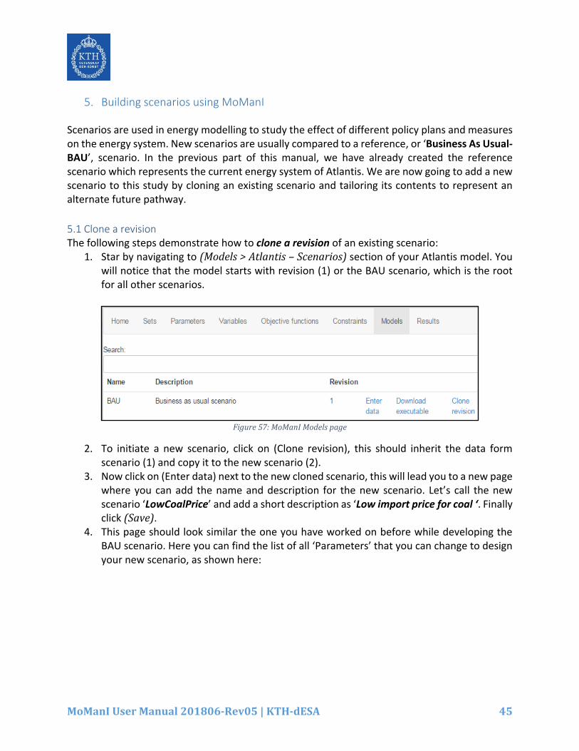
1. Star by navigating to (Models > Atlantis – Scenarios) section of your Atlantis model. You will notice that the model starts with revision (1) or the BAU scenario, which is the root for all other scenarios.

Figure 57: MoManI Models page

2. To initiate a new scenario, click on (Clone revision), this should inherit the data form scenario (1) and copy it to the new scenario (2).

3. Now click on (Enter data) next to the new cloned scenario, this will lead you to a new page where you can add the name and description for the new scenario. Let’s call the new scenario ‘LowCoalPrice’ and add a short description as ‘Low import price for coal ‘. Finally click (Save).

4. This page should look similar the one you have worked on before while developing the BAU scenario. Here you can find the list of all ‘Parameters’ that you can change to design your new scenario, as shown here:


Figure 58 : Entering Scenario data page showing list of Sets and Parameters

5.2 Developing a new scenario

Each scenario has its special characteristics. These are implemented by changing the input data for different parameter (s) in each scenario. In this example, and for the sake of simplicity, you will develop a scenario where only one parameter is adjusted or changed. In other more complicated cases, more than one parameter need to be changed to develop a scenario. As mentioned above, for Atlantis we would like to study the effect of a reduced import price for coal: how would this change the energy system of Atlantis? To implement this,

1. First, locate the VariableCost parameter and click on (Enter Data). Fix the Region as (Atlantis) and the mode of operation as (1) to allow MoManI to generate a table of Technologies as rows and years as columns.

2. Change the variable cost of (CO_IMP) to 1 throughout the time frame of the model. See Figure 59.

3. Click (Save) to implement the changes. This will take you back to the “Entering scenario data” page.

4. Go all the way to the bottom of the page and click on “Back to scenario list”. This should take you back to the Atlantis model page where you have the list of all the scenarios. So far we have created scenarios (1) and (2), the same approach can be implemented to add as many scenarios as you need.


Figure 59: Change data for variable cost for CO_IMP for years 2014 - 2040


6. Run Simulation

After developing two scenarios (BAU and LowCoalPrice), we are ready to run the simulation and see the results. MoManI is the interface that generates the required model and data files. In order to run the model and upload results to MoManI however, we need to download the GLPK solver.

Figure 60: Schematic representation on running simulation using MoManI and GLPK

1. After generating the model, the next step is to set up the solver that is used for running the optimization. In this example, GLPK solver is used to run the optimization, which is an open source free solver. If you don’t have this solver in your computer, follow the installation instructions given in Appendix 1 .

2. Once the solver is successfully installed, go back to MoManI, navigate to (Models > Atlantis – Scenarios > LowCoalPrice) and click on “Download executable”.

Figure 61: Downloading executable file from MoManI

3. Open the downloaded zip folder, you will find three text files named as (data.txt, metadata.txt and model.txt) and an executable file. Double click on the executable file “RunSimulation.exe”, this will open a new window, click on Run. Note that you may need


to un-zip the folder and move the content to another folder before you click on RunSimulation.exe

Figure 62: Run simulation

This should run the new scenario. Two separate screens will appear and you can see that simulation is running to find the optimal solution for the given model configuration. If the optimal solution cannot be found, you should see an error message on this screen.

Figure 63: Running simulation with GLPK solver

Once the simulation is finished and the optimal solution is found, the solver will upload results back to MoManI. It will also generate a folder called (res) with all result outputs in excel format (.csv) to be used in further analyses.


7. Results Visualization

Easy and fast presentation of results is an important aspect in the development of energy planning tools. This section in MoManI reduces analysis time considerably by providing a visualization screen for optimisation outputs in both graphical and tabular representation. From the top tabs, click on (Results) to go the results page where you can see on the left side a list of all models that have been developed (In this case we have only Atlantis). On the right side you have two options to visualize results a) View scenarios and b) Compare results as shown:

Figure 64: Results page showing Atlantis scenarios

7.1 View Scenarios: This option allows users to visualize results of a specific scenario. Once you click on view scenarios, you will move to a new page where you will find to the left a list of the scenarios under the Atlantis model (BAU and LowCoalPrice). And to the right you can see a note; either (View results) which means that the run was successful and results were uploaded to the interface. Or in the other case; you will have (No results yet) to give you a warning that there was an issue in running the optimization and uploading results, as shown below:

Figure 65: List of scenarios under Atlantis model

1. Click on (View results) next to (BAU) to go to further detailed list showing all output results

(Variables) available for this scenario. This list of variable results (output) might reminds you of the list of parameters (input) entered for each scenario.


Figure 66: List of variable results (output) under the BAU scenario

2. To the right you can find two options of results visualization, either using the standard charts developed in MoManI (View charts) or if you would like to further analyse results and to develop your own set of charts, you can (Download csv) file for each variable for your further analysis. In this section, we will focus on the first option and visualize the charts developed by MoManI.

3. From the variables list, look up ProductionbyTechnologyAnnual and click on (View charts) next to this variable. This will open a new page with a chart as shown below:


Figure 67: Results visualization for variable Production by technology annual – Grouped by region

4. You can change the setting of the graph using: a) Changing the output of the x-axis; click on the drop down list and chose (Year). b) Changing the output of the y-axis; clink in the drop down list under ‘Group by’ and chose (Technology) to segregate the production per technology. Since we are interested in this task to look into the electricity generation technologies, we need to zoon in further. c) Click on ‘show additional settings’; then de-activate (show legends) to allow for a bigger chart space. Secondly from ‘Display data for’ select the first group ‘Electricity Generation’ and de-activate the other categories ‘import technologies’, ‘T & D’ and ‘ungrouped’. See Figure 68

Figure 68: Addtional Chart settings


5. Finally click on (Hide Settings), you can see the legends and the numerical values of

‘production by technology’ simply by putting the mouse pointer on the year of interest. Your chart should look like the following:

Figure 69: Results visualization for variable ‘Production by technology annual’ – BAU scenario


7.2 Compare Results: The second option to visualize results is the ‘Compare results’ option, which will allow the

user to quickly compare specific variable results between two scenarios.

1. From the top tabs, click on (Results) to go back to the main results page. On the right side you have two options to visualize results, click on ‘Compare results’.

Figure 70: Main results page showing Atlantis model

2. In the ‘Compare scenario’ page you can change the arrangement of the scenarios in

your screen. For now, we will keep the default arrangement to have the ‘BAU’

scenario to the left and the ‘LowCoalPrice’ scenario to the right.

3. Again we will look into the ‘Production by Technology Annual’, look it up from the

drop down list under ‘Variable’. Then you should set the x-axis as years and ‘Group

by’ – Technology.

4. As we did previously, click on ‘show additional settings’ and perform the following

changes;

a) De-activate (show legends) to allow for a bigger chart space.

b) Under ‘Display data for’ select the first group ‘Electricity Generation’ and de-activate

the other categories ‘import technologies’, ‘T & D’ and ‘ungrouped’.

c) Finally click on (Hide Settings). Your screen should look like this:


Figure 71: Compare results of two scenarios – BAU to the left and LowCoalPrice to the right


References [1] M. Howells, H. Rogner, N. Strachan, C. Heaps, H. Huntington, S. Kypreos, A. Hughes, S. Silveira, J. DeCarolis, M. Bazillian and A. Roehrl, “OSeMOSYS: The Open Source Energy Modeling System, An introduction to its ethos, structure and development,” Energy Policy, vol. 39, p. 5850–5870, 2011. [2] M. Welsch, M. Howells, M. Bazilian, J. DeCarolis, S. Hermann and H. Rogner, “Modelling elements of Smart Grids – Enhancing the OSeMOSYS (Open Source Energy Modelling System) code,” Energy, vol. Volume 46, no. Issue 1, p. Pages 337–350, October 2012. [3] ETSAP (Energy Technology Systems Analysis Program), Software and Tools, 2015. [Online]. Available: http://www.etsap.org/Tools.asp. [4] IAEA (International Atomic Energy Agency), PESS Energy Models, 2015. [Online]. Available: https://www.iaea.org/OurWork/ST/NE/Pess/PESSenergymodels.html. [5] NTUA (National Technical University of Athens), The PRIMES Energy, 2015. [Online]. Available: http://www.e3mlab.ntua.gr/manuals/PRIMsd.pdf. [6] E. Van der Voort, “The EFOM 12C energy supply model within the EC,” Omega, vol. 10, no. 5, p. 507 523, 1982. [7] Enerdata, “POLES: Prospective Outlook on Long Term Energy Systems,” 2015. [Online]. Available: http://www.enerdata.net/enerdatauk/solutions/energy-models/poles-model.php.

http://www.etsap.org/Tools.asp

https://www.iaea.org/OurWork/ST/NE/Pess/PESSenergymodels.html

http://www.e3mlab.ntua.gr/manuals/PRIMsd.pdf

http://www.enerdata.net/enerdatauk/solutions/energy-models/poles-model.php


Appendix 1

GLPK installation guide for windows 10 users This instruction sheet is prepared for the training sessions on MoManI. In order to be able to use this effectively, you will need to have a computer with windows 10 as operating system and to have full administrative rights to be able to install and add new files to your system. Instructions:

1) First of all, you need to know the what is the type of your windows operating system.

To check that, navigate to: Control panel >> System >> About

2) Download the latest version of GLPK solver (glpk-4.60.tar.gz) from the following

link:

https://sourceforge.net/projects/winglpk/ This will download a zip file in your ‘downloads’ folder.

3) Extract the Zip folder by: right clicking on the folder and then>> 7-Zip >> Extract

Here as shown below:

https://sourceforge.net/projects/winglpk/


4) Now you will see a new folder called (glpk-4.60), move this folder to your (C: ) Drive

or any other folder you want the solver to be saved in. (Hint: You may need to log in

as administrator to be able to add a file to your C: drive.)

By this you have the solver installed in your computer, you DO NOT need to click install or run any executable. The only thing we need to be able to use the solver, is to set the environmental path variable. Which we will show in the following steps.

5) Double click on (glpk-4.60) folder, you should find many folders and files and

among them you can find two folders (w32) and (w64).

6) Based on the operating system type (step 1), open the (w32) folder if you have a 32-

bit operating system or open (w64) if you have a 64-bit operating system. In this

case we have 64-bit operating system and we open (w64).

7) From the address bar, COPY the directory to this folder (C:\glpk-4.60\w64) as

shown below:


8) On the right side of the browsing windows, right click on (This PC) and select

(Properties):

9) This will open a new window, on the right side menu, click on (Advanced System

Settings)

10) On this new window, click on (Environmental Variable) option at the bottom


11) Again you will have a new window. From bottom list, select (Path) and then click on

(Edit) as shown below:


12) This will lead you to a new window with a list of all path variable defined in your

computer, click on (New) to be able to add a new path variable to GLPK solver.

13) In the bottom field, paste the directory to GLPK (‘C:\glpk-4.60\w64’, which we have

copied in step 7):

Finally click (OK) to save your work.

To check if the solver is installed successfully:

1) Open (command prompt) window

2) Type (glpsol)

3) Click enter

4) You should find a msg like the one shown below: (GLPSOL: GLPK LP/MIP

Solver, v4-60):

momani user manual 201806-rev05 · 2018-05-30 · momani user manual 201806-rev05 | kth-desa 1 1...

Documents