Momentum Crashes

Kent Daniel and Tobias J. Moskowitz∗

Preliminary Draft: February 10, 2011

This Draft: June 16, 2015

- Abstract -

Despite their strong positive average returns across numerous asset classes, mo-mentum strategies can experience infrequent and persistent strings of negativereturns. These momentum crashes are partly forecastable. They occur in “panic”states – following market declines and when market volatility is high – and are con-temporaneous with market rebounds. The low ex ante expected returns in panicstates are consistent with a conditionally high premium attached to the option-like payoffs of past losers. An implementable dynamic momentum strategy basedon forecasts of momentum’s mean and variance approximately doubles the alphaand Sharpe Ratio of a static momentum strategy, and is not explained by otherfactors. These results are robust across multiple time periods, international equitymarkets, and other asset classes.

∗Columbia Business School and NBER, and Booth School of Business, University of Chicago and NBER,respectively. Contact information: kd2371@columbia.edu and Tobias.Moskowitz@chicagobooth.edu. For helpfulcomments and discussions we thank an anonymous referee, the editor Bill Schwert and Cliff Asness, JohnCochrane, Pierre Collin-Dufresne, Eugene Fama, Andrea Frazzini, Will Goetzmann, Gur Huberman, RonenIsrael, Narasimhan Jegadeesh, Mike Johannes, John Liew, Spencer Martin, Lasse Pedersen, Tano Santos, PaulTetlock, Sheridan Titman, and participants of the NBER Asset Pricing Summer Institute, the AFA meetings,the Quantitative Trading & Asset Management Conference at Columbia, the 5-Star Conference at NYU, andseminars at Columbia, Rutgers, University of Texas at Austin, USC, Yale, Aalto, BI Norwegian BusinessSchool, Copenhagen Business School, EPFL, McGill, Rice, Purdue, Baruch, Tulane, UCSD, the New YorkFed, Temple, the Swiss Finance Institute, Minnesota, the Q Group, Kepos Capital, and SAC. Moskowitz hasan ongoing relationship with AQR Capital which invests in, among many other things, momentum strategies.

1. Introduction

A momentum strategy is a bet on past returns predicting the cross-section of future returns,

typically implemented by buying past winners and selling past losers. Momentum is pervasive:

the academic literature documents the efficacy of momentum strategies across multiple time

periods, many markets, and in numerous asset classes.1

However, the strong positive average returns and Sharpe ratios of momentum strategies are

punctuated with occasional “crashes.” Like the returns to the carry trade in currencies (e.g.,

Brunnermeier, Nagel, and Pedersen (2008)), momentum returns are negatively skewed, and

the negative returns can be pronounced and persistent. In our 1927 to 2013 U.S. equity sample,

the two worst months for a momentum strategy that buys the top decile of past 12-month

winners and shorts the bottom decile of losers are consecutive: July and August of 1932. Over

this short period, the past-loser decile portfolio returned 232%, while the past-winner decile

portfolio had a gain of only 32%. In a more recent crash, over the three-month period from

March to May of 2009, the past-loser decile rose by 163%, while the decile portfolio of past

winners gained only 8%.

We investigate the impact and potential predictability of these momentum crashes, which

appear to be a key and robust feature of momentum strategies. We find that crashes tend to

occur in times of market stress, when the market has fallen and ex ante measures of volatility

are high, coupled with an abrupt rise in contemporaneous market returns.

Our result is consistent with that of Cooper, Gutierrez, and Hameed (2004) and Stivers and

Sun (2010), who find, respectively, that the momentum premium falls when the past three-

year market return has been negative and that the momentum premium is low when market

1Momentum strategies were first documented in U.S. common stock returns from 1965 to 1989 by Jegadeeshand Titman (1993) and Asness (1994), by sorting firms on the basis of three to 12 month past returns.Subsequently, Jegadeesh and Titman (2001) show the continuing efficacy of US equity momentum portfoliosin common stock returns in the 1990 to 1998 period. Israel and Moskowitz (2013) show the robustness ofmomentum prior to and after these studies from 1927 to 1965 and from 1990 to 2012. There is evidenceof momentum going back to the Victorian age from Chabot, Remy, and Jagannathan (2009) and evidencefrom 1801 to 2012 from Geczy and Samonov (2013) in what the authors call “the world’s longest backtest.”Moskowitz and Grinblatt (1999) find momentum in industry portfolios. Rouwenhorst (1998) and Rouwenhorst(1999) finds momentum in developed and emerging equity markets, respectively. Asness, Liew, and Stevens(1997) find momentum in country indices. Okunev and White (2003) find momentum in currencies; Erb andHarvey (2006) in commodities; Moskowitz, Ooi, and Pedersen (2012) in exchange traded futures contracts;and Asness, Moskowitz, and Pedersen (2013), who integrate this evidence across markets and asset classes,find momentum in bonds as well.

1

volatility is high. Cooper, Gutierrez, and Hameed (2004) offer a behavioral explanation for

these facts that may also be consistent with momentum performing particularly poorly during

market rebounds if those are also times when assets become more mispriced. However, we

investigate another source for these crashes by examining conditional risk measures.

In particular, the patterns we find are suggestive of the changing beta of the momentum

portfolio partly driving the momentum crashes. The time variation in betas of return-sorted

portfolios was first documented by Kothari and Shanken (1992), who argue that, by their

nature, past-return sorted portfolios will have significant time-varying exposure to systematic

factors. Because momentum strategies are long/overweight (short/underweight) past winners

(losers), they will have positive loadings on factors which have had a positive realization, and

negative loadings on factors which have had negative realizations, over the formation period

of the momentum strategy.

Grundy and Martin (2001) apply Kothari and Shanken’s insights to price momentum strate-

gies. Intuitively, the result is straightforward, if not often appreciated: when the market has

fallen significantly over the momentum formation period – in our case from 12 months ago to

one month ago – there is a good chance that the firms that fell in tandem with the market

were and are high beta firms, and those that performed the best were low beta firms. Thus,

following market declines, the momentum portfolio is likely to be long low-beta stocks (the

past winners), and short high-beta stocks (the past losers). We verify empirically that there is

dramatic time variation in the betas of momentum portfolios. We find that, following major

market declines, betas for the past-loser decile can rise above 3, and fall below 0.5 for past

winners. Hence, when the market rebounds quickly, momentum strategies will crash because

they have a conditionally large negative beta.

Grundy and Martin (2001) argue that performance of momentum strategies is dramatically

improved, particularly in the pre-WWII era, by dynamically hedging market and size risk.

However, their hedged portfolio is constructed based on forward-looking betas, and is therefore

not an implementable strategy. We show that this results in a strong bias in estimated

returns, and that a hedging strategy based on ex ante betas does not exhibit the performance

improvement noted in Grundy and Martin (2001).

The source of the bias is a striking correlation of the loser-portfolio beta with the contem-

poraneous return on the market. Using a Henriksson and Merton (1981) specification, we

2

calculate up- and down-betas for the momentum portfolios and show that, in a bear market,

a momentum portfolio’s up-market beta is more than double its down-market beta (−1.51

versus −0.70 with a t-stat of the difference = 4.5). Outside of bear markets, there is no

statistically reliable difference in betas.

More detailed analysis reveals that most of the up- versus down-beta asymmetry in bear

markets is driven by the past losers. This pattern in dynamic betas of the loser portfolio

implies that momentum strategies in bear markets behave like written call options on the

market – when the market falls, they gain a little, but when the market rises they lose a lot.

Consistent with the written call option-like behavior of the momentum strategy in bear mar-

kets, we show that the momentum premium is correlated with the strategy’s time-varying

exposure to volatility risk. Using VIX-imputed variance-swap returns, we find that the mo-

mentum strategy payoff has a strong negative exposure to innovations in market variance in

bear markets, but not in normal (“bull”) markets. However, we also show that hedging out

this time varying exposure to market variance (by buying S&P variance swaps in bear mar-

kets, for instance) does not restore the profitability of momentum in bear markets. Hence,

time varying exposure to volatility risk does not explain the time variation in the momentum

premium.

Using the insights developed about the forecastability of momentum payoffs, and the fact that

the momentum strategy volatility is itself predictable and distinct from the predictability in its

mean return, we design an optimal dynamic momentum strategy in which the WML portfolio

is levered up or down over time so as to maximize the unconditional Sharpe ratio of the

portfolio. We first show theoretically that, to maximize the unconditional Sharpe ratio, a

dynamic strategy should scale the WML weight at each point in time so that the dynamic

strategy’s conditional volatility is proportional to the conditional Sharpe ratio of the strategy.

This insight comes directly from an intertemporal version of the standard Markowitz (1952)

optimization problem. Then, using the results from our analysis on the forecastability of both

the momentum premium and momentum volatility, we estimate these conditional moments

to generate the dynamic weights.

We find that the optimal dynamic strategy significantly outperforms the standard static mo-

mentum strategy, more than doubling its Sharpe ratio and delivering significant positive alpha

relative to the market, Fama and French factors, the static momentum portfolio and condi-

3

tional versions of all of these models that allow betas to vary in the crash states. In addition,

the dynamic momentum strategy also significantly outperforms constant volatility momen-

tum strategies suggested in the literature (e.g., Barroso and Santa-Clara (2012)), producing

positive alpha relative to the constant volatility strategy and capturing the constant volatility

strategy’s returns in spanning tests. The dynamic strategy not only helps smooth the volatil-

ity of momentum portfolios, as does the constant volatility approach, but in addition also

exploits the strong forecastability of the momentum premium.

Given the paucity of momentum crashes and the pernicious effects of data mining from an

ever-expanding search across studies (and in practice) for strategies that improve performance,

we challenge the robustness of our findings by replicating the results in different sample peri-

ods, four different equity markets, and five distinct asset classes. Across different time periods,

markets, and asset classes, we find remarkably consistent results. First, the results are robust

in every quarter-century subsample in US equities. Second, we show that momentum strate-

gies in all markets and asset classes suffer from crashes, which are consistently driven by the

conditional beta and option-like feature of losers. The same option-like behavior of losers in

bear markets is present in Europe, Japan, the UK, globally, and is a feature of index futures-,

commodity-, fixed income-, and currency-momentum strategies. Third, the same dynamic

momentum strategy applied in these alternative markets and asset classes is ubiquitously suc-

cessful in generating superior performance over the static and constant volatility momentum

strategies in each market and asset class. The additional improvement from dynamic weight-

ing is large enough to produce significant momentum profits even in markets where the static

momentum strategy has famously failed to yield positive profits – e.g., Japan. Taken together,

and applied across all markets and asset classes, an implementable dynamic momentum strat-

egy delivers an annualized Sharpe ratio of 1.19, which is four times larger than that of the

static momentum strategy applied to US equities over the same period, and thus posing an

even greater challenge for rational asset pricing models (Hansen and Jagannathan, 1991).

Finally, we consider several possible explanations for the option-like behavior of momentum

payoffs, particularly for losers. For equity momentum strategies, one possibility is that the

optionality arises because a share of common stock is a call option on the underlying firm’s

assets when there is debt in the capital structure (Merton, 1974). Particularly in distressed

periods where this option-like behavior is manifested, the underlying firm values among past

losers have generally suffered severely, and are therefore potentially much closer to a level

where the option convexity is strong. The past winners, in contrast, would not have suffered

4

the same losses, and may still be “in-the-money.” While this explanation seems to have merit

for equity momentum portfolios, this hypothesis does not seem applicable for index future,

commodity, fixed income, and currency momentum, which also exhibit option-like behavior.

In the conclusion, we briefly discuss a behaviorally motivated possible explanation for these

option-like features that could apply to all asset classes, but a fuller understanding of these

convex payoffs is an open area for future research.

The layout of the paper is as follows: Section 2 describes the data and portfolio construction

and dissects momentum crashes in US equities. Section 3 measures the conditional betas and

option-like payoffs of losers and assesses to what extent these crashes are predictable based

on these insights. Section 4 examines the performance of an optimal dynamic strategy based

on our findings, and whether its performance can be explained by dynamic loadings on other

known factors or other momentum strategies proposed in the literature. Section 5 examines

the robustness of our findings in different time periods, international equity markets, and

other asset classes. Section 6 concludes by speculating about the sources of the premia we

observe and discusses areas for future research.

2. US equity momentum

In this section, we present the results of our analysis of momentum in US common stocks over

the 1927 to 2013 time period. We begin with the data description and portfolio construction.

2.1. US equity data and momentum portfolio construction

Our principal data source is the Center for Research in Security Prices (CRSP). We construct

monthly and daily momentum decile portfolios, where both sets of portfolios are rebalanced

at the end of each month. The universe starts with all firms listed on NYSE, AMEX or

NASDAQ as of the formation date, using only the returns of common shares (with CRSP

sharecode of 10 or 11). We require that a firm have a valid share price and number of shares

as of the formation date, and that there be a minimum of eight monthly returns over the

past 11 months, skipping the most recent month, which is our formation period. Following

convention and CRSP availability, all prices are closing prices, and all returns are from close

to close.

5

To form the momentum portfolios, we first rank stocks based on their cumulative returns

from 12 months before to one month before the formation date (i.e., the t− 12 to t− 2-month

returns), where, consistent with the literature (Jegadeesh and Titman, 1993, Asness, 1994,

Fama and French, 1996), we use a one month gap between the end of the ranking period and

the start of the holding period to avoid the short-term reversals documented by Jegadeesh

(1990) and Lehmann (1990). All firms meeting the data requirements are then placed into

one of ten decile portfolios based on this ranking, where portfolio 10 represents the “Winners”

(those with the highest past returns) and portfolio 1 the “Losers.” The value-weighted holding

period returns of the decile portfolios are computed, where portfolio membership does not

change within a month except in the case of delisting.2

The market return is the value weighted index of all listed firms in CRSP and the risk free

rate series is the one-month Treasury bill rate, both obtained from Ken French’s data library.

We convert the monthly risk-free rate series to a daily series by converting the risk-free rate

at the beginning of each month to a daily rate, and assuming that that daily rate is valid

throughout the month.

2.2. Momentum portfolio performance

Figure 1 presents the cumulative monthly returns from 1927:01-2013:03 for investments in:

(1) the risk-free asset; (2) the market portfolio; (3) the bottom decile “past loser” portfolio;

and (4) the top decile “past winner” portfolio. On the right side of the plot, we present the

final dollar values for each of the four portfolios, given a $1 investment in January, 1927 (and,

of course, assuming no transaction costs).

Consistent with the existing literature, there is a strong momentum premium over the last

century. The winners significantly outperform the losers and by much more than equities

have outperformed Treasuries. Table 1 presents return moments for the momentum decile

portfolios over this period. The winner decile excess return averages 15.3% per year, and the

loser portfolio averages −2.5% per year. In contrast the average excess market return is 7.6%.

The Sharpe ratio of the WML portfolio is 0.71, and that of the market is 0.40. Over this

period, the beta of the WML portfolio is negative, −0.58, giving it an unconditional CAPM

alpha of 22.3% per year (t-stat = 8.5). Consistent with the high alpha, an ex post optimal

2Daily and Monthly returns to these portfolios, and additional details on their construction are availableat Kent Daniel’s website: http://www.kentdaniel.net/data.php.

6

Fig. 1. Winners and Losers, 1927-2013. Plotted are the cumulative returns to four assets: (1) therisk-free asset; (2) the CRSP value-weighted index; (3) the bottom decile “past loser” portfolio; and(4) the top decile “past winner” portfolio over the full sample period 1927:01 to 2013:03. To the rightof the plot we tabulate the final dollar values for each of the four portfolios, given a $1 investmentin January 1927.

combination of the market and WML portfolio has a Sharpe ratio more than double that of

the market.

2.3. Momentum crashes

The momentum strategy’s average returns are large and highly statistically significant, but

since 1927 there have been a number of long periods over which momentum under-performed

dramatically. Figure 1 highlights two momentum “crashes” in particular: June 1932 to De-

cember 1939 and more recently March 2009 to March 2013. These two periods represent the

two largest sustained drawdown periods for the momentum strategy and are selected pur-

posely to illustrate the crashes we study more generally in this paper. The starting dates for

these two periods are not selected randomly: March 2009 and June 1932 are, respectively,

the “market bottoms” following the stock market decline associated with the recent financial

crisis, and with the market decline from the great depression.

Zeroing in on these crash periods, Figure 2 shows the cumulative daily returns to the same

7

Table 1Momentum portfolio characteristics, 1927:01-2013:03This table presents characteristics of the monthly momentum decile portfolio excess returns over the87 year full sample period from 1927:01-2013:03. Decile 1 represents the biggest losers and decile 10the biggest winners, with WML representing the zero-cost winners minus losers portfolio. The meanexcess return, standard deviation, and alpha are in percent, and annualized. The Sharpe ratio isannualized. The α, t(α), and β are estimated from a full-period regression of each decile portfolio’sexcess return on the excess CRSP-value weighted index. For all portfolios except WML, sk(m)denotes the full-period realized skewness of the monthly log returns (not excess) to the portfoliosand sk(d) denotes the full-period realized skewness of the daily log returns. For WML, sk is therealized skewness of log(1+rWML+rf ).

Momentum Decile Portfolios1 2 3 4 5 6 7 8 9 10 wml Mkt

r − rf -2.5 2.9 2.9 6.4 7.1 7.1 9.2 10.4 11.3 15.3 17.9 7.7σ 36.5 30.5 25.9 23.2 21.3 20.2 19.5 19.0 20.3 23.7 30.0 18.8α -14.7 -7.8 -6.4 -2.1 -0.9 -0.6 1.8 3.2 3.8 7.5 22.2 0t(α) (-6.7) (-4.7) (-5.3) (-2.1) (-1.1) (-1.0) (2.8) (4.5) (4.3) (5.1) (7.3) (0)β 1.61 1.41 1.23 1.13 1.05 1.02 0.98 0.95 0.99 1.03 -0.58 1SR -0.07 0.09 0.11 0.28 0.33 0.35 0.47 0.54 0.56 0.65 0.60 0.41sk(m) 0.09 -0.05 -0.19 0.21 -0.13 -0.30 -0.55 -0.54 -0.76 -0.82 -4.70 -0.57sk(d) 0.12 0.29 0.22 0.27 0.10 -0.10 -0.44 -0.66 -0.67 -0.61 -1.18 -0.44

set of portfolios from Figure 1 – risk-free, market, past losers, past winners – over these

subsamples. Over both of these periods, the loser portfolio strongly outperforms the winner

portfolio. From March 8, 2009 to March 28, 2013, the losers produce more than twice the

profits of the winners, which also underperform the market over this period. From June 1,

1932 to December 30, 1939 the losers outperform the winners by 50%.

Table 1 also shows that the winner portfolios are considerably more negatively skewed (monthly

and daily) than the loser portfolios. While the winners still outperform the losers over time,

the Sharpe ratio and alpha understate the significance of these crashes. Looking at the skew-

ness of the portfolios, winners become more negatively skewed moving to more extreme deciles.

For the top winner decile portfolio, the monthly (daily) skewness is -0.82 (-0.61), while for the

most extreme bottom decile of losers the skewness is 0.09 (0.12). The WML portfolio over

this full sample period has a monthly (daily) skewness of -4.70 (-1.18).

Table 2 presents the worst monthly returns to the WML strategy, as well as the lagged two-

year returns on the market and the contemporaneous monthly market return. Several key

points emerge from Table 2 as well as from Figures 1 and 2:

8

Aug 2009 Feb 2010 Aug 2010 Feb 2011 Aug 2011 Feb 2012 Aug 2012 Feb 2013date

1

2

3

4

5

6

($ v

alu

e o

f in

vest

ment)

Cumulative Gains from Investments, Mar 09, 2009 - Mar 28, 2013

risk-freemarketpast loserspast winners

1933 1934 1935 1936 1937 1938 1939date

1

2

3

4

5

6

($ v

alu

e o

f in

vest

ment)

Cumulative Gains from Investments, Jun 01, 1932 - Dec 30, 1939

risk-freemarketpast loserspast winners

Fig. 2. Momentum crashes, following the great depression and the 2008-09 financial crisis. Theseplots show the cumulative daily returns to four portfolios: (1) the risk-free asset; (2) the CRSP value-weighted index; (3) the bottom decile “past loser” portfolio; and (4) the top decile “past winner”portfolio over the period from March 9, 2009 through March, 28 2013 (top graph) and from June 1,1932 through December 30, 1939 (bottom graph).

9

1. While past winners have generally outperformed past losers, there are relatively longperiods over which momentum experiences severe losses or “crashes.”

2. Fourteen of the 15 worst momentum returns occur when the lagged two-year marketreturn is negative. All occur in months where the market rose contemporaneously, oftenin a dramatic fashion.

3. The clustering evident in both this table and in the daily cumulative returns in Figure2 make it clear that the crashes have relatively long duration. They do not occur overthe span of minutes or days – a crash is not a Poisson jump. They take place slowly,over the span of multiple months.

4. Similarly, the extreme losses are clustered: The two worst months for momentum areback-to-back, in July and August of 1932, following a market decline of roughly 90%from the 1929 peak. March and April of 2009 are the 7th and 4th worst momentummonths, respectively, and April and May of 1933 are the 6th and 12th worst. Three ofthe ten worst momentum monthly returns are from 2009 – a three-month period in whichthe market rose dramatically and volatility fell. While it might not seem surprising thatthe most extreme returns occur in periods of high volatility, the effect is asymmetric forlosses versus gains: the extreme momentum gains are not nearly as large in magnitude,nor as concentrated in time.

5. Closer examination reveals that the crash performance is mostly attributable to the shortside or the performance of losers. For example, in July and August of 1932, the marketactually rose by 82%. Over these two months, the winner decile rose by 32%, but theloser decile was up by 232%. Similarly, over the three month period from March to Mayof 2009, the market was up by 26%, but the loser decile was up by 163%. Thus, to theextent that the strong momentum reversals we observe in the data can be characterizedas a crash, they are a crash where the short side of the portfolio – the losers – are“crashing up” rather than down.

Table 2 also suggests that large changes in market beta may help to explain some of the

large negative returns earned by momentum strategies. For example, as of the beginning of

March 2009, the firms in the loser decile portfolio were, on average, down from their peak

by 84%. These firms included those hit hardest by the financial crisis: Citigroup, Bank of

America, Ford, GM, and International Paper (which was highly levered). In contrast, the

past-winner portfolio was composed of defensive or counter-cyclical firms like Autozone. The

loser firms, in particular, were often extremely levered, and at risk of bankruptcy. In the sense

of the Merton (1974) model, their common stock was effectively an out-of-the-money option

on the underlying firm value. This suggests that there were potentially large differences in

the market betas of the winner and loser portfolios that generate convex, option-like payoffs

– a conjecture we now investigate more formally in the next section.

10

Table 2Worst monthly momentum returnsThis table lists the 15 worst monthly returns to the WML momentum portfolio over the 1927:01-2013:03 time period. Also tabulated are Mkt-2y, the 2-year market returns leading up to the portfolioformation date, and Mktt, the contemporaneous market return. The dates between July 1932 andSeptember 1939 are marked with ∗, those between April and August of 2009 with †; those fromJanuary 2001 and November 2002 with ‡. All numbers in the table are in percent.

Rank Month WMLt MKT-2y Mktt1 1932-08∗ -74.36 -67.77 36.492 1932-07∗ -60.98 -74.91 33.633 2001-01‡ -49.19 10.74 3.664 2009-04† -45.52 -40.62 10.205 1939-09∗ -43.83 -21.46 16.976 1933-04∗ -43.14 -59.00 38.147 2009-03† -42.28 -44.90 8.978 2002-11‡ -37.04 -36.23 6.089 1938-06∗ -33.36 -27.83 23.7210 2009-08† -30.54 -27.33 3.3311 1931-06∗ -29.72 -47.59 13.8712 1933-05∗ -28.90 -37.18 21.4213 2001-11‡ -25.31 -19.77 7.7114 2001-10‡ -24.98 -16.77 2.6815 1974-01 -24.04 -5.67 0.46

3. Time-varying beta and option-like payoffs

To investigate the time-varying betas of winners and losers, Figure 3 plots the market betas for

the winner and loser momentum deciles, estimated using 126 day (≈ 6 month) rolling market

model regressions with daily data.3 Figure 3 plots the betas over three non-overlapping

subsamples that span the full sample period: June 1927 to December 1939, January 1940 to

December 1999, and January 2000 to March 2013.

3We use 10 daily lags of the market return in estimating the market betas. Specifically, we estimate a dailyregression specification of the form:

rei,t = β0rem,t + β1r

em,t−1 + · · ·+ β10r

em,t−10 + εi,t

and then report the sum of the estimated coefficients β0 + β1 + · · · + β10. Particularly for the past loserportfolios, and especially in the pre-WWII period, the lagged coefficients are strongly significant, suggestingthat market wide information is incorporated into the prices of many of the firms in these portfolios over thespan of multiple days. See Lo and MacKinlay (1990) and Jegadeesh and Titman (1995).

11

19281930

19321934

19361938

0.0

0.5

1.0

1.5

2.0

2.5

3.0

3.5

4.0

126 d

ay (

rolli

ng)

beta

1927:06 - 1939:12

loser decilewinner decile

19501960

19701980

19900.0

0.5

1.0

1.5

2.0

2.5

3.0

126 d

ay (

rolli

ng)

beta

1940:01 - 1999:12

20022004

20062008

20102012

date

0

1

2

3

4

5

126 d

ay (

rolli

ng)

beta

2000:01 - 2013:03

Fig. 3. Market betas of winner and loser decile portfolios. These three plots present the estimatedmarket betas over three independent subsamples spanning our full sample: 1927:06 to 1939:12,1940:01 to 1999:12, and 2000:01 to 2013:03. The betas are estimated by running a set of 126-dayrolling regressions of the momentum portfolio excess returns on the contemporaneous excess marketreturn and 10 (daily) lags of the market return, and summing the betas.

12

The betas vary substantially, especially for the loser portfolio, whose beta tends to increase

dramatically during volatile periods. The first and third plots highlight the betas several

years before, during, and after the momentum crashes. The beta of the winner portfolio is

sometimes above 2 following large market rises, but for the loser portfolio, the beta reaches far

higher levels (as high as 4 or 5). The widening beta differences between winners and losers,

coupled with the facts from Table 2 that these crash periods are characterized by sudden and

dramatic market upswings, means that the WML strategy will experience huge losses during

these times. We examine these patterns more formally by investigating how the mean return

of the momentum portfolio is linked to time variation in market beta.

3.1. Hedging market risk in the momentum portfolio

Grundy and Martin (2001) explore this same question, arguing that the poor performance of

the momentum portfolio in the pre-WWII period first documented by Jegadeesh and Titman

(1993) is a result of time varying market and size exposure. Specifically, they argue that a

hedged momentum portfolio – for which conditional market and size exposure is zero – has

a high average return and a high Sharpe-ratio in the pre-WWII period when the unhedged

momentum portfolio suffers.

At the time that Grundy and Martin (2001) undertook their study, daily stock return data

was not available through CRSP in the pre-1962 period. Given the dynamic nature of mo-

mentum’s risk-exposures, estimating the future hedge coefficients ex ante with monthly data

is problematic. As a result, Grundy and Martin (2001) use an ex post estimate of the portfo-

lio’s market and size betas using monthly returns over the current month and the future five

months.

However, to the extent that the future momentum-portfolio beta is correlated with the future

return of the market, this procedure will result in a biased estimate of the returns of the

hedged portfolio. We show there is in fact a strong correlation of this type, which results in

a large upward bias in the estimated performance of the hedged portfolio.4

4The result that the betas of winner-minus-loser portfolios are non-linearly related to contemporaneousmarket returns has also been documented in Rouwenhorst (1998) who documents this feature for non-USequity momentum strategies (Table V, p. 279). Chan (1988) and DeBondt and Thaler (1987) document thisnon-linearity for longer-term winner/loser portfolios. However, Boguth, Carlson, Fisher, and Simutin (2010),building on the results of Jagannathan and Korajczyk (1986), note that the interpretation of the measures ofabnormal performance (i.e., the alphas) in Chan (1988), Grundy and Martin (2001), and Rouwenhorst (1998)

13

Table 3Market timing regression resultsThis table presents the results of estimating four specifications of a monthly time-series regressionsrun over the period 1927:01 to 2013:03. In all cases the dependent variable is the return on theWML portfolio. The independent variables are a constant, an indicator for bear markets, IB,t−1,which equals one if the cumulative past two-year return on the market is negative, the excess marketreturn, Rem,t, and a contemporaneous up-market indicator, IU,t, which equals one if Rem,t > 0. Thecoefficients α0 and αB are ×100 (i.e., are in percent per month).

Estimated Coefficients(t-statistics in parentheses)

Coef. Variable (1) (2) (3) (4)α0 1 1.852 1.976 1.976 2.030

(7.3) (7.7) (7.8) (8.4)αB IB,t−1 -2.040 0.583

(-3.4) (0.7)

β0 Rem,t -0.576 -0.032 -0.032 -0.034

(-12.5) (-0.5) (-0.6) (-0.6)

βB IB,t−1 ·Rem,t -1.131 -0.661 -0.708

(-13.4) (-5.0) (-6.1)

βB,U IB,t−1·IU,t ·Rem,t -0.815 -0.727

(-4.5) (-5.6)R2adj 0.130 0.269 0.283 0.283

3.2. Option-like behavior of the WML portfolio

The source of the bias using ex post beta of the momentum portfolio to construct the hedge

portfolio is that, in bear markets, the market beta of the WML portfolio is strongly negatively

correlated with the contemporaneous realized market return. This means that the hedge

portfolio constructed based on the ex post beta will have a higher beta in anticipation of a

higher future market return, making its performance much better that what would be possible

with a hedge portfolio based on the ex ante beta.

In this section we also show that the return of the momentum portfolio, net of properly

estimated market risk, is significantly lower in bear markets. Both of these results are linked

to the fact that, in bear markets, the momentum strategy behaves as if it is effectively short

a call option on the market.

are problematic and provide a critique of Grundy and Martin (2001) and other studies which “overcondition”in a similar way.

14

We first illustrate these issues with a set of four monthly time-series regressions, the results

of which are presented in Table 3. The dependent variable in all regressions is RWML,t, the

WML return in month t. The independent variables are combinations of:

1. Rem,t, the CRSP value-weighted (VW) index excess return in month t.

2. IB,t−1, an ex ante bear-market indicator that equals 1 if the cumulative CRSP VW indexreturn in the past 24 months is negative, and is zero otherwise.

3. IU,t, a the contemporaneous – i.e., not ex ante – up-market indicator variable. It is 1 ifthe excess CRSP VW index return is greater than the risk-free rate in month t (e.g.,Rem,t > 0), and is zero otherwise.5

Regression (1) in Table 3 fits an unconditional market model to the WML portfolio:

RWML,t = α0 + β0Rm,t + εt. (1)

Consistent with the results in the literature, the estimated market beta is negative, -0.576, and

the intercept, α, is both economically large (1.852% per month), and statistically significant

(t-stat = 7.3).

Regression (2) in Table 3 fits a conditional CAPM with the bear market indicator, IB, as an

instrument:

RWML,t = (α0 + αBIB,t−1) + (β0 + βBIB,t−1)Rm,t + εt. (2)

This specification is an attempt to capture both expected return and market-beta differences

in bear markets. First, consistent with Grundy and Martin (2001), we see a striking change

in the market beta of the WML portfolio in bear markets: it is -1.131 lower, with a t-statistic

of −13.4 on the difference. The WML alpha in bear is 2.04 %/month lower (t = −3.4) also

lower. Interestingly, the point estimate for the alpha in bear markets – equal to α0 + αB is

just below zero, but not statistically significant.

Regression (3) introduces an additional element to the regression which allows us to assess

the extent to which the up- and down-market betas of the WML portfolio differ:

RWML,t = [α0 + αB · IB,t−1] + [β0 + IB,t−1(βB + IU,tβB,U)]Rm,t + εt. (3)

5Of the 1,035 months in the 1927:01-2013:03 period, IB,t−1 = 1 in 183, and IU,t = 1 in 618.

15

This specification is similar to that used by Henriksson and Merton (1981) to assess market

timing ability of fund managers. Here, the βB,U of -0.815 (t = −4.5) shows that the WML

portfolio does very badly when the market “rebounds” following a bear market. Specifically,

when in a bear-market, the point estimates of the WML beta are −0.742 (= β0 + βB) when

the contemporaneous market return is negative, and = β0 + βB + βB,U = −1.796 when the

market return is positive. In other words, the momentum portfolio is effectively short a call

option on the market

The predominant source of this optionality comes from the loser portfolio. Panel A of Table 4

presents the results of the regression specification in equation (3) for each of the ten momentum

portfolios. The final row of the table (the βB,U coefficient) shows the strong up-market betas

for the loser portfolios in bear markets. For the loser decile, the down-market beta is 1.560

(= 1.338 + 0.222) and the point estimate of the up-market beta is 2.160 (= 1.560 + 0.600).

Also, note the slightly negative up-market beta increment for the winner decile (= −0.215).

This pattern also holds for less extreme winners and losers, such as decile 2 versus decile 9 or

decile 3 versus 8, with the differences between winners and losers declining monotonically for

less extreme past return sorted portfolios. The net effect is that a momentum portfolio which

is long winners and short losers will have significant negative market exposure following bear

markets precisely when the market swings upward, and that exposure is even more negative

for more extreme past return sorted portfolios.

3.3. Asymmetry in the optionality

The optionality associated with the loser portfolios is only significant in bear markets. Panel

B of Table 4 presents the same set of regressions using the bull-market indicator IL,t−1 instead

of the bear-market indicator IB,t−1. The key variables here are the estimated coefficients and

t-statistics on βL,U , presented in the last two rows of Panel B. Unlike in Panel A, there is no

significant asymmetry present in the loser portfolio, though the winner portfolio asymmetry

is comparable to Panel A. The net effect is that the WML portfolio shows no statistically

significant optionality in bull markets, unlike what we see in bear markets.

16

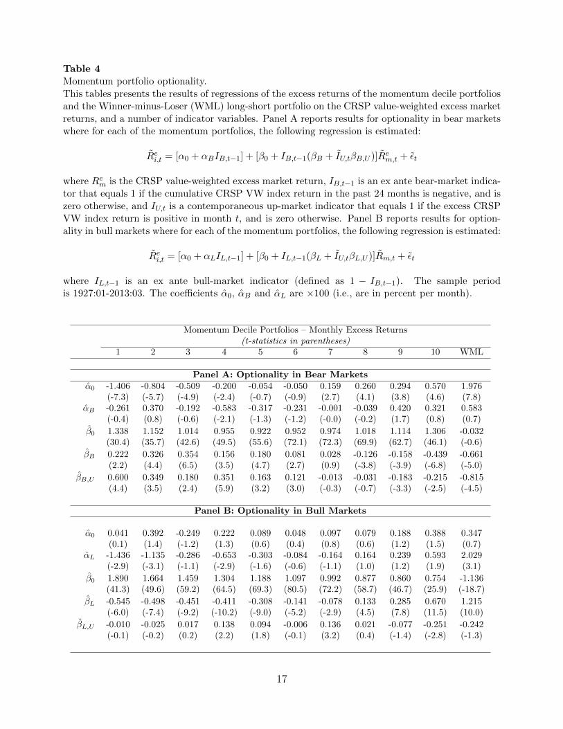
Table 4Momentum portfolio optionality.This tables presents the results of regressions of the excess returns of the momentum decile portfoliosand the Winner-minus-Loser (WML) long-short portfolio on the CRSP value-weighted excess marketreturns, and a number of indicator variables. Panel A reports results for optionality in bear marketswhere for each of the momentum portfolios, the following regression is estimated:

Rei,t = [α0 + αBIB,t−1] + [β0 + IB,t−1(βB + IU,tβB,U )]Rem,t + εt

where Rem is the CRSP value-weighted excess market return, IB,t−1 is an ex ante bear-market indica-tor that equals 1 if the cumulative CRSP VW index return in the past 24 months is negative, and iszero otherwise, and IU,t is a contemporaneous up-market indicator that equals 1 if the excess CRSPVW index return is positive in month t, and is zero otherwise. Panel B reports results for option-ality in bull markets where for each of the momentum portfolios, the following regression is estimated:

Rei,t = [α0 + αLIL,t−1] + [β0 + IL,t−1(βL + IU,tβL,U )]Rm,t + εt

where IL,t−1 is an ex ante bull-market indicator (defined as 1 − IB,t−1). The sample periodis 1927:01-2013:03. The coefficients α0, αB and αL are ×100 (i.e., are in percent per month).

Momentum Decile Portfolios – Monthly Excess Returns(t-statistics in parentheses)

1 2 3 4 5 6 7 8 9 10 WML

Panel A: Optionality in Bear Marketsα0 -1.406 -0.804 -0.509 -0.200 -0.054 -0.050 0.159 0.260 0.294 0.570 1.976

(-7.3) (-5.7) (-4.9) (-2.4) (-0.7) (-0.9) (2.7) (4.1) (3.8) (4.6) (7.8)αB -0.261 0.370 -0.192 -0.583 -0.317 -0.231 -0.001 -0.039 0.420 0.321 0.583

(-0.4) (0.8) (-0.6) (-2.1) (-1.3) (-1.2) (-0.0) (-0.2) (1.7) (0.8) (0.7)

β0 1.338 1.152 1.014 0.955 0.922 0.952 0.974 1.018 1.114 1.306 -0.032(30.4) (35.7) (42.6) (49.5) (55.6) (72.1) (72.3) (69.9) (62.7) (46.1) (-0.6)

βB 0.222 0.326 0.354 0.156 0.180 0.081 0.028 -0.126 -0.158 -0.439 -0.661(2.2) (4.4) (6.5) (3.5) (4.7) (2.7) (0.9) (-3.8) (-3.9) (-6.8) (-5.0)

βB,U 0.600 0.349 0.180 0.351 0.163 0.121 -0.013 -0.031 -0.183 -0.215 -0.815(4.4) (3.5) (2.4) (5.9) (3.2) (3.0) (-0.3) (-0.7) (-3.3) (-2.5) (-4.5)

Panel B: Optionality in Bull Markets

α0 0.041 0.392 -0.249 0.222 0.089 0.048 0.097 0.079 0.188 0.388 0.347(0.1) (1.4) (-1.2) (1.3) (0.6) (0.4) (0.8) (0.6) (1.2) (1.5) (0.7)

αL -1.436 -1.135 -0.286 -0.653 -0.303 -0.084 -0.164 0.164 0.239 0.593 2.029(-2.9) (-3.1) (-1.1) (-2.9) (-1.6) (-0.6) (-1.1) (1.0) (1.2) (1.9) (3.1)

β0 1.890 1.664 1.459 1.304 1.188 1.097 0.992 0.877 0.860 0.754 -1.136(41.3) (49.6) (59.2) (64.5) (69.3) (80.5) (72.2) (58.7) (46.7) (25.9) (-18.7)

βL -0.545 -0.498 -0.451 -0.411 -0.308 -0.141 -0.078 0.133 0.285 0.670 1.215(-6.0) (-7.4) (-9.2) (-10.2) (-9.0) (-5.2) (-2.9) (4.5) (7.8) (11.5) (10.0)

βL,U -0.010 -0.025 0.017 0.138 0.094 -0.006 0.136 0.021 -0.077 -0.251 -0.242(-0.1) (-0.2) (0.2) (2.2) (1.8) (-0.1) (3.2) (0.4) (-1.4) (-2.8) (-1.3)

17

19281930

19321934

19361938

date

100

101

port

folio

val

ue

Cumulative Daily Returns to Momentum Strategies, 1927:06-1939:12

unhedgedex-post hedgedex-ante hedged

19311941

19511961

19711981

19912001

2011

date

10-1

100

101

102

103

104

105

106

107

108

109

1010

1011

port

folio

val

ue

Cumulative Daily Returns to Momentum Strategies, 1927:06-2013:01

unhedgedex-post hedgedex-ante hedged

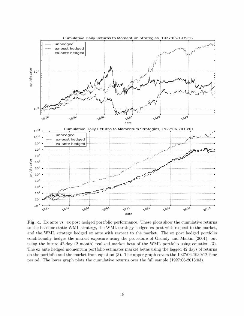
Fig. 4. Ex ante vs. ex post hedged portfolio performance. These plots show the cumulative returnsto the baseline static WML strategy, the WML strategy hedged ex post with respect to the market,and the WML strategy hedged ex ante with respect to the market. The ex post hedged portfolioconditionally hedges the market exposure using the procedure of Grundy and Martin (2001), butusing the future 42-day (2 month) realized market beta of the WML portfolio using equation (3).The ex ante hedged momentum portfolio estimates market betas using the lagged 42 days of returnson the portfolio and the market from equation (3). The upper graph covers the 1927:06-1939:12 timeperiod. The lower graph plots the cumulative returns over the full sample (1927:06-2013:03).

18

3.4. Ex ante versus ex post hedge of market risk for WML

The results of the preceding analysis suggest that calculating hedge ratios based on future

realized betas, as in Grundy and Martin (2001), is likely to produce strongly upward biased

estimates of the performance of the hedged portfolio. This is because the realized market beta

of the momentum portfolio is more negative when the realized return of the market is positive.

Thus, hedging ex post – where the hedge is based on the future realized portfolio beta – takes

more market exposure (as a hedge) when the future market return is high, leading to a strong

upward bias in the estimated performance of the hedged portfolio.

As an illustration of the magnitude of the bias, Figure 4 plots the cumulative log return to

the unhedged, ex post hedged, and an ex ante hedged WML momentum portfolio.6 The ex

post hedged portfolio takes the WML portfolio and hedges out market risk using an ex post

estimate of market beta. Following Grundy and Martin (2001), we construct the ex post

hedged portfolio based on WML’s future 42-day (2 month) realized market beta, estimated

using daily data. Again, to calculate the beta we use 10 daily lags of the market return. The

ex ante hedged portfolio estimates market betas using the lagged 42 days of returns of the

portfolio on the market, including 10 daily lags.

The first graph in Figure 4 plots the cumulative log returns to all three momentum portfolios

over the June 1927 to December 1939 period, covering a few years before, during, and after

the biggest momentum crash. The ex post hedged portfolio exhibits considerably improved

performance over the unhedged momentum portfolio as it is able to avoid the crash. However,

the ex ante hedged portfolio is not only unable to avoid or mitigate the crash, but also

underperforms the unhedged portfolio over this period. Hence, trying to hedge ex ante, as an

investor would in reality, would have made an investor worse off. The bias in using ex post

betas is substantial over this period.

The second graph in Figure 4 plots the cumulative log returns of the three momentum port-

folios over the full sample period from 1927:01-2013:03. Again, the strong bias in the ex post

hedge is clear, as the ex ante hedged portfolio performs no better than the unhedged WML

portfolio in the overall period and significantly worse than the ex post hedged portfolio.

6The calculation of cumulative returns for long-short portfolios is described in Appendix A.1.

19

Table 5Momentum Returns and Estimated Market VarianceEach column of this table presents the estimated coefficients and t-statistics for a time-seriesregression based on the following regression specification:

RWML,t = γ0 + γB · IB,t−1 + γσ2m· σ2m,t−1 + γint · IB,t−1 · σ2m,t−1 + εt,

where IB,t−1 is the bear market indicator and σ2m,t−1 is the variance of the daily returns onthe market, measured over the 126-days preceding the start of month t. The regression is estimatedusing monthly data over the period 1927:07-2013:03. The coefficients γ0 and γB are ×100 (i.e., arein percent per month).

(1) (2) (3) (4) (5)

γ0 1.955 2.428 2.500 1.973 2.129(6.6) (7.5) (7.7) (7.1) (5.8)

γB -2.626 -1.281 0.023(-3.8) (-1.6) (0.0)

γσ2m

-0.330 -0.275 -0.088(-5.1) (-3.8) (-0.8)

γint -0.397 -0.323(-5.7) (-2.2)

3.5. Market stress and momentum returns

A casual interpretation of the results presented in Section 3.2 is that, in a bear market, the

portfolio of past losers behaves like a call option on the market, and that the value of this

option is not adequately reflected in the prices of these assets. This leads to a high expected

return on the losers in bear markets, and a low expected return to the WML portfolio that

shorts these past losers. Since the value of an option on the market is increasing in the market

variance, this interpretation further suggests that the expected return of the WML portfolio

should be a decreasing function of the future variance of the market.

To examine this hypothesis, we use daily market return data to construct an ex ante estimate

of the market volatility over the coming month, and use this market variance estimate in com-

bination with the bear-market indicator, IB,t−1, to forecast future WML returns. Specifically,

we run the following regression:

RWML,t = γ0 + γB · IB + γσ2m· σ2

m,t−1 + γint · IB · σ2m,t−1 + εt, (4)

20

where IB is the bear market indicator and σ2m,t−1 is the variance of the daily returns of the

market over the 126-days prior to time t.

Table 5 reports the regression results, showing that both estimated market variance and

the bear market indicator independently forecast future momentum returns. Columns (1)

and (2) report regression results for each variable separately and column (3) reports results

using both variables simultaneously. The results are consistent with those from the previous

section: in periods of high market stress, as indicated by bear markets and high volatility,

future momentum returns are low. Finally, the last two columns of Table 5 report results for

the interaction between the bear market indicator and volatility, where momentum returns

are shown to be particularly poor during bear markets with high volatility.

3.6. Exposure to other risk factors

Our results show that time varying exposure to market risk cannot explain the low returns

of the momentum portfolio in “crash” states. However, the option-like behavior of the mo-

mentum portfolio raises the intriguing question of whether the premium associated with mo-

mentum might be related to exposure to variance risk since, in panic states, a long-short

momentum portfolio behaves like a short (written) call option on the market and since short-

ing options (i.e., selling variance) has historically earned a large premium (Christensen and

Prabhala, 1998; Carr and Wu, 2009).

To assess the dynamic exposure of the momentum strategy to variance innovations, we regress

daily WML returns on the inferred daily (excess) returns of a variance swap on the S&P 500,

which we calculate using the VIX and S&P 500 returns. Appendix A.2 provides details of

the swap return calculation. We run a time-series regression with a conditioning variable

designed to capture the time-variation in factor loadings on the market, and potentially on

other variables. The conditioning variable IBσ2 ≡ (1/vB)IB,t−1σ2m,t−1 is the interaction used

earlier but with a slight twist:

• IB is the bear market indicator defined earlier (IB = 1 if the cumulative past two-yearmarket return is negative, and is zero otherwise).

• σ2m is the variance of the market excess return over the preceding 126 days.

• (1/vB) is the inverse of the full-sample mean of σ2m over all months in which IB,t−1 = 1.

21

Table 6Regression of WML returns on variance swap returnsThis table presents the results of three daily time-series regressions of the zero-investment WMLportfolio returns on an intercept α, on the normalized ex ante forecasting variable IB,t−1σ

2m, and

on this forecasting variable interacted with the excess market return and the return on a (zero-investment) variance swap on the S&P 500. (See Appendix A.2 for details on how these swapreturns are calculated.) The sample is January 2, 1990 to March 28, 2013. T-statistics are inparentheses. The intercept (α) and the coefficient for IBσ2 are converted to annualized, percentageterms by multiplying by 252× 100.

(1) (2) (3)

α 31.48 29.93 30.29(4.7) (4.8) (4.9)

IBσ2 -58.62 -49.16 -54.83(-5.2) (-4.7) (-5.3)

rem,t 0.11 0.10(4.5) (3.1)

IBσ2 · rem,t -0.52 -0.63(-28.4) (-24.7)

rvs,t -0.02(-0.4)

IBσ2 · rvs,t -0.10(-4.7)

Normalizing the interaction term with the constant 1/vB does not affect the statistical signif-

icance of the results, but it gives the coefficients a simple interpretation. Specifically, since

∑IB,t−1=1

IBσ2 = 1,

the coefficients on IBσ2 and on variables interacted with IBσ2 can be interpreted as the weighted

average change in the corresponding coefficient during a bear market, where the weight on

each observation is proportional to the ex-ante market variance leading up to that month.

Table 6 presents the results of this analysis. In regression (1) the intercept (α) estimates

the mean return of the WML portfolio when IB,t−1 = 0 as 31.48% per year. However, the

coefficient on IBσ2 shows that the weighted-average return in “panic” periods (volatile bear

markets) is almost 59% per year lower.

Regression (2) controls for the market return and conditional market risk. Consistent with

22

our earlier results, the last coefficient in this column shows that the estimated WML beta falls

by 0.518 (t = −28.4) in panic states. However, both the mean WML return in calm periods

and the change in the WML premium in the panic periods (given, respectively, by α and the

coefficient on IBσ2), remain about the same.

In regression (3), we add the return on the variance swap and its interaction with IBσ2 .

The coefficient on rvs,t shows that outside of panic states (i.e., when IB,t−1 = 0), the WML

return does not covary significantly with the variance swap return. However, the coefficient

on IBσ2 · rvs,t shows that in panic states, WML has a strongly significant negative loading on

the variance swap return. That is, WML is effectively “short volatility” during these periods.

This is consistent with our previous results, where WML behaves like a short call option, but

only in panic periods; outside of these periods, there is no evidence of any optionality.

However, the intercept and estimated IBσ2 coefficient in regression (3) are essentially un-

changed, even after controlling for the variance swap return. The estimated WML premium

in non-panic states remains large, and the change in this premium in panic states (i.e., the

coefficient on IBσ2) is just as negative as before, indicating that although momentum returns

are related to variance risk, neither the unconditional nor conditional returns to momentum

are explained by it.

We also regress the WML momentum portfolio returns on the three Fama and French (1993)

factors consisting of the CRSP VW index return in excess of the risk-free rate, a small minus

big (SMB) stock factor, and a high BE/ME minus low BE/ME (HML) factor, all obtained

from Ken French’s website. In addition, we interact each of the factors with the panic state

variable IBσ2 . The results are reported in Appendix B, where the abnormal performance

of momentum continues to be significantly more negative in bear market states, whether we

measure abnormal performance relative to the market model or to the Fama and French (1993)

three-factor model, with little difference in the point estimates.7

7Although beyond the scope of this paper, we also examine HML and SMB as the dependent variablein similar regressions. We find that HML has opposite signed market exposure in panic states relative toWML, which isn’t surprising since value strategies buy long-term losers and sell winners, the opposite ofwhat a momentum strategy does. The correlation between WML and HML is −0.50. However, an equalcombination of HML and WML does not completely hedge the panic-state optionality as the effects on WMLare quantitatively stronger. The details are provided in Appendix B.

23

4. Dynamic weighting of the momentum portfolio

Using the insights from the previous section, we evaluate the performance of a strategy which

dynamically adjusts the weight on the WML momentum strategy using the forecasted return

and variance of the strategy. We show that the dynamic strategy generates a Sharpe ratio

more than double that of the baseline $1-long/$1-short WML strategy and is not explained by

other factors or other suggested dynamic momentum portfolios such as a constant volatility

momentum strategy (Barroso and Santa-Clara, 2012). Moreover, we employ an out-of-sample

dynamic momentum strategy that is implementable in real time and show that this portfolio

performs about as well as an in-sample version whose parameters are estimated more precisely

over the full sample period.

We begin with the design of the dynamic strategy. We show in Appendix C that, for the

objective function of maximizing the in-sample unconditional Sharpe ratio, the optimal weight

on the risky asset (WML) at time t−1 is:

w∗t−1 =

(1

2λ

)µt−1σ2t−1

(5)

where µt−1 ≡ Et−1[RWML,t] is the conditional expected return on the (zero-investment) WML

portfolio over the coming month, σ2t−1 ≡ Et−1[(R2

WML,t − µt−1)2] is the conditional variance

of the WML portfolio return over the coming month, and λ is a time-invariant scalar that

controls the unconditional risk and return of the dynamic portfolio. This optimal weighting

scheme comes from an intertemporal version of Markowitz (1952) portfolio optimization.

We then use the insights from our previous analysis to provide an estimate of µt−1, the condi-

tional mean return of WML. The results from Table 5 provide us with an instrument for the

time t conditional expected return on the WML portfolio. As a proxy for the expected return,

we use the fitted regression of the WML returns on the interaction between the bear-market

indicator IB,t−1 and the market variance over the preceding 6-months – i.e., the regression

estimated in the fourth column of Table 5.

To forecast the volatility of the WML series, we first fit a GARCH model as proposed by

Glosten, Jagannathan, and Runkle (1993, GJR) to the WML return series. The process is

defined by:

RWML,t = µ+ εt, (6)

24

where εt ∼ N (0, σ2t ) and where the evolution of σ2

t is governed by the process:

σ2t = ω + βσ2

t−1 + (α + γI(εt−1 < 0)) ε2t−1 (7)

where I(εt−1 < 0) is an indicator variable equal to one if εt−1 < 0, and zero otherwise.8 We

use maximum likelihood to estimate the parameter set (µ, ω, α, γ, β) over the full time series

(estimates of the parameters and standard errors are provided in Appendix D).

We form a linear combination of the forecast of future volatility from the fitted GJR-GARCH

process with the realized standard deviation of the 126 daily returns preceding the current

month. We show in Appendix D that both components contribute to forecasting future daily

realized WML volatility.

Our analysis in this section is also related to work by Barroso and Santa-Clara (2012), who

argue that momentum crashes can be avoided with a momentum portfolio that is scaled by

its trailing volatility. They further show that the unconditional Sharpe ratio of the constant-

volatility momentum strategy is far better than a simple $1-long/$1-short strategy.

Equation (5) shows that our results would be approximately the same as those of Barroso and

Santa-Clara (2012) if the Sharpe ratio of the momentum strategy were time-invariant, i.e.,

if the forecast mean were always proportional to the forecast volatility. Equation (5) shows

that, in this setting, the weight on WML would be inversely proportional to the forecast WML

volatility – that is the optimal dynamic strategy would be a constant volatility strategy like

the one proposed by Barroso and Santa-Clara (2012).

However, this is not the case for momentum. In fact, the return of WML is actually nega-

tively related to the forecast WML return volatility, related in part to our findings of lower

momentum returns following periods of market stress. This means that the Sharpe ratio of

the optimal dynamic portfolio varies over time, and indeed is lowest when WML’s volatility

is forecast to be high (and its mean return low). To test this hypothesis, we implement a

dynamic momentum portfolio using these insights in the next subsection, and show that the

dynamic strategy outperforms a constant volatility strategy.

To better illustrate this, Figure 5 plots the weight on the ($1-long/$1-short) WML portfolio

8Engle and Ng (1993) investigate the performance of a number of parametric models in explaining dailymarket volatility for Japan. They find that the GJR model that we use here best fits the dynamic structureof volatility for that market.

25

1929 1939 1949 1959 1969 1979 1989 1999 2009date

1

0

1

2

3

4

5

6W

eig

ht

on w

ml

Strategy Weights

wml (µ=1.00, σ=0.00)

cvol (µ=1.27, σ=0.29)

dyn (µ=1.47, σ=1.05)

Fig. 5. Dynamic strategy weights on WML

for the three strategies: the baseline WML strategy, the constant-volatility strategy (“cvol”),

and the dynamic strategy (“dyn”) with a WML weight given by equation (5). Here, we scale

the weights of both the constant volatility in the dynamic strategy to make the full sample

volatilities equal to that of the baseline WML strategy. Also, in the legend we indicate the

average weight on WML for each strategy, and the time series standard deviation of the WML

weight by strategy.

The baseline dollar long-dollar short WML strategy has, of course, a constant weight of 1.

In contrast, the constant volatility strategy WML-weight varies more, reaching a maximum

of 2.18 in November 1952, and a minimum of 0.53 in June 2009. The full dynamic strategy

weights are 3.6 times more volatile than the constant volatility weights, reaching a maximum

of 5.37 (also in November 1952), and a minimum of -0.604 in March 1938. Unlike the constant-

volatility strategy, for which the weight cannot go below zero, the dynamic strategy weight is

negative in 82 of the months in our sample – necessarily in months where the forecast-return

of the WML strategy is negative.

26

This result indicates that the dynamic strategy, at times, employs considerably more leverage

than the constant-volatility strategy. In addition, an actual implementation of the dynamic

strategy would certainly incur higher transaction costs than the other two strategies. These

factors should certainly be taken into account in assessing practical implications of the strong

performance of the strategy.

4.1. Dynamic strategy performance

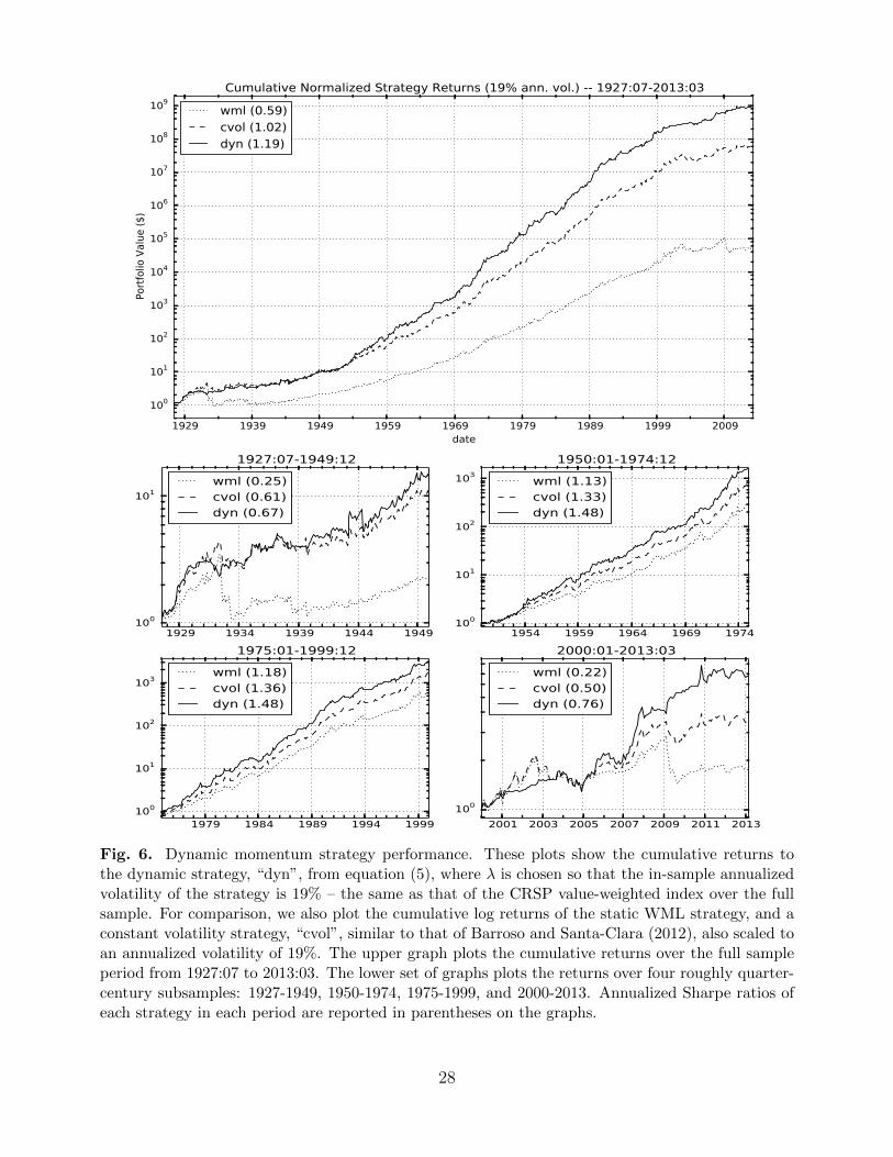
Figure 6 plots the cumulative returns to the dynamic strategy from July 1927 to March 2013,

where λ is chosen so that the in-sample annualized volatility of the strategy is 19% – the

same as that of the CRSP value-weighted index over the full sample. For comparison, we

also plot the cumulative log returns of the static WML strategy, and the constant volatility

strategy, both also scaled to 19% annual volatility. As Figure 6 shows, the dynamic portfo-

lio outperforms the constant volatility portfolio, which in turn outperforms the basic WML

portfolio. The Sharpe ratio (in parentheses on the figure) of the dynamic portfolio is nearly

twice that of the static WML portfolio and a bit higher than the constant volatility momen-

tum portfolio. In Section 4.4 we will conduct formal spanning tests among these portfolios

as well as other factors. Consistent with our previous results, part of the outperformance of

the dynamic strategy comes from its ability to mitigate momentum crashes. However, the

dynamic strategy outperforms the other momentum strategies even outside of the 1930s and

the financial crisis period, as we discuss next.

4.2. Subsample performance

As a check on the robustness of our results, we perform the same analysis over a set of

approximately quarter-century subsamples: 1927 to 1949, 1950 to 1974, 1975 to 1999, and 2000

to 2013. We use the same mean and variance forecasting equation and the same calibration

in each of the four subsamples. Figure 6 plots the cumulative log returns by subsample and

presents the strategy Sharpe ratios (in parentheses) by subsample. For these plots, returns

for each of the strategies are scaled to an annualized volatility of 19% in each subsample for

ease of comparison.

In each of the four subsamples, the ordering of performance remains the same: the dynamic

27

1929 1939 1949 1959 1969 1979 1989 1999 2009date

100

101

102

103

104

105

106

107

108

109

Port

folio

Val

ue

($)

Cumulative Normalized Strategy Returns (19% ann. vol.) -- 1927:07-2013:03

wml (0.59)cvol (1.02)dyn (1.19)

1929 1934 1939 1944 1949100

101

1927:07-1949:12

wml (0.25)cvol (0.61)dyn (0.67)

1954 1959 1964 1969 1974100

101

102

103

1950:01-1974:12

wml (1.13)cvol (1.33)dyn (1.48)

1979 1984 1989 1994 1999100

101

102

103

1975:01-1999:12

wml (1.18)cvol (1.36)dyn (1.48)

2001 2003 2005 2007 2009 2011 2013

100

2000:01-2013:03

wml (0.22)cvol (0.50)dyn (0.76)

Fig. 6. Dynamic momentum strategy performance. These plots show the cumulative returns tothe dynamic strategy, “dyn”, from equation (5), where λ is chosen so that the in-sample annualizedvolatility of the strategy is 19% – the same as that of the CRSP value-weighted index over the fullsample. For comparison, we also plot the cumulative log returns of the static WML strategy, and aconstant volatility strategy, “cvol”, similar to that of Barroso and Santa-Clara (2012), also scaled toan annualized volatility of 19%. The upper graph plots the cumulative returns over the full sampleperiod from 1927:07 to 2013:03. The lower set of graphs plots the returns over four roughly quarter-century subsamples: 1927-1949, 1950-1974, 1975-1999, and 2000-2013. Annualized Sharpe ratios ofeach strategy in each period are reported in parentheses on the graphs.

28

strategy outperforms the constant volatility strategy, which outperforms the static WML

strategy. As the subsample plots show, part of the improved performance of the constant

volatility, and especially dynamic strategy, over the static WML portfolio is the amelioration

of big crashes, but even over sub-periods devoid of those crashes, there is still improvement.

4.3. Out-of-sample performance

One important potential concern with the results presented here is that the trading strategy

relies on parameters estimated over the full sample. This is a particular concern here, as

our dynamic strategy relies on the conditional expected WML-return estimate from the fitted

regression in column (4) of Table 5.

To shed some light on whether the dynamic strategy returns could have been achieved by an

actual investor who would not have known these parameters, we construct an “out-of-sample”

strategy. We continue to use equation (5) to determine the weight on the WML portfolio, and

we continue to use the fitted-regression specification in column (4) of Table 5 for the forecast

mean, that is:

µt−1 ≡ Et−1[RWML,t] = γ0,t−1 + γint,t−1 · IB,t−1 · σ2m,t−1, (8)

only now the γ0,t−1 and γint,t−1 in our forecasting specification are the estimated regression

coefficients not over the full sample, but rather from a regression run from the start of our

sample (1927:07) up through month t−1.9 To estimate the month t WML variance we use

the 126-day WML variance estimated through the last day of month t−1.

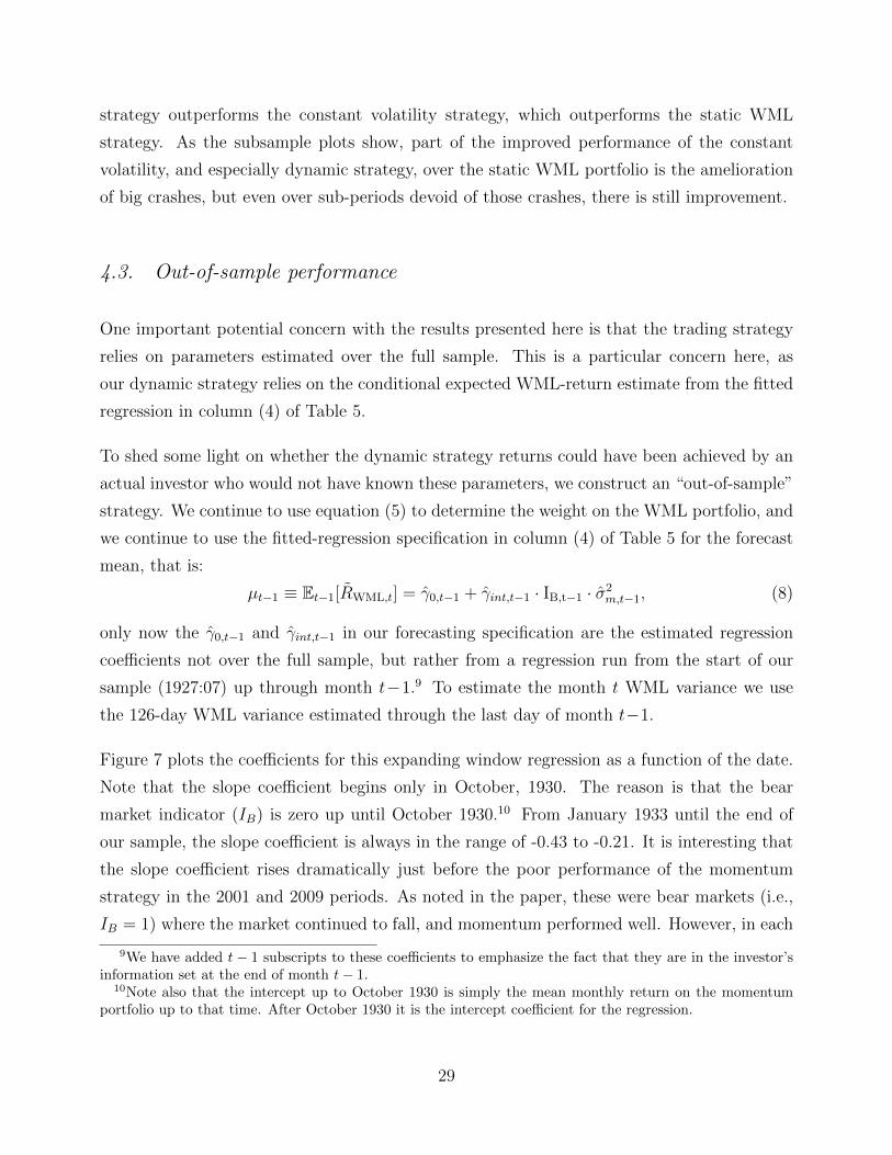
Figure 7 plots the coefficients for this expanding window regression as a function of the date.

Note that the slope coefficient begins only in October, 1930. The reason is that the bear

market indicator (IB) is zero up until October 1930.10 From January 1933 until the end of

our sample, the slope coefficient is always in the range of -0.43 to -0.21. It is interesting that

the slope coefficient rises dramatically just before the poor performance of the momentum

strategy in the 2001 and 2009 periods. As noted in the paper, these were bear markets (i.e.,

IB = 1) where the market continued to fall, and momentum performed well. However, in each

9We have added t− 1 subscripts to these coefficients to emphasize the fact that they are in the investor’sinformation set at the end of month t− 1.

10Note also that the intercept up to October 1930 is simply the mean monthly return on the momentumportfolio up to that time. After October 1930 it is the intercept coefficient for the regression.

29

1929 1939 1949 1959 1969 1979 1989 1999 2009date

1.0

0.5

0.0

0.5

1.0

1.5

coef

ficie

nts

Expanding Window Regression Coefficients

IB-sig2mintercept

Fig. 7. Mean forecast coefficients: expanding window. We use the fitted-regression specification incolumn (4) of Table 5 for the forecast mean, that is: µt−1 ≡ Et−1[RWML,t] = γ0,t−1 + γint,t−1 · IB,t−1 ·σ2m,t−1, only now the γ0,t−1 and γint,t−1 are the estimated regression coefficients not over the fullsample, but rather from a regression run from the start of our sample (1927:07) up through montht − 1 (as indicated by the t − 1 subscripts on these coefficients). To estimate the month t WMLvariance we use the 126-day WML variance estimated through the last day of month t− 1.

of these cases the forecasting variable eventually “works” in the sense that momentum does

experience very bad performance, and the slope coefficient falls. Following the fairly extreme

2009 momentum crash, the slope coefficient falls below -0.40 in August and September 2009.

4.3.1. Out-of-sample strategy performance

Table 7 presents a comparison of the performance of the various momentum strategies: the

$1 long-$1 short static WML strategy, the constant volatility strategy, and strategy scaled by

variance rather than standard deviation, the dynamic out-of-sample strategy, and the dynamic

in-sample strategy. Next to each strategy (except the first one) there are two numbers. The

first number is the Sharpe ratio of that strategy over the period from January 1934 up through

the end of our sample (March 2013). The second number is the Treynor and Black (1973)

appraisal ratio of that strategy relative to the preceding one in the list. So, for example going

from WML to the constant-volatility strategy increases the Sharpe ratio from 0.682 to 1.041.

We know that to increase the Sharpe ratio by that amount you combine the WML strategy

with an (orthogonal) strategy with a SR of√

1.0412 − 0.6822 = 0.786, which is also the value

30

Table 7Strategy performance comparisonThis table presents the annualized Sharpe-ratios of five zero-investment portfolio strategies, based onthe monthly returns of these strategies over the 1934:01-2013:03 time period. WML is the baselinemomentum strategy. cvol is the constant-volatility strategy, where the WML returns each month arescaled by the realized volatility of the daily WML returns over the preceding 126 trading days. Forthe “variance scaled” portfolio, the WML returns each month are scaled by the realized variance ofthe daily WML returns over the preceding 126 trading days. For the “dyn, out-of-sample” portfolio,the WML portfolio weights each month are multiplied each month by w∗ in equation (5), where µt−1is the out-of-sample WML mean-return forecast (equation 8), and σ2t−1 is the realized variance of thedaily WML returns over the preceding 126 trading days. The strategy labeled “dyn, in-sample” isthe dynamic strategy discussed earlier in this section. The column labeled AR gives the annualizedTreynor and Black (1973) Appraisal Ratio of the strategy in that row, relative to the strategy in thepreceding row.

Strategy SR AR†

WML 0.682cvol 1.041 0.786variance scaled 1.126 0.431dyn, out-of-sample 1.194 0.396dyn, in-sample 1.202 0.144

†AR is the annualized Treynor and Black (1973) appraisal ratio of the strategy in that row, relative to thestrategy in the preceding row.

of the Treynor-Black appraisal ratio.

Interestingly, the last two rows of this table show that going from in-sample to out-of-sample

results in only a very small decrease in performance for the dynamic strategy. Going from the

constant volatility strategy to the out-of-sample dynamic strategy continues to result in a fairly

substantial performance increase equivalent to adding on an orthogonal strategy with a Sharpe

ratio of√

1.1942 − 1.0412 = 0.585. Note that this performance increase can be decomposed

into two roughly equal parts: one part is the performance increase that comes from scaling by

variance instead of by volatility, and the second component comes from forecasting the mean,

which continues to result in a substantial performance gain (AR=0.396) even though we are

doing a full out-of-sample forecast of the mean return and variance of WML here.

31

Table 8Spanning tests of the dynamic momentum portfolioThis table presents the results of spanning tests of the dynamic (Panel A) and constant volatility(Panel B) portfolios with respect to the market (Mkt), Fama and French (1993) factors (Mkt, SMB,HML), the static WML portfolio, and each other by running daily time-series regressions of the dy-namic portfolio’s (dyn) and constant volatility (cvol) portfolio’s returns on these factors. In addition,we interact each of these factors with the market stress indicator IBσ2 to estimate conditional betaswith respect to these factors, which are labeled “conditional.” For ease of comparison the dyn andcvol portfolios are scaled to have the same annualized volatility as the static WML portfolio (23%).The reported intercepts or α’s from these regressions are converted to annualized, percentage termsby multiplying by 252× 100.

Panel A: Dependent variable = returns to dynamic (dyn) momentum portfolio(1) (2) (3) (4) (5) (6)

Model: Mkt+WML Mkt+WML FF+WML Mkt+cvol Mkt+cvol FF+cvolconditional conditional conditional conditional

α 23.74 23.23 22.04 7.27 6.92 6.10t(α) (11.99) (11.76) (11.60) (6.86) (6.44) (6.08)

Panel B: Dependent variable = returns to constant volatility (cvol) momentum portfolio(1) (2) (3) (4) (5) (6)

Model: Mkt+WML Mkt+WML FF+WML Mkt+dyn Mkt+dyn FF+dynconditional conditional conditional conditional

α 14.27 14.28 13.88 -0.72 -0.15 -0.02t(α) (11.44) (11.55) (11.28) (-0.66) (-0.13) (-0.02)

4.4. Spanning tests

A more formal test of the dynamic portfolio’s success is to conduct spanning tests with respect

to the other momentum strategies and other factors. Using daily returns, we regress the

dynamic portfolio’s returns on a host of factors that include the market and Fama and French

(1993) factors as well as the static WML and constant volatility (cvol) momentum strategies.

The annualized alphas from these regressions are reported in Table 8.

The first column of Panel A of Table 8 reports results from regressions of our dynamic mo-

mentum portfolio on the market plus the static momentum portfolio, WML. The intercept is

highly significant at 23.74% per annum (t-stat = 11.99), indicating that the dynamic port-

folio’s returns are not captured by the market or the static momentum portfolio. Since this

regression only controls for unconditional market exposure, the second column of Panel A re-

ports regression results that include interactions of our panic state indicators with the market

to capture the conditional variability in beta. The alpha is virtually unchanged and remains

32

positive and highly significant. The third column then adds the Fama and French (1993)

factors SMB and HML and their interactions with the panic state variables to account for

conditional variability in exposure to the market, size, and value factors, where the latter has

been shown, for instance, to greatly improve the performance of a momentum portfolio (e.g.,

Asness, Moskowitz, and Pedersen (2013)). This regression accounts for whether our dynamic

portfolio is merely rotating exposure to these factors.11 Again, the alpha with respect to this

conditional model is strong and significant at 22% per year, nearly identical in magnitude

to the first two columns. Hence, our dynamic momentum strategy’s abnormal performance

is not being driven by dynamic exposure to these other factors or to the static momentum

portfolio.

Columns (4) through (6) of Panel A of Table 8 repeat the regressions from columns (1) through

(3) by replacing the static WML portfolio with the constant volatility (cvol) momentum

portfolio. The alphas drop in magnitude to about 7% per year, but remain highly statistically

significant (t-stats between 6 and 7), suggesting that the dynamic momentum portfolio is not

spanned by the constant volatility portfolio.

Panel B of Table 8 flips the analysis around and examines whether the constant volatility

portfolio is spanned by the static WML portfolio or the dynamic portfolio. The first three

columns of Panel B indicate that the constant volatility portfolio is not spanned by the static

WML portfolio or the Fama and French (1993) factors, generating alphas of about 14% per

annum with highly significant t-statistics. These results are consistent with Barroso and Santa-

Clara (2012). However, the alphas of the constant volatility portfolio are slightly smaller in

magnitude than those from the dynamic strategy, consistent with the Sharpe ratio comparisons

from Figure 6. (Since we scale both the dynamic and constant volatility portfolios to have the

same variance, these alphas are comparable and give the same rankings as information ratios

would.)

Columns (4) through (6) of Panel B report results from regressing the constant volatility

portfolio’s returns on the dynamic portfolio’s returns. Here, the alphas are all zero, both eco-

nomically and statistically, suggesting that the dynamic portfolio spans the constant volatility

portfolio. According to Appendix C, this should be the case in theory, thus implying that

11 Since the optimal dynamic portfolio solved in Appendix C is not conditional on other factors, to form thisportfolio in the presence of other factors we first regress the static momentum portfolio on the other factorsusing daily returns and then use the residuals to form our dynamic strategy by forecasting the conditionalmean and variance of those residuals to form the dynamic weights.

33

we obtain decent ex ante forecasts of the conditional mean and variance of the static WML

portfolio to form a dynamic strategy that reliably captures and improves upon the returns to

a constant volatility and static momentum portfolio.

5. International equities and other asset classes

Although first documented in individual equities in the US, subsequent research has demon-

strated the existence of strong momentum effects among common stocks in other investment

regions and in other asset classes (see Asness, Moskowitz, and Pedersen (2013) for a summary).

We investigate whether the same momentum crash patterns we observe in US equities are

also present in these other asset markets, and whether our dynamic momentum portfolio

helps ameliorate these crashes and improves momentum performance in other markets..

5.1. Data

The data come from Asness, Moskowitz, and Pedersen (2013) and for equities cover the U.S.,

U.K., Japan, and Continental Europe. Details on data description and sources can be found

in Asness, Moskowitz, and Pedersen (2013). The US and UK data begin in January 1972

and Europe and Japan in February 1974, extending to May 2013.12 We also examine a global

equity momentum strategy GE, which weights each region’s equity momentum strategy by

the ex post volatility of the portfolio over the full sample, following Asness, Moskowitz, and

Pedersen (2013).

The non-equity data also come from Asness, Moskowitz, and Pedersen (2013), which contain

equity country index futures across 18 developed equity markets beginning in January 1978, 10

currencies across developed markets starting in January 1979, 10 country government bonds

beginning January 1982, and 27 different commodity futures beginning in January 1972. All

series end in May 2013.

12These data extend beyond the original sample period used in Asness, Moskowitz, and Pedersen (2013),since the data are updated monthly following the same procedure for portfolio construction in Asness,Moskowitz, and Pedersen (2013). The data are available from Toby Moskowitz’s website:(http://faculty.chicagobooth.edu/tobias.moskowitz/research/data.html).

34

In addition, we examine two composite portfolios: GA is a global momentum strategy across

the non-equity asset classes, which weights each asset class momentum strategy portfolio by

the ex post volatility of that portfolio. GAll is a global momentum strategy across all of the

equity and non-equity asset classes, which weights the GE and GA portfolios by their ex post

return volatilities over the full sample.

The definition of the market index is different for each market and asset class: it is the MSCI

local index for the US, UK, Europe, and Japan, the MSCI World index for country index

futures, an equal-weighted average of all country bonds for bond markets, an equal-weighted

average of all currencies for currency markets, and the Goldman Sachs Commodity Index

(GSCI) for commodities.

5.2. Cross sectional equity momentum outside the US

The portfolio formation procedure here is similar to that used earlier in the paper, except

instead of taking the top and bottom decile portfolios, we use the Asness, Moskowitz, and

Pedersen (2013) P3−P1 momentum portfolios, which is long the top third and short the

bottom third of securities ranked on returns from month t − 12 to t − 2. Both the long and

the short side of the portfolio are value weighted. As documented in Asness, Moskowitz,

and Pedersen (2013), over this time period there are strong momentum effects in each of the

regions except Japan.

Panels A through D of Table 9 present the results of the regressions run in Section 2, but here

for the other stock market universes. Panel A shows the estimated coefficients and t-statistics

from the regression specification in equation (2). Consistent with the results presented earlier,

the market betas of the momentum strategy are dramatically lower in bear markets across

the other stock markets as well. The strategies implemented using European and Japanese

stocks have market betas that are approximately 0.5 lower during bear markets (with t-stats

of about -7). The UK momentum strategy beta falls by 0.2. The drop in this period for the

US momentum strategy is 0.58 – comparable to what we observe for the WML portfolio over

the longer 1927 to 2013 period. Globally, averaging across the US, UK, Europe, and Japan,

the market betas of the momentum strategy are markedly lower in bear markets.

The abnormal returns of the momentum strategies are significantly positive in bull markets

35

for all regions except Japan. Consistent with our analysis in Section 2, the return is lower in

bear markets in each region, though using only the bear market indicator as a proxy for panic

periods none of the differences are statistically significant over these shorter sample periods.

Panel B investigates the optionality in the momentum strategy in bear markets using the

regression specification in equation (3). Consistent with the longer period US results, there

is statistically significant optionality in bear markets in the European, UK, and Japan stock

markets, and globally across all markets. Interestingly, for this subsample and methodology,

the optionality is of the right sign, but is not statistically significant for the US market. The

negative beta of long-short momentum strategies is particularly acute when the contempora-

neous market return is positive. That is, momentum strategies in all regions across the world

exhibit conditional betas and payoffs similar to writing call options on the local market index.

In Panel C, we add as a conditioning variable the realized daily market return variance,

annualized, over the preceding 126 trading days (6 months):13

RP3−P1t = [α0 + αBIB,t−1 + αV σ

2m,t−1] + [β0 + βBIB,t−1 + βV σ

2m,t−1]R

em,t + εt. (9)

Two interesting results emerge. First, higher ex ante market variance is generally associated

with more negative momentum strategy betas. Second, higher market variance is also asso-

ciated with strongly lower future abnormal returns to momentum, net of the market return.

This last relation is statistically significant in all markets, and again is consistent with our

earlier results for the US market over the longer period.

In Panel D we again use the IBσ2 ≡ (1/vB)IB,t−1 · σ2m measure introduced in Section 3.6,

designed to capture “panic” periods when the market has fallen and volatility is high. In

addition, in these regressions we instrument for time variation in market beta using IB,t−1,

σ2m,t−1, and IBσ2 . Specifically, we run the regression

RP3−P1t = [α0 + αBIBσ2 ] + [βBIB,t−1 + βVσ

2m,t−1 + βBVIBσ2 ]Re

m,t + εt. (10)

The results in Panel D of Table 9 are consistent with our earlier results for the US over

the longer period. In particular, the coefficient on the interaction term IBσ2 is negative,

13This is the same market variance measure used earlier. However, for the EU, JP, and UK regions we havedaily MSCI market return data only for the time period from January 1990 on. Therefore, over the periodfrom 1972:01-1990:06 in the UK, and 1974:02-1990:06 in EU and JP, we use the realized monthly varianceover the preceding 6 months, again annualized.

36

economically large, and statistically significant in all markets, and for the global strategy.

In summary, the results in Table 9 suggest that momentum strategies in these different equity

markets are also short volatility, and have significantly lower abnormal returns in panic periods

characterized by poor lagged market returns and high market volatility.

One other point of interest is that, in Panels C and D of Table 9, the α for the Japan

momentum strategy is considerably larger, and in Panel C is in fact significant at a 5% level.

We will explore the implications of this finding further in Section 5.4, where we apply a

dynamic Japanese momentum strategy which takes into account the forecastability of both

the expected return and volatilty.

5.3. Cross-sectional momentum in other asset classes

Evidence of the option-like payoffs of momentum strategies in bear markets outside of US

equities, and indeed in every other equity market we examined, gives credence to this feature

of momentum being a robust phenomenon and not likely due to chance. For further robustness,

we also examine momentum strategies in the non-equity asset classes. In addition to providing

another out of sample test for the option-like payoffs of momentum strategies in bear markets,

finding the same option-like asymmetry in these asset classes would also present a challenge

to the Merton (1974) explanation.

Table 10 presents the results of time series regressions for the non-equity asset-class momen-

tum strategies similar to those in Table 9 for international equities. First, the set of IB,t−1·Rem

coefficients and t-statistics in the last row of Panel A show that, in all asset classes, the mo-

mentum portfolio’s market beta is significantly more negative in bear markets. The intuition

that – following a bear market, the loser side of the momentum portfolio will have a high

market beta – remains valid in the non-equity asset classes as well. The IB,t−1 coefficients in

the second row of Panel A also provide evidence weakly consistent with the earlier finding that

market-adjusted momentum returns are lower following bear markets. The point estimates

are all negative, except for bonds, but only in the currency market is the coefficient significant.

Panel B assesses whether the optionality present in cross-sectional equity momentum strategies

is also present in other asset classes. The IB,t−1IU,tRem,t coefficient is negative for each of the

four asset classes, and the two composite portfolios, but is statistically significant at a 5%

37

Table 9Time series regressions for international equity marketsThe table reports the estimated coefficients and t-statistics from regressions of the monthly returnsto a zero-investment equity momentum strategy in each region on the indicated set of independentvariables. The estimated regression intercept (α), and the coefficients on IB and IBσ2 are all mul-tiplied by 12×100 to put them in annualized, percentage terms. GE is a global equity momentumstrategy that is a volatility-weighted portfolio of the four equity markets.

EU JP UK US GEstart 1974:02 1974:02 1972:01 1972:01 1972:01end 2013:05 2013:05 2013:05 2013:05 2013:05

Panel Aα 8.935 1.887 7.409 5.181 5.826

(3.5) (0.5) (2.7) (1.9) (3.6)IB -3.549 -0.837 -6.827 -2.921 -4.920

(-0.7) (-0.1) (-1.1) (-0.5) (-1.2)Rem 0.071 0.246 0.015 0.150 0.023

(1.6) (4.8) (0.4) (2.7) (0.7)IBR

em -0.508 -0.527 -0.197 -0.584 -0.275

(-7.1) (-7.0) (-3.1) (-6.2) (-4.6)Panel B

α 8.935 1.887 7.409 5.181 5.826(3.6) (0.5) (2.7) (1.9) (3.6)

IB 9.418 11.104 4.249 -0.266 5.019(1.2) (1.3) (0.5) (-0.0) (0.8)

Rem 0.071 0.246 0.015 0.150 0.023(1.7) (4.8) (0.4) (2.7) (0.7)

IBRem -0.302 -0.318 0.004 -0.540 -0.098

(-2.7) (-2.5) (0.0) (-3.3) (-1.0)IBIUR

em -0.418 -0.367 -0.306 -0.086 -0.342

(-2.4) (-2.0) (-2.2) (-0.3) (-2.2)Panel C

α 12.237 12.385 10.856 10.331 8.345(4.1) (2.5) (3.6) (3.4) (4.8)

IB 1.445 4.554 0.213 6.018 2.254(0.3) (0.7) (0.0) (0.9) (0.5)

σ2m -0.113 -0.221 -0.078 -0.204 -0.252

(-2.0) (-2.9) (-2.6) (-3.3) (-3.7)Rem 0.115 0.280 0.020 0.215 0.041

(2.5) (4.2) (0.5) (3.6) (1.2)IBR

em -0.391 -0.512 -0.182 -0.485 -0.206

(-4.8) (-6.5) (-2.5) (-4.8) (-3.2)σ2mR

em -1.755 -0.734 -0.040 -2.361 -1.959

(-2.6) (-0.7) (-0.2) (-2.5) (-2.2)Panel D

α 10.286 5.333 8.627 7.084 6.720(4.4) (1.6) (3.4) (2.8) (4.5)

IBσ2 -6.509 -9.910 -11.408 -11.055 -8.704(-2.0) (-2.2) (-3.2) (-2.6) (-3.6)

IBRem -0.306 -0.180 -0.176 -0.245 -0.177

(-3.7) (-1.8) (-2.6) (-2.4) (-2.8)σ2mR

em -0.295 3.685 -0.600 1.839 -2.798

(-0.2) (3.8) (-0.8) (1.2) (-1.2)IBσ2Rem -0.056 -0.307 0.073 -0.261 0.036

(-0.7) (-3.2) (0.8) (-2.4) (0.5)

38

Table 10Time series regressions for other asset classesThe table reports the estimated coefficients and t-statistics from regressions of the monthly returns to zero-

investment momentum strategies in each asset class on the indicated set of independent variables. GA and

GAll are the global strategies across all non-equity asset classes and across all asset classes including equities,

where each asset class and equity market is weighted by the inverse of their full sample volatility. The estimated

intercept, and the coefficients on IB,t−1 and IBσ2 are all multiplied by 12×100 to put them in annualized,

percentage terms.FI CM FX EQ GA GAll

start 1983:02 1973:02 1980:02 1979:02 1973:02 1973:02end 2013:05 2013:05 2013:05 2013:05 2013:05 2013:05

Panel Aα 0.006 16.302 4.745 8.575 4.653 4.639

(0.0) (3.7) (2.2) (3.8) (4.6) (5.0)IB 0.798 -10.470 -8.221 -0.575 -2.426 -3.294

(0.3) (-1.4) (-2.5) (-0.1) (-1.1) (-1.3)Rem 0.186 0.308 0.382 0.272 0.162 0.082

(3.1) (4.1) (4.4) (6.0) (2.7) (1.9)IBR

em -0.362 -0.730 -1.092 -0.620 -0.485 -0.366

(-2.7) (-4.5) (-8.6) (-8.5) (-3.9) (-4.4)Panel B

α 0.006 16.302 4.745 8.575 4.653 4.639(0.0) (3.8) (2.2) (3.8) (4.6) (5.1)

IB 1.994 7.014 -4.096 6.248 1.142 3.746(0.6) (0.7) (-0.9) (1.1) (0.4) (1.1)

Rem 0.186 0.308 0.382 0.272 0.162 0.082(3.1) (4.1) (4.4) (6.0) (2.7) (1.9)

IBRem -0.278 -0.205 -0.911 -0.485 -0.222 -0.106

(-1.4) (-0.8) (-5.0) (-4.6) (-1.2) (-0.9)IBIUR

em -0.197 -1.102 -0.405 -0.312 -0.563 -0.605

(-0.6) (-2.5) (-1.4) (-1.7) (-1.8) (-2.9)Panel C

α -0.297 20.050 7.527 9.277 5.835 5.963(-0.2) (3.5) (2.4) (3.8) (4.9) (5.9)

IB 1.057 -9.022 -7.475 0.634 -0.759 0.554(0.4) (-1.2) (-2.2) (0.2) (-0.3) (0.2)

σ2m 0.136 -0.211 -0.503 -0.047 -0.756 -0.585

(0.2) (-1.1) (-1.2) (-0.7) (-1.8) (-3.0)Rem 0.278 0.522 0.429 0.299 0.201 0.104

(2.1) (4.3) (4.0) (6.3) (3.0) (2.3)IBR

em -0.385 -0.712 -1.045 -0.549 -0.374 -0.267

(-2.8) (-4.4) (-8.0) (-6.6) (-2.7) (-2.8)σ2mR

em -55.971 -8.820 -9.702 -2.001 -23.842 -8.605

(-0.8) (-2.2) (-0.8) (-1.7) (-1.2) (-1.5)Panel D

α 0.218 13.803 3.419 9.240 4.766 4.853(0.2) (3.7) (1.8) (4.7) (5.1) (5.6)

IBσ2 0.026 -4.808 -4.655 -2.683 -2.308 -4.056(0.0) (-1.2) (-2.1) (-1.2) (-1.8) (-2.8)

Rem 0.263 0.772 0.672 0.384 0.238 0.128(1.9) (5.0) (3.0) (5.9) (2.0) (2.0)

IBRem -0.281 -1.207 -1.293 -0.669 -0.424 -0.303

(-0.8) (-4.8) (-5.0) (-6.4) (-2.3) (-2.7)σ2mR

em -46.141 -18.887 -60.175 -8.332 -49.075 -22.030

(-0.6) (-3.4) (-1.4) (-2.4) (-0.7) (-1.0)IBσ2Rem -0.105 0.344 0.268 0.222 0.074 0.095

(-0.3) (2.5) (1.3) (1.9) (0.4) (0.6)

39

level only for commodities. This result is intriguing. While a model such as Merton (1974)

argues that equities should exhibit option-like features, it is not clear that such a model would

easily explain the optionality present in commodity futures, and weakly in currency markets.

Panel C of Table 10 estimates equation (9) for the other-asset-class momentum strategies.

Here the signs of the relation between lagged volatility and momentum strategy returns are

again negative in the commodity (CM), currency (FX), and equity (EQ) futures asset classes.

Panel D again uses the interactive variable IBσ2 as an instrument for volatile bear markets.

As in Table 9, we control for variation in market beta associated with IB,t−1, σ2m, and the

interaction term itself. In all asset classes except FI, the coefficient on this interaction term

is negative, consistent with our previous findings in US and international equity markets.

However, except for FX and the GAll portfolio, the coefficient is not significant at a 5% level.

These findings are largely consistent with the results for US equities and for other equity

markets. In addition to providing more robustness, these findings also make it more difficult

to reconcile under a Merton (1974)-style theory, which is better suited for equity returns.

5.4. Dynamic strategies in other markets and asset classes

Given the robustness of the option-like features to momentum in other equity markets and

other asset classes, we examine the efficacy of the dynamic momentum strategies – constructed

as in Section 4 – to examine whether the dynamic strategy continues to perform well when

implemented in these other asset markets.

We form the dynamic momentum strategy as before using the ex-ante expected return and

volatility of the WML portfolio in each market using the instruments from the previous anal-

ysis – the interaction of the ex-ante bear market indicator for that asset class, IB,t−1, and the

asset-class market volatility over the preceding 6-months – to forecast the conditional expected

return and volatility. Precise specifications of the forecasting model and the GARCH model

parameters for each asset class are given in Appendix D.

Panel A of Table 11 reports the Sharpe ratio and skewness (in parentheses) of the simple $1

long-$1 short WML momentum strategy in each market and asset class, as well as a constant

volatility momentum strategy and the dynamic momentum strategy as described above. In

addition, we report global combinations of the equity momentum strategies across all markets

40

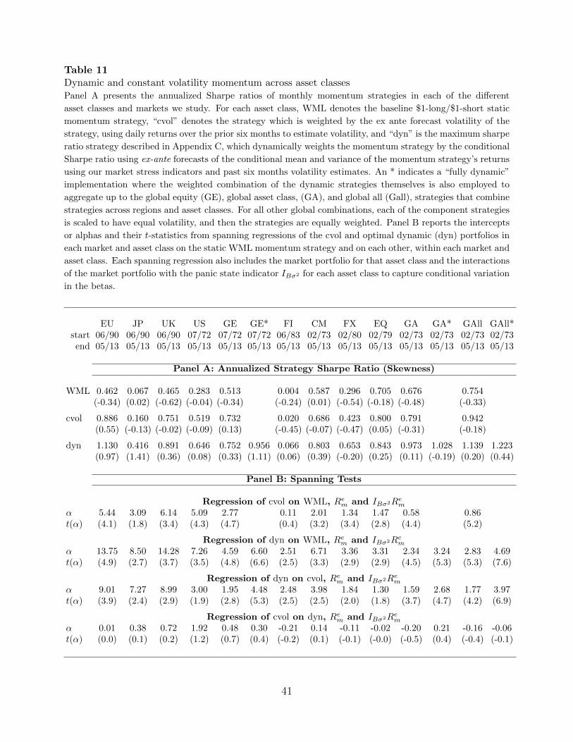
Table 11Dynamic and constant volatility momentum across asset classesPanel A presents the annualized Sharpe ratios of monthly momentum strategies in each of the different

asset classes and markets we study. For each asset class, WML denotes the baseline $1-long/$1-short static

momentum strategy, “cvol” denotes the strategy which is weighted by the ex ante forecast volatility of the

strategy, using daily returns over the prior six months to estimate volatility, and “dyn” is the maximum sharpe

ratio strategy described in Appendix C, which dynamically weights the momentum strategy by the conditional

Sharpe ratio using ex-ante forecasts of the conditional mean and variance of the momentum strategy’s returns

using our market stress indicators and past six months volatility estimates. An * indicates a “fully dynamic”

implementation where the weighted combination of the dynamic strategies themselves is also employed to

aggregate up to the global equity (GE), global asset class, (GA), and global all (Gall), strategies that combine

strategies across regions and asset classes. For all other global combinations, each of the component strategies

is scaled to have equal volatility, and then the strategies are equally weighted. Panel B reports the intercepts

or alphas and their t-statistics from spanning regressions of the cvol and optimal dynamic (dyn) portfolios in

each market and asset class on the static WML momentum strategy and on each other, within each market and

asset class. Each spanning regression also includes the market portfolio for that asset class and the interactions

of the market portfolio with the panic state indicator IBσ2 for each asset class to capture conditional variation

in the betas.

EU JP UK US GE GE* FI CM FX EQ GA GA* GAll GAll*start 06/90 06/90 06/90 07/72 07/72 07/72 06/83 02/73 02/80 02/79 02/73 02/73 02/73 02/73end 05/13 05/13 05/13 05/13 05/13 05/13 05/13 05/13 05/13 05/13 05/13 05/13 05/13 05/13

Panel A: Annualized Strategy Sharpe Ratio (Skewness)

WML 0.462 0.067 0.465 0.283 0.513 0.004 0.587 0.296 0.705 0.676 0.754(-0.34) (0.02) (-0.62) (-0.04) (-0.34) (-0.24) (0.01) (-0.54) (-0.18) (-0.48) (-0.33)

cvol 0.886 0.160 0.751 0.519 0.732 0.020 0.686 0.423 0.800 0.791 0.942(0.55) (-0.13) (-0.02) (-0.09) (0.13) (-0.45) (-0.07) (-0.47) (0.05) (-0.31) (-0.18)

dyn 1.130 0.416 0.891 0.646 0.752 0.956 0.066 0.803 0.653 0.843 0.973 1.028 1.139 1.223(0.97) (1.41) (0.36) (0.08) (0.33) (1.11) (0.06) (0.39) (-0.20) (0.25) (0.11) (-0.19) (0.20) (0.44)

Panel B: Spanning Tests

Regression of cvol on WML, Rem and IBσ2Remα 5.44 3.09 6.14 5.09 2.77 0.11 2.01 1.34 1.47 0.58 0.86t(α) (4.1) (1.8) (3.4) (4.3) (4.7) (0.4) (3.2) (3.4) (2.8) (4.4) (5.2)

Regression of dyn on WML, Rem and IBσ2Remα 13.75 8.50 14.28 7.26 4.59 6.60 2.51 6.71 3.36 3.31 2.34 3.24 2.83 4.69t(α) (4.9) (2.7) (3.7) (3.5) (4.8) (6.6) (2.5) (3.3) (2.9) (2.9) (4.5) (5.3) (5.3) (7.6)

Regression of dyn on cvol, Rem and IBσ2Remα 9.01 7.27 8.99 3.00 1.95 4.48 2.48 3.98 1.84 1.30 1.59 2.68 1.77 3.97t(α) (3.9) (2.4) (2.9) (1.9) (2.8) (5.3) (2.5) (2.5) (2.0) (1.8) (3.7) (4.7) (4.2) (6.9)

Regression of cvol on dyn, Rem and IBσ2Remα 0.01 0.38 0.72 1.92 0.48 0.30 -0.21 0.14 -0.11 -0.02 -0.20 0.21 -0.16 -0.06t(α) (0.0) (0.1) (0.2) (1.2) (0.7) (0.4) (-0.2) (0.1) (-0.1) (-0.0) (-0.5) (0.4) (-0.4) (-0.1)

41

(GE), the non-equity asset classes (GA), and a combination of all equity markets and non-

equity asset classes (GAll).

As Panel A of Table 11 shows, there is a marked improvement in Sharpe ratio going from the

static WML momentum strategy to a constant volatility momentum strategy to our dynamic

momentum strategy in every single market and asset class we study except fixed income. In

most cases, our dynamic strategy doubles the Sharpe ratio over the traditional static momen-

tum portfolio. Furthermore, our dynamic momentum strategy resurrects positive returns in

markets where the typical momentum portfolio has failed to produce positive profits, such as

Japan. In Japan, the static, classic momentum portfolio delivers a 0.07 Sharpe ratio, but our

dynamic momentum portfolio in Japan produces a 0.42 Sharpe ratio. (Alas, even the dynamic

strategy does not deliver a significant Sharpe ratio for fixed income.)

The skewness numbers (in parentheses) are also interesting, as the predominantly negative

skewness of the static momentum strategies across all markets is apparent, but the dynamic

momentum strategies deliver mostly positive skewness – consistent with amelioration of the

“crashes” we see in plots of the returns to these strategies.

We also report results for a “fully dynamic” portfolio that is a weighted combination of the

individual asset class or market dynamic strategies, where the weighs are based on the ex ante

conditional volatility of each component strategy. That is, each of the component strategies is

scaled to have equal volatility (ex ante), and then the strategies are equally weighted. In this

way, we are also using cross-sectional information on the strength of the dynamic signal of each

component strategy to build a fully dynamic combination portfolio across all asset classes. We

denote these fully dynamic strategies with a * in Table 11. As the table indicates, there is

additional Sharpe ratio improvement from this additional twist on our dynamic momentum

strategies, providing another robustness test on the use of conditional mean and variance

forecastability in enhancing the returns to momentum strategies.

Panel B of Table 11 reports results from spanning tests of the static WML portfolio, the

constant volatility strategy, and the dynamic strategy within each market and asset class.

These daily return regressions also include interactions of the excess market return and the

excess market return (for that asset class) interacted with the asset-class specific panic state

indicator IBσ2 to capture conditional variation in the betas.14 The first row reports alphas

14As with our spanning tests in Section 4, the dynamic strategy used in Panel B is based on ex ante forecastsof the mean and variance of the residual from a regression of the WML strategy on the excess market return

42

(and their t-statistics) of the constant volatility strategy on WML in each market and asset

class, as well as globally across equity markets (GE), asset classes (GA), and all markets

and asset classes (GAll). Consistent with the results of Barroso and Santa-Clara (2012)

for US equities, the constant volatility strategy delivers positive alpha relative to the static

momentum strategy in every single market and asset class that is highly significant (except

Japan and fixed income, where momentum does not yield statistically significant positive

returns to begin with).

The second row reports alphas of the dynamic momentum strategy with respect to WML.

Here too, the alphas are all positive and statistically significant, and in every single market

and asset class are larger than the constant volatility momentum alphas. Since both the

dynamic and constant volatility strategies are scaled to the same volatility, this suggests that

the dynamic momentum portfolio offers improved mean-variance efficiency over the constant

volatility portfolio, which it should according to theory.

To test this notion more formally, the last two sets of rows of Panel B of Table 11 report the

alphas from regressions of the dynamic strategy returns on the constant volatility strategy

returns, and vice-versa. The results are consistent with our previous findings: in virtually every

market and asset class the dynamic momentum portfolio delivers positive and statistically

significant alpha relative to the constant volatility strategy, suggesting that the constant

volatility strategy does not span the dynamic strategy in any market or asset class. Conversely,

in every market and asset class the constant volatility strategy fails to produce a significant

alpha with respect to the dynamic strategy, suggesting that the dynamic momentum strategy

spans the constant volatility strategy in every market and asset class. These results, shown out

of sample in eight other markets and asset classes, make a compelling case for the robustness

of the dynamic momentum portfolio based on the optionality insights of momentum strategies

in every market.

Overall, the consistent evidence of the optionality of momentum strategies, conditional betas

and return premia, and the significant improvement from our dynamic weighting scheme across

many different markets and vastly different asset classes, provides a wealth of out- of-sample

evidence. Momentum crashes and their forecastability by bear market and ex ante volatility

measures are a reliable and robust feature of momentum strategies that may provide clues as

Rem and the interacted market return IBσ2Rem, using the panic state indicator and lagged residual variancesas forecasting variables. See footnote 11.

43

to the underlying source of this return factor.15

6. Conclusions

In “normal” environments we see consistent price momentum that is both statistically and

economically strong and manifests itself across numerous equity markets and a wide range of

diverse asset classes.

However, in “panic” states, following multi-year market drawdowns and in periods of high

market volatility, the prices of past losers embody a high premium. When poor market

conditions ameliorate and the market starts to rebound, the losers experience strong gains,

resulting in a “momentum crash” as momentum strategies short these assets. We find that, in

bear market states, and in particular when market volatility is high, the down-market betas

of the past-losers are low, but the up-market betas are very large. This optionality does not

appear to generally be reflected in the prices of the past losers. Consequently, the expected

returns of the past losers are very high, and the momentum effect is reversed during these

times. This feature does not apply equally to winners during good times, however, resulting

in an asymmetry in the winner and loser exposure to market returns during extreme times.

These results are shown to be robust: we obtain consistent results in eight different markets

and asset classes, as well as in multiple time periods. Moreover, these crash periods are

predictable: we use bear market indicators and ex ante volatility estimates to forecast the

conditional mean and variance of momentum strategies. Armed with these estimates, we

create a simple dynamically-weighted version of the momentum portfolio that approximately

doubles the Sharpe ratio of the static momentum strategy and is not spanned by constant

volatility momentum strategies or other factors – doing so consistently in every market, asset

class, and time period we study.

What can explain these findings? We examine a variety of explanations ranging from compen-

sation for crash risk to volatility risk, to other factor risks such as the Fama and French (1993)

factors, but find that none of these explanations can account fully for our findings. For equity

15Although beyond the scope of this paper, it would be interesting to see if other momentum-type strategies,such as earnings momentum in equities (Chan, Jegadeesh, and Lakonishok, 1996), or time-series momentumin futures contracts (Moskowitz, Ooi, and Pedersen, 2012), or cross-momentum effects (Cohen and Frazzini,2008) exhibit similar features.

44

momentum, a Merton (1974) story for the option-like payoffs of equities may make sense, but

the existence of the same phenomena and option-like features for momentum strategies in fu-

tures, bonds, currencies, and commodities, makes this story more challenging. Alternatively,

these effects may be loosely consistent with several behavioral findings, where in extreme

situations individuals tend to be fearful and appear to focus on losses, largely ignoring prob-

abilities.16 Whether this behavioral phenomenon is fully consistent with the empirical results

documented here is a subject for further research and would indicate that the behavior of

market participants in each of these markets and asset classes is affected similarly, despite

the fact that the average and marginal investor in these various markets are likely to be quite

different along many other dimensions.

16See Sunstein and Zeckhauser (2008), Loewenstein, Weber, Hsee, and Welch (2001), and Loewenstein(2000).

45

Appendices

Appendix A. Detailed description of calculations

A.1. Cumulative return calculations

The cumulative return, on an (implementable) strategy is an investment at time 0, whichis fully reinvested at each point – i.e., where no cash is put in or taken out. That is, thecumulative arithmetic returns between times t and T is denoted R(t, T ).

R(t, T ) =T∏

s=t+1

(1 +Rs)− 1,

where Rs denotes the arithmetic return in the period ending at time t, and rs = log(1 + Rs)denotes the log-return over period s,

r(t, T ) =T∑

s=t+1

rs.

For long-short portfolios, the cumulative return is:

R(t, T ) =T∏

s=t+1

(1 +RL,s −RS,s +Rf,t)− 1,

where the terms RL,s, RS,s, and Rf,s are, respectively, the return on the long side of theportfolio, the short side of the portfolio, and the risk-free rate. Thus, the strategy reflects thecumulative return, with an initial investment of Vt, which is managed in the following way:

1. Using the $V0 as margin, you purchase $V0 of the long side of the portfolio, and short$V0 worth of the short side of the portfolio. Note that this is consistent with Reg-Trequirements. Over each period s, the margin posted earns interest at rate Rf,s.

2. At then end of each period, the value of the investments on the long and the short side ofthe portfolio are adjusted to reflect gains to both the long and short side of the portfolio.So, for example, at the end of the first period, the investments in both the long andshort side of the portfolio are adjusted to set their value equal to the total value of theportfolio to Vt+1 = Vt · (1 +RL −RS +Rf ).

This methodology assumes that there are no margin calls, etc., except at the end of eachmonth. These calculated returns do not incorporate transaction costs.

46

A.2. Calculation of variance swap returns

We calculate the returns to a daily variance swap on the S&P 500 using daily observationson the SPX and the VIX, and daily levels of the one-month Treasury bill rate. The historicaldaily observations on the SPX and the VIX, beginning on January 2, 1990, are taken from theCBOE’s VIX website.17 The daily one-month interest rate series is taken from Ken French’sdata library.

The VIX is calculated using a panel of S&P 500 index options with a wide range of strikeprices and with two maturity dates – generally the two closest-to-maturity contracts, weightedin such a way so as to most closely approximate the swap rate for a variance swap with aconstant maturity of 30 calendar days.18 The calculation method used by the CBOE makesthe VIX equivalent to the swap rate for a variance swap on the S&P 500 over the coming30 calendar days. However, the methodology used by the CBOE is to: (1) annualize thisvariance; (2) take the square-root of the variance (to convert to volatility), multiply by 100to convert to percentage terms.

Given the VIX construction methodology, we can calculate the daily return on a varianceswap, from day t−1 to day t, as:

Rvs,t = Dt

[1

21

(252

[100·log

(StSt−1

)]2−VIX2

t−1

)+

20

21

(VIX2

t−VIX2t−1)].

Here Dt is the 20-trading day discount factor. This is calculated as Dt = (1 + r1m,t)20/252,

where r1m,t is the annualized one-month treasury bill yield as of day t, from Ken French’swebsite. VIXt is the level of the VIX as quoted at the end of day t and St is the level of theS&P 500, adjusted for all corporate actions, at the end of day t. Note that the factors of 252and 100 in the equation are because the VIX is quoted in annualized, percentage terms.

This equation is given a flat forward variance curve. That is, we are implicitly making theassumption that the swap rate on 20 trading-day and 21 trading-day variance swap rates onday t are identical (and equal to VIX2

t ). For the market, this approximation should be fairlyaccurate.

Appendix B. Exposure to size and value factors

We regress the WML momentum portfolio returns on the three Fama and French (1993)factors consisting of the CRSP VW index return in excess of the risk-free rate, a small minusbig (SMB) stock factor, and a high BE/ME minus low BE/ME (HML) factor, all obtainedfrom Ken French’s website. In addition, we interact each of the factors with the panic state

17The daily data for the new VIX are available at http://www.cboe.com/micro/VIX/historical.aspx.18See Chicago Board Options Exchange (2003) for a full description of the VIX calculation.

47

Table 12Conditional estimation of WML, HML, and SMB premiaThis table presents the results of monthly time-series regressions. The dependent variable is indicatedat the head of each column, and is either: (1) WML; (2) the HML–devil portfolio proposed by Asnessand Frazzini (2011); the SMB portfolio return of Fama and French (1993); or (4) a portfolio which is50% WML and 50% HML-devil. The independent variables are: intercept α, the normalized ex anteforecasting variable IBσ2 ≡ (1/vB)IB,t−1 · σ2m, and this forecasting variable interacted with the excessmarket return and the Fama and French (1993) HML and SMB returns. The sample is January1927 through March, 2013 for the WML and SMB regressions, and January 1927-December 2012for the HML-d and WML+HML-d portfolios. The coefficients for α and IB,t−1σ

2m are converted to

annualized, percentage terms by multiplying by 12× 100.

Dependent Variable – Return SeriesVars. WML HML-d SMB WML+HML-dα 24.93 26.95 2.96 3.14 1.91 0.34 13.41 14.08

(8.6) (9.4) (1.8) (2.2) (1.5) (0.3) (10.0) (11.0)IBσ2 -28.80 -26.94 9.32 6.57 5.33 5.44 -12.01 -11.13

(-5.8) (-5.4) (3.3) (2.7) (2.4) (2.6) (-5.2) (-5.1)rem -0.17 -0.15 -0.02 0.21 -0.09

(-3.3) (-2.7) (-0.6) (9.4) (-4.0)IBσ2 · rem -0.54 -0.44 0.33 -0.01 -0.11

(-12.9) (-7.8) (16.3) (-0.4) (-5.8)rSMB -0.16

(-1.9)IBσ2 · rSMB -0.18

(-2.2)rHML -0.38

(-4.8)IBσ2 · rHML 0.05

(0.7)

variable IBσ2 . The results are reported in Table 12, where the abnormal performance ofmomentum continues to be significantly more negative in bear market states, whether wemeasure abnormal performance relative to the market model or to the Fama and French(1993) three-factor model, with little difference in the point estimates.

The next two columns of the table repeat the market model regressions using HML as thedependent variable instead of WML. For these regressions, we use the modified HML portfolioof Asness and Frazzini (2011). Specifically, Asness and Frazzini show that the Fama and French(1993) HML construction, by using lagged market prices in its BE/ME calculations, inherentlyinduces some positive covariance with momentum. They advocate using the most recent (lastmonth’s) price to compute BE/ME ratios in constructing their HML factor, which they termHML-devil (HML-d), in order to examine the value effect separately from momentum. AsTable 12 shows, the abnormal return of the HML portfolio increases in the panic states,the opposite of what we find for momentum. This is not surprising for several reasons. First,momentum strategies buy past winners and sell past losers, while value strategies typically buylonger-term past losers and sell winners (see DeBondt and Thaler (1987) and Fama and French

48

(1996)). Also, the correlation between HML-d and UMD is approximately -0.50. Finally, thisresult is consistent with the intuition for why the market-beta of the WML portfolio changeswith past market-returns. Since growth (low book-to-price) stocks have generally had highpast returns and value stocks low past returns, the same intuition suggests that HML’s betashould be high when IB,t−1 = 1, and it is. Specifically, HML’s market beta is higher by 0.33when IB,t−1 = 1 (t-stat = 16.3), as indicated by the interaction term. More directly, thecorrelation of HML with the excess return on the market during panic states is 0.59, butduring normal times it is −0.10. Conversely, for the WML portfolio, the correlation with themarket is 0.02 during normal times and -0.71 when IB,t−1 = 1.

The next two columns of Table 12 repeat this exercise using SMB as the dependent variable.The premium on SMB is statistically significantly higher in panic states as well, but its betadoes not change significantly during these states. This makes sense since size is a poor proxyfor recent short-term performance.

Finally, the last two columns run regressions for a 50-50 equal combination of WML andHML-d following Asness, Moskowitz, and Pedersen (2013), who show that a combination ofvalue and momentum diversifies away a variety of exposures including aggregate market andliquidity risks. Given the opposite-signed results for WML and HML-d on the panic statevariables, it is not surprising that a combination of WML and HML-d hedges some of thisrisk. However, since the magnitude of the effects on WML are much larger than those ofHML, the net effect is still a reduction in returns and a decrease in beta during panic statesfor the momentum-value combination.19

Appendix C. Maximum Sharpe ratio strategy

The setting is discrete time with T periods from 1, . . . , T . We can trade in two assets, a riskyasset and a risk free asset. Our objective is to maximize the Sharpe ratio of a portfolio where,each period, we can trade in or out of the risky asset with no cost.

Over period t+ 1 – which is the span from t to t+ 1 – the excess return on a risky asset rt+1

is distributed normally, with time-t conditional mean µt and conditional variance σ2t . That is,

µt = Et [rt+1] and σ2t = Et

[(rt+1 − µt)2

]. (11)

Suppose further that at t = 0 the agent knows µt and σt for t ∈ {0, . . . , T − 1}.

The agent’s objective is to maximize the full period Sharpe ratio of a managed portfolio. Theagent manages the portfolio by placing, at the beginning of each period, a fraction wt of thevalue of the managed portfolio in the risky asset, and a fraction 1− wt in the risk-free asset.

19One possibility for the dominance of momentum here is that the 50-50 momentum-value weighting is basedon equal dollar allocation to both rather than equal risk allocation. Since momentum is more volatile thanvalue, this may be tilting the overall exposure of the combination portfolio more toward momentum.

49

The time t expected excess return and variance of the managed portfolio in period t + 1 isthen given by:

rp,t+1 = wtrt+1 ∼ N(wtµt, w

2tσ

2t

).

The Sharpe ratio over the T periods is:

SR =E[1T

∑Tt=1 rp,t

]√

E[1T

∑Tt=1(rp,t − rp)2

]where the rp in the denominator is the sample average per period excess return ( 1

T

∑Tt=1 rp,t).

Given the information structure of this optimization problem, maximizing the Sharpe ratio isequivalent to solving the constrained maximization problem:

maxw0,...,wT−1

E

[1

T

T∑t=1

rp,t

]subject to E

[1

T

T∑t=1

(rp,t − r)2]

= σ2p.

If the period length is sufficiently short, then E[(rp,t− r)2] ≈ σ2t = Et

[(rt+1 − µt)2

]. With this

approximation, substituting in the conditional expectations for the managed portfolio fromequation (11) gives the Lagrangian:

maxw0,...,wT−1

L ≡ maxwt

(1

T

T−1∑t=0

wtµt

)− λ

(1

T

T−1∑t=0

w2tσ

2t = σ2

p

).

The T first order conditions for optimality are:

∂L

∂wt

∣∣∣∣wt=w∗

t

=1

T

(µt − 2λw∗tσ

2t

)= 0 ∀t ∈ {0, . . . , T−1}

giving an optimal weight on the risky asset at time t of:

w∗t =

(1

2λ

)µtσ2t

.

That is, the weight placed on the risky asset at time t should be proportional to the expectedexcess return over the next period, and inversely proportional to the conditional variance.

Appendix D. GJR-GARCH forecasts of volatility

The construction of the dynamic portfolio strategy we explore in Sections 4 and 5.4 requiresestimates of the conditional mean return and the conditional volatility of the momentumstrategies. To forecast the volatility we first fit a GARCH process to the daily momentum

50

returns of each asset class. Specifically, we fit the GARCH model proposed by Glosten,Jagannathan, and Runkle (1993), and summarized by equations (6) and (7). The maximumlikelihood estimates and t-statistics are:

parameter: µ ω α γ βML-est 0.86×10−3 1.17×10−6 0.111 -0.016 0.896t-stat (14.7) (4.2) (14.4) (-1.6) (85.1)

We then regress the future realized 22-day WML return volatility σ22,t+1 on the GJR-GARCHestimate (σGARCH,t) and the lagged 126-day WML return volatility (σ126,t), and a constant.The OLS coefficient estimates and t-statistics are:

coefficient: α σGARCH,t σ126,tcoef. est. 0.0010 0.6114 0.2640

t-stat (3.0) (16.7) (7.2)

with a regression R2adj = 0.617.20 The fitted estimate of σ22,t+1 is then used as an input to the

dynamic WML portfolio weight, as discussed in Sections 4 and 5.4.

The same estimation procedure is used to generate a forecast of the future 22-day WML returnvolatility in each of the alternative asset classes. The maximum-likelihood GJR-GARCHparameter estimates and t-statistics, and regression estimates and t-statistics are presented inTable 13.

The parameters above and in Table 13 tell an interesting story: first, in the regressions, thecoefficient on the GJR-GARCH estimate of volatility is always significant, and the coefficienton the lagged 126-day volatility is always smaller, but not always statistically significant.There appears to be a longer-lived component of volatility that σ126,t is capturing.

Also interesting is the leverage parameter γ. In each of the asset classes, the maximum-likelihood estimate of γ is negative: this means that a strong negative return on the WMLportfolio is generally associated with a decrease in the WML return variance. As notedelsewhere in the literature, this coefficient is positive at high levels of statistical significancefor the market return (see, e.g., Glosten, Jagannathan, and Runkle (1993) and Engle and Ng(1993).)

20The lag one residual autocorrelation is 0.013 (t-stat = 0.44), justifying the use of OLS standard errors.Also, the t-statistics on the lag 2-5 autocorrelations never exceed 1.14. It is interesting that the autocorrelationof the dependent variable of the regression (σ22,t) is large and statistically significant (ρ1 = 0.55, t-stat = 24.5).This suggests that the autocorrelation in σ22,t results from its forecastable component. The residual from itsprojection on the forecast variables is uncorrelated at any conventional statistically significant level.

51

Table

13

Max

imu

mlikel

ihood

esti

mate

sof

GJR

-GA

RC

Hm

od

elfo

rm

omen

tum

por

tfol

ios

Th

eu

pp

erp

anel

ofth

ista

ble

pre

sents

the

max

imu

mli

keli

hood

esti

mate

sof

the

coeffi

cien

tsof

the

GJR

-GA

RC

Hm

od

el–

giv

enby

equ

ati

ons

(6)

an

d

(7)

–fi

tted

toea

chof

the

mom

entu

mp

ortf

olio

sw

eex

am

ine

inS

ecti

on

5.4

.S

tart

an

den

dd

ate

sfo

rea

chof

the

11

daily

retu

rnse

ries

are

als

ogiv

en

inyyyy-m

m-d

dfo

rmat

.N

ote

that

the

esti

mat

esof

theµ

an

dω

coeffi

cien

tsare

mu

ltip

lied

by

103

an

d106,

resp

ecti

vely

.M

axim

um

Lik

elih

ood

base

d

t-st

atis

tics

are

given

inp

aren

thes

es.

Forβ

,th

ist-

stati

stic

test

sw

het

herβ

=1;

for

all

oth

erp

ara

met

ers

itte

sts

wh

eth

erth

ep

ara

met

eris

zero

.T

he

low

erp

anel

pre

sents

the

resu

lts

ofth

em

onth

lyre

gre

ssio

ns

inw

hic

hw

ere

gre

ssth

efu

ture

on

em

onth

dail

yvo

lati

lity

of

the

WM

Lp

ort

foli

oon

an

inte

rcep

t(α

),on

the

lagg

ed12

6d

ayW

ML

retu

rnvo

lati

lity

(σ126),

an

don

the

lagged

GJM

-GA

RC

Hvo

lati

lity

(σGARCH

).

GARCH

estim

atesbyAssetClass

EU

JP

UK

US

GL

BF

IC

MF

XE

QG

AG

All

star

t19

90-0

1-02

1990

-01-

0219

90-0

1-02

1972-0

2-0

11972-0

2-0

11983-0

1-0

31972-0

2-0

1197

9-0

1-0

11978-0

1-0

21972-0

2-0

11972-0

2-0

1en

d20

13-0

5-31

2013

-05-

3120

13-0

5-31

2013-0

5-3

12013-0

5-3

12013-0

6-0

32013-0

6-0

3201

3-0

6-0

32013-0

6-0

32013-0

6-0

32013-0

5-3

1µ

(×10

3)

0.38

70.

187

0.31

60.3

14

0.1

24

0.0

24

0.5

16

0.2

38

0.3

22

0.1

54

0.1

59

(5.3

)(3

.0)

(3.4

)(6

.2)

(6.7

)(0

.6)

(5.0

)(4

.2)

(5.3

)(5

.8)

(5.6

)ω

(×10

6)

0.56

90.

616

0.36

40.2

98

0.0

24

0.0

27

1.5

25

0.4

55

0.6

19

0.0

34

0.0

35

(2.4

)(4

.3)

(3.3

)(4

.1)

(3.3

)(1

.4)

(4.1

)(4

.3)

(3.9

)(1

.6)

(1.6

)α

0.08

90.

160

0.09

40.1

04

0.1

07

0.0

60

0.0

55

0.0

92

0.0

74

0.0

37

0.0

46

(6.4

)(9

.8)

(7.7

)(1

2.4

)(1

2.1

)(4

.1)

(9.0

)(9

.0)

(6.9

)(3

.7)

(4.2

)γ

-0.0

20-0

.007

-0.0

22-0

.026

-0.0

24

-0.0

02

-0.0

08

-0.0

20

-0.0

02

-0.0

11

-0.0

07

(-1.

6)(-

1.6)

(-2.

0)(-

2.8

)(-

2.0

)(-

1.6

)(-

2.3

)(-

1.8

)(-

1.6

)(-

1.6

)(-

0.8

)β

0.91

20.

848

0.91

80.9

07

0.9

09

0.9

45

0.9

40

0.9

09

0.9

16

0.9

66

0.9

55

(-5.

9)(-

11.4

)(-

8.9)

(-11.1

)(-

11.4

)(-

4.2

)(-

8.1

)(-

9.6

)(-

7.1

)(-

2.9

)(-

3.2

)Regre

ssion

estim

atesbyAssetClass

α(×

102)

0.05

30.

083

0.06

70.0

36

0.0

16

0.0

82

0.1

77

0.1

44

0.0

96

0.0

65

0.0

34

(1.3

)(1

.8)

(1.4

)(1

.5)

(1.5

)(4

.7)

(3.0

)(4

.4)

(2.8

)(4

.0)

(2.8

)σ126

0.33

40.

126

0.15

90.2

27

0.2

80

0.4

75

0.1

61

0.1

25

0.2

33

0.1

13

0.1

80

(4.7

)(1

.8)

(2.1

)(4

.3)

(5.1

)(5

.7)

(2.2

)(1

.8)

(3.5

)(1

.1)

(2.2

)σGARCH

0.56

10.

754

0.75

80.6

82

0.6

32

0.2

20

0.6

65

0.5

81

0.5

94

0.6

37

0.6

55

(8.0

)(1

1.4)

(9.9

)(1

3.1

)(1

1.6

)(2

.9)

(9.1

)(9

.3)

(9.2

)(6

.1)

(7.9

)

52

References

Asness, C., Frazzini, A., 2011. The devil in HML’s details, AQR Capital Management Paper.

Asness, C. S., 1994. The power of past stock returns to explain future stock returns, workingpaper, University of Chicago.

Asness, C. S., Liew, J. M., Stevens, R. L., 1997. Parallels between the cross-sectional pre-dictability of stock and country returns. Journal of Portfolio Management 23, 79–87.

Asness, C. S., Moskowitz, T. J., Pedersen, L. H., 2013. Value and momentum everywhere.The Journal of Finance 58, 929–895.

Barroso, P., Santa-Clara, P., 2012. Managing the risk of momentum, nova School of Businessand Economics working paper.

Boguth, O., Carlson, M., Fisher, A., Simutin, M., 2010. Conditional risk and performanceevaluation: Volatility timing, overconditioning, and new estimates of momentum alphas.Journal of Financial Economics, forthcoming .

Brunnermeier, M. K., Nagel, S., Pedersen, L. H., 2008. Carry trades and currency crashes.NBER Macroeconomics Annual .

Carr, P., Wu, L., 2009. Variance risk premiums. Review of Financial Studies 22, 1311–1341.

Chabot, B., Remy, Ghysels, E., Jagannathan, R., 2009. Momentum cycles and limits toarbitrage - evidence from Victorian England and post-depression US stock markets, workingPaper.

Chan, K., 1988. On the contrarian investment strategy. Journal of Business 61, 147–163.

Chan, L. K., Jegadeesh, N., Lakonishok, J., 1996. Momentum strategies. Journal of Finance51, 1681–1714.

Chicago Board Options Exchange, 2003. VIX: CBOE volatility index, CBOE White Paper;www.cboe.com.

Christensen, B. J., Prabhala, N. R., 1998. The relation between implied and realized volatility.Journal of Financial Economics 50, 125–150.

Cohen, L., Frazzini, A., 2008. Economic links and predictable returns. The Journal of Finance63, 1977–2011.

Cooper, M. J., Gutierrez, R. C., Hameed, A., 2004. Market states and momentum. Journal ofFinance 59, 1345–1365.

DeBondt, W. F. M., Thaler, R. H., 1987. Further evidence on investor overreaction and stockmarket seasonality. Journal of Finance 42, 557–581.

53

Engle, R. F., Ng, V. K., 1993. Measuring and testing the impact of news on volatility. Journalof Finance 48, 1749–1778.

Erb, C. B., Harvey, C. R., 2006. The strategic and tactical value of commodity futures.Financial Analysts Journal 62, 69–97.

Fama, E. F., French, K. R., 1993. Common risk factors in the returns on stocks and bonds.Journal of Financial Economics 33, 3–56.

Fama, E. F., French, K. R., 1996. Multifactor explanations of asset pricing anomalies. Journalof Finance 51, 55–84.

Geczy, C., Samonov, M., 2013. 212 years of price momentum (the world’s longest backtest:1801-2012), Octoquant working paper and SSRN # 2292544.

Glosten, L. R., Jagannathan, R., Runkle, D., 1993. On the relation between the expected valueand the volatility of the nominal excess return on stocks. Journal of Finance 48, 1779–1801.

Grundy, B., Martin, J. S., 2001. Understanding the nature of the risks and the source of therewards to momentum investing. Review of Financial Studies 14, 29–78.

Hansen, L. P., Jagannathan, R., 1991. Implications of security market data for models ofdynamic economies. Journal of Political Economy 99, 225–262.

Henriksson, R. D., Merton, R. C., 1981. On market timing and investment performance. II.Statistical procedures for evaluating forecasting skills. Journal of Business 54, 513–533.

Israel, R., Moskowitz, T. J., 2013. The role of shorting, firm size, and time on market anoma-lies. Journal of Financial Economics 108, 275–301.

Jagannathan, R., Korajczyk, R. A., 1986. Assessing the market timing performance of man-aged portfolio. Journal of Business 59, 217–235.

Jegadeesh, N., 1990. Evidence of predictable behavior of security returns. Journal of Finance45, 881–898.

Jegadeesh, N., Titman, S., 1993. Returns to buying winners and selling losers: Implicationsfor stock market efficiency. Journal of Finance 48, 65–91.

Jegadeesh, N., Titman, S., 1995. Overreaction, delayed reaction, and contrarian profits. Re-view of Financial Studies 8, 973–999.

Jegadeesh, N., Titman, S., 2001. Profitability of momentum strategies: An evaluation ofalternative explanations. Journal of Finance 56, 699–720.

Kothari, S., Shanken, J., 1992. Stock return variation and expected dividends. Journal ofFinancial Economics 31, 177–210.

Lehmann, B. N., 1990. Fads, martingales, and market efficiency. Quarterly Journal of Eco-nomics 105, 1–28.

54

Lo, A. W., MacKinlay, A. C., 1990. When are contrarian profits due to stock market overre-action? Review of Financial Studies 3, 175–205.

Loewenstein, G., Weber, E. U., Hsee, C. K., Welch, N., 2001. Risk as Feelings. Psychologicalbulletin 127, 267–286.

Loewenstein, G. F., 2000. Emotions in economic theory and economic behavior. AmericanEconomic Review 65, 426–432.

Markowitz, H. M., 1952. Portfolio selection. Journal of Finance 7, 77–91.

Merton, R. C., 1974. On the pricing of corporate debt: The risk structure of interest rates.The Journal of Finance 29, 449–470.

Moskowitz, T. J., Grinblatt, M., 1999. Do industries explain momentum? The Journal ofFinance 54, 1249–1290.

Moskowitz, T. J., Ooi, Y. H., Pedersen, L. H., 2012. Time series momentum. Journal ofFinancial Economics 104, 228–250.

Okunev, J., White, D., 2003. Do momentum-based strategies still work in foreign currencymarkets? Journal of Financial and Quantitative Analysis 38, 425–447.

Rouwenhorst, K. G., 1998. International momentum strategies. Journal of Finance 53, 267–284.

Rouwenhorst, K. G., 1999. Local return factors and turnover in emerging stock markets.Journal of Finance 54, 1439–1464.

Stivers, C., Sun, L., 2010. Cross-sectional return dispersion and time-variation in value andmomentum premia. Journal of Financial and Quantitative Analysis 45, 987–1014.

Sunstein, C. R., Zeckhauser, R., 2008. Overreaction to fearsome risks, harvard UniversityWorking Paper.

Treynor, J. L., Black, F., 1973. How to use security analysis to improve portfolio selection.The Journal of Business 46, 66–86.

55