Monetary Policy, Exchange Rate Flexibility

and Exchange Rate Pass-through*

Michael B. Devereux

University of British Columbia

January 11, 2001

Abstract

This paper develops a dynamic general equilibrium model of a small open economy to investigate alternative monetary rules, differing primarily in the degree to which they allow for exchange rate flexibility. A central argument of the paper is that the nature of the trade-off between `fixed’ and `floating’ exchange rates may be quite different in mature industrial economies than in emerging market economies. The critical distinction is the degree to which movements in the exchange rate pass-through to domestic consumer prices. With very high exchange rate pass-through, all monetary rules face a significant trade-off between output (or consumption) volatility and the volatility of inflation. Policies which stabilize output require high exchange rate volatility which implies high inflation volatility. But with limited or delayed pass-through, this trade-off is much less pronounced. A flexible exchange rate policy which stabilizes output can do so without high inflation volatility. In addition, we argue that the best monetary policy rule in an open economy is one which stabilizes non-traded goods price inflation. Finally, we show that a policy of strict inflation targeting is much more desirable in an economy with limited pass-through.

* Prepared for Bank of Canada Conference Revisiting the Case for Flexible Exchange Rates, November 1-3, 2000. I thank Guy Debelle, Kevin Moran, and participants at the conference for comments. I also thank Philip Lane for use of estimates from our joint work.

2

“ The pass-through of exchange rates to inflation was much higher in Mexico than in Canada, Australia or New Zealand. And this has to do a lot with history, with credibility of monetary policies, and this is one of the big challenges that we are facing today in Mexico in the conduct of monetary policy. And we have to really build sufficient credibility so that this pass-through from exchange rate movements to inflation ceases to be such an automatic reaction.’’

- Guillermo Ortiz, Governor, Central Bank of Mexico, June 24, 1999

This paper develops a dynamic general equilibrium model of a small open

economy to investigate alternative monetary policies which differ in the degree to

which they allow for exchange rate flexibility. Since the Mexican and Asian crises,

there has been a very public debate about the costs and benefits of floating exchange

rates for `emerging market’ economies. Some writers argue that the main moral to be

derived from the crises of the 1990’s is that exchange rates should be allowed to float

freely (Sachs, Tornell, and Velasco (1996), Chang and Velasco (1998), Obstfeld and

Rogoff (1995)). Others dispute the benefits of floating exchange rates, since floating

exchange rates may be associated with discretionary monetary policy and

macroeconomic instability (Calvo 1999), or exchange rate volatility might disrupt

financial markets that exhibit `liability dollarization’ (Eichengreen and Hausmann

1999), or floating exchange rates may be replaced with de facto exchange rate

pegging (Calvo and Reinhardt, 2000), thus making an economy vulnerable to a

currency crisis.

The aim of this paper is to identify the main trade-offs between policies which

allow for exchange rate flexibility and policies that try to target the exchange rate.

Our model is a two-sector, small open economy, where nominal rigidities are present

in the form of sticky non-traded goods prices. The economy is subject to a series of

external shocks, to which it must adjust, whatever is the exchange rate policy being

followed.

3

A central argument of the paper is that the nature of the trade-off between

`fixed’ and `floating’ exchange rates may be quite different in mature industrial

economies like Canada or Australia, and emerging market economies such as Mexico,

Brazil, or Malaysia. The critical difference between these examples is the degree to

which movements in the exchange rate pass-through to domestic consumer prices. As

suggested by the Ortiz quotation above, movements in exchange rates typically feed

quickly into price levels in emerging market economies, or at least do so a lot quicker

than in OECD economies. For stable, high income economies, a wealth of recent

evidence (see Engel 2000 for evidence and references) has established that consumer

prices show very little short-run response to movements in exchange rates. For the

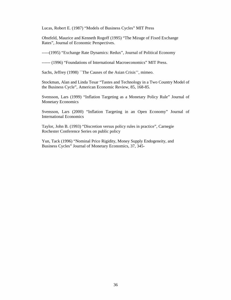
case of the UK, Canada, Mexico and Korea, Table 1 illustrates the results of a

regression of monthly CPI inflation rates on lagged exchange rate changes vis a vis

the US dollar. For Canada and the UK, the lagged exchange rate change has no

explanatory power, at the monthly frequency, for CPI inflation. But for Mexico and

Korea, the coefficient on lagged exchange rate changes is highly significant. The

pass-through for Mexico is over 10 percent, but smaller for Korea. Thus, our

working hypothesis is that exchange rate pass-through is very fast for emerging

markets, but slow for advanced economies.

How does this change the nature of the monetary policy making problem?

Much of the literature on monetary policy in open economies (Svensson 2000, Ball

1998, 2000) has been based on the premise that the rate of CPI inflation is

instantaneously affected by movements in exchange rates. For policymakers

concerned about inflation, this represents both an opportunity and a constraint on

optimal monetary policies. But from the discussion in the last paragraph, we suggest

that this hypothesis is not wholly accurate, except for emerging market economies.

4

Our methodology is to compare the properties of a series of different monetary

rules, in face of exogenous external shocks to the small economy1. Two types of

`Taylor rules’ are introduced, one which partially targets the nominal exchange rate,

and one a standard Taylor rule. We also examine a rule which stabilizes the domestic

rate of CPI inflation (strict inflation targeting), and a rule which pegs the exchange

rate. Finally, we examine the properties of a rule which stabilizes the rate of non-

traded goods inflation. This is the two-sector open economy analogue to the optimal

monetary rule identified by Goodfriend and King (1997), in that it eliminates all

variability in the real marginal cost for non-traded firms, and therefore attains the

equilibrium of the hypothetical economy without nominal rigidities.

The main result that comes out of the analysis is that the trade-off between

exchange rate regimes (or monetary policy rules) may be quite different for an

emerging market economy with very high exchange rate pass-through than for an

advanced economy with limited short-run exchange rate pass-through. In the

emerging market case, a flexible exchange rate rule (such as the Taylor rule, or the

rule that stabilizes non-traded inflation) will help to stabilize the real economy, in face

of external shocks. By facilitating adjustment in both the real exchange rate and real

interest rate, these rules can cushion the economy from the impacts of external

shocks. We find that the best rule to achieve this is the mark-up-stabilization rule.

But in order to stabilize GDP and consumption, the rule has to allow a high volatility

in the nominal exchange rate, and therefore high inflation volatility. There is a clear

trade-off between output/consumption volatility and inflation volatility. If the

1 Monacelli (1999) has also contrasted monetary policy rules in an open economy with full pass-through to those with imperfect pass-through. Our model differs in a number of ways. We focus on a two sector `dependent economy’ model. We look at a wider range of shocks, and allow for a wider range of monetary policy rules, including fixed exchange rates. We also directly compare welfare across the different exchange rate regimes, as well as calibrating our model to the case of emerging market economies.

5

authorities are concerned with consumer price inflation2 (over and above non-traded

goods inflation), then the flexible exchange rate regime brings some costs as well as

benefits. Moreover, the same logic implies that a policy of strict inflation targeting is

quite undesirable in an open economy, since it effectively amounts to a requirement of

fixing the exchange rate. It stabilizes inflation at the expense of a lot of output

instability.

The situation is quite different when pass-through is limited. We model this

process by assuming that foreign firms follow a practice of setting prices in domestic

currency, and only gradually adjusting to exchange rate changes. In this environment,

we find that there is no trade-off between output volatility and inflation volatility. In

fact, a flexible exchange rate can deliver lower output variance and lower inflation

variance than a fixed exchange rate regime. The mark-up-stabilization rule minimizes

the variance of output, consumption, and inflation, among all the rules considered.

The explanation of these results is easy to see. When exchange rates changes

do not fully impact on consumer prices, then external shocks which cause exchange

rate movements have a smaller effect on internal relative prices facing households,

and a smaller effect on domestic inflation. As a result, both inflation and the real

economy tend to be stabilized. At the same time, since exchange rates still

immediately affect interest rates (through UIRP), the monetary policy rule under

flexible exchange rates can still use nominal exchange rates to help stabilize the

economy. Thus, in effect, the exchange rate can be used without inflationary

consequences. The conclusion is that the monetary policy problem is much more

favourable in an economy with limited pass-through, and in this tilts the balance

strongly towards floating exchange rates.

2 Strictly speaking, in our model, there is no reason that consumers should be concerned with CPI

6

A corollary of these findings is that a policy of strict inflation targeting is

much less costly in an economy with limited pass-through, since inflation can be

stabilized while still allowing for a considerable degree of nominal exchange rate

volatility.

A general finding of the paper, in comparing monetary rules, is that the rule

that stabilizes non-traded goods price inflation performs the best. It is a simple,

coherent rule, and just says that the authorities should not pay attention directly to the

exchange rate or traded goods prices in setting interest rates3. There is also an added

attractive feature of the rule. A Taylor type rule in an open economy may be

destabilizing in the presence of `internal shocks’ to the monetary policy decision

making structure. If we thought of such shocks as related to `credibility’ or `risk-

premium’ shocks, then there might be a case for a currency board or a dollarization in

order to eliminate this type of instability. But the rule which stabilizes non-traded

goods price inflation also automatically neutralizes such internal `monetary policy’

shocks. To the extent that such a rule can be made credible, it has an advantage over

a pegged exchange rate, since it also helps to stabilize the economy in face of external

shocks.

The paper is organized as follows. The next section develops the basic model,

which is a two-sector dynamic small open `dependent economy’ model. The model is

calibrated and simulations reported in Section 3. Section 4 discusses the difference

between alternative monetary rules for the volatility of inflation, output, and other

inflation, if the inflation rate of non-traded goods is stabilized. Realistically, however, it is highly likely that central banks will be concerned more generally with CPI inflation. 3 There is a parallel between a non-traded goods inflation rule and the central bank practice of focusing on `core inflation’, excluding goods whose prices display high short term volatility. To the extent that these goods, such as food and energy, are imported, the focus on non-traded goods inflation and core inflation may lead to similar results.

7

variables, and discusses welfare comparisons across regimes. Some conclusions

follow.

8

Section 2.

Here we describe the model of a small open economy that will be used to

compare alternative monetary policy rules. The structure is a very standard two

sector ‘dependent economy’ model. Two goods are produced: a domestic non-traded

good, and an export good, the price of which is fixed on world markets. This is

probably the best representation of the macroeconomic environment of `emerging

market’ economies. Although the real exchange rate is determined by domestic

macroeconomic equilibrium, the economy has no international market power in

traded goods.

A central aspect of the model is the presence of nominal rigidities. Price

stickiness introduces a role for monetary policy and a non-trivial comparison between

exchange rate regimes. But unlike the standard analysis of price stickiness in closed

economy models (e.g. Goodfriend and King 1997, Rotemberg and Woodford, 1997),

in a small open economy prices in the traded goods sector are determined by world

prices. Non-traded goods prices are set in advance by domestic firms however, and

adjust only gradually to shocks.

There are three types of actors in the economy; consumers, firms, and the

monetary authority.

Consumers

The economy is populated by a continuum of consumer/households of

measure unity. The representative consumer has preferences given by

(1) 0 0( , , )t t tt

U E u C H mβ∞

== ∑ ,

where tC is a composite consumption index, such that ( , )t Nt MtC C C C= , where NtC

represents consumption of non-traded goods, and MtC is consumption of an imported

9

foreign good. tH is labor supply, and /t t tm M P= represents real balances, with

tM being nominal money balances, and tP being the consumer price index. Let the

functional form of u be given by

11 1

( , , )1 1 1C H mu C H m

εσ ψ

η χσ ψ ε

−− +

= − +− + −

In addition, if we let composite consumption take the form

1 1 1 11 1 1( (1 ) )t Nt MtC a C a Cρ

ρ ρ ρ ρ ρ− − −= + − , then the implied consumer price index is

11 1 1( (1 ) )Nt MtP aP a Pρ ρ ρ− − −= + − . Finally, assume that consumption is differentiated at the

individual goods level, so that ( )1/(1 )1 1

0( )jt jtC C i di

λλ

−−= ∫ , where 1λ > , j=H,M.

Consumers are assumed not to face any capital market imperfections4.

Therefore, the consumer can borrow directly in terms of foreign currency at a given

interest rate *1ti + for period t. Consumers revenue flows in any period come from their

supply of labour to firms for wages tW , transfers tT from government, profits from

firms in the non traded sector tΠ , return on capital that is rented to firms in each

sector, domestic money, less their debt repayment from last period tD . They then

obtain new loans from foreign capital markets, and use these loans to consume, invest

in new capital, and acquire new money balances. Their budget constraint is thus:

(2) *

1 1

(1 ) ( )t t t t t t Nt Xt t

t t t t t t t t Nt Nt t Xt Xt

PC i S D P I I MW L S D M T PR K PR K+ −

+ + + + += +Π + + + + +

4 Much of the recent post-crisis literature on emerging markets has stressed the imperfections and instability of capital markets. See e.g. Cespedes, Chang and Velasco (2000), Aghion, Bachetta and Banerjee (2000), Devereux and Lane (2000), Cook (2000), and others. But how much this should impact on the monetary policy problem is open to debate. Both Cespedes, Chang and Velasco (2000) and Devereux and Lane (2000) show that introducing collateral constraints on foreign investment financing, and a `currency mismatch’ in balance sheets does not affect the qualitative conclusions with respect to optimal monetary policy in an otherwise conventional model of a small open economy (e.g.

10

Capital stocks in the export and non-traded sectors evolve according to

(3) 1 ( ) (1 )TtXt Xt Xt

Tt

IK K KK

φ δ+ = + −

(4) 1 ( ) (1 )NtNt Nt Nt

Nt

IK K KK

φ δ+ = + −

where the function φ satisfies 0'>φ , and 0'' <φ . This reflects the presence of

adjustment costs of investment. Under this specification, capital cannot move

between sectors at any given time period, but capital in each sector adjusts over time.

The household will choose non-traded and imported goods consumption to

minimize expenditure conditional on total composite demand tC . Demand for non-

traded and imported goods is then

NtNt t

t

PC a CP

ρ−

=

(1 ) MtMt t

t

PC a CP

ρ−

= −

The consumer optimum can be characterized by the following conditions.

(5) 11*

1 1

1(1 )

t tt t t

t t t

S PC E Ci S P

σ σβ− −++

+ +

=+

(6) tt t

t

W C HP

σ ψη=

(7) 1(1 )htt t t

t

M C E dP

εσχ

−−

+

= −

(8) ( )

1 11 1

1

(1 '( ) )'( ) 't Nt Nt

t t NtNt Nt

C i iE C Ri i

σσ δ ϕβ

ϕ ϕ

−− + +

+ ++

− += +

(9) ( )

1 11 1

1

(1 '( ) )'( ) 't Tt Tt

t t XtTt Tt

C i iE C Ri i

σσ δ ϕβ

ϕ ϕ

−− + +

+ ++

− += +

such as the model here). Cook (2000), however, finds a different result, using an alternative specification.

11

where NtNt

Nt

IiK

= , etc. Equation (5) represents the Euler equation for optimal

consumption. Equation (6) is the labour supply equation, while equation (7) gives the

implicit money demand function. Money demand depends on domestic nominal

interest rates. The domestic nominal discount factor is defined as

(10) 11

1

h t tt

tt

C PdPC

σ

σ

−+

+ −+

= .

Note that the combination of (5) and (10) gives the representation of uncovered

interest rate parity for this model. Finally, conditions (8) and (9) describe the optimal

investment choice for the household, where the consumer separately accumulates

capital stock for use in the non-traded and traded goods sectors.

Production Firms

Production is carried out by firms in the non-traded and export sectors. The

sectors differ in their production technologies. The non-traded sector uses labour and

specific capital to produce. An individual firm i in the non-traded sector has

technology

(11) 1Nit N Nit NitY A K Lα α−= ,

where NA is a productivity parameter.

Traded goods production uses both imported intermediate inputs MtI and domestic

value added tV to produce using the technology

(12) 1 1 11 1

(1 )Xt t MtY V Iφφ

φ φϑ ϑ−− − = + −

.

Domestic value-added is obtained from capital and labour according to

(13) 1t X Xt XtV A K Lγ γ−=

Cost minimizing behaviour then implies the following equations

12

(14) (1 ) Nitt Nt

Nit

YW MCH

α= −

(15) NitNt Nt

Nt

YR MCK

α=

(16)

1

(1 ) t Xtt Xt

Xt t

V YW PH V

φγ ϑ

= −

(17)

1

t XtXt Xt

Xt t

V YR PK V

φγ ϑ

=

,

(18)

1

(1 ) XtIMt Xt

Mt

YP PI

φγ ϑ

= −

where NtMC denotes the nominal marginal production cost for a firm in the non-traded

sector (which is common across firms). Equations (14) and (16) describe the optimal

employment choice for firms in each sector. Equations (15) and (17) describe the

optimal choice of capital. Note that the price of the traded export good is XtP .

Movements in this price, relative to MtP and IMtP , represent terms of trade fluctuations

for the small economy. Finally, equation (18) represents the condition for the optimal

choice of intermediate inputs.

Price setting

Firms in the non-traded sector set prices in advance. Following the method of

Calvo (1983) and Yun (1995), assume that firms face a probability )1( κ− in every

period of altering their price, independent of how long their price has been fixed.

Following standard aggregation results, the non-traded goods price follows the partial

adjustment rule

(19) λλλ κκ −−

−− +−= 11

11 ~)1( NtNtNt PPP

13

where NtP~ represents the newly set price for a firm that does adjust its price at time t.

The evolution of NtP~ is then governed by (the approximation)

(20) 1(1 )Nt Nt t NtP MC E Pβκ βκ += − +! ! .

Taking a linear approximation of (17) and (18), assuming an initial steady state where

the rate of change of NtP is constant, we can derive the familiar forward-looking

inflation equation:

(21) 1Nt t t Ntmcn Eπ λ π += +

where Ttmcn represents the log deviation of real marginal cost in the non-traded sector,

t

Nt

MCP

from its steady state level (of unity). Equation (19) is analogous to the forward-

looking inflation equation in Clarida, Gali and Gertler (1999). The key difference

here is that both marginal costs and inflation are specific to the non-tradeable sector.

Monetary policy Rules

Assume that the monetary authority uses a short term interest rate as the

monetary instrument. Given the interest rate, the money supply will be determined

endogenously by the aggregate demand for money arising from the consumer sector,

(i.e. equation (5)). Thus, the analysis of monetary rules can ignore the money supply,

since it is determined as a residual. It is important however that interest rate rules are

set so as to ensure a unique price level and exchange rate, and to avoid the issue of

`real indeterminacy’ that can arise under some interest rate rules in sticky price

models5. Under all calibrations of the model, as discussed below, a unique

equilibrium is obtained.

The general form of the interest rate rule used may be written as

5See Woodford (1999) for conditions on interest rate rules required for uniqueness in the price level. In addition, see Clarida, Gali, and Gertler (1999).

14

(22) ( ) 1

1 1

1 1 (1 )exp( )1 1

n y sh Nt t t tt l t

Nt n t

P P Y Sd i uP P Y S

π πµ µ µ µ

π π−

+− −

= + + +

where it is assumed that 0, 0, 0, 0.n y sπ πµ µ µ µ≥ ≥ ≥ ≥ The parameter

nπµ allows the

monetary authority to control the inflation rate in the non-traded goods sector around

a target rate of nπ . The parameter πµ governs the degree to which the CPI inflation

rate is targeted around the desired target of π . Then yµ and sµ control the degree to

which interest rates attempt to control variations in aggregate output and the exchange

rate, around their target levels of Y and S , respectively. The term exp( )tu represents

a shock to the domestic monetary rule. We discuss the nature of this in more detail

below.

This function allows for a variety of monetary rules. When 0y sπµ µ µ= = = ,

and nπ

µ →∞ , the monetary authorities pursue a policy of strict inflation targeting in

the non-traded goods sector. From equation (19), we see that this will ensure that the

real mark-up is constant. Intuitively, if the monetary policy acts so as to ensure there

is never any need to adjust prices, then there are no consequences of price stickiness.

This point has been made by Goodfriend and King (1997), and others. Therefore, this

policy will replicate the real equilibrium of an economy with flexible prices.

When 0n sπµ µ= = , the authority follows a form of Taylor rule, where

interest rates are adjusted to respond to deviations of CPI inflation and aggregate

output from some target levels. When 0nπ

µ = , then the authority follows a modified

Taylor rule in which the exchange rate is targeted in addition to CPI inflation and

output. When 0n y sπµ µ µ= = = and πµ →∞ , the monetary authority pursues strict

15

CPI inflation targeting. Finally, when 0n yπ πµ µ µ= = = and sµ →∞ , the authority

follows a pegged exchange rate.

Optimal Monetary Policy

What objective function should the monetary authorities have in this

economy? Speaking generally, the model has a natural welfare index; the expected

utility of households in the small economy. An optimal monetary policy would be

one which maximizes expected utility. But recent literature on the analysis of

monetary policy in dynamic sticky-price general equilibrium models has developed a

more direct approach to the formulation of monetary policy objective functions.

Goodfriend and King (1997) point out that, leaving out issues related to the Friedman

rule (or, equivalently, assuming positive nominal interest rates), an optimal monetary

policy should stabilize the mark-up of prices over marginal costs, (`real marginal

cost’). This is explained as follows. The only way in which a sticky-price economy

differs from a flexible price economy is that the mark-up of price over marginal cost

is variable. With flexible prices, firms would set a constant and time-invariant mark-

up (due to CES utility). A monetary rule which stabilizes the mark-up replicates the

flexible price economy. If the equilibrium of the flexible price economy is Pareto

efficient, then this must represent the optimal monetary rule. In fact, the flexible price

economy will typically not have an efficient equilibrium, due to the presence of

monopolistic competitive pricing. But since the monetary policy rule cannot affect

the average mark-up of price over marginal cost in any case (at least in the linearized

version analysed here), the best rule for monetary policy is to reduce the variance of

the mark-up to zero, thereby replicating the flexible price economy.

Subsequent literature refined this rule (Clarida, Gali and Gertler 1999,

Woodford 1999) by linking movements in the price-cost mark-up to deviations of

16

output from its `potential’ level, or the level that it would attain in a flexible price

economy. Woodford (1999) shows in an economy where price-setting is staggered,

inflation generates an additional welfare loss, independent of the gap between output

and potential output (i.e. the unexploited gains from trade due to sticky prices). This

loss arises from the dispersion in relative goods prices, leading to an inefficient

allocation of resources between sectors. In this framework, Woodford’s analysis

implies that expected utility may be approximated by a quadratic function of output

deviations from potential output, and inflation deviations from zero. Both Woodford

and Clarida, Gali and Gertler (1999) then point out that in the absence of direct shocks

to the pricing equation, an optimal monetary policy would set inflation to zero. This

would stabilize the mark-up of price over marginal cost, as suggested by Goodfriend

and King, and simultaneously keep output at its potential level and reduce the

dispersion of relative prices to zero.

In the present model, in the case of immediate pass-through from the exchange

rate to imported goods prices, a monetary policy rule which ensured a constant price-

cost mark-up for non-traded goods firms would replicate the equilibrium of a flexible

price economy. In this case, an appropriate welfare index would be a combination of

output deviations from potential, and inflation in the non-traded goods sector. This

could be achieved by zero inflation in non-traded goods prices. In the economy with

slow pass-through of exchange rate changes, the situation is more complicated,

because even without sticky prices in the non-traded goods sector, monetary rules can

have real effects through their impact on exchange rates. This may lead the monetary

authority to be more generally concerned with CPI inflation, and nominal exchange

rate variability. But derivation of an welfare objective for monetary policy along the

17

lines of Woodford is quite complicated, due to the presence of investment, the two

sector structure, and imperfect pass through.

Rather than take a stand on the exact form of the monetary authority objective

function, we consider the implications of alternative monetary regimes for volatility in

the major macro aggregates, including, output, consumption, and inflation volatility.

As we see, in some cases we may make inferences about desirable monetary policy

regimes without precise knowledge of the weights that the authority puts on inflation

versus output volatility in its loss function. In addition, we also provide a ranking of

alternative policies using household expected utility.

Local Currency Pricing

The law of one price must hold for both export goods, so that

(23) *Xt t XtP S P= .

For import goods however, we allow for the possibility that there is some

delay between movements in the exchange rate and the adjustment of imported goods

prices. Note that this is still consistent with the constraint that the economy is small,

and without market power in the traded goods sector. The assumption is that foreign

suppliers may choose to follow a pricing policy which stabilizes the prices of imports

in terms of local currency. Domestic consumers however, take the local currency

price of imported goods as given.

Without loss of generality, we may assume that imported goods prices are

adjusted in the same manner as prices in the non-traded sector. That is, a measure

1 *κ− of foreign firms adjust their prices in every period. Thus, the imported good

price index for domestic consumers moves as

(24) 1 1 11(1 *) *Mt Mt MtP P Pλ λ λκ κ− − −−= − +!

18

where MtP! represents the newly set price for a foreign firm that does adjust its price at

time t.

The evolution of MtP! is then governed by (the approximation)

(25) *1(1 *) *Mt t Mt t MtP S P E Pβκ βκ += − +! ! .

The interpretation of (26) is that the foreign firm wishes to achieve an identical price

in the home market as in the foreign market. But it may incur a lag in adjusting its

price. The coefficient *κ determines the delay in the `pass-through’ of exchange

rates to prices in the domestic market. Using the same approach as with equation (20)

and (21),we can derive the familiar inflation equation:

(26) *1ˆ ˆ( )Mt t mt t Mts p Eπ λ π += − +

where Mtπ is the inflation rate in domestically denominated traded goods prices, and

t̂s and *ˆmtp represent the log deviation of the exchange rate and foreign traded goods

prices from steady state.

Equilibrium

In each period, the non-traded goods market must clear. Thus, we have

(27) ( )NtNt t Nt Xt

t

PY a C I IP

ρ−

= + +

.

Equation (27) indicates that demand for non-traded goods comes from consumers,

both for consumption and investment demand. In a similar manner, we may describe

the evolution of the economy’s net debt, tD , as

(28) *1 (1 ) (1 ) ( )Mt

t t t t t Xt Xt t Nt Xtt

PS D S D i P Y a C I IP

ρ−

+

= + − + − + +

Labour market clearing for the household sector implies

(29) Nt Xt tH H H+ = .

19

Finally, to recover the nominal price of non-traded goods and imported goods, we use

the conditions

(30) 1(1 )Nt Nt NtP Pπ −= + ,

(31) 1(1 )Mt Mt MtP Pπ −= + ,

with the initial prices 1NP − and 1MP − being given.

The economy’s equilibrium may be described as the sequence of functions

given by ( )tC θ , ( )tH θ , ( )tS θ , ( )htd θ , ( )N tY θ , ( )X tY θ , ( )X tV θ ( )N tH θ , 1( )N tK θ − ,

( )X tH θ , 1( )X tK θ − , ( )X tI θ , ( )N tI θ , ( )M tI θ ( )Nt tR θ , ( )Xt tR θ ( )N tπ θ , ( )Tt tπ θ ,

( )tmcn θ , ( )tD θ , ( )tW θ , ( )M tP θ , ( )X tP θ , ( )tM θ and ( )Nt tP θ Here tθ is the period t

information set. This represents a system of 25 functions that correspond to the

solutions of the 25 equations (3)-(18), (21), (22) (23), (26), and (27)-(31), given the

the CPI definition, and given the definition of the shock processes (discussed below).

The model is solved by linear approximation using the Schur decomposition

method of Klein (2000).

Section 3: Calibration and Solution

We now derive a solution for the model, by first calibrating and then

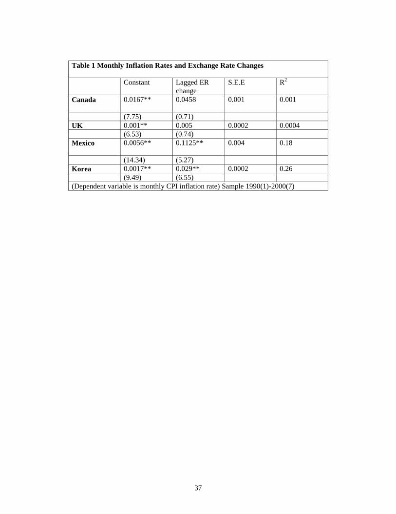
simulating using standard linear approximation techniques. The calibration parameter

values are listed in Table 2. Most values are quite standard. Rather than calibrating

to any single national data-set, we choose a set of `consensus’ parameter values that

are generally applied to developing economies. In some instances, where there is no

direct evidence, we use common parameter assumptions from the macro general

equilibrium literature.

It is assumed that the inter-temporal elasticity of substitution in both

consumption and real balances is 0.5. The consumption inter-temporal elasticity is

20

within the range of the literature, and the equality between the two elasticities ensures

that the consumption elasticity of money demand equals unity, as estimated by

Mankiw and Summers (1986). The elasticity of substitution between non-traded and

imported goods in consumption is an important parameter, on which there is little

direct evidence. Following Stockman and Tesar (1995), we set this to unity. The

elasticity of labour supply is also set to unity, following Christiano, Eichenbaum, and

Evans (1997). In addition, the elasticity of substitution between varieties of

goods determines the average price-cost mark-up in the non-traded sector. Since we

have no direct evidence on mark-ups for emerging market economies we follow

standard estimates from the literature in setting a 10 percent mark-up, so that 11λ = .

Assuming that the economy starts out in a steady state with zero consumption

growth, the world interest rate must equal the rate of time preference. We set the

world interest rate equal to 6 percent annually, an approximate number used in the

macro-RBC literature, so that at the quarterly level, this implies a value of 0.985 for

β .

The factor intensity parameters are quite important in determining the

dynamics of the model. Typically these types of parameters are calibrated in general

equilibrium models by identifying the employment share of GDP. But since it is quite

likely that this share differs across sectors, then it is necessary to obtain separate wage

shares at the sectoral level. We follow Devereux and Cook (2000) in assuming that

the non-traded sector is more labour intensive than the export sector. Specifically, we

take labour share in the non-traded sector to be 70 percent of value added, while

labour export sector value added is 30 percent of value added.

In combination with the other parameters of the model, the parameter a,

governing the share of non-traded goods in the CPI, determines the share of non-

21

traded goods in GDP. Typically, this is significantly smaller for open developing

economies than for OECD economies. Devereux and Cook (2000) and Devereux and

Lane (2000), estimate, for Malaysia and Thailand, that the share of non-traded goods

in total GDP is 55 percent and 54 percent, respectively. For Mexico, Schmitt and

Uribe (2000) estimate a share of 56 percent. Roughly following these studies, we set a

at .5 to imply a share of non-traded goods to GDP of 50 percent. In addition, we set

the share of imported materials in export production to be equal to that of value-

added, and we assume that the elasticity of substitution between value added and

intermediate imports is 0.5.

To determine the degree of nominal rigidity in the model, the value κ ,

governing the speed of price adjustment in non-traded goods, must be chosen. Again,

in the absence of direct evidence on this, we follow the literature (e.g. Chari, Kehoe

and McGratten 1998), and set κ =0.75, so that prices completely adjust after

approximately 4 quarters. As is standard practice, we set the adjustment cost of

capital (elasticity of Tobin’s q with respect to the investment-capital ratio) so as to

imply a standard deviation of investment relative to GDP in a reasonable range.

The degree to which exchange rate and foreign price shocks are `passed-

through’ to domestic imported goods prices is governed by the parameter *κ . As

discussed above, this is a difficult parameter to pin down empirically. Estimates of

pass-through of exchange rate changes to imported goods prices tend to be different

than the observed effects of exchange rate changes on more aggregated price indices.

For instance, Goldberg and Knetter (1997) estimate that the median rate of pass-

through in the US is 50 percent for US manufacturing industries. But other macro

evidence for the US suggests the virtual absence of any effects of exchange rate

changes on domestic goods prices (Engel 2000). Similarly Engel and Roger’s (1996)

22

study suggests little short run effects of exchange rate changes on relative goods

prices between the US and Canada. Similar evidence has been established for

European countries (Engel and Rogers 1999). This suggests that there is a

considerable degree of `local-currency pricing’ in traded goods industries in OECD

countries. Within the structure of the present model, this evidence would suggest that

*κ is positive – foreign exporting firms do not immediately adjust their prices to

exchange rate changes. In the absence of very precise estimates of *κ we follow a

rule of thumb in setting *κ κ= for our calibration of an advanced economy. The

rationalization for this number is that it accords with Engel’s (2000) finding that for

the US and its major industrial trading partners, there is virtually no difference in the

characteristics of the prices of traded and non-traded goods.

On the other hand, as suggested above, the pass-through from exchange rates

to prices is likely to be much higher for emerging markets. Evidence from the Asian

and Mexican crises indicate a very rapid transmission of exchange rate depreciation to

imported goods prices. Again, however, precise estimates of the extent of pass-

through have not been obtained. To fix ideas, we make the extreme assumption that

the pass-through is immediate for our calibrated `emerging market’ economy. Thus,

we set * 0κ = for the emerging market model. Therefore, the law of one price obtains

at all times. Both foreign price shocks and exchange rate changes have immediate

implications for local prices of imported goods.

Shocks

The model implies that the economy is exposed to three types of external

shocks: a) shocks to foreign prices, b) shocks to the foreign interest rate, and c) terms

of trade shocks. The first and third shocks are obviously inter-related. Conceptually,

however, there is a difference between balanced movements in the world price level,

23

and shocks to the relative price of the domestic country export good. We let price

shocks be represented by equal shocks to all foreign prices, i.e. to *MtP and *

XtP and

*IMtP . Terms of trade shocks are represented by shocks to

*

*Xt

Mt

PP

and *

*Xt

IMt

PP

. Since in

the model, shocks to these last two variables have almost identical effects, we assume

that they are equivalent. Thus, the consumer and producer import price indices are

assumed the same.

In the following section we will measure the size of these shocks for a group

of Asian countries. At present, we wish to give an intuitive account of the basic

properties of the model when subjected to each external shock.

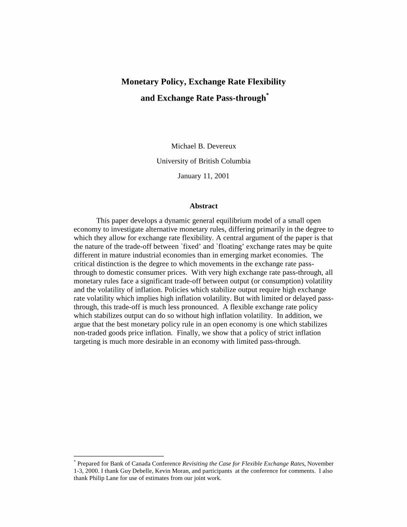
The impact of external shocks under alternative monetary regimes We now illustrate the workings of the model in response to the different external

shocks, under each monetary rule. The monetary rules are categorized in Table 3.

The mark-up rule stabilizes the rate of inflation in non-traded goods, as discussed

above. Two `Taylor-type’ rules are also discussed, one of which targets the exchange

rate. Finally, there is a strict CPI inflation targeting rule, and a pegged exchange rate

rule.

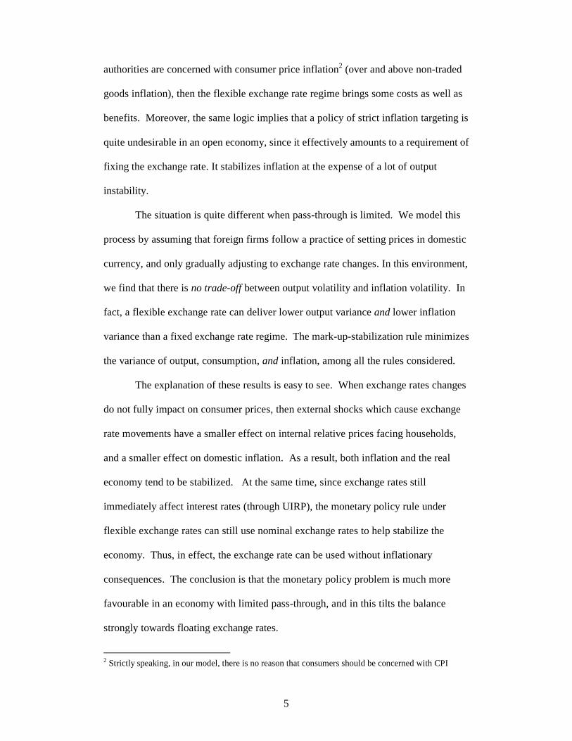
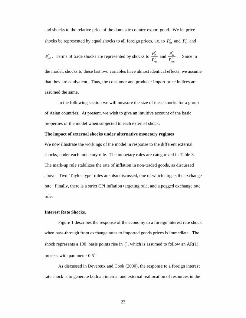
Interest Rate Shocks.

Figure 1 describes the response of the economy to a foreign interest rate shock

when pass-through from exchange rates to imported goods prices is immediate. The

shock represents a 100 basis points rise in *ti , which is assumed to follow an AR(1)

process with parameter 0.56.

As discussed in Devereux and Cook (2000), the response to a foreign interest

rate shock is to generate both an internal and external reallocation of resources in the

24

economy. The interest rate disturbance reduces domestic absorption, generating a

current account surplus. The fall in absorption also forces a real exchange rate

depreciation, leading to a reallocation of factors from non-traded towards export good

production. Thus, there is both an internal and external `transfer’. For all monetary

policy rules, the same phenomenon is observed; absorption falls, the trade balance

improves, and overall GDP falls.

But the magnitude of the response to an interest rate disturbance is affected

quite strongly by the monetary rule. The response of the economy under a strict

inflation target and a pegged exchange rate regime is almost the same. Domestic

absorption falls by much more than under the mark-up rule, or the two Taylor rules.

Under the pegged exchange rate or the strict inflation target, the inflation rate is

effectively stabilized. This means that the domestic real interest rate rises by the same

magnitude as the exogenous foreign interest shock. On the other hand, the other

three rules make use of the nominal exchange rate variability to cushion the real

interest rate impact of the changes. The mark-up rule allows an immediate but

transitory nominal exchange rate depreciation, which generates an expected

appreciation. This dramatically limits the magnitude of the nominal interest rate rise.

While the anticipated appreciation translates into an anticipated rate of CPI deflation,

this is of a smaller magnitude than the anticipated appreciation itself. Figure 1g

establishes that at the time of the shock, there is an expected real exchange rate

appreciation, which reduces the real interest rate impact of the shock. But the

expected real appreciation is much less for the fixed exchange rate rule and the price

stability rule.

6 The shocks are calibrated more directly in the computation below.

25

A clear implication of Figure 1, however, is that the monetary rules which

provide stability in the real economy do so at the expense of inflation stability. The

mark-up rule completely stabilizes the inflation rate in the non-traded goods sector,

but requires high variability of the nominal exchange rate, and therefore generates a

highly volatile overall price level. There is a trade-off between output stability and

inflation stability. The trade-off can be seen most clearly by comparing the simple

Taylor rule with the Taylor rule that includes an exchange rate response. The latter

achieves a lower response of inflation, but at the expense of a higher first period fall

in GDP.

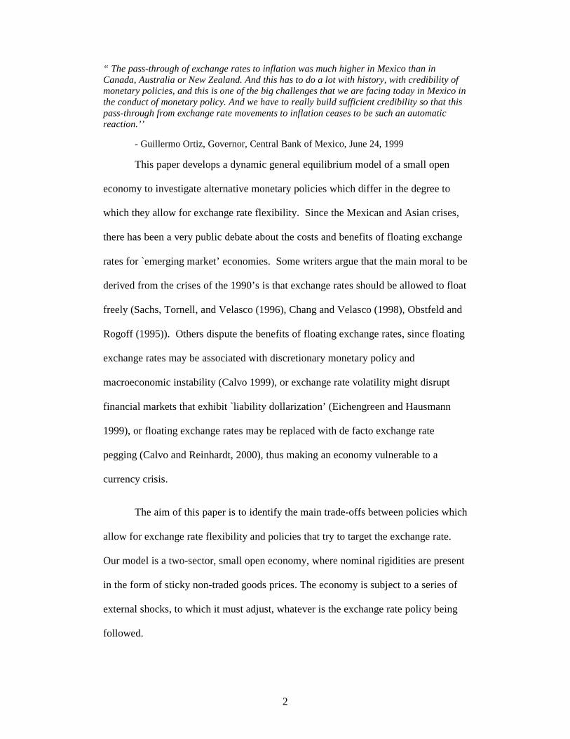
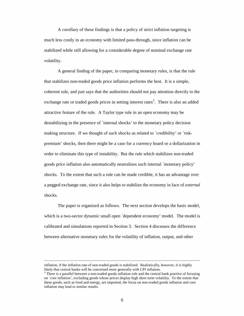
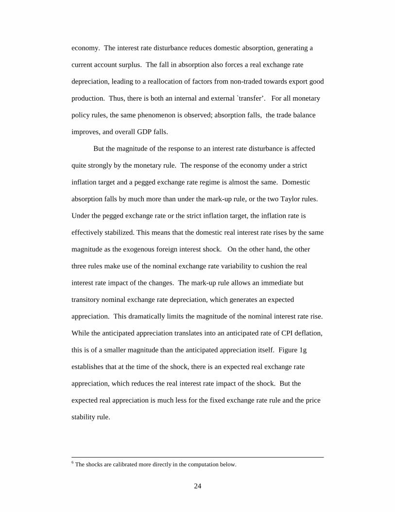
Figure 2 illustrates the case of delayed pass-through. With delayed pass-

through, changes in exchange rates feed into the consumer price index only at the rate

of overall price adjustment. Under the case of fixed exchange rates, the degree of

pass-through is irrelevant, so the results are identical to those in Figure 2. But for the

mark-up rule, and the two versions of the Taylor rule, the effect of the lower pass-

through is to stabilize the rate of inflation. Under the mark-up rule, the movement in

inflation is only 10 percent of the movement with immediate pass through. This acts

to stabilize the real economy, in two ways. First, the muted impact on internal

relative prices reduces the degree of expenditure switching, and leads to a smaller

contraction in non-traded goods production. But, in addition the lower response of

inflation now allows for a lower real interest rate response to the foreign interest rate

shock. Under the mark-up rule, for instance, the expected rate of deflation in the

period of the shock is much less than in the immediate pass-through model. This

cushions the real interest rate response.

A further implication of the limited pass-through model is that it opens up a

substantial difference between a price stability rule and the pegged exchange rate rule.

26

The aggregate CPI can now be stabilized while still allowing significant movement in

the nominal exchange rate. This implies, from Figure 2, that the goal of price stability

is still consistent cushioning the nominal and real interest rate response to the shock.

As a result, absorption and output under the price stability rule are much less variable

than the pegged exchange rate rule.

Note that the flexible exchange rate monetary rules require very large nominal

exchange rate variability. The nominal exchange rate response to the interest rate

shock is higher than in the case of immediate pass-through. Thus, as observed in

previous literature (Betts and Devereux 2000), limited pass-through tends to

exacerbate exchange rate volatility. But it does so with less consequences, since

exchange rates do not immediately feed into CPI inflation.

The conclusion from this case is that in the presence of limited pass-through of

exchange rate changes to import prices, there is no trade-off between output stability

and inflation stability, at least in the response to interest rate shocks. A flexible

exchange rate policy of the type analysed here can cushion the output response to an

external interest rate shock without requiring more inflation instability. In fact, the

(absolute) response of inflation is greater under a fixed exchange rate (which forces a

deflation) than under the flexible exchange rate mark-up rule. Moreover, a rule

following a goal of strict CPI price stability is still consistent with a stabilizing role

for the nominal exchange rate.

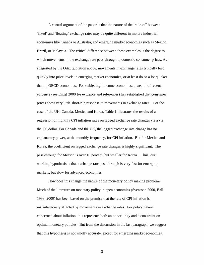
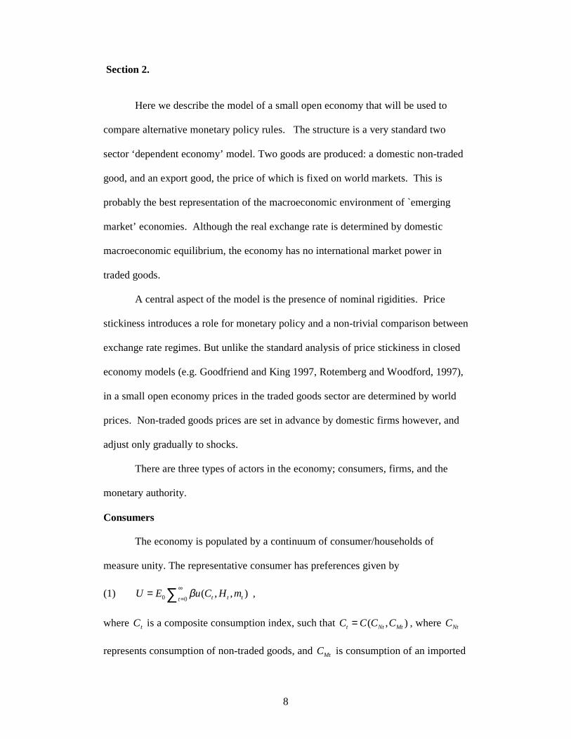
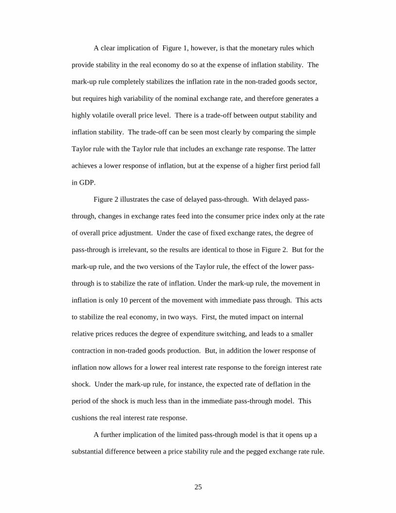
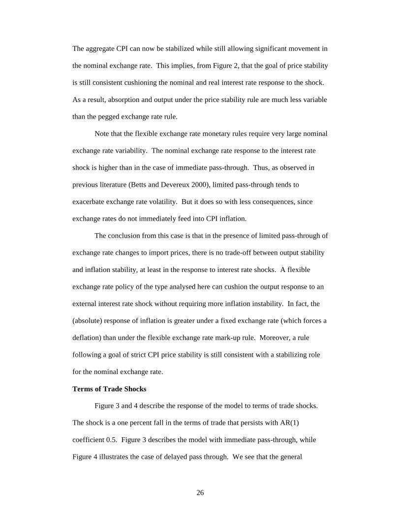
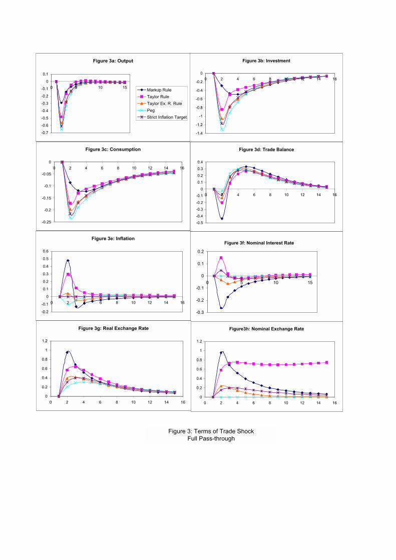
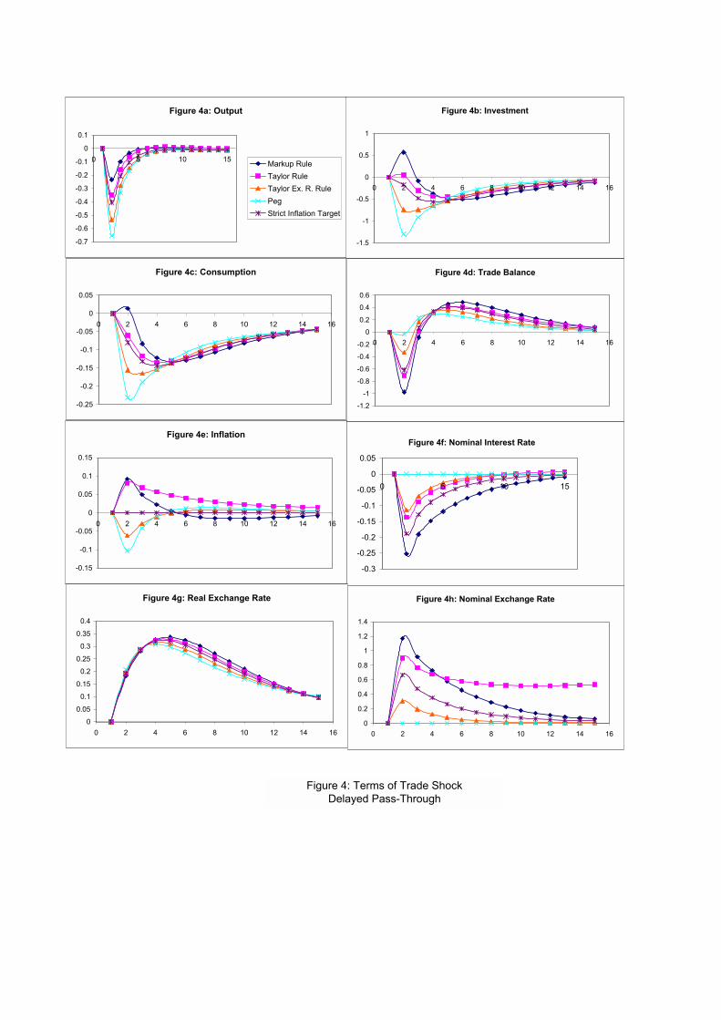
Terms of Trade Shocks

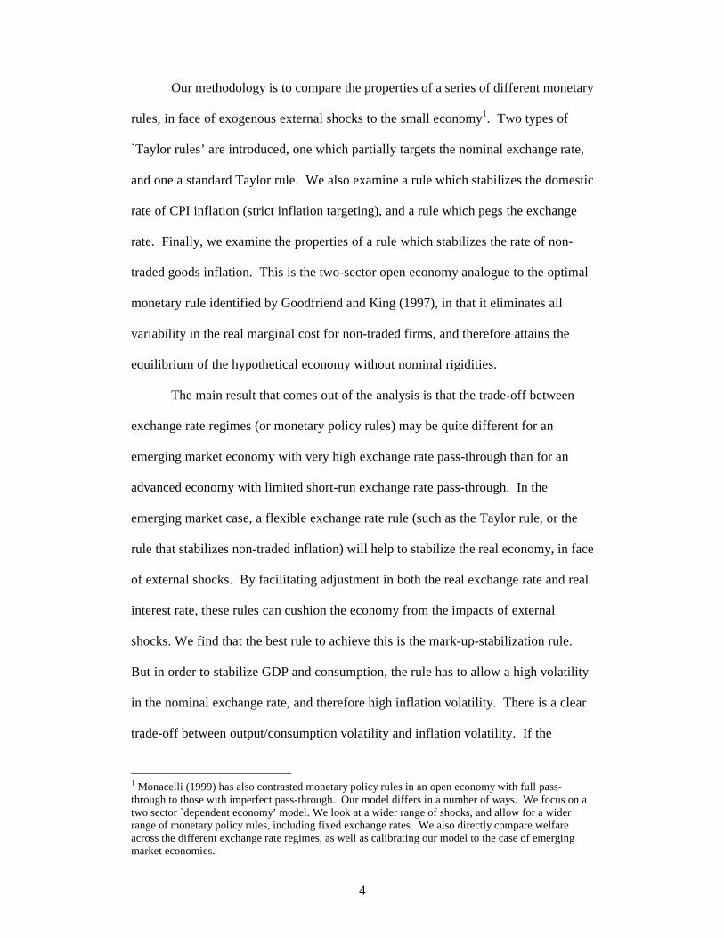
Figure 3 and 4 describe the response of the model to terms of trade shocks.

The shock is a one percent fall in the terms of trade that persists with AR(1)

coefficient 0.5. Figure 3 describes the model with immediate pass-through, while

Figure 4 illustrates the case of delayed pass through. We see that the general

27

conclusions of the previous sub-section apply. With immediate pass-through, the

mark-up monetary rule stabilizes output and absorption, but does so by generating a

high response of the exchange rate and of CPI inflation. The mark-up rule allows for

a sharp, but transitory nominal depreciation. The anticipated appreciation allows for a

fall in the real and nominal interest rate. By contrast, the Taylor rule implies a

persistent nominal depreciation. The nominal interest rate rises, and the real interest

rate is unchanged. Again, the price stability rule and the pegged exchange rate rule

are essentially the same.

With limited pass-through, Figure 4 shows that the real effects of the terms of

trade shock are mitigated, (for all rules except the pegged exchange rate). Given the

very low inflation impact of the nominal depreciation, the Taylor rule becomes much

more expansionary. In fact, all rules except the pegged exchange rate now generate a

fall in the nominal interest rate. In terms of stabilizing output, consumption, and

investment in response to the terms of trade deterioration, the Taylor rule and the

price stability rule are essentially equivalent when there is limited pass-through.

Again, note that the nominal exchange rate responds by substantially more

when there is limited pass-through, while inflation responds by substantially less.

Thus, again, the trade-off between output stability and inflation stability disappears.

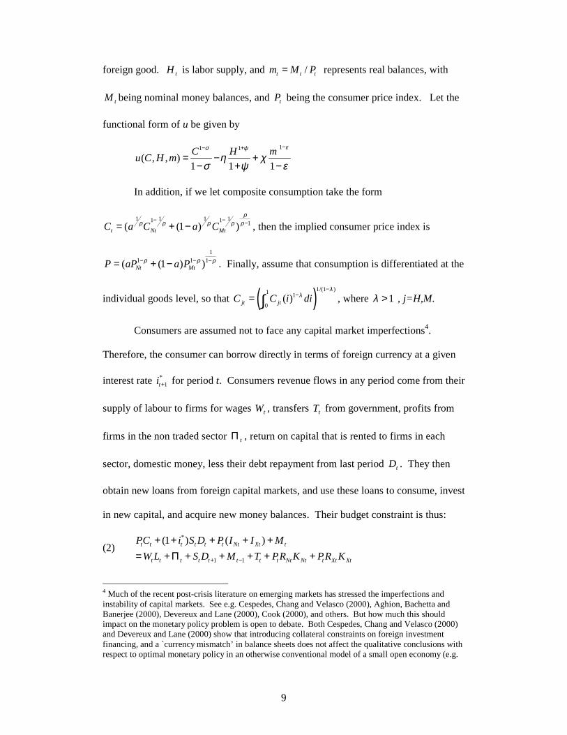
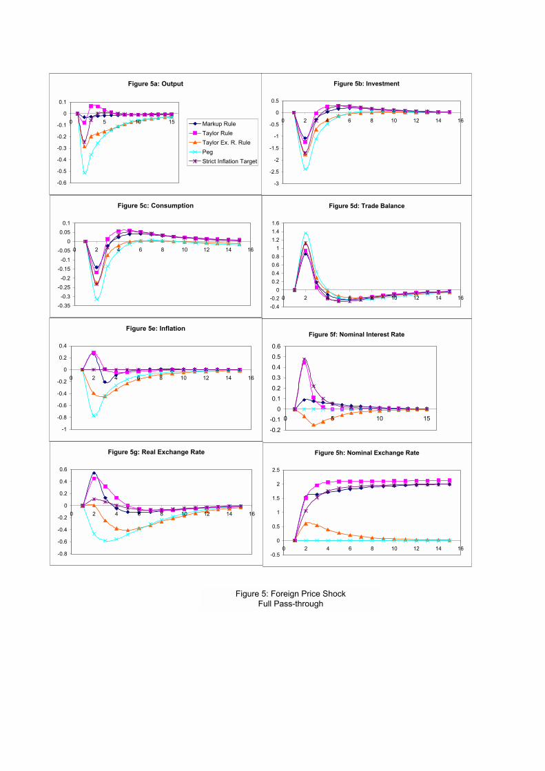
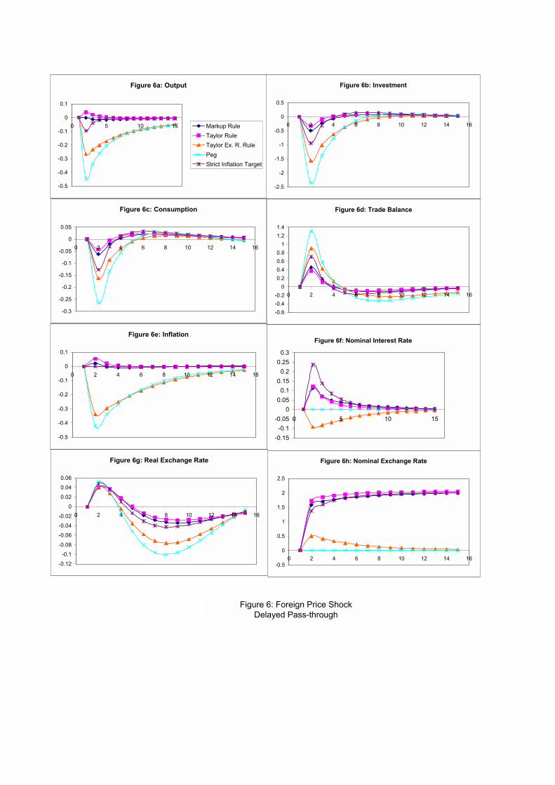
Price Shocks

Figure 5 and 6 illustrate the impact of foreign price shocks. The price shock is

modelled as a shock to the growth rate of foreign goods prices (both export and

import goods), which leaves the terms of trade unchanged. Thus,

letting * *1 1t t tP Pρ ε−∆ = ∆ + , the Figure illustrates the impact of a negative one-unit shock

to tε with 1 0.5ρ = . The effect of this shock can be thought of as a combination of a

28

level shift in the foreign price, and a rise in the foreign real interest rate7. For the

monetary rules which do not concern themselves with the nominal exchange rate

(mark-up, Taylor, and Price Stability Rule), the only impact of the price shock is as a

real interest rate increase. These rules require a permanent increase in the nominal

exchange rate to offset the fall in the foreign price level. But in terms of real effects,

for these rules, the results are the same as in Figure 1 and 2. For the pegged exchange

rate and the Taylor rule with exchange rate response however, the nominal exchange

rate is either kept constant, or is forced to return to its initial position. Both rules

therefore imply a domestic deflation, to restore equilibrium, and both require a greater

fall in output that the other rules. In the case of external price shocks, note that

nominal exchange rate stability is no longer consistent with inflation stability. The

absolute response of inflation is greatest under a pegged exchange rate.

Again, as before, the effect of delayed pass through is to reduce the

inflationary impact of the foreign prices shocks, while also stabilizing the real

economy. Note that even a pegged exchange rate achieves some inflation stability

following a foreign price shock, when pass-through is limited, since the direct impact

of the price shock is not immediately felt in consumer prices.

Internal Shocks

A common criticism of floating exchange rates is that they may be associated

with destabilizing `internal’ shocks arising from domestic monetary policy

uncertainty. In the standard Mundell-Fleming analysis, the presence of domestic

nominal disturbances may tip the balance in favour of an exchange rate peg, since

such shocks can be effectively eliminated by fixing the exchange rate. Recently,

7 To see why the real interest rate must increase, imagine that the nominal exchange rate depreciated to keep the CPI constant in response to the declining path of foreign prices. This would leave the expected inflation rate unchanged, but would imply a positive expected rate of depreciating, increasing the nominal (and therefore real) interest rate.

29

Calvo (1999) and Mendoza (2000) have made the point that monetary policy

instability in Latin America may offer a strong case for the desirability of Currency

Boards or Dollarization.

What does our model imply about the effects of internal shocks? We may

model such shocks as disturbances to interest rates associated with the rule (22). Such

disturbances can be entirely offset by an exchange rate peg, since then the interest rate

must adjust to continually equal the foreign interest rate. By contrast, under a Taylor

rule, such monetary shocks affect real output and consumption.

But the mark-up rule, by stabilizing non-traded goods prices, also completely

insulates the economy from internal shocks to the interest rate process! This is easy

to see. Since the mark-up rule replicates the equilibrium of a flexible price economy,

it supports and economy where monetary neutrality holds. Shocks to the nominal

interest rate process do not affect real interest rates, or any real magnitudes. Thus, the

mark-up rule provides exactly the same insulation from internal interest rate shocks as

does a pegged exchange rate. But since the mark-up rule does a much better job of

insulating the economy from external shocks, it is therefore much preferable to a peg,

at least when the authority does not display an extreme dislike of inflation volatility

(in the case of full pass-through).

Section 4. Quantitative Analysis of the effects of alternative monetary rules.

In this section we investigate quantitative and welfare implications of

alternative monetary rules. This requires us to take a stand on the magnitude and

importance of the shocks. The approach taken is as follows. The interest rate shock

is identified as the US prime rate. This is a reasonably good measure of the `foreign

interest rate’ that is faced by emerging markets. Of course there may be country

specific risk premia affecting the borrowing costs of many emerging markets. Calvo

30

(1999) also suggests that these country risk premia may themselves be related to the

monetary regime – reflecting the degree of perceived international confidence in the

monetary or fiscal regime within a country. But there are significant difficulties in the

measurement of these premia. As a consequence, we abstract from these. While it is

likely that the analysis therefore underestimates the magnitude of interest rate shocks

affecting emerging markets, this would not affect the trade-off between fixed and

floating exchange rates substantially, as greater interest rate volatility would both

increase the stabilization benefits of floating exchange rates, but increase the implied

inflation variability also.

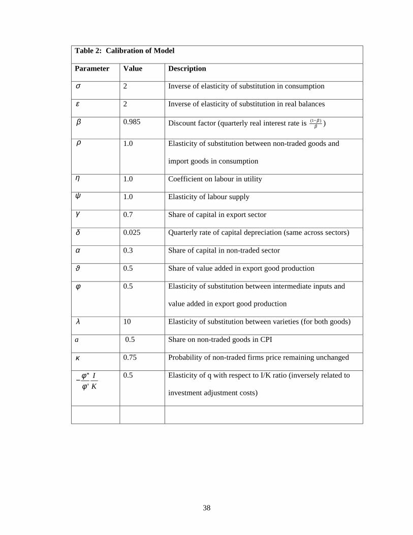
Terms of trade shocks are measured as the ratio of export to import price

deflators. We take an average terms of trade for Asia, from IFS. Finally, we measure

imported goods price shocks as the US dollar price of import goods for Asia, again

from the IFS8. The three variable system, consisting of prime, US dollar import

prices, and terms of trade are estimated as an autoregressive system. The results are

contained in Table 4. These results are then used to calibrate the shock processes for

the model.

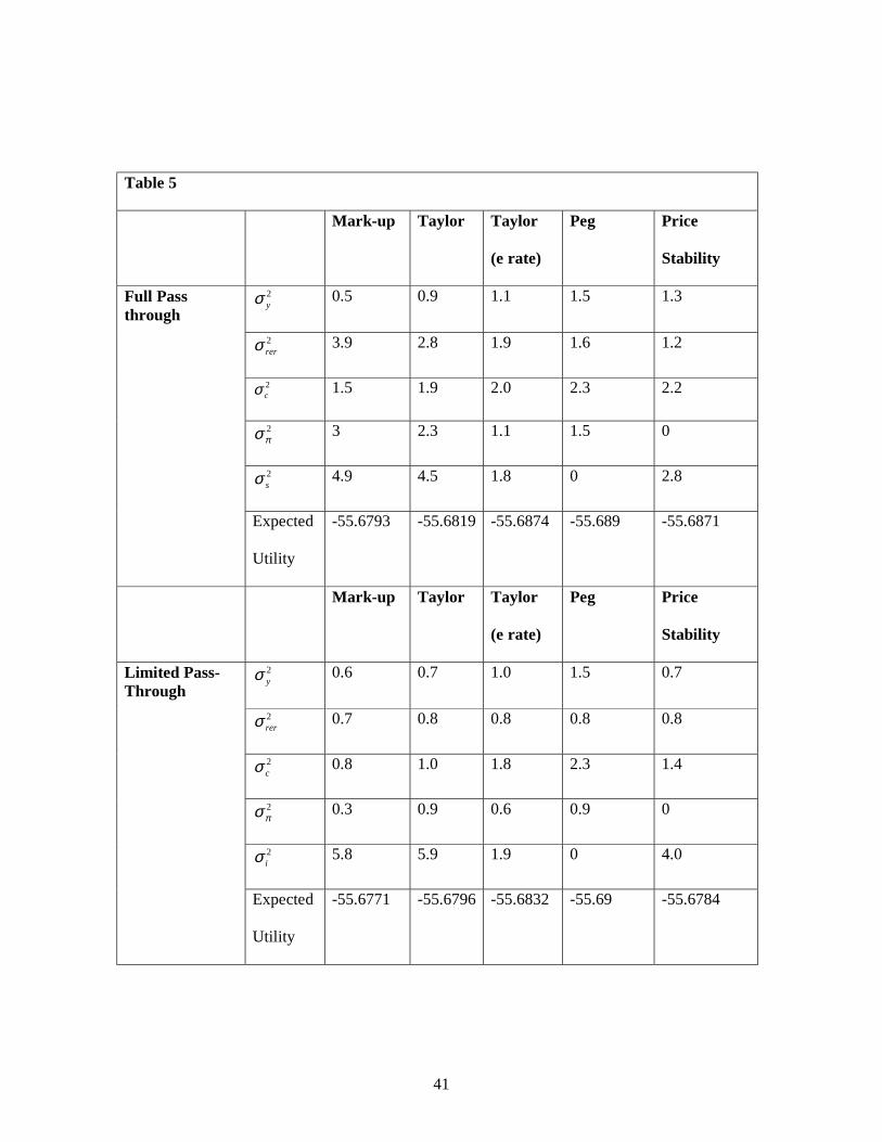
Table 5 illustrates the difference between the various monetary rules for the

volatility of GDP, the real exchange rate, consumption, investment, inflation,

marginal cost, and the nominal exchange rate. The top panel shows the results in the

case of immediate pass-through, while the bottom panel shows the case of limited

pass-through. With full pass-through, there is an inverse relationship between

output/consumption volatility and inflation/nominal exchange rate volatility. The

mark-up rule minimizes output and consumption volatility, but produces very high

inflation and nominal exchange rate volatility. Output and consumption volatility is

31

highest under a pegged exchange rate, but inflation volatility is very small under this

rule. In addition, the difference between a peg and a strict inflation target is quite

small.

The model also suggests that the quantitative effects of exchange rate

flexibility may be substantial. Using a Taylor rule stabilizes output by about 60

percent, and stabilizes consumption by about 18 percent, relative to a fixed exchange

rate. Stabilizing non-traded goods inflation reduces output volatility by two thirds,

and consumption volatility almost by half, although inflation volatility is doubled,

relative to the pegged exchange rate.

When pass-through is lagged, the results are sharply different. Now the rule

that stabilizes non-traded goods inflation minimizes both output/consumption

volatility and inflation volatility. Thus, on this dimension, the mark-up rule dominates

a pegged exchange rate. Output and consumption volatility is lower for the three rules

that do not target the exchange rate. There is also much less of a difference between

the mark-up rule, and Taylor rule, and the Price Stability rule as regards overall output

volatility.

Note that the Table illustrates, as suggested in the previous section, that

nominal exchange rate volatility is much higher with lagged pass-through, for the

`floating exchange rate’ rules. Nominal exchange rate volatility increases by 15 –20

percent in all cases. At the same time, the real exchange rate, measured as the

domestic relative price of non-traded goods, is far less volatile, as both nontraded

prices and export good prices adjust much more slowly in response to all shocks.

Finally, the Table also includes welfare calculations across monetary rules.

These are calculated by averaging repeated draws of utility over 100 quarters,

8 Asia is Hong Kong, India, Indonesia, Korea, Pakistan, Papua NG, Singapore, Sri Lanka, and

32

evaluated at the consumers discount factor9 . In the case of immediate pass-through,

the mark-up rule and the Taylor rule are almost equivalent, although the mark-up rule

results in slightly higher utility. Both rules are clearly better, in utility terms, than the

Taylor rule with exchange rate response, the pegged exchange rate rule, or the price

stability rule. With delayed pass-through, again, the mark-up rule leads (marginally)

to highest utility. Utility is higher in this case for the mark-up rule, the Taylor rule

and the Price Stability rule. Note in addition, that with delayed pass through, the price

stability rule gives utility almost the same as the mark-up rule and the Taylor rule.

Thus, in utility terms, a price stability rule does much better in a regime of limited

pass-through.

These results confirm the general message of the paper; the fixed versus

floating exchange rate trade-off is substantially different in an economy with high

pass-through of exchange rates to traded goods prices than in an economy where pass-

through is delayed. Given that pass-through is likely to be much faster in emerging

markets, for reasons of policy credibility or small size, this makes the choice of fixed

versus flexible exchange rates quite different for emerging markets than for advanced

economies.

Conclusions

We have described the monetary policy trade-off between regimes which

target the exchange rate and those which allow the exchange rate to adjust freely. Our

main result is that the trade-off depends sharply on whether there is a high degree of

pass-through from exchange rates to import good prices. A secondary result is that a

Thailand. 9 As in other literature (e.g. Obstfeld and Rogoff 1995), the utility of real balances are ignored in this calculation. The utility estimates could be transformed into consumption equivalent comparisons across the different policy regimes. But as is well known in this literature (e.g. Lucas 1987), the magnitude of welfare differences across different regimes in business cycle models is extremely small. Thus, we merely report the rankings of utility across regimes.

33

policy of strict inflation targeting is much easier to implement in an economy with

lagged pass-through, since the CPI can be stabilized without destabilizing the real

economy. Finally, we outline a simple and efficient monetary policy rule for an open

economy that is a natural extension of work in the closed economy literature with

sticky prices. This rule is just to stabilize the non-traded goods price level.

34

References

Aghion, Philippe, Philippe Bacchetta, and Abhijit Banerjee 2000 “Currency Crises and Monetary Policy in an Economy with Credit Constraints”, mimeo. Backus, David, Finn E. Kydland, and Patrick J. Kehoe (1992) “International Real Business Cycles”, Journal of Political Economy Ball, Laurence (1998) “Policy Rules for Open Economies” NBER d.p. 6760 ---- (2000) “Policy Rules and External Shocks” NBER d.p. 7910. Bernanke, Ben, Mark Gertler and Simon Gilchrist (1999), "The Financial Accelerator in a Quantitative Business Cycle Model", in John Taylor and Michael Woodford, eds, Handbook of Macroeconomics, Volume 1c. North Holland. Betts, Caroline and Michael B. Devereux (2000) “Exchange Rate Dynamics in a Model of Pricing to Market”, Journal of International Economics, 50. Calvo, Guillermo (1999a), "On Dollarization", mimeo, University of Maryland. Calvo, Guillermo (1999b), "Fixed versus Flexible Exchange Rates", mimeo, University of Maryland. Calvo, Guillermo (1983) “Staggered Prices in a Utility Maximizing Framework” Journal of Monetary Economics, 12, 383-398. Calvo, Guillermo and Carmen Reinhart (2000) ``Fear of Floating’’, mimeo. Cespedes, Luis Felipe, Roberto. Chang, and Andres Velasco (2000) “Balance Sheets and Exchange Rate Policy”, mimeo, Federal Reserve Bank of Atlanta Chang, Roberto and Andres Velasco (1998), "Financial Fragility and the Exchange Rate Regime", NBER Working Paper No. 6469. Chang, Roberto and Andres Velasco (1998), "Financial Fragility and the Exchange Rate Regime", NBER Working Paper No. 6469. Chari, V.V. Patrick J. Kehoe, and Ellen McGratten (1998) “Monetary Shocks and Real Exchange Rates in Sticky Price Models of the International Business Cycle”, Federal Reserve Bank of Minneapolis Research Department Staff Report #223, February. Christiano, Larry J, Martin Eichenbaum and Charles L.Evans (1997) “Sticky Price and Limited Participation Models of Money: A comparison”, European Economic Review 41, 1201-1249. Cook, David (2000) ‘‘Monetary Policy in Emerging Markets’’ Hong Kong University

35

of Science and Technology Devereux, Michael and Philip Lane (2000) “Exchange Rate Regimes and Monetary Policy Rules for Emerging Market Economies”, mimeo, UBC Engel, Charles, 1999, Accounting for U.S. real exchange rate changes, Journal of Political Economy 107, 507-538. Engel, Charles, and John H. Rogers, 1996, How wide is the border?, American Economic Review 86, 1112-1125. Eichengreen, Barry and Ricardo Hausmann (1999), "Exchange Rates and Financial Fragility", NBER w.p 7418. Frankel, Jeffrey (1999), "No Single Currency Regime is Right for All Countries or at All Times", NBER Working Paper #7338. Goldberg Pinelopi and Michael Knetter (1997) Goods Prices and Exchange Rates : What Have We Learned ?, Journal of Economic Literature, 35, pp.1243-1272. Marvin Goodfriend and King, Robert G. (1997) “The New Neo-Classical Synthesis”, NBER Macroeconomics annual. Mendoza, Enrique (2000) “On the Benefits of Dollarization When Stabilization is not Credible and Financial Markets are Imperfect” NBER d.p. 7824. Giovannini, Alberto, Jose De Gregario, and Holger Wolf (1994) “International Evidence on the Price of Non-tradeables”, European Economic Review King, Robert G. and Alexander Wolman (1999) “What Should the Monetary Authority Do when Prices are Sticky?”, in John B. Taylor Ed. Monetary Policy Rules, NBER, University of Chicago Press. Klein, Paul (2000) “Using the Generalized Schur Form to Solve a Multivariate Linear Rational Expectations Model”, Journal of Economic Dynamics and Control, forthcoming. Krugman, Paul (1999), "Balance Sheets, The Transfer Problem and Financial Crises," International Tax and Public Finance, November. Mankiw, N. Gregory and Lawrence Summers (1986) “Money Demand and the Effects of Fiscal Policies” Journal of Money Credit and Banking, 18, 415-429. Mishkin Frederic and Miguel A. Savastano (2000) “Monetary Policy Strategies for

Latin American” NBER w.p. 7617. Monacelli, Tomasso (1999) “Open Economy Policy Rules under Imperfect Pass-

through” mimeo, NYU.

36

Lucas, Robert E. (1987) “Models of Business Cycles” MIT Press Obstfeld, Maurice and Kenneth Rogoff (1995) “The Mirage of Fixed Exchange Rates”, Journal of Economic Perspectives. -----(1995) “Exchange Rate Dynamics: Redux”, Journal of Political Economy ------ (1996) “Foundations of International Macroeconomics” MIT Press. Sachs, Jeffrey (1998) ``The Causes of the Asian Crisis’’, mimeo. Stockman, Alan and Linda Tesar “Tastes and Technology in a Two Country Model of the Business Cycle”, American Economic Review, 85, 168-85. Svensson, Lars (1999) “Inflation Targeting as a Monetary Policy Rule” Journal of Monetary Economics Svensson, Lars (2000) “Inflation Targeting in an Open Economy” Journal of International Economics Taylor, John B. (1993) “Discretion versus policy rules in practice”, Carnegie Rochester Conference Series on public policy Yun, Tack (1996) “Nominal Price Rigidity, Money Supply Endogeneity, and Business Cycles” Journal of Monetary Economics, 37, 345-

37

Table 1 Monthly Inflation Rates and Exchange Rate Changes

Constant Lagged ER change

S.E.E R2

Canada 0.0167** 0.0458 0.001 0.001

(7.75) (0.71) UK 0.001** 0.005 0.0002 0.0004 (6.53) (0.74) Mexico 0.0056** 0.1125** 0.004 0.18

(14.34) (5.27) Korea 0.0017** 0.029** 0.0002 0.26 (9.49) (6.55) (Dependent variable is monthly CPI inflation rate) Sample 1990(1)-2000(7)

38

Table 2: Calibration of Model

Parameter Value Description

σ 2 Inverse of elasticity of substitution in consumption

ε 2 Inverse of elasticity of substitution in real balances

β 0.985 Discount factor (quarterly real interest rate is (1 )ββ− )

ρ 1.0 Elasticity of substitution between non-traded goods and

import goods in consumption

η 1.0 Coefficient on labour in utility

ψ 1.0 Elasticity of labour supply

γ 0.7 Share of capital in export sector

δ 0.025 Quarterly rate of capital depreciation (same across sectors)

α 0.3 Share of capital in non-traded sector

ϑ 0.5 Share of value added in export good production

φ 0.5 Elasticity of substitution between intermediate inputs and

value added in export good production

λ 10 Elasticity of substitution between varieties (for both goods)

a 0.5 Share on non-traded goods in CPI

κ 0.75 Probability of non-traded firms price remaining unchanged

'''

IK

φφ

− 0.5 Elasticity of q with respect to I/K ratio (inversely related to

investment adjustment costs)

39

Table 3: Monetary Rules

nπµ πµ yµ sµ

Mark-up →∞ 0 0 0

Taylor 0 1.5 .5 0

Taylor (e rate) 0 1.5 .5 1

Peg 0 0 0 →∞

Price Stability 0 →∞ 0 0

40

Table 4

VAR estimates: Asia

Variable Prime D(logPm) Dlog(Px/Pm)

Prime(-1) 0.89

(31.1)

-0.002

(-1.61)

0.0

(0.3)

Dlog(Pm(-1) 6.2

(1.97)

0.35

(2.75)

0.047

(0.48)

Dlog (Px/Pm(-1)) 5.63

(1.3)

0.13

0.01

-0.17

(1.3

C 0.88

(3.2)

0.017

(1.59)

-0.003

(-.3)

Residual Covariance Matrix

Prime Dlog(pm) Dlog(Px/Pm)

Prime .3 .0027 .0009

Dlog(Pm) .0027 .00048 -.00017

Dlog(Px/Pm) .001 -.00017 .00028

41

Table 5

Mark-up Taylor Taylor

(e rate)

Peg Price

Stability

2yσ 0.5 0.9 1.1 1.5 1.3

2rerσ 3.9 2.8 1.9 1.6 1.2

2cσ 1.5 1.9 2.0 2.3 2.2

2πσ 3 2.3 1.1 1.5 0

2sσ 4.9 4.5 1.8 0 2.8

Full Pass through

Expected

Utility

-55.6793 -55.6819 -55.6874 -55.689 -55.6871

Mark-up Taylor Taylor

(e rate)

Peg Price

Stability

2yσ 0.6 0.7 1.0 1.5 0.7

2rerσ 0.7 0.8 0.8 0.8 0.8

2cσ 0.8 1.0 1.8 2.3 1.4

2πσ 0.3 0.9 0.6 0.9 0

2iσ 5.8 5.9 1.9 0 4.0

Limited Pass-Through

Expected

Utility

-55.6771 -55.6796 -55.6832 -55.69 -55.6784

!"#$%&'()*+$,-$,

!"#$

!"#%

!"#&

!"#'

!"#(

!"#)

"

"#)

"#(

" % )" )%*+,-./01.234+526,01.234+526,078#01#01.2393:;<,=><0?@A2+<=6@04+,:3<

!"#$%&*'.)*/01&2,3&0,

!&!'#%!'

!(#%!(

!)#%!)

!"#%"

"#%)

" ( & $ B )" )( )& )$

!"#$%&*'4)*5602$3-,"60

!"#$

!"#%

!"#&

!"#'

!"#(

!"#)

"

"#)

"#(

" ( & $ B )" )( )& )$

!"#$%&*'7)*8%(7&*9(:(04&

!)

!"#%

"

"#%

)

)#%

(

(#%

" ( & $ B )" )( )& )$

!"#$%&*'&)*/0;:(,"60

!"#$

!"#&

!"#(

"

"#(

"#&

"#$

"#B

" ( & $ B )" )( )& )$

!"#$%&*';)*<63"0(:*/0,&%&2,*=(,&

!"#(

"

"#(

"#&

"#$

"#B

)

)#(

" % )" )%

!"#$%&*'#)*=&(:*>?4@(0#&*=(,&

!"#&

!"#(

"

"#(

"#&

"#$

"#B

)

)#(

" ( & $ B )" )( )& )$

!"#$%&*'@)*<63"0(:*>?4@(0#&*=(,&

!"#&

!"#(

"

"#(

"#&

"#$

"#B

)

)#(

" ( & $ B )" )( )& )$

C=:.,30)D0?@<3,3E<01+<30;F6>-C.2209+EE!<F,6.:F

!"#$%&'()*'+$,-$,

!"#$

!"#%

!"#&

!"#'

!"#(

!"#)

"

"#)

"#(

" % )" )%*+,-./01.234+526,01.234+526,078#01#01.2393:;<,=><0?@A2+<=6@04+,:3<

!"#$%&'(.*'/01&2,3&0,

!&!'#%!'

!(#%!(

!)#%!)

!"#%"

"#%)

" % )" )% *+,-./01.234+526,01.234+526,078#01#01.2393:;<,=><0?@A2+<=6@04+,:3<

!"#$%&'(4*'5602$3-,"60

!"#$

!"#%

!"#&

!"#'

!"#(

!"#)

"

"#)

"#(

" % )" )% *+,-./01.234+526,01.234+526,078#01#01.2393:;<,=><0?@A2+<=6@04+,:3<

!"#$%&'(7*'8%)7&'9):)04&

!)

!"#%

"

"#%

)

)#%

(

(#%

" % )" )%

*+,-./01.234+526,01.234+526,078#01#01.2393:;<,=><0?@A2+<=6@04+,:3<

!"#$%&'(&*'/0;:),"60

!"#"B!"#"$!"#"&!"#"(

""#"("#"&"#"$"#"B"#)"#)(

" % )" )%

*+,-./01.234+526,01.234+526,078#01#01.2393:;<,=><0?@A2+<=6@04+,:3<

!"#$%&'(;*'<63"0):'/0,&%&2,'=),&

"

"#(

"#&

"#$

"#B

)

)#(

" % )" )%

*+,-./01.234+526,01.234+526,078#01#01.2393:;<,=><0?@A2+<=6@04+,:3<

!"#$%&'(#*'=&):'>?4@)0#&'=),&

!"#)%

!"#)

!"#"%

"

"#"%

"#)

"#)%

" % )" )%

*+,-./01.234+526,01.234+526,078#01#01.2393:;<,=><0?@A2+<=6@04+,:3<

!"#$%&'(@*'<63"0):'>?4@)0#&'=),&

!"#&!"#("

"#("#&"#$"#B)

)#()#&)#$

" % )" )%

*+,-./01.234+526,01.234+526,078#01#01.2393:;<,=><0?@A2+<=6@04+,:3<

C=:.,30(D0?@<3,3E<01+<30;F6>-G32+53H09+EE!<F,6.:F

!"#$%&'()*'+$,-$,

!"#$

!"#%

!"#&

!"#'

!"#(

!"#)

!"#*

"

"#*

" & *" *& +,-./012/345,637-12/345,637-189#12#12/34:4;<=->?=1@AB3,=>7A15,-;4=

!"#$%&'(.*'/01&2,3&0,

!*#'

!*#)

!*

!"#C

!"#%

!"#'

!"#)

"" ) ' % C *" *) *' *%

!"#$%&'(4*'5602$3-,"60

!"#)&

!"#)

!"#*&

!"#*

!"#"&

"" ) ' % C *" *) *' *%

!"#$%&'(7*'8%)7&'9):)04&

!"#&

!"#'

!"#(

!"#)

!"#*

"

"#*

"#)

"#(

"#'

" ) ' % C *" *) *' *%

!"#$%&'(&*'/0;:),"60

!"#)

!"#*

"

"#*

"#)

"#(

"#'

"#&

"#%

" ) ' % C *" *) *' *%

!"#$%&'(;*'<63"0):'/0,&%&2,'=),&

!"#(

!"#)

!"#*

"

"#*

"#)

" & *" *&

!"#$%&'(#*'=&):'>?4@)0#&'=),&

"

"#)

"#'

"#%

"#C

*

*#)

" ) ' % C *" *) *' *%

!"#$%&(@*'<63"0):'>?4@)0#&'=),&

"

"#)

"#'

"#%

"#C

*

*#)

" ) ' % C *" *) *' *%

D>;/-41(E154-FG17B15-,H41<I7?.D/331:,GG!=I-7/;I

!"#$%&'()*'+$,-$,

!"#$

!"#%

!"#&

!"#'

!"#(

!"#)

!"#*

"

"#*

" & *" *& +,-./012/345,637-12/345,637-189#12#12/34:4;<=->?=1@AB3,=>7A15,-;4=

!"#$%&'(.*'/01&2,3&0,

!*#&

!*

!"#&

"

"#&

*

" ) ' % C *" *) *' *%

!"#$%&'(4*'5602$3-,"60

!"#)&

!"#)

!"#*&

!"#*

!"#"&

"

"#"&

" ) ' % C *" *) *' *%

!"#$%&'(7*'8%)7&'9):)04&

!*#)

!*

!"#C

!"#%

!"#'

!"#)

"

"#)

"#'

"#%

" ) ' % C *" *) *' *%

!"#$%&'(&*'/0;:),"60

!"#*&

!"#*

!"#"&

"

"#"&

"#*

"#*&

" ) ' % C *" *) *' *%

!"#$%&'(;*'<63"0):'/0,&%&2,'=),&

!"#(

!"#)&

!"#)

!"#*&

!"#*

!"#"&

"

"#"&

" & *" *&

!"#$%&'(#*'=&):'>?4@)0#&'=),&

"

"#"&

"#*

"#*&

"#)

"#)&

"#(

"#(&

"#'

" ) ' % C *" *) *' *%

!"#$%&'(@*'<63"0):'>?4@)0#&'=),&

"

"#)

"#'

"#%

"#C

*

*#)

*#'

" ) ' % C *" *) *' *%

D>;/-41'E154-FG17B15-,H41<I7?.J43,64H1:,GG!5I-7/;I

!"#$%&'()*'+$,-$,

!"#$

!"#%

!"#&

!"#'

!"#(

!"#)

"

"#)

" % )" )% *+,-./01.234+526,01.234+526,078#01#01.2393:;<,=><0?@A2+<=6@04+,:3<

!"#$%&'(.*'/01&2,3&0,

!'

!(#%

!(

!)#%

!)

!"#%

"

"#%

" ( & $ B )" )( )& )$

!"#$%&'(4*'5602$3-,"60

!"#'%!"#'!"#(%!"#(!"#)%!"#)!"#"%

""#"%"#)

" ( & $ B )" )( )& )$

!"#$%&'(7*'8%)7&'9):)04&

!"#&!"#("

"#("#&"#$"#B)

)#()#&)#$

" ( & $ B )" )( )& )$

!"#$%&'(&*'/0;:),"60

!)

!"#B

!"#$

!"#&

!"#(

"

"#(

"#&

" ( & $ B )" )( )& )$

!"#$%&'(;*'<63"0):'/0,&%&2,'=),&

!"#(!"#)"

"#)"#(

"#'"#&"#%"#$

" % )" )%

!"#$%&'(#*'=&):'>?4@)0#&'=),&

!"#B

!"#$

!"#&

!"#(

"

"#(

"#&

"#$

" ( & $ B )" )( )& )$

!"#$%&'(@*'<63"0):'>?4@)0#&'=),&

!"#%

"

"#%

)

)#%

(

(#%

" ( & $ B )" )( )& )$

C=:.,30%D0C6,3=:@09,=>30;E6>-C.2209+FF!<E,6.:E

!"#$%&'()*'+$,-$,

!"#$

!"#%

!"#&

!"#'

!"#(

"

"#(

" $ (" ($ )*+,-./0-123*415+/0-123*415+/67#/0#/0-12829:;+<=;/>?@1*;<5?/3*+92;

!"#$%&'(.*'/01&2,3&0,

!'#$

!'

!(#$

!(

!"#$

"

"#$

" ' % A B (" (' (% (A

!"#$%&'(4*'5602$3-,"60

!"#&

!"#'$

!"#'

!"#($

!"#(

!"#"$

"

"#"$

" ' % A B (" (' (% (A

!"#$%&'(7*'8%)7&'9):)04&

!"#A!"#%!"#'"

"#'"#%"#A"#B(

(#'(#%

" ' % A B (" (' (% (A

!"#$%&'(&*'/0;:),"60

!"#$

!"#%

!"#&

!"#'

!"#(

"

"#(

" ' % A B (" (' (% (A

!"#$%&'(;*'<63"0):'/0,&%&2,'=),&

!"#($!"#(!"#"$

""#"$"#("#($"#'"#'$"#&

" $ (" ($

!"#$%&'(#*'=&):'>?4@)0#&'=),&

!"#('!"#(!"#"B

!"#"A!"#"%!"#"'

"

"#"'"#"%"#"A

" ' % A B (" (' (% (A

!"#$%&'(@*'<63"0):'>?4@)0#&'=),&

!"#$

"

"#$

(

(#$

'

'#$

" ' % A B (" (' (% (A

C<9-+2/AD/C5+2<9?/8+<=2/:E5=,F21*42G/8*HH!;E+5-9E/