DT. N° 2018-002 Serie de Documentos de Trabajo

Working Paper series Febrero 2018

Los puntos de vista expresados en este documento de trabajo corresponden a los autores y no reflejan

necesariamente la posición del Banco Central de Reserva del Perú.

The views expressed in this paper are those of the authors and do not reflect necessarily the position of the Central Reserve Bank of Peru.

BANCO CENTRAL DE RESERVA DEL PERÚ

Monetary policy spillovers, global commodity prices and cooperation

Andrew Filardo1, Marco Lombardi1 Carlos Montoro2 and

Massimo Ferrari3

1 Bank for International Settlements 2 Banco Central de Reserva del Perú y Ministerio de Economia y Finanzas

3 Università Cattolica del Sacro Cuore

1

Monetary policy spillovers, global commodity prices and cooperation1

Andrew Filardo2, Marco Lombardi2, Carlos Montoro3 and Massimo Ferrari4

Abstract

How do monetary policy spillovers complicate the trade-offs faced by central banks face when responding to commodity prices? This question takes on particular relevance when monetary authorities find it difficult to accurately diagnose the drivers of commodity prices. If monetary authorities misdiagnose commodity price swings as being driven primarily by external supply shocks when they are in fact driven by global demand shocks, this conventional wisdom – to look through the first-round effects of commodity price fluctuations – may no longer be sound policy advice.

To analyse this question, we use the multi-country DSGE model of Nakov and Pescatori (2010) which breaks the global economy down into commodity-exporting and non-commodity-exporting economies. In an otherwise conventional DSGE setup, commodity prices are modelled as endogenously changing with global supply and demand developments, including global monetary policy conditions. This framework allows us to explore the implications of domestic monetary policy decisions when there is a risk of misdiagnosing the drivers of commodity prices.

The main findings are: i) monetary authorities deliver better economic performance when they are able to accurately identify the source of the shocks, ie global supply and demand shocks driving commodity prices; ii) when they find it difficult to identify the supply and demand shocks, monetary authorities can limit the deterioration in economic performance by targeting core inflation; and iii) the conventional wisdom approach of responding to global commodity price swings (as external supply shocks when they are truly global demand shocks) results in an excessive procyclicality of global inflation, output and commodity prices. In light of recent empirical studies documenting a significant role of global demand in driving commodity prices, we conclude that the systematic misdiagnoses inherent in the conventional wisdom applied at the country level have contributed to destabilising procyclicality at the global level. These findings support calls for greater attention to global factors in domestic monetary policymaking and highlight potential gains from greater monetary policy cooperation focused on accurate diagnoses of domestic and global sources of shocks.

Keywords: commodity prices, monetary policy, spillovers, global economy.

JEL classification: E52, E61.

1 We thank conference participants at the Central Bank of Brazil’s XVII Annual Inflation Targeting

Seminar, CEMLA’s XX Annual Meeting and CEBRA’s 2017 Annual Meeting. We also thank seminar participants at the Bank for International Settlements, the Bank of Canada and Bank of Japan for their comments. The views expressed here are those of the authors and do not necessarily reflect those of the Bank for International Settlements, the Central Reserve Bank of Peru.

2 Bank for International Settlements.

3 Central Reserve Bank of Peru and Ministry of Economy and Finance of Peru.

4 Università Cattolica del Sacro Cuore.

2

I. Introduction

Over the past decade, global commodity prices have experienced wide

swings, reaching historically high levels in the run-up to the Great Recession

before plummeting as the global economy collapsed. Prices subsequently

rebounded with the global economic recovery but, more recently, commodity

prices have fallen again amid significant policy concerns. While challenging,

this type of volatility is not a new environment for policymakers. Even though

most commodity prices remained broadly stable during the so-called Great

Moderation, they were quite volatile in the 1970s amid geopolitical tensions

that pushed oil price volatility to then unprecedented levels.

It was the experience of the 1970s that forged the conventional wisdom

about how monetary authorities should respond to commodity price

fluctuations. Commodity price fluctuations were seen largely as the result of

exogenous supply shocks; in such an environment, the conventional wisdom

that emerged was that, when facing such swings, monetary authorities should

look through the first-round price effects and only respond to the second-

round effects on wage and inflation expectations. In practice, this suggested

a monetary policy focus on core inflation.

Views about the drivers of global commodity price swings have been

evolving, especially in recent years, as a growing body of statistical evidence

points to a new interpretation of commodity price swings. Kilian (2009), for

example, finds evidence that oil price fluctuations have been increasingly

influenced by demand from commodity-hungry emerging market economies

(EMEs). The most recent literature has not challenged this view: Kilian and

Baumeister (2016) argue that the oil price decline in 2015 should also be

ascribed to a slowdown in global economic activity; and Stuermer (2017) and

Fukei et al (2018) emphasises the role of demand shocks in a historical

perspective. In a similar vein, Sussman and Zohar (2017) report that

commodity price fluctuations can be taken as a proxy for global demand. In

a broader context, Filardo and Lombardi (2013) note the growing prominence

3

of these global demand shifters for EME inflation dynamics. This new evidence

raises doubts about the relevance of the conventional wisdom and may even

suggest that the exogenous supply shock view is not only misleading but

actually contributing to global economic and financial instability.

The prominence of endogenous commodity price swings has important

implications for monetary policy, given the central role of monetary policy in

influencing aggregate demand. The relationship between monetary policy

decisions and endogenous commodity prices implies an important two-way

link. Monetary policy decisions influence aggregate demand and hence

commodity prices. Indeed, Filardo and Lombardi (2013) and Anzuini et al

(2013) report evidence that loose monetary policy has had an impact on

commodity prices via the global demand channel. 5 At the same time,

commodity price swings influence price stability and hence monetary policy

decisions.

This two-way relationship can operate to stabilise the economy under

certain conditions and de-stabilise the economy under others. For example,

when monetary authorities around the world correctly diagnose the nature of

the shocks driving commodity prices and internalise the monetary policy

spillovers across national borders, monetary policy can be stabilising.

However, when monetary authorities systematically misdiagnose the nature

of the shocks driving commodity prices and largely ignore the spillover effects

of their collective actions, monetary policy at the global level can be

excessively procyclical.

The misdiagnosis risk is particularly high in a world of many central banks

with purely domestic monetary policy mandates. Individual countries may

think that because they are sufficiently small, they can reasonably ignore the

impact of their own policy decisions on the rest of the world. This would be

the case if all economies were hit by uncorrelated idiosyncratic shocks.

5 There is also evidence that US monetary policy may play a special role. Akram (2009) finds that lower

interest rates in the United States boost commodity prices through the exchange rate channel. For further discussion about the importance of US exchange rate spillovers, see Hofmann et al (2017).

4

However, global shocks imply that central banks are likely to respond in a

correlated way. So, in the case of a global demand shock, country-level

monetary policy responses highlight the potential for a fallacy of size, ie when

monetary authorities respond in a similar way to global shocks, the collection

of monetary authorities effectively act as if they were a large monetary

authority.

The fallacy of size and the potential role of misdiagnosing the drivers of

commodity prices also cast light on the shortcomings of the current

international monetary system. In this context, questions are being raised

about whether monetary authorities are sufficiently internalising monetary

policy spillovers and spillbacks. The failure to do so would contribute to both

economic and financial stability concerns (Rajan (2014) and Caruana et al

(2014)).

From a modelling perspective, this discussion suggests the importance of

developing monetary policy models encompassing endogenous commodity

prices and monetary authorities that are subject to misdiagnosis risk. To date,

the bulk of the theoretical literature has stayed clear of models with

endogenous commodity prices (see eg Leduc and Sill (2004), Carlstrom and

Fuerst (2006), Montoro (2012), Natal (2012) and Catao and Chang (2015)).

Moreover, this literature has generally focused on how a monetary authority

should respond to exogenous movements in oil prices, eg whether it is

optimal to target core or headline inflation and whether commodity price

movements have far-reaching implications for the trade-off between

stabilising output and controlling inflation. For example, Blanchard and Gali

(2010) have gone so far as to argue that an increase in commodity prices

driven by foreign demand can still be treated by a domestic monetary

authority as an external supply shock. Such a conclusion is less tenable in

models of endogenous commodity prices and correlated monetary policy

reaction functions.

Various theoretical papers have addressed the endogeneity of

commodity prices in small-scale DSGE models (eg Backus and Crucini (1998),

5

Bodenstein et al (2011) and Nakov and Nuño (2013)). However, these models

have generally ignored monetary policy, focusing instead on oil price

determination and the frictions affecting it. Nakov and Pescatori (2010) is an

early attempt to characterise monetary policy trade-offs in a DSGE model in

which oil prices are determined endogenously. Another important

contribution to this literature is Bodenstein et al (2012), who highlight, as we

do, the importance of identifying the nature of the shocks hitting the

economy.

Our model extends this class of models by considering the policy

challenges facing a monetary authority when it tries to infer the source of

commodity price shocks.6 Namely, there is a risk that a monetary authority

may misdiagnose a commodity price swing as being driven by an external

supply shock when it is, in fact, driven by an endogenous global demand

shock, and vice versa. In our model, the commodity price is endogenously

determined in equilibrium by the interplay of global demand from a

commodity-importing country (or region) and commodity supply from two

types of commodity-exporting country – one competitive and one

monopolistic. In this setting, the optimal monetary policy response to

commodity price swings depends on the perception of the underlying drivers

of the swings. Unable to fully know the nature of the drivers, the monetary

authority infers them via signal extraction, leaving open the possibility of

systematic misdiagnosis. The nature and implications of misdiagnosis risk are

addressed.

The modelling exercise highlights several policy-relevant implications.

First, it is important to distinguish between global demand and supply shocks

when a monetary authority responds to commodity prices. The optimal

responses to global demand and supply shocks are different. On the one

hand, the optimal response to demand shocks is to lean against them fully, a

result consistent with a standard New Keynesian closed economy model. On

6 See Filardo and Lombardi (2013) for a discussion of commodity price misdiagnosis risks in the context

of Asian EMEs.

6

the other hand, the optimal response to commodity supply shocks (ie a

decrease in commodity prices) is to look through them.

Second, by looking through the impact on headline inflation, monetary

policy does not perfectly stabilise core inflation. In other words, the

conventional wisdom of looking through the first-round effects of commodity

price swings is not optimal in our model. This is because our model breaks

the “divine coincidence” between inflation and output gap stabilisation (eg

Blanchard and Gali (2007)), which is a standard feature of DSGE models with

exogenous commodity prices. In part, the breaking of such a divine

coincidence comes from the assumption of a monopolistic commodity

exporter that sets prices by assuming a downward sloping demand curve.

Third, misdiagnosis risk matters in monetary policy. In the case where the

monetary authority misinterprets supply-driven increases in commodity

prices as demand-driven, the contraction in both output and core inflation is

larger than in the case of an accurate diagnosis. This outcome indicates

another reason for the breakdown of the divine coincidence in this model

(even if the dominant exporter acts as a price taker). This finding underscores

the importance of correctly diagnosing the underlying sources of commodity

price swings when setting monetary policy. For example, when commodity

price fluctuations are driven by global demand shocks, a monetary authority

that consistently misdiagnoses them as external supply shocks amplifies

cyclical fluctuations and, as a result, destabilises the economy.

Of course, in any uncertain environment, there is a risk that shocks will be

misdiagnosed. But in the case of correlated global shocks and domestically-

oriented monetary policy mandates, the risk is particularly high. When facing

global commodity price swings, there is a natural tendency for a given

monetary authority – even in a relatively large country – to treat them as if

they were exogenously-determined external supply shocks. Clearly, one lone

monetary authority has little, if any, impact on global prices. However, if a

sufficient number of monetary authorities were to act in a similar (and

uncoordinated) way, their joint behaviour would result in procyclical effect

7

that could destabilise the global economy. This coordination failure supports

the case for greater central bank cooperation in a world experiencing wide

endogenous commodity price swings.

II. The model

We present a global economic model in which commodity prices are

determined endogenously, in the spirit of Nakov and Pescatori (2010).7 The

global economy is split into commodity importers and exporters. The

commodity-importing region is treated as one representative country (but

this can be extended to a group of importing countries without loss of

generality). The commodity-importing country does not produce the

commodity itself but uses it both as a consumption good and as an input into

the production of final goods. Final goods producers in the commodity-

importing country are subject to monopolistic competition and nominal

rigidities, and the central bank sets monetary policy using a linear policy rule

à la Taylor (1993).

The commodity-exporting region is made up of a dominant commodity-

exporting country and a fringe of smaller competitive exporters. These

countries produce the commodity using final goods sold by the commodity-

importing region. In addition, the commodity-exporting countries buy final

goods for their consumption from the commodity-importing country.

On the supply side, the dominant commodity-exporting country has

market power and sets prices above marginal cost. The fringe of small

exporting countries is similar in structure to the dominant exporting country

7 Our model deviates from the setup of Nakov and Pescatori (2010) in four key respects in order to

better characterise the monetary policy trade-offs: i) we introduce the commodity good into the households’ utility function, which can drive a wedge between headline and core inflation in the commodity-importing country; ii) we interpret the commodity as a broad basket of commodities rather than focusing narrowly on oil; iii) we solve the Nash problem for the dominant producer, versus the Ramsey problem, so as to reflect realistic information constraints; and iv) we introduce the possibility of misdiagnosis risk by the monetary authority of the commodity-importing country, which by itself breaks the divine coincidence property of the model.

8

but operates competitively, taking commodity prices as given. Note that

nominal rigidities are absent in the commodity-exporting countries, thereby

simplifying the modelling of monetary policy trade-offs; in this model, there

is only a role for a monetary authority to conduct countercyclical policy from

the perspective of the commodity-importing country.8

The rest of this section provides the modelling details.

II.1. Commodity-importing countries

II.1.1 Households

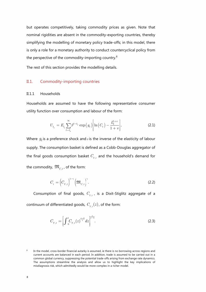
Households are assumed to have the following representative consumer

utility function over consumption and labour of the form:

( ) ( )1

exp ln ,1

o

o o

o

vt t t

t t t tt t

LU E g C

vb

¥ +-

=

é ùê ú= -ê ú+ê úë û

å (2.1)

Where tg is a preference shock andv is the inverse of the elasticity of labour

supply. The consumption basket is defined as a Cobb-Douglas aggregator of

the final goods consumption basket ,Y t

C and the household's demand for

the commodity, ,C tM , of the form:

( ) ( )1

, ,.

t Y t C tC C

g g-

= M (2.2)

Consumption of final goods, ,Y t

C , is a Dixit-Stiglitz aggregate of a

continuum of differentiated goods, ,( )

Y tC z , of the form:

1

, ,0

11( ) .

Y t Y tC C z dz

eee

e--é ù

= ê úê úë ûò (2.3)

8 In the model, cross-border financial autarky is assumed, ie there is no borrowing across regions and

current accounts are balanced in each period. In addition, trade is assumed to be carried out in a common global currency, suppressing the potential trade-offs arising from exchange rate dynamics. The assumptions streamline the analysis and allow us to highlight the key implications of misdiagnosis risk, which admittedly would be more complex in a richer model.

9

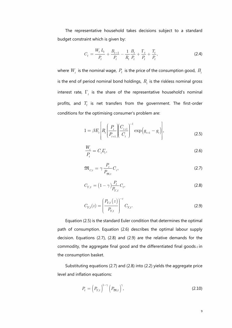
The representative household takes decisions subject to a standard

budget constraint which is given by:

1 1,

t t t t t tt

t t t t t t

W L B B TC

P P R P P P- G

= + - + + (2.4)

where tW is the nominal wage, tP is the price of the consumption good,

tB

is the end of period nominal bond holdings, tR is the riskless nominal gross

interest rate, t

G is the share of the representative household’s nominal

profits, and tT is net transfers from the government. The first-order

conditions for the optimising consumer's problem are:

( )1

11

1

1 exp ,ttt t t t

t t

CPE R g g

P Cb

-

++

+

é ùæ öæ öê ú÷ ÷ç ç÷ ÷ç ç= -ê ú÷ ÷ç ç÷ ÷ê úç ç÷ ÷è øè øê úë û (2.5)

,vt

t t

t

WC L

P= (2.6)

,,t

C t t

t

PC

Pg=

M,

M (2.7)

( ),,

1 ,tY t t

Y t

PC C

Pg= - (2.8)

( ),

, ,,

( ) .Y t

Y t Y tY t

P zC z C

P

e-æ ö÷ç ÷ç ÷= ç ÷ç ÷ç ÷è ø (2.9)

Equation (2.5) is the standard Euler condition that determines the optimal

path of consumption. Equation (2.6) describes the optimal labour supply

decision. Equations (2.7), (2.8) and (2.9) are the relative demands for the

commodity, the aggregate final good and the differentiated final goodsz in

the consumption basket.

Substituting equations (2.7) and (2.8) into (2.2) yields the aggregate price

level and inflation equations:

( ) ( )1

, , ,t Y t tP P Pg g-

= M (2.10)

10

1, ,

( ) ( )t Y t t

g g-P = P PM

(2.11)

where 1/

t t tP P-P = , , , , 1/Y t Y t Y tP P -P = and , 1,

/t t tP P -P =

M M, M are headline,

core and commodity inflation, respectively.

Similarly, substituting equation (2.9) in equation (2.3) defines the price

level of differentiated final goods:

( )1

11 1

, ,0.

Y t Y tP P z dz

ee --é ù= ê ú

ê úë ûò (2.12)

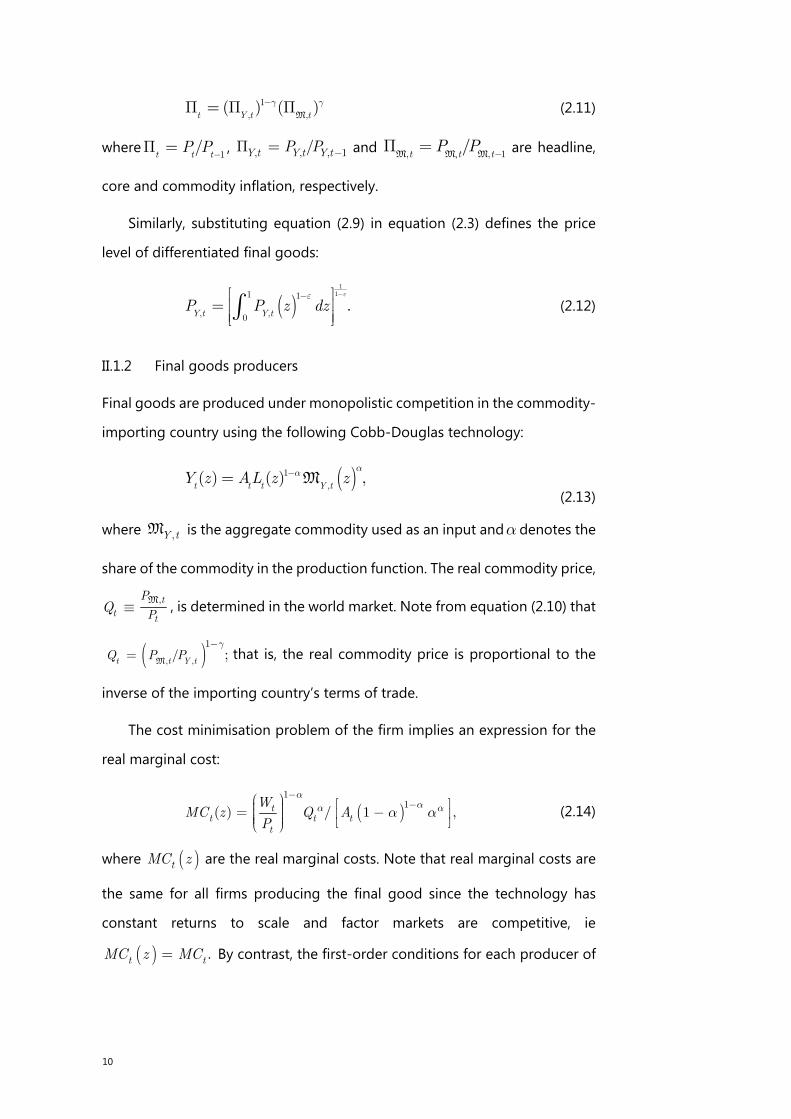
II.1.2 Final goods producers

Final goods are produced under monopolistic competition in the commodity-

importing country using the following Cobb-Douglas technology:

( )1,

( ) ( ) ,t t t Y tY z AL z z

aa-= M (2.13)

where ,Y tM is the aggregate commodity used as an input anda denotes the

share of the commodity in the production function. The real commodity price,

,t

tt

P

PQ º

M , is determined in the world market. Note from equation (2.10) that

( ), ,

1/ ;t t Y tQ P P

g-=

Mthat is, the real commodity price is proportional to the

inverse of the importing country’s terms of trade.

The cost minimisation problem of the firm implies an expression for the

real marginal cost:

( )1

1( ) / 1 ,tt t t

t

WMC z Q A

P

aaa aa a

--æ ö é ù÷ç ÷= -ç ê ú÷ç ÷ç ë ûè ø

(2.14)

where ( )tMC z are the real marginal costs. Note that real marginal costs are

the same for all firms producing the final good since the technology has

constant returns to scale and factor markets are competitive, ie

( ) .t tMC z MC= By contrast, the first-order conditions for each producer of

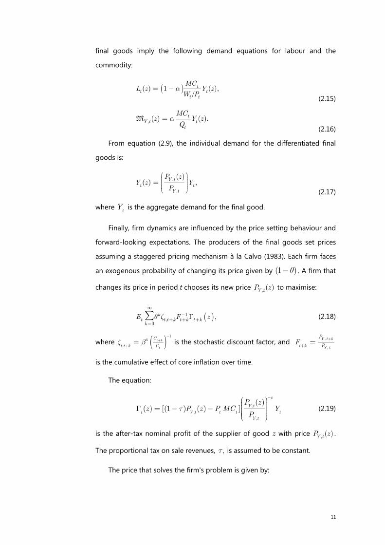
11

final goods imply the following demand equations for labour and the

commodity:

( )( ) 1 ( ),/t

t tt t

MCL z Y z

W Pa= -

(2.15)

, ( ) ( ).tY t t

t

MCz Y z

Qa=M

(2.16)

From equation (2.9), the individual demand for the differentiated final

goods is:

,

,

( )( ) ,Y tt t

Y t

P zY z Y

P

æ ö÷ç ÷ç= ÷ç ÷÷çè ø (2.17)

where tY is the aggregate demand for the final good.

Finally, firm dynamics are influenced by the price setting behaviour and

forward-looking expectations. The producers of the final goods set prices

assuming a staggered pricing mechanism à la Calvo (1983). Each firm faces

an exogenous probability of changing its price given by (1 )q- . A firm that

changes its price in period t chooses its new price , ( )Y tP z to maximise:

( )1,

0,k

t t t k t k t kk

E F zq z¥

-+ + +

=Gå (2.18)

where ( )1

,

t k

t

k

t t k

C

Cz b +

-

+= is the stochastic discount factor, and ,

,

Y t k

Y tt k

P

PF

+

+=

is the cumulative effect of core inflation over time.

The equation:

,,

,

( )( ) [(1 ) ( ) ] Y t

t Y t t t tY t

P zz P z P MC Y

P

e

t

-æ ö÷ç ÷çG = - - ÷ç ÷ç ÷çè ø (2.19)

is the after-tax nominal profit of the supplier of good z with price , ( )Y tP z .

The proportional tax on sale revenues, ,t is assumed to be constant.

The price that solves the firm's problem is given by:

12

, ,0,

,1

,0

( ),

ˆk

t t t k t t k t k t kkY t

Y tk

t t t k t k t kk

E MC Fz

PE F Y

PYe

e

m q z

q z

¥

+ + + +=

¥-

+ + +=

é ùê úê úæ ö ê ú÷ç ê ú÷ ë ûç ÷ =ç ÷ç ÷ é ùç ÷çè ø ê ú

ê úê úê úë û

å

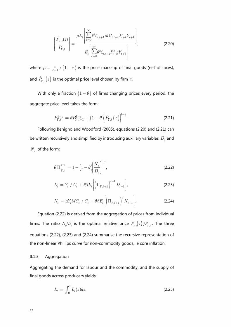
å (2.20)

where ( )1/ 1e

em t

-º - is the price mark-up of final goods (net of taxes),

and ( ),ˆY tP z is the optimal price level chosen by firm z .

With only a fraction ( )1 q- of firms changing prices every period, the

aggregate price level takes the form:

( ) ( )1

1 1, , 1 ,1 ˆ .Y t Y t Y tPP P z

ee eq q

-- -

-é ùê úë û

= + - (2.21)

Following Benigno and Woodford (2005), equations (2.20) and (2.21) can

be written recursively and simplified by introducing auxiliary variables tD and

tN of the form:

( )1

1

,1 1 ,t

tY t

N

D

ee

q q-

- æ ö÷ç ÷çP = - - ÷ç ÷÷çè ø (2.22)

( )1

, 1 1/ ,t t t t Y t tD Y C E De

qb-

+ +

é ùê ú= + Pê úë û

(2.23)

( ), 1 1/ .t t t t t Y t tN YMC C E Ne

m qb + +

é ùê ú= + Pê úë û

(2.24)

Equation (2.22) is derived from the aggregation of prices from individual

firms. The ratio /t tN D is the optimal relative price ( ), ,

/ˆY t Y tz PP . The three

equations (2.22), (2.23) and (2.24) summarise the recursive representation of

the non-linear Phillips curve for non-commodity goods, ie core inflation.

II.1.3 Aggregation

Aggregating the demand for labour and the commodity, and the supply of

final goods across producers yields:

1

0( ) ,t tL L z dz= ò (2.25)

13

,

1

,0( ) ,Y t Y t z dz= òM M (2.26)

111

0.( )t tY Y z dz

eee

e--é ù

ê úê úë û

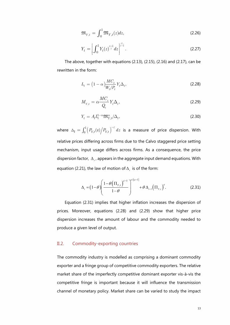
= ò (2.27)

The above, together with equations (2.13), (2.15), (2.16) and (2.17), can be

rewritten in the form:

( )1 ,/t

t t tt t

MCL Y

W Pa= - D (2.28)

,,t

Y t t ttQ

MCM Ya= D (2.29)

1, / ,t t t Y t tY AL a a-= DM (2.30)

where ( )1, ,0(z)Y t Y tt P P dz

e-D = ò is a measure of price dispersion. With

relative prices differing across firms due to the Calvo staggered price setting

mechanism, input usage differs across firms. As a consequence, the price

dispersion factor, t , appears in the aggregate input demand equations. With

equation (2.21), the law of motion of t is of the form:

1 ,

/ 11,1

11

.t t Y tY t

(2.31)

Equation (2.31) implies that higher inflation increases the dispersion of

prices. Moreover, equations (2.28) and (2.29) show that higher price

dispersion increases the amount of labour and the commodity needed to

produce a given level of output.

II.2. Commodity-exporting countries

The commodity industry is modelled as comprising a dominant commodity

exporter and a fringe group of competitive commodity exporters. The relative

market share of the imperfectly competitive dominant exporter vis-à-vis the

competitive fringe is important because it will influence the transmission

channel of monetary policy. Market share can be varied to study the impact

14

of the degree of competitive. That is, the market share of the dominant

commodity exporter can range from zero to one, which corresponds to a

range of market dynamics from perfect competition to a monopoly situation.

II.2.1 Dominant commodity exporter

The dominant exporting country produces the commodity according to the

technology:

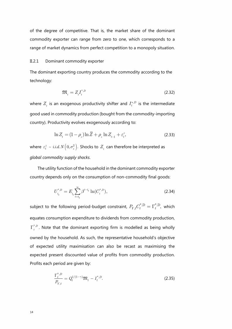
*,Dt t tZ I=M (2.32)

where tZ is an exogenous productivity shifter and ,D

tI* is the intermediate

good used in commodity production (bought from the commodity-importing

country). Productivity evolves exogenously according to:

1ln (1 )ln ln ,z

t z z t tZ Z Zr r e-= - + + (2.33)

where ( )2~ . . . 0, .zt zi i d Ne s Shocks to

tZ can therefore be interpreted as

global commodity supply shocks.

The utility function of the household in the dominant commodity exporter

country depends only on the consumption of non-commodity final goods:

0

0 0

0

*, *,ln( ),t tD Dt t t

t t

U E Cb¥

-

=

= å (2.34)

subject to the following period-budget constraint, *,D *,D, ,Y t t tP C = G which

equates consumption expenditure to dividends from commodity production,

*,Dt

G . Note that the dominant exporting firm is modelled as being wholly

owned by the household. As such, the representative household’s objective

of expected utility maximisation can also be recast as maximising the

expected present discounted value of profits from commodity production.

Profits each period are given by:

*,1/(1 ) *,

,

.D

Dtt t t

Y t

Q IP

g-G= -M (2.35)

15

The consumption good, *,D

tC , and the intermediate good, , ,DtI

* are

demanded by the commodity-exporting countries. The dominant commodity

exporter chooses the level of commodity output, tM , such that it maximises

the expected present discounted utility of the representative household in

equation (2.34), subject to demand from the commodity-importing country

and supply from the competitive fringe of commodity exporters.9

II.2.2 Fringe of competitive commodity exporters

Similarly, the utility function of households in the fringe depends only on the

consumption of final goods:

( )*, *,lno

ooo

t tF Ft ttt t

U E Cb¥

-

== å , (2.36)

subject to the following period-budget constraint, *, *,

,,F F

Y t t tP C = G which

equates consumption expenditure to dividends from commodity production,

*,.F

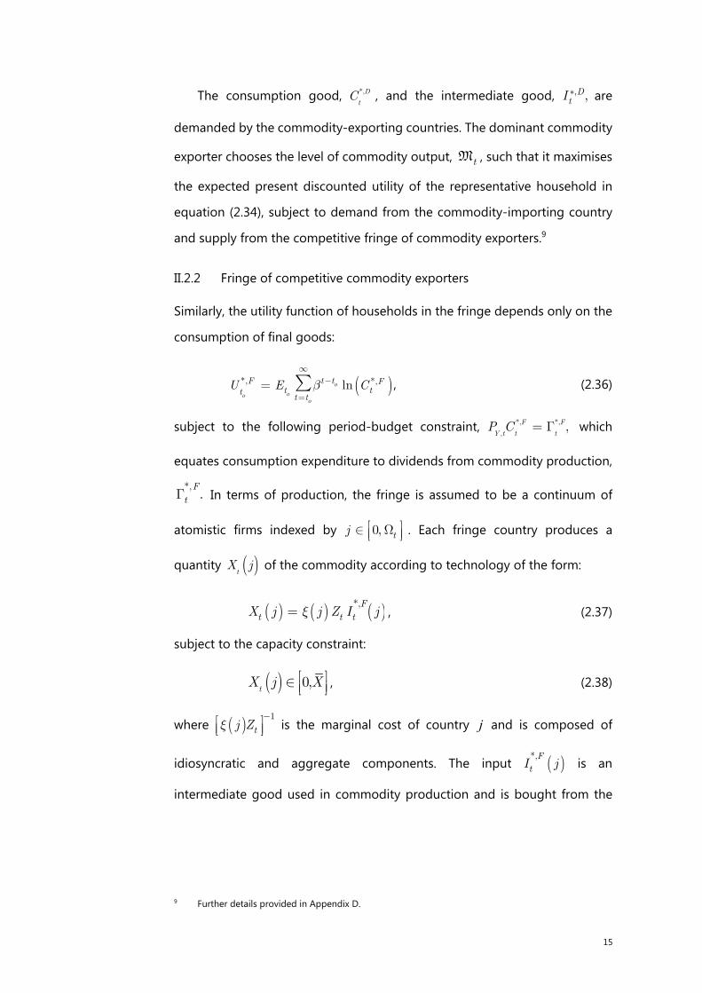
tG In terms of production, the fringe is assumed to be a continuum of

atomistic firms indexed by 0, tj é ùÎ Wê úë û . Each fringe country produces a

quantity ( )tX j of the commodity according to technology of the form:

( ) ( ) ( )*,t t t

FX j j Z I jx= , (2.37)

subject to the capacity constraint:

( ) 0,tX j Xé ùÎ ê úë û , (2.38)

where ( )1

tj Zx-é ù

ê úë û is the marginal cost of country j and is composed of

idiosyncratic and aggregate components. The input ( )*,FtI j is an

intermediate good used in commodity production and is bought from the

9 Further details provided in Appendix D.

16

commodity-importing country (ie the final goods produced in the

commodity-importing country).

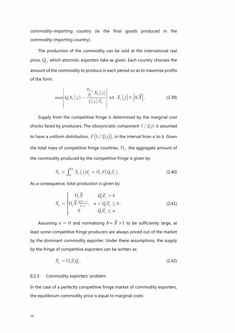
The production of the commodity can be sold at the international real

price, ,tQ which atomistic exporters take as given. Each country chooses the

amount of the commodity to produce in each period so as to maximise profits

of the form:

( )( )

( )

,

max

Y t

tt

t tt

P

P X jX j

ZQ

jx

é ùê úê ú-ê úê úê úë û

s.t. ( ) 0,tX j Xé ùÎ ê úë û . (2.39)

Supply from the competitive fringe is determined by the marginal cost

shocks faced by producers. The idiosyncratic component 1 / ( )jx is assumed

to have a uniform distribution, ( )1/ ( )F jx , in the interval from a to b. Given

the total mass of competitive fringe countries, ,t

W the aggregate amount of

the commodity produced by the competitive fringe is given by:

( ) ( )0

t

t t j t t tX X j d F Q ZW

º = Wò . (2.40)

As a consequence, total production is given by:

,

0

t t

t t tQ Z a

t t t tb a

t t

X Q Z b

X X a Q Z b

Q Z a

-

-

ìï W >ïïïï= W < £íïî

£ïïïï

. (2.41)

Assuming 0a = and normalising 1b X to be sufficiently large, at

least some competitive fringe producers are always priced out of the market

by the dominant commodity exporter. Under these assumptions, the supply

by the fringe of competitive exporters can be written as:

t t t tX ZQ=W . (2.42)

II.2.3 Commodity exporters’ problem

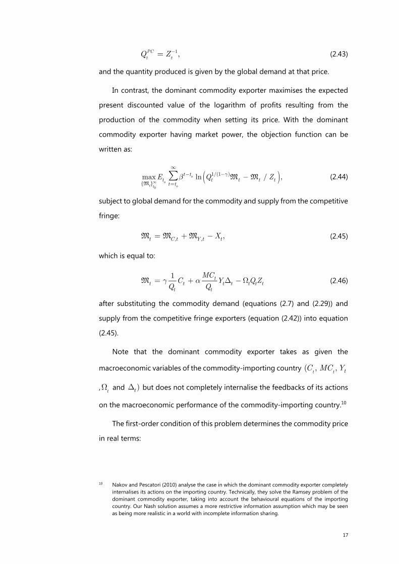
In the case of a perfectly competitive fringe market of commodity exporters,

the equilibrium commodity price is equal to marginal costs:

17

1,PC

t tQ Z-= (2.43)

and the quantity produced is given by the global demand at that price.

In contrast, the dominant commodity exporter maximises the expected

present discounted value of the logarithm of profits resulting from the

production of the commodity when setting its price. With the dominant

commodity exporter having market power, the objection function can be

written as:

( )0

1/(1 )

}max ln / ,o

ot t o

t tt t t t tt t

E Q Zgb¥

¥--

=-å

{MM M (2.44)

subject to global demand for the commodity and supply from the competitive

fringe:

, , ,t C t Y t tX= + -M M M (2.45)

which is equal to:

1 tt t t t t t t

t t

MCC Y Q Z

Q Qg a= + D -WM (2.46)

after substituting the commodity demand (equations (2.7) and (2.29)) and

supply from the competitive fringe exporters (equation (2.42)) into equation

(2.45).

Note that the dominant commodity exporter takes as given the

macroeconomic variables of the commodity-importing country ( ,tC ,

tMC tY

,t

W and )tD but does not completely internalise the feedbacks of its actions

on the macroeconomic performance of the commodity-importing country.10

The first-order condition of this problem determines the commodity price

in real terms:

10 Nakov and Pescatori (2010) analyse the case in which the dominant commodity exporter completely

internalises its actions on the importing country. Technically, they solve the Ramsey problem of the dominant commodity exporter, taking into account the behavioural equations of the importing country. Our Nash solution assumes a more restrictive information assumption which may be seen as being more realistic in a world with incomplete information sharing.

18

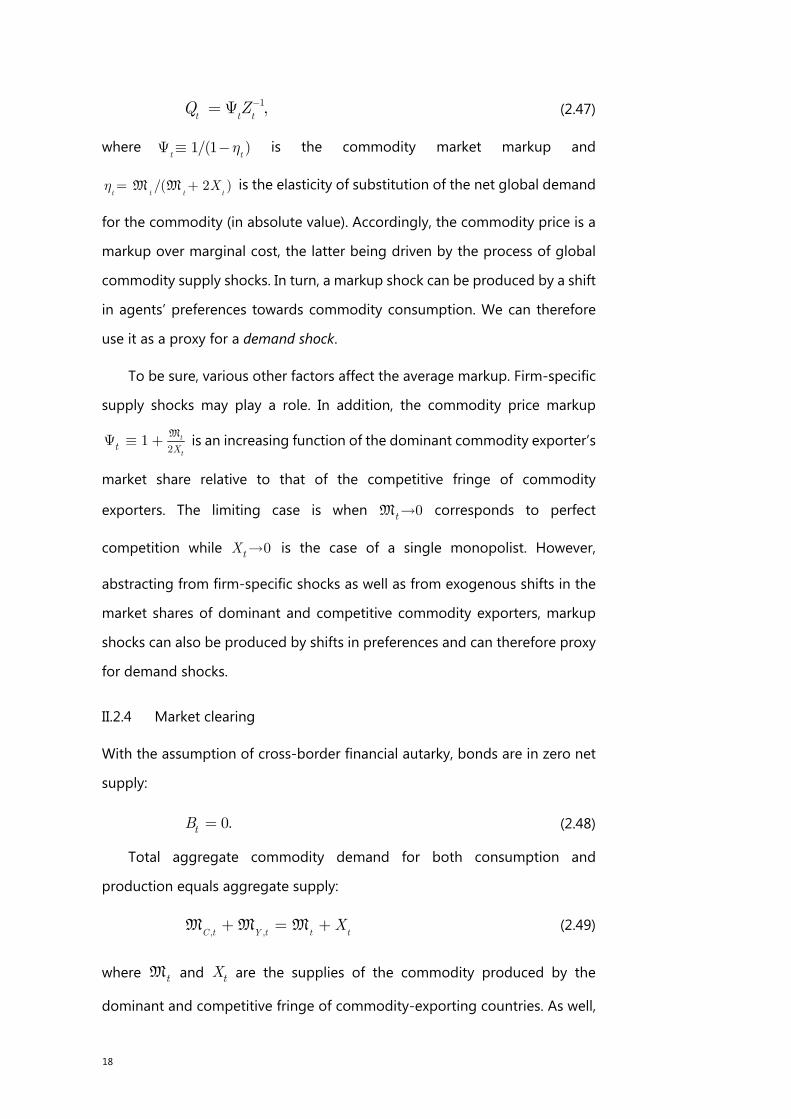
1,t t tQ Z-= Y (2.47)

where 1/(1 )t t

hY º - is the commodity market markup and

/( 2 )t t t t

Xh = +M M is the elasticity of substitution of the net global demand

for the commodity (in absolute value). Accordingly, the commodity price is a

markup over marginal cost, the latter being driven by the process of global

commodity supply shocks. In turn, a markup shock can be produced by a shift

in agents’ preferences towards commodity consumption. We can therefore

use it as a proxy for a demand shock.

To be sure, various other factors affect the average markup. Firm-specific

supply shocks may play a role. In addition, the commodity price markup

21 t

tt X

Y º + M is an increasing function of the dominant commodity exporter’s

market share relative to that of the competitive fringe of commodity

exporters. The limiting case is when 0tM corresponds to perfect

competition while 0tX is the case of a single monopolist. However,

abstracting from firm-specific shocks as well as from exogenous shifts in the

market shares of dominant and competitive commodity exporters, markup

shocks can also be produced by shifts in preferences and can therefore proxy

for demand shocks.

II.2.4 Market clearing

With the assumption of cross-border financial autarky, bonds are in zero net

supply:

0.tB = (2.48)

Total aggregate commodity demand for both consumption and

production equals aggregate supply:

, ,C t Y t t tX+ = +M M M (2.49)

where tM and tX are the supplies of the commodity produced by the

dominant and competitive fringe of commodity-exporting countries. As well,

19

labour supply is set equal to labour demand in the commodity-importing

economy.

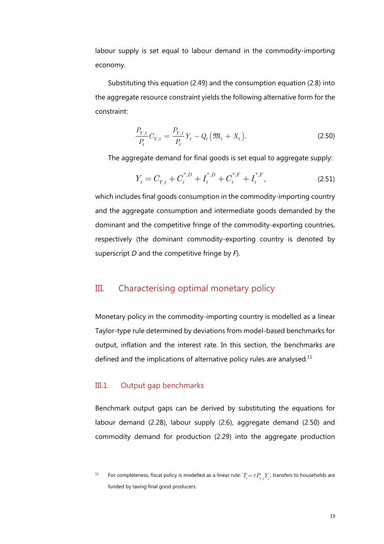
Substituting this equation (2.49) and the consumption equation (2.8) into

the aggregate resource constraint yields the following alternative form for the

constraint:

( ), ,, .Y t Y tY t t t t t

t t

P PC Y Q X

P P= - +M (2.50)

The aggregate demand for final goods is set equal to aggregate supply:

*, *, *, *,

,

D D

t Y t t t t

F F

tY C C I C I= + + + + , (2.51)

which includes final goods consumption in the commodity-importing country

and the aggregate consumption and intermediate goods demanded by the

dominant and the competitive fringe of the commodity-exporting countries,

respectively (the dominant commodity-exporting country is denoted by

superscript D and the competitive fringe by F).

III. Characterising optimal monetary policy

Monetary policy in the commodity-importing country is modelled as a linear

Taylor-type rule determined by deviations from model-based benchmarks for

output, inflation and the interest rate. In this section, the benchmarks are

defined and the implications of alternative policy rules are analysed.11

III.1. Output gap benchmarks

Benchmark output gaps can be derived by substituting the equations for

labour demand (2.28), labour supply (2.6), aggregate demand (2.50) and

commodity demand for production (2.29) into the aggregate production

11 For completeness, fiscal policy is modelled as a linear rule: ,t Y t t

T P Yt= ; transfers to households are

funded by taxing final good producers.

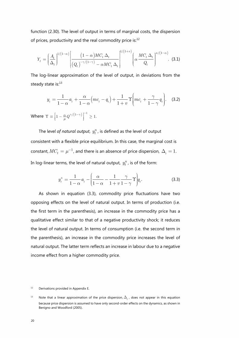
20

function (2.30). The level of output in terms of marginal costs, the dispersion

of prices, productivity and the real commodity price is:12

( ) ( )

( ) ( )

( ) ( )1/ 1 / 11/ 1

/ 1.

1v

t t t ttt

t tt t t

MC MCAY

QQ MC

a aa

g g

aa

a

+ --

- -

é ù æ ö- D Dæ ö ê ú ÷ç÷ç ÷ç÷ ê ú= ç ÷ç÷ ÷ç ÷ç ê ú çD ÷çè ø è ø- Dê úë û

(3.1)

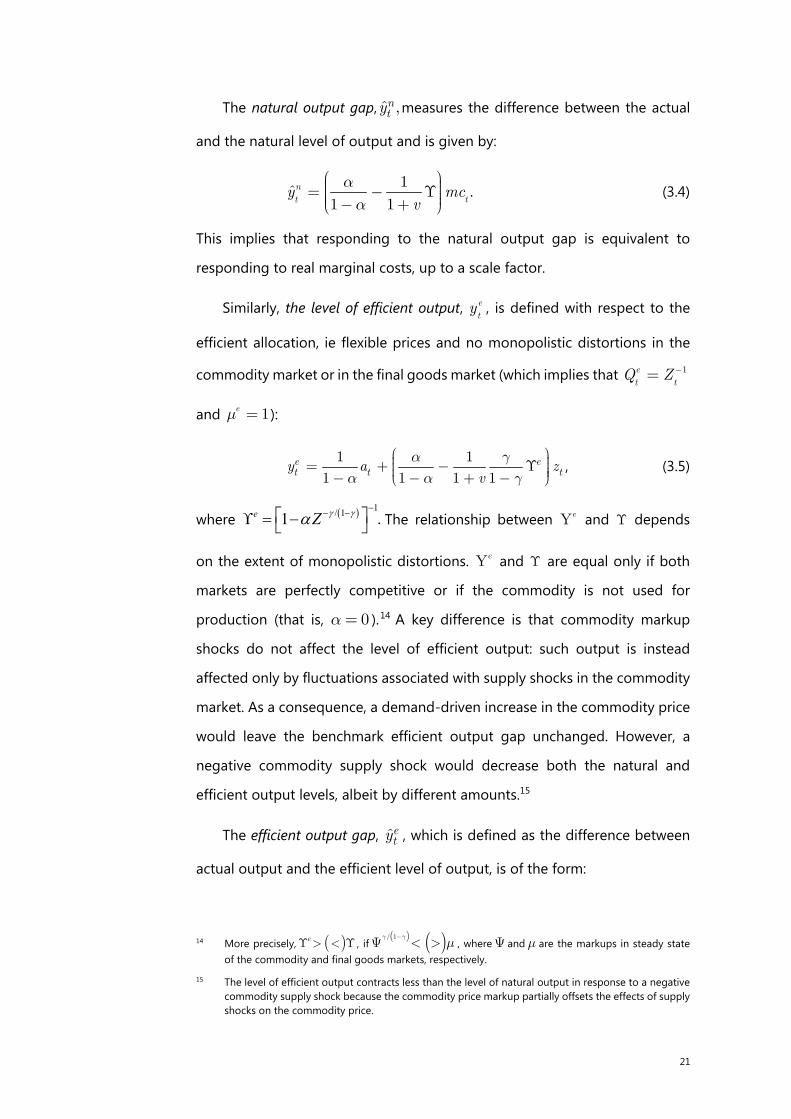
The log-linear approximation of the level of output, in deviations from the

steady state is:13

( )1 11 1 1 1t t t t t t

y a mc q mc qv

a ga a g

æ ö÷ç ÷= + - + ¡ +ç ÷ç ÷ç- - + -è ø. (3.2)

Where ( ) 1/ 11 1.Qg ga

m

--¡ º - ³é ùê úë û

The level of natural output, nty , is defined as the level of output

consistent with a flexible price equilibrium. In this case, the marginal cost is

constant, 1tMC m-= , and there is an absence of price dispersion, 1.

tD =

In log-linear terms, the level of natural output, nty , is of the form:

1 11

.1 1 1

nt t ty a q

v

a ga a g

æ ö÷ç ÷= - - ¡ç ÷ç ÷ç- - + -è ø (3.3)

As shown in equation (3.3), commodity price fluctuations have two

opposing effects on the level of natural output. In terms of production (i.e.

the first term in the parenthesis), an increase in the commodity price has a

qualitative effect similar to that of a negative productivity shock; it reduces

the level of natural output. In terms of consumption (i.e. the second term in

the parenthesis), an increase in the commodity price increases the level of

natural output. The latter term reflects an increase in labour due to a negative

income effect from a higher commodity price.

12 Derivations provided in Appendix E.

13 Note that a linear approximation of the price dispersion, tD , does not appear in this equation

because price dispersion is assumed to have only second-order effects on the dynamics, as shown in Benigno and Woodford (2005).

21

The natural output gap, ˆ ,nty measures the difference between the actual

and the natural level of output and is given by:

11 1

ˆ .t

nt

mcv

yaa

æ ö÷ç ÷= - ¡ç ÷ç ÷ç - +è ø (3.4)

This implies that responding to the natural output gap is equivalent to

responding to real marginal costs, up to a scale factor.

Similarly, the level of efficient output, e

ty , is defined with respect to the

efficient allocation, ie flexible prices and no monopolistic distortions in the

commodity market or in the final goods market (which implies that 1e

t tQ Z-=

and 1em = ):

1 11 1 1 1

e et t ty a z

v

a ga a g

æ ö÷ç= + - ¡ ÷ç ÷ç ÷è ø- - + -, (3.5)

where / 1 11 .e Z The relationship between eU and ¡ depends

on the extent of monopolistic distortions. eU and ¡ are equal only if both

markets are perfectly competitive or if the commodity is not used for

production (that is, 0a= ).14 A key difference is that commodity markup

shocks do not affect the level of efficient output: such output is instead

affected only by fluctuations associated with supply shocks in the commodity

market. As a consequence, a demand-driven increase in the commodity price

would leave the benchmark efficient output gap unchanged. However, a

negative commodity supply shock would decrease both the natural and

efficient output levels, albeit by different amounts.15

The efficient output gap, ety , which is defined as the difference between

actual output and the efficient level of output, is of the form:

14 More precisely, ( )e¡ > < ¡ , if

( ) ( )/ 1g g m-Y < > , where Y andm are the markups in steady state

of the commodity and final goods markets, respectively.

15 The level of efficient output contracts less than the level of natural output in response to a negative commodity supply shock because the commodity price markup partially offsets the effects of supply shocks on the commodity price.

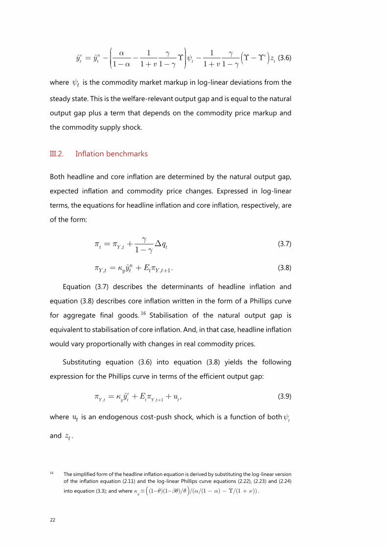
22

( )1 1ˆ ˆ

1 1 1 1 1e n et t t ty y z

v v

a g gy

a g g

æ ö÷ç ÷= - - ¡ - ¡-¡ç ÷ç ÷ç - + - + -è ø (3.6)

where ty is the commodity market markup in log-linear deviations from the

steady state. This is the welfare-relevant output gap and is equal to the natural

output gap plus a term that depends on the commodity price markup and

the commodity supply shock.

III.2. Inflation benchmarks

Both headline and core inflation are determined by the natural output gap,

expected inflation and commodity price changes. Expressed in log-linear

terms, the equations for headline inflation and core inflation, respectively, are

of the form:

, 1t Y t tqgp pg

= + D-

(3.7)

, , 1n

Y t y t t Y ty Ep k p += + . (3.8)

Equation (3.7) describes the determinants of headline inflation and

equation (3.8) describes core inflation written in the form of a Phillips curve

for aggregate final goods. 16 Stabilisation of the natural output gap is

equivalent to stabilisation of core inflation. And, in that case, headline inflation

would vary proportionally with changes in real commodity prices.

Substituting equation (3.6) into equation (3.8) yields the following

expression for the Phillips curve in terms of the efficient output gap:

, , 1ˆe

Y t y t t Y t ty E up k p

+= + + , (3.9)

where tu is an endogenous cost-push shock, which is a function of botht

y

and tz .

16 The simplified form of the headline inflation equation is derived by substituting the log-linear version

of the inflation equation (2.11) and the log-linear Phillips curve equations (2.22), (2.23) and (2.24)

into equation (3.3); and where ( )(1 )(1 )/ /( /(1 ) /(1 ))y

k q bq q a a nº - - - - ¡ + .

23

In this model, the divine coincidence featured in models with exogenous

commodity prices is broken. It is no longer possible to simultaneously

stabilise core inflation and the welfare-relevant output gap. The trade-off

arises from the impact of commodity price fluctuations on the level of efficient

output. An increase in commodity price markups generates a positive cost-

push shock, which puts upward pressure on core inflation but lowers the

efficient output gap.

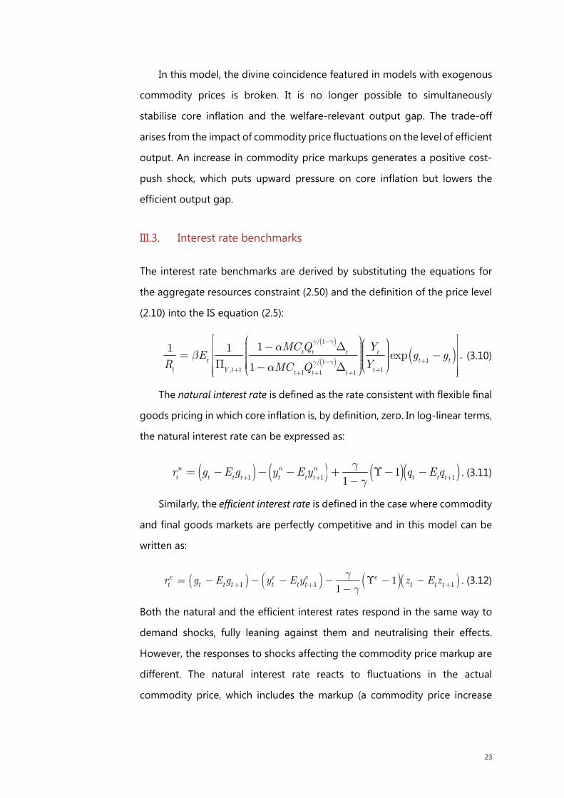
III.3. Interest rate benchmarks

The interest rate benchmarks are derived by substituting the equations for

the aggregate resources constraint (2.50) and the definition of the price level

(2.10) into the IS equation (2.5):

( )

( ) ( )/ 1

1/ 1, 1 11 1 1

11 1exp .

1t t t t

t t t

t Y t tt t t

MCQ YE g g

R YMC Q

g g

g g

ab

a

-

+-+ ++ + +

é ùæ öæ ö÷- Dçê ú÷ç÷ç ÷÷ç= -ê úç ÷÷çç ÷÷ç ÷ê úP ç è ø÷- Dçè øê úë û

(3.10)

The natural interest rate is defined as the rate consistent with flexible final

goods pricing in which core inflation is, by definition, zero. In log-linear terms,

the natural interest rate can be expressed as:

( ) ( ) ( )( )1 1 11

1n n nt t t t t t t t t tr g E g y E y q E q

gg+ + += - - - + ¡- -

-. (3.11)

Similarly, the efficient interest rate is defined in the case where commodity

and final goods markets are perfectly competitive and in this model can be

written as:

( ) ( ) ( )( )1 1 111

e e e et t t t t t t t t tr g E g y E y z E z

gg+ + += - - - - ¡ - -

-. (3.12)

Both the natural and the efficient interest rates respond in the same way to

demand shocks, fully leaning against them and neutralising their effects.

However, the responses to shocks affecting the commodity price markup are

different. The natural interest rate reacts to fluctuations in the actual

commodity price, which includes the markup (a commodity price increase

24

driven by a higher markup boosts the natural interest rate), while the efficient

interest rate does not respond to changes in the markup.

III.4. Analysing monetary policy rules

This section explores the model dynamics under alternative monetary policy

rules, highlighting the differential responses to demand and commodity

supply shocks. The baseline policy rule assumes that the monetary authority

responds to core inflation and the efficient output gap.17 It is of the form:

| 1 , +ˆ cot t m te e

t t core Y t y t qr E r y jj p j-é ù Dê úë û

= + + , (3.13)

where the relative weights on core inflation and the output gap determine

the trade-off between core inflation and output gap stabilisation. The

benchmark interest rate also influences the optimal policy setting. We

additionally assume that the monetary authority is able to observe inflation

and output with a one period lag – hence the presence of the expectations

operator – whereas commodity prices are available in real time. Therefore, the

central bank uses the forecast (ie the expectation based on the information

set available in the previous period) of inflation and output to conduct

monetary policy and the observed (contemporaneous) change in the

commodity price ∆q.

The size of the shocks are standardised to generate a 1% increase in the

commodity price under a benchmark scenario; the coefficients of the policy

rule have been calibrated to result in 1.5corej = , 0.5yj = and 0.05.comj =

For most structural parameters, the calibration is in line with those found in

the literature (Table 1). For the parameters associated with the commodity

market, the choice is a bit more arbitrary owing to the less conventional view

of the literature. The share of the commodity in the consumption basket is set

to 10%, which roughly matches the share of primary commodity inputs in the

17 Of course, similar results could be obtained for the natural benchmark. We focus here on the efficient

benchmark as it is the one that actually matters for welfare calculations. We will explore alternative and easier-to-compute benchmarks in what follows.

25

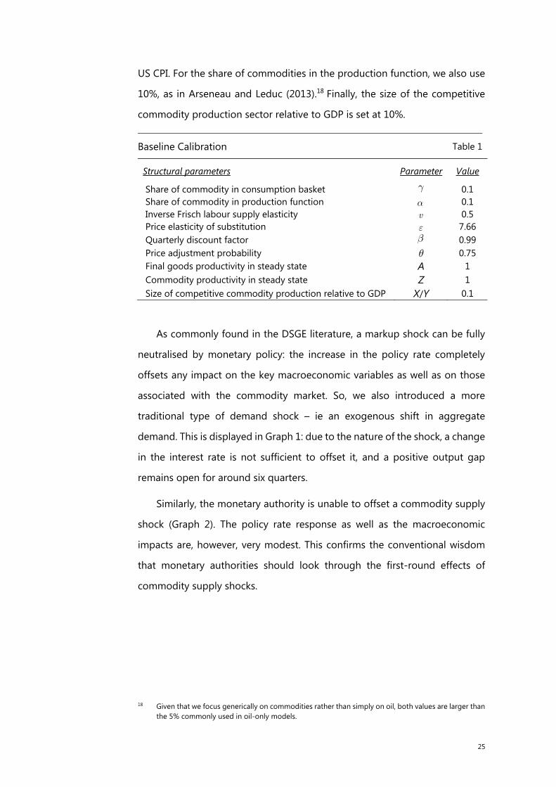
US CPI. For the share of commodities in the production function, we also use

10%, as in Arseneau and Leduc (2013).18 Finally, the size of the competitive

commodity production sector relative to GDP is set at 10%.

Baseline Calibration Table 1

Structural parameters Parameter Value

Share of commodity in consumption basket g 0.1 Share of commodity in production function a 0.1 Inverse Frisch labour supply elasticity v 0.5 Price elasticity of substitution e 7.66 Quarterly discount factor b 0.99 Price adjustment probability q 0.75 Final goods productivity in steady state A 1 Commodity productivity in steady state Z 1 Size of competitive commodity production relative to GDP X/Y 0.1

As commonly found in the DSGE literature, a markup shock can be fully

neutralised by monetary policy: the increase in the policy rate completely

offsets any impact on the key macroeconomic variables as well as on those

associated with the commodity market. So, we also introduced a more

traditional type of demand shock – ie an exogenous shift in aggregate

demand. This is displayed in Graph 1: due to the nature of the shock, a change

in the interest rate is not sufficient to offset it, and a positive output gap

remains open for around six quarters.

Similarly, the monetary authority is unable to offset a commodity supply

shock (Graph 2). The policy rate response as well as the macroeconomic

impacts are, however, very modest. This confirms the conventional wisdom

that monetary authorities should look through the first-round effects of

commodity supply shocks.

18 Given that we focus generically on commodities rather than simply on oil, both values are larger than

the 5% commonly used in oil-only models.

26

III.4.1 A note on the natural benchmark

To simplify the discussion, we do not report the impulse responses for the

natural policy rule. It is useful to note, however, that the dynamics associated

with a commodity supply shock generate similarities and differences

compared to the efficient rule. For both the natural and efficient benchmarks,

a negative supply shock increases the commodity’s price, boosts headline

inflation and reduces the amount of the commodity supplied by the

exporters. The levels of natural and efficient output both decline, with the

level of efficient output falling more. In the efficient case, the decline in the

level of efficient output partially offsets the increase in the commodity’s price

via a reduction in the markup. The trade-off between inflation and output are

different in the two cases. Core inflation and the output gap are completely

stabilised in the natural benchmark case. But in the efficient benchmark case,

the efficient output gap rises and core inflation declines. This indicates that a

monetary authority following an efficient policy rule partially offsets the

effects of the higher commodity price on headline inflation with lower core

inflation.

III.4.2 Welfare calculations

The performance of the efficient policy rule in equation (3.13) is also assessed

in terms of the welfare of the representative household (ie from the

commodity-importing country), along with two alternative policy rules that

take the general form:

| 1 , t te

t t core Y tr E r j p-é ùê úë û

= + (3.14)

And:

| 1 t t te

t t headr E r j p-é ùê úë û= + (3.15)

27

For policy rule (3.14), the monetary authority responds only to core

inflation. For policy rule (3.15), the response is to headline instead of core

inflation.19

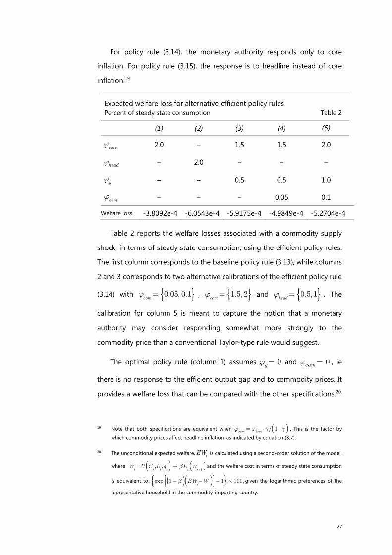
Expected welfare loss for alternative efficient policy rules Percent of steady state consumption Table 2

(1) (2) (3) (4) (5)

core

j 2.0 – 1.5 1.5 2.0

headj – 2.0 – – –

y

j – – 0.5 0.5 1.0

com

j – – – 0.05 0.1

Welfare loss -3.8092e-4 -6.0543e-4 -5.9175e-4 -4.9849e-4 -5.2704e-4

Table 2 reports the welfare losses associated with a commodity supply

shock, in terms of steady state consumption, using the efficient policy rules.

The first column corresponds to the baseline policy rule (3.13), while columns

2 and 3 corresponds to two alternative calibrations of the efficient policy rule

(3.14) with { }0.05, 0.1com

j = , { }1.5, 2core

j = and { }0.5, 1head

j = . The

calibration for column 5 is meant to capture the notion that a monetary

authority may consider responding somewhat more strongly to the

commodity price than a conventional Taylor-type rule would suggest.

The optimal policy rule (column 1) assumes 0yj = and 0comj = , ie

there is no response to the efficient output gap and to commodity prices. It

provides a welfare loss that can be compared with the other specifications.20,

19 Note that both specifications are equivalent when ( )/ 1com core

j j g g⋅= - . This is the factor by

which commodity prices affect headline inflation, as indicated by equation (3.7).

20 The unconditional expected welfare, tEW is calculated using a second-order solution of the model,

where ( ) ( )1

, ,t t t t t tW U C L g E Wb

+= + and the welfare cost in terms of steady state consumption

is equivalent to ( )( ){ }exp 1 1 100,t

EW Wb- - - ´é ùê úë û given the logarithmic preferences of the

representative household in the commodity-importing country.

28

21 In columns 2, 3, 4 and 5, the policy rules that respond directly to the

commodity’s price and headline inflation generate larger welfare losses than

the policy rule in column 1. This is because the policy rule of column 1 already

takes into account the effects of the commodity’s price; the additional

responses to changes in the commodity price and headline inflation in the

alternative policy rules simply generate more volatile interest rates than is

optimal. These results highlight the importance of monitoring and responding

to core inflation rather than headline inflation. Note, however, that a

moderate response to commodity prices (column 4) reduces welfare losses

compared to the optimal policy (3.14).

IV. Incomplete information, misdiagnosis and monetary

policy spillovers

In practice, monetary authorities do not know in real time which shocks are

affecting their jurisdictions: all they can observe are movements in the

international prices of commodities. Moreover, the readings on inflation and

output will not be available in real time. Given that the optimal responses to

demand and supply shocks differ, this complicates the formulation of an

appropriate monetary policy reaction,. On top of this, a supply shock would

affect the efficient output benchmark, while a demand shock would not, which

would generate additional uncertainty on the output gap.

This section considers the challenges arising from misdiagnosis, ie the risk

that a monetary authority misinterprets the source of the shocks driving

commodity price fluctuations. The optimal monetary policy response to

demand and supply shocks differs: the optimal response to demand shocks

is to fully neutralise their effects on output and inflation, so that the

21 The results corresponding to preference shocks are the same under all of the policy rules, and thus are not reported. Also, this policy rule offers positive, albeit small, welfare gains in comparison to the natural policy rule alternative (in which core inflation and the output gap are perfectly stabilised as in Graph 1).

29

commodity’s price is stabilised. By contrast, the optimal response to negative

commodity supply shocks is to partially offset their effects on headline

inflation by a reduction in both core inflation and the output gap. As a

consequence, misdiagnosis of the source of the shocks will lead to a

deterioration in economic outcomes.

IV.1. Monetary policy under incomplete information

As pointed out in Section III, the source of the shocks matters for the

determination of the benchmark output gap and natural rate. This

complicates the real-time problem that policymakers face, ie the inability to

observe output and inflation in real time. In practice, policymakers observe

commodity prices in a timely fashion but only observe output and inflation

with a lag. So there is the risk that a monetary authority will misdiagnose the

state of the economy in real time. In this section, we highlight the monetary

policy challenges under two types of learning: the first is a classical signal

extraction problem in which the monetary authority bases its assessment of

commodity demand and supply shocks on past data; and the second in which

the monetary authority updates its assessments of the source of the shocks

with information about how the economy responds to its monetary policy

actions.

IV.2. The signal-extraction problem

In the previous section, the degree of uncertainty faced by the monetary

authority is limited to shocks to the benchmarks. In this section, we consider

the decision-making problem faced by the monetary authority when it does

not observe the supply and demand shocks ( tz and t

y ) driving the

commodity’s price. The monetary authority can only infer the shocks from

past behaviour. To model this, we assume the commodity price takes the

form:

t t t tq z Hy x¢=- + = , (4.1)

30

where 1 1H é ù¢ = -ê úë û and [ ]t t tzx y ¢= . The unconditional variance of

tx is:

2

2var( ) z z

tz

P y

y y

s sx

s s

é ùê úº = ê úê úë û

. (4.2)

Given this informational structure, the monetary authority infers the sources

of commodity price fluctuations by solving a signal-extraction problem using

a Kalman filter, ie:

t tma

t tE z Mqy

¢é ù =ê úë û, (4.3)

where 1[ ' ]M PH H PH -= is a weighted average of the variances and

covariances of tz and t

y ; M is calculated as:

12 2 1 x

xxM

x x

rrr

é ù-ê ú= ê ú-- + ê úë û, (4.4)

where ( , )t tcorr zr y= and /z

x ys s= .22

Three cases of equation (4.3) help to shed light on the trade-offs facing

the monetary authority. In the first case (type A), when 0x , the volatility

of the commodity supply shock is high relative to that of the commodity

market markup. In this case, the monetary authority attributes nearly all of the

fluctuations to the commodity price markup. That is:

if 0, .0t tma

ttx E z qy ¢ ¢é ù é ù ê ú ê úë û ë û

In the case (type B), all the commodity price fluctuations are attributed to

the supply shock. That is:

if , 0 .mt t ta

tx E z qy ¢ ¢é ù é ù¥ -ê ú ê úë û ë û

In the last case (type C), the monetary authority attributes commodity

price fluctuations partially to each component of the commodity price, taking

into account the relative volatility and correlation the components, as in

22 See chapter 13 of Hamilton (1994) for the derivation.

31

equation (4.4). Given the monetary authority’s inference of the drivers of

commodity price fluctuations, ( )t tmaE z and ( )t t

maE y , the monetary authority

uses the policy benchmarks, ( )stma s

tE r and ( )ˆt

ma ss

tE y , in the policy rule (3.13).

IV.3. Implications for the monetary policy model in Section III

We start with the monetary authority’s policy rule in Section III:

| 1 , +ˆ cot t m te e

t t core Y t y t qr E r y jj p j-é ù Dê úë û

= + + , (4.5)

wherecore

j and yj capture the relative weight of stabilising inflation and the

welfare-relevant output gap. Given ( )t t

maE z and ( )t t

maE y , the monetary

authority can form expectations based on the inferred origin of the shock

driving the change in commodity prices ∆q. If the monetary authority fails to

correctly identify the shocks driving the commodity price fluctuation, a policy

error arises. That is:

,

,

| 1

| 1

ˆ

ˆ ,

e ecom t

e ecom t

t Y t y t

t Y t y t

mat t t

t t t

r y

r y

r E

eqE

qp

p

j p j

j p j

j

j-

-

é ù+ +ê úë ûé ù+ +ê úë û

+ D

= ++ D

= (4.6)

where:

( ) ( ) ( ) ( )( ) ( )

| 1 | 1 | 1 , | 1 ,

| 1 | 1ˆ ˆ

e et t t t t t t core t t Y t t t Y t

e ey t t t t

ma ma

mt t

a

e E r E r E E

E y E y

j p p

j- - - -

- -

é ù é ùº - + -ê ú ê úë û ë ûé ù+ -ê úë û

corresponds to a misdiagnosis error, which is an endogenous variable, and

| 1

m

t t

aE-

denotes the expectations under the incorrect diagnosis on the source

of the shock. Note that when the monetary authority imputes the change in

commodity prices to the wrong type of shock, its estimates of endogenous

variables will be incorrect, leading to persistent errors in the interest rate

setting.23 To see this, we augment our dynamic system with equation (4.6) and

analyse the implications for the impulse responses.

23 If the monetary authority correctly identifies the source of the shock, the error is zero.

32

Graph 3 shows the impulse responses to a commodity supply shock in

the misdiagnosis case A. Even though the commodity price is driven by a

supply shock, the monetary authority misdiagnoses it as a traditional

demand-driven commodity shock. If the monetary authority fails to recognise

that an increase in the commodity price is driven by external supply

conditions, the consequence is overly tight monetary policy accompanied by

an excessive drop in both output and inflation. The commodity price rises less

than in the baseline case because of tighter monetary policy. Core and

headline inflation both fall because of the economy’s slowdown.

Graph 4 shows the impulse responses to a conventional aggregate

demand shock in the case of misdiagnosis type B, in which the rise in the

commodity’s price is mistakenly attributed to a negative commodity supply

shock. In this case, the easier monetary policy associated with an attempt to

look-through the rise in the commodity price results in higher output and

inflation. This type of policy misdiagnosis induces a very procyclical increase

in the commodity price.

Graphs 5 and 6 report the results for the case of a misdiagnosis of type

C, in which the monetary authority implements an optimally weighted

response to the commodity price rise based on the historical correlation of

commodity demand and supply shocks as per equation (4.4). The standard

deviations of the supply and demand shocks for the Kalman filter are

calibrated to the empirical estimates by Filardo and Lombardi (2013), which

yields a ratio (x in equation (4.4)) of about 1.5. Consistent with the general

conclusions from misdiagnosis types A and B, the monetary authority

responds excessively to supply shocks and insufficiently to demand shocks:

hence, monetary policy turns out overall to be excessively procyclical.

The results for the different types of diagnosis risk underscore the

modelling and policy implications of this informational restriction. On the

modelling side, the misdiagnosis risk leads to a breakdown of the divine

coincidence found in full information models à la Blanchard and Gali (2007).

33

On the policy implication side, the difference between equations (3.9) and

(4.6) implies a failure to stabilise core inflation in the short run (as is verified

in Graphs 3-6). As a consequence, and to the extent to which the monetary

authority cannot infer the nature of the shocks perfectly, the policy reaction

will inherently tend to amplify fluctuations in commodity prices and the

macroeconomy more generally. In the case where the monetary authority

misinterprets a rise in the commodity price as supply-driven, the contraction

in both output and core inflation would be larger than in the full information

case. And, in the case where commodity price fluctuations are driven by global

demand, the monetary authority would amplify cyclical fluctuations and, as a

result, destabilise the economy. These results underscore the importance of

correctly identifying the underlying nature of commodity price shocks. A

corollary of this is that if monetary authorities can and do take efforts to learn

about the true nature of the shocks, they can improve macroeconomic

outcomes. Finally, the results suggest that a monetary authority focused on

core inflation would help to stabilise the economy more actively in the

presence of misdiagnosis risk than one focused on headline inflation.

IV.4. Cooperation and monetary policy spillovers

This section considers the possibility – if not a natural tendency – of monetary

authorities in small economies to treat global demand shocks as external

supply shocks. It follows that if all monetary authorities were to misdiagnose

the nature of the shocks and respond in a similar manner, their responses

would be highly correlated across countries and potentially result in

unintended destabilising feedbacks of the type discussed in the previous

section, ie this would result in systematically procyclical monetary policy at

the global level. A key question is, how strong is the incentive to treat global

demand shocks as external supply shocks (ie deliberately misdiagnose the

nature of the shock)? In our model, that incentive turns out to be significant.

To assess the relevance of the misdiagnosis incentive, consider a world of

incomplete monetary policy cooperation in which monetary authorities act in

34

a manner that is consistent with a Nash policy equilibrium, ie taking the

actions of the other countries as given and assuming no monetary policy

spillovers. Without loss of generality, also assume that the size of commodity-

importing economies is identical. Let one group comprising N-1 commodity-

importing economies follow the optimal monetary policy rule from Section

III. The one remaining commodity-importing economy is then free to deviate

from the group optimum, and hence chooses its monetary policy reaction

function given the behaviour of the dominant and fringe commodity-

exporting countries and N-1 commodity-importing countries. As the size of

the deviating country gets smaller, the impact of its decisions on the global

situation would become smaller and hence the country’s monetary authority

would act as if global shocks were purely exogenous.24

Formalising this logic, assume there are N commodity-importing

countries indexed by i such that they face a problem similar to that discussed

in Section III. The efficient policy rule for each N-1 monetary authorities takes

the form found in equation (3.13):

| 1

,

,, , {1,..., 1ˆ }

t t com t

e ii i it t core Y t t

ey qr E r i Nyj p j j

-é ùêë û

Dú + " Î= -+ + . (4.7)

The Nth commodity-importing economy then optimises the policy rule of

the same type, given the optimised rule in equation (4.6):

| 1 ,,, ˆ

c tt o tt m

ii i i eet t core Y t ty q er E r yj p j j-

é +ùê úû

Dë

= + + + , (4.8)

where te corresponds to the misdiagnosis error.

The extent of the incentive to deviate from the group can be evaluated,

in terms of monetary policy implications, by examining the coefficients in the

policy rule. For coefficients that are close, the incentive to deviate is small. For

large deviations, the incentive is correspondingly large.

24 See appendix F for a complete derivation of the impact of the demand from one single country i on the global commodity price.

35

As noted above, if one country had an incentive to deviate from the

consensus, then each country facing the same situation would have a similar

incentive to deviate, which would have implications for the whole group.

Moreover, there is a “first mover” advantage, which by itself reinforces the

likelihood of non-optimal group behaviour. That is, the incentive for each to

deviate implies that the group is likely to collectively act as if it were

misdiagnosing the true nature of the shock. The result is procyclical monetary

policy at the global level. By ignoring monetary policy spillovers and

spillbacks, this tendency to act as if global demand shocks were exogenous

means that external supply shocks naturally open up potential gains from

policy coordination.

V. Learning from past mistakes

In this section, we allow the policymaker to learn from the economy’s reaction

to its policy decision.25 This is in contrast to the more elaborate information

set in the Section IV, where, the monetary authority diagnosed the nature of

the shock at t=1 and conditioned the subsequent monetary policy responses

on its initial (mis-)diagnosis. For example, if it diagnosed the shock to be a

supply shock (even though it was a demand shock), the monetary authority

would respond without ever updating its initial diagnosis about the nature of

the shock. In this section, the monetary authority is assumed to be able to

learn about the initial source of the shock over time and therefore updates its

initial diagnosis about the source of the shock. In this way, the impulse

25 The misperception exercises in the previous section were deliberately designed to be simple: on impact of the shock, the central bank sets the policy rate by only being able to observe the change in commodity prices. While this, in our view, is a realistic assumption – commodity prices can be observed in real time on world markets while GDP and inflation are subject to substantial measurement lags – it implies that as soon as GDP and inflation numbers are released and the central bank finds them at odds with its initial guess of the source of the shock, the central bank would reverse course. The reason for the partial updating in the previous experiments is that monetary policy misperceptions are persistent even after output and inflation are revealed.

36

responses may converge faster over time to those associated with the full

information impulse responses.26

The rate of learning will depend on the full range of shocks at the time of

the commodity price shock, as well as all the subsequent shocks that may

potentially obscure the origins of the commodity price shock. We model this

dynamic with Bayesian learning. The setup is as follows. On impact (t=1), the

monetary authority has a prior about the source of the shock and makes an

inference about it. For our illustrative exercise, the mass of the prior

distribution is centered well away from the true shock distribution.

We first focus on the case of a supply shock misinterpreted as a demand

shock (similar to misdiagnosis A). We start by setting the monetary authority’s

prior probability of a demand shock at P0(D)=0.99 and for a supply shock

P0(S)=0.01. At the end of the period, the monetary authority observes output

and inflation. Since additional shocks may have occurred, the central bank

attaches a probability distribution to the outcomes it expects to observe. In

other words, the prior probability placed on the D scenario (originating shock

was demand) induces a prior for the outcomes for output and inflation. As

the authorities thought the originating shock was from the demand side, such

prior probability distribution is centered around the outcomes that would

have occurred if the originating shock was indeed a demand shock, ie around

the baseline response of Graph 1. Instead, the originating shock was actually

a supply shock, and the actual outcome is the combination of the originating

supply shock and the monetary policy shock induced by the misperception.

So, the outcomes are drawn from a distribution that is centered around the

responses of the misperception A exercise in Graph 3. As the monetary

authority observes values of output and inflation that are far from their prior

beliefs, it updates its inferences about the initial shock according to the

26 Note, however, that past ”mistakes” during the learning process will influence the state of the economy. Therefore, the impulse responses will generally differ from those in Sections III and IV.

37

likelihood of what they have observed under the D scenario: more formally,

the posterior probability at time t=1 is:

| , = | ,| , | , | ,

where L(D|π1,y1) and L(S|π1,y1) are, respectively, the likelihood of an

originating demand or supply shock based on observed output and

inflation.27

This is visualised in Graph 7, which reports the prior distributions for core

inflation, the output gap, the likelihood of the observed outcomes and the

resulting posterior distribution as well as the implied probability distribution

of the policy rate.

The posterior distribution at time t=1 is used as the protoprior for the

period t=2 and gets, in turn, updated by the new observations. In general, the

updating follows the following recursive equation:

| , = | , | ,| , | , + | , | ,which by recursive substitution can also be written as:

| , = | , ∏ , || , ∏ , | + | , ∏ , | . This produces a sequence of posterior probabilities that the monetary

authority attaches to the original nature of the shock as new information

becomes available.

We summarise results up to t=3 for the misperception case A in Graph 7.

At time t=1, a supply shock hits the economy but the central bank treats is as

a demand shock. The first row of Graph 7 shows the distribution of inflation

under the two scenarios. As the likelihood and the prior are still well

distinguished, the posterior distribution turns out to be bi-modal. Yet the

27 Note that technically the likelihood function would incorporate all observable variables. Here, we abstract from those variables that do not enter the monetary policy reaction function.

38

distribution of the output gap (second row) is less precise and the posterior

distribution is not bimodal.

At time t=2, the prior and the likelihood are closer to each other, as the

monetary authority starts learning about the initial misdiagnosis and

responds optimally. The posterior distribution becomes more unimodal. Note,

however, that some of the convergence is also due to fairly rapid convergence

of the impulse responses under the baseline and the case of misperception

A. As a consequence, the interest rate response (bottom row) is somewhere

between the prior and the likelihood.

Results for the case of misperception B (Graph 8) also show the benefits

of learning. In this case, the initial monetary policy response turns out to be

excessively loose. As the monetary authority learns about the mistake and

eventually corrects its stance, the resulting policy is procyclical with output

and inflation more volatility than if the shock had been diagnosed correct.

This Bayesian exercise suggests that it may be very difficult in real time

for a monetary authority to infer an initial misdiagnosis. Of course, if the

commodity price shock is very large relative to the other shocks hitting the

economy, the learning will be faster as the economy’s reaction to the true

shock will show through more prominently in the posterior distribution. But

for run-of-the-mill shocks of the type calibrated in this paper, the ability of a

monetary authority to learn from past mistakes may be constrained by

looking simply at the macroeconomic consequences of its policy actions. This

exercise suggests that efforts to uncover the initial shocks exploiting

microeconomic and the cross-country data would be useful and suggests that

better international cooperation and information sharing could prove welfare

enhancing.

39

VI. Conclusions

The main findings of this paper are that: i) monetary authorities deliver better

economic performance when they are able to accurately identify the source

of the shocks, ie global supply and demand shocks, driving commodity prices;

ii) when it is difficult to identify the supply and demand shocks, monetary

authorities can limit the deterioration in economic performance by targeting

core inflation; and iii) as a cautionary note, if monetary authorities face a risk

of misdiagnosing commodity price fluctuations, ie as a result of external (or

exogenous) supply shocks when they are truly driven by global demand

shocks, their policy actions can contribute unwittingly to increased

procyclicality of global inflation, output and commodity prices.

These findings argue for greater prominence to be given to global factors

in domestic monetary policymaking. They also support calls for greater

monetary policy cooperation, if only to institutionalise the sharing of

information about the nature of shocks hitting economies. In the case where

all monetary authorities initially see shocks hitting their respective economies

as arising from external sources, such cooperation might lead to a useful

pause and a reality check before acting.28

28 This model can be extended in different ways to cover a wider range of policy challenges, for example, by including final goods production and nominal rigidities in the exporting countries. However, at this stage the model is kept as simple as needed to analyse the basic monetary policy implications for the commodity-importing country from a global perspective. In future work, alternative sources of frictions will be explored to better reflect the full range of policy trade-offs created by commodity price swings.

40

References

Akram, Q F (2009): “Commodity prices, interest rates and the dollar,” Energy Economics, vol 31, no 6, pp 838-851.

Akram, Q F, and H Mumtaz (2015): “The role of oil prices and monetary policy in the Norwegian economy since the 1980s,” Norges Bank Working Paper, no 2016/1.

Anzuini, A, M Lombardi, and P Pagano (2013): “The impact of monetary policy shocks on commodity prices”, International Journal of Central Banking, vol 9, no 3, pp 125-150.

Arseneau, D and S Leduc (2013): “Commodity price movements in a general equilibrium model of storage”, IMF Economic Review, vol 61, no 1, pp 199-224.

Backus, D, and M Crucini (1998): “Oil prices and the terms of trade,” Journal of International Economics, vol 50, no 1, pp 185-213.

Benigno, P, and M Woodford (2005): “Optimal stabilization policy when wages and prices are sticky: the case of a distorted steady state,” Proceedings, Board of Governors of the Federal Reserve System, pp 127-180.

Blanchard, O, and J Gali (2007): “Real wage rigidities and the new Keynesian model”, Journal of Money, Credit and Banking, vol 39, no 1, pp 35-65.

Blanchard, O, and J Gali (2010): “The macroeconomic effects of oil price shocks: why are the 2000s so different from the 1970s?”, in International Dimensions of Monetary Policy, J Gali and M Gertler (eds), University of Chicago Press, pp 373-421.

Bodenstein, M, C Erceg and L Guerrieri (2008): “Optimal monetary policy with distinct core and headline inflation rates”, Journal of Monetary Economics, vol 55, pp S18-S33.

Bodenstein, M, L Guerrieri and L Kilian (2012): “Monetary policy responses to oil price fluctuations”, IMF Economic Review, vol 60, no 4, pp 470-504.

Calvo, G (1983): “Staggered prices in a utility-maximizing framework”, Journal of Monetary Economics, vol 12 (3), pp 383-398.

Carlstrom, C, and T Fuerst (2006): “Oil prices, monetary policy, and counterfactual experiments”, Journal of Money, Credit and Banking, vol 38, no 7, pp 1945-1958.

Caruana, J, A Filardo and B Hofmann (2014): “Post-crisis monetary policy: Balance of risks”, in: Javier Vallés (ed), Monetary Policy after the Great Recession, FUNCAS Social and Economic Studies, June 2014, pp 217-244.

Catao, L and R Chang (2015): “World food prices, the terms of trade-real exchange rate nexus, and monetary policy”, Journal of Monetary Economics, Elsevier, vol 75(C), pp 69-88.

Filardo, A, and M Lombardi (2013): “Has Asian emerging market monetary policy been too procyclical when responding to swings in commodity prices?”, BIS Papers, no 77, pp 129-153.

Fueki, T, J Nakajima, S Oyama and Y Tamanyu (2018): “Identifying oil price shocks and their consequences: role of expectations in the crude oil market”, BIS Working Papers, forthcoming.

Hamilton, J (1994): Time series analysis, Princeton University Press.

41

Hofmann, B, I Shim and HS Shin (2017): “Sovereign yields and the risk-taking channel of currency appreciation”, BIS Working Papers, no 538.

Kilian, L (2009): “Not all oil price shocks are alike: disentangling demand and supply shocks in the crude oil market”, American Economic Review, vol 99, no 3, pp 1053-1069.

Kilian, L and C Baumeister (2016): “Forty Years of Oil Price Fluctuations: Why the Price of Oil May Still Surprise”, Journal of Economic Perspectives, vol 30, no 1, pp 139-160.

Leduc, S, and K Sill (2004): “A quantitative analysis of oil price shocks, systematic monetary policy, and economic downturns,” Journal of Monetary Economics, vol 51, no 4, pp 781-808.

Montoro, C (2012): “Oil shocks and optimal monetary policy”, Macroeconomic Dynamics, vol 16, pp 240-277.

Nakov, A, and G Nuño (2013): “Saudi Arabia and the oil market”, Economic Journal, vol 123, no 12, pp 1333-1362.

Nakov, A, and A Pescatori (2010): “Monetary policy trade-offs with a dominant oil producer”, Journal of Money, Credit and Banking, vol 42, no 1, pp 1-32.

Natal, J (2012): “Monetary policy response to oil price shocks”, Journal of Money, Credit, and Banking, vol 44, no 1, pp 53-101.

Rajan, R (2015): “Competitive monetary easing: is it yesterday once more?”, Macroeconomics and Finance in Emerging Market Economies, vol 8, no 1-2, pp 5-16.

Stuermer, M (2017): “Demand shocks fuel commodity price booms and busts”, Dallas Fed Economic Letter, vol 12, no 14, December 2017.

Sussman, N and O Zohar (2016): “Has inflation targeting become less credible? Oil prices, global aggregate demand and inflation expectations during the Global Financial Crisis”, CEPR Working Papers, no 11535.

Taylor, J (1993): “Discretion versus policy rules in practice”, Carnegie Rochester Conference Series on Public Policy, no 39, pp 195–214.

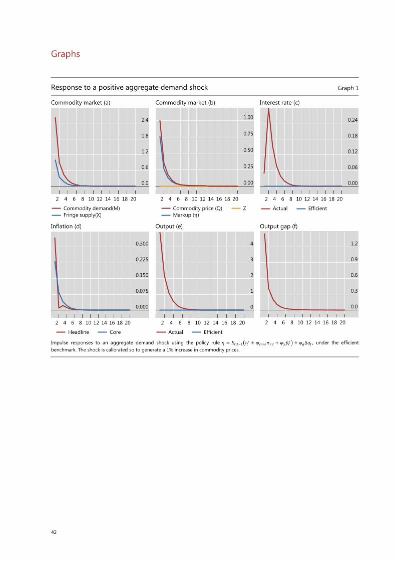
42

Graphs

Response to a positive aggregate demand shock Graph 1

Commodity market (a) Commodity market (b) Interest rate (c)

Inflation (d) Output (e) Output gap (f)

Impulse responses to an aggregate demand shock using the policy rule = | + , + + ∆ , under the efficient benchmark. The shock is calibrated so to generate a 1% increase in commodity prices.

2.4

1.8

1.2

0.6

0.0

2018161412108642

Commodity demand(M)Fringe supply(X)

1.00

0.75

0.50

0.25

0.00

2018161412108642

Commodity price (Q)Markup (η)

Z

0.24

0.18

0.12

0.06

0.00

2018161412108642

Actual Efficient

0.300

0.225

0.150

0.075

0.000

2018161412108642

Headline Core

4

3

2

1

0

2018161412108642

Actual Efficient

1.2

0.9

0.6

0.3

0.0

2018161412108642

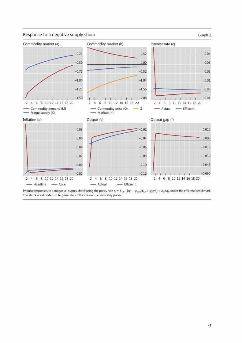
43

Response to a negative supply shock Graph 2

Commodity market (a) Commodity market (b) Interest rate (c)

Inflation (d) Output (e) Output gap (f)

Impulse responses to a (negative) supply shock using the policy rule = | + , + + ∆ , under the efficient benchmark.The shock is calibrated so to generate a 1% increase in commodity prices.

–0.25

–0.50

–0.75

–1.00

–1.25

–1.502018161412108642

Commodity demand (M)Fringe supply (X)

0.52

0.00

–0.52

–1.04

–1.56

–2.082018161412108642

Commodity price (Q)Markup (η)

Z

0.04

0.03

0.02

0.01

0.00

–0.012018161412108642

Actual Efficient

0.08

0.06

0.04

0.02

0.00

–0.022018161412108642

Headline Core

–0.02

–0.04

–0.06

–0.08

–0.10

–0.122018161412108642

Actual Efficient

0.015

0.000

–0.015

–0.030

–0.045

–0.0602018161412108642

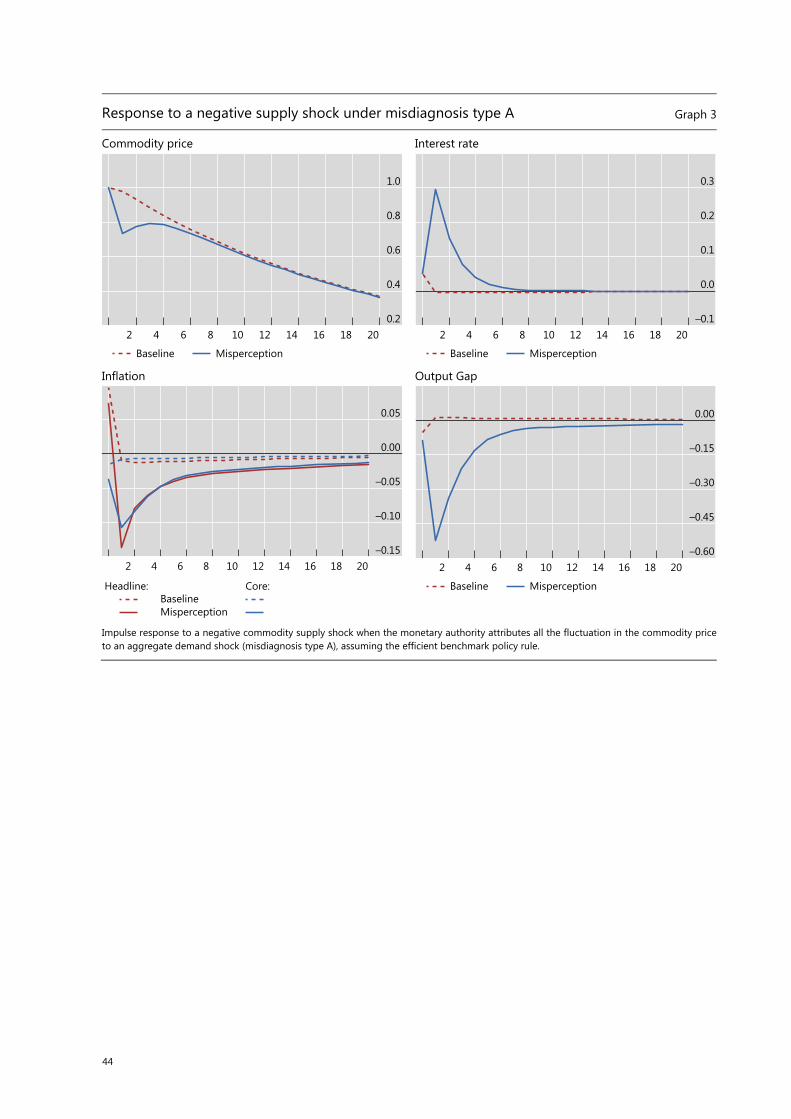
44

Response to a negative supply shock under misdiagnosis type A Graph 3

Commodity price Interest rate

Inflation Output Gap

Impulse response to a negative commodity supply shock when the monetary authority attributes all the fluctuation in the commodity price to an aggregate demand shock (misdiagnosis type A), assuming the efficient benchmark policy rule.

1.0

0.8

0.6

0.4

0.22018161412108642

Baseline Misperception

0.3

0.2

0.1

0.0

–0.12018161412108642

Baseline Misperception

0.05

0.00

–0.05

–0.10

–0.152018161412108642

Baseline Misperception

Headline: Core:

0.00

–0.15

–0.30

–0.45

–0.602018161412108642

Baseline Misperception

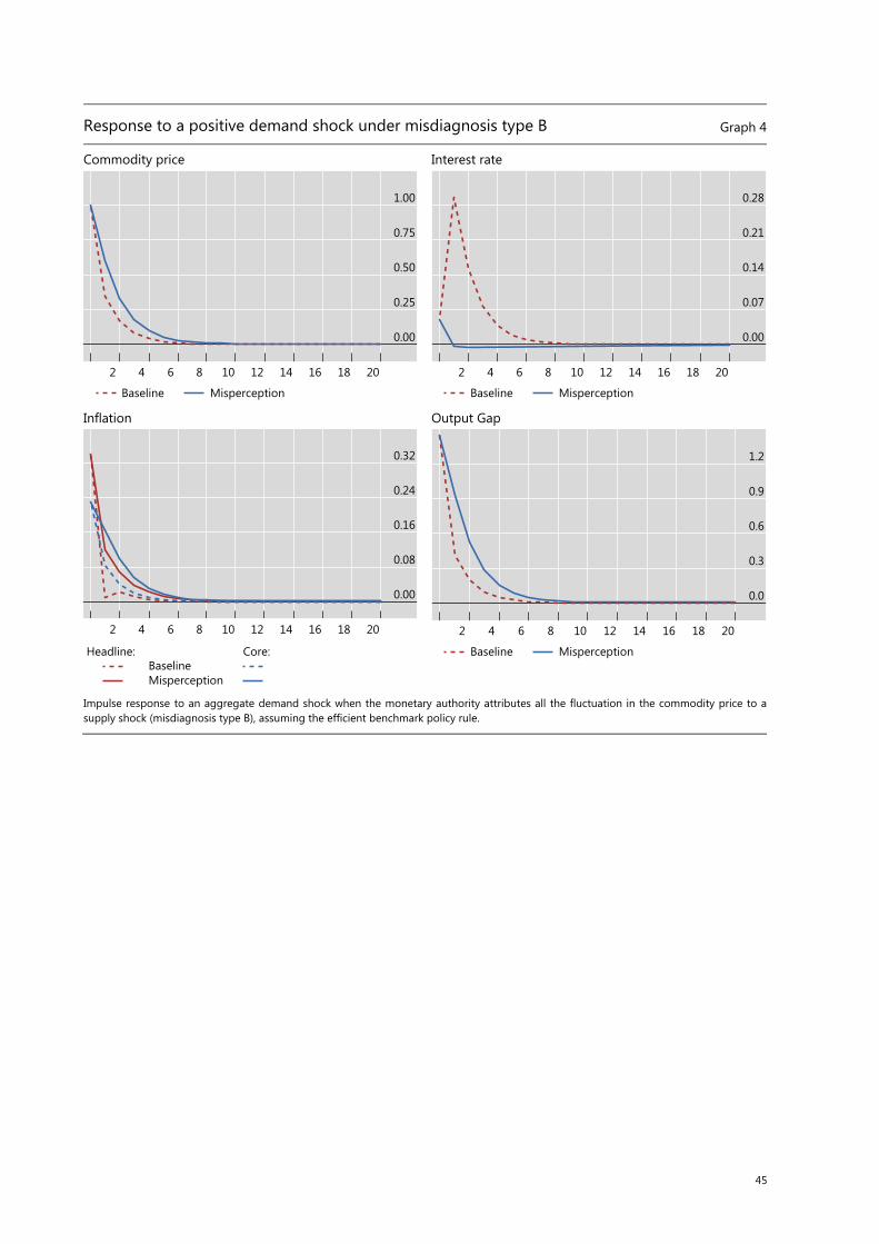
45

Response to a positive demand shock under misdiagnosis type B Graph 4

Commodity price Interest rate

Inflation Output Gap

Impulse response to an aggregate demand shock when the monetary authority attributes all the fluctuation in the commodity price to a supply shock (misdiagnosis type B), assuming the efficient benchmark policy rule.

1.00

0.75

0.50

0.25

0.00

2018161412108642

Baseline Misperception

0.28

0.21

0.14

0.07

0.00

2018161412108642

Baseline Misperception

0.32

0.24

0.16

0.08

0.00

2018161412108642

Baseline Misperception

Headline: Core:

1.2

0.9

0.6

0.3

0.0

2018161412108642

Baseline Misperception

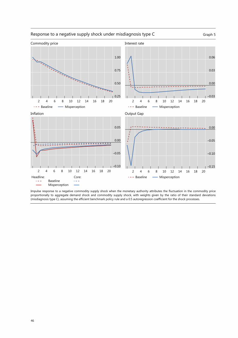
46

Response to a negative supply shock under misdiagnosis type C Graph 5

Commodity price Interest rate

Inflation Output Gap

Impulse response to a negative commodity supply shock when the monetary authority attributes the fluctuation in the commodity priceproportionally to aggregate demand shock and commodity supply shock, with weights given by the ratio of their standard deviations (misdiagnosis type C), assuming the efficient benchmark policy rule and a 0.5 autoregression coefficient for the shock processes.

1.00

0.75

0.50

0.252018161412108642

Baseline Misperception

0.06

0.03

0.00

–0.032018161412108642

Baseline Misperception

0.05

0.00

–0.05

–0.102018161412108642

Baseline Misperception

Headline: Core:

0.00

–0.05

–0.10

–0.152018161412108642

Baseline Misperception

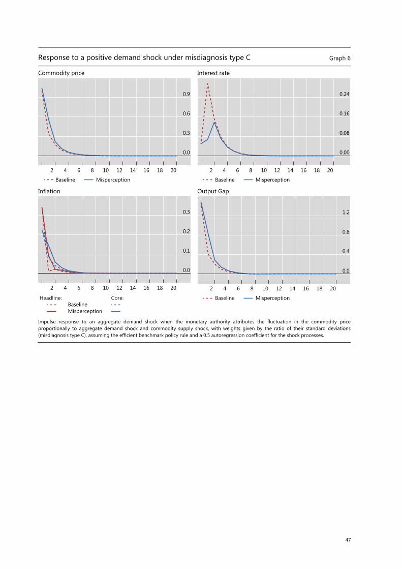
47

Response to a positive demand shock under misdiagnosis type C Graph 6

Commodity price Interest rate

Inflation Output Gap

Impulse response to an aggregate demand shock when the monetary authority attributes the fluctuation in the commodity priceproportionally to aggregate demand shock and commodity supply shock, with weights given by the ratio of their standard deviations (misdiagnosis type C), assuming the efficient benchmark policy rule and a 0.5 autoregression coefficient for the shock processes.

0.9

0.6

0.3

0.0

2018161412108642

Baseline Misperception

0.24

0.16

0.08

0.00

2018161412108642

Baseline Misperception

0.3

0.2

0.1

0.0

2018161412108642

Baseline Misperception

Headline: Core:

1.2

0.8

0.4

0.0

2018161412108642

Baseline Misperception

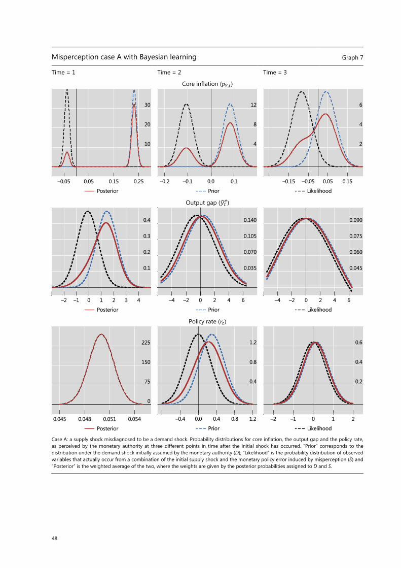
48

Misperception case A with Bayesian learning Graph 7

Time = 1 Time = 2 Time = 3

Core inflation (𝑝𝑝𝑌𝑌,𝑡𝑡)

Output gap (𝑦𝑦�𝑡𝑡𝑒𝑒)

Policy rate (𝑟𝑟𝑡𝑡)

Case A: a supply shock misdiagnosed to be a demand shock. Probability distributions for core inflation, the output gap and the policy rate, as perceived by the monetary authority at three different points in time after the initial shock has occurred. “Prior” corresponds to the distribution under the demand shock initially assumed by the monetary authority (D); “Likelihood” is the probability distribution of observed variables that actually occur from a combination of the initial supply shock and the monetary policy error induced by misperception (S) and “Posterior” is the weighted average of the two, where the weights are given by the posterior probabilities assigned to D and S.

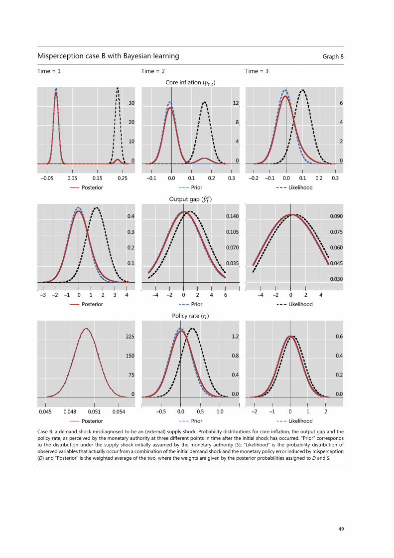
49

Misperception case B with Bayesian learning Graph 8

Time = 1 Time = 2 Time = 3

Core inflation (𝑝𝑝𝑌𝑌,𝑡𝑡)

Output gap (𝑦𝑦�𝑡𝑡𝑒𝑒)

Policy rate (𝑟𝑟𝑡𝑡)

Case B: a demand shock misdiagnosed to be an (external) supply shock. Probability distributions for core inflation, the output gap and the policy rate, as perceived by the monetary authority at three different points in time after the initial shock has occurred. “Prior” corresponds to the distribution under the supply shock initially assumed by the monetary authority (S); “Likelihood” is the probability distribution of observed variables that actually occur from a combination of the initial demand shock and the monetary policy error induced by misperception (D) and “Posterior” is the weighted average of the two, where the weights are given by the posterior probabilities assigned to D and S.

50

A. Model equations

A.1 Commodity-importing country

A.1.1 Aggregate demand

Resource constraint (AD): ,,

Y t

t t t Y tt

PY C Q

P= + M .

IS equation: 1

1

1

11 t

t tt t

CE R

Cb

-+

+

é ùæ öæ öê ú÷ ÷ç ç÷ ÷= ç çê ú÷ ÷ç ç÷ ÷ç çPê úè øè øê úë û

.

Total consumption: ( ) ( )1

, ,t Y t C tC C

g g-

= M .

Relative price final goods/total consumption goods,( ),/

Y t tP P :

1

,1

Y t

t

t

PQ

P

g

g

-æ ö÷ç ÷ç ÷= ç ÷ç ÷ç ÷çè ø.

A.1.2 Aggregate supply

Total inflation: ( )1

,1

tt Y t t

t

Q

Q

gg-

-

æ ö÷ç ÷çP = P P ÷ç ÷÷çè ø.

Core inflation Phillips Curve:

( ) ( ) 11, 1 1t t t t Y t tD Y C E Dqb

--+ +

é ù= + Pê úë û

,

( ) ( )1, 1 1t t t t t Y t tN Y C MC E Nm qb

-+ +

é ù= + Pê úë û

,

( )1

1, 1 (1 ) tY t

t

N

Dq q

-- æ ö÷ç ÷P = - - ç ÷ç ÷çè ø

.

Price dispersion (only second-order effects):

( ) ( )1 ,1 tt t Y t

t

N

D

ee

q q-

-

æ ö÷ç ÷D = - + D Pç ÷ç ÷çè ø.

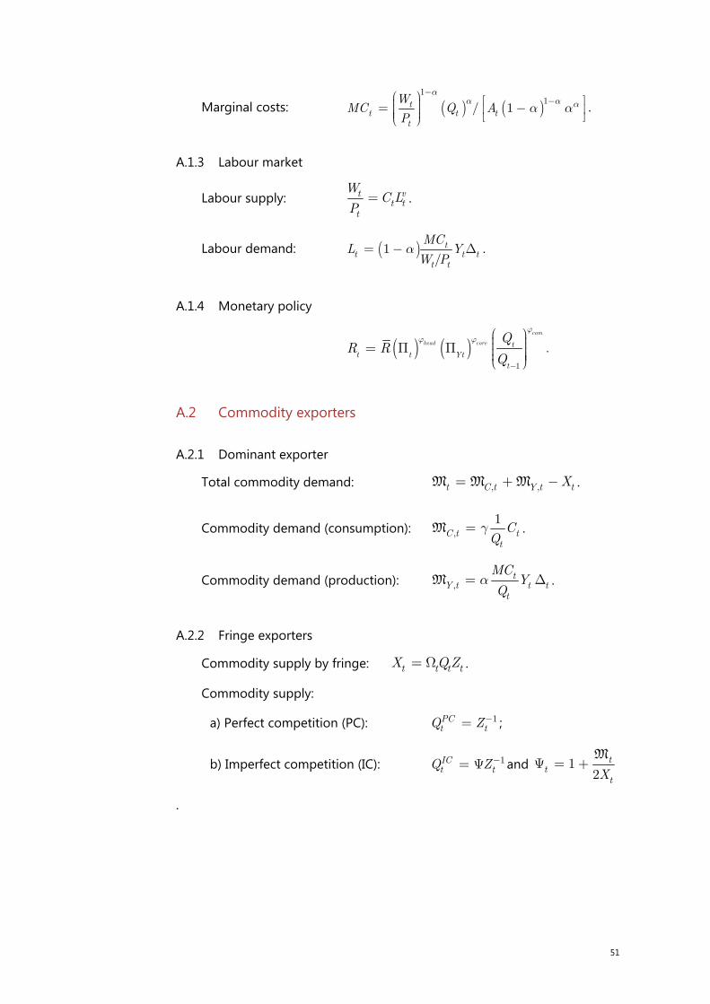
51

Marginal costs: ( ) ( )1

1/ 1t

t t tt

WMC Q A

P

aa a aa a

--æ ö é ù÷ç ÷= -ç ê ú÷ç ÷ç ë ûè ø

.

A.1.3 Labour market

Labour supply: vtt t

t

WC L

P= .

Labour demand: ( )1/t

t t tt t

MCL Y

W Pa= - D .

A.1.4 Monetary policy

( ) ( )1

com

head core tt t Yt

t

QR R

Q

jj j

-

æ ö÷ç ÷ç= P P ÷ç ÷÷çè ø.

A.2 Commodity exporters

A.2.1 Dominant exporter

Total commodity demand: , ,t C t Y t tX= + -M M M .

Commodity demand (consumption): ,1

C t tt

CQ

g=M .

Commodity demand (production): ,t

Y t t tt

MCY

Qa= DM .

A.2.2 Fringe exporters

Commodity supply by fringe: t t t tX QZ= W .

Commodity supply:

a) Perfect competition (PC): 1PCt tQ Z-= ;

b) Imperfect competition (IC): 1ICt tQ Z-= Y and 1

2t

ttX

Y = +M

.

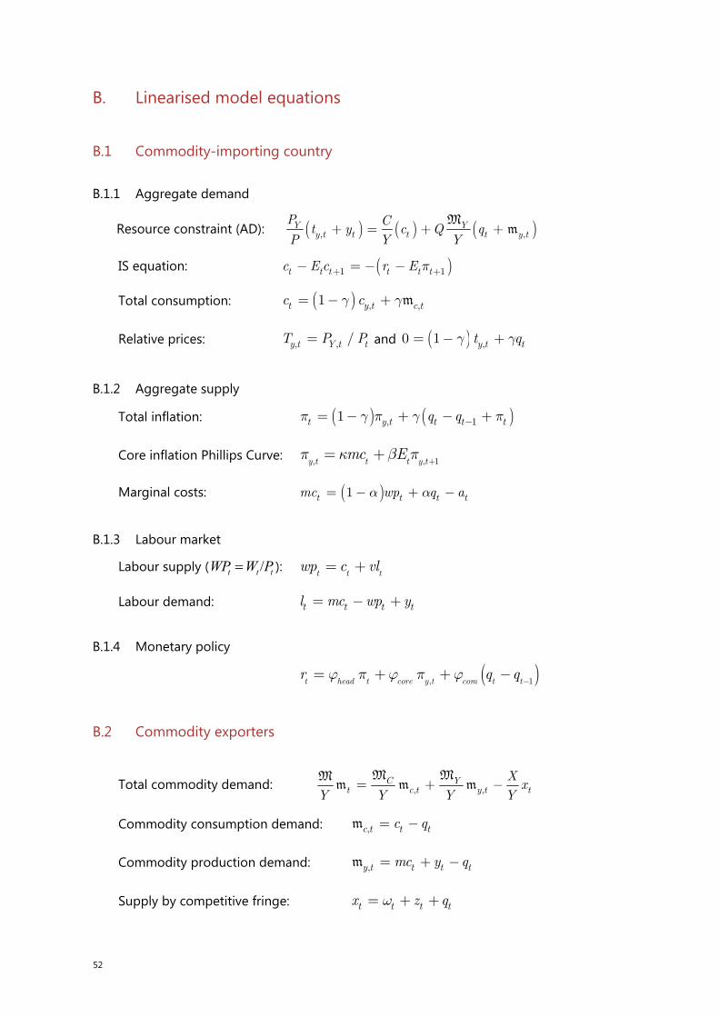
52

B. Linearised model equations

B.1 Commodity-importing country

B.1.1 Aggregate demand

Resource constraint (AD): ( ) ( ) ( ), ,Y Y

y t t t t y t

P Ct y c Q q

P Y Y+ = + +

Mm

IS equation: ( )1 1t t t t t tc E c r E p+ +- = - -

Total consumption: ( ) , ,1t y t c tc cg g= - + m

Relative prices: , , /y t Y t tT P P= and ( ) ,0 1 y t tt qg g= - +

B.1.2 Aggregate supply

Total inflation: ( ) ( ), 11t y t t t tq qp g p g p-= - + - +

Core inflation Phillips Curve: , , 1y t t t y tmc Ep k b p += +

Marginal costs: ( )1t t t tmc wp q aa a= - + -

B.1.3 Labour market

Labour supply ( /t t tWP W P ): t t t

wp c vl= +

Labour demand: t t t tl mc wp y= - +

B.1.4 Monetary policy

( ), 1t head t core y t com t tr q qj p j p j

-= + + -

B.2 Commodity exporters

Total commodity demand: , ,C Y

t c t y t tXx

Y Y Y Y= + -M MM

m m m

Commodity consumption demand: ,c t t tc q= -m

Commodity production demand: ,y t t t tmc y q= + -m

Supply by competitive fringe: t t t tx z qw= + +

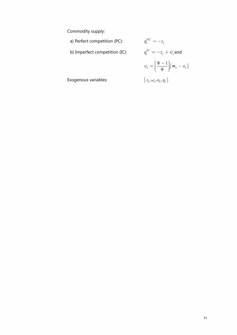
53

Commodity supply:

a) Perfect competition (PC): PCt tq z= -

b) Imperfect competition (IC): t t

IC

tq z y=- + and

( )1t t txy

æ öY - ÷ç= -÷ç ÷ç ÷è øYm

Exogenous variables: ( ), , ,t t t tz a gw

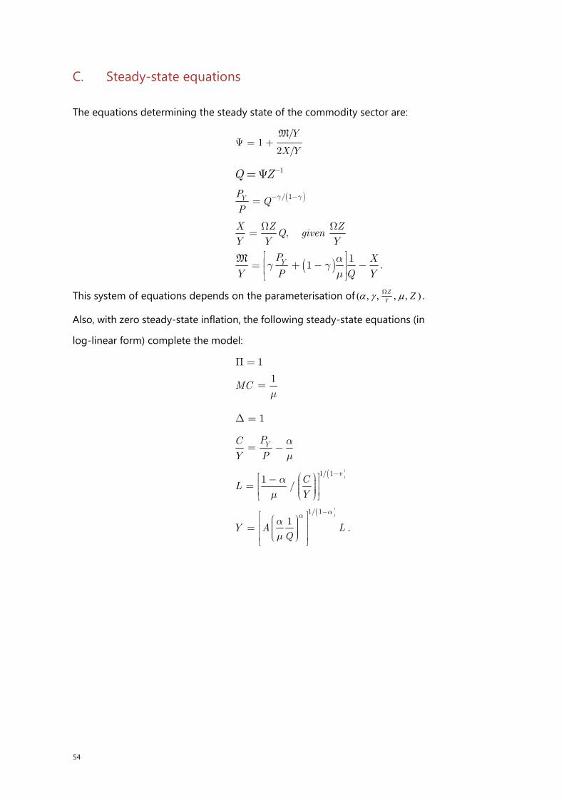
54

C. Steady-state equations

The equations determining the steady state of the commodity sector are:

/

12 /

Y

X YY = +

M

1Q Z-= Y

( )/ 1YP QP

g g- -=

, giX Z Z

QY Y Y

venW W

=

( ) 11 .YP X

Y P Q Y

ag g

m

é ùê ú= + - -ê úë û

M

This system of equations depends on the parameterisation of ( , , , , )ZY Z .

Also, with zero steady-state inflation, the following steady-state equations (in

log-linear form) complete the model:

1P =

1

MCm

=

1D =

YPC

Y P

am

= -

( )1/ 1

1/

vC

LY

am

-é æ öù- ÷çê ú= ÷ç ÷ç ÷ê úè øë û

( )1/ 1

1Y A L

Q

aaam

-é ùæ öê ú÷ç= ÷çê ú÷ç ÷è øê úë û.

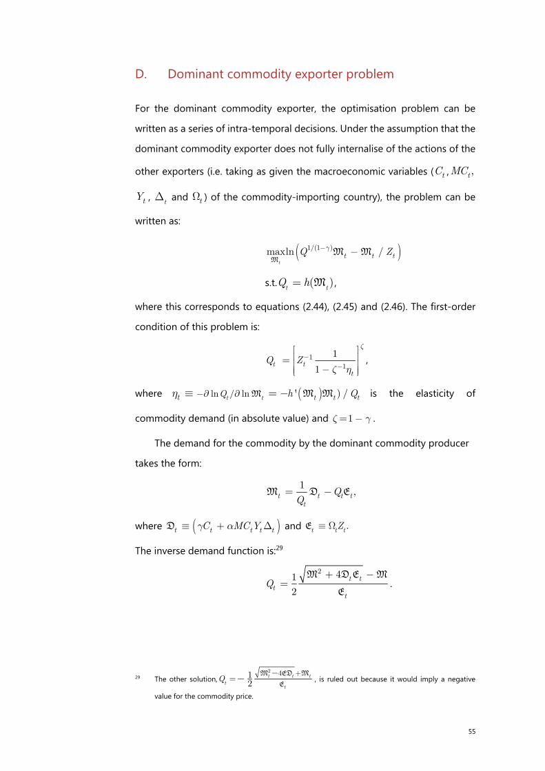
55

D. Dominant commodity exporter problem

For the dominant commodity exporter, the optimisation problem can be

written as a series of intra-temporal decisions. Under the assumption that the

dominant commodity exporter does not fully internalise of the actions of the

other exporters (i.e. taking as given the macroeconomic variables ( tC , ,tMC

tY , t

D and tW ) of the commodity-importing country), the problem can be

written as:

( )1/(1 )maxln /t

t t tQ Zg- -M

MM

s.t. ( )t tQ h= M ,

where this corresponds to equations (2.44), (2.45) and (2.46). The first-order

condition of this problem is:

11

1

1t t

t

Q Z

z

z h-

-

é ùê ú= ê ú-ê úë û

,

where ( )ln ln/ )' /t t t t tt Q h Qh -¶ ¶º -=M M M is the elasticity of

commodity demand (in absolute value) and 1z g= - .

The demand for the commodity by the dominant commodity producer

takes the form:

1

,t t t tt

QQ

= -M D E

where ( )t t t t tC MC Yg aº + DD and .t t tZº WE

The inverse demand function is:29

2 41

2t t

tt

Q+ -

=M D E M

E.

29 The other solution,2 41

2t tt

ttQ

+=

-- EDM M

E, is ruled out because it would imply a negative

value for the commodity price.

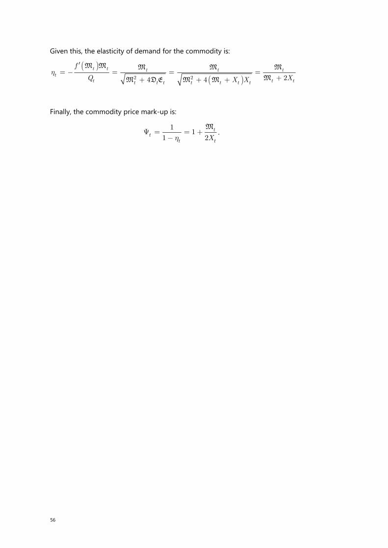
56

Given this, the elasticity of demand for the commodity is:

( )( )2 2 24 4

t t t t tt

t t tt t t t t t t

f

Q XX Xh

¢= - = = =

++ + +

M M M M M

MM MDE M

Finally, the commodity price mark-up is:

1

11 2

tt

t tXh=Y = +

-M

.

57

E. Deriving the benchmark level for final goods output

This appendix derives the benchmark level of final goods output as a function

of variables ,tMCt

D and tQ , starting from the aggregate production

function: 1, .t t t Y tY AL a a-= M

First, the labour input, tL , is recast in terms of these variables of interest.

Substituting the labour supply equation (2.6) into the aggregate lab ,t our

demand equation (2.28) and solving for tL yields:

( )( )1/ 1

.1v

tt t t

t

MCL Y

Ca

+é ùê ú= - Dê úë û

ReplacingtC using the aggregate demand equation (2.50) along with

equations (2.7), (2.8) and (2.49) yield the following form:

( )

( )

,

1/ 1

,

1 .Y t

t

v

tt t t

t t Y t

P

P

MCL Y

Y Qa

+é ùê úê ú= - Dê úê ú-ë û

M

Substituting the commodity demand for output (2.29), making use of

equation (2.10), to solve for tQ achieves the desired result:

( )

( )

( )1/ 1

/(1 )

1.

v

tt t

t t t

MCL

Q MCg g

a

a

+

- -

é ù-ê ú= Dê ú

ê ú- Dê úë û

Second, the commodity demand in equation (2.28) is plugged into the

aggregate output equation (2.29), giving the following form fortY :

( ) ( )1/ 1 / 1

.t tt t t

t t

A MCY L

Q

a a a

a- -æ ö æ ö÷ ÷ç ç÷ ÷= Dç ç÷ ÷ç ç÷ ÷ç çDè ø è ø

Finally, substituting the labour input from the equation above

completes the derivation:

( ) ( )

( )

( )( )

1/ 11/ 1 / 1

/(1 )

1.

v

tt tt t t

t tt t t

MCA MCY

QQ MC

a a a

g g

aa

a

+- -

- -

é ù-æ ö æ öê ú÷ ÷ç ç÷ ÷ê ú= D Dç ç÷ ÷ç ç÷ ÷ç çê úDè ø è ø- Dê úë û

58

F. The impact of a small country on commodity prices

Consider countries indexed by . If they are all equal in the production

technology the demand for commodity of each country is:

, = , , ∆If all countries do not deviate from the cooperative equilibrium, the

world demand for commodity ( , ) is:

, = , , ∆ = , , ∆Solving for the commodity price:

, = , ∆,If one country ( ) deviates, the world demand ( , ) becomes:

, = , , ∆ + , , ∆= − 1 , , ∆ + , , ∆

Dividing for the cooperative equilibrium ( , ):

,, = − 1 , , ∆, , ∆ + , , ∆

, , ∆With simple algebra:

,, = − 1 ,, + , , ∆, , ∆

When → ∞, ,, → ,, = 1 or equivalently , → , . Therefore, a

deviation from the cooperative equilibrium of one small country does not

influence the global commodity price.