money, interest rates, and economic activity · 28 money, interest rates, and economic activity...
TRANSCRIPT
28 Money, Interest Rates, and Economic Activity
CHAPTER OUTLINE LEARNING OBJECTIVES (LO)
In this chapter you will learn
28.1 UNDERSTANDING BONDS 1 why the price of a bond is inversely related to the market interest rate.
28.2 THE THEORY OF MONEY DEMAND 2 how to describe how the demand for money depends on the interest rate, the price level, and real GDP.
28.3 MONETARY EQUILIBRIUM AND NATIONAL INCOME 3 how monetary equilibrium determines the interest rate in the short run.
4 how to describe the transmission mechanism of monetary policy.
28.4 THE STRENGTH OF MONETARY FORCES 5 the difference between the short-run and long-run effects of monetary policy.
6 how to describe under what conditions monetary policy is most effective in the short run.
IN Chapter 27 , we learned how the commercial banking system multiplies a given amount of reserves into deposit money and thus influences the nation’s money supply. We also learned that because the Bank of Canada can set the amount of commercial-bank reserves, it too has an influence on the money supply. What we have not yet discussed, however, is how the Bank influences the amount of reserves . We will leave that discussion until the next chapter, when we examine Canadian monetary policy. For now, just think of the nation’s money supply as being determined jointly by the actions of the Bank of Canada and the commercial banking system.
In this chapter, we develop a theory to explain how money affects the economy. Understanding the
role of money, however, requires an understand-ing of the interaction of money supply and money demand. To examine the nature of money demand, we begin by examining how households decide to divide their total holdings of assets between money and interest-earning assets (which here are called “bonds”). Once that is done, we put money supply and money demand together to examine monetary equilibrium. Only then can we ask how changes in the supply of money or in the demand for money affect the economy in the short term—interest rates, real GDP, and the price level. We begin with a dis-cussion of the relationship between bond prices and interest rates.
M28_RAGA8785_14_SE_C28.indd 1 04/10/12 12:49 PM

2 PART 10 : MONEY, BANK ING , AND MONETARY POL IC Y
28.1 Understanding Bonds
At any moment, households have a stock of financial wealth that they hold in several forms. Some of it is money in the bank or in the wallet. Some may be in Treasury bills and bonds, which are IOUs issued by the government or corporations. Some may be in equity, meaning ownership shares of a company.
To simplify our discussion, we will group financial wealth into just two categor-ies, which we call “money” and “bonds.” By money we mean all assets that serve as a medium of exchange—that is, paper money, coins, and bank deposits that can be transferred on demand by cheque or electronic means. By bonds we mean all other forms of financial wealth; this includes interest-earning financial assets and claims on real capital (equity). This simplification is useful because it emphasizes the important distinction between interest-earning and non–interest-earning assets, a distinction that is central for understanding the demand for money.
Before discussing how individuals decide to divide their assets between money and bonds, we need to make sure we understand what bonds are and how they are priced. This requires an understanding of present value .
Present Value and the Interest Rate
A bond is a financial asset that promises to make one or more specified payments at specified dates in the future. The present value ( PV ) of any asset refers to the value now of the future payments that the asset offers. Present value depends on the market inter-est rate because when we calculate present value, the interest rate is used to discount the value of the future payments to obtain their present value. Let’s consider two examples to illustrate the concept of present value.
A Single Payment One Year Hence We start with the simplest case. What is the value now of a bond that will return a single payment of $100 in one year’s time?
Suppose the market interest rate is 5 percent. Now ask how much you would have to lend out at that interest rate today in order to have $100 a year from now. If we use PV to stand for this unknown amount, we can write PV * (1.05) = +100. Thus, PV = +100>1.05 = +95.24 .1 This tells us that the present value of $100 receivable in one year’s time is $95.24; if you lend out $95.24 for one year at 5 percent interest you will get back the original $95.24 that you lent (the principal) plus $4.76 in interest, which makes $100.
We can generalize this relationship with a simple equation. If R1 is the amount we receive one year from now and i is the annual interest rate, the present value of R1 is
PV =R1
1 + i
If the interest rate is 7 percent (i = 0.07) and the bond pays $100 in one year (R1 = +100), the present value of that bond is PV = +100>1.07 = +93.46. Notice
Economists often simplify the analysis of financial assets by considering only two types of assets—non– interest-bearing “money” and interest-bearing “bonds.”
present value ( PV ) The value now of one or more payments or receipts made in the future; often referred to as discounted
present value .
1 Notice that in this type of formula, the interest rate is expressed as a decimal fraction where, for example, 5 percent is expressed as 0.05, so 1 + i = 1.05.
M28_RAGA8785_14_SE_C28.indd 2 04/10/12 12:49 PM

CHAPTER 28 : MONEY, I N TEREST RATES, AND ECONOMIC AC T I V I T Y 3
that, when compared with the previous numerical example, the higher market interest rate leads to a lower present value. The future payment of $100 gets discounted at a higher rate and so is worth less at the present time.
A Sequence of Future Payments Now consider a more complicated case, but one that is actually more typical. Many bonds promise to make “coupon” payments every year and then return the face value of the bond at the end of the term of the loan. For example, imagine a three-year bond that promises to repay the face value of $1000 in three years, but will also pay a 10 percent coupon payment of $100 at the end of each of the three years that the bond is held. How much is this bond worth now? We can compute the present value of this bond by adding together the present values of each of the payments. If the market interest rate is 7 percent, the present value of this bond is
PV =+1001.07
+
+100
(1.07)2 +
+1100
(1.07)3
The first term is the value today of receiving $100 one year from now. The second term is the value today of receiving the second $100 payment two years from now. Note that we discount this second payment twice—once from Year 2 to Year 1, and once again from Year 1 to now—and thus the denominator shows an interest rate of 7 percent compounded for two years. Finally, the third term shows the value today of the $1100 repayment ($1000 of face value plus $100 of coupon payment) three years from now. The present value of this bond is
PV = +93.46 + +87.34 + +897.93
= +1078.73
In general, any asset that promises to make a sequence of payments for T periods into the future of R1, R2, c, and so on, up to R T has a present value given by
PV =R1
1 + i+
R2
(1 + i)2 + g +
RT
(1 + i)T
It is useful to try another example. Let’s continue with the case in which the bond repays its face value of $1000 three years from now and makes three $100 coupon payments at the end of each year the bond is held. But this time we assume the market interest rate is 9 percent. In this case, the present value of the bond is
PV =+1001.09
+
+100
(1.09)2 +
+1100
(1.09)3
= +91.74 + +84.17 + +849.40
= +1025.31
Notice that when the market interest rate is 9 percent, the present value of the bond is lower than the present value of the same bond when the market interest rate is 7 percent. The higher interest rate implies that any future payments are discounted at a higher rate and thus have a lower present value.
A General Relationship There are many types of bonds. Some make no coupon pay-ments and only a single payment (the “face value”) at some point in the future. This is the case for short-term government bonds called Treasury bills. Other bonds, typically longer-term government or corporate bonds, make regular coupon payments as well as
M28_RAGA8785_14_SE_C28.indd 3 04/10/12 12:49 PM

4 PART 10 : MONEY, BANK ING , AND MONETARY POL IC Y
a final payment of the bond’s face value. Though there are many types of bonds, they all have one thing in common: They promise to make some payment or sequence of payments in the future. Because bonds make payments in the future, their present value is negatively related to the market interest rate.
2 We ignore for now the possibility that the issuer of the bond will default and thereby fail to make some or all of the future payments. If such a risk does exist, it will reduce the expected present value of the bond and thus reduce the price that buyers will be prepared to pay. We address bond riskiness shortly.
The present value of a bond is the most someone would be willing to pay now to own the bond’s future stream of payments. 2
The present value of any bond that promises a future payment or sequence of future payments is negatively related to the market interest rate.
Present Value and Market Price
Most bonds are bought and sold in financial markets in which there are large numbers of both buyers and sellers. The present value of a bond is important because it estab-lishes the price at which a bond will be exchanged in the financial markets.
To understand this concept, let us return to our example of a bond that promises to pay $100 one year from now. When the interest rate is 5 percent, the present value of this bond is $95.24. To see why this is the maximum that anyone would pay for this bond, suppose that some sellers offer to sell the bond at some other price, say, $98. If, instead of paying this amount for the bond, a potential buyer lends $98 out at 5 percent interest, he or she would have at the end of one year more than the $100 that the bond will produce. (At 5 percent interest, $98 yields $4.90 in interest, which when added to the principal makes $102.90.) Clearly, no well-informed individual would pay $98—or, by the same reasoning, any sum in excess of $95.24—for the bond. Thus, at any price above the bond’s present value, the lack of demand will cause the price to fall.
Now suppose the bond is offered for sale at a price less than $95.24, say, $90. A potential buyer could borrow $90 to buy the bond and would pay $4.50 in interest on the loan. At the end of the year, the bond yields $100. When this is used to repay the $90 loan and the $4.50 in interest, $5.50 is left as profit. Clearly, it would be worth-while for someone to buy the bond at the price of $90 or, by the same argument, at any price less than $95.24. Thus, at any price below the bond’s present value, the abun-dance of demand will cause the price to rise.
This discussion should make clear that the present value of an asset determines its equilibrium market price. If the market price of any asset is greater than the present value of its income stream, no one will want to buy it, and the resulting excess supply will push down the market price. If the market price is below its present value, there will be a rush to buy it, and the resulting excess demand will push up the market price. When the bond’s market price is exactly equal to its present value, there is no pressure for the price to change.
M28_RAGA8785_14_SE_C28.indd 4 04/10/12 12:49 PM

CHAPTER 28 : MONEY, I N TEREST RATES, AND ECONOMIC AC T I V I T Y 5
Interest Rates, Bond Prices, and Bond Yields
We now have two relationships that can be put together to tell us about the link between the market interest rate and bond prices. Let’s restate these two relationships.
1. The present value of any given bond is negatively related to the market interest rate.
2. A bond’s equilibrium market price will be equal to its present value.
Putting these two relationships together, we come to a key relationship:
The equilibrium market price of any bond is the present value of the income stream that it produces.
An increase in the market interest rate leads to a fall in the price of any given bond. A decrease in the market interest rate leads to an increase in the price of any given bond.
An increase in the market interest rate will reduce bond prices and increase bond yields. A reduction in the market interest rate will increase bond prices and reduce bond yields. Therefore, market interest rates and bond yields tend to move together.
Remember that a bond is a financial investment for the purchaser. The cost of the investment is the price of the bond, and the return on the investment is the sequence of future payments. Thus, for a given sequence of future payments, a lower bond price implies a higher rate of return on the bond, or a higher bond yield.
To illustrate the yield on a bond, consider a simple example of a bond that promises to pay $1000 two years from now. If you purchase this bond for $857.34, your return on your investment will be 8 percent per year because $857.34 compounded for two years at 8 percent will yield $1000 in two years.
+857.34 * (1.08)2 = +1000
In other words, your yield on the bond will be 8 percent per year. Notice that we are making a distinction between the concept of the yield on a bond
and the market interest rate . The bond yield is a function of the sequence of payments and the bond price. The market interest rate is the rate at which you can borrow or lend money in the credit market.
Although they are logically distinct from each other, there is a close relationship between the market interest rate and bond yields. A rise in the market interest rate will lead to a decline in the present value of any bond and thus to a decline in its equilib-rium price. As the bond price falls, its yield naturally rises. Thus, we see that market interest rates and bond yields tend to move in the same direction.
Because of this close relationship between bond yields and market interest rates, economists discussing the role of money in the macroeconomy typically refer to “the”
M28_RAGA8785_14_SE_C28.indd 5 04/10/12 12:49 PM

6 PART 10 : MONEY, BANK ING , AND MONETARY POL IC Y
interest rate—or perhaps to “interest rates” in general—rather than to any specific interest rate among the many different rates corresponding to the many different finan-cial assets. Since these rates all tend to rise or fall together, it is a very useful simplification to refer only to “the” inter-est rate, meaning the rate of return that can be earned by holding interest-earning assets rather than money.
Bond Riskiness
We have been discussing present values and bond prices under the assumption that the bond is risk free— that is, that the coupon payments and the repayment of principal
are absolutely certain. In reality, however, there is some chance that bond issuers will be unable to make some or all of these payments. In the face of this possibility, purchasers of bonds reduce the price they are prepared to pay by an amount that reflects the likelihood of non-repayment.
It follows that not all changes in bond yields are caused by changes in market inter-est rates. Sometimes the yields on specific bonds change because of a change in their perceived riskiness . For example, if some event increases the likelihood that a specific corporate bond issuer will soon go bankrupt, bond purchasers will revise downward the expected present value of the issuer’s bonds. As a result, the demand for the bond will fall and its equilibrium price will decline. As the price falls, the bond’s yield will rise—the higher bond yield now reflecting the greater riskiness of the bond.
An increase in the riskiness of any bond leads to a decline in its expected present value and thus to a decline in the bond’s price. The lower bond price implies a higher bond yield.
It is rare in Canada that government bonds are perceived as risky, but in recent years some bonds issued by some southern European countries have been viewed as high-risk assets, and this riskiness has been reflected in high bond yields. In general, however, since governments have the power to collect revenue through taxation, it is unusual for a government bond to be viewed as a risky asset. More usual at any given time is specific corporations that are believed to be in precarious financial situations and thus their bonds are perceived to be risky assets. As a result, there are often very high yields (low bond prices) on specific corporate bonds. Applying Economic Con-cepts 28-1 discusses the relationship among bond prices, bond yields, riskiness, and term to maturity of government and corporate bonds.
28.2 The Theory of Money Demand
Our discussion of bonds, bond prices, and interest rates leads us to a theory that explains how individuals allocate their current stock of financial wealth between “bonds” and “money.” An individual’s decision to hold more bonds is at the same time a decision to hold less money, and the decision to hold fewer bonds is a decision to hold more money.
M28_RAGA8785_14_SE_C28.indd 6 04/10/12 12:49 PM

CHAPTER 28 : MONEY, I N TEREST RATES, AND ECONOMIC AC T I V I T Y 7
APPLYING ECONOMIC CONCEPTS 28-1
Understanding Bond Prices and Bond Yields
Various kinds of bonds are traded every day, and they differ in terms of the issuer, price, yield, riskiness, and term to maturity. We focus here on how to understand these bond characteristics.
How to Read the Bond Tables
The accompanying table shows seven bond listings just as they appeared on www.globeinvestor.com on June 22, 2012. The five columns are as follows:
1. Issuer. This is the issuer of the bond—that is, the borrower of the money. The fi rst fi ve bonds shown are issued by the Government of Canada. The last two are issued by large private-sector fi rms.
2. Coupon. This is the coupon rate—the annual rate of interest that the bond pays before it matures. For example, a 6 percent coupon rate means that the bond-holder (the lender) will receive 6 percent of the face value of the bond every year until the bond matures.
3. Maturity. This is when the bond matures and the face value is repaid to the bondholder. All debt obli-gations are then fulfi lled.
4. Price. This is the market price of the bond (on June 22, 2012), expressed as the price per $100 of face value. For example, a price of $103.93 means that for every $100 of face value, the purchaser must pay $103.93. When the price is greater than $100, we say there is a premium ; when the price is less than $100, we say the bond is selling at a discount .
5. Yield. This is the rate of return earned by the bond-holder if the bond is bought at the current price and held to maturity, earning all regular coupon payments.
Issuer Coupon
(%) Maturity Price ($)
Yield (%)
1. Canada 5.25 June 1, 2013 103.93 1.01
2. Canada 2.50 Sept 1, 2013 101.73 1.03
3. Canada 4.00 June 1, 2016 110.62 1.22
4. Canada 9.75 June 1, 2021 167.57 1.60
5. Canada 8.00 June 1, 2027 175.92 2.06
6. Gaz Metro 5.45 July 12, 2021 120.06 2.91
7. Bell Canada 8.88 April 17, 2026 135.52 5.48
Bond Prices and Yields
Three general patterns can be seen in the table. First, for a given issuer and maturity, there is a positive relationship between the bond price and the coupon rate. Rows 1 and 2,
for example, show two bonds, both issued by the Gov-ernment of Canada and maturing at (almost) the same date in 2013. The common issuer suggests a common risk of non-repayment (in this case a very low risk). The first bond has a 5.25 percent coupon whereas the second has a 2.50 percent coupon. Not surprisingly, the higher coupon payments make the first bond a more attractive asset and thus its market price is higher— $103.93 as compared with $101.73. Note, however, that the implied yield on the two bonds is almost identical. If this weren’t the case, demand would shift toward the high-yield (low-price) bond, driving down the yield (increasing the price) until the two yields were the same.
Second, for a given bond issuer, there is a positive relationship between the bond yield and the term to maturity. This is shown in the first five rows, as yields rise from just over 1 percent on bonds maturing in one year’s time (from the date of the listing) to 2.06 per-cent on bonds maturing in 15 years’ time. This posi-tive relationship is often referred to as the yield curve or the term structure of interest rates. The higher yields on longer-term bonds reflect what is often called a term premium —the higher yield that bondholders must be paid in order to induce them to have their money tied up for longer periods of time.
Third, for a given term to maturity, there is a posi-tive relationship between the bond yield and the per-ceived riskiness of the bond issuer. Compare rows 4 and 6, for example. Both bonds have almost identical matur-ity dates in 2021, but one is issued by the Government of Canada while the other is issued by Gaz Metro Inc. Though it is almost impossible for the Government of Canada to go bankrupt and almost inconceivable that it would default on its debt, it is certainly possible for Gaz Metro to do so. This difference explains the difference in yields. The same is true between rows 5 and 7, where the more than three-percentage-point yield difference is attributable to the higher likelihood of default by Bell Canada than by the Canadian government.
If you run your eyes down the bond tables, you will easily see those corporations viewed by the market as being risky borrowers because the yields on their bonds will be higher—often dramatically so—than the yields on similar-maturity government bonds. For example, in the summer of 2012, when some European banks were experiencing great difficulty, the bonds issued by the Royal Bank of Scotland were selling at such a discount that the implied annual yield was more than 20 percent. Such high yields represent a great investment opportunity only if you are prepared to take the associated risk. Beware!
M28_RAGA8785_14_SE_C28.indd 7 04/10/12 12:49 PM

8 PART 10 : MONEY, BANK ING , AND MONETARY POL IC Y
We can therefore build our theory by considering the desire to hold bonds or by consid-ering the desire to hold money. We follow the tradition among economists by focusing on the desire to hold money. The amount of money that everyone (collectively) wants to hold at any time is called the demand for money .
Three Reasons for Holding Money
Why do firms and households hold money? Our theory offers three reasons. First, households and firms hold money in order to carry out transactions. Economists call this the transactions demand for money. You carry money in your pocket or keep it in a chequing account in order to have it readily available for your upcoming transactions; it would be very inconvenient to have to sell bonds or withdraw money from your GIC (guaranteed investment certificate) every time you wanted to spend. Similarly, firms are continually making expenditures on intermediate inputs and payments to labour, and they keep money available in their chequing accounts to pay these expenses.
A second and related reason firms and households hold money is that they are uncertain about when some expenditures will be necessary, and they hold money as a precaution to avoid the problems associated with missing a transaction. This is referred to as the precautionary demand for money. For example, you might hold some cash because of the possibility that you might need to take an unplanned taxi ride during a rainstorm; a small business may hold cash because of the possibility that it might need the emergency services of a tradesperson, such as a plumber or an electrician. In the days before the invention of ATMs, the precautionary demand for money was quite large, since to be caught on a weekend or away from home without sufficient cash could be a serious matter. Today, this motive for holding money is less important.
The third assumed reason for holding money applies more to large businesses and to professional money managers than to individuals because it involves speculating about how interest rates are likely to change in the future. Economists call this the speculative demand for money. To understand this reason for holding money, recall what we said earlier about the negative relationship between market interest rates and bond prices. If interest rates are expected to rise in the future, bond prices will be expected to fall. Whenever bond prices fall, bondholders experience a decline in the value of their bond holdings. The expectation of increases in future interest rates will therefore lead to the holding of more money (and fewer bonds) now as financial managers adjust their portfolios in order to preserve their values.
A related motive for holding money relates to uncertainty . Commercial banks that are uncertain about their borrowers’ ability to repay loans, or about the riskiness of poten-tial new borrowers, may decide to sacrifice an uncertain rate of return for the safety that comes from holding more cash reserves than normal. Other firms that regularly borrow to finance their operations may choose to hold large cash balances if they are uncertain about whether they will continue to have sufficient access to credit. Both of these reasons for holding large cash balances were evident in the immediate aftermath of the 2008 global financial crisis and recession, and continue today during a slow economic recovery.
The Determinants of Money Demand
We have just seen several reasons why firms and households hold money. We now want to examine which key macroeconomic variables affect the amount of money that is demanded in our macro model. We focus on three: the interest rate, the level of real GDP, and the price level.
demand for money The total amount of money balances that the public wants to hold for all purposes.
M28_RAGA8785_14_SE_C28.indd 8 04/10/12 12:49 PM

CHAPTER 28 : MONEY, I N TEREST RATES, AND ECONOMIC AC T I V I T Y 9
The Interest Rate No matter what benefits households or firms receive from holding money, there is also a cost. The cost of holding money is the income that could have been earned if that wealth were instead held in the form of interest-earning bonds. This is the opportunity cost of holding money. In our macro model, we assume that an increase in the interest rate leads firms and households to reduce their desired money holdings. Conversely, a reduction in the interest rate means that holding money is less costly, and so firms and households are assumed to increase their desired money holdings.
3 The opportunity cost of holding money is the interest that could have been earned on bonds—this is the nominal interest rate. In the presence of expected inflation, we must distinguish between the nominal and real interest rates. In this chapter we assume, however, that expected inflation is zero, and so we simply speak of “the” interest rate. We discuss inflation in detail in Chapter 30 .
Other things being equal, the demand for money is assumed to be negatively related to the interest rate. 3
This negative relationship between interest rates and desired money holdings is shown in Figure 28-1 and is drawn as the money demand ( M D ) curve. Remember that the decision to hold money is also the decision not to hold bonds, and so movements along the M D curve imply the sub-stitution of assets between money and bonds. For example, as interest rates decline, bonds become a less attractive asset and money becomes more attractive, so firms and house-holds substitute away from bonds and toward money.
Real GDP As we said earlier, an important reason for holding money is to make transactions. Not surprisingly, the number of transactions that firms and households want to make is positively related to the level of income and production in the economy—that is, to the level of real GDP. This positive relationship between real GDP and desired money holdings is shown in Figure 28-1 by a rightward shift of the M D curve to Mœ D . At any given interest rate, an increase in Y is assumed to generate more transactions and thus greater desired money holdings.
Other things being equal, the demand for money is assumed to be positively related to real GDP.
The Price Level An increase in the price level leads to an increase in the dollar value of transactions even if there is no change in the real value of transactions. That is, as P rises, households and firms will need to hold more money in order to carry out an
FIGURE 28-1 Money Demand as a Function of
the Interest Rate, Real GDP, and the
Price Level
The quantity of money demanded is assumed to be negatively related to the interest rate and positively related to real GDP and the price level . The negative slope of the M D curve comes from the choice between holding money and holding bonds. A fall in the inter-est rate from i 1 to i 0 reduces the opportunity cost of holding money because the rate of return on bonds declines. Thus, the decision to hold more money (the movement from A to B as the interest rate falls) is the “flip side” of the decision to hold fewer bonds.
We show the initial money demand curve as M D ( Y, P ), indicating that the curve is drawn for given values of Y and P. Increases in Y or P shift the M D curve to the right; decreases in Y or P shift the M D curve to the left.
•
•
M ′D
M0M1
i1
Quantity of MoneyIn
tere
sr R
ate
i0
A
B
MD (Y, P)
An increase in Y or Pleads to an increasein money demand atany given interest rate
M28_RAGA8785_14_SE_C28.indd 9 04/10/12 12:49 PM
10 PART 10 : MONEY, BANK ING , AND MONETARY POL IC Y
unchanged real value of transactions. This positive relationship between the price level and desired money holdings is also shown in Figure 28-1 as a rightward shift of the M D curve to Mœ D .
Other things being equal, the demand for money is assumed to be positively related to the price level.
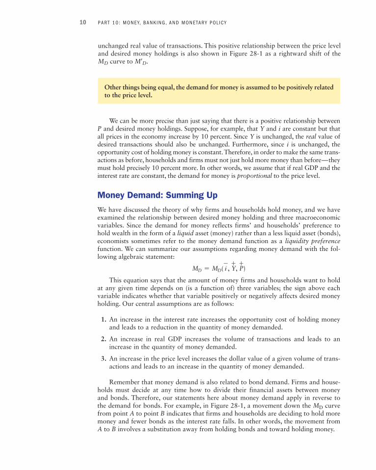
We can be more precise than just saying that there is a positive relationship between P and desired money holdings. Suppose, for example, that Y and i are constant but that all prices in the economy increase by 10 percent. Since Y is unchanged, the real value of desired transactions should also be unchanged. Furthermore, since i is unchanged, the opportunity cost of holding money is constant. Therefore, in order to make the same trans-actions as before, households and firms must not just hold more money than before—they must hold precisely 10 percent more. In other words, we assume that if real GDP and the interest rate are constant, the demand for money is proportional to the price level.
Money Demand: Summing Up
We have discussed the theory of why firms and households hold money, and we have examined the relationship between desired money holding and three macroeconomic variables. Since the demand for money reflects firms’ and households’ preference to hold wealth in the form of a liquid asset (money) rather than a less liquid asset (bonds), economists sometimes refer to the money demand function as a liquidity preference function. We can summarize our assumptions regarding money demand with the fol-lowing algebraic statement:
MD = MD( i-
, Y+
, P+
)
This equation says that the amount of money firms and households want to hold at any given time depends on (is a function of) three variables; the sign above each variable indicates whether that variable positively or negatively affects desired money holding. Our central assumptions are as follows:
1. An increase in the interest rate increases the opportunity cost of holding money and leads to a reduction in the quantity of money demanded.
2. An increase in real GDP increases the volume of transactions and leads to an increase in the quantity of money demanded.
3. An increase in the price level increases the dollar value of a given volume of trans-actions and leads to an increase in the quantity of money demanded.
Remember that money demand is also related to bond demand. Firms and house-holds must decide at any time how to divide their financial assets between money and bonds. Therefore, our statements here about money demand apply in reverse to the demand for bonds. For example, in Figure 28-1 , a movement down the M D curve from point A to point B indicates that firms and households are deciding to hold more money and fewer bonds as the interest rate falls. In other words, the movement from A to B involves a substitution away from holding bonds and toward holding money.
M28_RAGA8785_14_SE_C28.indd 10 04/10/12 12:49 PM
CHAPTER 28 : MONEY, I N TEREST RATES, AND ECONOMIC AC T I V I T Y 11
28.3 Monetary Equilibrium and National Income
So far, this chapter has been devoted to understanding bonds and how they relate to the demand for money. In the previous chapter we examined the supply of money. We are now ready to put these two sides of the money market together to develop a theory of how interest rates are determined in the short run. You may recall, however, that we already developed in Chapter 26 a theory of how interest rates are determined. But remember that Chapter 26 was a discussion of long-run economic growth, and real GDP was assumed to be equal to Y * throughout that discussion. What we do in this chapter and the next is return to the short-run version of our macro model but make it more complete by adding money and interest rates explicitly. We will see how changes in the money market can cause real GDP and interest rates to diverge for short periods of time from their long-run values.
We begin by examining the concept of monetary equilibrium— the theory of how interest rates are determined in the short run by the interaction of money demand and money supply. We then explore what economists call the monetary transmission mechanism— the chain of events that takes us from changes in the interest rate, through to changes in desired aggregate expenditure, to changes in the level of real GDP and the price level.
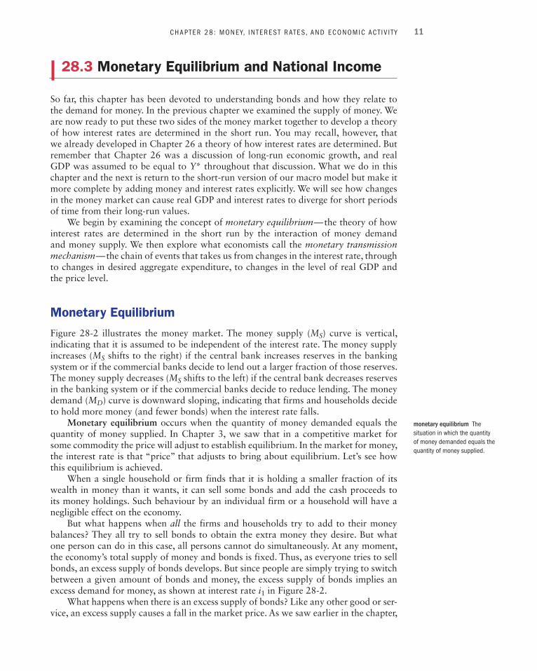
Monetary Equilibrium
Figure 28-2 illustrates the money market. The money supply ( M S ) curve is vertical, indicating that it is assumed to be independent of the interest rate. The money supply increases ( M S shifts to the right) if the central bank increases reserves in the banking system or if the commercial banks decide to lend out a larger fraction of those reserves. The money supply decreases ( M S shifts to the left) if the central bank decreases reserves in the banking system or if the commercial banks decide to reduce lending. The money demand ( M D ) curve is downward sloping, indicating that firms and households decide to hold more money (and fewer bonds) when the interest rate falls.
Monetary equilibrium occurs when the quantity of money demanded equals the quantity of money supplied. In Chapter 3 , we saw that in a competitive market for some commodity the price will adjust to establish equilibrium. In the market for money, the interest rate is that “price” that adjusts to bring about equilibrium. Let’s see how this equilibrium is achieved.
When a single household or firm finds that it is holding a smaller fraction of its wealth in money than it wants, it can sell some bonds and add the cash proceeds to its money holdings. Such behaviour by an individual firm or a household will have a negligible effect on the economy.
But what happens when all the firms and households try to add to their money balances? They all try to sell bonds to obtain the extra money they desire. But what one person can do in this case, all persons cannot do simultaneously. At any moment, the economy’s total supply of money and bonds is fixed. Thus, as everyone tries to sell bonds, an excess supply of bonds develops. But since people are simply trying to switch between a given amount of bonds and money, the excess supply of bonds implies an excess demand for money, as shown at interest rate i 1 in Figure 28-2 .
What happens when there is an excess supply of bonds? Like any other good or ser-vice, an excess supply causes a fall in the market price. As we saw earlier in the chapter,
monetary equilibrium The situation in which the quantity of money demanded equals the quantity of money supplied.
M28_RAGA8785_14_SE_C28.indd 11 04/10/12 12:49 PM

12 PART 10 : MONEY, BANK ING , AND MONETARY POL IC Y
a fall in the price of bonds implies an increase in the inter-est rate. As the interest rate rises, people economize on money balances because the opportunity cost of holding such balances is rising. Eventually, the interest rate will rise enough that people will no longer be trying to add to their money balances by selling bonds. At that point, there is no longer an excess supply of bonds (or an excess demand for money), and the interest rate will stop rising. The monetary equilibrium will have been achieved, as at point E in Figure 28-2 .
Suppose now there is more money than firms and households want to hold. That is, there is an excess sup-ply of money, as at interest rate i 2 in Figure 28-2 . The excess supply of money implies an excess demand for bonds—people are trying to “get rid of” their excess money balances by acquiring bonds. But when all house-holds try to buy bonds, they bid up the price of bonds, and the interest rate falls. As the interest rate falls, house-holds and firms become willing to hold larger quantities of money. The interest rate falls until firms and house-holds stop trying to convert bonds into money. In other words, it continues until everyone is content to hold the existing supply of money and bonds, as at point E in Figure 28-2 .
Monetary equilibrium occurs when the interest rate is such that the quantity of money demanded equals the quantity of money supplied.
The theory of interest-rate determination depicted in Figure 28-2 is often called the liquidity preference theory of interest. This name reflects the fact that when there are only two financial assets, a demand to hold money (rather than bonds) is a demand for the more liquid of the two assets—a preference for liquidity. The theory determines how the interest rate fluctuates in the short term as people seek to achieve portfolio balance, given fixed supplies of both money and bonds.
The Monetary Transmission Mechanism
The connection between changes in the demand for and supply of money and the level of aggregate demand is called the monetary transmission mechanism . It operates in three stages:
1. Changes in the demand for money or the supply of money cause a change in the equilibrium interest rate in the short run.
FIGURE 28-2 Monetary Equilibrium
The interest rate rises when there is an excess demand for money and falls when there is an excess supply of money. The fixed quantity of money M 0 is shown by the vertical supply curve M S . The money supply is determined by the behav-iour of the central bank as well as the commercial banks (as we saw in Chapter 27 ) . The demand for money is given by M D ; its negative slope indicates that a fall in the rate of interest causes the quantity of money demanded to increase. Monetary equi-librium is at E, with a rate of interest of i 0 .
If the interest rate is i 1 , there will be an excess demand for money of M 0 M 1 . Bonds will be offered for sale in an attempt to increase money holdings. This will force the rate of interest up to i 0 (the price of bonds falls), at which point the quantity of money demanded is equal to the fixed available quantity of M 0 . If the interest rate is i 2 , there will be an excess supply of money M 2 M 0 . Bonds will be demanded in return for excess money balances. This will force the rate of interest down to i 0 (the price of bonds rises), at which point the quantity of money demanded is equal to the fixed supply of M 0 .
0Quantity of Money
Excess demandfor money:
interest rate rises
Excess supplyof money:
interest rate falls
In
tere
st R
ate
M2
i2
i0
M0
i1
M1
E
MS
MD
monetary transmission
mechanism The channels by which a change in the demand for or supply of money leads to a shift of the aggregate demand curve.
M28_RAGA8785_14_SE_C28.indd 12 04/10/12 12:49 PM

CHAPTER 28 : MONEY, I N TEREST RATES, AND ECONOMIC AC T I V I T Y 13
2. The change in the interest rate leads to a change in desired investment and con-sumption expenditure (and net exports in an open economy).
3. The change in desired aggregate expenditure leads to a shift in the AD curve and thus to short-run changes in real GDP and the price level.
Let’s examine these three stages in more detail.
1. Changes in the Interest Rate The interest rate will change if the equilibrium depicted in Figure 28-2 is disturbed by a change in either the supply of money or the demand for money. For example, as shown in part (i) of Figure 28-3 , we see the following sequence of events when there is an increase in the supply of money but no change in the money demand curve:
c money supply 1 excess supply of money at initial interest rate
1 firms and households buy bonds
1 cbond prices
1 Tequilibrium interest rate
Note that the original increase in the supply of money could be caused either by the central bank increasing the reserves in the banking system or by the commercial banks lending out a higher fraction of their existing reserves.
FIGURE 28-3 Changes in the Equilibrium Interest Rate
Changes in the supply of money or in the demand for money cause the equilibrium interest rate to change. In both parts of the figure, the money supply is shown by the vertical curve M S , and the demand for money is shown by the negatively sloped curve M D . The initial monetary equilibrium is at E 0 , with corresponding interest rate i 0 . In part (i), an increase in the money supply causes M S
0 to shift to M S 1 . The new equilibrium is at E 1 , where the equilibrium interest
rate has fallen to i 1 . In part (ii), an increase in the demand for money shifts M D 0 to M D 1 . The new monetary equilibrium occurs at E 2 , and the equilibrium interest rate increases to i 2 .
0
Quantity of Money
Inte
rest
Rat
e
M0 M1
i1
i0
(i) An increase in the supply of money
E1
MD
MSMS
An increase inthe money supply reduces the equilibriuminterest rate
An increase inthe demand formoney increasesthe equilibriuminterest rate
0
Quantity of Money
Inte
rest
Rat
e
M0
i0
i2
(ii) An increase in the demand for money
E0
E2
MS
E0
0 1
MD
MD0
1
M28_RAGA8785_14_SE_C28.indd 13 04/10/12 12:50 PM

14 PART 10 : MONEY, BANK ING , AND MONETARY POL IC Y
As shown in part (ii) of Figure 28-3 , an increase in the demand for money, with an unchanged supply of money, leads to the following sequence of events:
c money supply 1 excess demand for money at initial interest rate
1 firms and households sell bonds
1 Tbond prices
1 cequilibrium interest rate
The original increase in the demand for money could be caused by an increase in real GDP or by an increase in the price level. It could also be caused by an increased prefer-ence to hold money rather than bonds, as would happen if there were an increase in the perceived riskiness of bonds.
Changes in either the demand for or the supply of money cause changes in the short-run equilibrium interest rate.
2. Changes in Desired Investment and Consumption The second link in the monetary transmission mechanism relates interest rates to desired investment and consumption expenditure. We saw in Chapter 21 that desired investment, which includes expendi-ture on inventory accumulation, residential construction, and business fixed invest-ment, responds to changes in the interest rate. Other things being equal, a decrease in the interest rate reduces the opportunity cost of borrowing or using retained earnings for investment purposes. As a result, the lower interest rate leads to an increase in desired investment expenditure. We also saw that consumption expenditures, especially on big-ticket durable items such as cars and furniture, which are often purchased on credit, are negatively related to the interest rate. In Figure 28-4 , this negative relationship between
FIGURE 28-4 The Effects of Changes in the Money Supply on Desired Investment Expenditure
Increases in the money supply reduce the equilibrium interest rate and increase desired investment expenditure . In part (i), monetary equilibrium is at E 0 , with a quantity of money of M 0 and an interest rate of i 0 . The corresponding level of desired investment is I 0 (point A ) in part (ii). An increase in the money supply to M 1 reduces the equilibrium interest rate to i 1 and increases investment expenditure by Δ I to I 1 (point B ).
0
Quantity of Money
Inte
rest
Rat
e
M0 M1
i1
i0
(i) Money demand and supply
E0
ID
E1
MD
0
Desired Investment Expenditure
Inte
rest
Rat
e
i1
i0
(ii) Investment demand
A
B
I0 I1
ΔI
MSMS0 1
M28_RAGA8785_14_SE_C28.indd 14 04/10/12 12:50 PM

CHAPTER 28 : MONEY, I N TEREST RATES, AND ECONOMIC AC T I V I T Y 15
4 In part (i) of Figure 28-4 , it is the nominal interest rate—the rate of return on bonds—that affects money demand. In part (ii), however, it is the real interest rate that influences desired investment expenditure. It is therefore worth emphasizing that we are continuing with the assumption that inflation is expected to be zero, and thus the nominal and real interest rates are the same. This assumption allows us to use the same vertical axis in the two parts of the figure.
An increase in the money supply causes a reduction in the interest rate and an increase in desired investment and other interest-sensitive expenditure; it therefore causes a rightward shift of the AD curve. A decrease in the money supply causes an increase in the interest rate and a decrease in desired investment; it therefore causes a leftward shift of the AD curve.
desired expenditure and the interest rate is labelled I D for investment demand, reflect-ing the fact that investment is the most interest-sensitive part of expenditure.
The first two links in the monetary transmission mechanism are shown in Figure 28-4 . 4
Although the analysis in Figure 28-4 illustrates a change in the money supply, remember that the transmission mechanism can also be set in motion by a change in the demand for money. In part (i), we see that an increase in the money supply reduces the short-run equilibrium interest rate. In part (ii), we see that a fall in the interest rate leads to an increase in desired investment (and consumption) expenditure.
3. Changes in Aggregate Demand The third link in our theory of the monetary trans-mission mechanism is from changes in desired expenditure to shifts in the AE function and in the AD curve. This is familiar ground. In Chapter 23 , we saw that a shift in the aggregate expenditure curve (caused by something other than a change in the price level) leads to a shift in the AD curve. This situation is shown again in Figure 28-5 .
FIGURE 28-5 The Effects of Changes in the Money Supply on Aggregate Demand
Changes in the money supply cause shifts in the AE and AD functions. In Figure 28-4 , an increase in the money supply increased desired investment expenditure by Δ I. In part (i) of this figure, the AE function shifts up by Δ I . At the fixed price level P 0 , equilibrium GDP rises from Y 0 to Y 1 , as shown by the rightward shift in the AD curve in part (ii).
Real GDP Real GDP
Des
ired
Agg
rega
te E
xpen
ditu
re
Pric
e L
evel
0
AE = Y
E1
(i) A shift in the AE curve
Y0
AE1(P0)
AE0(P0)
E0
Y1
P0
0
E1
(ii) A shift in the AD curve
Y0
AD1
Y1
ΔI
AD0
45°
E0
M28_RAGA8785_14_SE_C28.indd 15 04/10/12 12:50 PM
16 PART 10 : MONEY, BANK ING , AND MONETARY POL IC Y
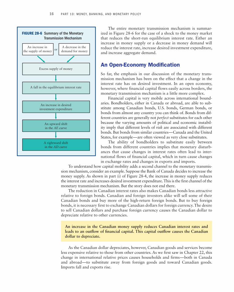
The entire monetary transmission mechanism is summar-ized in Figure 28-6 for the case of a shock to the money market that reduces the short-run equilibrium interest rate. Either an increase in money supply or a decrease in money demand will reduce the interest rate, increase desired investment expenditure, and increase aggregate demand.
An Open-Economy Modification
So far, the emphasis in our discussion of the monetary trans-mission mechanism has been on the effect that a change in the interest rate has on desired investment. In an open economy, however, where financial capital flows easily across borders, the monetary transmission mechanism is a little more complex.
Financial capital is very mobile across international bound-aries. Bondholders, either in Canada or abroad, are able to sub-stitute among Canadian bonds, U.S. bonds, German bonds, or bonds from almost any country you can think of. Bonds from dif-ferent countries are generally not perfect substitutes for each other because the varying amounts of political and economic instabil-ity imply that different levels of risk are associated with different bonds. But bonds from similar countries—Canada and the United States, for example—are often viewed as very close substitutes.
The ability of bondholders to substitute easily between bonds from different countries implies that monetary disturb-ances that cause changes in interest rates often lead to inter-national flows of financial capital, which in turn cause changes in exchange rates and changes in exports and imports.
To understand how capital mobility adds a second channel to the monetary transmis-sion mechanism, consider an example. Suppose the Bank of Canada decides to increase the money supply. As shown in part (i) of Figure 28-4 , the increase in money supply reduces the interest rate and increases desired investment expenditure. This is the first channel of the monetary transmission mechanism. But the story does not end there.
The reduction in Canadian interest rates also makes Canadian bonds less attractive relative to foreign bonds. Canadian and foreign investors alike will sell some of their Canadian bonds and buy more of the high-return foreign bonds. But to buy foreign bonds, it is necessary first to exchange Canadian dollars for foreign currency. The desire to sell Canadian dollars and purchase foreign currency causes the Canadian dollar to depreciate relative to other currencies.
FIGURE 28-6 Summary of the Monetary
Transmission Mechanism
An increase in the supply of money
A decrease in the demand for money
A rightward shiftin the AD curve
Excess supply of money
or
A fall in the equilibrium interest rate
An increase in desiredinvestment expenditure
An upward shiftin the AE curve
An increase in the Canadian money supply reduces Canadian interest rates and leads to an outfl ow of fi nancial capital. This capital outfl ow causes the Canadian dollar to depreciate.
As the Canadian dollar depreciates, however, Canadian goods and services become less expensive relative to those from other countries. As we first saw in Chapter 22 , this change in international relative prices causes households and firms—both in Canada and abroad—to substitute away from foreign goods and toward Canadian goods. Imports fall and exports rise.
M28_RAGA8785_14_SE_C28.indd 16 04/10/12 12:50 PM

CHAPTER 28 : MONEY, I N TEREST RATES, AND ECONOMIC AC T I V I T Y 17
So the overall effect of the increase in the Canadian money supply is not just a fall in Canadian interest rates and an increase in investment. Because of the international mobility of financial capital, the low Canadian interest rates also lead to a capital outflow, a depreciation of the Canadian dollar, and an increase in Canadian net exports. This increase in net exports, of course, strengthens the positive effect on aggregate demand already coming from the increase in desired investment.
This complete open-economy monetary transmission mechanism is shown in Figure 28-7 . This figure is based on Figure 28-6 , but simply adds the second channel of the transmission mechanism that works through capital mobility, exchange rates, and net exports.
In an open economy with capital mobility, an increase in the money supply is predicted to cause an increase in aggregate demand for two reasons. First, the reduc-tion in interest rates causes an increase in investment. Second, the lower interest rate causes a capital outfl ow, a currency depreciation, and a rise in net exports.
Our example has been that of a monetary expansion. A monetary contraction has the opposite effect, but the logic of the mechanism is the same. A reduction in the Canadian money supply raises Canadian interest rates and reduces desired investment expenditure. The higher Canadian inter-est rates attract foreign financial capital as bondholders sell low-return foreign bonds and purchase high-return Canadian bonds. This action increases the demand for Canadian dol-lars in the foreign-exchange market and thus causes the Canadian dollar to appreciate. Finally, the appreciation of the Canadian dollar increases Canadians’ imports of foreign goods and reduces Canadian exports to other countries. Canadian net exports fall.
The Slope of the AD Curve
We can now use our theory of the monetary transmission mechanism to add to the explanation of the negative slope of the AD curve. In Chapter 23 , we mentioned two reasons for its negative slope: the change in wealth and the substitution between domes-tic and foreign goods, both of which occur when the domestic price level changes. A third effect operates through interest rates, and works as follows. A rise in the price level raises the money value of transactions and thus leads to an increase in the demand for money. For a given supply of money (a vertical M S curve), the increase in money demand means that the M D curve shifts to the right, raising the equilibrium interest rate. The higher interest rate then leads to a reduction in desired investment expenditure. We therefore have a third reason that the price level and the level of aggregate demand are negatively related. This third reason for the negative slope of the AD curve is import-ant because, empirically, the interest rate is the most important link between monetary factors and real expenditure flows.
FIGURE 28-7 The Open-Economy Monetary
Transmission Mechanism
Capital outflow andcurrency depreciation
Excess supply of money
Upward shiftin AE curve
Rightward shift of AD curve
Fall in the equilibrium interest rate
or
Increase in desiredinvestment expenditure
Decrease indemand for money
Increase insupply of money
Increase innet exports
M28_RAGA8785_14_SE_C28.indd 17 04/10/12 12:50 PM
18 PART 10 : MONEY, BANK ING , AND MONETARY POL IC Y
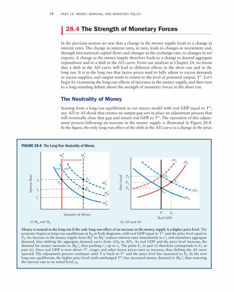
FIGURE 28-8 The Long-Run Neutrality of Money
Money is neutral in the long run if the only long-run effect of an increase in the money supply is a higher price level. The economy begins in long-run equilibrium at E 0 in both diagrams, with real GDP equal to Y * and the price level equal to P 0 . An increase in the money supply from M S
0 to M S 1 reduces interest rates immediately to i œ 1 and stimulates aggregate
demand, thus shifting the aggregate demand curve from AD 0 to AD 1 . As real GDP and the price level increase, the demand for money increases to M D 1 , thus pushing i œ 1 up to i 1 . The point E 1 in part (i) therefore corresponds to E 1 in part (ii). Since real GDP is now above Y *, wages and other factor prices start to increase, thus shifting the AS curve upward. The adjustment process continues until Y is back to Y * and the price level has increased to P 2 . In the new long-run equilibrium, the higher price level (with unchanged Y *) has increased money demand to M D 2 , thus restoring the interest rate to its initial level, i 0 .
•
••
•
•
••
MD
MD0
1
MD2
MS0
MS1
P2
Y1
Real GDP(ii) AD and AS
Pric
e L
evel E2
Y∗
E0
P0
P1
AD1
AD0
AS1 AS0
E1i0
Quantity of Money
(i) MD and MS
Inte
resr
Rat
e
i1'
i1E1
E2E0
28.4 The Strength of Monetary Forces
In the previous section we saw that a change in the money supply leads to a change in interest rates. The change in interest rates, in turn, leads to changes in investment and, through international capital flows and changes in the exchange rate, to changes in net exports. A change in the money supply therefore leads to a change in desired aggregate expenditure and to a shift in the AD curve. From our analysis in Chapter 24 , we know that a shift in the AD curve will lead to different effects in the short run and in the long run. It is in the long run that factor prices tend to fully adjust to excess demands or excess supplies, and output tends to return to the level of potential output, Y *. Let’s begin by examining the long-run effects of increases in the money supply, and then turn to a long-standing debate about the strength of monetary forces in the short run.
The Neutrality of Money
Starting from a long-run equilibrium in our macro model with real GDP equal to Y *, any AD or AS shock that creates an output gap sets in place an adjustment process that will eventually close that gap and return real GDP to Y *. The operation of this adjust-ment process following an increase in the money supply is illustrated in Figure 28-8 . In the figure, the only long-run effect of the shift in the AD curve is a change in the price
M28_RAGA8785_14_SE_C28.indd 18 04/10/12 12:50 PM

CHAPTER 28 : MONEY, I N TEREST RATES, AND ECONOMIC AC T I V I T Y 19
level; there is no long-run effect on real GDP or any other real economic variable. This result is referred to as long-run money neutrality . The long-run neutrality of money requires that Y * be unaffected by changes in the supply of money.
The Classical Dichotomy Many eighteenth and nineteenth century economists developed theories of the economy’s long-run equilibrium and emphasized the neutrality of money. They argued that the “monetary side” of the economy was independent from the “real side” in the long run. This belief came to be referred to as the Classical Dichot-omy . In the long run, relative prices, real GDP, employment, investment, and all other real economic variables were assumed to be determined by real factors, such as firms’ technologies and consumers’ preferences. The absolute level of money prices was then determined by the monetary side of the economy, where the quantity of money deter-mined the price level. In macro models that contain this dichotomy, the long-run effect of a change in the money supply is a change in the price level, with no changes to any real economic variables.
The concept of money neutrality is interpreted differently by different people. Our definition above, which emphasizes the independence of Y * from the country’s money supply, is probably the most commonly used definition today, but there are others as well. Applying Economic Concepts 28-2 examines the concept of money neutrality as it relates to changes in the denominations of a country’s paper currency.
long-run money neutrality The idea that a change in the supply of money has no long-run effect on any real variables; it only affects the price level.
APPLYING ECONOMIC CONCEPTS 28-2
Monetary Reform and the Neutrality of Money
The least controversial proposition regarding the neu-trality of money is that altering the number of zeros on the monetary unit, and on everything else stated in those units, will have no economic consequences. For example, if an extra zero were added to all Bank of Canada notes—so that all $5 bills became $50 bills, all $10 bills became $100 bills, and so on—and the same adjustment was made to all nominal wages, prices, and contracts in the economy, there would be no effects on real GDP, real wages, relative prices, and other real economic variables.*
This proposition has been tested many times since the Second World War, when countries that had suf-fered major inflations undertook monetary reform by reducing the number of zeros on the monetary unit and everything else that was specified in money terms. The evidence is clear that no significant or lasting effects fol-lowed from these reforms. That such money neutrality is a testable theory, rather than merely a definitional statement, is shown by the observable possibility that for a short time after the monetary reforms some people may be so ill informed, and others such creatures of habit, that they make mistakes based on assuming that the new money is the same as the old. Although some
such behaviour probably occurred, it was not signifi-cant enough to show up as a sudden change in any of the economic data that have been collected in these cases.
A slightly stronger proposition regarding money neutrality is that altering the nature of the monetary unit will have no real economic effects. Such a change occurred, for example, in 1971, when the United Kingdom changed from a system in which the basic monetary unit, the pound sterling, was composed of 240 pence to a system in which it contained 100 pence. Another example is Ireland’s 1999 conversion from the punt, which contained 240 pence, to the euro, which contained 100 cents. In these cases there were some alterations in real behaviour immediately after the change was made, as many people were confused by the new units. Once again, however, these changes were neither import-ant enough nor long-lasting enough to show up in the macroeconomic data.
These two propositions regarding the neutrality of money are important because they emphasize the nominal nature of money, and the important distinction between nominal and real values. It would be unusual indeed if multiplying all nominal values in the economy
(continued)
M28_RAGA8785_14_SE_C28.indd 19 04/10/12 12:50 PM

20 PART 10 : MONEY, BANK ING , AND MONETARY POL IC Y
Hysteresis Effects The proposition of long-run money neutrality is debatable. Though it is a common assumption in many macroeconomic models, there are good reasons to think that changes in a country’s money supply may have effects on Y* and thus have long-run effects on real GDP. Here we examine what is called hysteresis —the possibility that the level or growth rate of Y* may be affected by the short-run path of real GDP.
Investment and Technology. Theories that assume long-run money neutrality typically omit some key economic behaviour that blurs the division between the real and monetary sectors of the economy. Credit plays a key role in linking these two sectors. Most firms use credit to finance aspects of their regular operations as well as their investments in research and development and the expansion of their production facilities. In short, credit can be viewed as an important input to firms’ production and investment activities.
Now consider the effects of a change in the country’s money supply. As we have seen in this chapter, the likely short-run effects are changes in interest rates and the level of real GDP. But if the change in firms’ access to credit—associated with the change in interest rates—also leads firms to alter their capital investment and expenditures on research and development, there may be a permanent effect on the economy’s capital stock and state of technology. If so, there will be a permanent effect on the level of potential output.
A dramatic example of the important role of credit occurred with the global finan-cial crisis that began in 2008. As several large U.S. and European banks failed, the flows of credit to non-financial firms dropped sharply in many countries. The reduced access to credit led to reductions in investment, employment, and output, and contributed to the largest global recession in over half a century.
Money is neutral in the long run if a change in the money supply has no long-run effect on real GDP or any other real variables. Many modern economists believe that empirical evidence is consistent with long-run money neutrality, although the proposition is often debated.
FPO
dummy captions, dummy captions, dummy captions, dummy captions, dummy captions, dummy captions, dummy captions, dummy captions, dummy captions
by the same scalar had any real effect other than some temporary confusion. For this reason, these two propos-itions are accepted by virtually all economists and central bankers.
The stronger and more controversial proposition regarding money neutrality is the one discussed in the text — that the economy’s level of potential output is unaffected by changes in the supply of money. This assumption is common in many macroeconomic models but, as we argue in the text, there are good reasons to think that monetary policy may have effects on Y* and thus have long-run effects on real GDP.
*Of course, there would be some real effects from such an adjustment, including the level of inconvenience associated with using paper money with larger denominations (which would be enormous if we added many zeros rather than just one to all existing bills and prices).
APPLYING ECONOMIC CONCEPTS 28-2 (continued)
M28_RAGA8785_14_SE_C28.indd 20 04/10/12 12:50 PM

CHAPTER 28 : MONEY, I N TEREST RATES, AND ECONOMIC AC T I V I T Y 21
Long-run money neutrality is called into question by the possibility that a change in the money supply, through its effect on the interest rate, can affect the course of investment and technological change and hence the path of potential output.
Human Capital. Another reason for hysteresis is the effect on human capital that often ac-companies prolonged unemployment. Consider a negative shock that reduces real GDP and increases the unemployment rate. If wages and other factor prices are slow to adjust, some individuals will experience long spells of unemployment. Prolonged lack of work for even experienced workers may cause their skills to deteriorate. The effect can be even stronger with first entrants to the labour force. If young people are denied the experience of early jobs that teach them the disciplines and basic skills required of all members of the labour force, it may be difficult or even impossible for them to learn these skills later when jobs do become available. If the recession lasts long enough, both groups may eventually become “unemployable,” even after the aggregate economy recovers. In this case, the fall in the level of real GDP, if prolonged, leads through hysteresis effects to a fall in the level of Y* .
The major global recession that began in 2008 again provides an example to illustrate these effects. Even three years into a slow economic recovery, the amount of long-term unemployment among both experienced and young workers was higher in the United States than at any time in the recent past. In Europe, the situation was even worse, with long-term youth unemployment running from 20 to over 40 percent in the more depressed economies such as Greece and Spain. There is little doubt that the stock of productive human capital that will exist when these countries eventually return to something like full employment will be permanently below what it would have been if the prolonged recession had not occurred.
If a long period of unemployment associated with a prolonged recessionary gap causes workers to lose human capital, or accumulate less than they otherwise would, both the level and rate of growth of Y* may be reduced when the recession-ary gap is eventually closed.
Money and Inflation
Whether or not money is neutral in the long run, it is certainly closely related to the price level. As we observed in Chapter 27 (in Applying Economic Concepts 27-1 ), there have been many examples throughout history of countries experiencing dramatic increases in the money supply and equally dramatic increases in the price level.
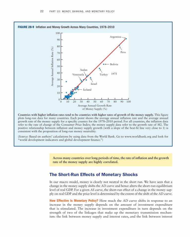
The close connection between money growth and inflation does not just hold in the dramatic examples; it is a connection that applies in the long run to most if not all econ-omies. Figure 28-9 shows a scatter plot of inflation and money growth for a large sample of countries between 1978 and 2010. The vertical axis measures each country’s average annual inflation rate. The horizontal axis measures each country’s average annual growth rate of the money supply. Each point in the figure represents the rates of inflation and money supply growth for one country averaged over the sample period. As is clear in the figure, there is a strong positive correlation between the growth rate of the money supply and the rate of inflation, as reflected by the tight bunching of points around the upward-sloping line. This line is the statistical “line of best fit” between money supply growth and inflation. Its slope is 0.97, indicating that two countries that differ in their money growth rates by 10 percent will, on average, differ in their inflation rates by 9.7 percent.
M28_RAGA8785_14_SE_C28.indd 21 04/10/12 12:50 PM
22 PART 10 : MONEY, BANK ING , AND MONETARY POL IC Y
FIGURE 28-9 Inflation and Money Growth Across Many Countries, 1978–2010
Countries with higher inflation rates tend to be countries with higher rates of growth of the money supply. This figure plots long-run data for many countries. Each point shows the average annual inflation rate and the average annual growth rate of the money supply for a specific country for the 1978–2010 period. For all countries, the inflation data refer to the rate of change of the Consumer Price Index; the money supply data refer to the growth rate of M 2. The positive relationship between inflation and money supply growth (with a slope of the best-fit line very close to 1) is consistent with the proposition of long-run money neutrality.
( Source: Based on authors’ calculations by using data from the World Bank. Go to www.worldbank.org and look for “world development indicators and global development finance.”)
Iceland
Israel
Sudan
Bolivia
Argentina
Venezuela Turkey
Peru
1975
00
10
20
30
40
50
60
70
80
90
100
10 20 30 40 50
Average Annual Growth Rateof Money Supply (%)
Ave
rage
Ann
ual I
nflat
ion
Rat
e (%
)
60 70 80 90 100
Across many countries over long periods of time, the rate of infl ation and the growth rate of the money supply are highly correlated.
The Short-Run Effects of Monetary Shocks
In our macro model, money is clearly not neutral in the short run. We have seen that a change in the money supply shifts the AD curve and hence alters the short-run equilibrium level of real GDP. For a given AS curve, the short-run effect of a change in the money sup-ply on real GDP and the price level is determined by the extent of the shift of the AD curve.
How Effective Is Monetary Policy? How much the AD curve shifts in response to an increase in the money supply depends on the amount of investment expenditure that is stimulated. The increase in investment expenditure in turn depends on the strength of two of the linkages that make up the monetary transmission mechan-ism: the link between money supply and interest rates, and the link between interest
M28_RAGA8785_14_SE_C28.indd 22 04/10/12 12:50 PM

CHAPTER 28 : MONEY, I N TEREST RATES, AND ECONOMIC AC T I V I T Y 23
rates and investment. 5 Let’s look more closely at these separate parts of the monetary transmission mechanism.
First, consider how much interest rates fall in response to an increase in the money supply. If the M D curve is steep, a given increase in the money supply will lead to a large reduction in the equilibrium interest rate. A steep M D curve means that firms’ and households’ desired money holding is not very sensitive to changes in the interest rate, so interest rates have to fall a lot to get people to be content to hold a larger amount of money. The flatter the M D curve, the less interest rates will fall for any given increase in the supply of money.
Second, consider how much investment expenditure increases in response to a fall in interest rates. If the I D curve is relatively flat, then any given reduction in interest rates will lead to a large increase in firms’ desired investment. The steeper the I D curve, the less investment will increase for any given reduction in interest rates.
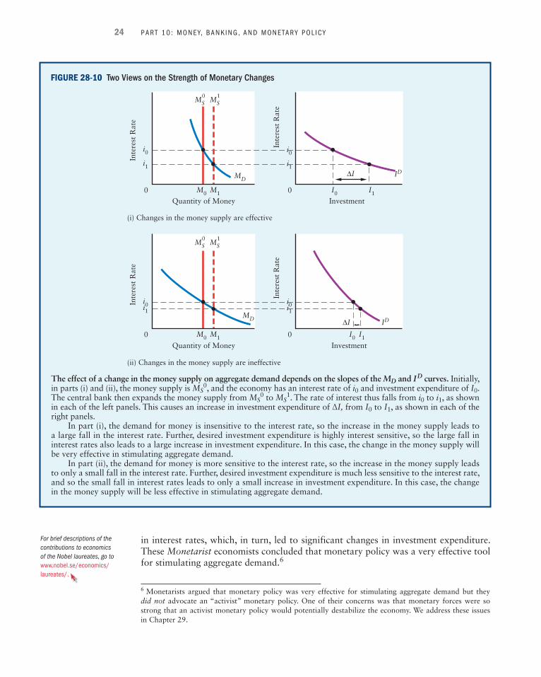
It follows that the size of the shift of the AD curve in response to a change in the money supply depends on the shapes of the M D and I D curves. The influence of the shapes of the two curves is shown in Figure 28-10 and can be summarized as follows:
1. The steeper the M D curve, the more interest rates will change in response to a given change in the money supply.
2. The flatter the I D curve, the more investment expenditure will change in response to a given change in the interest rate, and hence the larger the shift in the AD curve.
The combination that produces the largest shift in the AD curve for a given change in the money supply is a steep M D curve and a flat I D curve. This combination is illustrated in part (i) of Figure 28-10 . It makes monetary policy relatively effective as a means of influencing real GDP in the short run. The combination that produces the smallest shift in the AD curve is a flat M D curve and a steep I D curve. This combination is illustrated in part (ii) of Figure 28-10 . It makes monetary policy relatively ineffective in the short run.
5 As we saw earlier in the chapter, the consumption of durable goods is also sensitive to changes in the interest rate. In this section, however, we simplify by focusing only on the behaviour of desired investment.
The effectiveness of monetary policy in inducing short-run changes in real GDP depends on the slopes of the M D and I D curves. The steeper is the M D curve, and the fl atter is the I D curve, the more effective is monetary policy.
Keynesians versus Monetarists Figure 28-10 illustrates a famous debate among economists that occurred in the three decades following the Second World War. Some economists, following the ideas of John Maynard Keynes, argued that changes in the money supply led to relatively small changes in interest rates, and that investment was relatively insensitive to changes in the interest rate. These Keynesian economists concluded that monetary policy was not a very effective method of stimulating aggre-gate demand—they therefore emphasized the value of using fiscal policy (as Keynes himself had argued during the Great Depression). Another group of economists, led by Milton Friedman, argued that changes in the money supply caused sharp changes
M28_RAGA8785_14_SE_C28.indd 23 04/10/12 12:50 PM
24 PART 10 : MONEY, BANK ING , AND MONETARY POL IC Y
in interest rates, which, in turn, led to significant changes in investment expenditure. These Monetarist economists concluded that monetary policy was a very effective tool for stimulating aggregate demand. 6
FIGURE 28-10 Two Views on the Strength of Monetary Changes
The effect of a change in the money supply on aggregate demand depends on the slopes of the M D and I D curves. Initially, in parts (i) and (ii), the money supply is M S
0 , and the economy has an interest rate of i 0 and investment expenditure of I 0 . The central bank then expands the money supply from M S
0 to M S 1 . The rate of interest thus falls from i 0 to i 1 , as shown
in each of the left panels. This causes an increase in investment expenditure of Δ I, from I 0 to I 1 , as shown in each of the right panels.
In part (i), the demand for money is insensitive to the interest rate, so the increase in the money supply leads to a large fall in the interest rate. Further, desired investment expenditure is highly interest sensitive, so the large fall in interest rates also leads to a large increase in investment expenditure. In this case, the change in the money supply will be very effective in stimulating aggregate demand.
In part (ii), the demand for money is more sensitive to the interest rate, so the increase in the money supply leads to only a small fall in the interest rate. Further, desired investment expenditure is much less sensitive to the interest rate, and so the small fall in interest rates leads to only a small increase in investment expenditure. In this case, the change in the money supply will be less effective in stimulating aggregate demand.
•••
•
••
••
i1
i0
Quantity of Money
Inte
rest
Rat
e
0
(i) Changes in the money supply are effective
M1
i0
i1
Investment
Inte
rest
Rat
e
0 I0 I1
ID
ID
MD
MD
M0
ΔI
i1i0
Quantity of Money
Inte
rest
Rat
e
0
(ii) Changes in the money supply are ineffective
M1
i0i1
Investment
Inte
rest
Rat
e
0 I0 I1M0
ΔI
MSMS0 1
MSMS0 1
6 Monetarists argued that monetary policy was very effective for stimulating aggregate demand but they did not advocate an “activist” monetary policy. One of their concerns was that monetary forces were so strong that an activist monetary policy would potentially destabilize the economy. We address these issues in Chapter 29 .
For brief descriptions of the
contributions to economics
of the Nobel laureates, go to
www.nobel.se/economics/laureates/ .
M28_RAGA8785_14_SE_C28.indd 24 04/10/12 12:50 PM

CHAPTER 28 : MONEY, I N TEREST RATES, AND ECONOMIC AC T I V I T Y 25
Today, this debate between Keynesians and Monetarists is over. A great deal of empirical research suggests that money demand is relatively insensitive to changes in the interest rate. That is, the M D curve is quite steep and, as a result, changes in the money supply cause relatively large changes in interest rates (as argued by the Monetarists). The evidence is much less clear, however, on the slope of the I D curve. Though the evidence confirms that I D is downward sloping, there is no consensus on whether the curve is steep or flat. Part of the problem facing researchers is that an important determinant of investment is not observable. Firms’ expectations about the future—what Keynes famously called firms’ “animal spirits”—have a significant effect on their investment decisions (thus shifting the I D curve), but this variable is not easily measured by researchers. The non-observability of this variable makes it very difficult to estimate precisely the relationship between interest rates and invest-ment. Another problem is that the I D curve is an aggregation of a number of differ-ent investment demands (plant, equipment, inventories, new housing, and durable consumer goods), each subject to different influences. While each type of investment is responsive to changes in the interest rate, their individual differences make it dif-ficult to estimate the responsiveness of aggregate desired investment ( I D ) to changes in the interest rate.
Though empirical research over the years has largely filled the gaps in our knowledge, there is still plenty of debate about the effectiveness and the appropriate objectives of monetary policy. Some economists argue that monetary policy should be directed only to achieving a desired path of the price level, with little or no atten-tion being paid to fluctuations in real GDP. Others argue that monetary policy should attempt to offset the largest and most persistent shocks that hit the economy, while maintaining a long-run focus on the behaviour of the price level. Yet others argue that short-run fluctuations in real GDP and employment are so important that monetary policy ought to place much less emphasis on the price level and instead be actively engaged in reducing the economy’s fluctuations in the face of all but the smallest and most transient shocks.
In the next chapter we examine the details of how monetary policy is conducted in Canada. For several reasons, the real-world practice of monetary policy is more com-plex than it appears in this chapter. But as we will see, the Bank of Canada’s system of inflation targeting can be viewed as a means of providing both short-run stabilization and a long-run focus on the behaviour of the price level.
SUMMARY
28.1 Understanding Bonds LO 1
• The present value of any bond that promises to pay some sequence of payments in the future is negatively related to the market interest rate. A bond’s present value determines its market price. Thus, there is a nega-tive relationship between the market interest rate and the price of a bond.
• The yield on a bond is the rate of return the bondholder receives, having bought the bond at its
purchase price and then receiving the entire stream of future payments the bond offers. For a given stream of future payments, a lower purchase price implies a higher bond yield.
• An increase in the perceived riskiness of bonds leads to a reduction in bond prices and thus an increase in bond yields.
M28_RAGA8785_14_SE_C28.indd 25 04/10/12 12:50 PM

26 PART 10 : MONEY, BANK ING , AND MONETARY POL IC Y
28.4 The Strength of Monetary Forces LO 5, 6
28.3 Monetary Equilibrium and National Income LO 3, 4
• Changes in the money supply have different effects on the economy in the short run and in the long run.
• Money is said to be neutral in the long run if a change in the money supply leads to no changes in the long-run level of real GDP (or other real variables).
• In the long run, after wages and other factor prices have fully adjusted to any output gaps, real GDP returns to potential output, Y *. If Y* is unaffected by the change in the money supply, there will be no long-run effect from the monetary shock.
• If there is hysteresis, short-run changes in real GDP will lead to changes in Y* . In these cases, monetary shocks will have long-run effects on real GDP.
• In the short run, the interest rate is determined by the interaction of money supply and money demand. Mon-etary equilibrium is established when the interest rate is such that the quantity of money supplied is equal to the quantity of money demanded.
• A change in the money supply (coming from the cen-tral bank or the commercial banking system) or in the demand for money (coming from a change in Y or P ) will lead to a change in the equilibrium interest rate. This is the first stage of the monetary transmission mechanism.
• There is a strong positive correlation between the rate of money growth and the rate of inflation across coun-tries when viewed over the long run.
• In the short run, the effects of a change in the money supply depend on the shape of the M D and I D curves in our macro model. The steeper the M D curve and the flatter the I D curve, the more effective changes in the money supply will be in causing short-run changes in real GDP.
• The second stage of the monetary transmission mech-anism is that any change in the interest rate leads to a change in desired investment and consumption expendi-ture. In an open economy with capital mobility, the change in the interest rate leads to capital flows, chan-ges in the exchange rate, and changes in net exports.
• The third stage of the monetary transmission mechan-ism is that any change in desired investment, consump-tion, or net exports leads to a shift in the aggregate demand ( AD ) curve, and thus to a change in real GDP and the price level.
The interest rate and present value Interest rates, bond prices, and bond yields Reasons for holding money The money demand ( M D ) function
Monetary equilibrium The monetary transmission mechanism The investment demand ( I D ) function
Effects of changes in the money supply Neutrality and non-neutrality of money Hysteresis
KEY CONCEPTS
28.2 The Theory of Money Demand LO 2
• In our macro model, households and firms are assumed to divide their financial assets between interest-bearing “bonds” and non–interest-bearing “money.” They hold money to facilitate both expected and unexpected trans-actions, and also to protect against the possibility of a decline in bond prices (a rise in interest rates).
• The opportunity cost of holding money is the interest that would have been earned if bonds had been held instead.
• Households’ and firms’ desired money holdings are assumed to be influenced by three key macroeconomic variables: 1. Increases in the interest rate reduce desired money
holdings.
2. Increases in real GDP increase desired money holdings. 3. Increases in the price level increase desired money
holdings. • These relationships are captured in the M D curve, which
is drawn as a negative relationship between interest rates ( i ) and desired money holding ( M D ). Increases in real GDP ( Y ) or the price level ( P ) lead to a rightward shift of this M D curve.
M28_RAGA8785_14_SE_C28.indd 26 04/10/12 12:50 PM

CHAPTER 28 : MONEY, I N TEREST RATES, AND ECONOMIC AC T I V I T Y 27
1. Fill in the blanks to make the following statements cor-rectly reflect the theory developed in this chapter.
a. Monetary equilibrium occurs when the quantity of ________ equals the quantity of ________. Monetary equilibrium determines the ________.
b. When there is an excess supply of money, house-holds and firms will attempt to ________ bonds. This action will cause the price of bonds to ________ and the interest rate to ________.
c. When there is an excess demand for money, house-holds and firms will attempt to ________ bonds. This action will cause the price of bonds to ________ and the interest rate to ________.
d. The ________ ________ ________ refers to the three stages that link the money market to aggregate demand. The first link is between monetary equilib-rium and the ________; the second link is between the ________ and desired ________; the third link is between desired ________ and ________.
e. Suppose the economy is in equilibrium and then the Bank of Canada increases the money supply. The first effect will be an excess ________ of/for money, which will then lead to a ________ in the interest rate, which will in turn lead to a(n) ________ in desired investment.
f. Suppose the economy is in equilibrium and the Bank of Canada decreases the money supply. The first effect will be an excess ________ of/for money, which will lead to a ________ in the interest rate, which will in turn lead to a(n) ________ in desired investment.
g. Through the monetary transmission mechanism, a rightward shift of the AD curve can be caused by a(n) ________ in the money supply; a leftward shift of the AD curve can be caused by a(n) ________ in the money supply.
h. In an open economy with capital mobility, an increase in the money supply causes interest rates to ________, which leads to a capital outflow. This causes a(n) ________ of the Canadian dollar and thus to a(n) ________ in net exports, which leads the AD curve to shift ________.
2. Fill in the blanks to make the following statements cor-rectly reflect the theory developed in this chapter.
a. If money is neutral in the long run, then changes in the money supply have no effect on _______ in the long run.
b. If the demand for money is not very sensitive to changes in the interest rate, then the M D curve will be relatively ________. An increase in the money supply will lead to a ________ reduction in the interest rate.
c. If the demand for money is very sensitive to chan-ges in the interest rate, then the M D curve will be relatively ________. An increase in the money supply will lead to a ________ reduction in the interest rate.
d. A relatively flat investment demand curve means that a change in the interest rate will have a ________ effect on ________, which leads to a rela-tively large shift in the ________ curve.
e. A relatively steep investment demand curve means that a change in the interest rate will have a ________ effect on ________, which leads to a rela-tively small shift in the ________ curve.
f. Changes in the money supply will have the largest effect on the position of the AD curve when the M Dcurve is ________ and the I D curve is ________.
3. The following table shows the stream of income pro-duced by several different assets. In each case, P 1 , P 2 , and P 3 are the payments made by the asset in Years 1, 2, and 3.
Asset
Market Interest Rate ( i ) P 1 P 2 P 3
Present Value
Treasury Bill
4% $1000 $0 $0 —
Bond 3% $0 $0 $5000 —
Bond 5% $200 $200 $200 —
Stock 6% $50 $40 $60 —
STUDY EXERCISES
Make the grade with MyEconLab: Study Exercises marked in red can be found on MyEconLab. You can practise them as often as you want, and most feature step-by-step guided instructions to help you find the right answer.
MyEconLab
M28_RAGA8785_14_SE_C28.indd 27 04/10/12 12:50 PM

28 PART 10 : MONEY, BANK ING , AND MONETARY POL IC Y
a. For each asset, compute the asset’s present value. (Note that the market interest rate, i, is not the same in each situation.)
b. Explain why the market price for each asset will be the asset’s present value.
4. The table below provides information for six differ-ent bonds: current market price ( P ), the face value of the bond ( V ), and the number of years before the bond matures ( N ).
Bond Number
Market Price ( P )
Face Value ( V )
Years to Maturity ( N )
1a $926 $1000 1
1b $850 $1000 1
2a $1270 $2000 5
2b $838 $2000 5
3a $1760 $5000 10
3b $684 $5000 10
a. In each case, compute the bond’s yield, assuming that you buy the bond at its current market price and hold the bond until it matures. There are no coupons. If x is the bond’s yield, then P (1 + x ) N = V .
b. Suppose bonds 1a, 2a, and 3a are all issued by the same borrower. Can you offer an explanation for the relationship between the bond yields and the terms to maturity?
c. Suppose bonds 1b, 2b, and 3b are all issued by the same borrower. What can you conclude about the riskiness of the “a” borrower versus that of the “b” borrower? Explain.
d. Notice that the market interest rate is not shown in the table. Explain why knowledge of the market interest rate is unnecessary in order to compute a bond’s yield, once you already know the bond’s market price. What aspect of the bond does the market interest rate influence, if anything?
5. Imagine a bond that promises to make coupon pay-ments of $100 one year from now and $100 two years from now, and to repay the principal of $1000 three years from now. Suppose also that the market interest rate is 8 percent per year, and that no perceived risk is associated with the bond.
a. Compute the present value of this bond. b. Suppose the bond is being offered for $995. Would
you buy the bond at that price? What do you expect to happen to the bond price in the very near future?
c. Suppose the bond is instead being offered at a price of $950. Would you buy the bond at that price? Do you expect the bond price to change in the near future?
d. If the price of the bond is equal to its computed present value from part (a), what is the implied bond yield?
e. Explain why bond yields and the market interest rate tend to move together so that economists can then sensibly speak about “the” interest rate.
6. What motives for holding money—transactions, pre-cautionary, or speculative—do you think explain the following holdings? Explain.
a. Currency in the cash register of the local grocery store at the start of each working day.
b. Money to meet Queen’s University’s biweekly pay-roll deposited in the local bank.
c. A household tries to keep a “buffer” of $1000 in its savings account.
d. An investor sells bonds for cash, which she then deposits in a low-return bank account.
e. You carry $20 in your pocket even though you have no planned expenditures.
7. The diagram below shows the demand for money and the supply of money.
i*
Quantity of Money
Inte
rest
Rat
e
0
MD (Y, P)
MS
iB
iA
a. Explain why the M D function is downward sloping. b. Suppose the interest rate is at i A . Explain how
firms and households attempt to satisfy their excess demand for money. What is the effect of their actions?
c. Suppose the interest rate is at i B . Explain how firms and households attempt to dispose of their excess supply of money. What is the effect of their actions?
d. Now suppose there is an increase in the transactions demand for money (perhaps because of growth in real GDP). Beginning at i *, explain what happens in the money market. How is this shown in the diagram?
8. The following diagrams show the determination of monetary equilibrium and the demand for investment. The economy begins with money supply M S , money demand M D , and investment demand I D . The interest rate is i 0 and desired investment is I 0 .
M28_RAGA8785_14_SE_C28.indd 28 04/10/12 12:50 PM
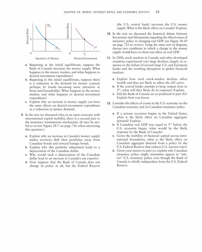
CHAPTER 28 : MONEY, I N TEREST RATES, AND ECONOMIC AC T I V I T Y 29
Inte
rest
Rat
eMS
MD ID
Inte
rest
Rat
e
I0
Desired Investment
00
i0
Quantity of Money
a. Beginning at the initial equilibrium, suppose the Bank of Canada increases the money supply. What happens in the money market, and what happens to desired investment expenditure?
b. Beginning in the initial equilibrium, suppose there is a reduction in the demand for money (caused, perhaps, by bonds becoming more attractive to firms and households). What happens in the money market, and what happens to desired investment expenditure?
c. Explain why an increase in money supply can have the same effects on desired investment expenditure as a reduction in money demand.
9. In the text we discussed why, in an open economy with international capital mobility, there is a second part to the monetary transmission mechanism. (It may be use-ful to review Figure 28-7 on page 716 when answering this question.)
a. Explain why an increase in Canada’s money supply makes investors shift their portfolios away from Canadian bonds and toward foreign bonds.
b. Explain why this portfolio adjustment leads to a depreciation of the Canadian dollar.
c. Why would such a depreciation of the Canadian dollar lead to an increase in Canada’s net exports?
d. Now suppose that the Bank of Canada does not change its policy at all, but the Federal Reserve
(the U.S. central bank) increases the U.S. money supply. What is the likely effect on Canada? Explain.
10. In the text we discussed the historical debate between Keynesians and Monetarists regarding the effectiveness of monetary policy in changing real GDP (see Figure 28-10 on page 721 to review). Using the same sort of diagram, discuss two conditions in which a change in the money supply would have no short-run effect on real GDP.
11. In 2008, stock markets in Canada and other developed countries experienced very large declines, largely in re-sponse to the failure of several large U.S. and European banks and the resulting disruption in global financial markets.
a. Explain how such stock-market declines affect wealth and thus are likely to affect the AD curve.
b. If the central banks attempt to keep output close to Y *, what will they likely do in response? Explain.
c. Did the Bank of Canada act as predicted in part (b)? Explain how you know.
12. Consider the effects of events in the U.S. economy on the Canadian economy and on Canadian monetary policy.
a. If a serious recession begins in the United States, what is the likely effect on Canadian aggregate demand? Explain.
b. If Canadian real GDP was equal to Y * before the U.S. recession began, what would be the likely response by the Bank of Canada?
c. Given the mobility of financial capital across inter-national boundaries, what is the likely effect on Canadian aggregate demand from a policy by the U.S. Federal Reserve that reduces U.S. interest rates?
d. Given your answer to part (c), explain why Canadian monetary policy might sometimes appear to “mir-ror” U.S. monetary policy even though the Bank of Canada is wholly independent from the U.S. Federal Reserve.
M28_RAGA8785_14_SE_C28.indd 29 04/10/12 12:50 PM