money runs - giorgia piacentino - assistant professor of ... · money runs∗ jason roderick...

MONEY RUNS∗

Jason Roderick Donaldson† Giorgia Piacentino‡

February 6, 2018

Abstract

We present a banking model in which bank debt circulates as “money” in decentralized

secondary markets, like banknotes did in the nineteenth century and repos do today.

We find that bank debt is susceptible to runs because secondary-market liquidity is

subject to sudden, self-fulfilling dry-ups. When debt fails to circulate it is redeemed on

demand in a “money run.” Even though demandable debt exposes banks to costly runs,

banks still want to issue it. Indeed, to facilitate creating demandable money, banks in

our model pool investments and transform maturity/liquidity—they endogenously do

something that resembles real-world banking. Thus, the model suggests a raison d’être

for banking based on money creation alone.

∗For valuable comments, we thank Vladimir Asriyan, Svetlana Bryzgalova, Charlie Calomiris, Catherine

Casamatta, John Cochrane, Darrell Duffie, Raj Iyer, Douglas Gale, Brett Green, Robert Hauswald, Todd

Keister, Peter Koudijs, Arvind Krishnamurthy, John Kuong, Mina Lee, Hanno Lustig, David Martinez-Miera,

Cyril Monnet, Sophie Moinas, Guillermo Ordoñez, Dimitri Orlov, Cecilia Parlatore, Sébastien Pouget, Uday

Rajan, Roberto Robatto, Maya Shaton, Richard Stanton, Bruno Sultanum, Anjan Thakor, Alberto Tre-

jos, Randy Wright, Victoria Vanasco, Peter Zimmerman, and seminar participants at Amsterdam Business

School, the 9th Annual Conference in Money, Banking, and Asset Markets Conference at the University of

Winsconsin, the 17th Annual FDIC Bank Research Conference, the 10th Annual Paul Woolley Conference,

the 7th Banco de Portugal Conference on Financial Intermediation, Berkeley, the 2017 CEPR European

Summer Finance Symposium at Gerzensee, Columbia, EIEF, the 2017 FTG Summer Meeting at the LSE,

the 2016 IDC Summer Conference, the 2017 OxFIT Conference, the 2017 Summer Workshop on Money,

Banking, Payment and Finance at the Bank of Canada, Stanford GSB (FRILLS), Stanford (Macro Lunch),

the Toulouse School of Economics, the University of Minnesota, WAPFIN@Stern, the 2017 Wharton Liq-

uidity and Financial Fragility Conference, the 2017 WFA, Washington University in St. Louis, and Yale.†Washington University in St. Louis and CEPR; [email protected].‡Columbia University and CEPR; [email protected].

In the use of money, every one is a trader.

David Ricardo (1876)

1 Introduction

Bank debt was a major form of money in the nineteenth-century United States. To get beer

from the barman, you would exchange private banknotes over the counter (OTC). Banknotes

were redeemable on demand and sudden redemptions—bank runs—were common.1 If you

held bank debt, you could get liquidity either by trading OTC or, alternatively, by demanding

redemption from the issuing bank. But demanding redemption comes with the risk of a run.

Why would you run on a bank rather than trade its debt in the market? In other words,

why is bank debt susceptible to costly runs, even though it is tradeable? Moreover, why do

banks choose to borrow via demandable debt, even though it exposes them to costly runs?

To give a new perspective on these questions, we focus on how banks create money by

issuing liabilities that circulate in OTC markets, like banknotes did in the nineteenth cen-

tury and much bank debt does today (see below). In the model, bank debt is susceptible to

runs because liquidity in the OTC market is subject to sudden, self-fulfilling dry-ups. When

debt fails to circulate it is redeemed on demand in a bank run, or “money run.” Such runs

were common in the nineteenth-century US, when depositors ran on banks after “the bank

note that passed freely yesterday was rejected this morning.”2 Banks still choose to issue

1Gorton (2012b) argues that it remains a theoretical challenge to understand how these runs arise and howthey affect the design of bank liabilities that circulate as money. He suggests that, because banknotes andrepos are backed by collateral, there is no “common pool problem” inducing depositors to race to withdrawfirst in the event of a crisis:

In the U.S. under state free banking laws banks were required to back their notes with statebonds. In the case of a bank failure—an inability to honor requests for cash from noteholders—the state bonds would be sold (by the state government) and the note holders paid off pro rata.Note holders were paid off pro rata, so there was no common pool problem. Yet, there was arun on banks (banknotes and deposits) during the Panic of 1857 (p. 15).

And he goes on to say:

Generating such [a run] event in a model seems harder when...the form of money [is such that]each “depositor” receives a bond as collateral. There is no common pool of assets on which bankdebt holders have a claim. So, strategic considerations about coordinating with other agentsdo not arise. This is a challenge for theory and raises issues concerning notions of liquidity andcollateral, and generally of the design of trading securities—private money (p. 2).

We generate such runs on bank debt in a model in which banks optimally design securities that circulate insecondary markets. These runs occur because strategic considerations about coordinating with other agentsdo arise in the secondary market. (Other papers, such as Martin, Skeie, and von Thadden (2014a, 2014b)and Kuong (2015) study other mechanisms by which runs on backed debt can occur.)

2Treasury Secretary Howell Cobb (1858), quoted in Gorton (2012a), p. 36. Cobb goes on to suggest that

1

demandable debt even though it exposes them to costly runs. In our model, the reason is

that it increases their debt capacity, since the option to redeem on demand increases the

price it trades at—unlike in Jacklin (1987), demandability and tradeability are complements.

To create this circulating demandable debt, banks pool investments and transform matu-

rity/liquidity (even absent the benefits of diversification emphasized in the literature). I.e.,

just to create money, they do something that looks like real-world banking. But, to do it

effectively, they cannot hold enough liquidity to meet all redemptions at once. Hence, bank

fragility is a necessary evil. Overall, our model reveals a new type of run, a new rationale for

demandable debt, and a new raison d’être for banking, all of which are based on how bank

liabilities circulate as money in the secondary market.

Model preview. A borrower B has an investment opportunity and needs to borrow

from a creditor C0 to fund it. The model is based on two key assumptions. First, there

is a horizon mismatch, similar to that in Diamond and Dybvig (1983): C0 may be hit by a

liquidity shock before B’s investment pays off. Second, B’s debt is traded in an OTC market,

similar to those in Trejos and Wright (1995) and Duffie, Gârleanu, and Pedersen (2005): if

C0 is hit by a liquidity shock before B’s investment pays off, C0 can match with a counterparty

C1 and bargain bilaterally to trade B’s debt. Likewise, C1 may be hit by a liquidity shock

before B’s investment pays off, in which case he can match with a counterparty C2 and

bargain bilaterally to trade B’s debt, and so on. If B’s debt is demandable, then a creditor

may redeem it before the investment pays off, forcing B to liquidate inefficiently to pay the

redemption value.

Results preview. Our first main result is that B’s debt capacity is highest if it issues

tradeable, demandable debt, which we refer to as a “banknote.” In particular, as long as the

horizon mismatch is sufficiently severe, B cannot fund its investment with non-tradeable debt

(e.g., a bank loan), even if it is demandable, or with non-demandable debt (e.g., a bond),

even if it is tradeable. To see why, consider C0’s decision whether or not to lend to B. C0

knows that he may be hit by a liquidity shock before B’s investment pays off, in which case

C0 liquidates B’s debt, either by redeeming on demand or by trading in the OTC market.

If B’s debt is not tradeable (but is demandable), then C0 must redeem on demand, forcing

B into inefficient liquidation and recovering less than his initial investment. If the horizon

mismatch is severe, then this loss from early redemption is so likely that C0 is unwilling to

lend in the first place. In contrast, if B’s debt is tradeable (but is not demandable), then C0

can avoid early redemption by trading with C1 in the OTC market. However, C0’s liquidity

the failure of banks can cause the failure of their debt to circulate as money. We emphasize that the chain ofcausation can run in the other direction, in line with Gorton’s (2012a) interpretation of bank panics in theNational Banking Era, when “the fear of a sudden appearance of a discount on checks [i.e. on bank money]led to bank runs” (p. 21).

2

shock puts him in a weak bargaining position with C1: C0 has a low outside option because

he has no way to get liquidity if trade fails. As a result, he sells B’s debt at a discounted

price, recovering less than his initial investment. If the horizon mismatch is severe, then

this loss from selling at a discount is so likely that C0 is unwilling to lend in the first place.

But if B’s debt is demandable as well as tradeable, then debt does not trade at such a high

discount in the secondary market. This is because demandability improves C0’s bargaining

position with C1. It increases his outside option, since he can redeem on demand when trade

fails. As a result, C0 can trade B’s debt at a high price following a liquidity shock. Thus, C0

is insured against liquidity shocks, making him willing to fund B’s investment. This result

contrasts with existing models of demandable debt, in which, roughly, you do not need the

option to redeem debt on demand if you can just trade it in the secondary market (e.g.,

Jacklin (1987)). Here, in contrast, you do: just the option to redeem on demand props up

the resale price of debt in the secondary market, even if the debt is never actually redeemed

on demand in any state of the world.

Our second main result is that banknotes are susceptible to a new kind of bank run,

which results directly from the dry-up of secondary-market liquidity. Specifically, a sudden

(but rational) change in beliefs can cause secondary-market trading to stop, leading the

creditor to redeem on demand and forcing B to liquidate inefficiently to pay the redemption

value. The belief change may be precipitated by a shock to fundamentals, in which case

the run amplifies a downturn, or by a “sunspot” unrelated to fundamentals, in which case

the run constitutes a panic in itself. Either way, the run occurs even though B has only a

single creditor—there is no static coordination problem in which multiple creditors race to

withdraw as in Diamond and Dybvig (1983); rather, there is a dynamic coordination problem

in the secondary market in which a counterparty does not accept B’s debt today because

he is worried that his future counterparty will not accept B’s debt tomorrow. Due to this

self-fulfilling liquidity dry-up, B’s creditor is suddenly unable to trade when he is hit by a

liquidity shock and, thus, he must demand redemption from B. We refer to this run as a

“money run” because it is the result of the failure of B’s debt to function as a liquid money

in the secondary market.

These first two results imply that demandability cuts both ways. It is both the thing that

allows B to fund itself and the thing that exposes B to runs. Thus, B faces a tradeoff when it

sets the redemption value. A high redemption value helps C0 to extract a high price from C1,

which makes C0 more willing to lend. But this high price also increases the likelihood that C1

chooses not to trade, which makes C0 more likely to run. Despite these countervailing forces,

B may still set the maximum possible redemption value (equal to the total liquidation value

of its investment). Why? Becuase B gets the full benefit of cheaper borrowing, but does not

3

bear the full cost of money runs. Hence, although financial fragility may be necessary—B

must make its debt demandable to invest efficiently—it can also be excessive—B makes the

redemption value too high, exposing itself to more runs than necessary.

For our third main result, we suppose that the horizon mismatch is so severe that B cannot

fund its investment, even via a banknote. In this case, direct finance is not possible. But

perhaps a form of intermediated finance is? To address this question, we consider N parallel

versions of the model—N parallel borrowers borrow from N parallel creditors who trade

in N parallel OTC markets. We assume that both borrowers’ investments and creditors’

liquidity shocks are perfectly correlated, so there is no possibility of diversification. But we

find that the borrowers can still benefit from pooling their investments. They can issue N

banknotes, each backed by the entire pool, and thereby “reuse” the investments’ liquidation

values—each banknote’s redemption value is no longer bounded by the liquidation value of

a single investment, but by the liquidation value of the pool. The borrowers cannot honor

all the banknotes at once in equilibrium, but they do not have to: the debtholders’ option

to redeem them off equilibrium is enough to increase the banknotes’ secondary market price

and hence the borrowers’ debt capacity. Even absent diversification, these borrowers look

like a bank. In fact, based only on their need to create demandable debt, or “money,” they

endogenously transform liquidity and maturity, pool assets, and have dispersed creditors.

And, like a bank, they are fragile. Given the high redemption values, prices are high and

counterparties are reluctant to trade. Thus the “bank” is vulnerable to money runs, which

can trigger liquidation of the whole pool of investments.

Further results. We construct an equilibrium in which money runs happen on the

equilibrium path due to “confidence crises” that occur with sunspot probability λ. Under

the assumption that confidence crises happen only if B’s debt is demandable, we ask: what

is the largest λ for which B still makes its debt demandable? Our model is tractable enough

to admit a closed-form expression for this number. For “reasonable” parameters, we find that

it is large (about 14%), suggesting that our model can plausibly explain why banks choose

run-prone instruments even though doing so exposes them to costly liquidation.

We also explore three extensions. (i) We show that if B can choose its investment, its

choice can be distorted toward high-liquidation-value investments, which facilitate its issuing

demandable debt. (ii) We include a continuum of creditors, and show that the results of

our baseline model are not driven by our assumption that there is only a single creditor.

(This setup also has the attractive feature that not every withdrawal is a run.) (iii) We add

random trading costs and show that our results generalize to this setup.

Layout. The rest of the Introduction includes discussions of policy, contemporary ap-

plications, empirical content, and related literature. Section 2 presents the model. Section

4

3 analyzes benchmarks. Section 4 includes our main results. Section 5 studies extensions.

Section 6 is the conclusion.

1.1 Policy, Applications, and Empirical Content

Policy. Our analysis suggests that financial fragility may be a necessary evil given secondary-

market trading frictions—money runs are the cost of the debt capacity afforded by demand-

able debt. However, decreasing secondary-market trading frictions can make banks less

reliant on demandable debt, decreasing the likelihood of runs. Thus, we suggest that to

improve bank stability, a policy maker may be better off decreasing secondary-market fric-

tions than regulating banks directly. In contemporary markets, we think that centralized

exchanges and clearing houses for bank bonds, like those for stocks, could decrease trading

frictions in a way that decreases banks’ reliance on overnight (effectively demandable) debt.

Unlike in Diamond and Dybvig’s (1983) model of bank runs, in which suspension of con-

vertibility restores efficiency, in our model suspension of convertibility may have an adverse

effect. Since it prevents creditors from redeeming on demand to meet their liquidity needs,

it leads to lower secondary-market debt prices and, hence, to constrained bank borrowing

and inefficient investment.

Finally, capital requirements are a double-edged sword. They can help, by curbing banks’

incentive to use too much demandable debt. But they can also hurt, by inefficiently con-

straining investment.

Contemporary applications. Our model does not apply only to money in the nine-

teenth century, when you would trade banknotes OTC to get beer from the barman. Much

of the money used today is also bank debt. Today, you exchange repos in an OTC market to

get liquidity from a financial counterparty. More specifically, in a repo contract, a creditor

gets not only a borrower’s promise to repay—its debt—but also the borrower’s collateral.

Even though the borrower’s debt does not circulate as money—it is formally a bilateral

agreement, not a tradeable instrument—its collateral does. As Gorton and Metrick (2010)

put it,3

[An] important feature of repos is that the...collateral can be “spent”...used ascollateral in another, unrelated, transaction.... This...means that there is a moneyvelocity associated with the collateral. In other words, the same collateral cansupport multiple transactions, just as one dollar of cash can lead to a multiple ofdemand deposits at a bank. The collateral is functioning like cash (p. 510).

3See also Lee (2015), Singh and Aitken (2010), and Singh (2010).

5

Repos are also effectively redeemable on demand, since repo positions are typically sub-

ject to daily renegotiation and possible “withdrawal.”4 Bank deposits are also private

money. Debit payments and bank transfers are bilateral (OTC) transfers of bank de-

posits. Of course, most deposits are redeemable on demand. So are money market mutual

funds, which also resemble private money. And, like the money in our model, repos, de-

posits, and mutual funds are vulnerable to runs (see Gorton and Metrick (2010, 2012) and

Krishnamurthy, Nagel, and Orlov (2014) for repos, Iyer and Puri (2012) for deposits, and

Schmidt, Timmermann, and Wermers (2016) for money market mutual funds).5

Empirical content. Our model is motivated by empirical observations about financial

fragility and circulating bank debt. In particular, our model offers an explanation of the

following facts: (i) runs on bank debt are relatively common, even when the debt is backed

by collateral; (ii) runs are often precipitated by the failure of debt to circulate in secondary

markets; and (iii) banks choose to borrow via demandable debt even though it exposes them

to costly runs.

Our model also casts light on several other stylized facts. (i) Demandable bank instru-

ments, such as banknotes, repos, and deposits, are more likely to serve as media of exchange

than other negotiable instruments, such as bonds and shares. In the model, this is because

the option to redeem on demand props up the secondary-market price of bank debt. Thus,

if you hold a variety of instruments, you prefer to use demandable instruments to raise liq-

uidity from the secondary market and to hold long-term instruments until maturity. (ii) Our

model casts light on why bank debt is more likely to be demandable than corporate debt.

Banks, almost by definition, have a horizon mismatch between their assets and liabilities—

they perform maturity transformation. In the model, this horizon mismatch prevents you

from borrowing via other instruments. Corporates are less likely to suffer from the hori-

zon mismatch, and are therefore more likely to fund themselves with bonds or bank loans,

which do not expose them to costly runs/liquidation. (iii) Our model casts light on why

nineteenth-century banknotes traded at a greater discount in markets farther away from

the issuing bank (see Gorton (1996)): distance from the issuer made the notes harder to

redeem on demand, weakening note holders’ bargaining positions in the secondary market

and decreasing the price of banknotes. (iv) Our model generates runs even with a single

depositor, consistent with the fact that many runs are not market-wide, but rather occur in

isolation. Indeed, Krishnamurthy, Nagel, and Orlov (2014) find that repo runs occurred in

4In contrast to other short-term debt positions, repo positions are kept open by default, not settled andreopened. In this sense, closing a maturing repo position is like redeeming on demand, and repos are morelike banknotes than like short-term bonds.

5This empirical work notwithstanding, some still question the importance of liquidity risk in the 2008–2009 financial crisis, stressing solvency risk. See, e.g., Thakor (2018).

6

relative isolation during the financial crisis.

1.2 Related Literature

We make four main contributions to the literature.

First, we offer a new rationale for demandable debt. This adds to the literature in two

ways. (i) It complements the literature that shows how demandability can help to miti-

gate moral hazard problems (Calomiris and Kahn (1991) and Diamond and Rajan (2001a,

2001b)).6 In particular, we show how demandability can help to increase the value of bank

debt as “private money.” Thus, our model connects two of the main features of bank liabili-

ties: they circulate as money and are redeemable on demand. (ii) It provides a counterpoint

to the literature that suggests that tradeability can substitute for demandability. Notably,

Jacklin (1987) shows that, in Diamond and Dybvig’s (1983) environment, you do not need

to redeem debt on demand if you can just trade it in the secondary market.7,8 We show

that if bank debt is traded in an OTC market, like banknotes, repos, and deposits are, then

demandability complements tradeability by increasing the price at which it trades.

Second, we uncover a new kind of bank run. By connecting the fragility of money to the

fragility of banks, this adds both to the literature on coordination-based bank-run models

following Diamond and Dybvig (1983) and to the literature on search-based money models

following Kiyotaki and Wright (1989, 1993). In these money models, monetary exchange

is fragile since trade is self-fulfilling. Similarly, in the bank run models, bank deposits are

fragile since withdrawals are self-fulfilling. To the best of our knowledge, we are the first to

show that such bank fragility follows immediately from such monetary fragility9 and, hence,

6In their conclusion, Diamond and Rajan (2001a) make the link between demandability and circulatingbanknotes informally, saying that

deposits are readily transferable, and liquid, because buyers of deposits have no less abilityto extract payment than do sellers of deposits. Thus, the deposits can serve as bank notesor checks that circulate between depositors. This could explain the special role of banks increating inside money (p. 425).

We make this link formally in this paper.7However, Jacklin (1987) does point out that tradeable debt can have one disadvantage relative to de-

mandable debt: investments at the initial date can be distorted in anticipation of trading later on (see alsoAllen and Gale (2004), Farhi, Golosov, and Tsyvinski (2009), and Kučinskas (2017)).

8Other papers show that there may still be a role for demandability if tradeability is limited (Allen andGale (2004), Antinolfi and Prasad (2008), Diamond (1997), and von Thadden (1999)). In these models,banks issue demandable debt in spite of trade in secondary markets, e.g., to overcome trading frictions, suchas limited market participation. In our model, banks issue demandable debt because of trade in secondarymarkets—the option to redeem on demand improves the terms of trade in the secondary market.

9A number of papers study bank money creation independently of financial fragility (e.g., Donald-son, Piacentino, and Thakor (2017), Gu, Mattesini, Monnet, and Wright (2013), and Kiyotaki andMoore (2001a)) and some others embed Diamond–Dybvig runs in economies with private money (e.g.,

7

coordination-based bank runs can occur even with a single depositor—i.e. without multiple

depositors racing to withdraw from a common pool of assets.10 This helps to explain how

runs can occur on collateral-backed debt, complementing the existing literature (see footnote

1).

Third, we show that the need to create circulating demandable debt gives rise to a number

of other banking activities. This adds to the literature on the foundations of banking, con-

necting pooling assets (e.g., Boyd and Prescott (1986), Diamond (1984), Diamond and Dybvig

(1983), and Ramakrishnan and Thakor (1984)) with money creation (e.g., Donaldson, Pia-

centino, and Thakor (2017), Gu, Mattesini, Monnet, and Wright (2013), and Kiyotaki and

Moore (2001a)). Notably, in contrast to papers that emphasize how pooling helps banks

meet redemptions in equilibrium via diversification, we show that pooling improves credi-

tors’ option to redeem off equilibrium even absent diversification.

Fourth, our analysis of security design in the presence of an OTC secondary market

adds to the literature in three ways. (i) It complements the search-based money literature

which analyzes which type of asset is the socially optimal medium of exchange for trade

in the secondary market (e.g., Kiyotaki and Wright (1989) and Burdett, Trejos, and Wright

(2001)). We analyze which type of contract is the privately optimal circulating instrument for

funding in the primary market. (ii) It extends results in the literature on corporate bonds

that suggests short-maturity bonds may have high resale prices in the secondary market

(Bruche and Segura (2016) and He and Milbradt (2014)). These papers restrict attention to

debt contracts as in Leland and Toft (1996). We point out that with more general contracts

the option to redeem on demand provides a way to prop up secondary-market prices that does

not require rolling over maturing debt.11 (iii) It provides a counterpoint to the literature that

suggests that security design may prevent bank runs (e.g., Andolfatto, Nosal, and Sultanum

(2017), Green and Lin (2003), and Peck and Shell (2003)). This literature suggests that if

the space of securities is rich enough, then bank runs do not arise in Diamond and Dybvig’s

(1983) environment. Our analysis suggests that the security designs proposed in this litera-

ture may not prevent all kinds of bank runs. This is because, in our environment, it is exactly

the possibility of a run, i.e. the option to redeem on demand, that makes the banknote the

Champ, Smith, and Williamson (1996) and Sanches (2015); see also Sultanum (2016)). Relatedly, Sanches(2016) argues that banks’ inability to commit to redeem deposits can make private money unstable.

10Our focus on runs that result from dynamic coordination failures among counterparties in the secondarymarket complements models that focus on runs that result from dynamic coordination failures among de-positors in the primary market (the dynamic analog of Diamond–Dybvig-type runs), such as He and Xiong(2012); see also Qi (1994).

11In an extension, Bruche and Segura (2016) do consider a version of puttable debt. However, theyeffectively assume it is not tradeable, which shuts down the interaction of demandability and tradeabilitythat is critical to our results.

8

optimal funding instrument.

More broadly, this paper complements the related line of research that focuses on informa-

tion, rather than OTC trading frictions, in secondary-market trade (Chemla and Hennessy

(2014), Dang, Gorton, and Hölmstrom (2015a, 2015b), Dang, Gorton, Holmström, and Or-

doñez (2017), Gorton and Ordoñez (2014), Gorton and Pennacchi (1990), Jacklin (1989),

and Vanasco (2016)). This literature generally focuses on fundamental risk, and suggests

that information frictions in the secondary market lead banks to do risk transformation and

that this improves social efficiency. We focus on coordination risk, and suggest that OTC

trading frictions in the secondary market lead banks to do liquidity transformation but that

this can decrease social efficiency. That said, we abstract from information frictions only to

make our novel results stark. In practice, the mechanisms in our model are likely to com-

plement and amplify those in this literature: coordination failures are likely to be triggered

by fundamental shocks and asymmetric information is likely to exacerbate trading frictions

in the OTC market.

2 Model

In this section, we present the model.

2.1 Players, Dates, and Technologies

There is a single good, which is the input of production, the output of production, and the

consumption good. Time is discrete and the horizon is infinite, t ∈ {0, 1, ...}.There are two types of players, a borrower B and infinitely many deep-pocketed creditors

C0, C1, ..., where Ct is “born” at Date t. Everyone is risk-neutral and there is no discounting.

B is penniless but has a positive-NPV investment. The investment costs c at Date 0 and

pays off y > c at a random time in the future, which arrives with intensity ρ. Thus, the

investment has NPV = y − c > 0 and expected horizon 1/ρ. B may also liquidate the

investment before it pays off; the liquidation value is ℓ < c.

B can fund its project by borrowing from a creditor. However, there is a horizon mismatch

similar to that in Diamond and Dybvig (1983): creditors may need to consume before B’s

investment pays off. Specifically, creditors consume only if they suffer “liquidity shocks,”

which arrive at independent random times with intensity θ (after which they die). Hence, a

creditor’s expected “liquidity horizon” is 1/θ.

For now, we focus on a single borrower funding a single investment with debt to a single

9

creditor; this helps us to distinguish the forces in our model from those in the literature.12

Later, we include multiple borrowers funding multiple investments from multiple creditors;

this allows us to show how the forces in our model give rise to something that looks like

real-world banking.

2.2 Borrowing Instruments

At Date 0, B borrows the investment cost c from its initial creditor C0 via an instrument

with terminal repayment R ≤ y, made when the investment pays off, and redemption value

r ≤ ℓ, made if the instrument is redeemed earlier. Creditors can exchange the instrument

among themselves and B must repay whichever creditor holds it. Hence, the instrument is

tradeable demandable debt, and we refer to it as a “banknote,” although it also resembles a

bank deposit or a repo. We let vt denote the Date-t value of B’s debt to a creditor not hit

by a liquidity shock.

As benchmarks, we consider instruments that may not be tradeable (so B has to repay

C0) and/or may not be demandable, but may be “long-term” (so B makes only the terminal

repayment). So, we allow B to borrow via the banknote or one of the following debt instru-

ments: (i) non-tradeable long-term debt, which we refer to as a “loan,” (ii) non-tradeable

demandable debt, which we refer to as a “puttable loan”; and (iii) tradeable long-term debt,

which we refer to as a “bond” (although it also resembles an equity share). These instruments

are summarized in Figure 1. They constitute all of the feasible Markovian instruments in

the sense that they are all transfers from B to the debtholder that can depend on the state of

B’s investment at Date t (but not on the date itself) and do not violate B’s limited-liability

constraints.

Figure 1: Debt Instruments

not demandable demandable

non-tradeable “loan” “puttable loan”

tradeable “bond” “banknote” (deposits or repos)

12For example, there is no coordination problem among multiple creditors (but we show there can be adifferent coordination problem with a single creditor) and there is no possibility to pool multiple investments(but we show a new reason to pool investments in an enriched environment (Subsection 4.4)).

10

2.3 Secondary Debt Market: Entry, Bargaining, and Settlement

If B has borrowed via tradeable debt, then creditors can trade it bilaterally in an OTC

market. At each Date t, Ct is the single (potential) counterparty with whom the debtholder,

denoted by Ht, can trade B’s debt. If Ct pays an entry cost13 k, he meets Ht. Then, Ct and

Ht determine the price pt via generalized Nash bargaining. Ht’s bargaining power is denoted

by η. If Ct and Ht agree on a price, then trade is settled: Ct becomes the debtholder in

exchange for pt units of the good. Otherwise, Ht retains the debt. If the debt is demandable,

Ht can demand redemption from B or he can remain the debtholder at Date t + 1. This

sequence of entry, bargaining, and settlement is illustrated in Figure 2.14 (The entry and

bargaining stages are standard in the literature; the settlement stage is our addition to model

demandable debt.)

Figure 2: Secondary-market Trade

Date t → Date t+ 1 →

Entry

counterparty enters

at cost k or not

Bargaining

holder and counterparty

determine price pt by

Nash bargaining

Settlement

debt traded

or demanded

13Historically, this “entry” cost could represent the physical cost of coming to market or, alternatively, ofacquiring the expertise/technology to check for counterfeit instruments. Today, it could represent the costof setting up a trading desk to participate in a specific market (e.g., the repo market) or, alternatively, ofestablishing the legal infrastructure to handle certain instruments (e.g., the GMRA master agreement forrepos). More generally, it could represent any cost of searching for a counterparty as in the search moneyliterature, of trading/transacting as in the finance literature, or of posting a vacancy as in the labor literature.All that matters for our results is that Ct bears some fixed cost to get B’s debt from Ht. Further, our mainresults are only slightly modified if this entry cost is zero but the debtholder must pay a per-period holdingcost δ as in Duffie, Gârleanu, and Pedersen (2005) (setting δ =

(

ρ+(1−ρ)θ)

k gives the same ex ante surplusto Ht and Ct).

14It may be worth emphasizing that this setup precludes the rollover strategy in which B borrows viaone-period contracts at each date, borrowing enough from Ct to close its contract with Ht. Since B wouldhave to settle first with Ct and then with Ht, this would require an additional settlement stage. That said,even if we allowed for rollover here, it would be less desirable than demandable debt as long as it had thesame cost as secondary market trade. The reason is that the cost would be paid each date no matter what,instead of only when debtholders wanted to trade.

11

We let σt denote Ct’s mixed strategy if Ht is hit by a liquidity shock, so σt = 1 means

that Ct enters for sure and σt = 0 means that Ct does not enter. Thus, σt also represents

the probability that Ht finds a counterparty when hit by a liquidity shock. Observe that

we restrict attention to Ct’s strategy given Ht is hit by a liquidity shock without loss of

generality.15

2.4 Timeline

First, B makes C0 a take-it-or-leave-it offer of a repayment and a redemption value, as

described in Subsection 2.2 above. Then, if C0 accepts, he becomes the initial debtholder

H1. The debtholder may redeem on demand or may trade in the secondary market, as

described in Subsection 2.3 above. Formally, the extensive form is as follows.

Date 0 B offers C0 a repayment R and a redemption value r.

If C0 accepts, then B invests c. C0 is the initial debtholder, H1 = C0.

Date t > 0 If B’s investment pays off: B repays R to Ht and B consumes y − R.

If B’s investment does not pay off: there is entry, bargaining, and settlement as

described in Subsection 2.3.

If there is trade, Ct becomes the new debtholder, Ht+1 = Ct.

If there is no trade, Ht either holds the debt, Ht+1 = Ht, or redeems on de-

mand, in which case B liquidates its investment, repays r to Ht, and consumes

ℓ− r.

2.5 Equilibrium

The solution concept is subgame perfect equilibrium. An equilibrium constitutes (i) the

repayments R and r, (ii) the price of debt in the secondary market pt at each date, and (iii)

the entry strategy σt of the potential counterparty Ct16 such that B’s choice of instrument

and Ct’s choice to enter are sequentially rational, pt is determined by Nash bargaining, and

each player’s beliefs are consistent with other players’ strategies and the outcomes of Nash

bargaining.

For most of the paper, we focus on stationary equilibria, i.e. σt ≡ σ and pt ≡ p.

15The reason that this is without loss of generality is that Ct would never enter if Ht were shocked: if Ht

is not shocked, Ht and Ct are identical and there are no gains from trade, so it is never worth it to pay thecost k for the opportunity to trade.

16Formally, we could also include the debtholder’s choice whether to redeem on demand. We omit this,however, and just assume that the debtholder redeems on demand whenever he is hit by a liquidity shockand does not trade the debt. This assumption is just for simplicity; it does not affect the equilibrium.

12

3 Benchmarks

To begin, we consider three benchmark instruments, the loan, the puttable loan, and the

bond. We verify two results in the literature in our environment: (i) demandability can

increase debt capacity as in Calomiris and Kahn (1991) and (ii) tradeability can substitute

for demandability as in Jacklin (1987).

3.1 Loan

First, we consider a loan, i.e. non-tradeable long-term debt. At Date t, the value vt of the

loan with face value R can be written recursively:

vt = ρR + (1− ρ)(1− θ)vt+1. (1)

The terms are determined as follows. With probability ρ, B’s investment pays off and B

repays R. With probability (1 − ρ)θ, B’s investment does not pay off and the debtholder

Ht is hit by a liquidity shock. Since the loan is neither tradeable nor demandable, Ht gets

zero. With probability (1− ρ)(1− θ), B’s investment does not pay off and Ht is not hit by a

liquidity shock. Ht retains B’s debt at Date t+1, which has value vt+1 at Date t since there

is no discounting.17 By stationarity (vt = vt+1 ≡ v), equation (1) gives

v =ρR

ρ+ (1− ρ)θ. (2)

Even though B will always repay eventually, the loan’s value v is less than its face value

R. The loan is discounted because, without the option to demand debt or trade it, B gets

nothing in the event of a liquidity shock. Hence, the discount vanishes as shocks become

unlikely, v → R as θ → 0. For θ > 0, demandability and tradeability can help to reduce the

discount, as we see next.

17Formally, the value of holding B’s debt is the Date-t expected value of B’s debt at Date t + 1, i.e. weshould write Et[vt+1] instead of vt+1. For now, we focus on deterministic equilibria. Thus, this difference isimmaterial and we omit the expectation operator for simplicity. (In Subsection 4.3, we do keep track of theexpectation operator.)

13

3.2 Puttable Loan

Now we consider a puttable loan, i.e. non-tradeable demandable debt. At Date t, the value

vt of the puttable loan can be written recursively:

vt = ρR + (1− ρ)(

θr + (1− θ)vt+1

)

. (3)


repays R. With probability (1− ρ)θ, B’s investment does not pay off and the debtholder Ht

is hit by a liquidity shock. Since the loan is demandable, but not tradeable, Ht redeems on

demand and gets r. With probability (1 − ρ)(1 − θ), B’s investment does not pay off and

Ht is not hit by a liquidity shock. Ht retains B’s debt at Date t+ 1, which has value vt+1 at

Date t since there is no discounting. By stationarity (vt = vt+1 ≡ v), equation (3) gives

v =ρR + (1− ρ)θr

ρ+ (1− ρ)θ. (4)

We now compare the puttable loan’s debt capacity with the loan’s, where “debt capacity”

refers to the maximum B can borrow given limited liability. I.e. we compare equation (4)

with R = y and r = ℓ and equation (2) with R = y:

Proposition 1. (Benchmark: benefit of demandability.) If

ρy

ρ+ (1− ρ)θ< c ≤ ρy + (1− ρ)θℓ

ρ+ (1− ρ)θ, (5)

then B can fund itself with a puttable loan but not with a loan.

The analysis so far already points to one rationale for demandable debt. As in Calomiris

and Kahn (1991), the option to liquidate insures C0 against bad outcomes, making him more

willing to lend.18 Thus, by issuing demandable debt, B expands its debt capacity.

3.3 Bond

Now we consider a bond, i.e. tradeable long-term debt.19 (This instrument can also represent

an equity claim; debt and equity have equivalent payoffs, since the terminal payoff y is

18In Calomiris and Kahn (1991), “bad outcomes” are associated with moral hazard problems, rather thanliquidity shocks.

19Kiyotaki and Moore (2001a, 2001b, 2002, 2005) also differentiate between tradeable and non-tradeabledebt, taking tradeability as exogenous. Donaldson and Micheler (2016) analyze a model in which tradeabilityis chosen by the borrower.

14

deterministic.) At Date t, the value vt of the bond can be written recursively:

vt = ρR + (1− ρ)(

θσtpt + (1− θ)vt+1

)

. (6)


repays R. With probability (1 − ρ)θ, B’s investment does not pay off and the debtholder

Ht is hit by a liquidity shock. Since the bond is tradeable, but not demandable, Ht gets pt

if he finds a counterparty, which happens with probability σt, and nothing otherwise. With

probability (1 − ρ)(1 − θ), B’s investment does not pay off and Ht is not hit by a liquidity

shock. Ht retains B’s debt at Date t + 1, which has value vt+1 at Date t since there is no

discounting.

To solve for the value vt, we must first find the secondary-market price of the bond pt.

Lemma 1. The secondary-market price of the bond is pt = ηvt.

The bond price splits the gains from trade between Ht and Ct in proportions η and 1 − η.

Since Ht has value zero in this case (Ht dies at the end of the period and the bond is not

demandable), the gains from trade are just the value vt of the bond to the new debtholder

Ct.

By stationarity (vt = vt+1 ≡ v and σt ≡ σ) and the preceding lemma (pt ≡ p ≡ ηv),

equation (6) gives

v =ρR

ρ+ (1− ρ)θ(1− ησ). (7)

We now compare bond’s debt capacity (equation (7) with R = y and σ = 1)20 to the

puttable loan’s (equation (4) with R = y and r = ℓ):

Proposition 2. (Benchmark: tradeability substitutes demandability.) Sup-

pose the bond circulates in equilibrium (σ = 1).21 If

ρy + (1− ρ)θℓ

ρ+ (1− ρ)θ< c ≤ ρy

ρ+ (1− ρ)θ(1 − η), (8)

then B can fund itself with a bond but not with a puttable loan (or a loan).

If the bond circulates, B can borrow against the full value y whenever trading frictions

vanish (in the sense that Ht gets the bargaining power). I.e. if σ = 1, then there is no role

20The debt capacity of a tradeable instrument refers to the maximum B can borrow if it circulates, orσ = 1. Thus, since σ is chosen by Ct, the debt capacity is an upper bound on what B can borrow. I.e.the condition that the debt capacity exceeds c is necessary but not sufficient for B to invest (see, however,footnotes 21 and 22).

21As we will see below (setting r = 0 in equation (13)), there is an equilibrium in which the bond circulatesas long as Ct’s entry cost k is sufficiently small.

15

for demandability whenever η → 1. Hence, the analysis so far supports Jacklin’s (1987)

intuition that tradeability substitutes for demandability. If C0 is hit by a liquidity shock, he

can trade B’s debt in the market, rather than die with it. In other words, like the option

to demand, the option to trade insures C0 against bad outcomes, making him more willing

to lend. Indeed, absent trading frictions (η → 1), B can expand its debt capacity more by

issuing tradeable debt (a bond) than by issuing demandable debt (a puttable loan). However,

we will see next that with trading frictions (η < 1), there is a role for demandability, even if

debt is never demanded in equilibrium (Proposition 3).

4 Banknote and Banking

In this section, we analyze the banknote and present our main results.

4.1 Bright Side of Demandable Debt

Now we consider a banknote, i.e. tradeable, demandable debt. At Date t, the value vt of the

banknote can be written recursively:

vt = ρR + (1− ρ)(

θ(

σtpt + (1− σt)r)

+ (1− θ)vt+1

)

. (9)


repays R. With probability (1− ρ)θ, B’s investment does not pay off and the debtholder Ht

is hit by a liquidity shock. Since the banknote is both tradeable and demandable, Ht gets

pt if he finds a counterparty, which happens with probability σt, and otherwise redeems on

demand and gets r. With probability (1− ρ)(1− θ), B’s investment does not pay off and Ht

is not hit by a liquidity shock. Ht retains the banknote at Date t + 1, which has value vt+1

at Date t since there is no discounting.

To solve for the value vt, we must first give the secondary-market price of the banknote

pt.

Lemma 2. The secondary-market price of the banknote is pt = ηvt + (1− η)r.

The price of the banknote splits the gains between Ht and Ct in proportions η and 1 − η.

Since Ht has value r (Ht redeems on demand and gets r if he does not trade with Ct), the

gains from trade are vt−r, the value to the new debtholder Ct minus the value to the current

debtholder Ht. The price that splits these gains is pt = r + η(vt − r) = ηvt + (1− η)r.

16

By stationarity (vt = vt+1 ≡ v and σt ≡ σ) and the preceding lemma (pt ≡ p =

ηv + (1− η)r), equation (9) gives

v =ρR + (1− ρ)θ

(

1− ησ)

r

ρ+ (1− ρ)θ(

1− ησ) . (10)

We now compare the banknote’s debt capacity (v with R = y, r = ℓ, and σ = 1) to the

benchmark instruments’ (Section 3). We find that B can borrow more via a banknote than

via any other instrument.

Proposition 3. (Bright side.) Suppose the banknote circulates (σ = 1).22 If

max

{

ρy + (1− ρ)θℓ

ρ+ (1− ρ)θ,

ρy

ρ+ (1− ρ)θ(1 − η)

}

< c ≤ ρy + (1− ρ)θ(1 − η)ℓ

ρ+ (1− ρ)θ(1− η), (11)

then B can fund itself only with the banknote.

Unlike the puttable loan, the banknote need not be redeemed in equilibrium. Like the bond,

it can circulate in the secondary market until maturity. But it is still more valuable than the

bond. The reason is that the option to redeem the banknote on demand puts the debtholder

in a strong bargaining position in the secondary market, increasing its price. Thus, given

secondary market trading frictions (η < 1), demandability complements tradability: your

option to demand debt increases the price you trade at. This high price leads to a high debt

capacity: in anticipation of being able to sell at a high price in the secondary market, C0 is

willing to pay a high price in the primary market.23

What kind of borrower needs to issue the banknote? To answer, we rewrite the condition

of Proposition 3. From the left-most term of equation (11):

1

ρ>

1

θ· y − c

(1− ρ)(1− η). (12)

This says that creditors’ expected liquidity horizon 1/θ is small relative to B’s expected

investment horizon 1/ρ. Hence, B’s debt is a kind of inside money, since a creditor generally

does not hold it for its entire maturity; rather he holds it for a short time and then uses it

to get liquidity from another creditor—as Kiyotaki and Moore (2001a) put it, “[w]henever

22We will see below (equation (13)) that there is an equilibrium in which the banknote circulates as longas Ct’s entry cost k is sufficiently small.

23Relatedly, He and Milbradt (2014) and Bruche and Segura (2016)) argue that short maturity has thebenefit of high secondary market prices, but the cost of frequent debt issuances. We show that if demandabledebt is allowed, the benefit can come without the cost, since demandable debt need not ever be redeemed.Demandable debt thus resembles perpetual debt. However, we will show below it comes with another cost,a new kind of liquidation risk.

17

paper circulates as a means of short-term saving (liquidity), it can properly be considered

as money, or a medium of exchange, because agents hold it not for its maturity value but

for its exchange value” (p. 1). Moreover, it implies that B intermediates between short-

horizon creditors and a long-horizon investment. Hence, B is starting to resemble a bank,

as maturity transformation is one of banks’ defining features. But this is just the first step

in our argument that B is a bank. Below, we will see that B shares a number of banks’

other defining features, all of which stem from B’s need to create valuable private money

(Subsection 4.4).

4.2 Money Runs

Having established how a banknote helps B raise funds in the primary market, we now turn

to how it trades in the secondary market, and whether it could be in fact redeemed early.

In other words, does the banknote always circulate (σ = 1), as we assumed above? To

answer, we assume that B has issued a banknote at Date 0 with terminal repayment R and

redemption value r, and we look at the equilibria of the subgames for t > 0. (We determine

R and r in equilibrium in Proposition 5.)

First, observe that B’s banknote circulates as long as σt = 1 is a best response to the

belief that Ct′ plays σt′ = 1 for all t′ > t. This is the case as long as Ct is willing to pay the

entry cost k to gain the surplus v − p given σ = 1, or

k ≤ v − p∣

∣

∣

σ=1=

ρ(1− η)(R− r)

ρ+ (1− ρ)θ(1 − η), (13)

having substituted in from Lemma 2 and equation (10).

But there may also be another equilibrium in which B’s banknote does not circulate. B’s

banknote does not circulate as long as σt = 0 is a best response to the belief that Ct′ plays

σt′ = 0 for all t′ > t. This is the case as long as Ct is not willing to pay the entry cost k to

gain the surplus v − p given σ = 0, or

k ≥ v − p∣

∣

∣

σ=0=

ρ(1− η)(R− r)

ρ+ (1− ρ)θ, (14)

again having substituted in from Lemma 2 and equation (10).24

Proposition 4. (Money runs.) Suppose that B borrows via a banknote with terminal

24For fixed r, this “bad” equilibrium arises only for sufficiently high k. However, for endogenous r, it canarise for arbitrarily small k > 0; see Subsection 4.4. See Rocheteau and Wright (2013) for a model in whichmultiple (non-steady state) equilibria arise in a decentralized market without a fixed cost.

18

repayment R and redemption value r. If the entry cost k is such that

ρ(1− η)(R− r)

ρ+ (1− ρ)θ≤ k ≤ ρ(1 − η)(R− r)

ρ+ (1− ρ)θ(1− η), (15)

then the t > 0 subgame has both an equilibrium in which B’s debt circulates (σ = 1) and

there is no early liquidation and an equilibrium in which B’s debt does not circulate (σ = 0)

and there is early liquidation. There is also a mixed equilibrium, with

σ =1

η

(

1− ρ

(1− ρ)θk

(

(1− η)(

R − r)

− k)

)

. (16)

If a counterparty Ct doubts future liquidity, i.e. he doubts that he will find a counterparty in

the future, then Ct will not enter. As a result, the debtholder Ht indeed will not find a coun-

terparty. There is a self-fulfilling dry-up of secondary-market liquidity. With demandable

debt, this has severe real effects: unable to trade, Ht redeems his debt on demand, leading

to the costly liquidation of B’s investment. In other words, a change in just the beliefs about

future liquidity leads to the failure of B’s debt as a medium of exchange in the secondary

market—the failure of B’s debt as money. As a result, there is sudden withdrawal of liquidity

from B, i.e. a bank run, or a money run.

Corollary 1. Suppose k satisfies condition (15). If Ct’s beliefs change from σt′ = 1 to

σt′ = 0 for t′ > t, the debtholder Ht “runs” on B, i.e. Ht unexpectedly demands redemption

of his debt, forcing B to liquidate its investment.

The literature has stressed bank failures resulting from shocks to fundamentals (e.g., Allen

and Gale (1998) and Gorton (1988)) or beliefs about primary market withdrawals (Diamond

and Dybvig (1983)). Friedman and Schwartz (2008) emphasize that such bank failures,

whatever their root cause, disrupt economic activity because banks create money—e.g.,

they issue banknotes—which facilitates trade. Our model also connects bank failure with

money creation. But the chain of causation goes in the opposite direction: the banknote is

redeemed only because it fails to circulate.

In our model, financial fragility is a necessary evil. It is necessary because B must

issue a fragile instrument—the banknote—to fund itself (Proposition 3). And it is evil

because money runs lead to inefficient liquidation. This contrasts with the literature on

the necessity of financial fragility, which stresses its virtue, not evil (Allen and Gale (1998),

Diamond and Rajan (2001a, 2001b)).

Although financial fragility is necessary in our model, it can still be excessive. To see

why, first observe that increasing the redemption value r makes runs “more likely”: high r

19

puts Ht in a strong bargaining position, increasing the price Ct pays. This makes it less

attractive for him to enter. And if Ct does not enter, Ht is unable to trade and must redeem

early—must run.

Corollary 2. Increasing the redemption value r makes the banknote less likely to circulate

in the following senses:

(i) each counterparty Ct enters only for lower entry cost k (given the strategy of other

counterparties);

(ii) σ = 1 is an equilibrium of the t > 0 subgame only for lower k;

(iii) σ = 0 is not an equilibrium of the t > 0 subgame for lower k.

Hence, demandability cuts both ways. It is both the thing that allows B to fund itself and

the thing that exposes B to runs. It increases B’s debt capacity, since it props up the price

of B’s debt (Proposition 3). But it also increases B’s liquidation risk, since it makes Ct

reluctant to enter.

Does B internalize the full cost of liquidation risk? The next result says that the answer

is no.

Lemma 3. Suppose that the probability that each counterparty enters is an increasing func-

tion f of (R − r).25 As long as the derivative f ′ is not too large, B sets the maximum

redemption value, r = ℓ.

Intuitively, there is a benefit to B of increasing the redemption value r: C0 requires less

compensation for the risk of having to sell at a discount in the secondary market. This

benefit is a cost to C0’s future counterparty, who pays a high price for the banknote. But

he is not there at Date 0, when B and C0 are bargaining. Hence B does not fully internalize

this cost, and continues to increase r even when it has no social benefit.

25To be clear, for this result, we consider B’s best response to counterparties’ strategies σ = f(R − r),where f depends on R− r, as motivated by Ct’s entry condition (equation (40)). For now, we do not requirethese strategies to be consistent, as in equilibrium. However, we show in Subsection 5.3 below that if theentry cost is a random variable k̃t, such strategies arise in equilibrium (and modifying the distribution of k̃tgives us some freedom to generate different functions f).

The direct effect of increasing r is to make Ct less likely to enter, as stated in Corollary 2. We capture thisby assuming that f ′ > 0. But we should point out that increasing r can also have an indirect effect, sinceit can change counterparties’ equilibrium strategies. Indeed, in some circumstances this indirect effect canbe important. E.g., in the mixed equilibrium in Proposition 4, it opposes the direct effect, and increasing ractually makes Ct more likely to enter. We could capture this by assuming that f ′ < 0, but we do not focuson this case, since the trade-off would be assumed away: increasing r would not only increase the price ofthe banknote, but also make it more likely to circulate.

20

4.3 Equilibrium Runs

We now turn to characterizing an equilibrium in which B borrows via a banknote and

money runs arise on the equilibrium path. To do this, we introduce a “sunspot” coordination

variable at each date, st ∈ {0, 1}. We will interpret st = 1 as “normal times” and st = 0

as a “confidence crisis,” since the sunspot does not affect economic fundamentals, but serves

only as a way to coordinate beliefs. We assume that s0 = 1, that P [st+1 = 0 | st = 1] =: λ,

and that P [st+1 = 0 | st = 0] = 1, where we think about λ as a small number. In words:

the economy starts in normal times and a permanent confidence crisis occurs randomly with

small probability λ.

We now look for a Markov equilibrium, i.e. an equilibrium in which the sunspot (rather

than the whole history) is a sufficient statistic for Ct’s action:

σt =

σ1 if st = 1,

σ0 if st = 0.(17)

We can now write the banknote’s value v as a function of st (cf. the analogous equation for

the stationary case in equation (9)):

v0 = ρR + (1− ρ)

(

θ(

σ0p0 +(

1− σ0)

r)

+ (1− θ)v0

)

, (18)

v1 = ρR + (1− ρ)

(

θ(

σ1p1 +(

1− σ1)

r)

+ (1− θ)(

λv0 + (1− λ)v1)

)

. (19)

The next proposition characterizes an equilibrium in which the “confidence crisis” induces a

money run.

Proposition 5. (Equilibrium with sunspot runs.) Suppose that the condition in

equation (11) is satisfied strictly. As long as λ is sufficiently small, there exists k such that

B can fund its investment only with tradeable, demandable debt (a banknote), even though

it admits a money run when st = 0. Specifically, Ct plays σt = st, and the value of the

banknote when st = 0 is

v0 =ρR + (1− ρ)θℓ

ρ+ (1− ρ)θ, (20)

the value of the banknote when st = 1 is

v1 =

(

ρ+ (1− ρ)(

λ(1 + θη) + (1− λ)θ)

)

c− (1− ρ)λθηℓ

ρ+ (1− ρ)(

λ+ (1− λ)θ) , (21)

21

the repayment R is

R = c+(1− ρ)θ

(

ρ(

λ+ (1− λ)(1− η))

+ (1− ρ)(

λ+ (1− λ)θ(1− η))

)

ρ(

ρ+ (1− ρ)(

λ+ (1− λ)θ)

)

(

c− ℓ)

, (22)

and the redemption value is r = ℓ.

With these closed-form expressions, it is easy to see how the price of debt depends on

parameters.

Corollary 3. (Comparative statics.) The (net) interest rate (R− c)/c is

(i) decreasing in the liquidation value ℓ;

(ii) decreasing in debtholders’ bargaining power η;

(iii) decreasing in creditors’ liquidity horizon 1/θ;

(iv) increasing in the probability of a confidence crisis λ;

(v) increasing in the investment size c;

(vi) increasing in the investment horizon/expected maturity 1/ρ. Moreover, the term struc-

ture is upward sloping, in the sense that the yield 26 ρ(R − c)/c is also increasing in

1/ρ.

In our model, the interest rate is compensation for liquidity risk. The results (i)–(iv) capture

that increasing ℓ and η decrease liquidity risk and increasing θ and λ increase it. (v) says

that bigger investments are effectively riskier (all else equal). The reason is that, for fixed

liquidation value ℓ, they are liquidated at a larger discount in a confidence crisis. (vi) says

that longer maturity investments demand not only higher repayments, but also higher per-

period interest rates, even though there is no discounting in preferences. The reason is that

as maturity increases both the probability that C0 has to trade at a discount before maturity

and the size of the discount he trades at increase. So illiquidity in the OTC market generates

the term structure.27

26This uncompounded yield is approximately equal to the continuously compounded yield, which youmight be more used to. For a zero-coupon instrument:

continuously compounded yield ≡ ρ logR

c= ρ log

(

1 +R− c

c

)

≈ ρR− c

c, (23)

for small (R − c)/c (given the Taylor expansion of log(1 + x)).27See Kozlowski (2017) for a macroeconomic model in which trading frictions generate the yield curve.

22

A word on welfare and a numerical example. Given its multiple equilibria, our

model does not admit a general welfare analysis. To speak to welfare, we make the following

assumption, motivated by the idea that confidence crises are likely only if there is the risk

of early redemption: confidence crises can occur if B borrows via the banknote, but not if B

borrows via the bond. We ask: if both the banknote and the bond are feasible, how small

does the probability λ of a confidence crisis have to be for B to prefer the banknote?

Proposition 6. (Confidence crisis probability.) Suppose confidence crises can occur

only if B borrows via the banknote. If the bond is feasible, B still borrows via the banknote

whenever the probability λ of a confidence crisis is below the threshold λ∗,

λ∗ =ρ(

ρ+ (1− ρ)θ)

(1− η)ℓ

ρ(

y − ℓ)

+(

ρ+ (1− ρ)θ)

(1− η)(ρℓ− c), (24)

and borrows via the bond otherwise.

For example, if θ = 1/4, ρ = 1/10, y = 20, c = 10, ℓ = 8, and η = 3/4, B chooses the

banknote whenever λ ≤ λ∗ ≈ 14.4%.28 This points to a potentially attractive feature of

our model: unlike in many quantitative bank run models, a borrower chooses the run-prone

instrument for “reasonable” parameters even when the probability of a run is relatively high.

This seems consistent with banks’ behavior historically. In the nineteenth-century US, banks

issued banknotes despite ubiquitous runs.

4.4 Banking

We now suppose that the horizon mismatch (equation (11)) is so severe that the borrower

cannot raise c to fund its investment, even via a banknote. In this case, direct finance is not

possible. But perhaps a form of intermediated finance is?

To address this question, we now consider N parallel versions of our baseline model: N

identical borrowers B1, ...,BN can do parallel investments at Date 0 and N identical creditors

C1t , ...,C

Nt can enter parallel markets at each Date t > 0. At Date 0, the borrowers can

issue mutualized instruments, backed by the whole pool of their investments. Redeeming

creditors are paid in full until resources are exhausted, when they are paid pro rata. At

each subsequent date, each version of the model proceeds exactly as in the baseline model,

28We think about these as annual numbers. θ = 1/4, the number used in Ennis and Keister (2003), impliescreditors suffer liquidity shocks on average once every four years. ρ = 1/10 implies the investment is long-term, taking ten years to complete on average. Given this maturity, y = 20 and c = 10 imply the investmenthas annual return of 7.2%. ℓ = 8 implies the investment has a 20% liquidation discount relative to its bookvalue. η = 3/4 implies that debtholders get most of the surplus, but far from all of it; this is intended tocapture some degree of competition among counterparties.

23

as described in Section 2. Note that we assume that the parallel versions of the model

are identical in every state, i.e. investments/liquidity shocks are perfectly correlated across

borrowers/creditors. Thus, there are no diversification benefits from pooling deposits/loans

as in Diamond and Dybvig (1983)/Diamond (1984).

Even absent diversification, the borrowers can benefit from pooling their investments.

They can issue N banknotes, each backed by the entire pool and thereby reuse the invest-

ments’ liquidation values. They cannot honor all the banknotes at once in equilibrium, but

they do not have to: the debtholders’ option to redeem them off equilibrium is enough to

increase the secondary market price and hence the borrowers’ debt capacity. Not only can

they fund investments that they could not have funded via banknotes, they can fund all (and

only) investments with positive surplus:

Proposition 7. (Banking.) Suppose

N ≥ 1

ℓ

(

y − ρ+ (1− ρ)(1− η)

ρ(1− η)k

)

. (25)

There is an equilibrium in which borrowers successfully fund all investments, raising c by

issuing a banknote to each of the Date-0 creditors, if and only if the investments have positive

total surplus, i.e. the NPV is higher than the total expected entry costs,29 or

y − c ≥ (1− ρ)θ

ρk. (27)

Intermediated finance, in which the borrowers get together to mutualize their assets and

liabilities, helps because the debt capacity of the N borrowers collectively is more than N

times the debt capacity of any borrower individually. This is because the redemption value

r of a banknote is no longer bounded by the liquidation value ℓ of a single investment, but

by the liquidation value Nℓ of the pool. Hence, as long as N is sufficiently large (equation

(25)), r is limited only by creditors’ entry condition (k ≤ v − p), which can be re-written to

give an upper bound rmax on r:

r ≤ rmax := R− ρ+ (1− ρ)θ(1 − ησ)

ρ(1− η)k. (28)

29The expression for the expected entry costs can be understood as follows: from Date 1 onward, creditorspay k at Date t if debtholders are shocked while investments are still underway, which occurs with probability(1− ρ)tθ. Hence,

total expected entry costs =

∞∑

t=1

(1− ρ)tθk =(1− ρ)θ

ρk. (26)

24

Thus, to find the debt capacity of the banknote, we substitute r = rmax, R = y, and σ = 1

into the value of the banknote (equation (10)). It turns out that the borrowers can undertake

investments if and only if they have positive total surplus (as per equation (27)).

To fund these investments, the borrowers must set r so high that counterparties are

indifferent between entering and staying out. This makes them especially susceptible to

runs, since an arbitrarily small change in a counterparty’s belief about others’ strategies

makes him stay out, leading to a money run. Moreover, unlike in the baseline model, runs

can occur no matter how small the entry cost k is. If k is small, the borrowers make r high,

so counterparties are still indifferent between entering and staying out (cf. equation (14)).

And now a money run has severe consequences. As in a real-world bank run, there is

mass liquidation: with r > ℓ, multiple investments need to be liquidated to redeem each

banknote. In addition to this fragility, the coalition of borrowers has other defining features

of actual banks. These features, which we now enumerate, lead us to refer to the coalition

of borrowers as the “bank.”

1. Liquidity tranformation. The bank funds illiquid assets (non-tradeable investments

that are costly to liquidate early) with liquid liabilities (circulating demandable debt,

where the discount for early redemption is small if entry costs are small, i.e. R−r → 0,

as k → 0).

• Issuing liquid (tradeable) liabilities gives creditors insurance against liquidity

shocks.

2. Maturity transformation. The bank funds long-term investments with short-term

(demandable) liabilities.

• Issuing demandable liabilities allows creditors to trade at a high price given liq-

uidity shocks.

3. Asset pooling. The bank pools borrowers’ investments, reusing their liquidation

value to back demandable debt.

• Issuing debt backed by a pool of assets gives creditors a high redemption value.

4. Dispersed depositors (creditors). The bank borrows from a large number of dis-

persed creditors.

• Issuing debt to many creditors gives them the option to redeem against the same

assets (hence dispersed creditors are necessary for asset pooling to help).

25

5. Fragility. The bank borrows via debt that is susceptible to runs, and runs force early

liquidation of multiple investments.

• Issuing run-prone debt, i.e. demandable debt with high redemption value, is nec-

essary to make the secondary market price high enough that the bank can fund

efficient investments.

5 Extensions

In this section, we analyze extensions.

5.1 Asset Choice

What if B chooses the type of its investment before borrowing from C0? Do frictions in the

secondary market distort its choice? Yes, toward high-liquidation-value investments:

Proposition 8. (Excessive liquidity.) Suppose that B can choose between an invest-

ment with payoff y and liquidation value ℓ and another investment that is otherwise identical

but has lower payoff y′ < y and higher liquidation value ℓ′, where

ℓ′ > ℓ+ρ

(1− ρ)θ(1 − η)

(

y − y′)

. (29)

There exists an investment cost c such that in any equilibrium in which investment occurs,

B chooses the low-NPV, high-liquidation-value investment (y′, ℓ′).

Intuitively, with a high-liquidation-value investment, B can issue a high-redemption-value

banknote and borrow more. Thus, to make its debt money-like, B chooses to increase its

liquidation value even at the expense of NPV.30

30This idea also speaks to intermediation: if B has an investment but no liquid assets, then a bank canstep in to “create liquid paper,” as in Subsection 4.4. I.e. B borrows from the bank via a loan and thebank borrows from C0 via a banknote backed by its own assets, e.g., its pool of investments. Even thoughthese assets create no extra real value, the option to redeem them on demand puts debtholders in a strongbargaining position in the secondary market, making C0 willing to lend. This creates real value by allowingB to fund its investment. The idea that banks emerge because their assets allow them to issue privatecirculating debt resonates with Kiyotaki and Moore (2001a), who say

the trick would be to make a profit by buying blue paper [i.e. illiquid debt] and selling red[liquid debt]! Imagine...offering to lend to private people whose IOUs are illiquid. Since theirpaper is illiquid, blue, they have to pay you a relatively high rate of interest. Meantime, youraise funds by taking in deposits....You are making a profit, merely by sitting there! Do youknow what you are? You are a bank. You effectively transform blue paper into red (p. 23).

26

5.2 Partial Rollover

We now turn to a version of the model in which many debtholders and many counterparties

can meet in a single (decentralized) market at each date. We assume that liquidity shocks

are independent across debtholders, so there is no aggregate risk. But runs can still occur

following dry-ups of secondary market liquidity. This affirms that our results are driven just

by coordination, not by aggregate liquidity risk. Further, we assume that B can risklessly

roll over its debt at each date. But runs can still occur. This distinguishes our run risk

from rollover risk.31 Moreover, unlike in the baseline model, not every withdrawal is a run.

Rather, some debtholders demand redemption at each date.

Here we do not model funding/investment, but focus on secondary market circulation

and rollover, assuming that the banknotes are held by a unit continuum of debtholders. To

model rollover, we assume that B matches with new creditors at the beginning of each date,

raising r from each of them via new banknotes with face value R and redemption value

r. Note that the amount raised and the redemption value coincide; this keeps the model

stationary. And note further that B must decide how much to raise at the beginning of the

date; this makes runs possible.

In the secondary market, there is a “large” continuum of counterparties at each date

who can enter at cost k. But, unlike in Subsection 4.4, in which counterparties trade in

parallel markets, they are matched with debtholders in a single market via a homogenous

matching technology, as in the search-and-matching literature. σt denotes the probability

that a debtholder is matched with a counterparty, as in the baseline model, except here it

depends on the number of counterparties that enter. Given there is now a continuum of

traders, there is no aggregate risk: a constant fraction θ of debtholders is shocked at each

date and a fraction σt of them is matched with counterparties. These debtholders trade in

the secondary market. The remaining θ(1 − σt) debtholders redeem for r. We assume that

B’s rollover strategy is determined so as to meet these redemptions. I.e. it raises exactly

θ(1−σt)r at the beginning of the date. This ensures that the mass of debtholders is constant.

The next result says that this set-up has multiple steady states. Indeed, there is a “good

equilibrium,” in which many counterparties enter and few debtholders are left unmatched. In

this equilibrium, there are relatively few withdrawals at each date, so B chooses its rollover

strategy to raise a relatively small amount of liquidity. But there is also a “bad equilibrium,”

in which few counterparties enter and many debtholders are left unmatched. In this equi-

31We use “run risk” to mean the risk of an unexpectedly large number of withdrawals. In contrast, we use“rollover risk” to mean the risk that B attempts to raise new debt and fails. Below, we assume B can rollover costlessly—there is no rollover risk—but B cannot go back to the market to meet a large number ofwithdrawals without some delay—there is run risk.

27

librium, there are more withdrawals at each date, so B has to choose a rollover strategy to

raise more liquidity. Thus, a change in beliefs can lead to a money run: if counterparties

believe that few other counterparties will enter in the future, then few counterparties will

enter today, leading to an unexpectedly high number of withdrawals—a money run forcing

liquidation.

Proposition 9. (Money runs with partial rollover.) Let the matching technology

be given by σ = µ√q, where q is the number of counterparties that enter and µ > 0 is a

parameter. Suppose that B borrows via banknotes from a continuum of creditors. The t > 0

subgame has two stationary equilibria, one in which many counterparties enter,

σ =k(

ρ+ (1− ρ)θ)

+√

k2(

ρ+ (1− ρ)θ)2 − 4µ2kρ(1− ρ)(R− r)θη(1− η)

2k(1− ρ)θη=: σ+ (30)

—banknotes are liquid—and another in which few counterparties enter

σ =k(

ρ+ (1− ρ)θ)

−√

k2(

ρ+ (1− ρ)θ)2 − 4µ2kρ(1− ρ)(R− r)θη(1− η)

2k(1− ρ)θη=: σ− (31)

—banknotes are illiquid—as long as σ+ and σ− above are well-defined probabilities.

This result implies that money runs can occur even with no aggregate risk, no rollover risk,

and no sequential-service constraint. This affirms that money runs result only from intertem-

poral coordination in the secondary market, and helps distinguish our model of bank fragility

from models of rollover risk (e.g., He and Xiong (2012), Acharya, Gale, and Yorulmazer

(2011)) and of bank runs (Diamond and Dybvig (1983)).

5.3 Random Entry Costs

Now we modify the baseline model so that Ct’s entry cost is a random variable k̃t ∼ U[

0, k̄]

.

We find that the t > 0 subgame has multiple symmetric cut-off strategy equilibria.

Proposition 10. (Cut-off equilibria.) Define

k± =k̄

2(1− ρ)θη

ρ+ (1− ρ)θ ±

√

(

ρ+ (1− ρ)θ)2 − 4ρ(1− ρ)θη(1− η)

(

R− r)

k̄

. (32)

If k± ∈ [0, 1], then the t > 0 subgame has equilibria in which Ct enters whenever his entry

cost is below k∗ for k∗ = k− and k∗ = k+.

28

Given k̃t ∼ U[

0, k̄]

, the probability a creditor enters is k∗/k̄. In Lemma 3, we assume this

probability is an increasing function f of R − r. From equation (32), we see that this as-

sumption holds in the k−-equilibrium. Hence, this extension gives an equilibrium foundation

for our assumption. (The assumption does not hold in the k+ equilibrium. Although f is

still a function of R − r, it is decreasing, as in the mixed equilibrium; cf. the discussion in

footnote 25.)

6 Conclusion

What is a bank? A bank is something that creates money, i.e. debt that facilitates trade

in decentralized markets. By thinking about a bank this way, we found a new rationale

for demandable debt, a new type of bank run—a “money run”—and a new explanation

for the other quintessential things banks do, such as pooling assets and maturity/liquidity

transformation. In contrast to the literature, our results suggest that financial fragility may

be a necessary evil and that regulating markets may help bank stability just as much as

regulating banks themselves.

29

A Proofs

A.1 Proof of Proposition 1

For an instrument i, let max vi be an instrument’s debt capacity, i.e. its maximum value over

any R, r, and σ:

max vi := sup{

vi∣

∣, r ≤ ℓ , R ≤ y , σ ∈ [0, 1]}

. (33)

So, C0 lends against instrument i only if max vi ≥ c. Hence, B can fund itself with the

puttable loan but not with the loan if and only if

max vloan < c ≤ max vputt. loan. (34)

Substituting r = ℓ and R = y into the expressions for their values in equations (2) and (4)

gives the condition in the proposition.

A.2 Proof of Lemma 1

When Ct and Ht are matched, Ht has been hit by a liquidity shock. Thus, Ct’s value of the

bond is vt and Ht’s value of the bond is zero (since Ht consumes only at Date t and the bond

is not demandable). The total surplus is thus vt, which Ct and Ht split in proportions 1− η

and η, in accordance with the Nash bargaining solution. Thus the price is pt = ηvt.


The proof is analogous to that of Proposition 1. B can borrow via a bond but not with a

puttable loan if and only if

max vputt. loan < c ≤ max vbond, (35)

where max v is as defined in equation (33). Substituting r = ℓ, R = y, σ = 1 into the

expressions for their values in equations (4) and (7) gives the condition in the proposition.


When Ct and Ht are matched Ht has been hit by a liquidity shock. Thus, Ct’s value of the

banknote is vt and Ht’s value of the banknote is r (since Ht consumes only at Date t, it

redeems on demand if it does not trade). The gains from trade are thus vt− r, which Ct and

30

Ht split in proportions 1− η and η, in accordance with the Nash bargaining solution, i.e. pt

is such that

Ht gets η(

vt − r)

+ r = pt, (36)

Ct gets (1− η)(

vt − r)

= vt − pt, (37)

or pt = ηvt + (1− η)r.


The proof is analogous to those of Proposition 1 and Proposition 2. B can borrow via a

banknote but not with a puttable loan or a bond if and only if

max{

max vputt. loan , max vbond

}

< c ≤ max vb.note, (38)

where max v is as defined in equation (33). Substituting r = ℓ, R = y, σ = 1 into the

expressions for their values in equations (4), (7), and (10) gives the condition in the propo-

sition.


For the pure equilibria, the argument is in the text (see equations (13) and (14)).

For the mixed equilibrium, Ct must be indifferent between entering and staying out,

k = v − p, or

k =ρ(1 − η)

(

R− r)

ρ+ (1− ρ)θ(1− ησ). (39)

Solving for σ gives the expression in the proposition.

A.7 Proof of Corollary 1

The result follows immediately from Proposition 4.


We prove points (i)–(iii) in turn.

(i) Consider Ct’s best response given other counterparties play σ. Ct enters if

k ≤ v − p =ρ(1− η)

(

R− r)

ρ+ (1− ρ)θ(1− ησ). (40)

31

The RHS above is decreasing in r (for fixed σ).

(ii) The result follows immediately from equation (13).

(iii) The result follows immediately from equation (14).


We prove the result by setting up B’s maximization problem over R and r given σ = f(R−r)

and showing that B optimally sets r = ℓ. We proceed in the following steps.

(i) We write down B’s utility as a function of R and r.

(ii) We set up the constrained maximization problem to find R and r.

(iii) We show that the constraint in the maximization problem binds.

(iv) We show that the objective in the maximization problem is increasing in r given the

constraint binds.

(v) We conclude that r = ℓ, its maximum possible value.

B’s utility. Let u denote B’s expected utility, which can be written recursively as

ut = ρ(y − R) + (1− ρ)(

θ(

σtut+1 + (1− σt)(ℓ− r))

+ (1− θ)ut+1

)

(41)


repays R, keeping y − R. With probability (1 − ρ)θ, B’s investment does not payoff and

the debtholder Ht is hit by a liquidity shock. With conditional probability σt, Ht finds a

counterparty and B continues its investment, getting ut+1, since there is no discounting.

Otherwise, with conditional probability 1−σt, Ht does not find a counterparty and redeems

on demand. B must liquidate its investment and repay r, so it gets ℓ− r. With probability

(1− ρ)(1− θ), B’s investment does not pay off and Ht is not hit by a liquidity shock. Again,

B continues and gets ut+1. Given (ut = ut+1 ≡ u), substituting σt ≡ f ≡ f(R − r) in

accordance with the hypothesis of the proposition and solving for u gives

u =ρ(y −R) + (1− ρ)θ(1− f)(ℓ− r)

ρ+ (1− ρ)θ(1− f). (42)

B’s maximization problem. B will choose R and r to maximize u subject to the

constraint that v ≥ c (so C0 lends). Substituting for u form equation (42) and for v from

32

equation (10) with σ = f(R− r), this reads:

maximizeρ(

y − R) + (1− ρ)θ(1 − f)(ℓ− r)

ρ+ (1− ρ)θ(1− f)

s.t.ρR + (1− ρ)θ(1− ηf)r

ρ+ (1− ρ)θ(1− ηf)≥ c.

(43)

Constraint binds. To show that the constraint binds, we show that decreasing R (i)

increases the objective and (ii) tightens the constraint:

(i) By differentiation, ∂u∂R

< 0 as long as

f ′

[

(1− ρ)θ(

y − R− (ℓ− r))

]

< ρ+ (1− ρ)θ(1− f) (44)

If the term in square brackets is negative, this is always satisfied, since f ′ > 0. If it

is positive, then it is satisfied as long as f ′ is sufficiently small, which is required by

hypothesis.

(ii) By differentiation, ∂v∂R

> 0 as long as

f ′ > −ρ+ (1− ρ)θ(1 − ηf)

(1− ρ)θη(R − r). (45)

This is always satisfied given f ′ > 0.

Optimal r. To show that r = ℓ, we show that u is increasing in r given the constraint

binds. To see this, compute the total derivative of u = u(

r, f(R − r), R(r))

“along the

constraint”:

du

dr=

∂u

∂r+

∂u

∂f

df

dr+

∂u

∂R

dR

dr(46)

=∂u

∂r+

∂u

∂ff ′

(

dR

dr− 1

)

+∂u

∂R

dR

dr, (47)

where dR/dr comes from differentiating the constraint (given it binds) and the partial deriva-

33

tives follow from direct computation:

dR

dr= −

θ(1 − ρ)(

(1− ηf)(ρ+ θ(1− ρ)(1− ηf))− ηρ(R− r)f ′

)

ρ (ρ+ θ(1− ρ)(1− ηf) + ηθ(1− ρ)(R− r)f ′), (48)

∂u

∂R= − ρ

ρ+ (1− ρ)θ(1− f), (49)

∂u

∂f=

(y − R− (ℓ− r))θ(1− ρ)ρ

(ρ+ (1− ρ)θ(1 − f))2, (50)

∂u

∂r= − (1− ρ)θ(1 − f)

ρ+ (1− ρ)θ(1− f). (51)

Substituting equations (48), (49), (50), and (51) into equation (47) and manipulating, we

see that the derivative du/dr > 0 as long as so long as

[

(

ρ+ θ(1− ρ)(1− ηf))2(

y − ℓ− (R− r))

+ η(

ρ+ (1− ρ)θ(1− f)2(

R− r)

]

f ′ <

< (1− η)f(

ρ+ (1− ρ)θ(1− ηf))(

ρ+ (1− ρ)θ(1− f))

.(52)

If the term in square brackets is negative, this is always satisfied, since f ′ > 0. If it is

positive, then it is satisfied as long as f ′ is small, which is required by hypothesis.


We first solve for the values v0 and v1 in terms of r and R given the strategies σ0 = 0 and

σ1 = 1. We then show that these strategies are indeed best responses (for some k). Finally,

we argue that r = ℓ and compute the repayment R. Finally, we substitute r and R back

into the values to get the expressions in the proposition. Then, the fact that B can borrow

via the banknote and only via the banknote for λ sufficiently small follows immediately from

Proposition 3 and the continuity of v1 in λ.

Values. From equation (18) with σ0 = 0, we have immediately that

v0 =ρR + (1− ρ)θr

ρ+ (1− ρ)θ(53)

(this is just the value of the puttable loan in equation (4)). From Lemma 2 (the logic of

which is not affected by the presence of sunspots), we have the prices

p0 = ηv0 + (1− η)r, (54)

p1 = η(

λv0 + (1− λ)v1)

+ (1− η)r. (55)

34

Thus, equation (19) with σ1 = 1 reads

v1 = ρR + (1− ρ)(

θ(

η(

λv0 + (1− λ)v1)

+ (1− η)r)

+ (1− θ)(

λv0 + (1− λ)v1))

, (56)

so

v1 =ρR + (1− ρ)

(

λ(

1− θ(1− η))

v0 + θ(1− η)r)

ρ+ (1− ρ)(

λ(

1− θ(1− η))

+ θ(1− η)) . (57)

Best responses. σ1 = 1 and σ0 = 0 are best responses if

v0 − p0 ≤ k ≤ v1 − p1 (58)

or

v0 − ηv0 − (1− η)r ≤ k ≤ v1 − η(

λv0 + (1− λ)v1)

− (1− η)r. (59)

This is satisfied for some k as long as v1 ≥ v0, which is the case as long as R ≥ r, which

must be the case since R > c > ℓ ≥ r.

Repayments. r = ℓ since v1 is (uniformly) increasing in r but, for λ small, B’s payoff

does not depend on r (directly).32,33

Now, the repayment R is determined by solving

c = λv0 + (1− λ)v1. (60)

Substituting in for v0 and v1 from equations (53) and (57) and solving for R, we find

R = c+(1− ρ)θ

(

ρ(

λ+ (1− λ)(1− η))

+ (1− ρ)(

λ+ (1− λ)θ(1− η))

)

ρ(

ρ+ (1− ρ)(

λ+ (1− λ)θ)

)

(

c− ℓ)

, (61)

as expressed in the proposition.

32Intuitively, if you are “close” to the good equilibrium (so the banknote almost always circulates), you getall of the benefit increasing r (via the increased price), but almost none of the cost (via the increased payoutgiven early redemption). Formally, ∂v

∂r> 0 uniformly in λ, but ∂u

∂r→ 0 as λ → 0 (see the expressions for B’s

payoffs in equations (67) and (68)).33Note that we are calculating the optimal values of R and r as if they do not affect the equilibria of

the t > 0 subgames. I.e. counterparties enter in state st = 1 and not in state st = 0, as described in theproposition, off the equilibrium path as well as on it. However, other equilibria are possible too, supportedby different off-equilibrium behavior.

35

We can then use the expressions for R and v0 above and substitute them into v1 to find

v1 =

(

ρ+ (1− ρ)(

λ(1 + θη) + (1− λ)θ)

)

c− (1− ρ)λθηℓ

ρ+ (1− ρ)(

λ + (1− λ)θ) , (62)

as expressed in the proposition.


The results follow directly from differentiation given the expression for R in equation (22).


We first solve for B’s Date-0 utility if it issues a bond, which we label u|bond. Then we solve

for B’s utility if it issues a banknote, which we label u|b.note. Then we show u|b.note ≥ u|bond

whenever λ ≤ λ∗.

Bond. Suppose B issues a bond. By assumption, the bond always circulates. Hence, B

never liquidates early and eventually gets y and repays R. Since there is no discounting, B’s

utility is u = y−R. Since the bond is like a banknote that always circulates with redemption

value zero, R is given by equation (22) with λ = 0 and ℓ replaced by zero (since r = 0 instead

of r = ℓ). We have

u = y − ρ+ (1− ρ)θ(1− η)

ρc =: u

∣

∣

bond. (63)

Banknote. Suppose B issues a banknote. Denote B’s utility in state st by ust. First,

consider st = 0. u0 solves

u0 = ρ(y − R) + (1− ρ)(

θ(ℓ− r) + (1− θ)u0)

, (64)

where the terms are determined as follows. With probability ρ, B’s investment pays off and

B repays R, keeping y − R. With probability (1 − ρ)θ, B’s investment does not payoff and

the debtholder Ht is hit by a liquidity shock. Since st = 0, σt = 0 and Ht redeems on

demand and B must liquidate its investment and repay r, getting r − ℓ. With probability

(1− ρ)(1− θ), B’s investment does not pay off and Ht is not hit by a liquidity shock. B gets

u0, since st+1 = 0 given P [st+1 = 0 | st = 0] = 1. Solving for u0 with r = ℓ gives

u0 =ρ(y − R)

ρ+ (1− ρ)θ. (65)

36

Now, consider st = 1. u1 solves

u1 = ρ(y −R) + (1− ρ)(

λu0 + (1− λ)u1)

, (66)

where the terms are determined as follows. With probability ρ, B’s investment pays off and

B repays R, keeping y −R. With probability 1− ρ, B’s investment does not payoff. In this

case, B continues its investment to the next date (it does not matter if Ht is shocked, since

B’s debt always circulates given st = 1). Hence, with conditional probability λ, st+1 = 0

and B gets u0 and, with conditional probability 1 − λ, st+1 = 1 and B gets u1. Solving for

u1 gives

u1 =ρ(y −R) + (1− ρ)λu0

ρ+ (1− ρ)λ. (67)

B’s Date-0 utility is thus

ub.note = λu0 + (1− λ)u1. (68)

Substituting for u0, u1, and R from equations (65), (67), and (22) and differentiating imme-

diately gives the following lemma, which is useful below.

Lemma 4. u∣

∣

b.noteis continuously decreasing in λ.

Proof. Direct computation gives

∂

∂λ

(

u∣

∣

b.note

)

= −(1− ρ)θ

(

ρy −(

ρ+ (1− ρ)θ(1 − η))

c+ ρη(c− ℓ) + (1− ρ)θ(1− η)ℓ)

(

ρ+ (1− ρ)θ)(

λ+ (1− λ)ρ)2 .

(69)

This is negative since each term in the numerator is positive, given ρy−(ρ+(1−ρ)θ(1−η))c ≥0 by the assumption that the bond is feasible (equation (8)).

Comparison. B prefers to issue a banknote than a bond whenever u|b.note ≥ u|bond.

From the expressions above, equality holds if

λ∗ =ρ(

ρ+ (1− ρ)θ)

(1− η)ℓ

ρ(y − ℓ) +(

ρ+ (1− ρ)θ)

(1− η)(ρℓ− c). (70)

And given u|bond does not depend on λ and u|b.note is increasing in λ (Lemma 4), u|b.note ≥u|bond exactly when λ ≤ λ∗.

37


Now a banknote’s redemption value r is bounded not by the liquidation value ℓ of a single

investment, but by the liquidation Nℓ of the pool of investments. Still, it is bounded by Ct’s

entry condition: r ≤ rmax (equation (28)). This is the tighter bound, since rmax ≤ Nℓ by

the assumption in equation (25). Hence, we modify the definition of max v (equation (33))

to be

max v := sup{

v∣

∣ r ≤ rmax , R ≤ y , σ ∈ [0, 1]}

. (71)

Substituting r = rmax, R = y, and σ = 1 into the value of the banknote (equation (10)) gives

max v = y − (1− ρ)θ

ρk. (72)

Requiring that max v ≥ c, i.e. that Date-0 creditors lend, gives the condition of the propo-

sition.


By Proposition 3, B can invest in (y′, ℓ′) but not in (y, ℓ) if and only if

max vb.note

∣

∣

(y,ℓ)< c ≤ max vb.note

∣

∣

(y′,ℓ′), (73)

where max v is as defined in equation (33). Substituting for R, r and σ in the value of the

banknote (equation (10)), this says that

ρy + (1− ρ)θ(1− η)ℓ

ρ+ (1− ρ)θ(1− η)< c ≤ ρy′ + (1− ρ)θ(1− η)ℓ′

ρ+ (1− ρ)θ(1 − η). (74)

There exists c satisfying the above inequalities whenever the left-most term is less than the

right-most term. This reduces to the condition in the proposition (equation (29)).


Observe first that the value of the banknote is given by the same expression as in the baseline

model (equation (10)). But now an interior value of σ is determined by counterparties’ entry

condition. Recall that the matching function is homogenous, so each counterparty is matched

with a debtholder with probability σ/q. Counterparties’ entry condition is thus

σ

q

(

v − p)

≥ k, (75)

38

where q represents the steady-state mass of counterparties entering at each date. Since

each counterparty is small, the inequality above will bind. Substituting in for v and p =

ηv + (1− η)r, we have

σ

q

(

ρ(1− η)(

R− r)

ρ+ (1− ρ)θ(1 − ησ)

)

= k. (76)

With σ = µ√q, this can be re-written as

µk(1− ρ)θηq − k(

ρ+ (1− ρ)θ)√

q + µρ(1− η)(R− r) = 0. (77)

This is a quadratic equation in√q. It has the two solutions, i.e. there are two steady states,

√q±=

k(

ρ+ (1− ρ)θ)

±√

k2(

ρ+ (1− ρ)θ)2 − 4µ2kρ(1− ρ)(R− r)θη(1− η)

2µk(1− ρ)θη. (78)

Substituting σ± = µ√q± gives the expressions in the proposition.


Given k̃t ∼ U[

0, k̄]

, we can replace σ in Ct’s entry condition (equation (40)) by P [σt = 1] =

k∗/k̄, . Ct must be indifferent at the cut-off k∗:

k∗ =ρ(1− η)

(

R− r)

ρ+ (1− ρ)θ(

1− ηk∗/k̄) . (79)

Rearranging gives a quadratic equation which has the two solutions in equation (32), as long

as they are well defined, i.e. k± ∈ [0, 1], as required by the proposition.

39

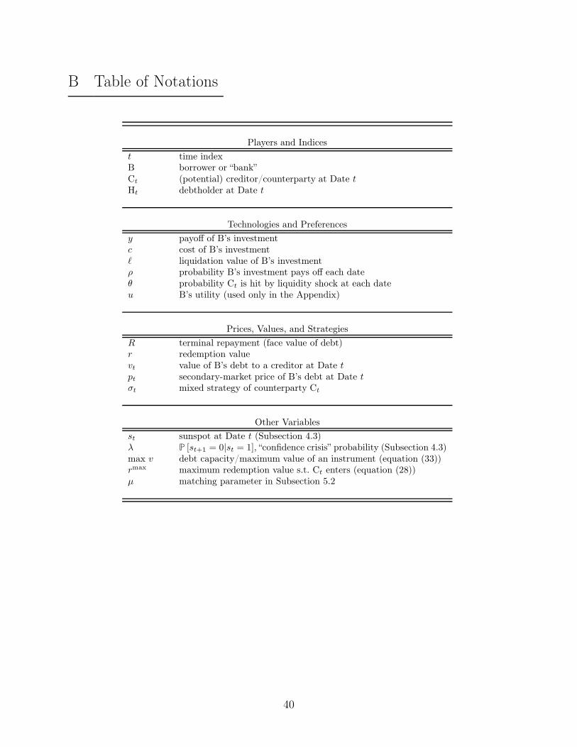
B Table of Notations

Players and Indices

t time indexB borrower or “bank”Ct (potential) creditor/counterparty at Date tHt debtholder at Date t

Technologies and Preferences

y payoff of B’s investmentc cost of B’s investmentℓ liquidation value of B’s investmentρ probability B’s investment pays off each dateθ probability Ct is hit by liquidity shock at each dateu B’s utility (used only in the Appendix)

Prices, Values, and Strategies

R terminal repayment (face value of debt)r redemption valuevt value of B’s debt to a creditor at Date tpt secondary-market price of B’s debt at Date tσt mixed strategy of counterparty Ct

Other Variables

st sunspot at Date t (Subsection 4.3)λ P [st+1 = 0|st = 1], “confidence crisis” probability (Subsection 4.3)max v debt capacity/maximum value of an instrument (equation (33))rmax maximum redemption value s.t. Ct enters (equation (28))µ matching parameter in Subsection 5.2

40

References

Acharya, Viral, Douglas Gale, and Tanju Yorulmazer, 2011, Rollover risk and market freezes,

The Journal of Finance 66, 1177–1209.

Allen, Franklin, and Douglas Gale, 1998, Optimal financial crises, The Journal of Finance

53, 1245–1284.

, 2004, Financial intermediaries and markets, Econometrica 72, 1023–1061.

Andolfatto, David, Ed Nosal, and Bruno Sultanum, 2017, Preventing bank runs, Theoretical

Economics forthcoming.

Antinolfi, Gaetano, and Suraj Prasad, 2008, Commitment, banks and markets, Journal of

Monetary Economics 55, 265 – 277.

Boyd, John H., and Edward Prescott, 1986, Financial intermediary-coalitions, Journal of

Economic Theory 38, 211–232.

Bruche, Max, and Anatoli Segura, 2016, Debt maturity and the liquidity of secondary debt

markets, Temi di discussione (Economic working papers) 1049 Bank of Italy, Economic

Research and International Relations Area.

Burdett, Kenneth, Alberto Trejos, and Randall Wright, 2001, Cigarette money, Journal of

Economic Theory 99, 117–142.

Calomiris, Charles W, and Charles M Kahn, 1991, The role of demandable debt in structuring

optimal banking arrangements, American Economic Review 81, 497–513.

Champ, Bruce, Bruce D. Smith, and Stephen D. Williamson, 1996, Currency elasticity and

banking panics: theory and evidence, Canadian Journal of Economics 29, 828–864.

Chemla, Gilles, and Christopher Hennessy, 2014, Skin in the game and moral hazard, The

Journal of Finance 69, 1597–1641.

Dang, Tri Vi, Gary Gorton, and Bengt Hölmstrom, 2015a, Ignorance, debt and financial

crises, Working paper.

, 2015b, The information sensitivity of a security, Working paper.

Dang, Tri Vi, Gary Gorton, Bengt Holmström, and Guillermo Ordoñez, 2017, Banks as

secret keepers, American Economic Review 107, 1005–29.

41

Diamond, Douglas W., 1984, Financial intermediation and delegated monitoring, The Review

of Economic Studies 51, pp. 393–414.

Diamond, Douglas W, 1997, Liquidity, banks, and markets, Journal of Political Economy

105, 928–56.

Diamond, Douglas W., and Philip H. Dybvig, 1983, Bank runs, deposit insurance, and

liquidity, Journal of Political Economy 91, 410–419.

Diamond, Douglas W., and Raghuram G. Rajan, 2001a, Banks and liquidity, The American

Economic Review 91, 422–425.

, 2001b, Liquidity risk, liquidty creation, and financial fragility: A theory of banking,

Journal of Political Economy 109, 287–327.

Donaldson, Jason Roderick, and Eva Micheler, 2016, Resaleable debt and systemic risk,

Working paper Washington University in St. Louis.

Donaldson, Jason Roderick, Giorgia Piacentino, and Anjan Thakor, 2017, Warehouse bank-

ing, Working paper Washington University in St Louis.

Duffie, Darrell, Nicolae Gârleanu, and Lasse Heje Pedersen, 2005, Over-the-counter markets,

Econometrica 73, 1815–1847.

Ennis, Huberto M., and Todd Keister, 2003, Economic growth, liquidity, and bank runs,

Journal of Economic Theory 109, 220–245 Festschrift for Karl Shell.

Farhi, Emmanuel, Mikhail Golosov, and Aleh Tsyvinski, 2009, A theory of liquidity and

regulation of financial intermediation, Review of Economic Studies 76, 973–992.

Friedman, M., and A.J. Schwartz, 2008, A Monetary History of the United States, 1867-1960

. National Bureau of Economic Research Publications (Princeton University Press).

Gorton, Gary, 1988, Banking panics and business cycles, Oxford Economic Papers 40, 751–

781.

, 1996, Reputation formation in early bank note markets, Journal of Political Econ-

omy 104, 346–97.

, and Andrew Metrick, 2010, Haircuts, Federal Reserve Bank of St Louis Review 96,

507–519.

42

, 2012, Securitized banking and the run on repo, Journal of Financial Economics

104, 425–451.

Gorton, Gary, and Guillermo Ordoñez, 2014, Collateral crises, American Economic Review

104, 343–78.

Gorton, Gary, and George Pennacchi, 1990, Financial intermediaries and liquidity creation,

Journal of Finance 45, 49–71.

Gorton, Gary B., 2012a, Misunderstanding Financial Crises: Why We Don’t See Them

Coming (Oxford University Press).

, 2012b, Some reflections on the recent financial crisis, NBER Working Papers 18397

National Bureau of Economic Research, Inc.

Green, Edward J., and Ping Lin, 2003, Implementing efficient allocations in a model of

financial intermediation, Journal of Economic Theory 109, 1–23.

Gu, Chao, Fabrizio Mattesini, Cyril Monnet, and Randall Wright, 2013, Banking: a new

monetarist approach, Review of Economic Studies 80, 636–662.

He, Zhiguo, and Konstantin Milbradt, 2014, Endogenous liquidity and defaultable bonds,

Econometrica 82, 1443–1508.

He, Zhiguo, and Wei Xiong, 2012, Dynamic debt runs, Review of Financial Studies 25,

1799–1843.

Iyer, Rajkamal, and Manju Puri, 2012, Understanding bank runs: The importance of

depositor-bank relationships and networks, American Economic Review 102, 1414–45.

Jacklin, Charles, 1987, Demand deposits, trading restrictions, and risk sharing, in Edward

Prescott, and Neil Wallace, ed.: Contractual Arrangements for Intertemporal Trade .

chap. II, pp. 26–47 (University of Minnesota Press: Minneapolis).

, 1989, Demand equity and deposit insurance, Working paper Stanford University.

Kiyotaki, Nobuhiro, and John Moore, 2001a, Evil is the root of all money, Clarendon Lec-

tures, Oxford.

, 2001b, Evil is the root of all money, Clarendon Lectures, Oxford.

, 2002, Evil is the root of all money, American Economic Review, Papers and Pro-

ceedings 92, 62–66.

43

, 2005, Financial deepening, Journal of the European Economic Association 3, 701–

713.

Kiyotaki, Nobuhiro, and Randall Wright, 1989, On money as a medium of exchange, Journal

of Political Economy 97, 927–954.

, 1993, A search-theoretic approach to monetary economics, American Economic

Review 83, 63–77.

Kozlowski, Julian, 2017, Long-term finance and investment with frictional asset markets,

Working paper New York University.

Krishnamurthy, Arvind, Stefan Nagel, and Dmitry Orlov, 2014, Sizing up repo, The Journal

of Finance 69, 2381–2417.

Kuong, John, 2015, Self-fulfilling fire sales: Fragility of collateralised short-term debt mar-

kets, Working paper.

Kučinskas, Simas, 2017, Liquidity creation and financial stability: The role of hidden trades,

Working paper University of Amsterdam.

Lee, Jeongmin, 2015, Collateral circulation and repo spreads, Working paper Washington

University in St Louis.

Leland, Hayne, and Klaus Bjerre Toft, 1996, Optimal capital structure, endogenous

bankruptcy, and the term structure of credit spreads, Journal of Finance 51, 987–1019.

Martin, Antoine, David Skeie, and Ernst-Ludwig von Thadden, 2014a, The fragility of short-

term secured funding markets, Journal of Economic Theory 149, 15 – 42 Financial Eco-

nomics.

, 2014b, Repo runs, Review of Financial Studies.

Peck, James, and Karl Shell, 2003, Equilibrium bank runs, Journal of Political Economy

111, 103–123.

Qi, Jianping, 1994, Bank liquidity and stability in an overlapping generations model, The

Review of Financial Studies 7, 389–417.

Ramakrishnan, Ram T S, and Anjan Thakor, 1984, Information reliability and a theory of

financial intermediation, Review of Economic Studies 51, 415–32.

44

Rocheteau, Guillaume, and Randall Wright, 2013, Liquidity and asset-market dynamics,

Journal of Monetary Economics 60, 275–294.

Sanches, Daniel, 2016, On the inherent instability of private money, Review of Economic

Dynamics 20, 198–214.

Sanches, Daniel R., 2015, Banking panics and protracted recessions, Working Papers 15-39

Federal Reserve Bank of Philadelphia.

Schmidt, Lawrence, Allan Timmermann, and Russ Wermers, 2016, Runs on money market

mutual funds, American Economic Review 106, 2625–57.

Singh, Manmohan, 2010, The velocity of pledged collateral, Working paper IMF.

, and James Aitken, 2010, The (sizable) role of rehypothecation in the shadow banking

system, Working paper IMF.

Sultanum, Bruno, 2016, Financial fragility in over-the-counter markets, Working paper Fed-

eral Reserve Bank of Richmod.

Thakor, Anjan, 2018, Post-crisis regulatory reform in banking: Address insolvency risk, not

illiquidity!, Working paper Washington University in St. Louis.

Trejos, Alberto, and Randall Wright, 1995, Search, bargaining, money, and prices, Journal

of Political Economy 103, 118–41.

Vanasco, Victoria, 2016, The Downside of asset screening for market liquidity, Journal of

Finance.

von Thadden, Ernst-Ludwig, 1999, Liquidity creation through banks and markets: Multiple

insurance and limited market access, European Economic Review 43, 991 – 1006.

45

money runs - giorgia piacentino - assistant professor of ... · money runs∗ jason roderick...

Documents