monitoring meadow vegetation response to restoration … · monitoring meadow vegetation response...
TRANSCRIPT
Monitoring Meadow Vegetation Response to Restoration in the Sierra Nevada
Technical Memorandum
Prepared for American Rivers 432 Broad Street
Nevada City, CA 95959
Prepared by Stillwater Sciences
2855 Telegraph Ave., Suite 400 Berkeley, CA 94705
November 2011

Technical Memorandum Monitoring Meadow Vegetation Response to Restoration
1 December 2011 Stillwater Sciences
i
Contact: Amy Merrill Stillwater Sciences 2855 Telegraph Avenue, Suite 400 Berkeley, CA 94705 (510) 848-8098 x 154 [email protected] Suggested citation: Stillwater Sciences. 2011. Monitoring meadow vegetation response to restoration in the Sierra Nevada. Prepared by Stillwater Sciences, Berkeley, California for American Rivers, Nevada City, California.

Technical Memorandum Monitoring Meadow Vegetation Response to Restoration
1 December 2011 Stillwater Sciences
ii
Table of Contents
1 PURPOSE AND NEED FOR A COMMON PROTOCOL FOR MONITORING
MEADOWS............................................................................................................................. 1
2 INTRODUCTION TO MEADOW VEGETATION MONITORING............................... 2
3 RESTORATION RESPONSE MONITORING STRATEGIES........................................ 3
3.1 Develop Restoration and Monitoring Plans Together ..................................................3 3.2 Gage Your Scale of Monitoring to the Expected Scale of Response ...........................4 3.3 Use Reference Sites to Inform Monitoring Plan...........................................................6 3.4 Establish Monitoring Before Changes to Management................................................6 3.5 Adaptive Management..................................................................................................6
4 LEVELS OF MONITORING: THE MONITORING PYRAMID.................................... 7
5 LEVEL 1: CHARACTERIZATION OF MEADOW VEGETATION ............................. 9
5.1 Introduction ..................................................................................................................9 5.2 Timing, Frequency and Expertise Required ...............................................................10 5.3 Data Collection Methods ............................................................................................10
5.3.1 Office preparation ................................................................................................10 5.3.2 Delineation of plant community type boundaries ................................................11 5.3.3 Plant community type data collection ..................................................................12 5.3.4 Field survey representative cross-sections ...........................................................13 5.3.5 Photo-point monitoring ........................................................................................13
5.4 Data Management and Analysis .................................................................................13 5.4.1 Recording field data .............................................................................................14 5.4.2 Plant Community Type Assignment and Description..........................................14 5.4.3 Elevation transect data .........................................................................................15 5.4.4 Plant Community Type Distribution and Extent..................................................16
5.5 Reporting ....................................................................................................................18 5.6 Personnel Requirements and Training........................................................................18
6 LEVEL 2: DECISION TREE FOR SELECTING METHODS TO MONITOR PLANT
COMMUNITY RESPONSE................................................................................................ 19
6.1 Decision Tree..............................................................................................................19 6.2 Study Design...............................................................................................................20 6.3 Basic Vegetation Measurement Methods: the Tool Box............................................22
6.3.1 Vegetation attributes to measure..........................................................................22 6.3.2 Methods for measuring vegetation attributes .......................................................24
6.4 Level 2 Monitoring Method Recommendations.........................................................26 6.4.1 Changes in meadow plant community type composition and distribution ..........26 6.4.2 Grazing impacts on vegetation composition ........................................................31 6.4.3 Biomass and nutrient content ...............................................................................32 6.4.4 Plant composition by Army Corps of Engineers wetland indicator status and/or
species diversity........................................................................................33

Technical Memorandum Monitoring Meadow Vegetation Response to Restoration
1 December 2011 Stillwater Sciences
iii
6.4.5 Floodplain vegetation sediment filtering and flood attenuation...........................34 6.4.6 Fire effects on vegetation .....................................................................................34 6.4.7 Edge tree dynamics ..............................................................................................35 6.4.8 Special-status species ...........................................................................................36 6.4.9 Invasive Species ...................................................................................................37 6.4.10 Riparian channel bank vegetation functions ........................................................38 6.4.11 Plant recruitment and survival .............................................................................39
7 REPORTING AND SHARING FINDINGS ...................................................................... 40
7.1 Monitoring Reports.....................................................................................................40 7.2 Sharing Findings in Monitoring Reports ....................................................................40 7.3 Data Storage and Data Sharing...................................................................................41
8 LITERATURE CITED ........................................................................................................ 42
TABLES
Table 1. Summary vegetation data for three plant community types . ..........................................15 Table 2. Five plant species in Meadow 8 in the Eldorado National Forest. ..................................15 Table 3. Relative elevations by plant community types………………………………………… 16 Table 4. Hypothetical plant community type extents. .................................................................. .16 Table 5. Matrix of monitoring methods and target vegetation attributes ………………………..24 Figures Figure 1. Process-directed monitoring goals and metrics are used to monitor restoration. ............7 Figure 2. Three-tiered approach to vegetation monitoring..............................................................9 Figure 3. Plant community types and other features for a meadow. .............................................17 Figure 4. Decision tree to guide Level 2 monitoring for restoration effects on vegetation...........20 Figure 5. Radial plot design. .........................................................................................................28 Figure 6. Sample graphic of change in dominant plant species cover…………………………...30 Appendices Appendix A. Level 1 Field Data Sheet Appendix B. Data Entry Forms Appendix C. Forage Nutrient Content Sampling and Analysis Appendix D. List of Common Meadow Plant Species and their seral and wetland status

Technical Memorandum Monitoring Meadow Vegetation Response to Restoration
1 December 2011 Stillwater Sciences
1
1 PURPOSE AND NEED FOR A COMMON PROTOCOL FOR MONITORING MEADOWS
The call for a consistent set of monitoring protocol(s) for both public and private meadows emerges from the need for rigorous, tractable and consistent monitoring at all rehabilitation1 sites to ensure that effects of management actions are well documented. Findings from designed and documented monitoring programs can be used to (1) guide adaptive management; (2) enable sharing of lessons learned among practitioners; (3) demonstrate benefits to local community members; and (4) demonstrate benefits of altered management to future funders. The purpose of this document is to present a vegetation survey protocol that can be applied across the Sierra Nevada to assess the short-term and long-term effects of meadow rehabilitation efforts. The overarching goal, as stated in the text of the National Fish and Wildlife Foundation (NFWF) proposal that funded this project, is to articulate methods for:
…. how to efficiently collect, analyze and report standardized data related to monitoring project impacts so that these data can be comparable across meadow projects. [With the ultimate goal that] results of meadow restoration efforts in the Sierra are quantified and reported in a consistent and comparable manner so that the benefits can be clearly articulated at a state and national policy level. [And so that] long-term comparable data sets revolving around key indicators are populated so that we can learn about long term restoration impacts, and adaptively manage these systems over time, particularly in light of climate change predictions.
Specific objectives and strategies stated in the NFWF proposal include coming to consensus on (emphasis added):
1. Data collection protocols for monitoring short-term (1–3 years) and long-term (4–10 years) project impacts on a small set of key indicators; and
2. Protocols for data analysis and reporting. The background discussion, decision tree, recommended methodology, field instructions, and field data sheets are the product of multiple discussions and email communications among the Vegetation Monitoring Review Committee, the members of which are listed below. The Vegetation Team has, to the degree possible, coordinated its methods and goals with the Hydrology and Wildlife Protocol Teams, such that these pieces can be brought together to produce an integrated understanding of a meadow system’s response to changes in management and/or actions intended to restore or rehabilitate meadow functions (hereafter referred to generically as “restoration”).
Name Affiliation(s)
Amy Merrill Stillwater Sciences
Athena Demetry National Park Service—Sequoia- and Kings Canyon
National Parks
Craig Oehrli USDA Forest Service LTBMU
Dave Weixelman USDA Forest Service
David Cooper Colorado State University
Julie Evans CNPS
1 Throughout this document, we use the term ‘rehabilitation’ to include preservation, enhancement, passive and active restoration.

Technical Memorandum Monitoring Meadow Vegetation Response to Restoration
1 December 2011 Stillwater Sciences
2
Name Affiliation(s)
Kathy Van Zuuk USDA Forest Service Tahoe National Forest
Leslie Mink Feather River CRM
Lisa Acree National Park Service—Yosemite National Park
Michele Hammond Bartolome Lab, UC Berkeley
Nick Jenson Veirs Lab, UC Davis
Sylvia Haultain National Park Service—Sequoia and Kings Canyon
National Parks
Todd Sloat Todd Sloat Consulting and FRRCD Coordinator
2 INTRODUCTION TO MEADOW VEGETATION MONITORING
There are many reasons one might want to monitor meadow vegetation response to restoration, as listed below (Pellant et al. 2005; Weixelman et al. 2003; Bombay et al. 2003; Craig and Williams 1998; Feather CRM 2010; Schlesinger 1997; Micheli and Kirchner 2002a, b).
• Plant species diversity
• Special status species population monitoring
• Forage production rates
• Carbon sequestration rates
• Vegetation response and effect on the fire regime
• Vegetation as indicator of ground water level
• Vegetation as indicator of wildlife habitat quality
• Vegetation density and rooting as indicator of erosion and sediment retention capacity Tractable monitoring information is critical for a particular restoration site for several reasons. Few if any restoration or enhancement projects require no management adjustments once the initial actions are complete. Monitoring can provide the critical information on which adaptive management decisions can be made; without such information, management becomes a combination of educated guesses and “seat of the pants” actions, which can produce unexpected results. One of the main purposes of monitoring is to provide an early warning for negative or unexpected changes in the meadow and to help identify ecological thresholds, beyond which changes in meadow processes can be more difficult to redirect. Examples of such “threshold” changes include channel incision, which once beyond a certain point (specific for each meadow) may continue, increasing channel depth and width unless major actions are taken (Chambers and Linnerooth 2001, Menke et al. 1996, Ratliff 1985). Another example is invasive plant species: beyond a threshold level of invasion (cover) species such as giant reed, Arundo donax, create physical habitat conditions that preclude growth and regeneration of other species while favoring expansion of Arundo (Coffman 2007). Identifying and incorporating these thresholds in a monitoring program make is possible for the manager to track when such thresholds are being approached, and thus to take early, preventative actions. Pre- and post-implementation monitoring information also provides evidence on how the restoration actions are affecting the site, including whether or not restoration goals and objectives are being achieved. The restoration and response story constructed of well collected monitoring

Technical Memorandum Monitoring Meadow Vegetation Response to Restoration
1 December 2011 Stillwater Sciences
3
data is far stronger and more convincing than one that is based upon photographs and personal observations. These kinds of evidence-based analyses are important for gaining support from funders, as well as local communities and other stakeholders. Findings from well planned and executed monitoring across many meadows also can be extremely valuable for understanding how and why meadows might vary in their responses to different management actions. Monitoring data collected using the same protocols can be used to compare meadow responses to management actions across sites with much higher resolution than when different protocols are applied because data will not have to be simplified into broader, common categories for analysis. This higher resolution of comparing and analyzing process responses across sites is important within a planning area or watershed, where understanding the condition and restoration effects of multiple meadows informs managers about habitat availability for mobile species (such as the great gray owl or willow fly catcher), basin-level effects on meadow ground water storage, and where restoration programs can be linked to other metrics, such as the cumulative downstream flow and sediment delivery effects of multiple meadow restoration projects within a single reach or tributary (ICF Jones & Stokes 2008). Systematic monitoring across multiple sites also supports the development of a more accurate understanding of how meadow responses can vary given differences in geology, alluvium, management history, hydrology, etc. This better scientific understanding can feed directly back into improved meadow management and predictions of what restoration actions might or might not be able to deliver. Funding mechanisms that recognize the importance of well-planned and executed pre- and post-project monitoring are needed to make such monitoring feasible for many practitioners.
3 RESTORATION RESPONSE MONITORING STRATEGIES
3.1 Develop Restoration and Monitoring Plans Together
In some cases, such as the San Joaquin-Sacramento Delta Levee Maintenance Subventions Program, long-term success (specifically defined) for wetland and riparian habitat restoration projects designed to mitigate for habitat destroyed during levee maintenance and repair must be documented in reports approved by California Department of Fish and Game (CDFG) and California Department of Water Resources (CDWR) within 3 years of receiving state funding; in these cases restoration project plans are developed in hand-in-hand with a monitoring plan (CDWR 2011). Funding for both is tied together. Pre-project monitoring provides essential information for developing restoration plans. In developing restoration and monitoring plans, it is helpful to keep three points foremost in mind: (1) start monitoring with pre-implementation data collection, (2) let project goals guide monitoring plans; and (3) tie monitoring design and metrics to restoration actions. These three points are elaborated upon below. Understand the kind of meadow with which you are working: Functional meadows in the Sierra Nevada and Southern Cascades of California are defined as landscape features with the following characteristics: (1) A meadow is an ecosystem type composed of one or more plant communities dominated by herbaceous species; (2) It supports plants that use surface water and/or shallow ground water (generally at depths of less than one meter) at some point during the growing season; (3) Woody vegetation, like trees or shrubs, may occur and be dense but are not dominant (Weixelman et al. 2011). Areas that have met these criteria in the past, but are currently in another ecological state due to alterations in hydrology and/or vegetation, but where changes in the current state could result in a land form that does meet the criteria listed above, are referred to as potential meadows.

Technical Memorandum Monitoring Meadow Vegetation Response to Restoration
1 December 2011 Stillwater Sciences
4
Different kinds of meadows (including fens with peat soils, lacustrine fringe [lake edge] meadows with sandy soils, and low gradient riparian meadows) are governed by different kinds of processes and process controls (e.g. types of ground or surface water input) and are subject to different kinds of impacts. Changing the management of mountain meadows in order to rehabilitate or restore meadow these various functions requires interpretation of site-specific information within the context of the meadow type and its potential. An excellent source for placing a meadow in a process-based classification is Weixelman et al. 2011. Do pre-implementation monitoring: Restoration plans need to be based on information about the site that has been gathered for as many years as possible prior to implementation. For meadows, it is especially important to understand the sources of existing stress on the system, as well as important structural features (texture of the underlying alluvium, ground water hydrology, and channel slope, geometry, etc.). When restoration directly or indirectly affects meadow hydrology, as is most frequently the case, collecting ground water and vegetation data during high, normal, and low water years is needed in order to provide a basis for comparison for the post-implementation observations. When pre-project NEPA/CEQA documentation data are required, use the same design and protocols planned for post-monitoring data collection; thus accomplishing two tasks in a single effort. Tie monitoring to goals: Meadow restoration goals are defined early in the project planning process and should be the starting point for development of any monitoring and adaptive management plan. These goals should be tied to improving or rehabilitating the natural meadow processes that create and maintain the desired conditions and/or structures. Tailor monitoring to restoration actions: There are a wide range of actions or alterations in management that fall under the rubric of meadow restoration. The expectation that certain management actions will affect specific outcomes in the meadow (structures and/or processes) represent hypotheses that need to be clearly articulated and monitored as directly as possible, before and after implementation, in order to ascertain whether or not the management actions had the desired effect. For example, monitoring the response to restoration of a floodplain that relies on passive revegetation will require tracking recruitment and survival of native and invasive plant species in the recreated floodplain. In contrast, monitoring a restored floodplain that has been actively revegetated will also require an assessment of the health and survival of the plantings as well as naturally recruited vegetation. Appropriate monitoring methods are dictated both by the restoration goals and the restoration actions. This is discussed in greater detail under Level 2 Monitoring in Section 6.
3.2 Gage Your Scale of Monitoring to the Expected Scale of Response
The need to detect important changes, as defined according to the project goals and objectives, requires matching pre- and post-implementation monitoring to the spatial and temporal scales at which these changes are expected to occur. Vegetation type conversion and large changes in forage production in response to broad scale changes in ground water levels would likely be best detected and monitored through stratified sampling within mapped polygons of vegetation type or using belt-transects with widely spaced vegetation plots. In contrast, plant biodiversity response to controlled burns could occur at the finer scales of pre-project fuel distribution, pre-existing soil moisture, and subtle variations in soil topography. Detection of such responses would require a finer-scale, spatially-focused sampling design.

Technical Memorandum Monitoring Meadow Vegetation Response to Restoration
1 December 2011 Stillwater Sciences
5
Similarly, the precision and associated sampling density needed for monitoring can be determined based on the expected degree of change or response of the meadow to restoration activities. For example, if restoration plans call for raising the ground water table from 10 to 2 ft below the surface throughout the growing season of a 100-ac meadow, the vegetation response expected would be extensive and profound, requiring a relatively low sampling density of dominant species cover to detect the change. In contrast, if restoration actions involve changing the grazing intensity or season, more subtle shifts in species composition might be expected and require more intensive monitoring such as permanent plot monitoring of all species occurrence in quadrats, or rooted density, to detect and track vegetation response. In order to assess the effects of restoration, baseline pre-implementation data must be collected across multiple water year types to document the natural inter-annual variation in species composition and productivity during wet vs. dry years. Monitoring programs should also be designed to accommodate the seasonal timing of plant response, and importance of vegetation response to specific events, such as flooding, fire, or grazing. In high elevation meadows, the growing season is so short and condensed, that it is generally possible to capture the majority of plant species in or near to flowering or fruiting between mid-July and mid-August; seasonal differences in early, mid and late bloomers increases as you descend towards sea level, and become much more important at and below 4,000 ft. Changes in response to grazing and other pressures or disturbances (e.g., flood, fire, forest clearing adjacent to or in the contributing area of the meadow) can be very important. For most cases, monitoring the site directly following a disturbance is an excellent way of observing how the restoration actions affected the meadow’s response to disturbance (and therefore effects on vulnerability and resilience). However interpretation of response to disturbance should be made with some understanding of the long-term trajectory and controls on the system. For example, over grazing and roads have exacerbated incision in many meadows in the Great Basin, but efforts to ‘restore’ channel form in these meadows should be performed and monitored with an understanding that the channels are also responding to a Holocene influx of sediment (Miller et al. 2011). Acknowledging and accommodating for event-driven monitoring in the budget and general project planning helps make these important data collection events happen. The duration of monitoring can also be tailored to expected response duration and to the timing of large events that can “test” the efficacy of restoration actions. You will be able to measure different changes over each time scale, for example, installed plant survival can be measured over a 1 to 3 year time scale, changes in conifer establishment rates will require longer time scales, such as 5 to 10 years, while changes in soil organic content might require even longer time scales. At a minimum, post-implementation vegetation monitoring should be performed for 3 continuous years, followed by less frequent monitoring, such as at 5-year intervals, as well as event-based monitoring. Monitoring directly following management changes can be targeted on the success of those management actions and coupled with frequent qualitative observations so that small negative changes are detected, and corrected, quickly; for example actively planted areas should be checked frequently for desiccation and herbivory. On-going effects of climate change, expected to include increasing temperatures and decreasing snow pack, are likely to continue, but with year to year variation, over the long-term and some climate change effects will be punctuated or, event-based, such as increased frequency of wild fire and rain on snow events. (Cayan et al. 2001, Mote 2006). Long-term monitoring at infrequent intervals, such as every five years, should be sufficient to capture meadow system responses to continuous effects of climate change; but event-based monitoring during or at an appropriate

Technical Memorandum Monitoring Meadow Vegetation Response to Restoration
1 December 2011 Stillwater Sciences
6
period following punctuated events will be required to measure responses to ‘pulse’ effects of climate change, such as catastrophic fires, rain on snow, or large floods.
3.3 Use Reference Sites to Inform Monitoring Plan
Identification, characterization and monitoring of one or several reference site(s), which represent(s) what is believed to be the target condition of the restoration site meadow is critical for establishing realistic restoration objectives and monitoring goals. Information from the reference site(s) can be used to understand composition, structure, and spatial and temporal variation of a ‘properly functioning’ meadow of the same type as the restored meadow. This information can be used to estimate acceptable levels of temporal and spatial variation in plant community composition and structure, and to help interpret vegetation responses to change. Specific characteristics and processes to measure in the reference site(s) need to be developed according to project needs. At a minimum, plant community composition in relation to plant water availability and soil texture should be assessed. Identification of appropriate reference site(s) must be done carefully and with a thorough understanding of both the project site and reference site(s) hydrology, geomorphology, and vegetation dynamics. As an initial framework, the hydrogeomorphic meadow classification developed by Weixelman et al. 2011 should be used.
3.4 Establish Monitoring Before Changes to Management
It is important to think through the monitoring design several years prior to implementation so that pre-implementation field measurements can be made during one or multiple season prior to implementation. These data will be extremely valuable for demonstrating meadow response to changes in management – the more years of pre-implementation data collected, the stronger the case for assigning meadow response to the management change rather than other time-related variables (e.g. climate). If possible a control site, which is as similar as possible to the target meadow but receiving no changes in management, can be monitored. Comparisons between the restoration site and the control site can help isolate responses to management from responses to interannual climatic variation. Use of a control site is suggested but not required for Level 1 monitoring. Such a design framework, in which a control and treatment (e.g., restored) area are monitored before and after treatment, is particularly powerful because it controls for effects due to both climatic variability and treatment (Stewart-Oaten, Murdoch, and Parker 1986, Stewart-Oaten and Bence 2001, Underwood 1994; Smith 2002).
3.5 Adaptive Management
The important relationship between restoration goals and objectives, monitoring, and adaptive management is depicted in Figure 1. Project goals for increased or decreased process rates or structural characteristics need to be translated into metrics with specific thresholds for action. For example, if a project goal is increased extent of Tahoe yellow cress (Rorippa subumbellata), then metrics, such as percent cover of that species overall and number of separate populations in the meadow, would be established, with specific action-thresholds, such as less than 3 separate populations within the meadow or less than 5% cover overall, that would trigger an adaptive management response. Within this framework, hypotheses about causal relationships among indicators and processes (e.g., seed production, germination, survival) can be articulated and
Technical Memorandum Monitoring Meadow Vegetation Response to Restoration
1 December 2011 Stillwater Sciences
7
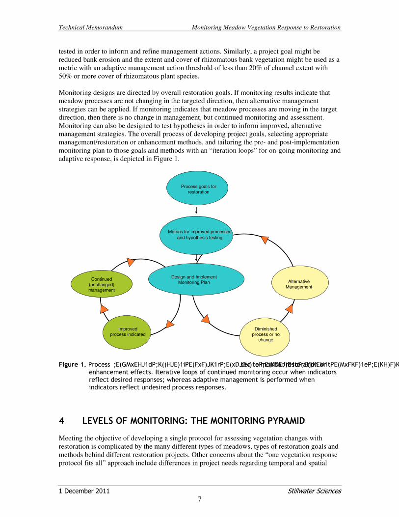
tested in order to inform and refine management actions. Similarly, a project goal might be reduced bank erosion and the extent and cover of rhizomatous bank vegetation might be used as a metric with an adaptive management action threshold of less than 20% of channel extent with 50% or more cover of rhizomatous plant species. Monitoring designs are directed by overall restoration goals. If monitoring results indicate that meadow processes are not changing in the targeted direction, then alternative management strategies can be applied. If monitoring indicates that meadow processes are moving in the target direction, then there is no change in management, but continued monitoring and assessment. Monitoring can also be designed to test hypotheses in order to inform improved, alternative management strategies. The overall process of developing project goals, selecting appropriate management/restoration or enhancement methods, and tailoring the pre- and post-implementation monitoring plan to those goals and methods with an “iteration loops” for on-going monitoring and adaptive response, is depicted in Figure 1.
Process goals for
restoration
Metrics for improved processes
and hypothesis testing
Improved process indicated
Diminished process or no
change
Alternative
Management
Design and Implement Monitoring Plan
Continued (unchanged)
management
Figure 1. Process directed monitoring goals and metrics are used to monitor restoration or enhancement effects. Iterative loops of continued monitoring occur when indicators reflect desired responses; whereas adaptive management is performed when indicators reflect undesired process responses.
4 LEVELS OF MONITORING: THE MONITORING PYRAMID
Meeting the objective of developing a single protocol for assessing vegetation changes with restoration is complicated by the many different types of meadows, types of restoration goals and methods behind different restoration projects. Other concerns about the “one vegetation response protocol fits all” approach include differences in project needs regarding temporal and spatial

Technical Memorandum Monitoring Meadow Vegetation Response to Restoration
1 December 2011 Stillwater Sciences
8
scales, levels of precision, and budget. Instead, the Review Team proposes a pyramid approach to monitoring meadow vegetation response to restoration. The pyramid (Figure 2) has three levels that, when applied, can yield increasing degrees of process-related information as well as require increasing levels of effort, technical expertise, and budget. The overall intent of the pyramid approach is to provide, at the first level, a consistent and informative but “low cost” common denominator monitoring method that could be applied across a wide array of meadow restoration efforts to coarsely characterize vegetation response to changes in management. This pyramid approach allows for increasingly focused levels of monitoring, from basic characterization (Level 1), to understanding system responses (Level 2), to testing specific hypotheses about meadow processes (Level 3). At Level 1, we propose a single universal method for describing general vegetation conditions that could be easily and inexpensively applied across all restoration sites expected to have large effects on meadow vegetation (e.g., purely in-stream restoration and/or measures not expected to affect ground water or floodplain conditions would not apply here). The Level 1 characterization would be useful for coarsely characterizing whole meadow vegetation under pre- and post-implementation, and, combined with other variables such as elevation, latitude, parent material and hydro-geomorphic context, will be useful for classifying unrehabilitated and restored meadows into like groups. We have made the Level 1 characterization as accessible and low-cost as possible while still providing important information that can support basin and region-wide meadow assessments. Level 2 monitoring targets meadow response to restoration actions and is, therefore, a fundamentally important part of adaptive management. Findings from these monitoring efforts, combined across different meadows where similar restoration goals and methods were applied, can provide critical information for improving restoration techniques. Level 3 methods, in which specific hypotheses about meadow processes (e.g., evapotranspiration rates, ground water-plant community interactions, plant community responses and controls, etc.) are articulated and then tested, can inform restoration methods, models and projections of meadow response to management actions, and changes in ecosystem services with differences in restoration actions. Each field protocol described in this document is also inextricably linked to methods for data analysis, reporting, and adaptive management. As discussed above, appropriate analysis, interpretation, and presentation of findings are critical and often under-appreciated steps of monitoring since without access to well-documented monitoring efforts, experiences cannot be shared and cannot evolve into lessons learned and improved management decisions. Thus, this final step, making monitoring reports and data available to others is crucial. In the following pages, we describe Level 1 monitoring methods for characterizing pre and post restoration meadow vegetation (Section 5); introduce and provide guidance on navigating the Level 2 decision tree for selecting appropriate response monitoring methods (Section 6); and describe reporting requirements and propose an approach to more open report and data sharing (Section 7). Level 3 monitoring methods are not prescribed since they are by nature specific to a project and the types of processes and questions being tested. Finally we provide Level 1 field data sheets in Appendix A.

Technical Memorandum Monitoring Meadow Vegetation Response to Restoration
1 December 2011 Stillwater Sciences
9
Level 3Hypothesis
Testing
Develop hypotheses and
specific methods to test
Level 2Response to Management Changes
Apply existing methods using scientific
approach and repeated measurements
Level 1Foundation: Core Characterization
Map distribution of vegetation types with dominant species; photo-stations; transects
Plant ID skills requiredInformation gained
Coarse shifts in
vegetation type and
distribution: Framework
Plant community responses
to different management
actions
Physical and plant
community interactions and process controls
Accurately identify
dominant species
(from local list)
Accurately identify
sedge and other
graminiod species
Accurately identify
sedge and other graminiod species
Figure 2. Three tiered approach to vegetation monitoring for meadows in the Sierra Nevada (conceptual design of pyramid scaled approach to monitoring is adapted from Land EKG, spring 2011 newsletter).
Although the Level 1 core characterization and Level 2 decision tree have been structured to accommodate a range of meadow sizes, complexity, budget capacity and botanical expertise, the group recognizes that the approach and methods for vegetation monitoring described in Sections 5 and 6 might require some changes and/or adaptations. We are hopeful, however, that such adaptations will be made conservatively and with broad communication among users in the Sierra Nevada, bearing in mind the importance of having consistently collected data sets for cross-comparison (in space and time) and to support broader understanding of meadow processes and response to restoration actions.
5 LEVEL 1: CHARACTERIZATION OF MEADOW VEGETATION
5.1 Introduction
The Level 1 characterization of meadow vegetation is basically a mapping exercise in which the distribution and boundaries of the different plant communities that make up the meadow mosaic are mapped, described, and linked to elevation transects. When applied over time, including one to several years before treatment as well as for multiple years following treatment, this level of monitoring can provide a powerful record of change. This Level 1 monitoring for meadow vegetation response to restoration should be performed in concert with the Level 1 monitoring for hydro-geomorphic response to restoration in which groundwater levels are recorded (American Rivers et al. 2011). Some of the questions that will be answered with this level of monitoring include:
• What are the dominant vegetation alliances in this meadow?
• What is their areal extent?
• What are relative elevations above channel baselevel associated with these alliances?

Technical Memorandum Monitoring Meadow Vegetation Response to Restoration
1 December 2011 Stillwater Sciences
10
• How has the extent and distribution of these vegetation alliances changed between pre- and post-project implementation, and as the project matures?
• At what rate have these changes occurred? In addition to answering the above questions, the information gathered through the Level 1 characterization will help land managers develop more specific management questions and hypotheses, such as: were observed changes in vegetation a response to management changes, or to particular weather patterns?; or to observed distribution of special features, such as springs, sediment deposits, etc.? Thus, the Level 1 characterization plant community type maps can be used as a framework for stratifying the meadow and pursuing more specific management response and process-oriented questions through Levels 2 and 3 monitoring. It is important for all restoration effects monitoring to clearly define the potentially affected area. In general, these should include all of the areas where any kind of treatment or change in management is planned and areas where the effects of such change will affect the physical template (water and or sediment availability and transport).
5.2 Timing, Frequency and Expertise Required
At a minimum, Level 1 Characterization monitoring is performed one year prior to initiation of changed management practices and/or restoration actions. Subsequent monitoring should occur at least during Years 1, 2, and 3 post-implementation and then at 5 yr intervals thereafter. Monitoring should be timed to plant phenology (e.g., flowering periods of the dominant plants species), so that changes in plant species composition can be attributed to management rather than seasonal differences among survey dates. Similarly, if the meadow is grazed, surveys should be performed either consistently prior to grazing, or consistently over one month following grazing so that plant flowering parts are available for plant identification and so that variability in inter-annual grazing effects do not confound findings on plant community extent and characterization. If possible a control site, which is as similar as possible to the target meadow but receiving no changes in management, can be monitored also. Comparisons between these sites can help isolate responses to management from responses to interannual climatic variation. Use of a control site is suggested but not required for Level 1 monitoring (refer to Section 3.3 above).
5.3 Data Collection Methods
There are five primary steps to collect data for characterizing meadow vegetation: (1) office preparation, (2) field delineation of plant community type boundaries, (3) plant community type data collection, (4) field survey representative cross-sections; (5) photo-point monitoring. These steps are described in greater detail below.
5.3.1 Office preparation
Prior to going out in the field, the team should acquire either most recent aerial imagery of the meadow to use as a field base photograph. NAIP or similar images (of equal or finer resolution) will be used to as a basis for delineating distribution of plant community types in the meadow. National Agriculture Imagery Program (NAIP) images have 1-m2 resolution and are produced under the auspices of the USDA’s Farm Service Agency (FSA), to provide aerial imagery of productive lands of the continental U.S. during the agricultural growing seasons. NAIP imagery is free and publically available in GIS-compatible format; other NAIP image formats that do not require GIS software can be purchased at low cost from private vendors. For more information on

Technical Memorandum Monitoring Meadow Vegetation Response to Restoration
1 December 2011 Stillwater Sciences
11
NAIP imagery coverage, format, frequency, cost, and websites from which to download NAIP imagery, see http://www.fsa.usda.gov/FSA/apfoapp?area=home&subject=prog&topic=nai. Prior to going out in the field, the team should print out a field base photo on 11x17 paper with a clear scale bar and north arrow. For large meadows (>100 ac) use several sheets of paper (< 50 ac per sheet) so that the hard copies are of sufficient resolutions for precise mapping. We recommend a map scale of at least 1:1,500 or finer for the field base photo. The field personnel should also familiarize themselves with local plant species common to meadows and grasslands and be familiar by sight with any potential threatened, endangered, or special status TES) species that might be encountered in the field. TES species found in the area can be listed by performing database search of the CNPS Inventory of Rare and Endangered Plants (http://www.rareplants.cnps.org/). The CNDDB and USFWS databases could also be queried following standard procedures2 and, if the meadow is on or near Forest Service lands, the local Forest Service botanist and wildlife biologist can be contacted for lists of potential species of concern. The field equipment, listed below, should be organized and made ready.
5.3.1.1 Field Equipment for Level 1 Monitoring
• Camera
• Clip board
• Compass
• Data Sheets
• Field Base-Photo
• Hand-held GPS
• Survey equipment
• Local plant species list
• Logging tape
• Pencils
• Permanent fine-tipped markers
• Plastic bags (for unknown plant samples)
5.3.2 Delineation of plant community type boundaries
Once in the field, the monitoring team should first walk through the meadow to understand the range of vegetation types (e.g. vegetation alliance and/or association per Sawyer, Keeler-Wolf and Evens 2009; see Section 5.5) and their distribution within the meadow mosaic. Based on this preliminary assessment, the team then identifies “stands3 representative of tentative vegetation
2 For standard CNDDB and CNPS database 9-quad search queries, see CNPS 2001:The CNPS Inventory of Rare and Endangered Plants; also available at: http://cnps.site.aplus.net/cgi-bin/inv/inventory.cgi. 3 Stand: A stand is a basic physical unit of vegetation in a landscape. It has no set size. A stand is defined by two main unifying characteristics: (1) It has compositional integrity. Throughout the site, the combination of species is similar. The stand is differentiated from adjacent stands by a discernable boundary that may be abrupt or indistinct. (2) It has structural integrity. It has a similar history or environmental setting that affords relatively similar horizontal and vertical spacing of plant species. In the case of meadows, look for areas with similar topography and access to ground and surface water. Areas along the meadow edge are also subject to different physical conditions (shade, conifer litter, etc.) (from CNPS 2011).

Technical Memorandum Monitoring Meadow Vegetation Response to Restoration
1 December 2011 Stillwater Sciences
12
types,” which are homogeneous in plant composition and structure. Within the meadow mosaic, you might have multiple stands (continuous patches) that are representative of different vegetation types. Mark vegetation type boundaries using an ultra fine point sharpie or similar permanent marker on the field base photo. If you have GPS and GIS capabilities, record the polygon outlines using a handheld GPS unit, noting the spatial precision and accuracy of your GPS at the site. For each polygon, locate easily visible points of reference in the field and on the aerial image, such as a lone conifer in the meadow, a large boulder, a road or trail, etc., and record the bearing and distance to the polygon’s closest edge from these reference points to tie your field location to points on the field base photo. The minimum mapping unit for these stands is suggested at 200 m2 (0.05 ac or 2,178 ft2). On the base photo (and if possible, in GPS), record the location of major stream channels as well as other important features such as gullies4, roads, trails, salt blocks, exclosure fencing, springs, etc. Based on field observations of dominant plant species, code the polygons on the field base photo according to a preliminary classification (e.g., beaked sedge, Lemon’s willow, Kentucky blue grass and slender wheat grass, corn lily and other dry forbs, etc.).
5.3.3 Plant community type data collection
Ground truth the plant community type polygon boundaries as delineated on the field base photo using the CNPS rapid assessment protocol (CNPS Vegetation Committee 2004). Select several polygons of each preliminary plant community type. At each of these polygons—or stands—record the occurrence and total percent cover of each of five plant groups as well as the percent cover of the dominant and characteristic plant species5. These plant groups are: (1) sedge and rush species; (2) other graminoid species; (3) forb species; (4) shrub (multiple stems) species; and (5) tree (single stem) species. In addition, record total percent cover of all moss and other non-vascular species. It is also very important to record total percent vegetation cover, as well as percent cover of bare mineral soil, bare organic soil, rock (gravel to boulder), and litter or thatch (see field base sheets in Appendix A). Ancillary information to collect for each representative stand could be extremely useful for interpreting vegetation response to management actions. Although not required at Level 1 monitoring, some easy and yet useful observations to record include surface soil moisture; surface soil texture (is it organic?); depth of organic or peat soil (using shovel, trowel or auger); slope and aspect; elevation relative to channel bottom (if site is along an elevation transect); presence or absence of rills and gullies and surface soil disturbance from rodents; and finally notes on land use and other sources of disturbance (see Appendix A for sample ancillary data sheet). While in the field, collect unknown plants that are important by their percent cover and/or frequency of occurrence. Be sure to know TES plant species so you don’t accidentally collect them. Press samples of the unknown species carefully in the field or put in a baggie and cooler until that evening. Identify or press within 24 hrs.
4 Gullies can be distinguished from channels because gullies do not have associated floodplains or well-vegetated banks; instead gully sides are made up of unsecured bare soil. 5 Dominant species include those with the greatest percent cover that also exceeds 10% per plant group; Characteristic species include those that occur with greatest consistency among stands – these do not have to have a high percent cover.

Technical Memorandum Monitoring Meadow Vegetation Response to Restoration
1 December 2011 Stillwater Sciences
13
5.3.4 Field survey representative cross sections
Development of several cross-sections, spanning from meadow edge to meadow edge and located at well chosen positions throughout the meadow, can provide the manager with rough estimates of plant community elevations above the groundwater. Placing the mapped plant community types along some or all of these transects increases the interpretive power of the mapped community types a great deal. Selecting transect locations is an important first step and should be done carefully, based on knowledge of the hydrology, geomorphology, and vegetation communities and with close attention to the planned on-the-ground restoration activities and restoration objectives for vegetation. The number of transects needed is a function of the complexity and size of the meadow. The smallest and simplest meadow would require three transects (top mid and lower meadow) but almost all meadows are likely to require more in order to capture the range of topographic variability in each meadow. Once transect locations are chosen, install permanent markers at the meadow edges of each transect and record the GPS points. Survey elevation changes along each transect; plant community type boundary positions should be recorded along each transect, as well as elevations on either side of each boundary. All transect elevations should be tied to a single reference elevation. Survey these transects before and after restoration activities, following any major storm or other disturbance events that affect meadow topography, and every 5 years following restoration.
5.3.5 Photo point monitoring
Photographs from multiple permanent points will be taken during each monitoring event. These are excellent sources of information when taken consistently from the same point and direction over time. Establish at least three permanent photo-monitoring points that capture the sweep of land in each meadow area of 25–30 ac. Photo-point positions and bearing (direction in which photographer is facing while taking picture) can be recorded on field base photo, using a hand-held GPS, and using permanent in-field markers such as fence stakes or wooden posts. However, realize that permanent field markers can be lost or destroyed during project implementation. During each monitoring event, record the date, location, and bearing of each photograph. It is very useful to place a white board with the date, location code, and bearing in the photograph itself (close enough to be legible on the photograph). Include the sky line at the top of each photograph. Photographs can be presented in a time-series in monitoring reports to illustrate overall change in vegetation cover and type (See Herrick et al. 2005a for details on a photo-point monitoring procedure).
5.4 Data Management and Analysis
Once collected, field data must be carefully preserved, analyzed, and reported in order to be of any use. The field base photo should be scanned and stored in digital form in a project folder. Most of the analysis for the Level 1 Characterization involves assigning plant community types to the stands identified in the field, recording and assessing the areal extent of each vegetation alliance either using GIS or by tracing polygons delineated on the base field photos, developing graphics showing elevation transects, and reporting relative elevations of plant community types.

Technical Memorandum Monitoring Meadow Vegetation Response to Restoration
1 December 2011 Stillwater Sciences
14
5.4.1 Recording field data
Once back from the field, unknown plant species should be identified and corrected species names recorded along side the field recorded names on the field data sheets. All plant names for dominant species need to be recorded to the species level using the Jepson Manual naming conventions (Hickman 1993, or as updated on the Jepson online interchange: http://ucjeps.berkeley.edu/interchange.html; Rosatti 2003). The botanist should record their initials and date next to each plant name correction or update. Once these corrections have been made to the field data sheets, these should be scanned and stored in digital form. Species names and percent cover estimates per stand should then be entered into an excel file according to the format provided in Appendix B, Tables B-1 and B-2. If GIS capabilities are available, it is best to digitize the polygon outlines recorded in the field on the field base photo using the NAIP imagery as a backdrop and to attribute each polygon with a unique polygon code and with a plant community type code, as described in the next section. Name this GIS layer to include the field dates of data collection. This layer can be used to quantify the extent of each community type in the meadow, and by comparing such layers over time, to quantify changes in extent and distribution of plant community types.
5.4.2 Plant Community Type Assignment and Description
Use field information on the most consistent and/or dominant plant species per stand to make a determination of the alliance level names according to the Manual of California Vegetation (Sawyer et al. 2009). To assign plant community types to your field polygons, match the published plant community type descriptions based on geographic distribution, and dominant and co-occurring species. Use the second edition of the Manual of California Vegetation (MCV2; Sawyer et al. 2009) as a first reference for plant community types and assign vegetation community class names to at least the alliance level; in some cases it may be possible to assign to the association level6. Other more local classifications might be available through the Forest Service (e.g., Potter 2005, primarily presented at the association level), and can also be used. Be sure to fully cite the sources of each published plant community type used. Because the classification for meadow vegetation for the Sierras is incomplete, some observed plant communities will not fit those described in the MCV2 or other published meadow classifications. In these cases, names should be applied according to the CNPS naming convention in which characteristic species of the upper most important vegetation layer are used in the alliance name and the most characteristic species in two vegetation layers are used to assign the association name. For example a stand dominated by showy sedge (Carex spectabilis) sod belongs to a well-documented alliance referred to as the Carex spectabilis Herbaceous Alliance (Sawyer et al. 2009); and Salix jepsonii/Senecio triangularis is a plant association described in Potter (2005). Include the word “Proposed” in any alliance or association you name yourself; e.g., Carex simulata/ Oreostemma alpigenum
7 Proposed Association. Record the level of confidence you have in the assigned alliance or association name (high, medium, or low confidence).
6 Alliance (or series) level vegetation classes are identified by the plant species that is dominant in the layer with the greatest cover (tree, shrub, or herbaceous layers). Associations are classified at a finer scale than alliances and are classified based on groups of commonly co-occurring species which generally includes characteristic species in more than one vegetation layer Sawyer et al. 2009). 7 Formerly Aster alpigenus.

Technical Memorandum Monitoring Meadow Vegetation Response to Restoration
1 December 2011 Stillwater Sciences
15
Summarize the cover categories for each community type observed in the meadow by presenting the mean (and standard error if possible) of each for the stands measured. These can be presented in a single table (see Tables 1 and 2 below). Table 1. Summary vegetation data for three plant community types sampled within Meadow 8
during late summer 2010 in the Eldorado National Forest.
Sed
ge
an
d r
ush
Gra
ss
Fo
rb
Sh
rub
Tre
e
Ba
re g
rou
nd
Ro
oti
ng d
ensi
ty
sum
%F
AC
W
OB
L
Mea
do
w
Com
mu
nit
y c
od
e
Percent Cover Mea
do
w c
om
mu
nit
y
typ
e
8 A 5–15 1–5 25–50 1–5 1–5 1–5 High 89 Wet
8 B 25–50 0–1 50–75 0 0 1–5 High 90 Wet
8 C 25–50 0–1 5–15 1–5 0 0–1 High 80 Wet
Table 2. Five plant species with the greatest absolute percent cover in the plant community types observed in Meadow 8 during late summer 2010 in the Eldorado National Forest.
Meadow Community
code Species 1 Species 2 Species 3 Species 4 Species 5
8 A Aster
alpigenus
Mimulus
primuloides
Carex
nebrascensis
Polygonum
bistortoides
Vaccinium
uliginosum
ssp.
occidentale
8 B Carex
nebrascensis
Polygonum
bistortoides
Potentilla
gracilis
Senecio
triangularis Moss
8 C Aster
alpigenus
Polygonum
bistortoides
Saxifraga
aprica Carex illota
Senecio
triangularis
5.4.3 Elevation transect data
Once in the office, completed transect data sheets should be copied and electronically scanned and the originals safely stored. Data should then be entered (with a QA/QC check) and elevations calculated for each point relative to the channel base level along the associated transect (each of these values should also be linked to a single reference point elevation). Calculate relative elevations (average and standard deviation) for each community type polygon with at least three surveyed points along each transect. Report the relative elevation for each polygon by vegetation type (average, standard deviation, number of points per vegetation type within a polygon). These data can be further summarized to the vegetation type level by presenting averages and standard deviations per vegetation type. An example results table is presented below (Table 3).

Technical Memorandum Monitoring Meadow Vegetation Response to Restoration
1 December 2011 Stillwater Sciences
16
Table 3. Relative elevations recorded by plant community types in a hypothetical meadow average (standard deviation, number of samples); elevations given in feet above channel base
level within the transect, as recorded on June 11, 2011.
Meadow
Plant
community
type
Polygon 1a,
Transect 1
Polygon 1d,
Transect 1
Polygon 3c,
Transect 3
Polygon 6d,
Transect 6
Combined
Polygons
Golden Meadow
Veratrum
californicum-
Polygonum
bistortoides
3.2 (+1.4, 3) 4.1 (+2.2, 4) 2.5 (+1.1, 5) 3.1 (+0.8, 5) 3.2 (+ 1.4, 4)
Golden Meadow
Artemisia
tridentata/Poa
secunda 6.1 (+2.1, 4) 6.5 (+2.8, 5) 5.8 (+2.1, 4) na 6.1 (+ 2.3, 3)
Golden Meadow
Artemisia
tridentata/
Leymus
cinereus
8.5 (+3.4, 5) 9.1 (+3.4, 4) 8.8 (+2.8, 3) 10.1 (+4, 3) 9.1 (+ 3.4, 4)
5.4.4 Plant Community Type Distribution and Extent
Measurements of plant community distribution can be made by either querying the polygon layer created in Section 5.4, or by measuring the polygon areas the “old fashioned way” with an acetate sheet of squares of known size (e.g., 4 m2 based on the scale of the field base map) overlaid on the field base photo and counting the total number of squares in each vegetation type (Dunne and Leopold 1978). Once completed, the aerial extent of each vegetation type can be reported in a summary table. These values can be presented to show change with implementation and over post-implementation years, as illustrated in Table 4.
Table 4. Hypothetical plant community type extent as measured pre and post restoration for a 100 ac meadow; areas presented in acres.
Y 2 Pre Y 1 Pre Y 1 Post Y 2 Post Y 3 Post Y 8 Post Plant community type
Acres
Artemisia tridentata/Poa secunda 77 80 10 4 5 2
Artemisia tridentata/ Leymus
cinereus 20 17 5 2 3 1
Juncus nevadensis 2 1 15 12 12 12
Carex nebracensis 1 2 35 42 40 45
Veratrum californicum-Polygonum
bistortoides 0 0 15 12 14 12
Senecio triangularis-Athyrium
filix-femina 0 0 12 20 20 22
Open water 1 1 8 8 8 8
Total 100 100 100 100 100 100
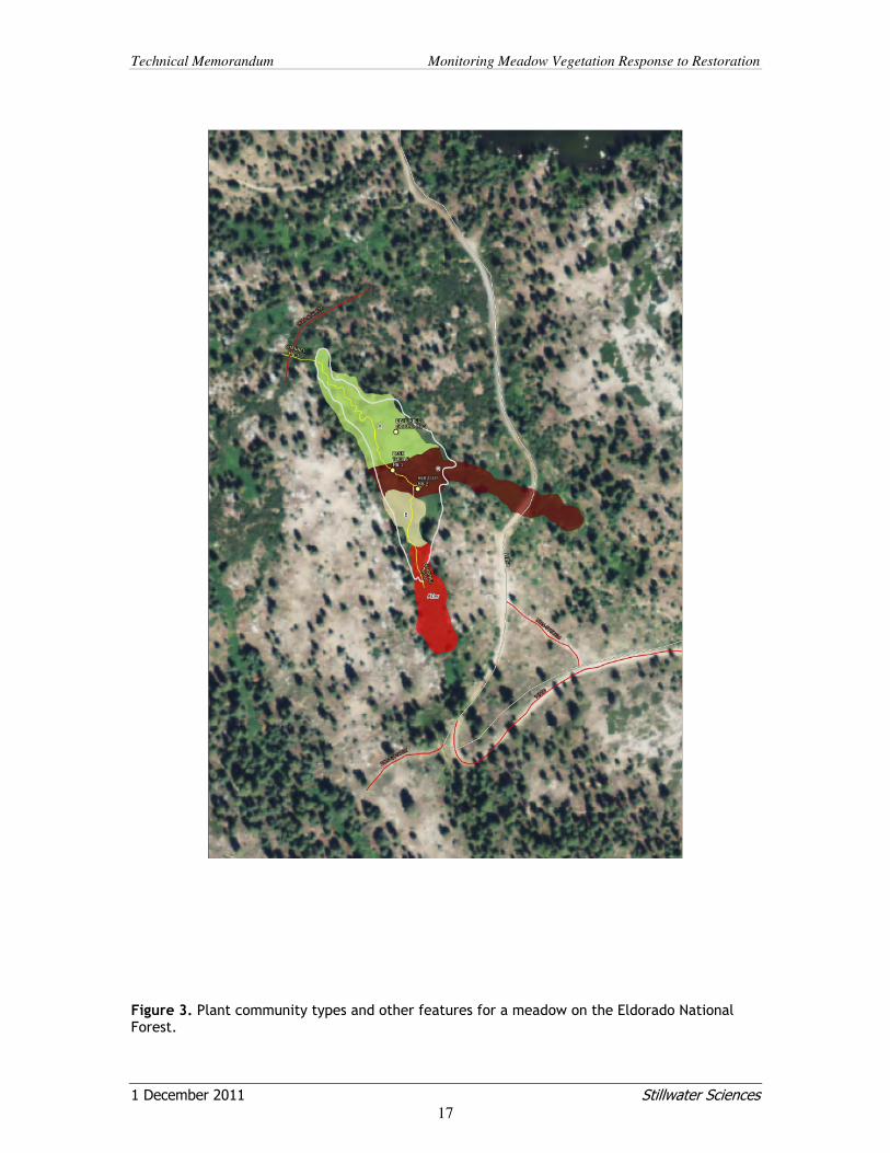
A figure, showing the plant community type polygons, as coded in the associated tables is also an excellent way to present the distribution and extent of vegetation types. For example, Figure 3 illustrates the distribution and extent of meadow plant community types in one meadow on the Eldorado National Forest. This figure also shows roads and trails, hydro-geomorphic features, as well vegetation community types summarized in Tables 1 and 2.
Technical Memorandum Monitoring Meadow Vegetation Response to Restoration
1 December 2011 Stillwater Sciences
17
Figure 3. Plant community types and other features for a meadow on the Eldorado National Forest.

Technical Memorandum Monitoring Meadow Vegetation Response to Restoration
1 December 2011 Stillwater Sciences
18
5.5 Reporting
Pulling monitoring information into a well-documented report, including field data, photographs, figures of the plant community type polygons and a summary assessment, is a critical step. We recommend that monitoring reports be updated annually for at least the first three years following a major change in management and at five year intervals thereafter. Each year of monitoring data should be added into the previous report, so that the full history of monitoring and response is in a single document. A possible format for such a report is:
1. Title, including date, authors and any associated institution, contact information
2. Introduction: Location, size, ownership, brief overview of restoration and/or management history.
3. Purpose, goals, and implementation dates for change in management.
4. Methods used for monitoring (this can briefly refer to this or other document while providing details on specific methods applied in the field).
5. Results section should provide a discussion of problems encountered in the field or analysis, as well as
a. Summary tables of plant community types for each year of monitoring;
b. Plant community type information, per year of monitoring;
i. Areal extent;
ii. Dominant species and vegetation; and
iii. Bare ground, litter, and rock cover.
c. Figure(s) showing aerial photograph or NAIP image with delineated plant community type boundaries and codes;
d. Ancillary data on ground water levels, elevation, soil texture, etc.; and
e. A map of the meadow showing location of permanent photo-points and photograph series from permanent photo-monitoring sites.
6. Discussion, including interpretation of plant community types in relation to management conditions, possible explanations for any observed changes in plant community types and/or distributions.
7. Literature cited.
8. Appendices (with scanned field data sheets, full plant species lists, other photographs, etc.).
Vegetation field data, photo-monitoring images, NAIP images with community type boundaries, and GIS layers should be archived in a safe and accessible location. Preferably, several hard copies of the report that include CD’s with the associated data could be submitted to a Meadow Database and Library for off-site safe storage (See Section 7).
5.6 Personnel Requirements and Training
For meadows that are roughly 40 ha or less (100 ac), this level of monitoring should require a total of two days of both office and field time including transect surveys. We recommend that the Level 1 field monitoring be performed by a team of at least two personnel to increase efficiency and to provide two perspectives at the junctures where judgment is required (e.g., delineating plant community type boundaries). Moreover, it is simply helpful to have two sets of hands to set up transects and to observe/record field data. At least one of the field people must have strong

Technical Memorandum Monitoring Meadow Vegetation Response to Restoration
1 December 2011 Stillwater Sciences
19
local botanical skills, including knowledge of local graminoid (sedge) species. Having GIS software and some entry level to moderate GIS capability would also make some of the spatial analysis easier, but is not necessary.
6 LEVEL 2: DECISION TREE FOR SELECTING METHODS TO MONITOR PLANT COMMUNITY RESPONSE
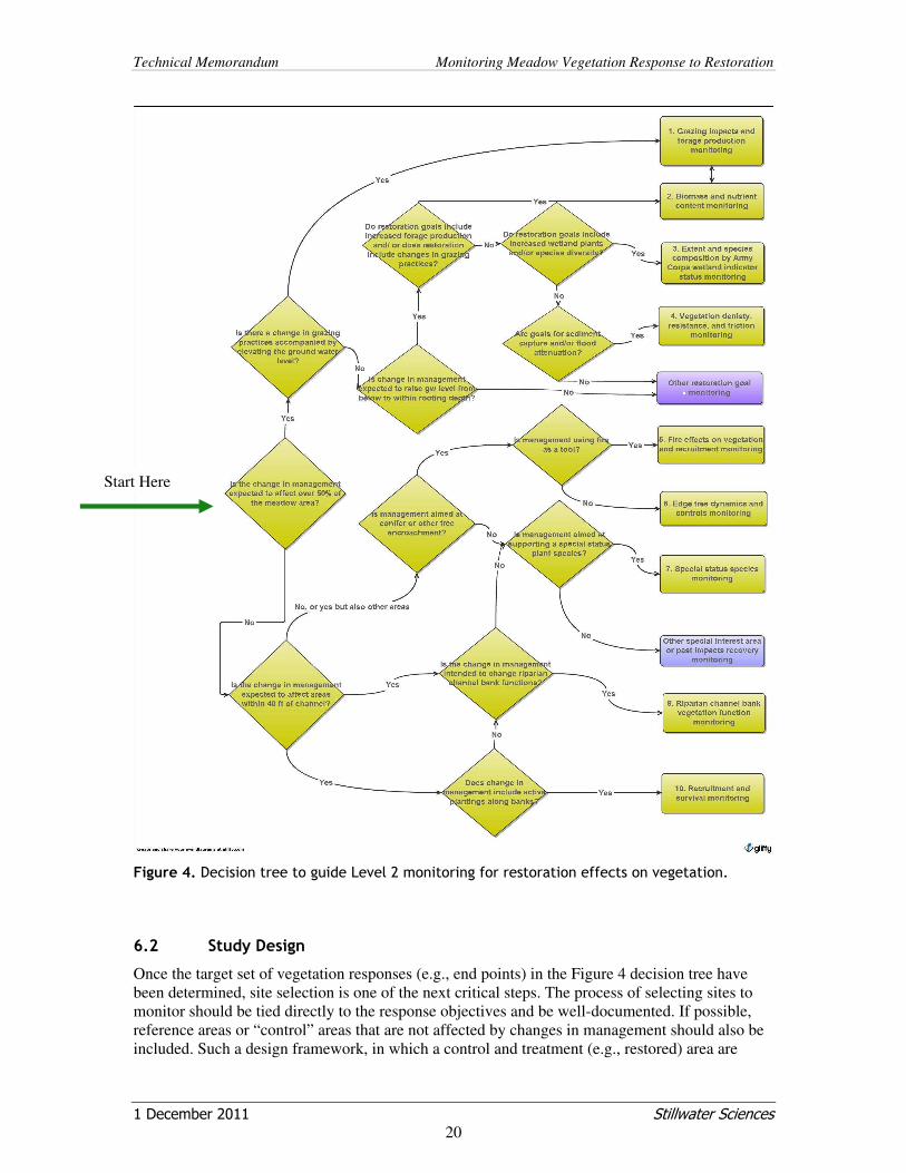
Level 2 monitoring targets meadow response to restoration actions and is, therefore, a fundamentally important part of adaptive management. Findings from these monitoring efforts, combined across different meadows where similar restoration goals and methods are applied, can also provide critical information for improving restoration techniques. The decision tree in Figure 4 is based on management goals and techniques, and is designed to guide the meadow manager to information resources useful for developing appropriate monitoring protocols. In many cases, the protocols might require tailoring to the specific needs and characteristics of the meadow.
6.1 Decision Tree
Following the decision tree diagram, we discuss common monitor design issues, such as size, shape, intensity and distribution of measurement areas, monitoring frequency and timing, and offer a tool box of commonly applied vegetation measurement methods. In the last part of Section 6, we review specific existing vegetation monitoring methods tiered to the decision tree, and discuss how they can be best applied to meadow vegetation response monitoring. For each method, the reader is referred to existing publications and protocols for detailed discussion and field data sheets.
Technical Memorandum Monitoring Meadow Vegetation Response to Restoration
1 December 2011 Stillwater Sciences
20
Figure 4. Decision tree to guide Level 2 monitoring for restoration effects on vegetation.
6.2 Study Design
Once the target set of vegetation responses (e.g., end points) in the Figure 4 decision tree have been determined, site selection is one of the next critical steps. The process of selecting sites to monitor should be tied directly to the response objectives and be well-documented. If possible, reference areas or “control” areas that are not affected by changes in management should also be included. Such a design framework, in which a control and treatment (e.g., restored) area are
Start Here

Technical Memorandum Monitoring Meadow Vegetation Response to Restoration
1 December 2011 Stillwater Sciences
21
monitored before and after treatment, is particularly powerful because it controls for effects due to both climatic variability and treatment. This design is referred to as the “Before-After-Control Impact” design (Stewart-Oaten et al 1986). Sampling sites should also be well distributed throughout the affected (and control) areas using a stratified random sampling design so that you can infer that your measurements represent the greater affected or control area. Stratifying the meadow by vegetation type within the mosaic could, in most cases, capture the major drivers of variation in response to management since vegetation type distribution is an integration of hydrology, soils, and management history. However, if there are other variables within the meadow that are expected to explain more of the variation in response to management change, then use these with a clear and explicit rationale for why you are selecting this other variable over vegetation type for stratification. Once the monitoring sites have been identified, selecting specific plot locations within these areas should, generally, be done randomly. Finally, choosing between permanent vs. temporary sampling locations can also have important implications for interpretation of the data you collect. Data collected from different, randomly selected plots on each sampling date are independent of one another but data collected from permanent plots are dependent on or linked, to the data collected on previous dates. Smaller changes in vegetation compared across sample dates in permanent plots will therefore be more likely to indicate a real response then will the same size changes in randomly located plots across sample dates. In short, permanent plots can give your monitoring system greater sensitivity to vegetation change. However, practical concerns also need to be considered; such as whether or not the pre-implementation site locations will be appropriate for monitoring under post-implementation conditions, the time required to install and remove permanent plot markers, and whether or not land owner permission for installing permanent markers will be granted. Some meadows, including fens, have peat soils that are easily compacted and therefore could be damaged by the repeated trampling associated with permanent plots. In these cases, temporary plots might be preferable. Alternatively, temporary boardwalks to the sampling sites can be erected to protect the soil and local hydrology from sampling damage. The distribution and number of plots will affect and precision with which the data collected represent overall conditions; the need for having a sample size large enough to detect changes must be balanced with associated costs and labor. Generally, larger sample sizes increase the likelihood that smaller changes or responses will be detected. Methods exist for determining the appropriate sample size, given a target degree of precision needed (e.g., 10% change) and variation within the target vegetation types. Estimates of spatial variability can be developed based on other monitoring reports or published studies of the target or similar vegetation types. A description of these methods can be found in Chapters 7 and 8 and Appendix 7 of Elzinga et al. 1998. The size of the measurement areas or plots also importantly affects how well the data collected reflect the population response to treatment. Recommendations on sample plot size are provided below with specific methods, as well as in the sources referenced in this document. Other aspects of the overall sampling design include the resolution of sampling itself. Do you sample all plant species or groups of species based on wetland indicator status, seral status, vegetation layer (shrub, tree, graminoid, etc.), specific morphology (e.g., rhizomatous or clonal species), or age cohort (tree seedling, sapling, pole, or “mature” sized), etc.? This decision has implications for the degree of training and experience required of the field personnel and of the amount of post-field plant identification time that might be required.

Technical Memorandum Monitoring Meadow Vegetation Response to Restoration
1 December 2011 Stillwater Sciences
22
For each of the target responses, we provide guidance on these study design decisions in Section 6.4 below. More in-depth discussions and advice on how to best tailor these decisions to your particular project can be found in existing publications and will not be repeated here (see Elzinga et al. 1998 [Chapter 7]; Coulloudon et al. 1999 [Chapter 3]; and Herrick et al. 2005a,b).
6.3 Basic Vegetation Measurement Methods: the Tool Box
Many of the measurement methods for monitoring vegetation response to restoration or change in management are based on a few basic methods used to characterize or quantify changes in vegetation in a given area. These are listed and briefly described below. Suggestions on how and when to apply these methods in order to address target vegetation responses to management (Figure 4) are provided in Section 6.4. For more detailed descriptions of each method, including specific field gear required, field methods, field data sheets, and data analysis and reporting methods go to Elzinga et al. 1998; Coulloudon et al. 1999; or Herrick et al. 2005a,b.
6.3.1 Vegetation attributes to measure
6.3.1.1 Plant identification
This fundamental attribute is critical because it determines the level of resolution of your vegetation data and the level of expertise, and expense, for the field sampling effort. The expertise required will vary based on project needs but must be carefully considered. Options range from the general categories such as plant groups [(1) sedge and rush species; (2) other graminoid species; (3) forb species; (4) shrub (multiple stems) species; (5) tree (single stem) species and (6) bryophyte cover] requiring the least expertise, to plant species, subspecies and variety including bryophytes, requiring the highest level of expertise. Variations in between include identification of dominant species (over 10% cover) excluding bryophytes, or identification of genera present, etc. Identification to the species and subspecies or variety is usually required in order to determine the wetland indicator status8 or seral status9 of the plant. These categories are helpful in that they (generally) can be used to infer information about site conditions. A list of common meadow species, their wetland indicator and seral status is provided in Appendix D (developed by Region 5 of the USDA Forest Service; D. Weixelman, US Forest Service, pers. comm. with A. Merrill, Stillwater Sciences, 27 October 2010). In many cases in which plant species are measured as indicators of site conditions, and/or vegetation biodiversity, identification to the species level will be needed. In these instances, use nomenclature according to Hickman 1993 for all vascular plant species names, or when available, the 2011 Jepson Manual, 2nd Edition (see also Jepson Interchange: http://ucjeps.berkeley.edu/interchange.html; Rosatti 2003). There has also been growing interest and expertise in non-vascular plants (mosses and other bryophytes) as indicators of site conditions, particularly in fens. To this extent, total bryophyte cover can be recorded in the field along with other plant information. Identification of bryophytes by species is an uncommon (but growing) form of expertise. If field personnel do not have this expertise, and it has been determined that bryophyte species differences are important monitoring
8 Wetland indicator status of each species is published by the Army Corps of Engineers for each region of the Country. Categories are OBL [obligate], FACW [facultative wet], FAC [facultative], FACU [facultative-upland], and UPL [upland]) using the 1988 national list of plant species that occur in wetlands for Region 0 (Reed 1988). 9 Region 5 of the USFS has developed a list of common meadow species and their associated seral status (early, mid, and late successional) when found in wet, mesic, and dry meadows.

Technical Memorandum Monitoring Meadow Vegetation Response to Restoration
1 December 2011 Stillwater Sciences
23
targets, then distinctly different types of bryophytes can be given unique field codes and samples collected in the field. These samples can then be sent for identification by bryophyte experts (also, see Doubt and Belland 2000).
6.3.1.2 Frequency
Frequency reflects the number of times a species is present in a given number of sampling units, and is usually expressed as a percentage of the total number of samples collected (Elzinga et al. 1998). While rooted frequency is the most sensitive parameter of vegetation response, it does not reflect important differences in biomass or plant cover. Seedlings can also heavily skew data and seedling density should be collected separately or in such a way that seeding data can be separated from the rest of the numbers. Sample sizes need to be identical across areas being compared and must be large enough to incorporate “clumping patterns” of different species. When paired with cover or production data, frequency measurements can be very sensitive to small changes in vegetation.
6.3.1.3 Cover
In general, cover is the amount of a given area covered by one or all plant species in a plot. However, cover can be presented in multiple forms. Foliar cover is the area of ground covered by vertical projection of the aerial parts of plants, whereas basal cover is the area of ground surface occupied by the basal portion of the plants. Foliar cover is more sensitive to climatic variations and current-year grazing. Ground cover is the most stable since it is less responsive to current-year grazing and variations in climate, however measurements of basal cover require more time and labor, especially in herbaceous plant communities, than foliar cover. Once again, precision requirements must be balanced with available time and budget.
6.3.1.4 Density
Density refers to the number of individual plants in a given area. Density is therefore an indicator of proximity among individuals and can be interpreted with resource availability. Differences in individual size (e.g., seedling vs. mature tree), reproductive methods and structure (multi or single –stemmed) can make interpretation of results more difficult.
6.3.1.5 Production or Standing crop
Production refers to the amount of plant biomass produced in a given time period. Most frequently, only annual above-ground production is measured and in herbaceous communities. In such cases peak standing crop, the greatest amount of plant biomass present above ground during a given year, is typically used to estimate above-ground production. Peak standing crop generally occurs towards the end of the growing season, but different plant species peak at different times. Total forage is the total amount of herbaceous and woody palatable plant biomass available to herbivores. Variation in standing crop is introduced by climatic variability, grazing, insect herbivory, trampling, and time of sampling.
6.3.1.6 Structure
Vegetation structure describes the vertical and horizontal distribution of vegetation. Vegetation layers are generally defined by height above ground and measured by percent cover in each layer. Vegetation structure is important for fire as well as wildlife habitat needs.

Technical Memorandum Monitoring Meadow Vegetation Response to Restoration
1 December 2011 Stillwater Sciences
24
6.3.1.7 Composition
Composition refers to the different plant species in a given area and the relative proportion of space (canopy or basal cover) and/or biomass that they comprise. Composition is measured using species-specific cover or frequency data collection methods.
6.3.1.8 Vigor
Growth rate, as measured either within a single growing season or for woody species, across growing seasons can be an excellent indictor of plant vigor and can be measured as vertical change and/or as an increase in canopy circumference, as measured by two orthogonal measurements of canopy width. Other metrics of overall plant vigor can also include number of leaves or whorls, percent of foliage that is healthy (with clearly defined categories for each vigor stratum), or number of inflorescences per plant (see Elzinga et al. 1998 [Chapter 8]).
6.3.1.9 Riparian canopy light interception
Riparian canopy interception is a less commonly used, but still an important metric for riparian restoration projects where channel water temperature is an important condition for aquatic species. Riparian canopy interception is measured based on the percent of channel surface area shaded by plants. Deciduous plants provide shade only during the growing season, where as evergreens provide year-round shade. The position of the vegetation in relation to the path of the sun importantly affects the amount of radiant energy the plants intercept above the water surface.
6.3.2 Methods for measuring vegetation attributes
Hundreds of specific field methods have been developed for particular riparian and rangeland monitoring applications. These can be grouped into a handful of methods categories that can be adapted to measure the vegetation attributes described above. Table 5 lists these types of methods and the vegetation attributes they can be used to measure. These can all be tailored to monitor the specific vegetation responses to management actions listed in Figure 4. A brief description of each method is provided below, along with a publication that offers more detailed descriptions, diagrams, and field sheets. A review of a similar set of methods for riparian areas in general is also publically available and should be reviewed along with this document (it is only 17 pages long; National Riparian Service Team. 2004).
Table 5. A matrix of monitoring methods (rows) and target vegetation attributes (columns).
Attributes (across)
Methods (below)
Fre
qu
ency
Co
ver
Den
sity
Pro
du
ctio
n
Po
pu
lati
on
siz
e
an
d e
xte
nt
Str
uct
ure
Com
po
siti
on
Vig
or
Rip
ari
an
lig
ht
inte
rcep
tion
Photo-points
Rooted frequency x x x x
Line intercept x x x
Point intercept x x x
Belt transect x x
Standardized unit effort x
Harvest x
Greenline x x x
Solar pathfinder™ X

Technical Memorandum Monitoring Meadow Vegetation Response to Restoration
1 December 2011 Stillwater Sciences
25
6.3.2.1 Photo points
Photo-points are pictures that are taken at the same time of year from the same location and bearing over multiple years. These pictures are useful for providing an overall view of coarse vegetation changes with time. (See Elzinga et al. 1998 Chapter 5, Section A, for more details).
6.3.2.2 Rooted frequency
Although there are several methods for measuring frequency, nested rooted frequency is the most accurate and appropriate for graminoid-dominated vegetation such as is found in meadows. Using different sample-size quadrats based on vegetation type (graminoid, shrub, forb, etc.) nested in one another; the number of rooted individual plants in each quadrat is recorded. These can be recorded by species or by plant type. See Weixelman et al. 2003 and/or Weixelman and Zamudio 2001 for more specific descriptions of these methods.
6.3.2.3 Line intercept
This method of recording the distance along a transect where a particular type of plant intercepts a transect line, is best suited for monitoring shrub species. See Elzinga et al. 1998 and Herrick et al. 2005a for more detail. This is a commonly applied method of measuring cover of shrub and tree species.
6.3.2.4 Point intercept
A pointed rod or stick is dropped through existing canopy layers at regular intervals along a transect in this method. At each point, the different species encountered with the pointed rod are recorded. See Elzinga et al. 1998 and Herrick et al. 2005a for more detail. This is a commonly applied method for measuring percent cover for herbaceous species.
6.3.2.5 Belt transect
This method of walking along a transect and recording plant species encounters across a swath of given length perpendicular to the transect is useful for recording seedling density and other plant species that occur in low density across fairly wide areas.
6.3.2.6 Standardized unit effort
The standardized unit-effort survey consists of one surveyor conducting a timed search (e.g. 60 minutes per 200 m2) count all individuals observed throughout the suitable habitat patch, with the timed search beginning once the first individual was located (USDA Forest Service 1999). The duration of the search should be established based on preliminary search times required to count 99% of all the plants in a given area; once determined, the duration of each search per unit area must be consistently applied. This method is used for estimating density of target species such as TES or invasive weed species that occur at low density or in small, discrete populations. If TES or weed species populations are large and/or extensive, then other methods, such as point intercept or belt transect methods, should be applied.

Technical Memorandum Monitoring Meadow Vegetation Response to Restoration
1 December 2011 Stillwater Sciences
26
6.3.2.7 Harvest
Above ground harvest, in which all plant material in a given area and that is 1 cm above the soil surface is clipped, bagged, dried and weighed, is a useful but labor-intensive measure of productivity. See Coulloudon et al. 1999 and Pellant et al. 2005 for more detail.
6.3.2.8 Greenline
The greenline method involves walking along a channel and recording the number of steps one takes within different plant community types that occupy the area at or near bankfull. The final measurement is the percent of channel length occupied by each vegetation type. The different vegetation types provide insight on site conditions, particularly regarding bank stability. See Winward 2000 for details. This method has been modified to increase data quality and replicability such that plant species cover data are collected instead of plant community type descriptions (Coles-Ritchie et al. 2004). These vegetation data collected along permanent stream channel transects to allow for elucidation of relationships between vegetation, streambank, and in-channel characteristics. Information on species, abundance, and size of trees is collected in conjunction with vegetation cross-sections.
6.3.2.9 Solar Pathfinder™
The solar pathfinder ™, a device originally developed as a tool for solar panal installation planning, provides a fast and efficient means of determining changes in riparian canopy shade to a given area of stream channel. It can be used on any day to determine light input during any time of the day or year, or over the entire year. See Harris et al. 2005 for more detail.
6.4 Level 2 Monitoring Method Recommendations
In the following sections, basic approaches to address the monitoring questions anticipated and summarized in Figure 4 are presented. Rather than prescribe specific monitoring methods, we offer recommendations on how to tailor existing methods for monitoring meadow vegetation response to restoration, enhancement or other changes in management. Following a brief discussion of the issues associated with each monitoring question, we review decisions on timing, site selection, and field methods. We direct the reader to existing sources for more in-depth discussions on each method, specific field and data analysis procedures, and sample data sheets.
6.4.1 Changes in meadow plant community type composition and distribution
This monitoring method can be used in order to track and quantitatively document changes in plant community types and their distribution in the meadow. The information produced from this monitoring method is similar to that obtained in the Level 1 characterization, but it will also provide higher resolution information on the rates of change in the surveyed community type boundaries and changes in plant species composition within the plant communities themselves. This method is designed to address the following questions:
• Has the percent cover of dominant and characteristic plant species changed in each vegetation type between pre and post-project implementation, and as the project matures?
• At what rate have these changes occurred?
• Do these changes reflect differences in wetland conditions based on percent cover of dominant species and wetland indicator status species groups?

Technical Memorandum Monitoring Meadow Vegetation Response to Restoration
1 December 2011 Stillwater Sciences
27
• Do these changes reflect differences in community seral status, based on the Region 5 classification provided in Appendix D?
• What are the characteristic physical site conditions for these plant community types (such as groundwater level, relative elevation above channel, and soil texture)?
Many other questions can also be explored with the data collected using this monitoring method and might help the managers better interpret how the restoration site is evolving; these should be pursued at the manager’s discretion. One such question might be: Based on changes in dominant and characteristic plant species cover along the vegetation type boundary edge, are the boundaries changing over time and at what rate?
Greater detail is provided for these methods since they are tightly linked to the Level 1 monitoring. For areas where changes in vegetation are expected to occur over short distances, such as along channel banks or the meadow edge, more spatially intensive methodologies, such as described under Section 6.4.10 Riparian channel bank functions and 6.4.7 Edge tree dynamics, might be a better fit than this methodology, which is intended for changes in distribution of broader, floodplain and terrace vegetation. Other Level 2 monitoring methods are more briefly described and detailed method development is left to the discretion of the user.
6.4.1.1 Timing
Monitoring should begin at least one and preferably several years before the change in management, enhancement or restoration is implemented. It is generally best to monitor frequently following implementation (at least one time per year) in order to catch and correct or redirect any unexpected or undesired responses to change. The timing of these measurements should be kept consistent to minimize the confounding effects of plant phenology on classification of different meadow plant community types. Mid-July through mid-August is recommended to capture peak flowering time of most high elevation meadow species; exact flowering times will vary by water year.
6.4.1.2 Site selection
Using the base map of community type boundaries delineated in Level 1, select at least one stand of each plant community type that appears most representative of its type. Where ever possible, select stands for representative data collection that overlap with survey transects (Section 5.3.4), and, if possible, establish the radial plot centers along elevation transects that also include established groundwater wells and/or piezometers (see monitoring protocol for hydrology and water quality). Record the plot distance from the meadow edge transect point (where the meadow edge is permanently monumented with rebar). For plant community type polygons that do not intersect elevation transects, semi-permanently mark a center point using a well-flagged fence stake or post, record the location of the transect center based on the bearing and distance from a permanent point or using a GPS and finally, on the aerial photograph. A radial plot sampling design makes it possible to record vegetation vs. bare soil cover and dominant species composition in a fast but also representative and objective manner (Figure 5). Because some changes in restoration management are expected (intended) to alter the type and distribution of meadow vegetation, permanent plots that capture the variability in meadow vegetation cannot always be established. However, if pre-project site selection is made with careful consideration of the hydrology, geomorphology, vegetation communities and planned restoration activities on the ground, the areas with greatest expected response can be included and in many cases, permanent sites can be kept intact. Semi-permanent markers, such as fence stakes

Technical Memorandum Monitoring Meadow Vegetation Response to Restoration
1 December 2011 Stillwater Sciences
28
or fence posts, or natural features such as boulders or trees, can be established as radial plot centers; if destroyed during implementation, these semi-permanent markers may be replaced.
6.4.1.3 Methods
Once the location for the radial plots have been selected, set up the sampling subplots at each site. This is done by extending three transects at 2:00, 6:00, and 10:00 O’clock (the orientation of the ‘clock’ can be set to maximize coverage of the polygon) and beginning 3 m out from the plot center, with each transect running at least 15 meters and extending to the outer edge of the plant community type boundary (Figure 5).
Radial Plot
Center
Point
Transects with
1m2 plots at even intervals
3-m no-sample
zone for radial plot center
Plant
community type polygon
boundary
Radial Plot
Center Point
Transects with
1m2 plots at even intervals
Plant community
polygon bound
3-m no-sample
zone for radial plot center
Figure 5. Radial plot design for collecting data on vegetation cover and plant species composition in delineated meadow polygons.
Record the bearing and length of each transect, facing out from the radial plot center. Divide the length of each of the three transects into 5 equal intervals; you will collect data at each of these intervals. For example, if a transect runs 15 meters, you will collect data every 3 m with 1 m2 plot located within 3 m of the edge of the stand; if the transect runs 100 meters then you will collect data every 20 m. Also, you will collect vegetation information for one beyond-the-boundary plot at the outer extent of each transect so that you have three beyond-the-boundary plots per polygon (Figure 5). Record the following information for one square meter to the left (facing out from the plot center) of each transect at each of these six points. Use nomenclature according to Hickman 1993 for all plant species names, or when available, the 2011 Jepson Manual, 2nd Edition (see also Jepson Interchange: http://ucjeps.berkeley.edu/interchange.html; Rosatti 2003). For each square meter subplot, record total percent cover of each of five plant groups as well as the percent cover of the dominant (>10% cover) and what you believe are the characteristic10 plant species for the
10 Characteristic species refers to plant species that have high fidelity to a particular vegetation type and therefore the presence of that species sets the stand apart from other similar stands. These are also referred to as indicator species and can be identified quantitatively through frequency of occurrence in many plots

Technical Memorandum Monitoring Meadow Vegetation Response to Restoration
1 December 2011 Stillwater Sciences
29
vegetation type. These plant groups are: (1) sedge and rush species; (2) other graminoid species; (3) forb species; (4) shrub (multiple stems) species; and (5) tree (single stem) species. In addition, record total percent cover of all moss and other non-vascular species. It is also very important to record total percent vegetation cover, as well as percent cover of bare mineral soil, bare organic soil, rock (gravel to boulder), and litter or thatch. Ancillary information to collect for each subplot includes surface soil moisture; surface soil texture (is it organic?); depth of organic or peat soil (using shovel, trowel or auger); presence of mottling; elevation relative to channel bottom (if site is along an elevation transect). While in the field, collect unknown plants that are important by their percent cover and/or frequency of occurrence. Be sure to know TES plant species so you don’t accidentally collect them. Press samples of the unknown species carefully in the field or put in a baggie and cooler until that evening. Identify and press plant specimens within 24 hrs. Keep the pressed specimen, marked with sample plot, location and crew name as well as species identification in a safe location so that future year and location sampling crews can refer to this sample and avoid false species composition changes due to changes in species identification methods, changes in plant key interpretation, name changes, etc.
6.4.1.4 Data analysis
In performing your data analysis, be sure to keep the questions you are trying to address foremost in mind. As stated at the top of this Section, these questions include:
• Has the plant species composition, as reflected in percent cover of dominant and characteristic plant species, changed in each vegetation type between pre and post-project implementation, and as the project matures?
• Do these changes reflect differences in wetland conditions based on percent cover of dominant species and wetland indicator status species groups?
• Do these changes reflect differences in community seral status, based on the Region 5 classification provided in Appendix D?
• Has there been a change in percent bare ground?
What are the plant community types?
For each transect and vegetation layer, calculate the average, or in the case of very skewed data, median percent cover, for each dominant and characteristic species. Rank the species in each layer according to (1) number of plots in which they occur; and (2) percent cover. The most frequent and highest percent cover species in each layer will be used in order to assign plant community types as described in Section 5.4.2. Is the species composition changing?
These semi-permanent radial plots can also be used to track changes in the plant community composition over time. One must first check the percent cover data for each sampling date to see if it is normally distributed using a normal probability plot or histogram (play with the bin sizes), and check to see if the variance for each date can be considered similar. Instructions for how to perform and interpret these tests are described in Elzinga et al. 1998 Chapter 11, Section A.
of that vegetation type where species data were collected and that cover the geographic range of the vegetation type (‘percent constancy’).

Technical Memorandum Monitoring Meadow Vegetation Response to Restoration
1 December 2011 Stillwater Sciences
30
If your data are normally distributed, you can use the generally more powerful parametric statistical tests. Changes in the percent cover of dominant and characteristic species and plant groups can be detected using the paired t-test for repeated measures over two sampling dates, and a repeated-measures analysis of variance (ANOVA) can be used for detecting significant differences among multiple sampling dates. Significant ANOVAs can be followed by a post-hoc multiple comparisons test to identify which pairs of dates are significantly different from one another. If the same number of samples were collected on each comparison date, the Tukey test can be applied. If there are a different number of samples collected on the sampling dates (i.e. some plot data were destroyed or had to be thrown out), then the Bonferroni post-hoc comparison test can be applied. More information on how and when to apply these statistical tests can be found in Elzinga et al. Chapter 11 Section E. If your data are not normally distributed and or do not meet the requirements of homogeneity of variance, you can use non-parametric statistical tests (See Elzinga et al. Chapter 11, Section G), For the nonparametric paired comparisons, the Wilcoxin’s signed rank test is recommended, followed by the Bonferroni correction post-hoc test. In what direction and at what approximate rate is the species composition changing?
This question can be addressed by a simple graph, showing changes in percent cover of dominant and characteristic species over the monitoring period. One can expect these data will be ‘noisy’ with climatic and site specific factors, as well as management changes, affecting each measurement.
0
20
40
60
80
100
Pre 2 Pre 1 Yr 0 Post 1 Post 2 Post 3 Post 5
Year
Perc
en
t C
over
(ab
so
lute
)
ARTR
POPR
CANE
SETR
Bare
Figure 6. Sample (hypothetical) graphic to display rates of change in percent cover of
dominant plant species and bare ground over time.
Is the distribution of plant groups (sedge, grass, forb, shrub) changing?
The above tests can also be performed using combined percent cover of different plant groups (sedge, other graminoid, forb, etc.). Do these changes reflect differences in community seral or wetland status?
The above tests can also be performed using combined percent cover of seral status and wetland indicator status groups.

Technical Memorandum Monitoring Meadow Vegetation Response to Restoration
1 December 2011 Stillwater Sciences
31
Has there been a change in percent of bare ground and/or overall vegetation cover?
The above tests can also be performed using percent bare ground and total vegetation cover as the main ‘response’ variable. What physical site conditions are characteristic of this plant community type?
Ancillary data collected in each plot can be summarized by presenting the mean and standard deviation values of data collected in the quadrats of each radial plot. For categorical characteristics, such as soil texture, the range of textures and perhaps the percent frequency of each (number of quadrats with a particular soil type divided by the total number of quadrats, times 100) can be presented. These values can be used to describe site characteristics associated with each polygon and vegetation type. As a hypothetical example, one could report that the Veratrum californicum-Polygonum vegetation type was found in areas where mid-July groundwater levels averaged 12 +15 cm below the surface, organic soil depths averaged 20 + 12 cm, and soil textures ranged from silty loam (85% of quadrats) to silty clay loam (15% of quadrats).
6.4.2 Grazing impacts on vegetation composition
The primary concerns associated with grazing impacts to meadows include (1) selective pressure of grazing on the plant community and resulting change in plant community composition; (2) overall reduced vegetation production and coverage due to excessive grazing; (3) effects of trampling on soil fertility (compaction) and meadow hydrology and resulting changes in plant community composition and distribution.
6.4.2.1 Timing
Monitoring should begin at least one and preferably several years before the change in management, enhancement or restoration is implemented. It is generally best to monitor frequently following implementation (at least one time per year) in order to catch and correct or redirect any unexpected or undesired responses to the management change. In order to capture the responses of both early and late blooming species to changes in the grazing pattern, monitoring must be performed during both early and late growing season for meadows at elevations below 4,000 feet.
6.4.2.2 Site selection
Include areas of the meadow that have been subject to the change in management as well as areas that have not been affected but that have similar levels of grazing. That way, you will control for the effects of the restoration and climate variability. Establishing an exclosure, or small fenced-in area that precludes stock animals, within the area affected by restoration will help you see and quantify the effects of grazing on the restored area.
6.4.2.3 Methods
Vegetation attributes most sensitive to grazing impacts include above ground biomass (harvesting—see next section), basal cover, percent bare ground, and rooted frequency (Coles-Ritchie et al. 2004). Basal vegetation cover and rooted frequency are well correlated to production rates and somewhat less time-consuming. Other non-vegetation effects associated with grazing can include soil compaction, water quality impacts, and surface erosion. Several excellent sources with detailed information on measuring forage production and other grazing impacts include Herrick et al. 2005 (Chapter 9), and Weixelman et al. 1997.

Technical Memorandum Monitoring Meadow Vegetation Response to Restoration
1 December 2011 Stillwater Sciences
32
6.4.2.4 Further information
See Coullouden et al. 1999 (Chapter 5; Section D), Herrick et al. 2005b (Chapter 9), Weixelman et al. 1997, Elzinga et al. 1998 (Chapter 8; Section H), Cole et al. 2004; Menke et al. 1996.
6.4.3 Biomass and nutrient content
A primary concern of ranchers regarding meadow vegetation is how much palatable vegetation (forage) is produced, what is its nutrient content, and do the production and high nutrient levels remain high throughout the late summer and early fall when other rangelands are at very low production? Although laborious, measuring above ground biomass is the most direct means for assessing effects of grazing and restoration on forage production.
6.4.3.1 Timing
Biomass production should be measured at peak production time for the dominant species. So that production rates can be compared across years, the grazing and monitoring schedules should be coordinated such that grazing occurs consistently after, or (less optimally) a set number of weeks (and intensity) prior to monitoring. Forage nutrient content changes importantly over the growing season with the growth, maturation, and senescence of the flowering and fruiting (protein-rich) parts. Therefore, in order to get exact information on the change in protein and other nutrient content of meadow forage, samples must be collected during early, mid and late points in the growing season.
6.4.3.2 Site selection
See above section on Grazing Impacts.
6.4.3.3 Field methods
Measuring biomass can include both above and below ground biomass. For most purposes, measuring above ground biomass is sufficient. This is most effectively done through harvesting all live vegetation above ground at peak production time within a given quadrat (Coullouden et al. 1999). The size and number of quadrat samples collected needs to capture the variation within the plant community type you are sampling. A series of preliminary samples can be collected and analyzed to determine the range of variability in your meadow, allowing you to adjust the quadrat size and number according (Coullouden et al. 1999 details methods for selecting appropriate sample number and quadrat size). It is important that you do capture this range of variability since it can be large for production rates in meadow plant communities. Once collected, samples must be dried, weighed and analyzed to estimate production rates per acre according to methods detailed in Coullouden et al. 1999. In order to test for nutrient and protein content of the forage produced in your meadow, collect a parallel, smaller set of samples alongside the above ground production samples, air dry, and send to an approved forage testing laboratory (use a lab that is certified by the National Forage Testing Association (http://www.foragetesting.org/). More detail on forage sample collection and analysis testing can be found in Appendix C. If direct analysis of vegetation is not an option, several sources exist that can provide rough estimates of the nutrient content of different common forage species. These are also listed below.
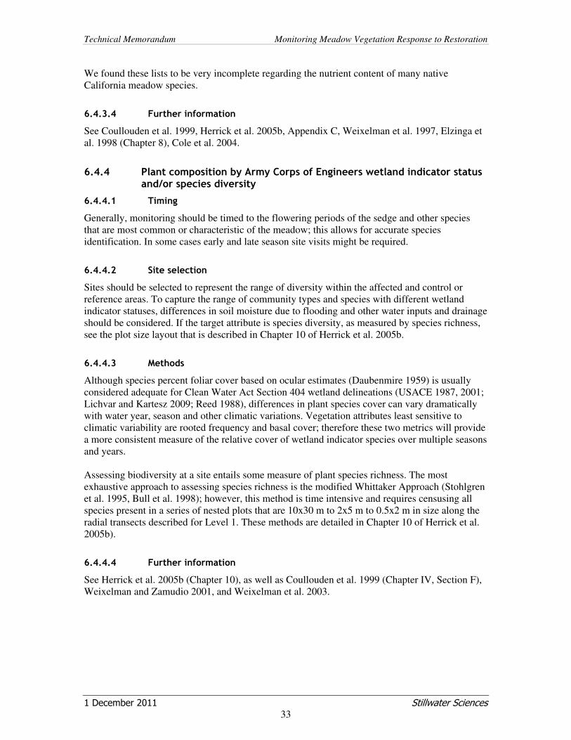
Technical Memorandum Monitoring Meadow Vegetation Response to Restoration
1 December 2011 Stillwater Sciences
33
We found these lists to be very incomplete regarding the nutrient content of many native California meadow species.
6.4.3.4 Further information
See Coullouden et al. 1999, Herrick et al. 2005b, Appendix C, Weixelman et al. 1997, Elzinga et al. 1998 (Chapter 8), Cole et al. 2004.
6.4.4 Plant composition by Army Corps of Engineers wetland indicator status and/or species diversity
6.4.4.1 Timing
Generally, monitoring should be timed to the flowering periods of the sedge and other species that are most common or characteristic of the meadow; this allows for accurate species identification. In some cases early and late season site visits might be required.
6.4.4.2 Site selection
Sites should be selected to represent the range of diversity within the affected and control or reference areas. To capture the range of community types and species with different wetland indicator statuses, differences in soil moisture due to flooding and other water inputs and drainage should be considered. If the target attribute is species diversity, as measured by species richness, see the plot size layout that is described in Chapter 10 of Herrick et al. 2005b.
6.4.4.3 Methods
Although species percent foliar cover based on ocular estimates (Daubenmire 1959) is usually considered adequate for Clean Water Act Section 404 wetland delineations (USACE 1987, 2001; Lichvar and Kartesz 2009; Reed 1988), differences in plant species cover can vary dramatically with water year, season and other climatic variations. Vegetation attributes least sensitive to climatic variability are rooted frequency and basal cover; therefore these two metrics will provide a more consistent measure of the relative cover of wetland indicator species over multiple seasons and years. Assessing biodiversity at a site entails some measure of plant species richness. The most exhaustive approach to assessing species richness is the modified Whittaker Approach (Stohlgren et al. 1995, Bull et al. 1998); however, this method is time intensive and requires censusing all species present in a series of nested plots that are 10x30 m to 2x5 m to 0.5x2 m in size along the radial transects described for Level 1. These methods are detailed in Chapter 10 of Herrick et al. 2005b).
6.4.4.4 Further information
See Herrick et al. 2005b (Chapter 10), as well as Coullouden et al. 1999 (Chapter IV, Section F), Weixelman and Zamudio 2001, and Weixelman et al. 2003.

Technical Memorandum Monitoring Meadow Vegetation Response to Restoration
1 December 2011 Stillwater Sciences
34
6.4.5 Floodplain vegetation sediment filtering and flood attenuation
6.4.5.1 Timing
Vegetation density within the floodplain, along with floodplain surface roughness and slope, affects on-site sediment filtering capacity and downstream flood attenuation. Sediment particles are captured on the floodplain when lateral flow velocity, which reflects the flood water’s capacity to carry particles, is reduced. Flow velocity is reduced with longer flow paths across the floodplain, lower slope, and increased friction. Surface roughness (e.g., boulders and topographic relief) and vegetation increase friction on flood waters, thereby increasing flood duration and sediment deposition. Therefore, vegetation attributes most directly tied to sediment filtering and flood attenuation are the lateral extent and density of vegetation in the flood prone area during flooding. Since flooding frequently occurs from snow melt through early summer (roughly May through June), measurements of vegetation density should be made during that period.
6.4.5.2 Site selection
Delineate the boundaries of the flood prone area within the restored/enhanced and control reaches of the meadow. Establish transects across the floodplain, perpendicular to the channel, that fall within the affected (restored/enhanced/protected) areas and an equal linear extent of transects that fall within the control (unaffected) area.
6.4.5.3 Methods
Establish a minimum of four transects per treatment, such that the range of dominant conditions are covered by these transects. Along each transect, measure vegetation cover, by species or to genus should be sufficient of these purposes. Daubenmire or Point Intercept methods, as described in Herrick et al. 2005a (QuickStart: Line-Point Intercept Method), Herrick et al. 2005b (Chapter 15: Quadrat-Point-Intercept), and Elzinga et al. 1998 (Chapter 8).
6.4.5.4 Further information
See Herrick et al. 2005a (QuickStart: Line-Point Intercept Method), Herrick et al. 2005b (Chapter 15: Quadrat-Point-Intercept), and Elzinga et al. 1998 (Chapter 8).
6.4.6 Fire effects on vegetation
6.4.6.1 Timing
For monitoring the effects (vs. risk) of fire, it is best to collect monitoring data during the same time of the growing season for both pre- and post-fire periods.
6.4.6.2 Site selection
Locating monitoring transects throughout the burned area, to capture the range of variability in burn intensity, should be a goal. Variation in burn intensity can be roughly estimated before the fire based on fuel load, surface and fuel (vegetation) moisture, and topography (Sugihara et al. 2006).
6.4.6.3 Methods
Many questions about meadow vegetation response to fire can be addressed by collecting pre- and post-fire data on species cover, richness, and tree (e.g., conifer, aspen) seedling density

Technical Memorandum Monitoring Meadow Vegetation Response to Restoration
1 December 2011 Stillwater Sciences
35
(Swanson et al. 2007). For species cover and richness, the line-point intercept method described in Herrick et al. 2005a (QuickStart: Line-Point Intercept Method) can be applied with the addition of collecting pre-burn data on fuel loading. A broader discussion of measuring species cover and richness is provided in Elzinga et al. 1998 (Chapter 8). Tree seedling recruitment rates pre- vs. post-burn can be collected using the Quadrat-Point Intercept method described in Herrick et al. 2005b (Chapter 15). For tree mortality data collection methods, see the next section on Meadow Edge Tree Dynamics.
6.4.6.4 Further information
Swanson et al. 2007, Haugo and Halpern 2007; Herrick et al. 2005a (QuickStart: Line-Point Intercept and Belt Transect Methods), Herrick et al. 2005b (Chapter 15: Quadrat-Point-Intercept, and Chapter 22: Fire), Elzinga et al. 1998 (Chapter 8); and other reports on conifer invasion of meadows (Helms 1987, Dunwiddie 1977, Arno and Gruell 1986, among others).
6.4.7 Edge tree dynamics
The authors located no existing protocols for monitoring meadow edge dynamics. Therefore, the following approach is provided as a suggestion, to be tailored to the site’s particular needs.
6.4.7.1 Timing
Begin monitoring as many seasons before treatment as possible and continue monitoring after treatment on an annual basis for the first 3 years. After this, monitoring can be less frequent, such as at 3 to 5 year intervals and, if possible, following events such as particularly wet or dry water years or fire.
6.4.7.2 Site selection
To monitor for tree encroachment into a meadow, permanent transects should be anchored at a point well within the adjacent forest where woody and herbaceous understory species reflect upland forest, rather than edge conditions. Each transect should then extend, perpendicular to the meadow edge, to a point well within the open meadow, where no forest or edge species are found. Along these transects, sampling can occur within a continuous (or intermittent) series of rectangular plots (6x3 m or 10 x 20 ft), situated with the long axis perpendicular to these transects. Transects should be established in areas where change is expected or has been observed and, if possible, in areas where no changes in tree density and composition have been observed or are expected.
6.4.7.3 Methods
Within each (or every other, depending on the resolution desired) rectangular plot, collect data on tree seedling density (number of seedlings per plot), tree species density (additional information could include tree size (dbh) and status [live/dead]), and percent cover of riparian shrubs, upland shrubs, forbs and graminoids. Ancillary measurements along these transects could also be collected and to improve understanding of observed dynamics; these include soil moisture, ground water level and litter thickness, among other possibilities. Comparisons of tree and seedling density as well as shrub and herbaceous cover along the transect and over time can be made using various statistical models to reveal relationships between changes in seedling density and other factors such as time, distance from the forest center, time since a change in management, flood, burn, or other event.

Technical Memorandum Monitoring Meadow Vegetation Response to Restoration
1 December 2011 Stillwater Sciences
36
6.4.7.4 Further information
See Swanson et al. 2007,Haugo and Halpern 2007, and Herrick et al. 2005b (Chapter 15: Quadrat-Point-Intercept, and Chapter 22: Fire), and Elzinga et al. 1998.
6.4.8 Special status species
6.4.8.1 Timing
The special-status plant species that are being monitored need to be assessed at an appropriate phenological stage, when the plant species is readily identifiable. Each year, an effort should be made to return to the site when the plants are at this same stage of development; this means adjusting the timing based on the water year type, average temperatures, etc. Monitoring should begin as many seasons before treatment as possible and continue after treatment on an annual basis for a minimum of three years. Ideally, there should also be a control that is not subjected to the treatment. After at least three consecutive years of monitoring (prior to treatment or using the control if necessary), field surveys results can be evaluated in order to develop a minimum acceptable threshold population size for each species. If treatment has already begun and management had no apparent effect on the species population sizes and extents as compared to the control, then surveys can be conducted less frequently (e.g., every five years) following completion of the baseline monitoring. If the change in meadow management coincided with significant changes in the species population during the first three years post-implementation, a monitoring plan can be devised that addresses potential sources of change (e.g., by targeting particular areas or conditions), including additional monitoring if necessary.
6.4.8.2 Site selection
If possible, include areas of the meadow that have been subject to change in management as well as areas that have not, as described for the BACI design (Smith 2002). Depending on the size of the population, a complete census may be appropriate or sub-sampling may be necessary. If a complete census is feasible, the sites will be selected based on the locations of the special-status plants. If a complete census is not feasible, a variety of methods of sub-sampling can be applied. However, generally speaking the site selection should capture enough of the population(s) to appropriately characterize the entire population(s). This may entail setting up multiple transects through one or individual populations, establishing a set number of quadrats, or delineating a search area parameter around more diffuse populations (standardized unit-effort [timed search] survey). For more detail, see methods below.
6.4.8.3 Methods
There are a variety of methods for assessing a special-status plant population through time. Characteristics of the plant species to monitored, such as size (tree versus herb) and life form (annual versus perennial) as well as the extent of the population (less than 100 individuals versus over 1,000 individuals) will determine the most appropriate sampling techniques. Quadrats of variable sizes, point intercept method, permanent belt transects, and standardized unit-effort (timed search) of the survey site are examples of methods that can be utilized, depending on the above. Quadrants of variable size and shape can be used to sample a population; decisions on dimensions are dependent upon features of the population such as the spatial distribution of species within the population (see Elzinga et al. 1998 for more information). The point intercept method entails estimating percent cover by recording the number of “hits” of each species at points along a transect. “Hits” are determined by vertically dropping a 0.25 in-diameter dowel,

Technical Memorandum Monitoring Meadow Vegetation Response to Restoration
1 December 2011 Stillwater Sciences
37
sharpened at the tip, at regular intervals along the transect; the first plant touched by the pointed tip was recorded as the “hit” for that point (Elzinga et al. 1998). Belt-line transects entail counting the number of plants per segment, each of which is made up of an appropriate-sized (e.g., 1x1 m) cell on both sides of the center line, and recording associated variables. The standardized unit-effort survey consists of one surveyor conducting a 60-minute timed search counting all individuals observed throughout the suitable habitat patch, with the timed search beginning once the first individual was located (USDA Forest Service 1999). Regardless of plot type, photographs should be taken and the following information types of information should be recorded:
• number of individuals;
• information on phenology (i.e., vegetatative, flowering, fruiting);
• signs of disturbance such as herbivory;
• canopy cover;
• plant community characteristics (e.g., dominant species and percent cover using modified Daubenmire [1959] cover class categories); and
• hydrologic characteristics and soil pH where applicable. Plant counts and plant condition should be recorded for each survey unit (e.g., each transect segment). Canopy cover and plant community characteristics can be recorded where there appeared to be a transition from one community type to another along a transect. The sampling frequency for other attributes, such as hydrologic characteristics and soil pH, can be adjusted based on the scale and variability within/amongst populations.
6.4.8.4 Further information
See Elzinga et al. 1998 and USDA Forest Service 1999.
6.4.9 Invasive Species
6.4.9.1 Timing
The targeted weed species that are being monitored need to be assessed at an appropriate phenological stage, when the plant species is readily identifiable. Prior to treatment (specifically of the weeds or of the site), a baseline assessment of the population extent (i.e., patch size, percent cover, and number of individuals) should be documented. After treatment, monitoring should continue on an annual basis. Depending on results of the survey (e.g., targeted species’ populations responding to treatment or population increasing in size), monitoring thereafter can be tailored in order to assess the overall effects of the treatment on weed species extent and distribution
6.4.9.2 Site selection
If possible, include areas of the meadow that will be subject to change in management as well as areas that will not, as described for the BACI design (Stewart-Oaten, Murdoch, and Parker 1986, Stewart-Oaten and Bence 2001, Underwood 1994, Smith 2002). Within these areas, if they are large and/or complex, prioritize those areas that support the most populations or greatest extent of the targeted weed populations.

Technical Memorandum Monitoring Meadow Vegetation Response to Restoration
1 December 2011 Stillwater Sciences
38
6.4.9.3 Methods
First, a list of priority or targeted weeds needs to be developed. A number of sources, including Cal IPC, CDFA, and the local USDA Forest Service office can provide information on weeds of concern. Once a list of priority weeds has been established and sites have been selected to monitor chosen populations, data on the extent of the population/ infestation needs to be recorded and compared through time. Data should be collected on sighting forms with the location and population boundaries recorded in the field using a GPS or mapped onto an orthophoto field base map. Information on the forms should include the following:
• Gross area of infestation (i.e., overall patch size);
• Percent cover;
• Weighted area of infestation (i.e., gross area multiplied by percent cover);
• Estimated number of individuals using, for example, the following abundance categories:
o Sparse (1–10 plants observed),
o Patchy (11–50 plants observed),
o Widespread (50–100 plants observed),
o Infested (100+ plants observed);
• Habitat description, including associated species and physical features of the site; and
• Phenology of the population. In the office, weed data should be uploaded into a GIS layer of point and/or polygon locations and attribute data should be entered into a database. This data can then be contributed to organizations tracking weeds locally (e.g., local USDA Forest Service district or National Park Service district) or throughout the state (e.g., California Early Detection Network), or even nationwide (NAWMA).
6.4.9.4 Further information
California Department of Food and Agriculture (CDFA) Plant Pest Diagnostics Center (http://www.cdfa.ca.gov/plant/PPD/botany_sampling.html); The Invasive Species Council of California (http://www.iscc.ca.gov/index.html), California Invasive Plant Council (Cal IPC; http://www.cal-ipc.org/), California Early Detection Network (http://californiaedn.org/), and the North American Weed Management Association (NAWMA; http://www.nawma.org/).
6.4.10 Riparian channel bank vegetation functions
Channel bank vegetation can perform several important functions. These include (1) shading the channel and thereby preventing additional warming which can negatively affect aquatic habitat; (2) stabilizing banks to prevent excessive erosion and sediment loading to the channel; and (3) providing in-channel coarse woody debris that create structural and habitat complexity for aquatic species. Riparian vegetation, particularly plant species with stoloniferous, rhizomatous, or other kinds of massive root structures, can stabilize channel banks and reduce sediment inputs. Plants such as Nebraska sedge and Geyer’s willow stabilize stream banks and slow flood waters by increasing floodplain roughness for flood waters (Winward 2000). Shading can be measured quite directly; however, direct measurement of the other functions is difficult and more frequently assessed using indirect measures.

Technical Memorandum Monitoring Meadow Vegetation Response to Restoration
1 December 2011 Stillwater Sciences
39
6.4.10.1 Timing
As described for other meadow characteristics, monitoring should begin at least one and preferably several years before the change in management, enhancement or restoration is implemented. It is generally best to monitor frequently following implementation (at least one time per year) in order to catch and correct or redirect any unexpected or undesired responses to the change. Although measurements of channel bank vegetation are not particularly sensitive to differences in timing during the growing season, the timing of these measurements should be kept consistent to minimize the confounding effects of plant phenology on classification of different meadow plant community types.
6.4.10.2 Site selection
Include areas of the meadow that will be subject to change in management as well as areas that will not be, as described for the BACI design ((Stewart-Oaten, Murdoch, and Parker 1986, Stewart-Oaten and Bence 2001, Underwood 1994, Smith 2002). Within these areas, if they are large and/or complex, prioritize those stream lengths that support the most common vegetation type along their green line (or bankfull position). The extent of community types along both sides of the bank will be measured.
6.4.10.3 Methods
Two completely different methodologies will be applied in order to monitor shade and bank stability. Channel Shade: The solar pathfinder ™ is a non-electronic and affordable (under $300) device that provides a fast and efficient means of determining changes in channel shade due to changes in riparian canopy cover; it can be used on any day at any time of day to determine light input during any time of the year or over the entire year. See Harris et al. 2005 and the solar pathfinder website (http://www.solarpathfinder.com/) for more detail. Bank Stability: Bank stability can be indirectly assessed and monitored based on the extent of different plant community types along the channel banks that have been subjected to a change in management or that are part of the control set. See Winward 2000 (Greenline) for more details.
6.4.10.4 Further information
See Coullouden et al. 1999, Elzinga et al. 1998, Harris et al. 2005, and Winward 2000.
6.4.11 Plant recruitment and survival
6.4.11.1 Timing
Begin monitoring as many seasons before treatment as possible and continue monitoring after treatment on an annual basis for the first 3 years. After this, monitoring can be less frequent, such as at 3- to 5-year intervals and, if possible, following events such as particularly wet or dry water years or fire.
6.4.11.2 Site selection
In cases where monitoring is to determine survival rates of installed plants, no control site or pre-implementation monitoring is necessary. However, permanent transects should be established within the actively planted area that reflects the range of variation in physical site conditions. If

Technical Memorandum Monitoring Meadow Vegetation Response to Restoration
1 December 2011 Stillwater Sciences
40
possible, establish permanent natural recruitment transects in areas of the meadow that will and will not be subject to the change in management.
6.4.11.3 Methods
Survival of installed plants can be measured using permanent transects in the actively planted area (see Elzinga et al. 1998, Coulloudren et al. 1999). Survival and vigor (e.g., height, percent of live foliage, etc.) of individual plants, located at a recorded point along each transect, can be surveyed at the end of each growing season. Naturally recruiting individuals within 1 meter to either side of the permanent transect can also be included and used to indicate recruitment rates as changes in density (transect length x 2 m) over time. See Winward 2000 (Woody Species Regeneration). Rules will need to be established on how to count multiple stemmed species, such as willow, as well as stoloniferous and rhizomatous species.
6.4.11.4 Further information
See Coullouden et al. 1999, Elzinga et al. 1998, and Winward 2000.
7 REPORTING AND SHARING FINDINGS
7.1 Monitoring Reports
As discussed in Section 5.7, reporting your findings is a critical step for all monitoring efforts. The process of organizing, describing, and interpreting your findings forces one to ferret out the important implications of the monitoring data—to be applied to improve management strategies and / or to adjust the monitoring program (see Figure 1 in Section 3.3). As described in Section 5.7, we recommend that monitoring reports be updated annually for at least the first three years following a major change in management and at five year intervals thereafter. Each year of monitoring data should be added into the previous report, so that the full history of monitoring and response is in a single document. Please refer to the general outline in Section 5.7 for guidance in the composition of Level 2 monitoring reports.
7.2 Sharing Findings in Monitoring Reports
Who should receive the monitoring reports? In many cases, you will need at least to submit reports to the funding source for the restoration project. However, it is generally beneficial to share findings in the monitoring reports (and the reports themselves) with a broader community of people and institutions involved in meadow restoration and management. In that way, we can all learn from each other’s accomplishments and challenges and meadow management in the Sierras can be done more effectively with fewer surprises. One way to make monitoring reports available to other interested parties is to post a PDF version of each annual updated report on a webpage for your host institution, ranch or funding agency. One can also make reports available in hard copy or other digital form (e.g., email attachment or CD) to local watershed groups, the local District office of the Forest Service, the local UC Agricultural Extension, local Resource Conservation District, and to local academic institutions.

Technical Memorandum Monitoring Meadow Vegetation Response to Restoration
1 December 2011 Stillwater Sciences
41
7.3 Data Storage and Data Sharing
Once data have been collected, summarized and analyzed, do not discard the source data files (e.g., excel or access). These source data files should be kept in a well-placed and named folder so that they can be found and retrieved easily. When computers are replaced, these data files should be moved onto the new hard drives (which are backed up frequently in case of hard disk-damaging power surges, etc.). In addition to storing data within the home institution that performed the restoration and monitoring, there have been multiple calls for a publically available website that is maintained by permanent (likely part-time) staff, to house information on meadow condition, restoration, and monitoring in a spatially explicit and retrievable manner. We are hopeful that such website will be created, along with long-term funding to sustain it, such that it can be searched for documents and accompanying data using web-based software.

Technical Memorandum Monitoring Meadow Vegetation Response to Restoration
1 December 2011 Stillwater Sciences
42
8 LITERATURE CITED
American Rivers and others. 2011. Monitoring protocol for hydrology and water quality response to restoration of meadows in the Sierra Nevada. Prepared by American Rivers for National Fish and Wildlife Foundation. Available at: http://www.americanrivers.org/MeadowPubs Arno, S. F. and Gruell, G. E. 1986. Douglas-fir encroachment into mountain grasslands in southwestern Montana. Journal of Range Management 39: 272–276. Bombay, H. L., G. A. Green, M. L. Morrison. 2003. Conservation assessment of the willow flycatcher in the Sierra Nevada. Bull, K., K. W. Stolte, and T.J. Stohlgren. 1998. Forest Health Monitoring: Vegetation Pilot Field Methods Guide. USDA, Forest Service. Washington, DC. Cayan, D. R., S. Kammerdiener, M. D. Dettinger, J. M. Caprio, and D. H. Peterson. 2001. Changes in the onset of spring in the western United States. Bulletin of the American Metrological Society 82: 399–415. Chambers, J. C., and A. R. Linnerooth. Restoring riparian meadows currently dominated by Artemisia using alternative state concepts—the establishment component. Applied Vegetation Science 4: 157–166. CNPS 2011. California Native Plant Society and Department of Fish and Game protocol for combined vegetation rapid assessment and releve sampling field form. May 13, 2011. (http://www.cnps.org/cnps/vegetation/pdf/protocol-combined.pdf).
CNPS (California Native Plant Society) Vegetation Committee. 2004. California Native Plant Society vegetation rapid assessment protocol (November 5, 2001, revised September 20, 2004). Prepared by the CNPS Vegetation Committee, Sacramento, California. CNPS (California Native Plant Society). 2001. Inventory of Rare and Endangered Plants of California (sixth edition). Rare Plant Scientific Advisory Committee, David P. Tibor, Convening Editor. California Native Plant Society. Sacramento, CA. 388 pp. (7th Edition available only in electronic form at: http://cnps.site.aplus.net/cgi-bin/inv/inventory.cgi) Coffman, G. C. 2007. Factors Influencing Invasion of Giant Reed (Arundo donax) in Riparian Ecosystems of Mediterranean-type Climate Regions. Dissertation, University of California, Los Angeles, California. Cole, David N., J. W. Van Wagtendonk, M. P. McClaran, P. E. Moore, and N. K. McDougald. 2004. Response of mountain meadows to grazing by recreational packstock. Journal of Range Management 57: 153–160. Coles-Ritchie, M. C., A. Kelly, and R. Henderson. PIBO Riparian Vegetation Sampling 2004. Protocol available at: www.fs.fed.us/biology/fishecology/emp/. Coulloudon, W., K. Eshelman, J. Gianola, N. Habich, L. Hughes, C. Johnson, M. Pellant, P. Podborny, A. Rasmussen, B. Robles, P. Shaver, J. Spehar, J. Willoughby. 1999. Sampling

Technical Memorandum Monitoring Meadow Vegetation Response to Restoration
1 December 2011 Stillwater Sciences
43
vegetation attributes: interagency technical reference. Cooperative Extension Service, USDA Forest Service, Natural Resource Conservation Service, Grazing Land Technology Institute, Bureau of Land Management. 1996 Revised in 1997, and 1999. Technical Reference 1734-4 http://www.blm.gov/nstc/library/pdf/samplveg.pdf. Craig, D. and P. L. Williams. 1998. Willow Flycatcher (Empidonax traillii). In The riparian bird conservation plan: a strategy for reversing the decline of riparian-associated birds in California. CDWR (California Department of Water Resources). 2011. Delta levees maintenance subventions program guidelines: procedures and criteria. Adopted by Central Valley Flood Protection Board (September 23, 2011). Prepared by the Delta Levees and Environmental Engineering Branch of DWR. Doubt, J. C. and R. J. Belland. 2000. Monitoring Protocols for Elements of Non-vascular Plant Diversity in Alberta's Forested Zones. Alberta Research Council, Alberta Biodiversity Monitoring Institute, Vegreville, Alberta, Canada. Dunne, T., L.B. Leopold. 1978. Water in environmental planning. W.H. Freeman and Company. ISBN 0-7167-0079-4. Dunwiddie, P. W. 1977. Recent tree invasion of subalpine meadows in the Wind River Mountains, Wyoming. Arctic and Alpine Research 9: 393–399. Elzinga, C., D. W. Salzer, J. W. Willoughby. 1998. Measuring and monitoring plant populations. BLM Technical Reference 1730-1 BLM/RS/ST-98/005+1730. http://www.blm.gov/nstc/library/pdf/MeasAndMon.pdf. Feather CRM. 2010. Quantification of carbon sequestration benefits of restoring degraded montane meadows: Technical Report. Available at: http://www.feather-river-crm.org/index.php?option=com_content&view=article&id=63&Itemid=63. Harris, R. R., S. D. Kocher, J. M. Gerstein and C. Olson. 2005. monitoring the effectiveness of riparian vegetation restoration. Center for Forestry, University of California, Berkeley. Haugo, R. D. and C. P. Halpern. 2007. Vegetation responses to conifer encroachment in a western Cascade meadow: a chronosequence approach. Canadian Journal of Botany. 85: 285-198. Helms, J. A. 1987. Invasion of Pinus contorta var. murrayana into mountain meadows at Yosemite National Park., California. Madrono 34: 91–97. Herrick, J. E., J. W. Van Zee, K. M. Havstad, L. M. Burkett, and W. G. Whitford. 2005a. Monitoring manual for grassland, shrubland and savanna ecosystems. Volume 1: Quick Start. USDA-ARS Jornada Experimental Range. ISBN 0-9755552-0-0. (www.uapress.arizona.edu). Herrick, J.E., J.W. Van Zee, K. M. Havstad, L.M. Burkett, and W. G. Whitford. 2005b. Monitoring manual for grassland, shrubland and savanna ecosystems. Volume II: Design, supplementary methods and interpretation. USDA-ARS Jornada Experimental Range. ISBN 0-9755552-0-0. (www.uapress.arizona.edu). Hickman, J. C., editor. 1993. The Jepson manual, higher plants of California. University of California Press, Berkeley, California.

Technical Memorandum Monitoring Meadow Vegetation Response to Restoration
1 December 2011 Stillwater Sciences
44
ICF Jones & Stokes. 2008. Plumas watershed forum program review. Consultant’s Report. Prepared for Plumas County Flood Control and Water Conservation District. Lichvar, R. W. and J. T. Kartesz. 2009. North American digital flora: national wetland plant list, version 2.4.0 (https://wetland_plants.usace.army.mil). U.S. Army Corps of Engineers, Engineer Research and Development Center, Cold Regions Research and Engineering Laboratory, Hanover, New Hampshire, and BONAP, Chapel Hill, North Carolina.
Menke, J. W., C. Davis, P. Beesley. 1996. Public rangeland/livestock grazing assessment. Chapter 22 in Sierra Nevada Ecosystem Project, Final report to Congress. Vol. III. Available at: http://pubs.usgs.gov/dds/dds-43/VOL III/VIII C22.PDF Micheli, E.R. and J.W. Kirchner. 2002a. Effects of wet meadow riparian vegetation on streambank erosion. 2. Measurements of vegetated bank strength and consequences for failure mechanics. Earth Surface Processes and Landforms 27: 687–697.
Micheli, E. R., and J. W. Kirchner. 2002b. Effects of wet meadow riparian vegetation on streambank erosion. 1. Remote sensing measurements on streambank migration and erodibility. Earth Surface Processes and Landforms 27: 627–639.
Mote, P. W. 2006. Climate-Driven Variability and Trends in Mountain Snowpack in Western North America. Journal of Climate. Volume 19. pp. 6209-6220 National Riparian Service Team. 2004. Riparian Vegetation Monitoring Protocol Meeting. Logan, Utah. September 21-23, 2004. Prineville, Oregon. (http://www.or.blm.gov/nrst) Pellant, M., P. Shaver, D.A. Pyke, and J.E. Herrick. 2005. Interpreting indicators of rangeland health, version 4. Technical Reference 1734-6. U.S. Department of the Interior, Bureau of Land Management, National Science and Technology Center, Denver, CO. BLM/WO/ST-00/001+1734/REV05. 122 pp. Potter, D.A. 2005. Riparian Plant Community Classification; west slope, central and southern Sierra Nevada, California. USDA Forest Service, Pacific Southwest Region. R5-TP-022. Ratliff. R. D. 1985. Meadows in the Sierra Nevada of California: state of knowledge. Gen. Tech. Rep. PSW-84. Berkeley, California. Pacific Southwest Forest and Range Experiment Station, Forest Service, U.S. Department of Agriculture. Albany, California. Reed, P.B. 1988. National list of plant species that occur in wetlands: 1988 national summary. National Wetland Inventory, U.S. Fish and Wildlife Service. http://wetlands.fws.gov/plants.htm Rosatti, F. J. 2003. Jepson online interchange for California floristics. Fremonita 31: 23–30. Sawyer, J. O., T. Keeler-Wolf, and J. M. Evans. 2009. A manual of California vegetation, 2nd Edition. California Native Plant Society in collaboration with California Department of Fish and Game, Sacramento, California.
Schlesinger, W. H. 1997. Biogeochemistry: An analysis of global change. 2nd Edition. Academic Press, San Diego, California.

Technical Memorandum Monitoring Meadow Vegetation Response to Restoration
1 December 2011 Stillwater Sciences
45
Smith, E. P. 2002. BACI design. Volume 1, pp. 141-148 in Encyclopedia of Environmetrics (ISBN 0471 899976). El-Shaarawi, Abdel H. and W. W. Piegorsch, Editors. John Wiley & Sons, Ltd. Chichester, UK. Stohlgren. T.JM.B. Falkner, and L.D. Schell. 1995. A modified Whittaker nested vegetation sampling method. Vegetation. 117:113-121. Stewart-Oaten, A., W.W. Murdoch, K.R. Parker. 1986. Environmental impact assessment: "pseudoreplication" in time? Ecology 67(4):929-940. Stewart-Oaten, A., and JR Bence. 2001. Temporal and spatial variation in environmental impact assessment. Ecological Monographs 71:305-339. Sugihara, N.G., J. W. Van Wagtendonk, K.E. Shaffer, J. Fites-Kaufman, A.E. Thode. 2006. Fire in California’s Ecosystems. University of California Press. Berkeley, CA. Swanson, F. J., C. B. Halpern, J. H. Cissel. 2007. Restoration of dry, montane meadows through prescribed fire, vegetation and fuels management: A program of research and adaptive management in western Oregon. Project 01C-3-3-10. Final Report to the Joint Fire Science Program. Underwood, A. J. 1994. On beyond BACI: sampling designs that might reliably detect environmental disturbances. Ecological Applications 4:3-15. USACE (Army Corps of Engineers). 1987. Corps of Engineers wetlands delineation manual. Technical Report Y-87-l. U.S. Army Engineer Waterways Experiment Station, Vicksburg, Mississippi. USACE. 2001. Minimum standards for acceptance of preliminary wetland delineations. Advisory letter from District Chief Art Champ. www.spk.usace.army.mil/pub/outgoing /co/regwldet01.pdf USDA Forest Service. 1999. Forest health monitoring 1999 field methods guide. USDA Forest Service, National Forest Health Monitoring Program, Research Triangle Park, North Carolina. Weixelman, D.A., B.Hill, D.J. Cooper, E.L.Berlow, J.H. Viers, S.E. Purdy, A.G. Merrill, S.E. Gross. 2011. A field key to meadow hydrogeomorphic types for the Sierra Nevada and southern Cascade Ranges in California. Gen. Tech.Rep. USDA Forest Service, Pacific Southwest Region. Vallejo, California. Weixelman, D., G. Bakker, and J. Fites. 2003. USFS Region 5 Range Monitoring Project 2003 Report. Adaptive Management Services, U.S. Forest Service, Nevada City, California. Weixelman, D., and D. Zamudo. 2001. Field Methods for Rooted Frequency Vegetation and Soil Quality Trend Sampling of Riparian Ecological Sites in Meadows, USDA Forest Service, California Rangeland Interagency Video Series: A Frequency Method. Weixelman, D.A., D. C. Zamudio, K.A. Zamudio, and R. J. Tausch. 1997. Classifying ecological types and evaluating site degradation in riparian areas. Journal of Range Management 50: 315-321.

Technical Memorandum Monitoring Meadow Vegetation Response to Restoration
1 December 2011 Stillwater Sciences
46
Winward, Alma H. 2000. Monitoring the vegetation resources in riparian areas. Gen. Tech. Rep. RMRS-GTR-47. Ogden, UT: U.S. Department of Agriculture, Forest Service, Rocky Mountain Research Station. (http://www.or.blm.gov/nrst/Tech_References/tech_references.htm).

Appendices

Appendix A
Level 1 Field Data Sheets

Technical Memorandum Monitoring Meadow Vegetation Response to Restoration
1 December 2011 Stillwater Sciences
A-1
Plant Community Type Plots: Descriptive Information
Page of
Date:
Project Name/No:
Meadow Name: Meadow ID:
Meadow Number: Crew Members:
General comments:
Aerial Photo Number with notes:
Other photo numbers and descriptions
Vegetation Descriptions per Plant Community Type
Com
munity T
ype
Code
Poly
gon n
um
ber
Tota
l V
egeta
tion
Sedge a
nd r
ush
specie
s
Oth
er
Gra
min
oid
s
Forb
s
Shru
bs
Tre
es (
not
seedlin
gs)
Tre
e s
eedlin
gs
Bare
min
era
l soil
Bare
org
anic
soil
Rock
Litte
r
Rooting D
ensity
Satu
rate
d
soil/
sta
ndin
g w
ate
rNotes
Absolute Percent Cover

Technical Memorandum Monitoring Meadow Vegetation Response to Restoration
1 December 2011 Stillwater Sciences
A-2
Plant Community Type Plot: Plant Species List with Percent Cover
Page of
Date:
Project Name/No:
Meadow Name: Meadow ID:
Meadow Number: Crew Members:
Plant Species list
Co
mm
un
ity
Ty
pe
Co
de
Po
lyg
on
nu
mb
er
Sp
ec
ime
n
co
lle
cte
d?
Scientific name Common name Layer
Percent
cover
(absolute)

Appendix B
Data Entry Forms
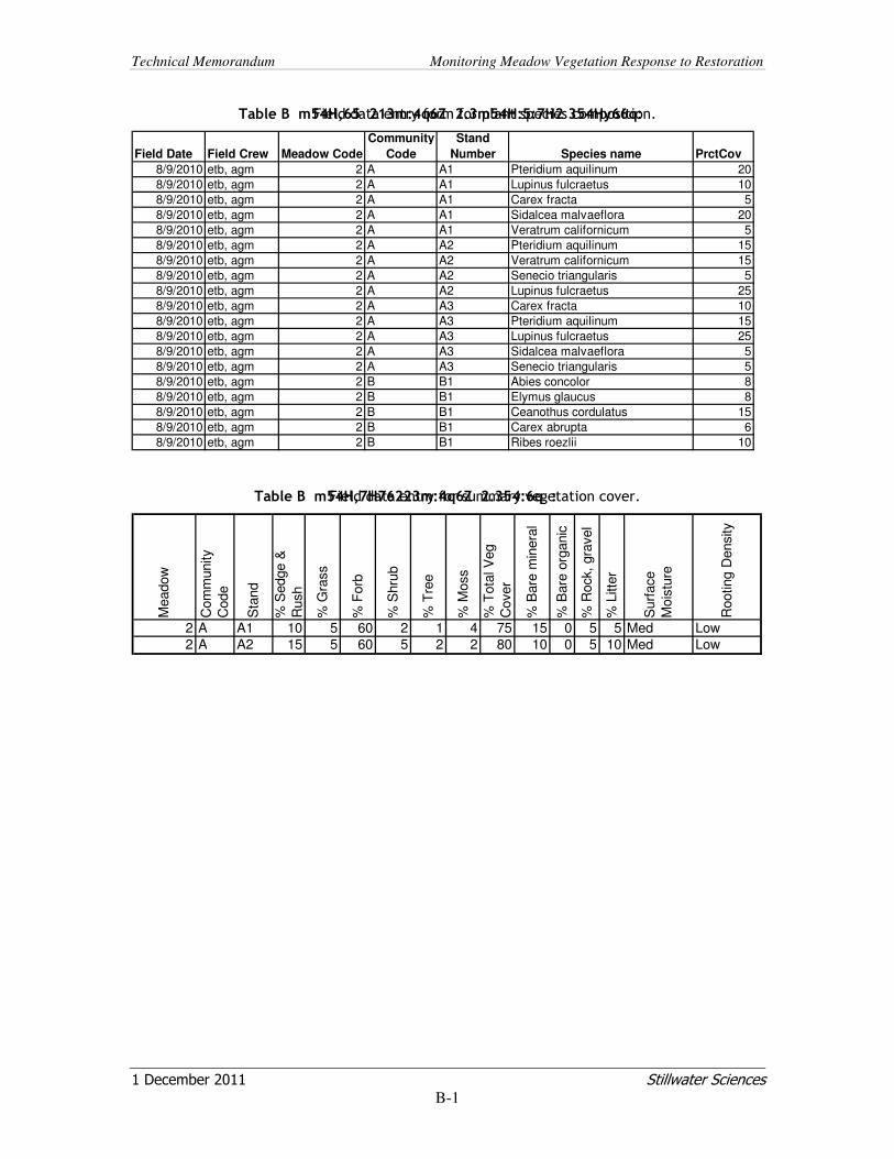
Technical Memorandum Monitoring Meadow Vegetation Response to Restoration
1 December 2011 Stillwater Sciences
B-1
Table B 1. Field data entry form for plant species composition.
Field Date Field Crew Meadow Code
Community
Code
Stand
Number Species name PrctCov
8/9/2010 etb, agm 2 A A1 Pteridium aquilinum 20
8/9/2010 etb, agm 2 A A1 Lupinus fulcraetus 10
8/9/2010 etb, agm 2 A A1 Carex fracta 5
8/9/2010 etb, agm 2 A A1 Sidalcea malvaeflora 20
8/9/2010 etb, agm 2 A A1 Veratrum californicum 5
8/9/2010 etb, agm 2 A A2 Pteridium aquilinum 15
8/9/2010 etb, agm 2 A A2 Veratrum californicum 15
8/9/2010 etb, agm 2 A A2 Senecio triangularis 5
8/9/2010 etb, agm 2 A A2 Lupinus fulcraetus 25
8/9/2010 etb, agm 2 A A3 Carex fracta 10
8/9/2010 etb, agm 2 A A3 Pteridium aquilinum 15
8/9/2010 etb, agm 2 A A3 Lupinus fulcraetus 25
8/9/2010 etb, agm 2 A A3 Sidalcea malvaeflora 5
8/9/2010 etb, agm 2 A A3 Senecio triangularis 5
8/9/2010 etb, agm 2 B B1 Abies concolor 8
8/9/2010 etb, agm 2 B B1 Elymus glaucus 8
8/9/2010 etb, agm 2 B B1 Ceanothus cordulatus 15
8/9/2010 etb, agm 2 B B1 Carex abrupta 6
8/9/2010 etb, agm 2 B B1 Ribes roezlii 10
Table B 2. Field data entry for summary vegetation cover.
Meadow
Com
munity
Code
Sta
nd
% S
edge &
Rush
% G
rass
% F
orb
% S
hru
b
% T
ree
% M
oss
% T
ota
l V
eg
Cover
% B
are
min
era
l
% B
are
org
anic
% R
ock,
gra
vel
% L
itte
r
Surf
ace
Mois
ture
Rooting D
ensity
2 A A1 10 5 60 2 1 4 75 15 0 5 5 Med Low
2 A A2 15 5 60 5 2 2 80 10 0 5 10 Med Low

Appendix C
Forage Nutrient Content Sampling and Analysis
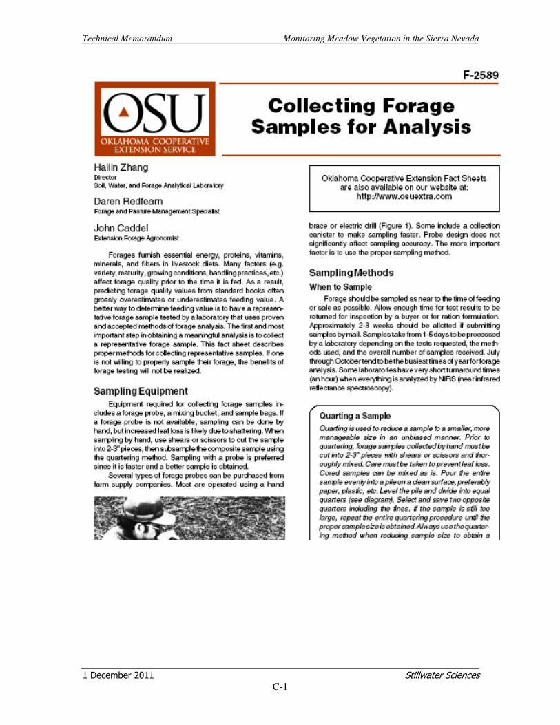
Technical Memorandum Monitoring Meadow Vegetation in the Sierra Nevada
1 December 2011 Stillwater Sciences
C-1

Technical Memorandum Monitoring Meadow Vegetation in the Sierra Nevada
1 December 2011 Stillwater Sciences
C-2
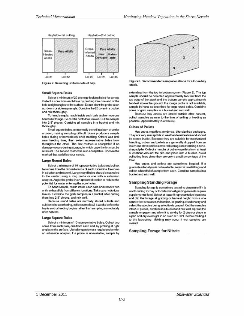
Technical Memorandum Monitoring Meadow Vegetation in the Sierra Nevada
1 December 2011 Stillwater Sciences
C-3

Technical Memorandum Monitoring Meadow Vegetation in the Sierra Nevada
1 December 2011 Stillwater Sciences
C-4
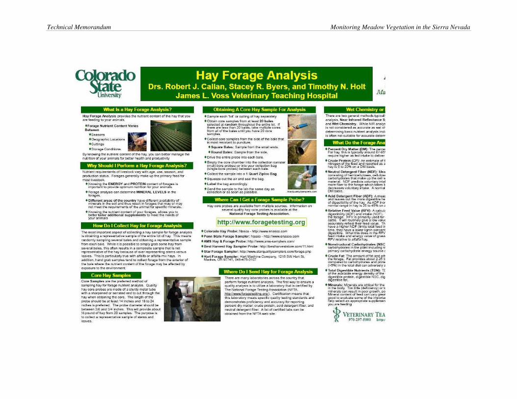
Technical Memorandum Monitoring Meadow Vegetation in the Sierra Nevada

Appendix D
List of Common Meadow Plant Species with Wetland
Indicator Status and USFS R5 Functional Group Information

Technical Memorandum Monitoring Meadow Vegetation in the Sierra Nevada
1 December 2011 Stillwater Sciences
D-1
SP
EC
IES
SC
IEN
TIF
IC N
AM
E
WE
TL
AN
D
WE
T
MO
IST
DR
Y
FU
NC
TIO
N
N F
IXE
R
GR
AS
S
GR
AS
SL
IKE
FO
RB
WO
OD
Y
LIF
EH
IST
RO
OT
HT
LA
TE
RA
LS
ABCO Abies contorta APL E E E WOODYDRY 0 0 0 0 1 2 10 100 2
ABMA Abies magnfica FACU E E E woodydry 0 0 0 0 1 2 15 100 2
ACMI2 Achillea millefolium FACU E E E rhizforbdry 0 0 0 1 0 2 15 4 4
ACHNA Achnatherum FACU E M L gramupl 0 1 0 0 0 2 10 5 2
ACLE Achnatherum lettermanii FACU E M L gramupl 0 1 0 0 0 2 4 5 2
ACLE8 Achnatherum lettermanii FACU E M L gramupl 0 1 0 0 0 2 4 5 2
ACLE9 Achnatherum lettermanii FACU E E L gramupl 0 1 0 0 0 2 12
ACNE9 Achnatherum nelsonii UPL E M L gramupl 0 1 0 0 0 2 7 5 2
ACCO4 Aconitum columbianum FACW L L L taprootwet 0 0 0 1 0 2 18 5 2
AGAU2 Agoseris aurantiaca FACU E M M taprootdry 0 0 0 1 0 2 11 4 2
AGGL Agoseris glauca FACU E E E taprootdry 0 0 0 1 0 2 5 4 2
AGGR AGOSERIS GRANDIFLORA FAC E E E taprootdry 0 0 0 1 0 2 7 4 2
AGHE2 Agoseris heterophylla FAC E E E taprootdry 0 0 0 1 0 1 8 4 1
AGOSE Agoseris sp. FAC E E E taprootdry 0 0 0 1 0 2 13 4 2
AGIN2 AGROPYRON INTERMEDIUM UPL E E E gramdry 0 1 0 0 0 2 4 3 4
AGEX Agrostis exarata FACW E E L gramshallow 0 1 0 0 0 2 14 4 4
AGGI2 Agrostis gigantea FAC E E M gramshallow 0 1 0 0 0 2 12 4 4
AGHA2 Agrostis hallii FACW E E E gramshallow 0 1 0 0 0 2 5 4 5
AGTH2 Agrostis humilis FACW M M L gramshallow 0 1 0 0 0 2 14 4 4
AGID Agrostis idahoensis FACW L L L gramshallow 0 1 0 0 0 2 24 4 3
AGOR Agrostis oregonensis FACW L L L gramshallow 0 1 0 0 0 2 11 4 2
AGDI Agrostis pallens FACW L L L gramshallow 0 1 0 0 0 2 14 4 4
AGPA8 Agrostis pallens FACW L L L gramshallow 0 1 0 0 0 2 14 4 4
AGSC Agrostis scabra FAC E E E gramshallow 0 1 0 0 0 2 19 4 3
AGSC5 Agrostis scabra FAC E E E gramshallow 0 1 0 0 0 2 19 4 3
AGROS Agrostis sp. FAC E E L gramshallow 0 1 0 0 0 2 20 4 2
AGST Agrostis stolonifera FACW E E E gramshallow 0 1 0 0 0 2 15 4 5
AGST2 Agrostis stolonifera FACW E E E gramshallow 0 1 0 0 0 2 15 4 5
AGST8 Agrostis stolonifera FACW E E E gramshallow 0 1 0 0 0 2 13 4 5
AGTH Agrostis thurberiana OBL M M L gramshallow 0 1 0 0 0 2 12
AGVA Agrostis variabilis FACW L L L gramshallow 0 1 0 0 0 2 10 4 4
AICA Aira caryophyllea FAC E E E annual 0 1 0 0 0 1 1 4 1
AIRA Aira sp. FAC E E E annual 0 1 0 0 0 1 1 4 1
ALLIU Allium sp. FAC L L M taprootdry 0 0 0 1 0 2 9 4 3
ALAE Alopecurus aequalis OBL E E E gramshallow 0 1 0 0 0 2 8 5 2
ALOPE Alopecurus sp. FAC E E L gramshallow 0 1 0 0 0 2 8 5 2
AMPS Ambrosia psilostachya FACU E E E taprootdry 0 0 0 1 0 1 6 4 1
ANAR Anagallis arvensis FAC E E E taprootdry 0 0 0 1 0 1 6 2 1
ANDE3 ANEMONE DELTOIDEAE UPL E E E taprootdry 0 0 0 1 0 2 3 1 2
ANCA10 ANEMOPSIS CALIFORNICA OBL M M M rhizforbwet 0 0 0 1 0 2 4 1.5 4
ANCO Antennaria corymbosa FAC E E M taprootdry 0 0 0 1 0 2 8 3 3

Technical Memorandum Monitoring Meadow Vegetation in the Sierra Nevada
1 December 2011 Stillwater Sciences
D-2
SP
EC
IES
SC
IEN
TIF
IC N
AM
E
WE
TL
AN
D
WE
T
MO
IST
DR
Y
FU
NC
TIO
N
N F
IXE
R
GR
AS
S
GR
AS
SL
IKE
FO
RB
WO
OD
Y
LIF
EH
IST
RO
OT
HT
LA
TE
RA
LS
ANDI2 Antennaria dimorpha FAC E E M taprootdry 0 0 0 1 0 2 12 3 3
ANME2 Antennaria media FAC E E M taprootdry 0 0 0 1 0 2 10 3 3
ANRO2 Antennaria rosea FAC E E E taprootdry 0 0 0 1 0 2 8 3 3
ANTEN Antennaria sp. FAC E E M taprootdry 0 0 0 1 0 2 6 3 3
ANTENNARIA Antennaria sp. FAC E E M taprootdry 0 0 0 1 0 2 8 3 3
ARABI Arabis sp. FAC E E M taprootdry 0 0 0 1 0 2 6 3 2
ARENA Arenaria sp. FAC E E M taprootdry 0 0 0 1 0 2 6 3 3
ARAM2 Arnica amplexicaulis FAC E E M rhizforbdry 0 0 0 1 0 2 17 4 5
ARCH3 ARNICA CHAMISSONIS FAC E E M rhizforbdry 0 0 0 1 0 2 16 4 5
ARCHF ARNICA CHAMISSONIS FAC E E M rhizforbdry 0 0 0 1 0 2 16 4 5
ARLO6 Arnica longifolia FACW M M M rhizforbwet 0 0 0 1 0 2 12 4 5
ARMO Arnica mollis FACW M M M rhizforbwet 0 0 0 1 0 2 9 4 5
ARMO4 Arnica mollis FACW M M M rhizforbwet 0 0 0 1 0 2 9 4 5
ARMO4 Arnica mollis FACW M M M rhizforbwet 0 0 0 1 0 2 9 4 5
ARNE3 ARNICA NEVADENSIS UPL E E E rhizforbdry 0 0 0 1 0 2 12 4 5
ARSO2 ARNICA SORORIA UPL E E E taprootdry
ARNIC Arnica sp. FAC M M M rhizforbdry 0 0 0 1 0 2 12 4 5
ARTRT Artemesia tridentata FACU E E E taprootdry 0 0 0 1 0 2 5 5 3
ARCA13 Artemisia cana FAC E E M rhizforbdry 0 0 0 1 0 2 16 4 5
ARDO3 Artemisia douglasiana FAC E M M taprootdry 0 0 0 1 0 2 5 4 3
ARLU Artemisia ludoviciana FACU E E E rhizforbdry 0 0 0 1 0 2 5 4 4
ARTEM ARTEMISIA SP. FACU E E E taprootdry 0 0 0 1 1 2 3 6 3
ARTR2 ARTEMISIA TRIDENTATA FACU E E E taprootdry 0 0 0 1 1 2 3 6 3
ARTRV Artemisia tridentata vaseyana FACU E E E taprootdry 0 0 0 1 1 2 1 6 3
ASAL Aster alpigenus ssp. andersonii FACW M M M rhizforbwet 0 0 0 1 0 2 12 1 4
ASAL2 Aster alpigenus ssp. andersonii FACW M M M rhizforbwet 0 0 0 1 0 2 12 1 4
ASALA Aster alpigenus ssp. andersonii FACW M M M rhizforbwet 0 0 0 1 0 2 14 4 4
ASALA2 Aster alpigenus ssp. andersonii FACW M M M rhizforbwet 0 0 0 1 0 2 12 1 4
ASALA3 Aster alpigenus ssp. andersonii FACW M M M rhizforbwet 0 0 0 1 0 2 12 1 4
ASFO Aster foliaceous FAC E E E rhizforbdry 0 0 0 1 0 2 16 4 4
ASOC Aster occidentalis FAC E E E rhizforbdry 0 0 0 1 0 2 14 4 4
ASTER ASTER SP. FAC E E E rhizforbdry 0 0 0 1 0 2 12 4 4
BOCR Botrychium crenulatum FAC L L L taprootdry 0 0 0 1 0 2 13 2 2
BOPI Botrychium PINNATUM FAC L L L taprootdry 0 0 0 1 0 2 19 2 2
BOSI Botrychium simplex FAC L L L taprootdry 0 0 0 1 0 2 19 2 2
BOTRY Botrychium SP. FAC L L L taprootdry 0 0 0 1 0 2 19 2 2
BRASS Brassica sp. FAC E E M taprootdry 0 0 0 1 0 2 12 4 2
BRODI Brodiaea sp. FAC E E M taprootdry 0 0 0 1 0 2 12 4 3
BRCA5 Bromus carinatus FAC E M L gramupl 0 1 0 0 0 2 8 5 2
BRDI3 BROMUS DIANDRUS UPL E E E annual 0 1 0 0 0 1 0 2 1
BRHO2 BROMUS HORDACEOUS UPL E E E annual
BRIN2 Bromus inermis FAC E E M gramupl 0 1 0 0 0 2 6 5 5
BRJA BROMUS JAPONICUS FACU E E E annual 0 1 0 0 0 1 1 1 1
BRMA BROMUS MADRITENSIS UPL E E E annual
BROMUS BROMUS SP. FACU E M L gramupl
BRSU2 Bromus suksdorfii FAC E M L gramupl 0 1 0 0 0 2 8 5 2
BRTE Bromus tectorum UPL E E E gramupl 0 1 0 0 0 1 1 4 1
CACA4 Calamagrostis canadensis FACW L L L gramdeep 0 1 0 0 0 2 15 5 4

Technical Memorandum Monitoring Meadow Vegetation in the Sierra Nevada
1 December 2011 Stillwater Sciences
D-3
SP
EC
IES
SC
IEN
TIF
IC N
AM
E
WE
TL
AN
D
WE
T
MO
IST
DR
Y
FU
NC
TIO
N
N F
IXE
R
GR
AS
S
GR
AS
SL
IKE
FO
RB
WO
OD
Y
LIF
EH
IST
RO
OT
HT
LA
TE
RA
LS
CAUM2 Calyptridium umbellatum UPL E E E taprootdry 0 0 0 1 0 2 2 1 2
CALAM CAMAGROSTIS SP. FAC L L L gramdeep
CAQU2 Camassia quamash FACW L L L taprootwet 0 0 0 1 0 2 22 4 2
CARDU Carduus sp. FACU E E taprootdry 0 0 0 1 0 2 3 4 2
CAAB Carex abrupta FACW L L L gramdeep 0 0 1 0 0 2 16 4 3
CAAQ Carex aquatilis OBL L L L gramdeep 0 0 1 0 0 2 25 5 3
CASI3 Carex aquatilis OBL L L L gramdeep 0 0 1 0 0 2 25 5 3
CAAT3 Carex athrostachya FACW L L L gramdeep 0 0 1 0 0 2 17 4 3
CAAU Carex aurea OBL L L L gramdeep 0 0 1 0 0 2 16 3 4
CAAU3 Carex aurea OBL L L L gramdeep 0 0 1 0 0 2 16 3 4
CABO2 Carex bolanderi FACW L L L gramshallow 0 0 1 0 0 2 13 4 3
CACA13 Carex capitata OBL L L L gramdeep 0 0 1 0 0 2 36 3 3
CADE8 Carex densa OBL L L L gramdeep 0 0 1 0 0 2 15 4 3
CADO Carex douglasii FACU E M M gramupl 0 0 1 0 0 2 12 3 4
CADO2 Carex douglasii FACU E M M gramupl 0 0 1 0 0 2 12 3 4
CAEC Carex echinata OBL L L L gramdeep 0 0 1 0 0 2 39 4 3
CAECE Carex echinata ssp. echinata OBL L L L gramdeep 0 0 1 0 0 2 17 4 3
CAEL2 CAREX ELEOCHARIS OBL L L L gramdeep 0 0 1 0 0 2 17 4 3
CAFE4 Carex feta OBL L L L gramshallow 0 0 1 0 0 2 11 5 3
CAFI Carex filofolia FACW L L L gramshallow 0 0 1 0 0 2 9 4 3
CAFI2 Carex fissuricola FACW L L L gramdeep 0 0 1 0 0 2 15 5 3
CAHE8 Carex heteroneura FACW L L L gramdeep 0 0 1 0 0 2 15 5 3
CAIL Carex illota OBL L L L gamdeep 0 0 1 0 0 2 15 5 3
CAIN10 Carex integra FACW L L L gramdeep 0 0 1 0 0 2 17 4 3
CAJO Carex jonesii FACW L L L gramdeep 0 0 1 0 0 2 17 4 5
CALA30 Carex lanuginosa OBL L L L gramdeep 0 0 1 0 0 2 22 5 5
CALE6 CAREX LEAVENWORTHII FACW L L L taprootwet 0 0 0 1 0 2 17 4 2
CALE Carex lemmonii OBL L L L gramshallow 0 0 1 0 0 2 13 5 3
CALE7 Carex lemmonii OBL L L L gramshallow 0 0 1 0 0 2 13 5 3
CALE8 Carex lenicularis OBL L L L gramdeep 0 0 1 0 0 2 27 5 3
CALU6 Carex luzulifolia OBL L L L gramdeep 0 0 1 0 0 2 16 5 3
CALU7 Carex luzulina OBL L L L gramdeep 0 0 1 0 0 2 22 5 3
CAMA13 Carex mariposana FACU L L L gramdeep 0 0 1 0 0 2 15 2 3
CAMI7 Carex microptera FACW M M L gramshallow 0 0 1 0 0 2 13 4 3
CAMU6 Carex multicostata FAC M L L gramdeep 0 0 1 0 0 2 15 4 3
CANE Carex nebrascensis OBL L L L gramdeep 0 0 1 0 0 2 17 5 5
CANE2 Carex nebrascensis OBL L L L gramdeep 0 0 1 0 0 2 17 5 5
CANE5 Carex nervina FACW L L L gramdeep 0 0 1 0 0 2 23 5 3
CANU5 CAREX NUDATA FACW L L L gramdeep 0 0 1 0 0 2 18 2 4
CAPA14 CAREX PACHYSTACHYA FACW L L L gramdeep 0 0 1 0 0 2 16 2 3
CAPR Carex praegracilis FACW L L L gramshallow 0 0 1 0 0 2 13 4 5
CAPR5 Carex praegracilis FACW L L L gramshallow 0 0 1 0 0 2 13 4 5
CARA6 Carex raynoldsii FACW L L L gramdeep 0 0 1 0 0 2 16 2 3
CASC12 Carex scopulorum OBL L L L gramdeep 0 0 1 0 0 2 24 4 5
CASC13 Carex scopulorum OBL L L L gramdeep 0 0 1 0 0 2 24 4 5
CASI2 Carex simulata OBL L L L gramdeep 0 0 1 0 0 2 19 4 5

Technical Memorandum Monitoring Meadow Vegetation in the Sierra Nevada
1 December 2011 Stillwater Sciences
D-4
SP
EC
IES
SC
IEN
TIF
IC N
AM
E
WE
TL
AN
D
WE
T
MO
IST
DR
Y
FU
NC
TIO
N
N F
IXE
R
GR
AS
S
GR
AS
SL
IKE
FO
RB
WO
OD
Y
LIF
EH
IST
RO
OT
HT
LA
TE
RA
LS
CAUN3 CAREX UNILATERALIS FACW L L L gramdeep
CAUT Carex utriculata OBL L L L gramdeep 0 0 1 0 0 2 29 5 5
CAVE5 Carex vernacula FACW L L L gramshallow 0 0 1 0 0 2 13 5 5
CAVE Carex vesicaria OBL L L L gramdeep 0 0 1 0 0 2 20 5 5
CAVE6 Carex vesicaria OBL L L L gramdeep 0 0 1 0 0 2 20 5 5
CALE18 Castilleja lemmonii FACW L L L gramdeep 0
CESO3 Centaura solstitialis FACU E E E taprootdry 0 0 0 1 0 1 12 4 1
CEAR4 Cerastium arvense FACU E E E taprootdry 0 0 0 1 0 2 12 4 2
CEBE2 Cerastium beeringianum FACU E E E taprootdry 0 0 0 1 0 2 20 4 2
CERAS Cerastium sp. FACU E E E taprootdry 0 0 0 1 0 2 17 4 2
CHENO Chenopodium sp. UPL E E E taprootdry
CHNA2 Chrysothamnus nauseosa FACU E E E taprootdry 0 0 0 1 1 2 4 6 3
CIAR4 CIRSIUM ARVENSE FACU E E E taprootdry 0 0 0 1 0 2 10 4 2
CIOC Cirsium occidentale FACU E E E taprootdry 0 0 0 1 0 2 6 4 2
CISC2 Cirsium scariosum FACU E E E taprootdry 0 0 0 1 0 2 4 4 2
CIRSI Cirsium sp. FACU E E E taprootdry 0 0 0 1 0 2 10 4 2
CLAYT Clatonia sp. FACW M M M taprootwet 0 0 0 1 0 2 12 4 2
CLPE Claytonia perfoliata FACW M M M taprootwet 0 0 0 1 0 2 0 3 2
COPA3 COLLINSIA PARVIFLORA UPL E E E annual
COLLI Collinsia sp. FACU E E E taprootdry 0 0 0 1 0 1 0 3 1
COLI2 Collomia linearis FACU E E E taprootdry 0 0 0 1 0 1 7 3 1
COAR4 CONVOLVULUS ARVENSIS UPL E E E
CREPI Crepis sp. FACU E E E taprootdry 0 0 0 1 0 2 17 4 2
CYEC CYNOSURUS ECHINATUS UPL E E E annual
DAGL Dactylis glomerata FACU E E M gramupl 0 1 0 0 0 2 12 5 4
DAUN Danhtonia unispicata FAC M M M gramshallow 0 1 0 0 0 2 7 4 2
DACA Danthonia californica FAC M M L gramshallow 0 1 0 0 0 2 14 4 2
DACA3 Danthonia californica FAC M M L gramshallow 0 1 0 0 0 2 14 4 2
DAIN Danthonia intermedia FACU M M L gramupl 0 1 0 0 0 2 16 4 2
DANTH Danthonia intermedia FACU M M L gramupl 0 1 0 0 0 2 16 4 2
DACA5 Darlingtonia californica OBL L L L taprootwet 0 0 0 1 0 2 21 4 3
DENU2 Delphinium nuttallianum FACW M M M taprootwet 0 0 0 1 0 2 14 4 2
DECA DESCHAMPSIA CESPITOSA FACW L L L gramshallow 0 1 0 0 0 2 15 5 2
DECE DESCHAMPSIA CESPITOSA FACW L L L gramshallow 0 1 0 0 0 2 15 5 2
DEDA Deschampsia danthonioides FACW E E E annual 0 1 0 0 0 1 7 4 2
DEEL Deschampsia elongata FACW E E L gramshallow 0 1 0 0 0 2 9 4 2
DESCH Deschampsia sp. FACW L L L gramshallow 0 1 0 0 0 2 15 5 2
DEPI Descurainia pinnata FACU E E E taprootdry 0 0 0 1 0 1 2 4 1
DESO2 Descurainia sophia FACU E E E taprootdry 0 0 0 1 0 1 2 4 1
DISP Distichlis spicata FAC M L L gramshallow 0 1 0 0 0 2 3 3 4
DOAL Dodecatheon alpinum OBL L L L taprootwet 0 0 0 1 0 2 21 4 3
DOCO Dodecatheon conjugens FAC M M M taprootdry 0 0 0 1 0 2 21 4 3
DOJE Dodecatheon jeffreyi FACW M M M taprootwet 0 0 0 1 0 2 27 4 3
DRRO Drosera rotundifolia OBL L L L taprootwet 0 0 0 1 0 2 8 2 2
DUHO Dugaldia hoopsii FACU E E E taprootdry 0 0 0 1 0 2 5 4 2
ELAC Eleocharis acicularis OBL M M M annual 0 0 1 0 0 1 12 3 1
ELBE Eleocharis bella FACW E E E annual 0 0 1 0 0 1 2 2 1

Technical Memorandum Monitoring Meadow Vegetation in the Sierra Nevada
1 December 2011 Stillwater Sciences
D-5
SP
EC
IES
SC
IEN
TIF
IC N
AM
E
WE
TL
AN
D
WE
T
MO
IST
DR
Y
FU
NC
TIO
N
N F
IXE
R
GR
AS
S
GR
AS
SL
IKE
FO
RB
WO
OD
Y
LIF
EH
IST
RO
OT
HT
LA
TE
RA
LS
ELPA6 Eleocharis pauciflora OBL M M M gramdeep 0 0 1 0 0 2 17 3 4
ELQU2 Eleocharis quinqueflora FACW M M M gramshallow 0 0 1 0 0 2 5 3 4
ELEOC Eleocharis SP. FACW M M M gramshallow 0 0 1 0 0 2 12 3 4
ELEL ELYMUS ELYMOIDES FACU E M M gramupl 0 1 0 0 0 2 5 4 3
ELEL5 ELYMUS ELYMOIDES FACU E M M gramupl 0 1 0 0 0 2 5 4 3
ELGL Elymus glaucus FACU E M M gramupl 0 1 0 0 0 2 15 5 4
ELTR7 Elymus trachycaulus FAC M M L gramshallow 0 1 0 0 0 2 14 5 2
ELTRT Elymus trachycaulus ssp. trachycaFAC M L L gramshallow 0 1 0 0 0 2 14 5 2
AGTR Elymus trachycaulus ssp. trachycaFAC M L L gramshallow 0 1 0 0 0 2 14 5 2
EPBR EPILOBIUM BRACHYCARPUM UPL E E E annual 0 0 0 1 0 1 2 2 1
EPBR3 EPILOBIUM BRACHYCARPUM UPL E E E annual 0 0 0 1 0 1 2 2 1
EPCI Epilobium ciliatum OBL M M M taprootwet 0 0 0 1 0 2 20 4 2
EPDE Epilobium ciliatum OBL M M M taprootwet 0 0 0 1 0 2 20 4 2
EPCIC Epilobium ciliatum ciliatum OBL M M M taprootwet 0 0 0 1 0 2 12 4 2
EPCIG Epilobium ciliatum glandulosum OBL M M M taprootwet 0 0 0 1 0 2 19 4 2
EPGL Epilobium glaberrimum OBL M M M taprootwet 0 0 0 1 0 2 13 4 2
EPHA Epilobium halleanum FACW M M M taprootwet 0 0 0 1 0 2 23 4 2
EPMI Epilobium minutum FACW E E E taprootwet 0 0 0 1 0 1 2 3 1
EPOR Epilobium oreganum OBL M M E taprootwet 0 0 0 1 0 2 5 3 2
EPOR2 Epilobium oregonense OBL M E E taprootwet 0 0 0 1 0 2 18 3 2
EPILO Epilobium sp. FACW M M M taprootwet 0 0 0 1 0 2 20 4 2
EPILOBIUM Epilobium sp. FACW M M M taprootwet 0 0 0 1 0 2 20 4 2
BOST Epilobium torreyi FACW E E E annual 0 0 0 1 0 1 1 1 1
EPIL Epliobium sp. FACW M M M rhizforbwet 0 0 0 1 0 2 9 3
EQAR Equisetum arvense FACW E E E rhizforbwet 0 0 0 1 0 2 18 4 4
EQUIS Equisetum sp. FACW E E E taprootwet 0 0 0 1 0 2 7 4 2
EQUISETUM Equisetum sp. FACW E E E taprootwet 0 0 0 1 0 2 7 4 2
ERSE Eragrostis secundiflora FACU E E E taprootdry 0 0 0 1 0 1 3 3 1
HAGR6 ERICAMERIA GREENII UPL E E E woodydry
ERIGE Erigeron sp. FAC M M M taprootdry 0 0 0 1 0 2 14 4 2
ERIOG Eriogonum sp. FACU E E E taprootdry 0 0 0 1 0 2 10 4 2
ERCR4 Eriophorum crinigerum OBL L L L gramdeep 0 0 1 0 0 2 43 4 4
ERBO Erodium botrys FAC E E E taprootdry 0 0 0 1 0 1 2 3 1
ERCI6 ERODIUM CICUTARIUM FACU E E E taprootdry 0 0 0 1 0 1 4 2 1
ERCIC ERODIUM CICUTARIUM UPL E E E annual 0 0 0 1 0 1 1 1 1
ERAR11 Eryngium aristulatum FAC E E E taprootdry 0 0 0 1 0 2 2 2 2
ERYSI Erysimum sp. FAC E E M taprootdry 0 0 0 1 0 2 21 4 2
FEID Festuca idahoensis FACU E E L gramupl 0 1 0 0 0 2 19 5 3
FEOVV Festuca ovina FACU M M M gramupl 0 1 0 0 0 2 15 5 3
FERU2 Festuca rubra FACU M M M gramupl 0 1 0 0 0 2 15 5 4
FESTU Festuca sp. FACU E E L gramupl 0 1 0 0 0 2 3 3 3
FESTUCA Festuca sp. FACU E E L gramupl 0 1 0 0 0 2 3 3 3
FRVI Fragaria virginiana FAC E E E rhizforbdry 0 0 0 1 0 2 5 4 4
FRSP FRASERA SPECIOSA UPL E E E taprootdry 0 0 0 1 0 2 2 4 3
GALIU Galium sp. FAC M M M taprootdry 0 0 0 1 0 1 12 3 2
GATR Galium trifidum FACW M M M taprootwet 0 0 0 1 0 2 15 3 2
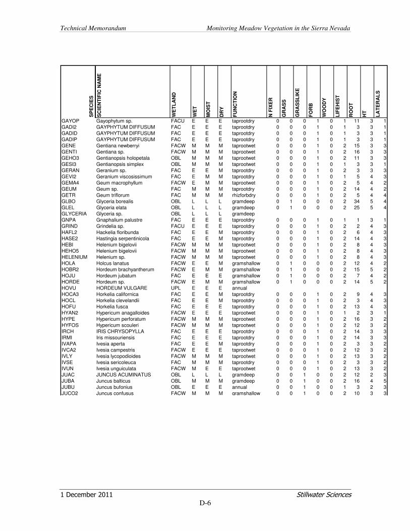
Technical Memorandum Monitoring Meadow Vegetation in the Sierra Nevada
1 December 2011 Stillwater Sciences
D-6
SP
EC
IES
SC
IEN
TIF
IC N
AM
E
WE
TL
AN
D
WE
T
MO
IST
DR
Y
FU
NC
TIO
N
N F
IXE
R
GR
AS
S
GR
AS
SL
IKE
FO
RB
WO
OD
Y
LIF
EH
IST
RO
OT
HT
LA
TE
RA
LS
GAYOP Gayophytum sp. FACU E E E taprootdry 0 0 0 1 0 1 11 3 1
GADI2 GAYPHYTUM DIFFUSUM FAC E E E taprootdry 0 0 0 1 0 1 3 3 1
GADID GAYPHYTUM DIFFUSUM FAC E E E taprootdry 0 0 0 1 0 1 3 3 1
GADIP GAYPHYTUM DIFFUSUM FAC E E E taprootdry 0 0 0 1 0 1 3 3 1
GENE Gentiana newberryi FACW M M M taprootwet 0 0 0 1 0 2 15 3 3
GENTI Gentiana sp. FACW M M M taprootwet 0 0 0 1 0 2 16 3 3
GEHO3 Gentianopsis holopetala OBL M M M taprootwet 0 0 0 1 0 2 11 3 3
GESI3 Gentianopsis simplex OBL M M M taprootwet 0 0 0 1 0 1 3 3 1
GERAN Geranium sp. FAC E E M taprootdry 0 0 0 1 0 2 3 3 3
GEVI2 Geranium viscosissimum FAC E M M taprootdry 0 0 0 1 0 1 5 4 3
GEMA4 Geum macrophyllum FACW E M M taprootwet 0 0 0 1 0 2 5 4 2
GEUM Geum sp. FAC M M M taprootdry 0 0 0 1 0 2 14 4 2
GETR Geum triflorum FAC M M M rhizforbdry 0 0 0 1 0 2 5 4 4
GLBO Glyceria borealis OBL L L L gramdeep 0 1 0 0 0 2 34 5 4
GLEL Glyceria elata OBL L L L gramdeep 0 1 0 0 0 2 25 5 4
GLYCERIA Glyceria sp. OBL L L L gramdeep
GNPA Gnaphalium palustre FAC E E E taprootdry 0 0 0 1 0 1 1 3 1
GRIND Grindelia sp. FACU E E E taprootdry 0 0 0 1 0 2 2 4 3
HAFL2 Hackelia floribunda FAC E E M taprootdry 0 0 0 1 0 2 6 4 3
HASE2 Hastingia serpentinicola FAC E E M taprootdry 0 0 0 1 0 2 14 4 3
HEBI Helenium bigelovii FACW M M M taprootwet 0 0 0 1 0 2 8 4 3
HEHO5 Helenium bigelovii FACW M M M taprootwet 0 0 0 1 0 2 8 4 3
HELENIUM Helenium sp. FACW M M M taprootwet 0 0 0 1 0 2 8 4 3
HOLA Holcus lanatus FACW E E M gramshallow 0 1 0 0 0 2 12 4 2
HOBR2 Hordeum brachyantherum FACW E M M gramshallow 0 1 0 0 0 2 15 5 2
HOJU Hordeum jubatum FAC E E E gramshallow 0 1 0 0 0 2 7 4 2
HORDE Hordeum sp. FACW E M M gramshallow 0 1 0 0 0 2 14 5 2
HOVU HORDEUM VULGARE UPL E E E annual
HOCA3 Horkelia californica FAC E E M taprootdry 0 0 0 1 0 2 9 4 3
HOCL Horkelia clevelandii FAC E E M taprootdry 0 0 0 1 0 2 3 4 3
HOFU Horkelia fusca FAC E E E taprootdry 0 0 0 1 0 2 13 4 3
HYAN2 Hypericum anagalloides FACW E E E taprootwet 0 0 0 1 0 1 2 3 1
HYPE Hypericum perforatum FACW M M M taprootwet 0 0 0 1 0 2 16 3 2
HYFOS Hypericum scouleri FACW M M M taprootwet 0 0 0 1 0 2 12 3 2
IRCH IRIS CHRYSOPYLLA FAC E E E taprootdry 0 0 0 1 0 2 14 3 3
IRMI Iris missouriensis FAC E E E taprootdry 0 0 0 1 0 2 14 3 3
IVAPA Ivesia aperta FAC E E M taprootdry 0 0 0 1 0 2 3 3 2
IVCA2 Ivesia campestris FACW E E E taprootwet 0 0 0 1 0 2 12 3 2
IVLY Ivesia lycopodioides FACW M M M taprootwet 0 0 0 1 0 2 13 3 2
IVSE Ivesia sericoleuca FAC M M M taprootdry 0 0 0 1 0 2 3 3 2
IVUN Ivesia unguiculata FACW M E E taprootwet 0 0 0 1 0 2 13 3 2
JUAC JUNCUS ACUMINATUS OBL L L L gramdeep 0 0 1 0 0 2 12 2 3
JUBA Juncus balticus OBL M M M gramdeep 0 0 1 0 0 2 16 4 5
JUBU Juncus bufonius OBL E E E annual 0 0 1 0 0 1 3 2 3
JUCO2 Juncus confusus FACW M M M gramshallow 0 0 1 0 0 2 10 3 3

Technical Memorandum Monitoring Meadow Vegetation in the Sierra Nevada
1 December 2011 Stillwater Sciences
D-7
SP
EC
IES
SC
IEN
TIF
IC N
AM
E
WE
TL
AN
D
WE
T
MO
IST
DR
Y
FU
NC
TIO
N
N F
IXE
R
GR
AS
S
GR
AS
SL
IKE
FO
RB
WO
OD
Y
LIF
EH
IST
RO
OT
HT
LA
TE
RA
LS
JUEN2 Juncus ensifolius OBL L L L gramdeep 0 0 1 0 0 2 27 4 5
JULO Juncus longistylis FACW L L L gramshallow 0 0 1 0 0 2 8 4 4
JUME3 Juncus mertensianus OBL L L L gramshallow 0 0 1 0 0 2 6 3 4
JUME Juncus mexicanus FACW M M M gramdeep 0 0 1 0 0 2 18 4 4
JUME4 Juncus mexicanus FACW M M M gramdeep 0 0 1 0 0 2 18 4 4
JUNE Juncus nevadensis FACW L L L gramdeep 0 0 1 0 0 2 22 4 4
JUOR Juncus orthophyllus FACW M M L gramdeep 0 0 1 0 0 2 17 4 3
JUOX Juncus oxymeris FACW L L L gramdeep 0 0 1 0 0 2 19 4 3
JUPA Juncus parryi FACU E E M gramdry 0 0 1 0 0 2 4 4 3
JUPA2 Juncus patens FACW M M L gramshallow 0 0 1 0 0 2 11 4 3
JUPH Juncus phaeocephalus FACW L L L gramdeep 0 0 1 0 0 2 15 4 5
JUNCU JUNCUS SP. FACW L L L gramdeep 0 0 1 0 0 2 15 3 4
JUNCUS JUNCUS SP. FACW L L L gramdeep 0 0 1 0 0 2 15 3 4
JUTE JUNUS TENUIS FACW M M M gramshallow 0 0 1 0 0 2 2 1
KAPO KALMIA POLIFOLIA FACW L L L rhizforbwet 0 0 0 1 1 2 17 3 4
KAPOM3 KALMIA POLIFOLIA FACW L L L rhizforbwet 0 0 0 1 1 2 17 3 4
LASE Lactuca serriola FACU E E E taprootdry 0 0 0 1 0 1 2 3 1
LEPID Lepidium sp. FACU E E E taprootdry 0 0 0 1 0 1 10 3 1
LESSI LESSINGIA SP. FAC E E M
LENE5 Lewisia nevadensis FACU L L L taprootdry 0 0 0 1 0 2 7 3 3
ELTR3 Leymus triticoides FAC M M L gramshallow 0 1 0 0 0 2 8 5 5
LETR5 LEYMUS TRITICOIDES FAC M M L gramshallow 0 1 0 0 0 2 14 5 2
LIHA Linanthus harknessii FACU E E E taprootdry 0 0 0 1 0 1 4 2 1
LICI Linathus ciliatus FACU E E E taprootdry 0 0 0 1 0 1 5 2 1
LINAN Linathus sp. FACU E E E taprootdry 0 0 0 1 0 1 2 3 1
LILE3 Linum lewisii FACU E E E taprootdry 0 0 0 1 0 2 12 3 3
LOMU LOLIUM PERENNE UPL E E E annual
LOMAT Lomatium sp. FACU E E E taprootdry 0 0 0 1 0 2 1 3 3
LOCO6 Lotus corniculatus FAC E E M taprootdry 0 0 0 1 0 2 7 3 2
LOOB Lotus oblongifolius FACW E E M taprootwet 0 0 0 1 0 2 3 3 2
LOOB2 Lotus oblongifolius FACW E E M taprootwet 0 0 0 1 0 2 3 3 2
LOPI2 Lotus pinnatus FACW E E M taprootwet 0 0 0 1 0 2 4 3 2
LOPU3 Lotus purshianus FAC E E E taprootdry 0 0 0 1 0 1 10 3 1
LOTUS Lotus sp. FAC E E E taprootdry 0 0 0 1 0 1 13 3 1
LOST4 Lotus strigosus FAC E E E taprootdry 0 0 0 1 0 1 1 3 1
LUAR3 Lupinus argenteus FACU E E E taprootdry 0 0 0 1 0 2 6 3 3
LUBI Lupinus bicolor FACU E E E taprootdry 0 0 0 1 0 1 3 3 1
LUCA LUPINUS CAUDATUS UPL E E E taprootdry 0 0 0 1 0 2 2 2 3
LULES2 Lupinus lepidus var. sellulus UPL E E M taprootdry 0 0 0 1 0 2 4 1 3
LUPO2 Lupinus polyphyllus FACW M M M taprootwet 0 0 0 1 0 2 4 5 3
LUPIN Lupinus sp. FACU E E E taprootdry 0 0 0 1 0 2 9 3 3
LUCO6 Luzula comosa FACW L L L gramshallow 0 0 1 0 0 2 10 4 4
LUOR4 Luzula orestera OBL L L L gramshallow 0 0 1 0 0 2 7 4 4
LUPA4 Luzula parviflora FAC E E M gramshallow 0 0 1 0 0 2 15 4 4
LUZUL Luzula sp. FAC L L L gramshallow 0 0 1 0 0 2 16 4 4

Technical Memorandum Monitoring Meadow Vegetation in the Sierra Nevada
1 December 2011 Stillwater Sciences
D-8
SP
EC
IES
SC
IEN
TIF
IC N
AM
E
WE
TL
AN
D
WE
T
MO
IST
DR
Y
FU
NC
TIO
N
N F
IXE
R
GR
AS
S
GR
AS
SL
IKE
FO
RB
WO
OD
Y
LIF
EH
IST
RO
OT
HT
LA
TE
RA
LS
MELU Medicago lupulina FAC E E E taprootdry 0 0 0 1 0 1 2 3 2
MEDIC Medicago sp. FAC E E E taprootdry 0 0 0 1 0 1 3 3 1
MEBU Melica bulbosa UPL E E E gramupl 0 1 0 0 0 2 14 4 3
MEAR4 Mentha arvensis FACW E E taprootwet 0 0 0 1 0 2 7 3 2
MECI3 Mertensia ciliata FACW M M M rhizforbwet 0 0 0 1 0 2 3 3 4
MIGU Mimulus guttatus OBL M M M rhizforbwet 0 0 0 1 0 2 12 3 4
MIMO3 Mimulus moschatus OBL M M M taprootwet 0 0 0 1 0 2 5 3 2
MIPR Mimulus primuloides OBL M M M rhizforbwet 0 0 0 1 0 2 19 3 4
MIPRL Mimulus primuloides OBL M M M rhizforbwet 0 0 0 1 0 2 19 3 4
MOOD Monardella odoratissima FACW M M M taprootwet 0 0 0 1 0 2 8 3 2
MOCH Montia chamissoi OBL M M M rhizforbwet 0 0 0 1 0 2 15 3 4
MOLI4 Montia linearis OBL E E E taprootwet 0 0 0 1 0 1 14 3 1
MUAS Muhlenbergia asperifolia FACW M E M gramshallow 0 1 0 0 0 2 18 4 4
MUFI Muhlenbergia filiformis OBL M M M annual 0 1 0 0 0 1 18 3 1
MUFI2 Muhlenbergia filiformis OBL M M M annual 0 1 0 0 0 1 18 3 1
MURI Muhlenbergia richardsonis FAC E M M gramshallow 0 1 0 0 0 2 14 3 4
MURI2 Muhlenbergia rigens FAC E M L gamshallow 0 1 0 0 0 2 10 5 3
NABR Navarretia breweri FACU E E E taprootdry 0 0 0 1 0 1 2 3 1
NAIN2 Navarretia intertexta FACU E E E taprootdry 0 0 0 1 0 1 7 3 1
NALE Navarretia leucocephala OBL E E E taprootwet 0 0 0 1 0 1 10 3 1
NAVAR Navarretia sp. FACU E E E taprootdry 0 0 0 1 0 1 17 3 1
NEPE Nemophila pedunculata FAC E E E taprootdry 0 0 0 1 0 1 14 3 1
NEMOP Nemophila sp. FACW E E E taprootwet 0 0 0 1 0 1 11 3 1
ORLU2 Orthocarpus luteus FACU E E E taprootdry 0 0 0 1 0 1 0 3 2
ORTHO Orthocarpus sp. FAC E E E taprootdry 0 0 0 1 0 1 13 3 1
OXOC Oxypolis occidentalis FACW L L L taprootwet 0 0 0 1 0 2 15 3 2
PANIC Panicum sp. FAC M M M taprootdry 0 0 0 1 0 2 14 3 2
PEAT Pedicularis attollens OBL L L L taprootwet 0 0 0 1 0 2 15 4 3
PEGR2 Pedicularis groenlandica OBL L L L taprootwet 0 0 0 1 0 2 8 4 2
PEDIC Pedicularis sp. FACW L L L taprootwet 0 0 0 1 0 2 12 4 3
PEHE2 Penstemon herterodoxus FAC E E M taprootdry 0 0 0 1 0 2 22 3 2
PELA7 Penstemon laetus FAC E E M taprootdry 0 0 0 1 0 2 10 3 2
PEPR2 Penstemon procerus FAC E E M taprootdry 0 0 0 1 0 2 7 3 2
PERY Penstemon rydbergii FAC M M M taprootdry 0 0 0 1 0 2 16 3 2
PERYO Penstemon rydbergii FAC M M M taprootdry 0 0 0 1 0 2 10 3 2
PENST Penstemon sp. FAC M M M taprootdry 0 0 0 1 0 2 25 3 2
PERID Perderidia sp. FAC M M M taprootdry 0 0 0 1 0 2 14 4 2
PELE5 Perideridia lemmonii FAC E E M taprootdry 0 0 0 1 0 2 26 4 2
PEPA21 Perideridia parishii FACW E E M taprootwet 0 0 0 1 0 2 15 4 2
PEPAL Perideridia parishii UPL E E M taprootdry 0 0 0 1 0 2 10 2 2
PHBO Phalacroseris bolanderi FACW M M M taprootwet 0 0 0 1 0 2 16 3 3
PHBO2 Phalacroseris bolanderi FACW M M M taprootwet 0 0 0 1 0 2 16 3 3
PHAQ Phalaris aquatica FACW E E E gramshallow 0 1 0 0 0 2 15 5 4
PHAL2 Phleum alpinum FACW L L L gramshallow 0 1 0 0 0 2 20 4 3
PHPR3 Phleum pratense FAC E E M gramshallow 0 1 0 0 0 2 18 5 3
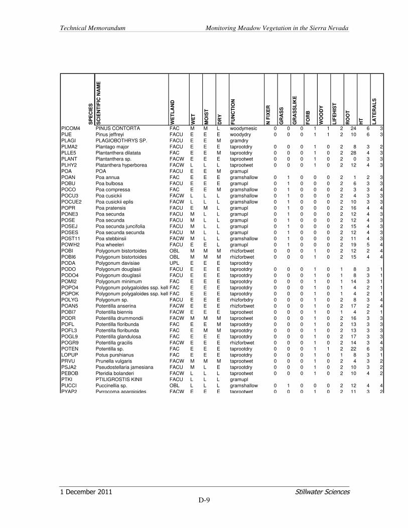
Technical Memorandum Monitoring Meadow Vegetation in the Sierra Nevada
1 December 2011 Stillwater Sciences
D-9
SP
EC
IES
SC
IEN
TIF
IC N
AM
E
WE
TL
AN
D
WE
T
MO
IST
DR
Y
FU
NC
TIO
N
N F
IXE
R
GR
AS
S
GR
AS
SL
IKE
FO
RB
WO
OD
Y
LIF
EH
IST
RO
OT
HT
LA
TE
RA
LS
PICOM4 PINUS CONTORTA FAC M M L woodymesic 0 0 0 1 1 2 24 6 3
PIJE Pinus jeffreyi FACU E E E woodydry 0 0 0 1 1 2 10 6 3
PLAGI PLAGIOBOTHRYS SP. FACU E E M gramdry
PLMA2 Plantago major FACU E E E taprootdry 0 0 0 1 0 2 8 3 2
PLLE5 Plantanthera dilatata FAC E E M taprootdry 0 0 0 1 0 2 28 4 3
PLANT Plantanthera sp. FACW E E E taprootwet 0 0 0 1 0 2 0 3 3
PLHY2 Platanthera hyperborea FACW L L L taprootwet 0 0 0 1 0 2 12 4 3
POA POA FACU E E M gramupl
POAN Poa annua FAC E E E gramshallow 0 1 0 0 0 2 1 2 3
POBU Poa bulbosa FACU E E E gramupl 0 1 0 0 0 2 6 3 3
POCO Poa compressa FAC E E M gramshallow 0 1 0 0 0 2 3 3 4
POCU3 Poa cusickii FACW L L L gramshallow 0 1 0 0 0 2 4 3 3
POCUE2 Poa cusickii eplis FACW L L L gramshallow 0 1 0 0 0 2 10 3 3
POPR Poa pratensis FACU E M L gramupl 0 1 0 0 0 2 16 4 4
PONE3 Poa secunda FACU M L L gramupl 0 1 0 0 0 2 12 4 3
POSE Poa secunda FACU M L L gramupl 0 1 0 0 0 2 12 4 3
POSEJ Poa secunda juncifolia FACU M L L gramupl 0 1 0 0 0 2 15 4 3
POSES Poa secunda secunda FACU M L L gramupl 0 1 0 0 0 2 12 4 3
POST11 Poa stebbinsii FACW M L L gramshallow 0 1 0 0 0 2 11 4 3
POWH2 Poa wheeleri FACU E E L gramupl 0 1 0 0 0 2 19 5 4
POBI Polygonum bistortoides OBL M M M rhizforbwet 0 0 0 1 0 2 12 2 4
POBI6 Polygonum bistortoides OBL M M M rhizforbwet 0 0 0 1 0 2 15 4 4
PODA Polygonum davisiae UPL E E E taprootdry
PODO Polygonum douglasii FACU E E E taprootdry 0 0 0 1 0 1 8 3 1
PODO4 Polygonum douglasii FACU E E E taprootdry 0 0 0 1 0 1 8 3 1
POMI2 Polygonum minimum FAC E E E taprootdry 0 0 0 1 0 1 14 3 1
POPO4 Polygonum polygaloides ssp. kelloFAC E E E taprootdry 0 0 0 1 0 1 4 2 1
POPOK Polygonum polygaloides ssp. kelloFAC E E E taprootdry 0 0 0 1 0 1 4 2 1
POLYG Polygonum sp. FACU E E E rhizforbdry 0 0 0 1 0 2 8 3 4
POAN5 Potentilla anserina FACW E E E rhizforbwet 0 0 0 1 0 2 17 2 4
POBI7 Potentilla biennis FACW E E E taprootwet 0 0 0 1 0 1 4 2 1
PODR Potentilla drummondii FACW M M M taprootwet 0 0 0 1 0 2 16 3 3
POFL Potentilla floribunda FAC E E M taprootdry 0 0 0 1 0 2 13 3 3
POFL3 Potentilla floribunda FAC E M M taprootdry 0 0 0 1 0 2 13 3 3
POGL9 Potentilla glandulosa FAC E E E taprootdry 0 0 0 1 0 2 17 3 3
POGR9 Potentilla gracilis FACW E E E rhizforbwet 0 0 0 1 0 2 14 3 4
POTEN Potentilla sp. FAC E E E taprootdry 0 0 0 1 1 2 22 6 3
LOPUP Potus purshianus FAC E E E taprootdry 0 0 0 1 0 1 8 3 1
PRVU Prunella vulgaris FACW M M M taprootwet 0 0 0 1 0 2 4 3 2
PSJA2 Pseudostellaria jamesiana FACU M L E taprootdry 0 0 0 1 0 2 10 3 2
PEBOB Pteridia bolanderi FACW L L L taprootwet 0 0 0 1 0 2 10 4 2
PTKI PTILIGROSTIS KINII FACU L L L gramupl
PUCCI Puccinellia sp. OBL L L L gramshallow 0 1 0 0 0 2 12 4 4
PYAP2 Pyrrocoma apargioides FACW E E E taprootwet 0 0 0 1 0 2 11 3 2

Technical Memorandum Monitoring Meadow Vegetation in the Sierra Nevada
1 December 2011 Stillwater Sciences
D-10
SP
EC
IES
SC
IEN
TIF
IC N
AM
E
WE
TL
AN
D
WE
T
MO
IST
DR
Y
FU
NC
TIO
N
N F
IXE
R
GR
AS
S
GR
AS
SL
IKE
FO
RB
WO
OD
Y
LIF
EH
IST
RO
OT
HT
LA
TE
RA
LS
RAOC Ranunculus occidentalis FACW E E E taprootwet 0 0 0 1 0 2 11 3 2
RAOR3 Ranunculus orthorhynchus FACW E E E taprootwet 0 0 0 1 0 2 16 3 2
RANUN Ranunculus sp. FACW E E M taprootwet 0 0 0 1 0 2 20 3 2
RIAU Ribes aureum FACW L L L rhizforbwet 0 0 0 1 1 2 3 6 4
RICE Ribes cereum FACU E E E taprootdry 0 0 0 1 1 2 1 6 3
RIIN2 Ribes inerme FACW L L L taprootwet 0 0 0 1 1 2 2 6 3
RIMO2 Ribes montigenum FACW L L L taprootwet 0 0 0 1 1 2 2 6 3
ROCU Rorippa curvisiliqua OBL E E E taprootwet 0 0 0 1 0 1 1 3 1
RONA2 Rorippa nasturtium-aquaticum OBL E E E taprootwet 0 0 0 1 0 2 13 3 2
RORIPPA Rorippa sp. OBL M M M taprootwet 0 0 0 1 0 2 13 3 2
ROWOU Rosa woodsii FAC M L L woodymesic 0 0 0 1 1 2 2 6 4
RUFU5 RUBUS WHEELERI UPL E E E woodydry
RUDBE Rudbeckia sp. FACU E E E rhizforbdry 0 0 0 1 0 2 4 3 4
RUAC3 Rumex acetosella FACW E E M taprootwet 0 0 0 1 0 2 12 3 3
RUCR Rumex crispus FACW E E E taprootwet 0 0 0 1 0 2 12 3 3
RUPA6 Rumex paucifolius OBL E E E taprootwet 0 0 0 1 0 2 7 3 3
RUMEX Rumex sp. FACW E E E taprootwet 0 0 0 1 0 2 3 3 3
SASA Sagina saginoides FACW E E E taprootwet 0 0 0 1 0 2 0 2 2
SAGE2 Salix geyeriana FACW L L L woodywet 0 0 0 1 1 2 10 6 3
SALE Salix lemmonii FACW L L L woodywet 0 0 0 1 1 2 15 6 3
SAOR Salix orestera FACW L L L woodywet 0 0 0 1 1 2 15 6 3
SAPL Salix planifolia FACW L L L wodywet 0 0 0 1 1 2 2 6 3
SAOR2 Saxifraga oregana OBL M M M taprootwet 0 0 0 1 0 2 12 4 2
SAXIF Saxifraga sp. FACW M M M taprootwet 0 0 0 1 0 2 12 3 2
SCCL Scirpus clemantis FACW L L L gramshallow 0 0 1 0 0 2 10 2 4
SCCO Scirpus congdonii OBL L L L gramdeep 0 0 1 0 0 2 22 4 4
SCMI Scirpus microcarpus OBL L L L gramdeep 0 0 1 0 0 2 20 4 5
SCMI2 Scirpus microcarpus OBL L L L gramdeep 0 0 1 0 0 2 20 4 5
SCIRP Scirpus sp. OBL L L L gramdeep 0 0 1 0 0 2 15 4 5
SCIRPUS Scirpus SP. OBL L L L gramdeep 0 0 1 0 0 2 20 4 5
SESES Senecia serra OBL M E M taprootwet 0 0 0 1 0 2 12 5 2
SEHY2 Senecio hydrophilus OBL M M M taprootwet 0 0 0 1 0 2 14 5 2
SECA2 Senecio serra FACW M M M taprootwet 0 0 0 1 0 2 2 4 2
SETR Senecio triangularis FACW M M M rhizforbwet 0 0 0 1 0 2 18 5 4
SIPR Sibbaldia procumbens FAC E L L taprootdry 0 0 0 1 0 2 11 2 2
SIMA2 Sidalcea malviflora FAC E E M taprootdry 0 0 0 1 0 2 5 3 2
SIOR Sidalcea oregana OBL E E E taprootwet 0 0 0 1 0 2 5 4 2
SIRA Sidalcea ranunculacea OBL E E E taprootwet 0 0 0 1 0 2 3 4 2
SIRE Sidalcea reptans OBL E E E taprootwet 0 0 0 1 0 2 15 4 2
SIDAL Sidalcea sp. FACW E E E taprootwet 0 0 0 1 0 2 5 3 2
SILEN Silene sp. FAC E E M taprootdry 0 0 0 1 0 2 22 4 2
SISYM Sisymbrium sp. FACW M M M taprootwet 0 0 0 1 0 2 1 4 2
SIID Sisyrinchium idahoense FACW M M M taprootwet 0 0 0 1 0 2 10 4 2
SISYR Sisyrinchium sp. FAC E E M taprootdry 0 0 0 1 0 2 15 4 2
SOCA5 Solidaga canadensis FAC E E M taprootdry 0 0 0 1 0 2 10 4 3

Technical Memorandum Monitoring Meadow Vegetation in the Sierra Nevada
1 December 2011 Stillwater Sciences
D-11
SP
EC
IES
SC
IEN
TIF
IC N
AM
E
WE
TL
AN
D
WE
T
MO
IST
DR
Y
FU
NC
TIO
N
N F
IXE
R
GR
AS
S
GR
AS
SL
IKE
FO
RB
WO
OD
Y
LIF
EH
IST
RO
OT
HT
LA
TE
RA
LS
SPRU Spergularia rubra FAC E E E taprootdry 0 0 0 1 0 1 10 3 1
SPCA5 Sphenosciadium capitellatum OBL L L L taprootwet 0 0 0 1 0 2 12 4 2
SPRO Spiranthes romanzoffiana OBL L L L taprootwet 0 0 0 1 0 2 21 4 2
STBU Stachys bullata FAC E E M taprootdry 0 0 0 1 0 2 27 4 2
STAJR Stachys rigida FAC E E M taprootdry 0 0 0 1 0 2 10 4 2
STLO Stellaria longipes FACW M M M rhizforbwet 0 0 0 1 0 2 17 4 4
STLO2 Stellaria longipes FACW M M M rhizforbwet 0 0 0 1 0 2 17 4 4
STLOL5 Stellaria longipes FACW M M M rhizforbwet 0 0 0 1 0 2 17 4 4
STELL Stellaria sp. FACW M M M rhizforbwet 0 0 0 1 0 2 27 4 4
ASAD6 Symphyotrichum ascendens FAC E E E rhizforbdry 0 0 0 1 0 2 12 4 4
TACA8 TAENIATHERUM CAPUT-MEDUSUPL E E E annual
TAOF Taraxacum officinale FACW E E E taprootwet 0 0 0 1 0 2 4 3 2
TARAX Taraxacum sp. FACW E E E taprootwet 0 0 0 1 0 2 4 3 2
THFE THALICTRUM FENDERLIANAFACU E E E taprootdry 0 0 0 1 0 2 2 3 3
TOGLO2 TOFIELDIA OBL L L L taprootwet
TRAL5 Triantha occidentalis FAC E E E taprootdry 0 0 0 1 0 1 1 3 1
TROB Trichostema oblongum FACW E E E Nfix 0 0 1 0 1 2 4 1
TRHI4 Tridolium hirtum FACU E E E taprootdry 1 0 0 1 0 1 2 3 2
TRBO Trifolium bolanderi OBL M M M Nfix 1 0 0 1 0 1 3 1 1
TRBO3 Trifolium bolanderi OBL E E E Nfix 1 0 0 1 0 1 12 3 2
TRCY Trifolium cyathiferum FACW E E E Nfix 1 0 0 1 0 1 2 3 1
TRER2 TRIFOLIUM ERIOCEPHALUM FAC M M M Nfix
TRLE2 Trifolium lemmonii FACW M M M Nfix 1 0 0 1 0 2 6 3 2
TRLO Trifolium longipes FACW M M M Nfix 1 0 0 1 0 2 12 3 4
TRMI4 Trifolium microcephalum FACW E E E Nfix 1 0 0 1 0 1 9 3 1
TRMI5 TRIFOLIUM MOICRODON UPL E E E Nfix
TRMO Trifolium monanthum FACW M M M Nfix 1 0 0 1 0 2 12 3 2
TRMO2 Trifolium monanthum FACW M M M Nfix 1 0 0 1 0 2 12 3 2
TRRE Trifolium repens FAC E E E Nfix 1 0 0 1 0 2 3 3 4
TRRE3 Trifolium repens FAC E E E Nfix 1 0 0 1 0 2 3 3 4
TRIFO Trifolium TRIFOLIUM FACW M M M Nfix 1 0 0 1 0 2 2 5 2
TRVA Trifolium variegatum FACW M M M taprootwet 1 0 0 1 0 1 8 3 1
TRWI3 Trifolium wildenovii FACW E E E taprootwet 1 0 0 1 0 1 1 3 1
TRWO Trifolium wormskioldii OBL M M M Nfix 1 0 0 1 0 2 16 3 4
TRSP2 Trisetum spicatum FACW L L L gramshallow 0 1 0 0 0 2 11 4 3
TRWO3 Trisetum wolfii FACW L L L gramshallow 0 1 0 0 0 2 12 4 3
TRHY3 Triteleia hyacinthina FACW E M M taprootwet 1 0 0 1 0 2 10 3 3
2GRAM UNK graminoid FAC E M L gramupl
URDI Urtica dioica FACW E E E taprootwet 0 0 0 1 0 2 2 4 1
URTIC Urtica sp. FACW E E E rhizforbwet 0 0 0 1 0 2 13 4 4
VACA VACCINIUM CESPITOSUM FACW L L L taprootwet 0 0 0 1 1 2 12 5 3
VACE VACCINIUM CESPITOSUM FACW L L L taprootwet 0 0 0 1 1 2 12 5 3
VACCI VACCINIUM SP. FACW L L L taprootwet 0 0 0 1 1 2 12 5 3
VAUL VACCINIUM ULIGINOSUM FACW L L L taprootwet 0 0 0 1 1 2 12 5 3
VAULO VACCINIUM ULIGINOSUM FACW L L L taprootwet 0 0 0 1 1 2 12 5 3

Technical Memorandum Monitoring Meadow Vegetation in the Sierra Nevada
1 December 2011 Stillwater Sciences
D-12
SP
EC
IES
SC
IEN
TIF
IC N
AM
E
WE
TL
AN
D
WE
T
MO
IST
DR
Y
FU
NC
TIO
N
N F
IXE
R
GR
AS
S
GR
AS
SL
IKE
FO
RB
WO
OD
Y
LIF
EH
IST
RO
OT
HT
LA
TE
RA
LS
VELA Verbena lasiostachys FAC E E E taprootdry 0 0 0 1 0 2 16 4 2
VEAM2 Veronica americana OBL M M M rhizforbwet 0 0 0 1 0 2 20 3 4
VEAR Veronica arvensis* FAC E E M taprootdry 0 0 0 1 0 1 7 1 3
VECH VERONICA CHAMAEDRYS UPL E E E taprootdry
VESC2 Veronica scutellata OBL M M M taprootwet 0 0 0 1 0 2 17 3 2
VERON Veronica sp. FAC M M M taprootdry 0 0 0 1 0 1 14 3 2
VEWO2 Veronica wormskjoldii FACW M M M rhizforbwet 0 0 0 1 0 2 4 1 4
VIAM Vicia americana FAC E E M rhizforbdry 0 0 0 1 0 2 6 4 4
VICIA Vicia sp. FAC E E E taprootdry 0 0 0 1 0 2 2 3 2
VIAD Viola adunca FAC M M M taprootdry 0 0 0 1 0 2 5 3 2
VIGL Viola glabella FACW M M M taprootwet 0 0 0 1 0 2 22 3 2
VIMA Viola macloskeyi OBL M M M taprootwet 0 0 0 1 0 2 17 3 2
VIMA2 Viola macloskeyi OBL M M M taprootwet 0 0 0 1 0 2 17 3 2
VIOLA Viola sp. FACW M M M taprootwet 0 0 0 1 0 2 21 3 2
VUMY VUPLIA MYUROS UPL E E E annual 0 0 0 1 0 1 1 1 1
VUOC VUPLIA OCTOFLORA UPL E E E annual 0 0 0 1 0 1 1 1 1
VULPIA VUPLIA SP. UPL E E E annual 0 0 0 1 0 1 1 1 1
WYOV Wyethia ovina FACU E E E taprootdry 0 0 0 1 0 2 2 3 2
WYETH Wyethis ap. FACU E E E taprootdry 0 0 0 1 0 2 2 4 3
DODEC FACW M M M taprootwet 0 0 0 1 0 2 11 4 3