monitoring post-fire vegetation rehabilitation projects: a common

Monitoring Post-Fire Vegetation Rehabilitation Projects: A Common Approach for Non-Forested Ecosystems

U.S. Department of the InteriorU.S. Geological Survey

Scientific Investigations Report 2006-5048

Cover: Fire on front and back cover and upper-left quadrant of circle: Farewell Bend Fire, 2005; photo by Brian Watts. Seeding operation in lower-left quadrant of circle; photo by Scott Shaff.


By Troy A. Wirth and David A. Pyke

Scientific Investigations Report 2006-5048

U.S. Department of the InteriorU.S. Geological Survey

U.S. Department of the InteriorDIRK KEMPTHORNE, Secretary

U.S. Geological SurveyMark D. Meyers, Director

U.S. Geological Survey, Reston, Virginia: 2007

For product and ordering information: World Wide Web: http://www.usgs.gov/pubprod Telephone: 1-888-ASK-USGS

For more information on the USGS--the Federal source for science about the Earth, its natural and living resources, natural hazards, and the environment: World Wide Web: http://www.usgs.gov Telephone: 1-888-ASK-USGS

Any use of trade, product, or firm names is for descriptive purposes only and does not imply endorsement by the U.S. Government.

Although this report is in the public domain, permission must be secured from the individual copyright owners to reproduce any copyrighted materials contained within this report.

Suggested citation:Wirth, Troy A., and Pyke, David A., 2007, Monitoring post-fire vegetation rehabilitation projects—A common approach for non-forested ecosystems: U.S. Geological Survey Scientific Investigations Report 2006-5048, 36 p.

http://www.usgs.gov/pubprod

http://www.usgs.gov

iii

Contents

Abstract ...........................................................................................................................................................1Introduction.....................................................................................................................................................1 Current Monitoring Methods Used by Field Personnel ...........................................................................2

Bureau of Land Management .............................................................................................................2USDA Forest Service (USFS) ..............................................................................................................3National Park Service (NPS) ...............................................................................................................5U.S. Fish and Wildlife Service (USFWS) ...........................................................................................5Bureau of Indian Affairs (BIA) ............................................................................................................5

Monitoring Publications................................................................................................................................6Measuring and Monitoring Plant Populations (Elzinga et al., 1998) .............................................7

Monitoring Program Design .......................................................................................................8Sampling Approach .....................................................................................................................8

Sampling Vegetation Attributes (Interagency Technical Reference, 1999) ................................9Monitoring Program Design .......................................................................................................9Sampling Approach .....................................................................................................................9

Fire Monitoring Handbook (USDI National Park Service, 2003) ....................................................9Monitoring Program Design .......................................................................................................9Sampling Approach ...................................................................................................................10

Monitoring Manual for Grassland, Shrubland, and Savanna Ecosystems (Herrick et al. 2005a, 2005b) .........................................................................................................................10

Monitoring Program Design .....................................................................................................10Sampling Approach ...................................................................................................................11

Fire Effects Monitoring and Inventory Protocol (Lutes et al., 2006) ..........................................12Monitoring Program Design .....................................................................................................12Sampling Approach ...................................................................................................................12

Fuel and Fire Effects Monitoring Guide (USDI Fish and Wildlife Service, 1999) ......................12Monitoring Program Design .....................................................................................................13Sampling Approach ...................................................................................................................13

Range and Training Land Assessment Technical Reference Manual (U.S. Army, 2006) .......13Monitoring Program Design .....................................................................................................13Sampling Approach ...................................................................................................................13

National Assessment Programs ................................................................................................................13National Resources Inventory (NRI) ................................................................................................14Forest Inventory and Analysis (FIA) (USDA Forest Service, 2003b) ...........................................14

Common Elements of Monitoring Program Designs ..............................................................................14Objectives.............................................................................................................................................14Stratification ........................................................................................................................................15Controls.................................................................................................................................................15Random Sampling ...............................................................................................................................16Data Quality..........................................................................................................................................16Statistical Analysis .............................................................................................................................17

iv

Contents—continuedField Techniques .................................................................................................................................17

Cover .........................................................................................................................................18Density .........................................................................................................................................18Gap Intercept ..............................................................................................................................19Non-Standard Techniques .......................................................................................................19Erosion Monitoring ....................................................................................................................19

A Common Approach for Monitoring Future ES&R Treatments ...........................................................20Conclusions...................................................................................................................................................21Acknowledgements .....................................................................................................................................22References ....................................................................................................................................................22Appendixes ...................................................................................................................................................24

Appendix A-1. Advantages and disadvantages of measuring the three basic vegetation attributes .............................................................................................................24

Appendix A-2. Advantages and disadvantages of three different methods of estimating cover ....................................................................................................................25

Appendix B - Example Project Using the Six Common Elements .......................................................26

Figures Figure 1. Percent proposed monitoring techniques on ES&R projects on BLM lands

in the northern intermountain west of Idaho, Nevada, Oregon, and Utah during four three-year periods from 1988 to 1999 ...................................................................4

Figure 2. Similarities between monitoring and research. Bold text indicates elements in common ........................................................................................................................................21

Tables Table 1. Quantitative vegetation monitoring methods that were used during 2004 by

BLM offices ....................................................................................................................................3 Table 2. Citations and websites for the seven vegetation monitoring manuals reviewed

in this publication ..........................................................................................................................6 Table 3. Monitoring elements and methods discussed in the seven monitoring manuals .............7

v

Conversion FactorsEnglish to Metric

Multiply By To obtainLength

inch (in.) 2.54 centimeter (cm)inch (in.) 25.4 millimeter (mm)foot (ft) 0.3048 meter (m)mile (mi) 1.609 kilometer (km)mile, nautical (nmi) 1.852 kilometer (km)yard (yd) 0.9144 meter (m)

Areaacre 4,047 square meter (m2)acre 0.4047 hectare (ha)acre 0.4047 square hectometer (hm2) acre 0.004047 square kilometer (km2)square foot (ft2) 929.0 square centimeter (cm2)square foot (ft2) 0.09290 square meter (m2)square inch (in2) 6.452 square centimeter (cm2)section (640 acres or 1 square mile) 259.0 square hectometer (hm2) square mile (mi2) 259.0 hectare (ha)square mile (mi2) 2.590 square kilometer (km2)

Metric to English

Multiply By To obtainLength

centimeter (cm) 0.3937 inch (in.)millimeter (mm) 0.03937 inch (in.)meter (m) 3.281 foot (ft) kilometer (km) 0.6214 mile (mi)kilometer (km) 0.5400 mile, nautical (nmi) meter (m) 1.094 yard (yd)

Areasquare meter (m2) 0.0002471 acre hectare (ha) 2.471 acresquare hectometer (hm2) 2.471 acresquare kilometer (km2) 247.1 acresquare centimeter (cm2) 0.001076 square foot (ft2)square meter (m2) 10.76 square foot (ft2) square centimeter (cm2) 0.1550 square inch (ft2) square hectometer (hm2) 0.003861 section (640 acres or 1 square mile)hectare (ha) 0.003861 square mile (mi2) square kilometer (km2) 0.3861 square mile (mi2)

Temperature in degrees Celsius (°C) may be converted to degrees Fahrenheit (°F) as follows:

°F=(1.8×°C)+32

Temperature in degrees Fahrenheit (°F) may be converted to degrees Celsius (°C) as follows:

°C=(°F-32)/1.8

vi

This page is intentionally blank.

AbstractEmergency Stabilization and Rehabilitation (ES&R)

and Burned Area Emergency Response (BAER) treatments are short-term, high-intensity treatments designed to mitigate the adverse effects of wildfire on public lands. The federal government expends significant resources implementing ES&R and BAER treatments after wildfires; however, recent reviews have found that existing data from monitoring and research are insufficient to evaluate the effects of these activities. The purpose of this report is to: (1) document what monitoring methods are generally used by personnel in the field; (2) describe approaches and methods for post-fire vegetation and soil monitoring documented in agency manuals; (3) determine the common elements of monitoring programs recommended in these manuals; and (4) describe a common monitoring approach to determine the effectiveness of future ES&R and BAER treatments in non-forested regions.

Both qualitative and quantitative methods to measure effectiveness of ES&R treatments are used by federal land management agencies. Quantitative methods are used in the field depending on factors such as funding, personnel, and time constraints. There are seven vegetation monitoring manuals produced by the federal government that address monitoring methods for (primarily) vegetation and soil attributes. These methods vary in their objectivity and repeatability. The most repeatable methods are point-intercept, quadrat-based density measurements, gap intercepts, and direct measurement of soil erosion. Additionally, these manuals recommend approaches for designing monitoring programs for the state of ecosystems or the effect of management actions. The elements of a defensible monitoring program applicable to ES&R and BAER projects that most of these manuals have in common are objectives, stratification, control areas, random sampling, data quality, and statistical analysis.

The effectiveness of treatments can be determined more accurately if data are gathered using an approach that incorporates these six monitoring program design elements and objectives, as well as repeatable procedures to measure cover, density, gap intercept, and soil erosion within each ecoregion and plant community. Additionally, using a

common monitoring program design with comparable methods, consistently documenting results, and creating and maintaining a central database for query and reporting, will ultimately allow a determination of the effectiveness of post-fire rehabilitation activities region-wide.

IntroductionEmergency Stabilization and Rehabilitation (ES&R)

and Burned Area Emergency Response (BAER) treatments are short-term, high-intensity treatments designed to mitigate the adverse effects of wildfire on public lands. The federal government expends significant resources implementing ES&R and BAER treatments after wildfires (GAO, 2003); however, recent reviews have found that existing data from monitoring and research are insufficient to evaluate the effects of these activities (Robichaud et al., 2000; Pyke and McArthur, 2002; GAO, 2003). In a review of both the Bureau of Land Management (BLM) and U.S. Department of Agriculture Forest Service (USFS) emergency fire stabilization and rehabilitation programs, GAO (2003) stated that, “most land units do not routinely document monitoring results, use comparable monitoring procedures, collect comparable data, or report monitoring results to the agencies’ regional or national offices” (p. 5).

Currently, there are no monitoring programs within the BLM and USFS that would enable the evaluation of ES&R and BAER treatments regionally. However, numerous monitoring program designs and protocols have been developed by federal agencies for monitoring the effects of management actions on ecosystems. Thus, there is a need to determine an appropriate approach for monitoring the effectiveness of ES&R and BAER treatments.

Many of these techniques could potentially be used in forested systems, but we have not assessed treatments that would focus on regeneration, rehabilitation, or stabilization of forested areas, which might involve additional issues that have not been considered in this document. USFS is preparing a similar document on forested systems (D. Peterson, oral comm. USFS PNW Res. Stn., 2005).


By Troy A. Wirth and David A. Pyke

The purpose of this report is to: (1) document what monitoring methods are generally used by personnel in the field; (2) describe current approaches and methods for post-fire vegetation and soil monitoring documented in agency manuals; (3) determine the common elements of monitoring programs recommended in these manuals applicable to ES&R and BAER projects; and (4) describe a monitoring approach to determine the effectiveness of future ES&R and BAER treatments in non-forested regions.

Current Monitoring Methods Used by Field Personnel

Personnel involved in monitoring the effectiveness of ES&R and BAER projects were asked to describe their approaches and methods for post-fire monitoring. This was done to get a general view of the predominant methods and to make sure that there were no methods in common use not published in the federal agency monitoring manuals being reviewed (described later in this document).

To determine what techniques BLM field offices used, we talked to employees involved in collecting monitoring data on ES&R projects or in charge of personnel collecting these data in nearly all states with semi-arid shrub grassland ecosystems. In many instances, field office personnel described protocols or provided written protocols or monitoring reports from specific projects that described techniques used to assess treatment effectiveness. Data were not obtained from all offices because fires were rare or absent in some areas.

Protocols used by BLM offices as standards or during specific projects were tallied to derive an estimate of how often a particular technique was used. In instances where monitoring was conducted by researchers, these techniques were included in overall tallies. Some offices did not have written protocols, did no monitoring, or did not respond to requests.

To determine current methods used by the U.S. Fish and Wildlife Service (USFWS), Bureau of Indian Affairs (BIA), and National Park Service (NPS), the regional ES&R leads were contacted. The regional ES&R leads either provided contacts for their area or examples of monitoring reports outlining typical methods employed for post-fire stabilization or rehabilitation monitoring.

For the USFS, several offices in each region (3, 4, 5, and 6) provided typical methods used for monitoring BAER projects. The USFS often receives aid with monitoring BAER projects through research labs and collaboration with universities. Therefore, several researchers were also contacted to determine the methods they used during research or monitoring of BAER and ES&R projects.

Bureau of Land Management

The overall objective of the BLM ES&R program “is to minimize threats to life or property and stabilize and prevent unacceptable degradation to natural and cultural resources resulting from the effects of fire in a cost-effective and expeditious manner. The purpose is either to emulate historical or pre-fire ecosystem structure, function, diversity, and dynamics consistent with approved land management plans, or if that is not feasible, then to establish a healthy, stable ecosystem in which native species are well represented” (USDI BLM, 2005; USDI, 2004).

The ES&R program outlined in USDI (2004) is separated into (1) emergency stabilization (ES) and (2) burned area rehabilitation (BAR). Emergency stabilization treatments are defined as “planned actions to stabilize and prevent unacceptable degradation to natural and cultural resources, to minimize threats to life and property resulting from the effects of a fire, or to repair/replace or construct physical improvements necessary to prevent degradation of land or resources.” Emergency stabilization is conducted within one year of the containment of the fire. Rehabilitation is defined as “efforts undertaken within three years of containment of a wildland fire to repair or improve fire-damaged lands unlikely to recover naturally to management approved conditions, or to repair or replace minor facilities damaged by fire” (USDI, 2004).

While monitoring has not always been done in the past, the most recent revision of the BLM’s Emergency Stabilization and Rehabilitation Handbook (H-1742-1) requires that a monitoring plan be developed (USDI BLM, 2005). Monitoring plans must specify measurable objectives and state what indicators will be monitored to make a determination about success or failure of the project.

The BLM currently has no standardized national, regional, or state-wide protocols for monitoring post-fire treatment effectiveness. The decision about what method to use is made at the individual district or field office; however, the BLM is moving toward more consistency in monitoring methods by recommending two sources to obtain monitoring protocols: Sampling Vegetation Attributes (Interagency Technical Reference, 1999) and the Monitoring Manual for Grassland, Shrubland, and Savanna Ecosystems (Herrick et al., 2005a, 2005b). Within offices, the extent and type of monitoring may vary by the project and personnel. Recent guidance (USDI BLM, 2005) states that the level of effort of a monitoring project should be “commensurate with the complexity of the project, potential for controversy associated with its implementation and the objectives in the plan.”

In addition to various types of monitoring methods, there is no standard approach for designing a monitoring project (also known as design elements). Design elements include the method of establishing monitoring plots within a project or determining the appropriate number of plots required to

� Monitoring Post-Fire Vegetation Rehabilitation Projects

achieve an adequate sample. Several offices have general guidelines about the density of plots across the burned area (for example, 2 plots per 500 acres of fire). Most often, monitoring plots are located in key areas that represent the soils and vegetation in the majority of the area. Depending on the size of the burn, some stratification may occur, with key areas being monitored within different soil types or plant communities.

In the past, different monitoring methods were implemented for several reasons. Personnel may approach the problem differently or have preferred techniques that they are comfortable using depending on their training. Alternatively, field offices may have chosen to continue use of techniques to maintain consistency with earlier post-fire or rangeland monitoring data. Funding may limit the amount of time and personnel available and monitoring techniques may be adjusted to cover the required amount of area in less time or with fewer people.

BLM personnel and contractors generally use both qualitative and quantitative methods to assess ES&R treatments. Qualitative methods typically involved taking photopoints and descriptive information about the success of the seeding. Quantitative methods generally included collecting data describing plant cover, density, and frequency. Techniques to measure cover included line intercept (shrub and perennial grass cover only), line-point intercept, step point, Daubenmire cover class estimates (Daubenmire, 1959), and ocular estimates. Density was usually collected within a quadrat or along a length of drill row. Often, density estimates were restricted to seeded species, and usually not collected for exotic annuals. Information about annual exotic species was most often collected using cover or frequency estimates.

For this report, 33 BLM offices provided information on methods they have recently used to monitor ES&R projects (table 1). Overall, cover is the most often used quantitative technique, with density and frequency as the second and third most commonly measured attributes, respectively (table 1). Measurement of cover was split between the methods of line intercept, point intercept, and cover estimation.

Two methods that are sometimes used by BLM personnel and are not described in the reviewed monitoring manuals are the freqdens technique and drill-row densities. The freqdens technique was developed to monitor initial establishment for rehabilitation projects and greenstrips. This method is conducted on a key area and involves collecting nested-frequency, density, and point-cover data. In addition, shrub density is measured using a circular 1/100 acre plot along each transect. The drill-row density method involves counting the number of established plants along a certain length of a drill row located randomly within a plot area.

Pyke and McArthur (2002) reviewed proposed monitoring techniques in ES&R plans between 1988 and 1999 for Idaho, Nevada, Oregon, and Utah. They found that quantitative methods of monitoring ES&R projects were

increasingly proposed between 1988 and 1999. The method most often proposed between the years 1988 – 1990 were photo plots (60 percent of proposals), whereas between the years 1997 – 1999, quantitative techniques, such as line intercept, frequency, and density, were most often proposed (fig. 1).

USDA Forest Service (USFS)

The objectives of the USFS BAER program are to initiate action promptly for immediate rehabilitation of watersheds following wildfire to minimize loss of soil productivity, deterioration of water quality, and threats to human life and property (USDA Forest Service, 1995). The adverse effects of wildfires are defined primarily in terms of soil movement, overland flow and runoff, sedimentation, and mass movement. For this reason, the USFS has focused more on erosion control treatments, including straw mulch, erosion barriers (wattles, draw felled trees, check dams), culvert repair and improvement, and catchment basins. Seeding is conducted less often on USFS land than on BLM lands, and species such as annual cereal grains are more often used in an attempt to stabilize hillslopes quickly without interfering with natural vegetation recovery.

There are no standardized national or regional USFS monitoring protocols to determine the effectiveness of BAER treatments. However, funds for monitoring BAER projects were not available to the USFS until 1998 (GAO, 2003). The USFS chooses monitoring techniques on a case-by-case basis depending on the size of the fire and the personnel involved.

Method Number offices (Total = 33)

Measured cover 24

Density 13

Cover visual estimation 11

Line intercept 11

Frequency 9

Line-point intercept 8

Drill row density 4

Freqdens 3

Dry-weight rank 1

Production 1

Table 1. Quantitative vegetation monitoring methods that were used during 2004 by BLM offices.

(Number of offices in parentheses) in California (2), Colorado (4), Idaho (10), Nevada (4), Oregon (4), New Mexico (1), Utah (7), and Washington (1). The “measured cover” category is the total number of offices that measured cover using any method. Only offices that managed semi-arid shrub lands were included]

Current Monitoring Methods Used by Field Personnel �

Much treatment effectiveness monitoring is done by researchers from regional USFS offices or research station laboratories. This research-oriented monitoring has produced many useful publications and reports. Robichaud et al. (2000) compiled a database (BAERDAT) of treatments and results of 470 USFS BAER treatments spanning three decades and attempted to evaluate the effectiveness of different types of treatments. They found that monitoring occurred on about 33 percent of fires and that existing monitoring was insufficient to determine treatment effectiveness. The authors found that most monitoring was qualitative and little quantitative data were available. Beyers (2004) also found little information in the literature and suggested that more monitoring and research are needed on the effectiveness of post-fire treatments.

USFS researchers at the Pacific Southwest Research Station and National Forest personnel are monitoring a complex of large fires in southern California (Region 5) that occurred in 2003 (Cedar, Grand Prix/Old, Piru, and Padua). Efforts are being made to ensure coordinated monitoring strategies and protocols for this complex. Monitoring of all treatments associated with these fires is occurring, including mulching, channel, road, archaeological, weed control, seeding, and threatened and endangered species. Extensive

photo-documentation for these treatments is being conducted. Vegetation monitoring at several sites on this fire complex used the point intercept method detailed in the Fire Effects Monitoring and Inventory Protocol (FIREMON, Lutes et al., 2006), or by visual estimation method in 1 m2 quadrats. For erosion control treatments (aerial mulching, hydromulching, and fiber rolls), silt fences to measure sediment accumulation were the primary method of monitoring effectiveness. Additionally, control plots and stratification by soils were incorporated into some of the monitoring efforts for this complex.

The effects of grass seeding on erosion were investigated at the Pilot Fire (Janicki and Potter, 2003). Investigators examined two seed mixes and compared them to control plots. Cover, species composition, and soil loss were measured within plots that were stratified by vegetation and soil type, slope, and past disturbance. Cover and composition were estimated using Daubenmire frames, and soil loss was measured using silt fences.

Other large profile fires have also been the subject of research monitoring. At the Hayman fire in Colorado, watershed sites and rill monitoring sites were established to determine the effect of applied treatments (aerial

Figure 1. Percent proposed monitoring techniques on ES&R projects on BLM lands in the northern intermountain west of Idaho, Nevada, Oregon, and Utah during four three-year periods from 1988 to 1999. Bars represent the percentage for a specific monitoring technique (Pyke and McArthur, 2002).


hydromulching, dry mulch, hand scarification, and contour felled logs) on runoff and erosion. Control areas were monitored to determine natural recovery, and researchers are using silt fences and h-flumes to measure erosion.

Within Region 4 (Intermountain region - Utah, Nevada, southern Idaho, and western Wyoming), a region-specific supplemental chapter to FSH 2209.21 (Rangeland Ecosystem Analysis and Monitoring Handbook) entitled Rangeland Trend Monitoring has been written to specifically address monitoring of rangeland resources (USDA Forest Service, 2003a). Methods used in this handbook are also used in post-fire treatment effectiveness monitoring. The nested-frequency method is most often used for monitoring fire-rehabilitation treatments in this region. Nested frequency is described as being a highly objective, relatively easy to perform and repeatable method that allows detection of vegetation change. In addition, Region 4 also has a handbook titled Soil Quality Monitoring Methods (USDA Forest Service, 2001) that includes techniques for measuring erosion, such as erosion bridges, erosion pins, and silt fences.

One recent fire within Region 4 was the South Sage Burn in the Humboldt-Toiyabe National Forest in Nevada. This fire was monitored using 1/10 acre plots within which density and cover were measured (complete census, line-point intercept) along with photographs.

Within Region 3 (southwestern region), seeding treatments in the Nuttal Complex and Aspen fires in Arizona’s Coronado National Forest were monitored. Estimates of live plants (density), effective ground cover, and organic and inorganic ground cover were collected within square-foot quadrats along transects located throughout the fires. Height estimates were also made as a measure of vigor along with photographic documentation.

Within Region 6 (Oregon and Washington) for the Eyerly fire in the Deschutes National Forest, silt fences were used to monitor erosion. In addition to measuring build-up of sediments behind silt fences, personnel also conducted detailed surveys to correlate silt-fence results with visual observations of sediment accumulation behind draw-felled trees. Extensive photo- and erosion-pin data were also collected after the Biscuit fire in the Siskiyou Rogue River National Forest. On this fire, plots were randomly located and stratified to sample areas within the fire that had a moderate to high severity of burn.

National Park Service (NPS)

The objectives of the NPS ES&R program are the same as the other U.S. Department of the Interior (USDI) agencies as outlined in USDI (2004).

In general, post-fire treatments, such as seeding or extensive erosion control, are seldom applied on NPS lands because the mission of the NPS is different from that of the BLM or USFS. Mitigation of fire effects is often not necessary because there are no immediate threats to life or property.

However, extensive post-fire monitoring has been done on National Park lands to document effects of fires and to track and eradicate weed species. Monitoring of the effects of prescribed fire in the NPS generally follows the procedures laid out in the NPS Fire Monitoring Handbook (USDI National Park Service, 2003). In this handbook, there is no significant post-burn monitoring of cover or density unless the burn was prescribed. For wildfire, only level 1 (environmental) and level 2 (fire observation) monitoring are generally conducted. For prescribed burns, level 3 monitoring is done, which includes short-term changes in vegetation, such as cover and density. Level 4 monitoring is level 3 monitoring on a long-term basis. Several parks conduct their own monitoring programs. Protocols for monitoring the effects of wildfire may be different than those prescribed by the Fire Monitoring Handbook in these cases.

U.S. Fish and Wildlife Service (USFWS)

The USFWS has the least BAER and ES&R activities within the USDI. Monitoring of post-fire treatments on the USFWS land is on a case-by-case basis. In some instances, such as the recent Longstreet fire at Ash Meadows National Wildlife Refuge, Nevada, the USFWS consulted with other agencies (U.S. Geological Survey [USGS]) to develop a monitoring program to evaluate the effectiveness of post-fire treatments designed to minimize the spread of non-native plants (Matt Brooks, oral commun., U.S. Geological Survey, Western Ecological Research Station, 2005).

A large post-fire rehabilitation monitoring project was conducted for the USFWS between 2001 and 2004 by The Nature Conservancy of Washington at the Hanford Reach National Monument (TNC, 2005). Extensive monitoring data were collected on several types of previously established study plots burned by the 24 Command fire. Various methods were used to monitor vegetation on this fire, including visual estimation of cover and density measurements collected with belt transects and quadrats.

Region 1 of the USFWS is currently working on a fire-monitoring manual that uses many of the basic ideas in the NPS Fire Monitoring Handbook. All of the techniques described in the manuals reviewed in this report are found in the NPS handbook. Region 2 of the USFWS is considering using the FIREMON protocol because of its flexibility. The National Refuge System is working with the USGS to develop an integrated approach to managing and monitoring fire and invasive plants (Matt Brooks, oral commun., U.S. Geological Survey, Western Ecological Research Station, 2005).

Bureau of Indian Affairs (BIA)

As with other USDI agencies, there is no standard protocol for monitoring post-fire rehabilitation or stabilization treatment effectiveness in the BIA. Treatment monitoring is on a case-by-case basis.

Current Monitoring Methods Used by Field Personnel �

One of the largest recent fires occurring primarily on tribal land administered by the BIA was the Rodeo-Chediski fire in Arizona. Post-fire treatments were monitored by a contractor using a research approach (Todd Caplan, oral commun., Parametrix, 2005). This fire was stratified into eight separate upland monitoring types. Plots were then located randomly within the stratified areas with a minimum of five 20- x 50-m macroplots per stratum. Within each macroplot, 50-m transects were established and 1- x 1-m quadrats were placed at each meter along the transect. Within each quadrat the presence/absence of each species was recorded, as were estimates of cover, bare ground, and forage usage. In every fourth quadrat, the density of all species was counted and recorded. Biomass was also collected in a subset of all the quadrats.

Monitoring PublicationsVegetation and soil monitoring manuals produced by

the USDI, the U.S. Department of Agriculture (USDA), and the U.S. Department of the Army were reviewed for

elements included in their monitoring programs as well as specific procedures to estimate vegetation and soil variables. Only procedures that could be used to assess post-fire rehabilitation or stabilization treatment effectiveness in non-forested ecosystems, or forested ecosystem understories were included. In addition, two large-scale programs (FIA, NRI) for monitoring the status of natural resources are described.

Most of the manuals were produced by joint efforts between personnel affiliated with federal, academic, and non-profit organizations. Therefore, the fact that the manual was published by an agency should not lead the reader to think that only that agency uses the manual, or that these are the only techniques used in a particular agency.

The seven vegetation monitoring manuals (table 2) reviewed here were produced by federal agencies and were designed for different monitoring situations; however, they all describe procedures and approaches that can be used to monitor ES&R treatment effectiveness. Three manuals, the Fire Monitoring Handbook (USDI National Park Service, 2003), the Fire Effects Monitoring and Inventory Protocol (FIREMON) (Lutes et al., 2006), and the Fuel and Fire Effects Monitoring Guide (USDI Fish and Wildlife Service, 1999) are

Manual Citation

Measuring and Monitoring Plant Populations

Elzinga, C.L., Salzer, D.W., and Willoughby, J.W., 1998. Measuring and Monitoring Plant Populations. USDI Bureau of Land Management Technical Reference 1730-1. National Business Center, Denver, CO. 492p.

http://www.blm.gov/nstc/library/pdf/MeasAndMon.pdf

Sampling Vegetation Attributes Interagency Technical Reference, 1999. Sampling Vegetation Attributes. BLM Technical Reference 1734-4. National Business Center, Denver, CO. 158 p.

http://www.blm.gov/nstc/library/pdf/samplveg.pdf

Fire Monitoring Handbook USDI National Park Service, 2003. Fire Monitoring Handbook: Fire Management program Center, National Interagency Fire Center. Boise, ID. 274 p.

http://www.nps.gov/fire/fire/fir_eco_mon_fmh.cfm

Monitoring Manual for Grassland, Shrubland, and Savanna Ecosystems (Volumes 1 and 2)

Herrick, J.E., Van Zee, J.W., Havstad, K.M., Burkett, L.M., Whitford, W.G., 2005a. Monitoring Manual for Grassland, Shrubland, and Savanna Ecosystems. Volume 1: Quick Start. USDA-ARS Jornada Experimental Range. Las Cruces, NM. 36 p.

http://usda-ars.nmsu.edu/Monit_Assess/PDF_files/Quick_Start.pdf

Herrick, J.E., Van Zee, J.W., Havstad, K.M, Burkett, L.M., Whitford, W.G., 2005b. Monitoring Manual for Grassland, Shrubland, and Savanna Ecosystems. Volume 2: Design, Supplementary Methods and Interpretation. USDA-ARS Jornada Experimental Range. Las Cruces, NM. 200 p.

http://usda-ars.nmsu.edu/Monit_Assess/PDF_files/Volume_II.pdf

Fire Effects Monitoring and Inventory Protocol (FIREMON)

Lutes, Duncan C., Keane, Robert, E., Caratti, John. F., Key, Carl H., Benson, Nathan C., Sutherland, Steve, Gangi, Larry J., 2006. FIREMON: Fire Effects Monitoring and Inventory System. Gen. Tech. Rep. RMRS-GTR-164-CD. For Collins, CO: U.S. Department of Agriculture, Forest Service, Rocky Mountain Research Station. 1 CD. 400p.

http://www.treesearch.fs.fed.us/pubs/24042

Fuel and Fire Effects Monitoring Guide

USDI Fish and Wildlife Service., 1999. Fuel and Fire Effects Monitoring Guide.http://www.fws.gov/fire/downloads/monitor.pdf

Range and Training Land Assessment (RTLA) Technical Reference Manual: Ecological Monitoring on Army Lands

U.S. Army Sustainable Range Program, 2006. RTLA Technical Reference Manual: Ecological Monitoring on Military Lands.

http://www.cemml.colostate.edu/itamtrm.htm

Table �. Citations and websites for the seven vegetation monitoring manuals reviewed in this publication.


http://www.blm.gov/nstc/library/pdf/MeasAndMon.pdf

http://www.blm.gov/nstc/library/pdf/samplveg.pdf

http://www.nps.gov/fire/fire/fir_eco_mon_fmh.cfm

http://usda-ars.nmsu.edu/Monit_Assess/PDF_files/Quick_Start.pdf

http://usda-ars.nmsu.edu/Monit_Assess/PDF_files/Volume_II.pdf

http://www.treesearch.fs.fed.us/pubs/24042

http://www.fws.gov/fire/downloads/monitor.pdf


focused mainly on pre- and post-fire monitoring of prescribed and wildland fires (typically funded for three years after the fire). Three other manuals provide techniques for monitoring changes in condition of land over a longer period of time or in response to management actions. These are Sampling Vegetation Attributes (Interagency Technical Reference, 1999), RTLA Technical Reference Manual (U.S. Army, 2006), and Monitoring Manual for Grassland, Shrubland, and Savanna Ecosystems (Agricultural Research Service (ARS), Herrick et al., 2005a and 2005b). Measuring and Monitoring Plant Populations specifically addresses the problems of monitoring individual plant species (Elzinga et al., 1998). The Fire Monitoring Handbook, Fuel and Fire Effects Monitoring Guide, and the Fire Effects Monitoring and Inventory Protocol are intended to perform in a wide variety of ecosystems, hence the inclusion of many protocols, whereas the Monitoring Manual for Grassland, Shrubland, and Savanna Ecosystems and Sampling Vegetation Attributes are primarily for non-forested ecosystems.

Many of the elements of the monitoring programs and methods used to measure indicators are similar among the seven manuals (table 3). Additionally, most of the methods discussed in the manuals have been used for decades to monitor vegetation. With the exception of photopoints, qualitative methods described in these manuals are not reviewed in this document (table 3).

Measuring and Monitoring Plant Populations (Elzinga et al., 1998)

Measuring and Monitoring Plant Populations is a general and comprehensive guide for designing and implementing a vegetation monitoring program as well as analyzing and disseminating the results. The manual does not advocate a specific approach, design, or technique, but discusses factors that should be considered when designing and implementing a monitoring program. This publication specifically addresses

Table �. Monitoring elements and methods discussed in the seven monitoring manuals.

[Acronyms are as follows: MMPP = Measuring and Monitoring Plant Populations, SVA = Sampling Vegetation Attributes, FMH = Fire Monitoring Handbook, MMGSS = Monitoring Manual for Grassland, Shrubland, and Savanna ecosystems, FIREMON = Fire Effects Monitoring and Inventory Protocol, FFEMG = Fuel and Fire Effects Monitoring Guide, RTLA = RTLA Technical Reference Manual. Key = a key area or study location that is subjectively chosen to represent a larger area.]

PRIMARY AGENCY AND MANUAL

MONITORING ELEMENTS BLM MMPP BLM SVA NPS FMH ARS MMGSS USFS FIREMON

USFWS FFEMG

U.S. Army RTLA

Objectives x x x x x x x

Stratification x Key x x x Key x

Controls x x

Random Sampling x x x x x x x

Data Quality x x x x x x x

Statistical Analysis x x x x x x x

METHODS

Photo Points x x x x x x x

Cover Estimation (Daubenmire)

x x x x x

Line Intercept x x x x x

Point Intercept x x x x x x x

Frequency x x x x

Density x x x x x x x

Gap Intercept x

Soil Stability x

Compaction x

Production x x x x

Dry-Weight Rank x

Structure (Robel/Cover Board)

x x x x

Monitoring Publications �

monitoring of single species plant populations, but many of the techniques are applicable to monitoring plant communities.

The manual aims to help land managers improve monitoring efforts, resulting in better management while providing defensible data to other agencies and the public. Some of the major factors discussed include setting objectives, principles of sampling, sampling design, techniques for measuring vegetation attributes, data management, statistical analysis, and reporting.

The preface of Measuring and Monitoring Plant Populations notes five pitfalls that many monitoring projects encounter: (1) projects are never completely implemented; (2) data are collected but never analyzed; (3) data are analyzed but results are inconclusive; (4) data are analyzed but not presented to decision makers; and (5) data are analyzed and presented but are not used for decision making due to internal or external factors. The authors of Measuring and Monitoring Plant Populations seek to alleviate these pitfalls with the information and advice offered in the manual.

Monitoring Program DesignMeasuring and Monitoring Plant Populations gives

an overview of the monitoring process. The process is composed of: (1) complete background tasks (review existing information and planning documents, assess resources, identify priorities, and select scale and intensity); (2) develop objectives (management and sampling); (3) design and implement management; (4) design monitoring methodology; (5) implement monitoring as a pilot study; (6) implement and complete monitoring; and (7) report and use results. Each of these components in the monitoring process is then described in detail.

Following the monitoring process overview, Measuring and Monitoring Plant Populations discusses setting priorities and determining scale and intensity depending on the resources available for monitoring. Once priorities are established by management, the scale (landscape to local) and intensity (qualitative to quantitative and unreplicated to replicated) can be adjusted to match available resources.

Measuring and Monitoring Plant Populations emphasizes the use of objectives to describe the desired condition of the vegetative resource. Monitoring is then conducted to measure the current condition of the resource and compared to the desired condition in an adaptive management context. The adaptive management cycle is described as, “(1) objectives are developed to describe the desired condition; (2) management is designed to meet the objectives, or existing management is continued; (3) the response of the resource is monitored to determine if the objective has been met; and (4) management is adapted if objectives are not reached” (Elzinga et al. 1998). This description demonstrates the integral role of monitoring in effective natural resource management.

Management objectives are composed of six components, including: (1) identify the species or indicator; (2) determine the geographic area covered by the objective; (3) determine what aspect of the species or indicator will be measured; (4) determine the action that you want to take place to the indicator (increase, decrease, or maintain); (5) determine the state or amount of change for the aspect being measured; and (6) specify a time frame for the management action to produce results.

Statistical analysis of monitoring data is also discussed, including graphing data, parameter estimation, significance tests, statistical assumptions, and interpreting results. In addition, several appendices are included that supplement the discussion of statistical analysis, including sample-size equations for various situations, commonly used statistical terms and equations, and examples of sampling design.

Sampling ApproachMeasuring and Monitoring Plant Populations does not

recommend a specific sampling approach but instead discusses factors involved in sampling design. According to the manual, six basic questions should be asked:

What is the population of interest?

What is the appropriate sampling unit?

What is an appropriate sampling unit size and shape?

How should sampling units be positioned?

Should sampling units be permanent or temporary?

How many sampling units should be sampled?

Measuring and Monitoring Plant Populations discusses the issues associated with answering each one of these six questions, including the advantages and disadvantages of different methods of addressing each factor. The reader is left to determine the best approach for the specific situation.

The manual includes a complete discussion of basic sampling principles, including populations and samples, accuracy vs. precision, sampling errors, sampling distributions, finite populations, type I and II errors, minimum detectable change, and power. In addition, the manual describes how to use these principles to increase sampling efficiency.

Sampling objectives relate directly to management objectives and specify the degrees of precision, power, error rates, and size of change that the monitoring program is attempting to detect. There are two types of sampling objectives: target and change. Target objectives state the degree of confidence that should be achieved when measuring the management objective. Change objectives state the levels of power, type I error, and amount of change that can be detected by the sampling effort.

1.

2.

3.

4.

5.

6.

8 Monitoring Post-Fire Vegetation Rehabilitation Projects

Once management and sampling objectives are determined, the appropriate sampling design for the situation can be decided. Issues associated with sampling design include determining the population of interest, sampling unit position and size in relation to the population of interest, quadrat size and shape, methods for plot placement, permanent vs. temporary plots, and sample size. Different methods of randomly positioning plots within the area of interest (random, stratified random, restricted random, and systematic) along with the advantages and disadvantages of each are discussed.

Sampling Vegetation Attributes (Interagency Technical Reference, 1999)

The purpose of the interagency manual Sampling Vegetation Attributes is to “provide the basis for consistent, uniform, and standard vegetation attribute sampling that is economical, repeatable, statistically reliable, and technically adequate.” The authors note that the methods included in Sampling Vegetation Attributes are the primary sampling methods used in the western United States. Sampling Vegetation Attributes emphasizes that the techniques described should be labeled as being modified if they are changed.

Monitoring Program DesignThe manual begins by discussing general considerations

when designing a monitoring program, including the location of study sites, key areas and species, and reference areas. Selection of study sites should be done carefully and the process thoroughly documented. Critical areas (those areas with unique values) and key areas (areas that are representative of a larger area) should be chosen as study sites. Key areas should be selected that are representative of the stratum within which they are located, occur within a single ecological site and plant community, and are capable of showing a response to management actions. Within key areas, species that are particularly important to ecological function may be monitored as indicators of change across a larger area.

Sampling Vegetation Attributes states that planning is the most important part of a monitoring study and refers the reader to Measuring and Monitoring Plant Populations for a detailed discussion. The first step in planning is to formulate objectives that are appropriate for the area. Then, vegetation attributes should be chosen that measure the effects of management actions toward achieving those objectives.

The statistical approach discussed within Sampling Vegetation Attributes involves inferences applicable only to the study site (due to subjective selection). Typical statistical elements are discussed, such as random and systematic sampling, sampling vs. nonsampling errors, confidence intervals, and the effects of quadrat size and shape on data. For a detailed discussion, the reader is referred to Elzinga et. al. (1998).

Sampling ApproachThree sampling approaches are presented for use within

study sites: baseline, macroplot, and linear study designs. The baseline design involves establishing one long baseline and then randomly locating perpendicular transects along it. The macroplot design involves creating a large square plot and randomly choosing sampling locations using x, y coordinates. The linear design is recommended only for linear study sites or riparian areas and entails collecting data along a single transect.

The manual further recommends the use of pilot studies to determine the most efficient sampling design using calculations of the coefficient of variation or sequential sampling graphs. Sequential sampling graphs can be used to help determine the required sample size in addition to formulas or software that calculate estimates of sample size. For a detailed explanation of study design, analysis, and sample size, Sampling Vegetation Attributes refers the reader to Elzinga et al. (1998).

Sampling Vegetation Attributes describes the six vegetation attributes that can be collected (frequency, cover, density, production, structure, and composition) and discusses the advantages and limitations of each. Additionally, the manual recommends establishing photopoints (close-up and general views) at all study sites.

Fire Monitoring Handbook (USDI National Park Service, �00�)

The purpose of the NPS Fire Monitoring Handbook is to “facilitate and standardize monitoring for National Park Service Units that are subject to burning by wildland or prescribed fire.” The handbook is composed of sections that lead the reader through the entire monitoring process, including how to formulate specific objectives, design a monitoring program, implement vegetation monitoring protocols, and perform data analysis.

Monitoring Program DesignFour levels of monitoring are discussed in the Fire

Monitoring Handbook. Within each level of monitoring, a standard set of monitoring variables is recommended. Level I and II variables, which are restricted to environmental conditions (for example, water, fire danger, fuel) and fire observation (for example, fire and smoke characteristics) are monitored in the case of wildfire. Level I and II variables are monitored for all fires, wild or prescribed. Level III and IV variables may also be monitored on prescribed fires. Level III variables include photographs, cover, density, and fuel measurements. Level IV variables are level III variables that are monitored on a long-term basis. In the case of prescribed fire, plots are established before the burn, and vegetation attributes are measured pre-and post-fire.

Monitoring Publications 9

The Fire Monitoring Handbook also describes management and monitoring objectives. Management objectives should include: (1) identifying target populations; (2) delineating the time frame for change; (3) defining the amount and direction of desired change or target/threshold condition; and (4) determining which variables to measure. Monitoring objectives are more specific than management objectives and include statements about the level of certainty of achieving those goals for change or thresholds to be met. Monitoring objectives include specific statements regarding the desired level for minimum detectable change, power, and alpha level that sampling will achieve.

Within the Fire Monitoring Handbook, monitoring types are defined as land areas with relatively homogeneous major fuel-vegetation complexes or vegetation associations. Separating areas into monitoring types decrease variability and reduce the number of monitoring plots required. Additional variables that can be used to delineate monitoring types include vegetation composition and structure, sensitive species, physiography, fuel characteristics, burn prescriptions, or management types. Selection criteria are established for each monitoring type, which allow for rejection of randomly placed plots that are anomalous to the defined monitoring type.

The analysis portion of the handbook describes concepts used for data analysis such as data summarization, variability, minimum detectable change, and other general statistical concepts. A useful feature of this section is the “data analysis form.” This form is used to document the analysis of the collected data and to “provide a link between the management objectives, the raw data, and the results.” There is also a discussion on evaluation of data with regard to the objectives, as well as recommendations on disseminating reports. The handbook includes data sheets for each procedure so they are immediately available to be copied and used in the field.

This handbook has spawned two associated databases. The first, called FMH after the Fire Monitoring Handbook, is a DOS-based system that is currently being phased out in favor of a new system called Fire Effects Analysis Tool (FEAT). The Fire Effects Analysis Tool is a Microsoft Access-based database that has the ability to link to geographic data using ArcGIS (http://www.nps.gov/fire/fire/fir_eco_mon_feat.cfm). A combined application utilizing the aspects of both the FEAT database and the FIREMON database developed by the USFS is being planned.

Sampling ApproachThis handbook uses 20- x 50-m macroplots within which

all other measurements are taken. There are three plot types that can be used: grassland, brush, and forest plots. Each plot type has a recommended set of variables. Detailed directions are given on exactly how each of the vegetation monitoring techniques should be conducted within the macroplots.

For brush plots it is recommended that cover, density, burn severity, and shrub age data be collected. Point-line intercept is the recommended method of estimating herbaceous cover less than 2 m tall. Detailed directions are given for assigning proper plant codes to all species according to the USDA PLANTS database (USDI National Park Service, 2003).

The Fire Monitoring Handbook recommends that a pilot study be conducted to determine the number of samples required, which involves randomly placing ten macroplots within each monitoring type. The manual recommends using the restricted random method of plot placement. This involves dividing each monitoring type into equal areas and randomly placing a macroplot in each area, which aids in dispersing plots evenly across the monitoring type. An estimate of the minimum sample size is calculated from the initial ten macroplots using the attribute with the highest variability.

Monitoring Manual for Grassland, Shrubland, and Savanna Ecosystems (Herrick et al. �00�a, �00�b)

The Monitoring Manual for Grassland, Shrubland, and Savanna Ecosystems is separated into two volumes (Volume I: Quick Start and Volume II: Design, Supplementary Methods and Interpretation). Volume I contains a short introduction to designing a monitoring program and describes six primary monitoring techniques. Volume II contains a more in-depth review of the issues associated with designing a monitoring program, interpreting the indicators, and secondary monitoring techniques that may be used depending on management objectives.

Monitoring Program DesignThe Monitoring Manual for Grassland, Shrubland, and

Savanna Ecosystems advocates a monitoring program that measures three key ecosystem attributes related to rangeland health: soil and site stability, hydrologic function, and biotic integrity. These three attributes are defined by Pellant et al. (2005):

Soil and site stability: The capacity of the site to limit redistribution and loss of soil resources, including nutrients and organic matter by wind and water.

Hydrologic function: The capacity of the site to capture, store and safely release water from rainfall, run-on, and snowmelt.

Biotic integrity: The capacity of a site to support characteristic functional and structural communities in the context of normal variability, to resist loss of this function and structure due to a disturbance, and to recover following disturbance.

•

•

•


http://www.nps.gov/fire/fire/fir_eco_mon_feat.cfm

The Monitoring Manual for Grassland, Shrubland, and Savanna Ecosystems describes six steps involved in creating a program to monitor long-term trends in land condition: (1) define management and monitoring objectives; (2) stratify land into monitoring units; (3) assess current status of each monitoring unit; (4) select monitoring indicators based on objectives and resource availability; (5) select plot locations; and (6) establish and collect data at monitoring plots.

Both management and monitoring objectives are broken down into long- and short- term objectives. Monitoring objectives should be based on management objectives and are of primarily three types: change in average status, change in areas of high risk, and change in areas of high potential for recovery.

Landscape stratification follows a three-step process: (1) collect background material such as maps (soils, ownership, topographic), ecological site descriptions, and species lists; (2) define the stratification criteria (topography, vegetation, management actions); and (3) divide the area into soil-landscape-vegetation units that fit the stratification criteria. Once this is accomplished, permanent plots can be established within each stratum.

Current status of the land is assessed using either qualitative or quantitative techniques. The purpose is to identify drivers and threats to proper ecological functioning in each monitoring unit. This assessment can then be used to further refine management and monitoring objectives, if necessary. This publication describes several levels of monitoring intensity based upon objectives and resources: (1) qualitative documentation of large changes in vegetation structure; (2) semi-quantitative documentation of changes in vegetation composition, structure, and soil stability; (3) quantitative documentation of changes in vegetation composition, structure, and soil stability; and (4) quantitative documentation of changes in the status of specific factors (for example, compaction, water infiltration, vegetation production, or streambank stability).

Indicators of the three ecosystem attributes are chosen based on what ecosystem attributes are of concern within each monitoring unit. Direction is given about how to interpret the indicators collected within the context of the three ecosystem attributes.

The Rangeland Database and Field Data Entry System is a Microsoft Access database that accompanies the Monitoring Manual for Grassland, Shrubland, and Savanna Ecosystems and includes all the techniques in the manual. This database is designed to be used either in the field with touch screen data entry using a tablet PC, or in the office to enter data collected using field data sheets. Information about monitoring sites, plot locations, data, and photographs are all stored in the database and can be exported to other copies of the database or to Microsoft Excel spreadsheets (see website, table 2).

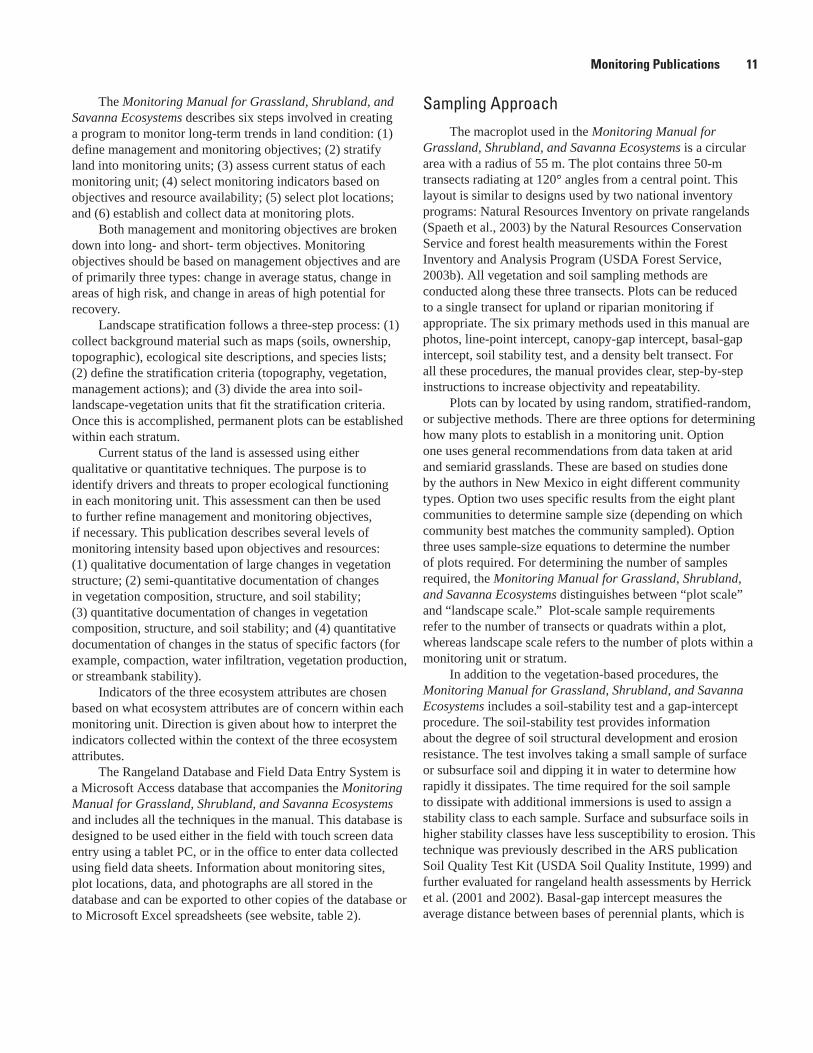
Sampling ApproachThe macroplot used in the Monitoring Manual for

Grassland, Shrubland, and Savanna Ecosystems is a circular area with a radius of 55 m. The plot contains three 50-m transects radiating at 120° angles from a central point. This layout is similar to designs used by two national inventory programs: Natural Resources Inventory on private rangelands (Spaeth et al., 2003) by the Natural Resources Conservation Service and forest health measurements within the Forest Inventory and Analysis Program (USDA Forest Service, 2003b). All vegetation and soil sampling methods are conducted along these three transects. Plots can be reduced to a single transect for upland or riparian monitoring if appropriate. The six primary methods used in this manual are photos, line-point intercept, canopy-gap intercept, basal-gap intercept, soil stability test, and a density belt transect. For all these procedures, the manual provides clear, step-by-step instructions to increase objectivity and repeatability.

Plots can by located by using random, stratified-random, or subjective methods. There are three options for determining how many plots to establish in a monitoring unit. Option one uses general recommendations from data taken at arid and semiarid grasslands. These are based on studies done by the authors in New Mexico in eight different community types. Option two uses specific results from the eight plant communities to determine sample size (depending on which community best matches the community sampled). Option three uses sample-size equations to determine the number of plots required. For determining the number of samples required, the Monitoring Manual for Grassland, Shrubland, and Savanna Ecosystems distinguishes between “plot scale” and “landscape scale.” Plot-scale sample requirements refer to the number of transects or quadrats within a plot, whereas landscape scale refers to the number of plots within a monitoring unit or stratum.

In addition to the vegetation-based procedures, the Monitoring Manual for Grassland, Shrubland, and Savanna Ecosystems includes a soil-stability test and a gap-intercept procedure. The soil-stability test provides information about the degree of soil structural development and erosion resistance. The test involves taking a small sample of surface or subsurface soil and dipping it in water to determine how rapidly it dissipates. The time required for the soil sample to dissipate with additional immersions is used to assign a stability class to each sample. Surface and subsurface soils in higher stability classes have less susceptibility to erosion. This technique was previously described in the ARS publication Soil Quality Test Kit (USDA Soil Quality Institute, 1999) and further evaluated for rangeland health assessments by Herrick et al. (2001 and 2002). Basal-gap intercept measures the average distance between bases of perennial plants, which is

Monitoring Publications 11

an indicator of susceptibility to erosion. These procedures can be used in conjunction with vegetation cover data to determine the risk of exposed soil to water erosion.

Fire Effects Monitoring and Inventory Protocol (Lutes et al., �00�)

The Fire Effects Monitoring and Inventory Protocol (FIREMON) is a monitoring system developed based on the NPS Fire Monitoring Handbook and a previous monitoring system called ECODATA. The purpose of FIREMON is to measure the effects of fire on critical ecosystem characteristics and to evaluate the impacts on ecosystem health and integrity.

FIREMON includes a recommended monitoring approach, fuels and vegetation sampling protocols, a Microsoft Access database, and a landscape-scale assessment method to quantify fire effects. The techniques in the manual are designed to assess the effects of wildland and prescribed fire as well as document the current state of a particular area.

Monitoring Program DesignFIREMON uses an “integrated sampling strategy”

that integrates monitoring goals and available resources to arrive at an acceptable sampling design. The strategy involves developing objectives and spatial stratification, plus determining sampling resources, approach, and intensity. First, goals and objectives of the monitoring program are formulated. Goals are described as broad statements of desired results whereas objectives are more narrowly focused. The FIREMON manual encourages objectives that are specific, measurable, achievable, relevant, and time-based.

Once objectives are selected, the sample area is stratified into homogeneous monitoring types or strata, resulting in a set of potential polygons to sample. Strata can be delineated by stand type, aspect, slope, fuels or other factors of interest to management. The criteria for defining strata should be linked to the objectives formulated for the monitoring project.

After the number of polygons in each strata is determined, the available resources for sampling are calculated. Determining the sampling resources consists of assessing available personnel, vehicles, and time to produce an estimate of the number of plots at which data collection can occur. Knowledge of the objectives, areas that need to be monitored, and resources available are then assessed to determine the appropriate sampling approach.

Sampling ApproachThere are two main sampling approaches within

FIREMON, relevé (qualitative) and statistical. The relevé method is applied when there are clearly not enough resources

to sample in a way that would be adequate for a statistical analysis. This method is used mainly as a descriptive method or inventory. The statistical approach is used when there are enough resources to sample in a statistically adequate manner.

The authors recommend three potential sampling intensities: simple, alternative, and detailed. The simple sampling scheme is used when the number of plots that can be established is one-half or fewer than the number of plots needed and can only use the relevé method. The alternative sampling scheme is a balance between the simple and detailed monitoring intensities and can use either the relevé or statistical approach. The detailed sampling intensity generally uses the statistical approach. The goal of the detailed sampling intensity is to sample all polygons.

The first step in any of these sampling intensities is to determine how many samples are possible given the resources available. This is determined by assessing the time and resources available to the monitoring project. Using this information, the sampling approach and intensity can be adjusted to fit the resources. Once the sampling approach is determined and plot locations decided upon, the user chooses which techniques to use at each plot. The FIREMON methods generally use a 20- x 20-m macroplot within which transects are randomly located along and perpendicular to the baseline of the macroplot. Macroplot size can change depending on the technique and the needs of the user.

All field forms for collecting data are included in the FIREMON manual and all data collected at a particular site are linked by a plot description form, which includes background data as well as geographic coordinates for each plot. Observers fill out appropriate datasheets in the field and enter data into the FIREMON Microsoft Access database at the office.

Techniques in FIREMON are not strict – the user has the option to modify them and the database will accommodate many types of changes. Any changes to published techniques, as well as any information from the monitoring design process (such as objectives or problems encountered), are documented in a section of the database for metadata. The FIREMON database accepts all the data for the techniques in the manual, including tree density and size, fuel loading, cover/frequency, line intercept, point intercept and point frames, density belts and quadrats, rare species transects, and fire behavior (table 3).

Fuel and Fire Effects Monitoring Guide (USDI Fish and Wildlife Service, 1999)

The objective of the USFWS Fuel and Fire Effects Monitoring Guide (FFEMG) is to integrate fuel treatments and fire effects monitoring into refuge management plans. This manual draws heavily from the concepts and advice found in Measuring and Monitoring Plant Populations and Sampling Vegetation Attributes.

1� Monitoring Post-Fire Vegetation Rehabilitation Projects

Monitoring Program DesignThe monitoring program description from Measuring

and Monitoring Plant Populations is largely reproduced in the Fuel and Fire Effects Monitoring Guide. However, the Fuel and Fire Effects Monitoring Guide also deals with topics specific to fire effects, such as fuels, wildlife habitat, water, soil, and air, in addition to vegetation.

Sampling ApproachThe sampling approach found in the Fuel and Fire

Effects Monitoring Guide is similar to those used for Sampling Vegetation Attributes and includes the baseline, macroplot, and linear study designs. Study plots are placed in key areas, and inferences can only be applied to the area of the study.

Vegetation monitoring techniques described in the Fuel and Fire Effects Monitoring Guide are primarily derived from Sampling Vegetation Attributes. These include pace frequency, single and nested quadrat frequency, dry-weight rank, Daubenmire cover, line intercept, point intercept, and vegetation structure (cover board and Robel pole).

Additional techniques are included for sampling water quality (temperature, pH, turbidity, etc.), air quality (smoke), and hydrophobicity of soils.

Range and Training Land Assessment Technical Reference Manual (U.S. Army, �00�)

The RTLA Technical Reference Manual (RTLA) was developed by the U.S. Army for monitoring military land. The RTLA is a comprehensive compilation of techniques for vegetation monitoring and also includes a database used to store data. The original RTLA (formerly called LCTA, Land Condition Trend Analysis) was a prescriptive manual, but as the program progressed, different methodologies were found to work better at installations in different ecoregions, and specific methods were no longer mandated. The authors ask that it be viewed as a collection of information rather than a step-by-step guide.

Monitoring Program DesignMuch like the other manuals, the RTLA describes the

general monitoring topics such as the purpose, development and use of conceptual models, level and intensity, management and monitoring objectives, and variable selection. The RTLA also discusses the advantages of having well-written monitoring protocols covering all aspects of the program as well as a long-term monitoring plan.

Sampling principles are discussed in chapter three, including accuracy and precision, sampling and non-sampling errors, hypothesis testing, power analysis, biological significance, minimum detectable change, and statistical tests. The RTLA also discusses sampling design factors such as choosing the appropriate sampling unit, size and shape of sample units, sample placement, and sample-size requirements.

Sampling ApproachCurrently, the RTLA does not recommend a specific

sampling approach; however, the original LCTA recommended stratified random sampling with a plot density of one plot per 200 hectares.

The plot designs described in the manual are baseline, macroplot, and linear. The primary methods described in the manual measure vegetation frequency, cover, density, and biomass. The RTLA describes how to collect data using each method along with their applicability, advantages, and limitations. The manual further describes the sampling process using these techniques, data summary, and analysis.

There are no soil-erosion monitoring techniques discussed in the RTLA, but there is a discussion of soil-erosion equations (Universal Soil Loss Equation[USLE]), Revised USLE (RUSLE), Water Erosion Prediction Project (WEPP), and Wind Erosion Equation (WEQ). These can be used to estimate the amount of erosion provided some basic information about each site is known, including percent plant cover, ground cover, and average canopy height.

The RTLA presents a detailed discussion of analysis and interpretation of monitoring data. This covers many of the same topics highlighted in the other vegetation monitoring manuals, including assumptions, confidence intervals, significance, and hypothesis testing. RTLA also presents examples of basic analysis of monitoring data depending on the situation, including parametric and non-parametric tests.

The RTLA describes many techniques that can be used to measure vegetation in both non-forested and forested ecosystems (table 3).

National Assessment ProgramsThere are two assessment programs that seek to

determine the state of natural resources on a national scale. Both programs use a statistical sampling scheme whereby inferences can be made at various spatial scales. In order to accomplish this, both programs have standardized procedures to ensure comparable data are collected at all plots, plus rigorous observer training and data-quality assurance programs.

National Assessment Programs 1�

National Resources Inventory (NRI)

The NRI is conducted by the Natural Resources Conservation Service (NRCS) in conjunction with the Iowa State University Statistical Laboratory. The NRI is designed to analyze primarily farmland and rangeland at local, state, and national levels from data collected at the plot level.

The NRI uses a stratified two-stage sampling method to select sampling units on non-federal land across the nation. First-stage sampling units (primary sample unit, PSU) are areas of land selected randomly from the approximately 300,000 eligible land parcels across the country. Second-stage sampling units are points randomly located within the primary sampling units.

Data collection occurs on both the PSUs and the sample points. At the PSUs, general data are collected such as information on types and acreages of farms, urban areas, water, and transportation uses. Within each PSU further detailed data collection is conducted. Point-data collections include ownership, soils, land-use and cover data, irrigation, wetlands, and erosion prediction equations. All data are collected according to standard protocols resulting in scientifically credible information about the status of natural resources on these lands.

In addition to the NRI, special field studies have been implemented to address areas of concern. In 2003, the “Rangeland Field Study” was implemented in 17 states west of the Mississippi. This study used the same NRI process with additional data collection to examine the state of private rangelands. Several new techniques were added to the inventory to accommodate this goal. New data collected included ecological site information, rangeland health, noxious weeds, disturbance indicators, and the quantitative techniques of soil stability test, line-point transects, canopy and basal-gap transects, and cover pole (vegetation structure).

In the field, qualitative and quantitative data are collected using a database program on a pocket PC called the Computer Assisted Survey Instrument (CASI). Once data are collected, they can be transferred to a central repository via the CASI. Data analysis is then conducted to create an overall assessment of the state of these lands.

Forest Inventory and Analysis (FIA) (USDA Forest Service, �00�b)

The FIA is a census of the nation’s forest resources, regardless of ownership, conducted by the USFS. The FIA program collects plot-level data that are used to generate a national assessment of forest health. The FIA uses a set of core methods collected on a standard plot that are analyzed and reported in a similar manner nationwide. Regions must follow the core methods but may include additional methods.

The FIA consists of three phases of differing spatial scales. Phase one includes remote sensing and satellite

imagery to classify forested and non-forested areas. Phase two includes forest-survey field-data collection plots located approximately every 6,000 acres, 10 percent of which are visited each year. Phase three consists of a subsample of phase two plots of which 20 percent are sampled each year (one per 100,000 acres) and attributes specifically related to forest health are measured.

General data collected for phase two FIA plots include characteristics such as location information, condition class, forest type, regeneration status, tree and seedling density, and understory vegetation description. Phase three measurements include crown conditions, woody debris, lichens, ozone damage, and soils. Soils information collected on phase three plots includes soil erosion, soil compaction, and soil chemistry. On FIA plots, soil erosion is estimated using established models, such as the RUSLE, and by collecting information on bare soils in each subplot. Soil samples also are taken for laboratory analysis.

The FIA program includes standardized training and certification of all crew members as well as quality control using in-the-field audits, re-checking of sample plots, and the use of data recorders.

Common Elements of Monitoring Program Designs

Many elements of monitoring program design and sampling approaches used in the monitoring manuals reviewed could be implemented in a common monitoring approach to evaluate ES&R treatment effectiveness. The following are descriptions of program design elements found within the reviewed monitoring manuals that are suitable for use in evaluating ES&R treatment success (table 3). See Appendix B for examples of projects using these elements.

Objectives

All seven monitoring manuals reviewed in this report included objectives as an important component of a monitoring program. Several of the manuals provide good descriptions of how to formulate objectives. As described in Measuring and Monitoring Plant Populations, both management and sampling objectives should be written for any project. Management objectives are “clearly articulated descriptions of a measurable standard, desired state, threshold value, amount of change, or trend that you are striving to achieve for a particular plant population or habitat characteristics.” Well-defined management objectives in a monitoring program perform two functions: first, they establish a standard to measure the degree of success; and second, they determine the appropriate indicators to measure. A standard protocol can then be followed for the measurement


of each indicator; thus, data-collection activities are directly related to management objectives. Sampling objectives should be paired with each management objective and specify the desired confidence level, confidence interval width (precision), level of type II error, or detectable change for the sampling effort. Examples of management and sampling objectives are provided in Appendix B, as well as in the monitoring manuals reviewed.

Stratification

Stratification is described in five of the seven monitoring manuals reviewed. Stratification is the partitioning of treatment areas to reduce variation and increase precision of sampling efforts. Areas that may respond differently to ES&R treatments such as different soil types or ecological sites are good candidates for strata. Rules for stratification of treatment areas into monitoring units should be created during the planning stage of an ES&R project. Stratification can be undertaken concurrently with or after identification of treatment areas. In many cases, stratification is completed as a byproduct of treatment planning such as assigning different seed mixes to sites with different characteristics or potentials.

Background information on the treatment area is essential for stratification (Herrick et al., 2005b; Lutes et al., 2006; USDI NPS, 2003). A variety of GIS data are useful for delineating monitoring units, including digital elevation models (DEMs), fire perimeters, proposed and actual treatment areas, soils (if available), roads, and land-use information. Using GIS software, such as ArcGIS, monitoring units can be derived based on the available information and the specifics of the project. If shapefiles for ecological sites are available, then these files may be the preferred initial strata. If only soils are available, then the site can be divided initially into soil strata separately to reduce variation and increase monitoring efficiency. If shapefiles are available for only soils, but soil-to-ecological site correlations are known, then differing soils that correlate to the same ecological site may be combined into the same strata. Additionally, slope classes can be generated from DEMs when seedings will occur over a large range of slopes. Areas that are not likely to be seeded due to topography can be excluded from the monitoring unit using DEMs.

Using this information, stratification of the area for both treatments and monitoring can be accomplished using a defined set of variables such as slope, aspect, elevation, treatment type, minimum size, soil type, or ecological site.

Descriptions of monitoring units should be included in monitoring plans so that the scope of inference is known. For example:

Monitoring unit 1 includes all areas of less than 20 percent slope within soil type A in the native seed mix treatment.

•

Monitoring unit 2 includes all areas equal to or greater than 20 percent slope within soil type A in the native seed mix treatment.

Monitoring unit 3 includes all areas of less than 20 percent slope within the non-native seed mix treatment.

Similar methods of stratification used on different projects will facilitate comparisons among those projects and aid region-wide assessments of ES&R treatment effectiveness. Additional information on stratification can be found in the Fire Monitoring Handbook (USDI NPS, 2003), Fire Effects Monitoring and Inventory Protocol (Lutes et al., 2006), and the Monitoring Manual for Grassland, Shrubland, and Savanna Ecosystems (Herrick et al., 2005b).

Controls

Control plots are locations within a proposed treatment area that are established prior to and avoided when treatments are implemented. Control plots are mentioned in two of the seven monitoring manuals reviewed (FIREMON and the Fire Monitoring Handbook), however their purpose and description in these manuals do not match the goal of determining treatment effectiveness of ES&R projects. Both manuals state that control plots are placed outside the perimeter of a prescribed burn and do not require them depending on where a particular project falls within the monitoring-research continuum. The Fire Monitoring Handbook states that control areas should be used when attributing a particular effect to the applied treatment. This is the situation that occurs when evaluating the effects of ES&R treatment because the goal is to show that the treatment caused the observed change. In the absence of control plots, comparing treatment areas to established quantitative objectives is the best way to determine treatment effectiveness.

Placement of control plots is an important pre-treatment activity. Control plots should be randomly placed within each monitoring unit. Control plots should not be placed in adjacent untreated areas because, presumably, the untreated areas are different from treated areas. Additionally, because control plots must be set up before treatment, it is not possible to know exactly how many are required. However, a minimum of three control plots should be established within any monitoring unit. Control plots also provide important information on natural recovery that can be used to determine whether or not treatments were necessary in the first place. This is especially useful given limited resources for implementing large projects in severe fire years.

Control plots may not be practical in all situations. For instance, in situations where life and property values are threatened (for example, slopes above developments) or when it would be very difficult to not treat an area (for example, aerial seeding). However, controls should be used whenever possible because they provide the best measure of natural regeneration and ES&R treatment success.

•

•

Common Elements of Monitoring Program Designs 1�

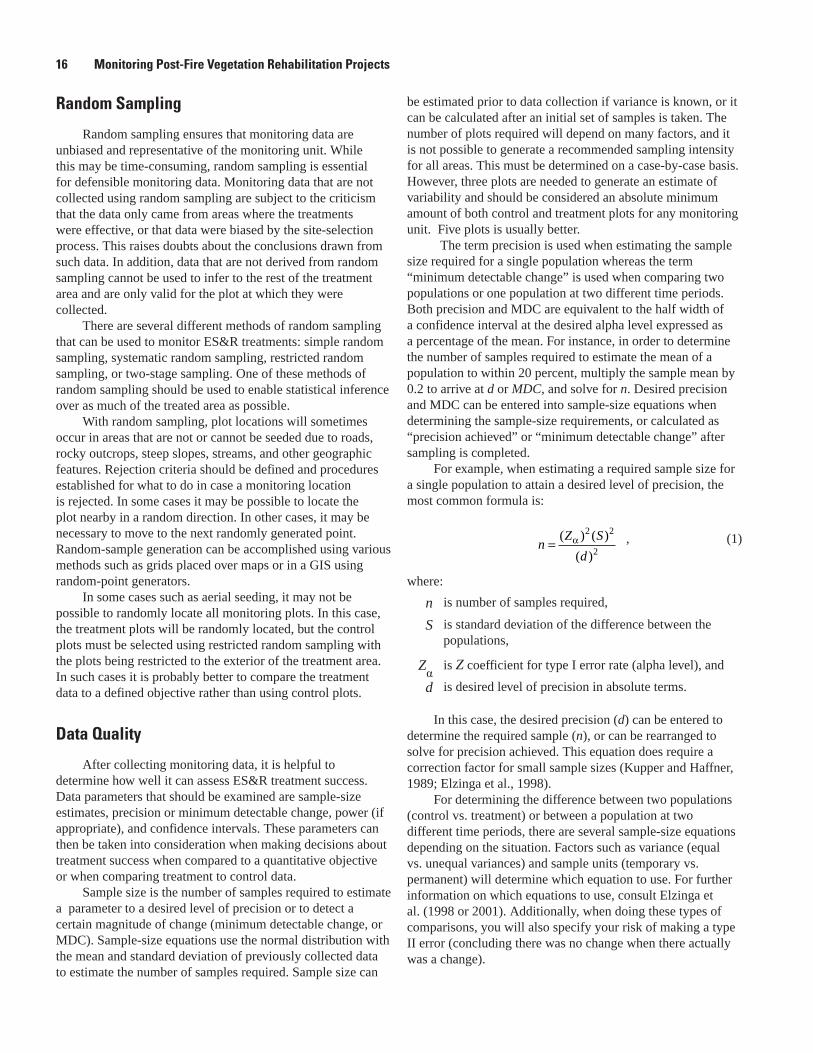
Random Sampling

Random sampling ensures that monitoring data are unbiased and representative of the monitoring unit. While this may be time-consuming, random sampling is essential for defensible monitoring data. Monitoring data that are not collected using random sampling are subject to the criticism that the data only came from areas where the treatments were effective, or that data were biased by the site-selection process. This raises doubts about the conclusions drawn from such data. In addition, data that are not derived from random sampling cannot be used to infer to the rest of the treatment area and are only valid for the plot at which they were collected.

There are several different methods of random sampling that can be used to monitor ES&R treatments: simple random sampling, systematic random sampling, restricted random sampling, or two-stage sampling. One of these methods of random sampling should be used to enable statistical inference over as much of the treated area as possible.

With random sampling, plot locations will sometimes occur in areas that are not or cannot be seeded due to roads, rocky outcrops, steep slopes, streams, and other geographic features. Rejection criteria should be defined and procedures established for what to do in case a monitoring location is rejected. In some cases it may be possible to locate the plot nearby in a random direction. In other cases, it may be necessary to move to the next randomly generated point. Random-sample generation can be accomplished using various methods such as grids placed over maps or in a GIS using random-point generators.

In some cases such as aerial seeding, it may not be possible to randomly locate all monitoring plots. In this case, the treatment plots will be randomly located, but the control plots must be selected using restricted random sampling with the plots being restricted to the exterior of the treatment area. In such cases it is probably better to compare the treatment data to a defined objective rather than using control plots.

Data Quality

After collecting monitoring data, it is helpful to determine how well it can assess ES&R treatment success. Data parameters that should be examined are sample-size estimates, precision or minimum detectable change, power (if appropriate), and confidence intervals. These parameters can then be taken into consideration when making decisions about treatment success when compared to a quantitative objective or when comparing treatment to control data.

Sample size is the number of samples required to estimate a parameter to a desired level of precision or to detect a certain magnitude of change (minimum detectable change, or MDC). Sample-size equations use the normal distribution with the mean and standard deviation of previously collected data to estimate the number of samples required. Sample size can

be estimated prior to data collection if variance is known, or it can be calculated after an initial set of samples is taken. The number of plots required will depend on many factors, and it is not possible to generate a recommended sampling intensity for all areas. This must be determined on a case-by-case basis. However, three plots are needed to generate an estimate of variability and should be considered an absolute minimum amount of both control and treatment plots for any monitoring unit. Five plots is usually better.

The term precision is used when estimating the sample size required for a single population whereas the term “minimum detectable change” is used when comparing two populations or one population at two different time periods. Both precision and MDC are equivalent to the half width of a confidence interval at the desired alpha level expressed as a percentage of the mean. For instance, in order to determine the number of samples required to estimate the mean of a population to within 20 percent, multiply the sample mean by 0.2 to arrive at d or MDC, and solve for n. Desired precision and MDC can be entered into sample-size equations when determining the sample-size requirements, or calculated as “precision achieved” or “minimum detectable change” after sampling is completed.

For example, when estimating a required sample size for a single population to attain a desired level of precision, the most common formula is:

nZ S

d=

( ) ( )( )

α2 2

2 , (1)

where:

n is number of samples required,

S is standard deviation of the difference between the populations,

Zα is Z coefficient for type I error rate (alpha level), and

d is desired level of precision in absolute terms.

In this case, the desired precision (d) can be entered to determine the required sample (n), or can be rearranged to solve for precision achieved. This equation does require a correction factor for small sample sizes (Kupper and Haffner, 1989; Elzinga et al., 1998).

For determining the difference between two populations (control vs. treatment) or between a population at two different time periods, there are several sample-size equations depending on the situation. Factors such as variance (equal vs. unequal variances) and sample units (temporary vs. permanent) will determine which equation to use. For further information on which equations to use, consult Elzinga et al. (1998 or 2001). Additionally, when doing these types of comparisons, you will also specify your risk of making a type II error (concluding there was no change when there actually was a change).


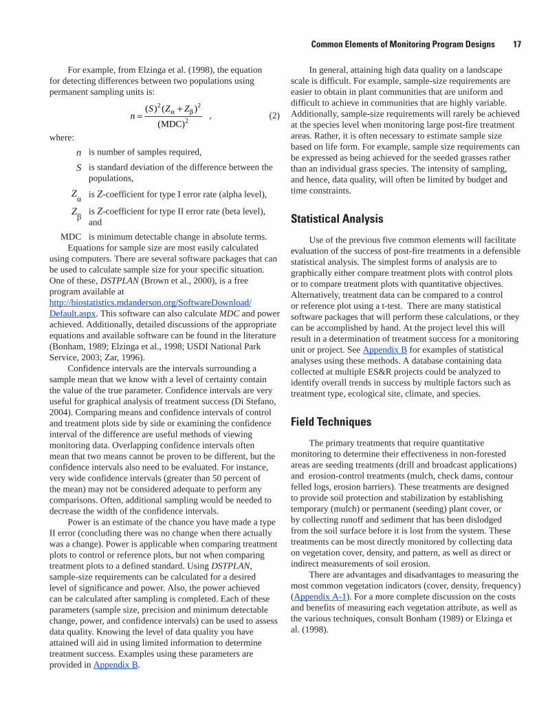
For example, from Elzinga et al. (1998), the equation for detecting differences between two populations using permanent sampling units is:

nS Z Z

=+( ) ( )

( )

2 2

2α β

MDC , (2)

where:


S is standard deviation of the difference between the populations,

Zα is Z-coefficient for type I error rate (alpha level),

Zβ is Z-coefficient for type II error rate (beta level), and

MDC is minimum detectable change in absolute terms.Equations for sample size are most easily calculated

using computers. There are several software packages that can be used to calculate sample size for your specific situation. One of these, DSTPLAN (Brown et al., 2000), is a free program available at http://biostatistics.mdanderson.org/SoftwareDownload/Default.aspx. This software can also calculate MDC and power achieved. Additionally, detailed discussions of the appropriate equations and available software can be found in the literature (Bonham, 1989; Elzinga et al., 1998; USDI National Park Service, 2003; Zar, 1996).

Confidence intervals are the intervals surrounding a sample mean that we know with a level of certainty contain the value of the true parameter. Confidence intervals are very useful for graphical analysis of treatment success (Di Stefano, 2004). Comparing means and confidence intervals of control and treatment plots side by side or examining the confidence interval of the difference are useful methods of viewing monitoring data. Overlapping confidence intervals often mean that two means cannot be proven to be different, but the confidence intervals also need to be evaluated. For instance, very wide confidence intervals (greater than 50 percent of the mean) may not be considered adequate to perform any comparisons. Often, additional sampling would be needed to decrease the width of the confidence intervals.

Power is an estimate of the chance you have made a type II error (concluding there was no change when there actually was a change). Power is applicable when comparing treatment plots to control or reference plots, but not when comparing treatment plots to a defined standard. Using DSTPLAN, sample-size requirements can be calculated for a desired level of significance and power. Also, the power achieved can be calculated after sampling is completed. Each of these parameters (sample size, precision and minimum detectable change, power, and confidence intervals) can be used to assess data quality. Knowing the level of data quality you have attained will aid in using limited information to determine treatment success. Examples using these parameters are provided in Appendix B.

In general, attaining high data quality on a landscape scale is difficult. For example, sample-size requirements are easier to obtain in plant communities that are uniform and difficult to achieve in communities that are highly variable. Additionally, sample-size requirements will rarely be achieved at the species level when monitoring large post-fire treatment areas. Rather, it is often necessary to estimate sample size based on life form. For example, sample size requirements can be expressed as being achieved for the seeded grasses rather than an individual grass species. The intensity of sampling, and hence, data quality, will often be limited by budget and time constraints.

Statistical Analysis

Use of the previous five common elements will facilitate evaluation of the success of post-fire treatments in a defensible statistical analysis. The simplest forms of analysis are to graphically either compare treatment plots with control plots or to compare treatment plots with quantitative objectives. Alternatively, treatment data can be compared to a control or reference plot using a t-test. There are many statistical software packages that will perform these calculations, or they can be accomplished by hand. At the project level this will result in a determination of treatment success for a monitoring unit or project. See Appendix B for examples of statistical analyses using these methods. A database containing data collected at multiple ES&R projects could be analyzed to identify overall trends in success by multiple factors such as treatment type, ecological site, climate, and species.

Field Techniques

The primary treatments that require quantitative monitoring to determine their effectiveness in non-forested areas are seeding treatments (drill and broadcast applications) and erosion-control treatments (mulch, check dams, contour felled logs, erosion barriers). These treatments are designed to provide soil protection and stabilization by establishing temporary (mulch) or permanent (seeding) plant cover, or by collecting runoff and sediment that has been dislodged from the soil surface before it is lost from the system. These treatments can be most directly monitored by collecting data on vegetation cover, density, and pattern, as well as direct or indirect measurements of soil erosion.

There are advantages and disadvantages to measuring the most common vegetation indicators (cover, density, frequency) (Appendix A-1). For a more complete discussion on the costs and benefits of measuring each vegetation attribute, as well as the various techniques, consult Bonham (1989) or Elzinga et al. (1998).

Common Elements of Monitoring Program Designs 1�

http://biostatistics.mdanderson.org/SoftwareDownload/Default.aspx


CoverPlant cover acts to protect soil from the energy of falling

raindrops, wind, and surface runoff (Morgan, 2005). The amount of cover of desirable and undesirable species, as well as soil-surface cover can be used to evaluate the effectiveness of post-fire treatments. Comparisons of treated areas to control areas can provide information on the magnitude and direction of treatment effects. There are several types of cover that can be measured: basal cover (the area covered by plant bases), foliar cover (the area covered by both basal and aerial plant parts), canopy cover (the area covered by drawing a line around the perimeter of the aerial portions of a plant), and total cover (proportion of the soil surface covered by aerial and basal vegetation, litter, rocks, and microbiota).

There are several different methods of measuring cover, including visual estimation (for example, Daubenmire canopy cover classes), line intercepts, point intercepts, and plotless methods. Visual estimation involves estimating the percent canopy cover of vegetation within a quadrat. Visual estimations are usually made by class rather than exact percentages. Visually estimating the percent cover within a quadrat is considered a semi-quantitative technique by Bonham (1989). Line intercepts involve measuring the linear distance of a transect that is covered by perennial species. Point intercept involves placing a pin or group of pins along a transect and recording the species and substrates intercepted. Point intercepts have been shown to be more efficient and objective than either visual estimation methods or line intercepts (Floyd and Anderson, 1987; Bonham, 1989) (Appendix A-2). Basal, foliar, and total cover can be estimated for annuals, herbaceous perennials, and shrubs using the point-intercept technique, whereas the line-intercept technique measures only canopy cover and is not well suited for annual species (Appendix A-2). Plotless methods involve using a sighting device to count plants within a variable radius around a plot center. Plotless methods for measuring cover and density are more applicable to measuring shrubs and trees and are not as useful for herbaceous species. Plotless methods may be suitable at sites with mature shrubs and trees, but this situation would not likely occur during the three-year post-fire monitoring period.

Some factors that can affect the collection of cover data are plant morphology, wind, and observer error. Plants that have flat leaves tend to be intercepted more often with a pin lowered at 90º than plants that have inclined leaves (such as grasses), however, this is acceptable when the primary concern is soil stabilization rather than light interception. When using cover to assess dominance and diversity, inclined pins may be more appropriate. Wind may move aerial plant parts, causing

them to touch intercept devices more often, leading to higher cover estimates. This can lead to observer errors if attention is not paid to whether or not the plant part was touching the point intercept just as the intercept was lowered. Other observer errors can be failure to maintain the point intercept at the proper angle (90°), and not bending down close enough to see lower plants and soil surfaces.

DensityDensity can be used to evaluate the effectiveness of

post-fire treatments by showing the change in the number of desirable or undesirable plants per unit area. There are several quantitative methods to collect density data. The most common and repeatable measurement of density is counting the number of plants in a known area. This method is an objective measure that can be compared between different sites. Plotless methods, which involve measuring the distance between plant bases or between sample points and plant bases, are also used. Distance measurements are then used to calculate the mean area per plant, the reciprocal of which is density.

There are several issues that must be addressed when measuring density with quadrats. First, the size and shape of the quadrat are important to efficiency of the sampling effort. The size and shape of the quadrat influences the variability in the resulting data. If a quadrat is too small, there will be a high percentage of zeros resulting in a high degree of variability in the data, necessitating the collection of additional samples. If the quadrat is too large, the observer will spend more time than necessary collecting data at each sample location, resulting in higher cost for the monitoring effort. Second, what constitutes an individual plant must be clearly defined. This is especially true in the case of rhizomatous or multi-stemmed species, or in the case where plants occur so close together that it is difficult to determine the boundaries among individuals. Strict definitions of what is to be counted must be defined and followed during monitoring. Third, the problem of mass die-offs can obscure what is happening in a plant community unless size or age classes are tracked. For example, seedlings often emerge in large numbers after a seeding but few may survive to the next year. If seedlings are not counted separately from adults, the resulting density trend may be misleading. Fourth, when monitoring seeded treatments, plant size is expected to change from seedling to established plant during the three-year monitoring period. This means that different quadrat sizes may be needed in different years to efficiently sample the area. Fifth, rules for counting plants that are near the boundary of the quadrat must be defined and consistently followed.


Gap InterceptGap intercept measurements are a recent addition to

vegetation attributes and are related to ES&R objectives because the percentage of large gaps within a community is associated with site stability, biotic integrity, and hydrologic function (Herrick et al., 2005b). Two types of gap measurements can be made, canopy and basal. Canopy gaps measure the percent of the transect that is not covered by plant canopy, whereas basal gaps measure the distance between the bases of perennial plant species along the transect. The percentage of each transect occupied by each class of gap sizes is calculated for the transect. Canopy-gap measurements are related to wind erosion and are slightly less repeatable, whereas basal-gap measurements are related to water erosion.

The percentage of large basal gaps is representative of the spatial heterogeneity of the plant community, and this measurement has been correlated with risk of soil erosion and degradation of ecosystems (Schlesinger et al., 1990; de Soyza et al., 1997; Herrick et al., 2002). Changes can occur in the percentage and size of gaps while both cover and density measurements remain stable. The higher the proportion of the transect that contains large gaps, the higher the risk of erosion by wind or water, and the more susceptible the site is to invasions by exotic species. Following ES&R treatments, the percentage of the community covered by large gaps should decrease with time.

Basal-gap measurements are objective and easy to collect. In addition, they are highly repeatable when conducted along permanent transects and show little variability from year to year due to environmental factors. The procedure is relatively fast because the species of each individual plant base does not need to be determined. However, this can be done to help separate the effects of seedings from natural recovery, adding time to the procedure. Measurements are typically fast in sparsely vegetated plant communities but take additional time in dense vegetation.

Non-Standard TechniquesTwo vegetation attributes that are not considered for

use in this report are frequency and production. Frequency is the easiest vegetation attribute to measure, but it is the most difficult to interpret because it is not an absolute measure of a plant community (Bonham, 1989). Most of the difficulty derives from the fact that frequency data are highly dependent on the shape and size of the quadrat used and the spatial distribution of the plants in the community being measured. Different species and plant communities require differing quadrat shapes and sizes. Therefore, comparisons are only valid when exactly the same shape and size of quadrats are used. For this reason, frequency is difficult to compare across

projects and should only be used in specific situations where sites are consistent enough to use the same plot size and shape, or where no comparisons will be made. For instance, frequency may be an important attribute to detect weed invasion. Production techniques are also not included because they are time-consuming and relate less directly to soil protection and stabilization than cover measurements.

Erosion MonitoringNumerous methods have been devised to directly and

indirectly measure soil erosion due to water. Two field methods that are applicable to non-forested upland include an indirect measure of the change in elevation of the soil surface and a direct measure of the sediment produced from a defined area. Many other techniques have been developed that are highly sophisticated and are primarily suitable for research.

Elevational techniques used in the field are generally pins and bridges (Morgan, 2005). Erosion pins involve placing a pin or rod into the soil and measuring the location of the surface of the soil on the pin. Changes in elevation of the surface of the soil on the pin indicate soil erosion or deposition. The amount of soil lost or gained can then be estimated using the change in elevation and the bulk density of the soil. Erosion bridges are similar except that these utilize two pins on which a bridge rests. Measurements of soil elevation are made by lowering a rod at several points along the bridge to the soil surface. Measurements are taken over time to determine if any soil has eroded from or been deposited at the site. This method is generally more accurate than erosion pins. Both techniques require that no movement of the equipment occurs due to frost heaving, animals, or other disturbances in order for the measurements to be accurate.

Direct measurement of sediment can be accomplished in a number of ways. Most common in the field are erosion troughs and silt fences. Erosion troughs measure the amount of sediment produced from a known area that accumulates over time in a trench in which a metal trough is placed. Periodically, observers scoop and measure the amount of sediment that has accumulated in the trough. Silt fences also trap sediment from a defined area. This technique involves placing several posts or stakes and attaching silt fence to them. The fence traps sediments as water flows through it during rainfall events. The sediment is collected after storm events to provide an estimate of soil loss. This method, originally described by Dissmeyer (1982), was improved upon by Robichaud and Brown (2002), including exact specifications and examples of how to perform statistical analyses. Because this method is a direct measurement of erosion it is often preferable to indirect measurements such as those with erosion pins or bridges.

Common Elements of Monitoring Program Designs 19

A Common Approach for Monitoring Future ES&R Treatments

A common approach is needed to address GAO concerns (GAO, 2003) and facilitate evaluation of multiple ES&R projects. The results of this overview suggest an approach that incorporates the six common program design elements. Also suggested are the consistent use of comparable field techniques within each ecoregion and plant community.

Objectives: determine what to measure, the desired outcome, and how to evaluate success

Stratification: defines the treatment areas into monitoring units that are less variable and may be compared across projects

Control areas: allow a direct measurement of treatment effect

Random sampling: enables statistical inference and analysis

Data quality: assesses how well the data will answer questions of treatment success

Statistical analysis: allows a defensible assessment of treatment success

The following quantitative techniques should minimize observer bias and inter-observer variation among years and projects.

Cover with single point intercepts along a transect

Density with quadrats

Basal gap intercept along a transect

Direct measurements of erosion with silt fence

These vegetation and erosion attributes are absolute measures of ecological condition and can be compared with data collected in other areas. Because of this, various parameters can be changed between projects to enhance sampling efficiency in response to variation without affecting data comparability. These parameters are: (1) quadrat size and shape; (2) transect length; and (3) number of points or quadrats per transect or plot. Additional quantitative and qualitative procedures can also be added to address other concerns for specific areas.

Additionally, using well-documented procedures that include specific rules along with observer training will increase the quality of the data. Certified data gatherers who have been trained and have passed a series of standard exercises will help to minimize errors using these methods, thereby making observers comparable among themselves, between sites, and throughout years to the highest degree possible. Evaluation of the effectiveness of various treatments

•

•

•

•

•

•

•

•

•

•

within an ecoregion and plant community will benefit by consistent monitoring procedures, resulting in improved adaptive management and increased knowledge of ecosystem response to post-fire rehabilitation methods for future ES&R projects.

This approach would help address GAO concerns by monitoring multiple projects with comparable methods, consistently documenting results, allowing for the creation of a central database for query and reporting, and ultimately determining the effectiveness of post-fire rehabilitation activities region-wide.

While some authors of the manuals reviewed as well as agency personnel have expressed concern with a standardized approach to monitoring (Elzinga et al., 1998; USDI Fish and Wildlife Service, 1999), the majority of manuals agree on what elements to include in a monitoring program. Additionally, manuals and personnel use the same basic techniques for vegetation and soil monitoring throughout the USDA and USDI. Because ES&R and BAER projects generally have specific objectives such as preventing the invasion or expansion of exotic species or increasing cover and density of perennial species to reduce soil erosion, standard protocols to address these common objectives within an ecoregion and plant community can be used. Level III ecoregions (derived from Omernik, 1987) or major Land Resource Area (MLRA) may be an appropriate level within which to standardize a monitoring approach.

Many of the criticisms for a standard monitoring protocol were listed in Elzinga et al. (1998) and can be addressed using the proposed approach. The following are four primary criticisms and responses resulting from the proposed approach:

1. Monitoring data collected using standardized techniques are not designed for all situations, and therefore lack the ability to answer a variety of land management objectives.

The approach we describe provides common elements and techniques designed to answer the limited objectives that are common to ES&R projects. However, it is not a one-size-fits-all approach; rather, it is a targeted approach defined by management actions, objectives, ecoregion, and plant community. There are no restrictions on additional monitoring for other objectives of particular interest to individual offices.

2. Standard techniques do not address issues of statistical precision and power; therefore, data may be too imprecise for management decisions.

The elements of stratification, data quality, and random sampling are included to specifically increase statistical precision and power when dealing with the limited objectives of ES&R treatments.

3. Many public groups are skeptical of data from standard agency techniques.

�0 Monitoring Post-Fire Vegetation Rehabilitation Projects

The approach we describe in this report utilizes techniques to increase objectivity and decrease bias (random sampling, statistical analysis, objective techniques). The use of this approach should have the effect of promoting public confidence in data collected by management agencies.

4. Because funding is limited, projects should be designed on a case-by-case basis to maximize efficiency.

It is true that funding is often limited and that monitoring can be very expensive. We suggest, as does the BLM, that monitoring should be commensurate with the importance of the fire in terms of size or severity. Very small fires may only need to be monitored qualitatively at low cost. For large fires where significant funds are expended on ES&R treatments, a more quantitative approach should be taken. Because a standardized approach for the design and implementation of the monitoring would be used, labor costs for conducting the monitoring should easily be projected. Once estimates of the time required to implement this monitoring approach are determined, the appropriate level of funding can be requested from the ES&R program when a monitoring plan is developed. If adequate personnel are not available to implement the monitoring project, contractors could be used to perform the monitoring after completing a certified training course.

Another common criticism of monitoring approaches such as this one that incorporates random sampling,

stratification, and controls is that monitoring is not research and should not be subjected to the same rigor. Elements commonly used in research have been used to improve monitoring programs and are advocated by land management personnel and agency monitoring manuals (fig. 2). According to Busch and Trexler (2003) “Research and monitoring exist in a continuum of scientific endeavor.” There are many similarities between an effective monitoring program and research. Essential factors in a monitoring program are: (1) well-defined objectives and procedures, (2) stratification (similar to blocking), (3) controls, (4) random sampling, (5) knowledge of the confidence, power, and precision obtained, and (6) statistical testing. These factors do push monitoring closer to the research side, but they also result in defensible monitoring data.

ConclusionsA monitoring strategy using common elements and

standard procedures implemented within an ecoregion for specific plant communities can be used to evaluate ES&R treatments and will maximize the utility of the resulting data. The described approach includes the common elements of objectives, stratification, random sampling, controls, data quality, and statistical analysis, combined with standard

Well-defined objectives

Stratification

Hypotheses

Controls (when used)

Random sampling

Sample size estimation

Confidence and precision

Statistical testing

Well-defined objectives

Stratification

Hypotheses

Blocking

Control

Random treatments

Treatment Replication

Random sampling

Sample size estimation

Confidence and precision

Statistical testingFigure �. Similarities between monitoring and research. Bold text indicates elements in common.

Conclusions �1

data-collection procedures, to facilitate statistically valid, comparable data at the project level.

When choosing techniques for use across an ecoregion by many individuals, the least subjective method is preferred. The most objective quantitative methods are point cover, density, gap intercept, and direct measurement of erosion. A central database containing comparable monitoring information on multiple projects within an ecoregion could be created and used to complete a regional assessment of the effectiveness of different ES&R techniques. Additionally, such a database could also be queried by land managers to answer questions for their specific locations and provide an invaluable long-term repository for monitoring information.

AcknowledgementsThis work was supported by the Bureau of Land

Management and the USGS Forest and Rangeland Ecosystem Science Center. We would also like to thank members of the project advisory board for helpful comments and suggestions on this report including: Jan Beyers (USFS), Jack Brown (BLM), Robert Burton (BLM), Mike Pellant (BLM), Pete Robichaud (USFS), Mitch Thomas (BLM), Brian Watts (BLM), and John Willoughby (BLM). We would also like to thank Jack Hamby, Randy Eyre, Sharon Paris, Tom Roberts, and Clif Fanning at the BLM. This manuscript was vastly improved by the comments from one anonymous reviewer and Matt Brooks (USGS). Thanks to John Ledges Ame for editing. Also, thanks to Manuela Huso and John Willoughby for statistical advice.

References

Beyers, J.L. 2004. Postfire seeding for erosion control: effectiveness and impacts on native plant communities. Conservation Biology 18(4):947-956.

Bonham, C.D. 1989. Measurements for terrestrial vegetation. John Wiley and Sons, New York. 338 p.

Brooks, M.L. 2005. Oral Communication. USGS – Western Ecological Research Station, Las Vegas Field Station. Las Vegas, NV.

Brown, B.W., Brauner, C., Chan, A., Gutierrez, D., Herson, J., Lovato, J., Polsley, J., Russell, K., Vernier, J. 2000. DSTPLAN, Version 1. University of Texas, M.D. Anderson Cancer Center, Department of Biomathematics. Houston, TX. http://biostatistics.mdanderson.org/SoftwareDownload/Default.aspx. Last accessed 9/20/06.

Busch, D.E., Trexler, J.C., eds. 2003. Monitoring ecosystems: interdisciplinary approaches for evaluating ecoregional initiatives. Island Press, Washington DC. 447 p.

Caplan, T. 2005. Oral Communication. Parametrix, Inc., Albuquerque, NM.

Dallal, G.E. PC-Size: Consultant - A program for sample-size determination. The American Statistician 44:243.

De Soyza, A.G., Whitford, W.G., Herrick, J.E. 1997. Sensitivity testing of indicators of ecosystem health. Ecosystem Health 3(1):44-53.

Di Stefano, J. 2004. A confidence interval approach to data analysis. Forest Ecology and Management 187:173-183.

Daubenmire, R. 1959. A canopy coverage method of vegetational analysis. Northwest Science 33:43-64.

Dissmeyer, G.E. 1982. How to use fabric dams to compare erosion from forestry practices. USDA, Forest Service, Southeast Areas. Forestry Rep. SA-FR-13. Atlanta, GA. 40 p.

Elzinga, C.L., Salzer, D.W., Willoughby, J.W. 1998. Measuring and Monitoring Plant Populations. USDI BLM Technical Reference 1730-1. National Business Center, Denver, CO. 492p.

Elzinga, C.L., Salzer, D.W., Willoughby, J.W., Gibbs, J. 2001. Monitoring plant and animal populations. Blackwell Science, Inc. London, England. 360 p.

Floyd, D.A., Anderson, J.E. 1987. A comparison of three methods for estimating plant cover. Journal of Ecology 75:221-228

GAO. Government Accountability Office. 2003. Wildland fires: better information needed on effectiveness of emergency stabilization and rehabilitation treatments. GAO-03-430. Washington, DC. 56 p.

Herrick, J.E., Whitford, W.G., de Soyza, A.G., Van Zee, J.W., Havstad, K.M., Seybold, C.A., Walton, M. 2001. Field soil aggregate stability kit for soil quality and rangeland health evaluations. Catena 44:27-35.

Herrick, J.E., Brown, J.R., Tugel, A.J., Shaver, P.L., Havstad, K.M. 2002. Application of soil quality to monitoring and management: paradigms from rangeland ecology. Agronomy Journal 94:3-11.

Herrick, J.E., Van Zee, J.W., Havstad, K.M., Burkett, L.M., Whitford, W.G. 2005a. Monitoring Manual for Grassland, Shrubland, and Savanna Ecosystems. Volume 1: quick start. USDA-ARS Jornada Experimental Range. Las Cruces, NM. 36 p.

Herrick, J.E., Van Zee, J.W., Havstad, K.M., Burkett, L.M., Whitford, W.G. 2005b. Monitoring Manual for Grassland, Shrubland, and Savanna Ecosystems. Volume 2: design, supplementary methods and interpretation. USDA-ARS Jornada Experimental Range. Las Cruces, NM. 200 p.

�� Monitoring Post-Fire Vegetation Rehabilitation Projects



Interagency Technical Reference. 1999. Sampling Vegetation Attributes. BLM Technical Reference 1734-4. National Business Center, Denver, CO. 158 p.

Janicki, A., Potter, D. 2003. Effects of grass seeding on post-fire erosion in a Sierra Nevada pine-hardwood community. USDA Forest Service, Pacific Southwest Region Stanislaus National Forest.

Kupper, L.L., Hafner, K.B. 1989. How appropriate are popular sample-size formulas? The American Statistician 43(2):101-105.

Lutes, Duncan C., Keane, Robert, E., Caratti, John. F., Key, Carl H., Benson, Nathan C., Sutherland, Steve, Gangi, Larry J., 2006. FIREMON: Fire Effects Monitoring and Inventory System. Gen. Tech. Rep. RMRS-GTR-164-CD. For Collins, CO: U.S. Department of Agriculture, Forest Service, Rocky Mountain Research Station. 1 CD. 400 p.

Morgan, R.P.C. 2005. Soil erosion and conservation. 3rd edition. Blackwell Publishing, Ltd., Oxford UK. 304 p.

Omernik, J.M. 1987. Ecoregions of the conterminous United States. Map (scale 1:7,500,000). Annals of the Association of American Geographers 77(1):118-125.

Pellant, M., Shaver, P., Pyke, D.A., Herrick, J.E. 2005. Interpreting the indicators of rangeland health (version 4). BLM Technical Reference 1734-6. United States Department of the Interior, Bureau of Land Management National Science and Technology Center, Denver CO. 122 p.

Peterson, D.A. 2005. Oral Communication. USFS PNW Res. Stn., Wenatchee Forestry Sciences Laboratory, Wenatchee, WA.

Pyke, D.A, McArthur, T.O. 2002. Emergency fire rehabilitation of BLM lands in the intermountain west: revegetation and monitoring. Interim Report to the BLM. 41 p.

Robichaud, P.R., Beyers, J.L., Neary, D.G. 2000. Evaluating the effectiveness of postfire rehabilitation treatments. USDA Forest Service, Rocky Mountain Research Station, Gen. Tech. Rep. RMR-S-GTR-63. Fort Collins CO. 85 p.

Robichaud, P.R., Brown, R.E. 2002. Silt fences: an economical technique for measuring hillslope soil erosion. USDA Forest Service, Rocky Mountain Research Station. Gen. Tech. Rep. RMRS-GTR-94. Fort Collins, CO. 24 p.

Schlesinger, W.H., Reynolds, J.F., Cunningham, G.L., Huenneke, L.J., Jarrell, W.M., Virginia, R.A., Whitford, W.G. 1990. Biological feedbacks in global desertification. Science 247(4946):1043-1048.

Spaeth, K.E., Pierson, F.B., Herrick, J.E., Shaver, P.L., Pyke, D.A., Pellant, M., Thompson, D., Dayton, R. 2003. New proposed national resources inventory protocols on nonfederal rangelands. Journal of Soil and Water Conservation 58(1):18-21.

The Nature Conservancy (TNC). 2005. Recovery and rehabilitation of vegetation on the Fitzner-Eberhardt Arid Lands Ecology Reserves, Hanford Reach National Monument, following the 24 Command Fire: final report 2001-2004. James R. Evans, Marita P. Lih. Seatle, WA. 289 p.

U.S. Army. Sustainable Range Program. 2006. RTLA Technical Reference Manual: Ecological Monitoring on Military Lands Draft. http://www.cemml.colostate.edu/itamtrm.htm. Accessed 10/21/06.

USDA Forest Service. 1995. Burned-area emergency rehabilitation handbook. Amendment No. 2509.13-95-3. http://www.fs.fed.us/cgi-bin/Directives/get_dirs/fsh?2509.13 Accessed 9/22/06.

USDA Forest Service. 2001. Soil quality monitoring methods, chapter 2: soil management handbook. FSH 2509.18. Intermountain Region handbook.

USDA Forest Service. 2003a. Rangeland ecosystem analysis and monitoring handbook. FSH 2209.21.

USDA Forest Service. 2003b. Forest inventory and analysis national core field guide. Volume 1: field data collection procedure for phase 2 plots, Version 1.7.

USDA Soil Quality Institute. 1999. Soil Quality Test Kit Guide. 82 p.

USDI. 2004. Wildland fire management burned area emergency stabilization and rehabilitation. Departmental Manual Part 620, Chapter 3.

USDI Bureau of Land Management. 2005. Emergency fire rehabilitation handbook. U.S. Department of the Interior, Bureau of Land Management Manual Handbook H-1742-1. Draft Dated April 7, 2005. 58 p.

USDI Fish and Wildlife Service. 1999. Fuel and Fire Effects Monitoring Guide. http://www.fws.gov/fire/downloads/monitor.pdf. Accessed 9/22/06.

USDI National Park Service. 2003. Fire Monitoring Handbook. Fire Management Program Center, National Interagency Fire Center. Boise, ID. 274p.

Zar, J.H. 1999. Biostatistical analysis, 3rd ed. Upper Saddle River, NJ. Prentice Hall.

References ��



http://www.fs.fed.us/cgi-bin/Directives/get_dirs/fsh?2509.13

http://www.fs.fed.us/cgi-bin/Directives/get_dirs/fsh?2509.13



Appe

ndix

es

Appe

ndix

A-1

Adva

ntag

es a

nd d

isad

vant

ages

of m

easu

ring

the

thre

e ba

sic

vege

tatio

n at

tribu

tes1

Cove

rDe

nsity

Freq

uenc

y

Desc

riptio

nT

he p

erce

ntag

e of

gro

und

cove

red

by v

eget

atio

n (f

olia

r, ba

sal,

grou

nd, t

otal

).D

ensi

ty is

the

num

ber

of in

divi

dual

s pe

r un

it ar

ea

(typ

ical

ly in

divi

dual

s/m

2 ).

Num

ber

of ti

mes

a s

peci

es is

pre

sent

in a

giv

en

num

ber

of q

uadr

ats

of a

par

ticul

ar s

ize.

Exp

ress

ed

as a

per

cent

age.

Stre

ngth

sE

qual

izes

the

spec

ies

that

are

sm

all b

ut a

bund

ant a

nd

the

ones

that

are

larg

e bu

t few

.N

ot b

iase

d by

siz

e or

dis

trib

utio

n of

indi

vidu

als.

M

ost d

irec

tly a

ssoc

iate

d at

trib

ute

to b

iom

ass.

A

goo

d m

easu

re o

f th

e in

flue

nce

of th

e sp

ecie

s in

the

com

mun

ity.

Can

be

used

for

all

life-

hist

ory

type

s.

Sens

itive

to c

hang

es in

num

bers

or

size

of

indi

vidu

als.

R

elat

ed to

soi

l and

site

sta

bilit

y.B

asal

cov

er is

less

sen

sitiv

e to

clim

atic

var

iatio

n.

Bec

ause

res

ult i

s re

port

ed a

s in

divi

dual

s pe

r un

it ar

ea, r

esul

ts c

an b

e co

mpa

red

acro

ss s

ites

even

if

diff

eren

t qua

drat

siz

es a

re u

sed.

M

ost s

ensi

tive

to c

hang

es c

ause

d by

mor

talit

y or

re

crui

tmen

t. D

ensi

ty m

easu

rem

ents

are

hig

hly

repe

atab

le.

Sim

ple

to p

erfo

rm.

Hig

hly

sens

itive

to c

hang

es in

the

dist

ribu

tion

and/

or

dens

ity o

f ke

y sp

ecie

s or

wee

d in

fest

atio

ns.

Can

be

used

for

all

life-

hist

ory

type

s.C

ompa

rabl

e on

ly if

sam

e si

ze q

uadr

at u

sed

and

plan

ts m

easu

red.

Can

ove

rcom

e so

me

prob

lem

s by

usi

ng n

este

d pl

ots.

If

the

plot

is r

educ

ed to

a p

oint

, the

n bo

th c

over

an

d fr

eque

ncy

of a

spe

cies

can

be

calc

ulat

ed.

Hig

hly

repe

atab

le.

Lim

itatio

nsM

ust s

peci

fy w

hat t

ype

of c

over

is b

eing

mea

sure

d.

Can

be

high

ly v

aria

ble.

C

anno

t det

erm

ine

whe

ther

cha

nge

is d

ue to

dec

reas

e in

siz

e or

dec

reas

e in

num

ber

of in

divi

dual

s.

Dif

ficu

lt to

com

pare

bet

wee

n si

tes

beca

use

each

site

m

ay h

ave

a di

ffer

ent p

oten

tial.

Gro

wth

for

m o

f pl

ant m

ay in

flue

nce

cove

r m

easu

rem

ents

. D

iffi

cult

to m

easu

re u

ncom

mon

spe

cies

.

Mus

t con

trol

for

bou

ndar

y er

rors

/dec

isio

ns.

Will

not

det

ect c

hang

es in

vig

or (

cove

r) o

r pl

ant

heal

th.

Seed

lings

mus

t be

reco

rded

sep

arat

ely

from

mat

ure

plan

ts.

May

be

cum

bers

ome

if d

ensi

ties

are

extr

emel

y hi

gh.

Som

e lif

e fo

rms

mus

t be

defi

ned

diff

eren

tly, f

or

exam

ple,

num

ber

of s

tem

s ra

ther

than

indi

vidu

als.

Size

and

sha

pe o

f pl

ots

infl

uenc

e re

sults

. D

ata

colle

cted

with

dif

fere

nt p

lot s

izes

can

not b

e co

mpa

red.

H

ighl

y se

nsiti

ve to

larg

e se

edlin

g es

tabl

ishm

ent

even

ts.

Freq

uenc

y ca

n ch

ange

if s

patia

l pat

tern

of

com

mun

ity c

hang

es e

ven

if th

e sa

me

num

bers

of

plan

ts a

re p

rese

nt.

If c

hang

e in

fre

quen

cy is

not

ed, i

t can

not b

e de

term

ined

if th

e ch

ange

is d

ue to

cha

nge

in b

asal

co

ver

or d

ensi

ty.

Roo

ted

freq

uenc

y is

less

sen

sitiv

e to

cha

nge

than

ca

nopy

fre

quen

cy.

Plan

t siz

e af

fect

s fr

eque

ncy

mea

sure

men

ts.

Com

men

tsC

anop

y co

ver,

basa

l cov

er, a

nd g

roun

d co

ver

can

all

be m

easu

red

at th

e sa

me

time

usin

g th

e po

int-

in

terc

ept m

etho

d.

Mus

t def

ine

coun

ting

unit.

E

rror

s ca

n oc

cur

whe

n th

ere

are

cryp

tic o

r nu

mer

ous

indi

vidu

als.

A

min

imum

sea

rch

time

per

quad

rat s

houl

d be

es

tabl

ishe

d to

min

imiz

e er

rors

.

Mus

t hav

e a

freq

uenc

y m

easu

rem

ent b

etw

een

30

and

70 p

erce

nt in

ord

er to

det

ect c

hang

e in

bot

h di

rect

ions

. E

lzin

ga, e

t al.

(199

8) s

ugge

sts

that

fre

quen

cy d

ata

shou

ld n

ot b

e th

e on

ly ty

pe o

f da

ta c

olle

cted

.

1 Tab

le c

ompi

led

usin

g th

e fo

llow

ing

man

uals

: Elz

inga

et a

l. (1

998)

, Int

erag

ency

Tec

hnic

al R

efer

ence

(19

99),

USD

I N

atio

nal P

ark

Serv

ice

(200

3), L

utes

et a

l. (2

006)

, U.S

. Arm

y (2

006)

, and

the

USD

I Fi

sh

and

Wild

life

Serv

ice

(199

9).


Adva

ntag

es a

nd d

isad

vant

ages

of t

hree

diff

eren

t met

hods

of e

stim

atin

g co

ver1

Line

Inte

rcep

tPo

int I

nter

cept

Visu

al E

stim

atio

n

Desc

riptio

nT

he d

ista

nce

alon

g a

tran

sect

that

is in

ters

ecte

d by

a

plan

t spe

cies

or

life

form

is r

ecor

ded.

The

tota

l le

ngth

of

the

inte

rsec

tion

is th

en u

sed

to c

alcu

late

pe

rcen

t cov

er. T

his

met

hod

is d

esig

ned

to s

ampl

e pl

ant s

peci

es w

ith d

ense

cro

wns

or

larg

e ba

sal

area

s. C

an b

e us

ed to

sam

ple

cano

py o

r ba

sal

cove

r, ve

geta

tion

or g

ap.

A s

mal

l dia

met

er s

ampl

ing

pin,

or

grou

p of

pin

s, is

lo

wer

ed a

t reg

ular

inte

rval

s al

ong

a tr

anse

ct. E

ach

cont

act w

ith a

pin

is r

ecor

ded

incl

udin

g m

ultip

le

cano

py la

yers

and

sub

stra

te. D

esig

ned

to d

etec

t cha

nge

in p

lant

spe

cies

cov

er f

or g

rass

es, s

hrub

s, a

nd f

orbs

th

at a

re le

ss th

an 1

m.

Cov

er o

f ea

ch s

peci

es is

vis

ually

est

imat

ed

with

in a

qua

drat

. Cov

er m

ay b

e es

timat

ed

by p

erce

ntag

e or

pla

ced

into

cla

sses

. The

m

idpo

int o

f ea

ch c

over

cla

ss is

use

d to

ca

lcul

ate

mea

n co

ver

for

each

spe

cies

or

subs

trat

e ty

pe.

Stre

ngth

sW

orks

wel

l on

shru

bs o

ver

1 m

with

gen

eral

ly w

ell

defi

ned

boun

dari

es, m

at-f

orm

ing

plan

ts, a

nd b

asal

ar

eas.

Con

side

red

one

of th

e m

ost o

bjec

tive

way

s to

mea

sure

co

ver.

Wor

ks w

ell f

or f

ine-

text

ured

her

bace

ous

com

mun

ities

. M

ultip

le la

yers

can

be

sam

pled

incl

udin

g su

bstr

ate,

w

hich

is c

orre

late

d w

ith s

oil a

nd s

ite s

tabi

lity.

B

asal

cov

er is

less

sen

sitiv

e to

env

iron

men

tal v

aria

tion.

H

ighl

y re

peat

able

. M

ore

effi

cien

t tha

n qu

adra

t and

line

inte

rcep

t met

hods

fo

r m

easu

ring

cov

er.

Abl

e to

sam

ple

mor

e ar

ea th

an li

ne o

r po

int

inte

rcep

t.

Lim

itatio

nsN

ot w

ell s

uite

d fo

r si

ngle

-ste

mm

ed p

lant

s or

den

se

gras

slan

ds.

Can

opy

gaps

less

than

15

cm a

re g

ener

ally

igno

red

poss

ibly

lead

ing

to o

vere

stim

atio

n.

Dif

ficu

lt to

det

ect r

are

plan

ts.

Err

ors

can

occu

r du

e to

win

d.

Pins

are

gen

eral

ly b

ette

r th

an r

ods

beca

use

of th

e sm

alle

r di

amet

er. A

poi

nt in

terc

ept w

ith to

o la

rge

of a

dia

met

er

will

ove

rest

imat

e co

ver.

May

not

wor

k w

ell f

or ta

ller

vege

tatio

n ty

pes.

Subj

ectiv

e.

Ext

ensi

ve c

alib

ratio

n of

obs

erve

rs r

equi

red.

C

anno

t cha

nge

quad

rat s

ize

in r

espo

nse

to

com

mun

ity ty

pe to

incr

ease

eff

icie

ncy.

V

aria

bilit

y is

dif

fere

nt d

epen

ding

on

life

form

or

spec

ies.

N

ot s

ensi

tive

to s

mal

l cha

nges

in c

over

. C

an b

e tim

e co

nsum

ing

if th

e co

ver

of a

ll sp

ecie

s is

est

imat

ed.

Com

men

tsG

ap in

terc

ept i

s ve

ry s

imila

r to

this

exc

ept i

t m

easu

res

area

not

cov

ered

by

vege

tatio

n.Pl

ants

ove

r 1.

5 m

can

be

sam

pled

usi

ng a

n op

tical

si

ghtin

g de

vice

.C

onsi

dere

d a

sem

i-qu

antit

ativ

e m

etho

d by

B

onha

m (

1989

).

1Ta

ble

com

pile

d us

ing

the

follo

win

g m

anua

ls: E

lzin

ga e

t al.

(199

8), I

nter

agen

cy T

echn

ical

Ref

eren

ce (

1999

), U

SDI

Nat

iona

l Par

k Se

rvic

e (2

003)

, Lut

es e

t al.

(200

6), U

.S. A

rmy

(200

6), a

nd th

e U

SDI

Fish

an

d W

ildlif

e Se

rvic

e (1

999)

.

Appe

ndix

A-�

Appendixes ��

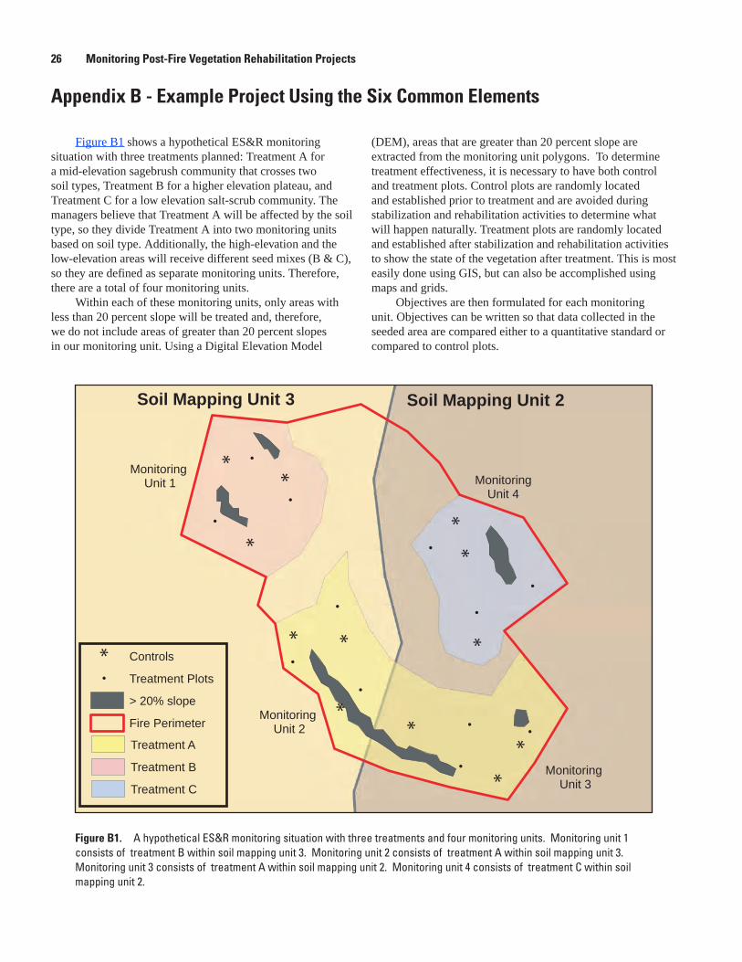
Figure B1 shows a hypothetical ES&R monitoring situation with three treatments planned: Treatment A for a mid-elevation sagebrush community that crosses two soil types, Treatment B for a higher elevation plateau, and Treatment C for a low elevation salt-scrub community. The managers believe that Treatment A will be affected by the soil type, so they divide Treatment A into two monitoring units based on soil type. Additionally, the high-elevation and the low-elevation areas will receive different seed mixes (B & C), so they are defined as separate monitoring units. Therefore, there are a total of four monitoring units.

Within each of these monitoring units, only areas with less than 20 percent slope will be treated and, therefore, we do not include areas of greater than 20 percent slopes in our monitoring unit. Using a Digital Elevation Model

(DEM), areas that are greater than 20 percent slope are extracted from the monitoring unit polygons. To determine treatment effectiveness, it is necessary to have both control and treatment plots. Control plots are randomly located and established prior to treatment and are avoided during stabilization and rehabilitation activities to determine what will happen naturally. Treatment plots are randomly located and established after stabilization and rehabilitation activities to show the state of the vegetation after treatment. This is most easily done using GIS, but can also be accomplished using maps and grids.

Objectives are then formulated for each monitoring unit. Objectives can be written so that data collected in the seeded area are compared either to a quantitative standard or compared to control plots.

Soil Mapping Unit 3 Soil Mapping Unit 2

Monitoring Unit 1

Monitoring Unit 2

Monitoring Unit 3

MonitoringUnit 4

Controls

Treatment Plots

> 20% slope

Fire Perimeter

Treatment A

Treatment B

Treatment C

Appendix B - Example Project Using the Six Common Elements

Figure B1. A hypothetical ES&R monitoring situation with three treatments and four monitoring units. Monitoring unit 1 consists of treatment B within soil mapping unit 3. Monitoring unit 2 consists of treatment A within soil mapping unit 3. Monitoring unit 3 consists of treatment A within soil mapping unit 2. Monitoring unit 4 consists of treatment C within soil mapping unit 2.


In the following examples, density is the attribute of primary interest. Plant density data were collected within each plot, and each plot consisted of three permanent 50-m transects established in accordance with the Monitoring Manual for Grassland, Shrubland, and Savanna Ecosystems. Along each transect, 1 x 1 m quadrats are placed at 10 locations. The numbers of perennial species are counted within each quadrat and averaged, resulting in an estimate of density (number of plants per square meter or hectare, by species or life form). The objective of the data collection is to determine if the average plant density of the treated areas is either clearly at or above an established target or the average of the controls. Below are general procedures for comparing treatment plots to a quantitative objective and comparing treatment plots to control plots. These procedures assume that the data are normally distributed.

Note that the objectives described below are written to reflect the minimum level acceptable to management. In our monitoring, we are seeking clear evidence that this minimum objective has been achieved. Writing objectives in this manner makes it easier to determine success.

Below we provide three procedures that may be used to test the effectiveness of treatments. After that, we provide detailed examples of developing and testing the effectiveness of treatments. A spreadsheet designed to help with these calculations can be downloaded at http://fresc.usgs.gov/research/esrmonitoring/Tools.htm

Procedure 1: Comparing treatment plots to a quantitative objective (graphical analysis)

This procedure uses a graphical approach to determine whether or not the quantitative objective of the ES&R treatment has been met. This is evaluated by comparing the means and confidence intervals of the data to the objective.

Management Objective: Attain an average density of perennial native seeded grasses in Monitoring Unit 1 of at least 2.5 plants/m2 by the end of the third growing season following treatment.

Sampling Objective: We want to be 90 percent certain that we have estimated the density of plants to within 20 percent of the true mean (α = 0 1. , d = 0.2).

1. Estimate the required sample size using equation B1 and estimate standard deviation from previous data or expert opinion. This equation requires you to estimate the precision (1/2 confidence limit) that you want to achieve. For the sampling objective above (20 percent), the precision will be 0.2* X . Additionally, you will enter the alpha level (α) and z-coefficient for your sample size. The results of the equation must be adjusted using the table in Elzinga et al. (1998) from Kupper and Hafner (1989). This adjustment can also be done automatically using the directions found in Elzinga et al. (1998), Appendix 16, page 447, and the computer program - PC Size: Consultant (Dallal, 1990).

nZ S

d=

( ) ( )( )

α2 2

2 , (B1)

where:


S is standard deviation of treatment data,

Zαis Z-coefficient for type I error rate (alpha level), and

d is desired level of precision in absolute terms (0.2* X ).

2. Collect data from a random sample of size n (determined in step 1) of all initial treatment plots.

3. Calculate sample statistics (mean, standard deviation, confidence interval). Confidence interval is calculated using this equation:

X Sn

t n±

( )−α( ),2 1

, (B2)

where:

X is the mean of the sample,

S is the sample standard deviation,

n is the number of samples collected, and

tα(2), n-1is the 2-sided t-value from a t-table for the appropriate alpha level and n-1 degrees of freedom.

4. Compare data collected using the specified confidence interval to the defined standard. Determine which of these four situations exist (fig. B2):

A. The sample mean and confidence interval (CI) fall below the objective. Conclude that the objective has not been met.

B. The sample mean is below the quantitative objective, but the upper limit of the confidence interval is above the objective. In this situation, it is possible that the objective has been met, but it is unlikely. Additional sampling could decrease the width of the confidence interval (precision), but is unlikely to move both the mean and the lower confidence limit above the objective. In these types of situations, it may be best to report the mean and confidence interval of the parameter being measured without additional sampling.

C. The sample mean is above the quantitative objective, but the lower limit of the confidence interval is below the objective. Additional sampling may move the mean or shrink the confidence interval to be completely above the quantitative objective. If additional sampling is not possible, then report the mean and confidence interval.

•

•

•

Appendix B - Example Project Using the Six Common Elements ��

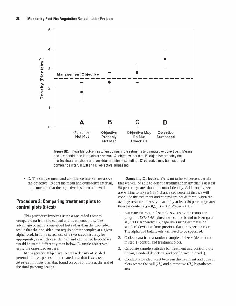
http://fresc.usgs.gov/research/esrmonitoring/Tools.htm

http://fresc.usgs.gov/research/esrmonitoring/Tools.htm

D. The sample mean and confidence interval are above the objective. Report the mean and confidence interval, and conclude that the objective has been achieved.

Procedure �: Comparing treatment plots to control plots (t-test)

This procedure involves using a one-sided t-test to compare data from the control and treatments plots. The advantage of using a one-sided test rather than the two-sided test is that the one-sided test requires fewer samples at a given alpha level. In some cases, use of a two-sided test may be appropriate, in which case the null and alternative hypotheses would be stated differently than below. Example objectives using the one-sided test are:

Management Objective: Attain a density of seeded perennial grass species in the treated area that is at least 50 percent higher than that found on control plots at the end of the third growing season.

• Sampling Objective: We want to be 90 percent certain that we will be able to detect a treatment density that is at least 50 percent greater than the control density. Additionally, we are willing to take a 1 in 5 chance (20 percent) that we will conclude the treatment and control are not different when the average treatment density is actually at least 50 percent greater than the control (α = 0 1. , β = 0.2, Power = 0.8).

1. Estimate the required sample size using the computer program DSTPLAN (directions can be found in Elzinga et al., 1998, Appendix 16, page 447) using estimates of standard deviation from previous data or expert opinion The alpha and beta levels will need to be specified.

2. Collect data from a random sample of size n (determined in step 1) control and treatment plots.

3. Calculate sample statistics for treatment and control plots (mean, standard deviation, and confidence intervals).

4. Conduct a 1-sided t-test between the treatment and control plots where the null (H

o) and alternative (H

a) hypotheses

are:

Figure B�. Possible outcomes when comparing treatments to quantitative objectives. Means and 1-α confidence intervals are shown. A) objective not met, B) objective probably not met (evaluate precision and consider additional sampling), C) objective may be met, check confidence interval (CI) and D) objective surpassed.


H X X

H X Xo t c

a t c

: .

: .

≤

>

1 5

1 5 , (B3)

where X is the mean of the sample (subscript t and c represent treatment and control plots).

In order to conduct the t-test, both the standard error and the degrees of freedom must be known. Formulas that adjust for unequal variances and sample sizes are used to ensure an accurate test.

Note: When success is defined in terms of controls, as is the case in procedure 2, it is necessary to adjust the values for the control plots in the equations for the t-test, standard error, and effective degrees of freedom. In the management objective for procedure 2, success is defined as when the density of perennial grasses in the treatment plots is at least 50 percent (1.5 times) higher than the density in the control plots. Therefore, the mean and standard deviation (S) of the control plots need to be multiplied by 1.5 in the equations for the t-test, standard error, and effective degrees of freedom. If success were defined as the cover of perennial grasses in the treatment plots being 100 percent (2 times) higher than the control plots, the mean and standard deviation of the control plots would need to be multiplied by 2.

The formula for the standard error is:

SESn

SnX X

t

t

c

ct c− = +1 5

2 2 21 5.

. , (B4)

where

SEX Xt c−1 5. is the standard error of the difference of two means, allowing unequal variances and sample sizes,

n is the number of samples collected (subscript t and c represent treatment and control plots), and

S is the sample standard deviation.

In cases where we have unequal variances, it is necessary to calculate the effective degrees of freedom using Satterthwaite’s approximation. Otherwise, degrees of freedom can be calculated as n

t + n

c -2.

Effective df =

S n S n

S n n

t t c

t t t

c2 2 2 2

2 2

1 5

1 1

/ /.

/ /( )+( )

( ) −

+ .. / /( )5 12 2 2S n nc c c( ) −

, (B5)

where:



The formula for the t-test is:

tX XSE

t c

X Xt c

=−

−

1 5

1 5

.

.

, (B6)

where:

t is the approximate test statistic,

X is the mean of the sample (subscript t and c represent treatment and control plots), and

SEX Xt c−1 5. is the standard error of the difference of two means, allowing unequal variances and sample sizes.

5. Compare the t-statistic to the critical value for t from a one-sided t-table with the appropriate alpha level and degrees of freedom.

6. If the test is significant, then reject Ho and conclude that

the average treatment density is at least 50 percent greater than Xc .

7. If the test is non-significant, there is no evidence that the treatment is greater than 1 5. Xc . Calculate and report the minimum detectable difference and power.

Procedure �: Comparing treatment plots to control plots (graphical analysis)

Some authors have advocated comparing two means by using a graphical analysis rather than a t-test (Di Stefano, 2004). Using this approach, a confidence interval for the difference between the two means is calculated. If the confidence interval contains 0, there is inadequate evidence that the two means are different. If the confidence interval does not contain 0, then the two means differ statistically, but they may not be ecologically significant. Therefore, you must define the difference between the two means that is ecologically important. Below we use the same objective as in Procedure 2.

Management Objective: Attain a density of perennial seeded grass species in the treated area that is at least 50 percent higher than that found on control plots at the end of the third growing season.

Sampling Objective: We want to be 90 percent certain that we will be able to detect a treatment density that is at least 50 percent greater than the control density. Additionally, we are willing to take a 1 in 5 chance (20 percent) that we will conclude the treatment and control are not different when the average treatment density is actually at least 50 percent greater than the control (α = 0 1. , β = 0.2, Power = 0.8).

1. Estimate the required sample size using the computer program DSTPLAN (directions can be found in Elzinga et al., 1998) using estimates of standard deviation from previous data or expert opinion. Also enter the alpha and beta level desired.

Appendix B - Example Project Using the Six Common Elements �9

2. Collect data at control and treatment plots.

3. Calculate sample statistics for treatment and control plots (mean, standard deviation, and confidence intervals).

4. Calculate the confidence interval for the difference between the two samples. In order to do this calculation, both the standard error and the degrees of freedom must be known. Formulas that adjust for unequal variances and sample sizes are used to ensure an accurate test.

Note: When success is defined in terms of controls, as is the case in procedure 2, it is necessary to adjust the values for the control plots in the equations for the t-test, standard error, and effective degrees of freedom. In the management objective for procedure 2, success is defined as when the density of perennial grasses in the treatment plots is at least 50 percent (1.5 times) higher than the density in the control plots. Therefore, the mean and standard deviation (S) of the control plots need to be multiplied by 1.5 in the equations for the t-test, standard error, and effective degrees of freedom. If success were defined as the cover of perennial grasses in the treatment plots being 100 percent (2 times) higher than the control plots, the mean and standard deviation of the control plots would need to be multiplied by 2.

The formula for standard error with unequal variances is:

SESn

SnX X

t

t

c

ct c− = +1 5

2 2 21 5.

. ,

where:

SEX Xt c−1 5. is the standard error of the difference of two means, allowing unequal variances and sample sizes,



In cases where we have unequal sample sizes, it is necessary to calculate the effective degrees of freedom using Satterthwaite’s approximation. Otherwise, degrees of freedom can be calculated as n

t + n

c -2.

Effective df =

S n S n

S n n

t t c

t t t

c2 2 2 2

2 2

1 5

1 1

/ /.

/ /( )+( )

( ) −

+ .. / /( )5 12 2 2S n nc c c( ) −

,

where:



The confidence interval of the difference is then calculated as:

X X S tt c X X dft c− ± ( )( )−1 5 2. ( ),α , (B7)

where:

X is the mean of the sample (subscript t and c represent treatment and control plots),

SEX Xt c−1 5.is the standard error of the difference of two means, allowing unequal variances and sample sizes, and

tα(2), df is the 2-sided t-value from a t-table for the appropriate alpha level and the effective degrees of freedom.

Determine which of the following cases exist (fig. B3):

A. The mean and confidence interval for the difference between the two means is completely above the level of ecological significance (5 plants/m2). Conclude that the difference between the two is ecologically significant (treatment was successful).

B. The difference of the mean between the treatment and control is above the level of ecological significance, but the lower confidence limit for the difference is below the level of ecological significance. Additional sampling may move the mean and confidence interval above the level of ecological significance. If additional sampling is not possible, report the mean and confidence interval.

C. The difference between the mean of the treatment and control is below the level of ecological significance, but the upper confidence limit for the difference is above the level of ecological significance. Additional sampling may move the mean and confidence interval above the level of ecological significance. However, this is unlikely. Report the mean and confidence interval.

D. The mean of the difference between the mean and confidence interval of the treatment and control is below the level of ecological significance. Conclude that there is no ecologically significant difference between the control and treatment plots.

E. The mean of the difference between the treatment and control plots is above zero, but the lower confidence limit is below 0 (no difference) and the upper confidence limit is above 5 plants/m2. Conclude that the data are not sufficient to arrive at a decision. However, it is unlikely that any difference is ecologically significant.

•

•

•

•

•


Figure B�. Data from the first five treatment plots of Example 1 where X = 3.5 plants/m2, S = 1.4 plants/m2 and n = 5. The mean is above the standard, but the lower limit of the confidence interval is below the standard.

F. The mean of the difference between the treatment and control plots is above 0, but the lower confidence limit is below 0 and the upper confidence limit is below the level of ecological significance. Conclude that there is no evidence to indicate that the treatment plots are ecologically different from the control plots. This conclusion also applies to any case where the mean of the difference falls below 0.

Example 1: Comparing treatment plots to a quantitative objective (graphical analysis)

Management Objective: Attain a density of perennial native seeded grasses in monitoring unit 1 of at least 2.5 plants/m2 by the end of the third growing season following treatment.

Sampling Objective: Obtain estimates of the mean number of plants/m2 with 90 percent confidence intervals that are within 20 percent of the true density (α = 0.1, d = 0.2).

The data from treatment plots will be compared to the quantitative management objective (2.5 plants/m2). The data from the first five treatment plots is shown in figure B4.

•

Figure B�. Possible outcomes when comparing treatments. Means and (1-α) percent confidence intervals of the difference are shown. The dashed line at 5 represents an ecologically significant difference between the treatment and control plots while the solid line represents no difference between the treatment and control plots (derived from DiStefano, 2004.)

Appendix B - Example Project Using the Six Common Elements �1

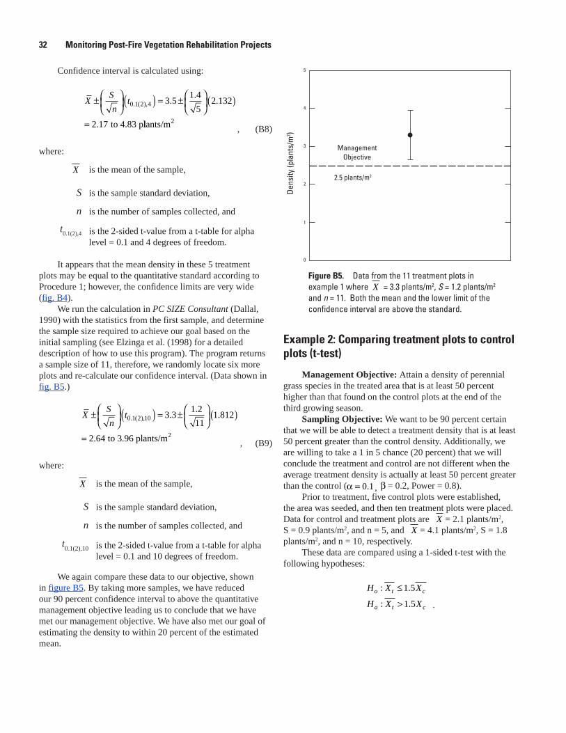
Confidence interval is calculated using:

X Sn

t±

( ) = ±

( )

=

0 1 2 4 3 5 1 45

2 132

2 17

. ( ), . . .

. to 4.83 pllants/m2, (B8)

where:




t0.1(2),4 is the 2-sided t-value from a t-table for alpha

level = 0.1 and 4 degrees of freedom.

It appears that the mean density in these 5 treatment plots may be equal to the quantitative standard according to Procedure 1; however, the confidence limits are very wide (fig. B4).

We run the calculation in PC SIZE Consultant (Dallal, 1990) with the statistics from the first sample, and determine the sample size required to achieve our goal based on the initial sampling (see Elzinga et al. (1998) for a detailed description of how to use this program). The program returns a sample size of 11, therefore, we randomly locate six more plots and re-calculate our confidence interval. (Data shown in fig. B5.)

X Sn

t±

( ) = ±

( )

=

0 1 2 10 3 3 1 211

1 812

2 64

. ( ), . . .

. to 3.96 plants/m2, (B9)

where:




t0.1(2),10 is the 2-sided t-value from a t-table for alpha

level = 0.1 and 10 degrees of freedom.

We again compare these data to our objective, shown in figure B5. By taking more samples, we have reduced our 90 percent confidence interval to above the quantitative management objective leading us to conclude that we have met our management objective. We have also met our goal of estimating the density to within 20 percent of the estimated mean.

Example �: Comparing treatment plots to control plots (t-test)

Management Objective: Attain a density of perennial grass species in the treated area that is at least 50 percent higher than that found on the control plots at the end of the third growing season.


Prior to treatment, five control plots were established, the area was seeded, and then ten treatment plots were placed. Data for control and treatment plots are X = 2.1 plants/m2, S = 0.9 plants/m2, and n = 5, and X = 4.1 plants/m2, S = 1.8 plants/m2, and n = 10, respectively.

These data are compared using a 1-sided t-test with the following hypotheses:

H X X

H X Xo t c

a t c

: .

: .

≤

>

1 5

1 5 .

Figure B�. Data from the 11 treatment plots in example 1 where X = 3.3 plants/m2, S = 1.2 plants/m2 and n = 11. Both the mean and the lower limit of the confidence interval are above the standard.


FRESC19-0087_fig05

ManagementObjective

2.5 plants/m2

Dens

ity (p

lant

s/m

2 )

5

4

3

2

1

0

Because there are unequal sample sizes with potentially unequal variances, we use the following standard error formula.

SESn

SnX X

t

t

c

ct c− = +

= + +

= −

=

1 5

2 2 2

2 2 2

1 5

1 810

1 5 0 95

0 324 0 3645

..

. . .

. .

00 830. plants/m2 , (B10)

where:

SEX Xt c−1 5. is standard error of the difference of two means, allowing unequal variances and sample sizes,

S is standard deviation, subscript c and t represent treatment and control plots, and

n is number of samples collected.

The effective degrees of freedom must also be calculated:

S n S n

S n n S n

t t c

t t t c c

c2 2 2 2

2 2 2 2 2

1 5

1 1 5

/ . /

/ . // /( ) (+( )

( ) −

+ ( ) nnc −

=

1

10 56 10

). ) ( , (B11)

where:

S is standard deviation, subscript c and t represent treatment and control plots, and

n is number of samples collected.

The formula for the t-test is:

tX XSE

t c

X Xt c

=−

= − =−

1 5 4 10 3 150 830

1 141 5

. . ..

..

, (B12)

where:

t is the approximate test statistic,

X is mean of control and treatment plots, and

SEX Xt c−1 5.is standard error of the difference of two means, allowing unequal variances and sample sizes.


We are looking for a treatment value of 150 percent of the control density (2.1*1.5 = 3.15 plants/m2). The critical value for the one-sided t-test with α = 0 1. and 10 degrees of freedom is 1.372. For the one-sided t-test, we need a value greater than 1.372 to reject the null hypothesis. The test statistic was 1.14, leaving us with inadequate evidence to conclude that density of the treatment plots is greater than or equal to 1.5 Xc .

We can calculate the power and minimum detectable change for the samples collected so far (procedure B from Elzinga et al., 1998, Appendix 16). Using DSTPLAN, we calculate that the power attained is 0.570, and the minimum detectable change (MDC) was 1.548. In this case, we wanted to be able to detect a difference of 50 percent above the control plots (2.1*0.5 = 1.05) with a power of 0.8. Therefore, we did not meet our goals for MDC or power, but it appears that additional sampling would increase the MDC and power and may result in a significant test.

These same equations can be used for other vegetation attributes. Different situations may occur in which different equations for sample size and t-tests may be required. The monitoring manuals reviewed in this paper, particularly Elzinga et al. (1998), discuss this in greater detail. Additional information and examples on statistical analysis can be found in Bonham (1989), Herrick et al. (2005b), and Zar (1999).

Example �: Comparing treatment plots to control plots (graphical analysis)

Management Objective: Attain a density of perennial grass species in the treated area that is greater than 50 percent higher than that found on the control plots at the end of the third growing season.


Prior to treatment, five control plots were randomly established, the area was seeded, and then ten treatment plots were randomly located. The data generated for the control and treatment plots in this example are as follows:

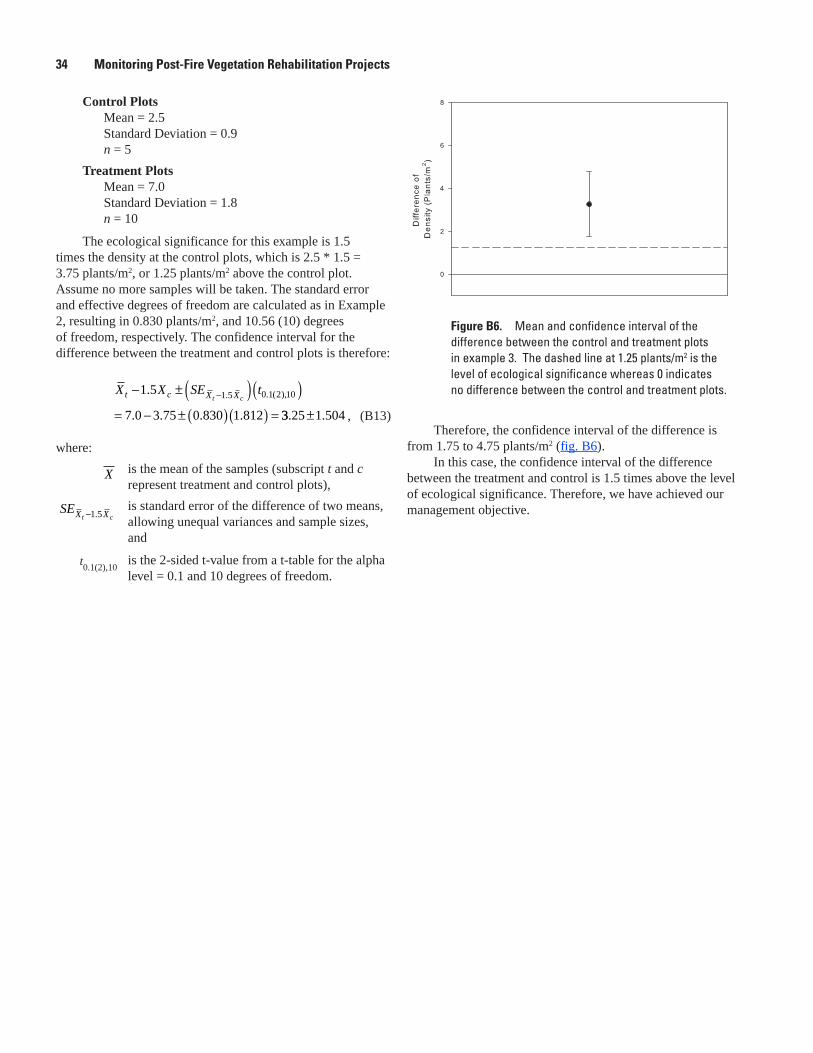
Control Plots Mean = 2.5 Standard Deviation = 0.9 n = 5

Treatment Plots Mean = 7.0 Standard Deviation = 1.8 n = 10

The ecological significance for this example is 1.5 times the density at the control plots, which is 2.5 * 1.5 = 3.75 plants/m2, or 1.25 plants/m2 above the control plot. Assume no more samples will be taken. The standard error and effective degrees of freedom are calculated as in Example 2, resulting in 0.830 plants/m2, and 10.56 (10) degrees of freedom, respectively. The confidence interval for the difference between the treatment and control plots is therefore:

X X SE tt c X Xt c− ± ( )( )

= − ± ( )( ) =−1 5

7 0 3 75 0 830 1 8121 5 0 1 2 10.

. . . .. . ( ),

33 25 1 504. .± , (B13)

where:

X is the mean of the samples (subscript t and c represent treatment and control plots),

SEX Xt c−1 5.is standard error of the difference of two means, allowing unequal variances and sample sizes, and

t0.1(2),10is the 2-sided t-value from a t-table for the alpha level = 0.1 and 10 degrees of freedom.

Figure B�. Mean and confidence interval of the difference between the control and treatment plots in example 3. The dashed line at 1.25 plants/m2 is the level of ecological significance whereas 0 indicates no difference between the control and treatment plots.


Therefore, the confidence interval of the difference is from 1.75 to 4.75 plants/m2 (fig. B6).

In this case, the confidence interval of the difference between the treatment and control is 1.5 times above the level of ecological significance. Therefore, we have achieved our management objective.


Additional Objectives

The following are additional examples of potential objectives related to ES&R treatments:

Silt Fences

Comparison to a standard Management Objective: Keep the amount of erosion on

the hillslopes in the native seedmix treatment below 1 ton/ha.Monitoring Objective: Obtain estimates of the erosion

(tons/ha) with 90 percent confidence intervals that are within 20 percent of the estimated value.

Comparison between control and treatment plotsManagement Objective: Reduce the amount of erosion

on hillslopes in the native seedmix treatment as compared to the control areas during the first year post-fire.

Monitoring Objective: We want to be 90 percent certain that the erosion (kg/ha) in the treatment plots is lower than in the control plots. Additionally, we are willing to take a 1 in 5 chance (20 percent) that we will conclude that the amount of erosion in the treatment plots is equal to or greater than the erosion in the control plots when the average erosion in the treatment plots is less than the erosion in the control plots (α = 0 1. , β = 0.2, Power = 0.8).

Exotic Species

Comparisons to a standardManagement Objective: Reduce the cover of exotic

annual grass species to less than 25 percent in the native seedmix treatment area.

Monitoring Objective: Obtain estimates of the cover of exotic annual grass species with 90 percent confidence intervals that are within 20 percent of the estimated value (α = 0 1. , d = 0.2).

Comparison between control and treatment plotsManagement Objective: Reduce the cover of exotic

annual grasses (Bromus tectorum, Taeniatherum caput-medusae) to significantly less than control plots in the native seeding treatment.

Monitoring Objective: We want to be 90 percent certain that the cover (percent) of exotic annual grasses in the treatment plots is less than in the control plots. Additionally, we are willing to take a 1 in 5 chance (20 percent) that we will conclude that the cover of exotic annual grasses in the treatment plots is equal to or greater than the cover of exotic annual grasses in the control plots when the cover in the treatment plots is less than in the control plots (α = 0 1. , β = 0.2, Power = 0.8).

Additional examples can be found in Elzinga et al. (1998) and USDI National Park Service (2003).

This page is intentionally left blank.


Monitoring Post-Fire Vegetation Rehabilitation Projects: A Com

mon A

pproach for Non-Forested Ecosystem

s

Printed on Recycled Paper

Wirth and Pyke

SIR 2006–5048

monitoring post-fire vegetation rehabilitation projects: a common

Documents