monitoring programmable logic controllers - autenticação · thesis to obtain the master of...
TRANSCRIPT

Monitoring Programmable Logic Controllers
Henrique de Almeida Gonçalves
Thesis to obtain the Master of Science Degree in
Electrical and Computer Engineering
Supervisor: Professor José António da Cruz Pinto Gaspar
Examination Committee
Chairperson: Professor João Fernando Cardoso Silva Sequeira
Supervisor: Professor José António da Cruz Pinto Gaspar
Member of the Committee: Professor Paulo Jorge Coelho Ramalho Oliveira
November 2015


Agradecimentos
Gostaria de agradecer ao meu orientador Professor José António Gaspar toda a disponibilidade
e apoio prestados no decorrer desta dissertação. Agradeço também ao Ricardo Nunes a disponi-
bilidade e ajuda que deu.
Quero agradecer aos meus pais por me terem possibilitado a realização do Mestrado em
Engenharia Electrotécnica e de Computadores e pelo apoio incondicional que sempre me deram.
Agradeço também o apoio da minha restante família e amigos. Atodos eles um muito obrigado.

ii

Resumo
Os Sistemas de Eventos Discretos (DES) estão omnipresentesem aplicações industriais. Os
Controladores Lógicos Programáveis (PLC) são os dispositivos normalmente utilizados para
implementar DES em ambiente industrial. O desenho de um DES ea implementação em PLC
é um processo moroso que requer tipicamente múltiplas verificações e uma validação final.
A nossa abordagem de desenho de um DES envolve a utilização deredes de Petri (PN).
Como forma de agilizar a implementação do DES propomos converter automaticamente a PN
em código Structured Text (ST), i.e. uma linguagem standardde programação de PLCs. Desen-
volvemos um sistema de monitorização de PLC com o objectivo de verificar que um programa
PLC cumpre os requisitos desejados.
Neste relatório detalhamos a construção de hardware de monitorização de inputs e outputs
de um PLC. O custo do hardware é mantido baixo pela utilização de uma placa de microcon-
trolador Arduino Mega. Detalhamos também o desenvolvimento de hardware adicional para
interconectar o monitor ao PLC e a um processo que desejamos controlar.
O hardware desenvolvido e o DES implementado permitem observar o funcionamento do
PLC, por exemplo a variabilidade do tempo de um Scan Cycle, e validar a implementação de
um caso de estudo, nomeadamente um DES associado à leitura deum teclado.
Palavras chave:Monitor de Sinais, Sistemas de Eventos Discretos, Controlador Lógico Pro-
gramável, Arduino, Rede de Petri, Structured Text.

iv

Abstract
Discrete Event Systems (DES) are ubiquitous in industrial applications. Programmable Logic
Controllers (PLC) are commonly used to implement DES. Designing a DES and implementing
in a PLC is a lengthy process typically requiring multiple verifications and an end process
validation.
Our approach to design a DES involves using Petri Nets (PN). Then we propose an automatic
conversion of the PN to Structured Text (ST) code, a standardPLC programming language.
With the objective of verifying that the PLC program fulfillsdesign specifications we develop a
PLC monitoring system.
Construction of a hardware PLC Signal Acquirer, able to monitor PLC inputs and outputs,
is detailed in this work. Cost is kept low by using the affordable microcontroller board Arduino
Mega. Development of additional hardware is also detailed,having the purpose of intercon-
necting the monitor with the PLC and the controlled plant.
With our hardware developed and DES implemented we show characteristics of the PLC
behavior, as the variability of the scan cycle time, and validate the DES implementation of a
keyboard reading case study.
Keywords: Signal Acquirer, Discrete Event Systems, Programmable Logic Controllers, Ar-
duino, Petri Net, Structured Text.

vi

Contents
Agradecimentos i
Resumo iii
Abstract v
1 Introduction 1
1.1 Related Work . . . . . . . . . . . . . . . . . . . . . . . . . . . . . . . . . . . 2
1.2 Objectives and Challenges . . . . . . . . . . . . . . . . . . . . . . . . . .. . 4
1.3 Thesis Structure . . . . . . . . . . . . . . . . . . . . . . . . . . . . . . . . .. 4
2 Discrete Event Systems 7
2.1 Petri Net Language . . . . . . . . . . . . . . . . . . . . . . . . . . . . . . . .7
2.1.1 Definition . . . . . . . . . . . . . . . . . . . . . . . . . . . . . . . . . 8
2.1.2 Transition . . . . . . . . . . . . . . . . . . . . . . . . . . . . . . . . . 9
2.1.3 Incidence Matrix . . . . . . . . . . . . . . . . . . . . . . . . . . . . . 9
2.2 Properties . . . . . . . . . . . . . . . . . . . . . . . . . . . . . . . . . . . . . 10
2.2.1 Supervision based on Linear Constraints . . . . . . . . . . . .. . . . . 11
2.2.2 Generalized Linear Constraints . . . . . . . . . . . . . . . . . . .. . . 12
3 PLC Data Acquisition 19
3.1 Hardware Setup . . . . . . . . . . . . . . . . . . . . . . . . . . . . . . . . . . 19
3.2 PLC Input and Output Connections . . . . . . . . . . . . . . . . . . . . .. . . 21
3.3 PLC Input and Output Monitor . . . . . . . . . . . . . . . . . . . . . . . .. . 22
3.4 Data Acquisition Software . . . . . . . . . . . . . . . . . . . . . . . . .. . . 26
3.4.1 Arduino Monitoring Program . . . . . . . . . . . . . . . . . . . . . .26
3.4.2 PC Monitoring Program . . . . . . . . . . . . . . . . . . . . . . . . . 27

viii CONTENTS
4 PLC Program Development and Monitoring 29
4.1 DES Implementation . . . . . . . . . . . . . . . . . . . . . . . . . . . . . . .29
4.2 Petri net Simulation . . . . . . . . . . . . . . . . . . . . . . . . . . . . . .. . 30
4.3 Petri net to PLC Conversion . . . . . . . . . . . . . . . . . . . . . . . . . .. 31
4.3.1 Petri net to Structured Text Compiler . . . . . . . . . . . . . . .. . . 31
5 Case study: Keyboard Reading 35
5.1 Proposed Petri Net Model . . . . . . . . . . . . . . . . . . . . . . . . . . .. . 36
5.2 Properties . . . . . . . . . . . . . . . . . . . . . . . . . . . . . . . . . . . . . 39
5.3 Supervisor . . . . . . . . . . . . . . . . . . . . . . . . . . . . . . . . . . . . . 41
5.4 Implementation . . . . . . . . . . . . . . . . . . . . . . . . . . . . . . . . . .47
6 Experiments 49
6.1 PLC Characterization . . . . . . . . . . . . . . . . . . . . . . . . . . . . . .. 49
6.2 Key detection . . . . . . . . . . . . . . . . . . . . . . . . . . . . . . . . . . . 55
6.3 Initial Marking Effect . . . . . . . . . . . . . . . . . . . . . . . . . . . .. . . 56
6.4 Supervisory Control . . . . . . . . . . . . . . . . . . . . . . . . . . . . . . .. 59
7 Conclusion and Future Work 65
A Arduino Shield for IO Monitoring 67
B PN to PLC Compiler Usage 71
C PLC Program 75
D Arduino program 85

List of Figures
2.1 Example of a Petri net . . . . . . . . . . . . . . . . . . . . . . . . . . . . . .. 9
2.2 Example of a Petri net . . . . . . . . . . . . . . . . . . . . . . . . . . . . . .. 10
2.3 Example of a reachability tree and its Petri net . . . . . . . .. . . . . . . . . . 11
2.4 Consumer-Producer situation with underflow buffer . . . . .. . . . . . . . . . 14
2.5 Petri net for a producer-consumer type situation . . . . . .. . . . . . . . . . . 14
2.6 Petri net with consumer-producer supervisor . . . . . . . . .. . . . . . . . . . 16
2.7 Consumer-Producer situation with underflow and overflow buffer . . . . . . . . 16
2.8 Petri net for a producer-consumer system . . . . . . . . . . . . .. . . . . . . 17
3.1 Generic setup block diagram. . . . . . . . . . . . . . . . . . . . . . . .. . . . 20
3.2 24 volt DC power supply (a). Modicon PLC (b). Terminal with twelve key
numbered keyboard (c). . . . . . . . . . . . . . . . . . . . . . . . . . . . . . . 20
3.3 Printed circuit board prototype designed for keyboard terminal, front (b), back
(d). Printed circuit board prototype designed for monitoring alternative PLC,
front (a), back (c). Assembled printed circuit boards, for PLC (e), and for ter-
minal (f). . . . . . . . . . . . . . . . . . . . . . . . . . . . . . . . . . . . . . 21
3.4 PLC to terminal connections using final PCBs manufactured at Eurocircuits [6]. 22
3.5 Arduino based pass through logic observer and referencegenerator . . . . . . . 23
3.6 Arduino Mega, part of the signal monitor (a). Designed Arduino Mega shield
PCB (b). Assembled signal monitor shield for Arduino Mega (c). Signal moni-
tor composed by Arduino Mega and Arduino shield (d). . . . . . . .. . . . . . 25
3.7 Generic setup with signal monitor assembled. . . . . . . . . .. . . . . . . . . 26
3.8 Simplified code for Matlab serial communication with Arduino. . . . . . . . . 28
5.1 Plc and terminal. . . . . . . . . . . . . . . . . . . . . . . . . . . . . . . . . .35
5.2 Incidence Matrix . . . . . . . . . . . . . . . . . . . . . . . . . . . . . . . . .37

x LIST OF FIGURES
5.3 Table with pre and post conditions for Petri net evolution (a). Developed Petri
net (b). . . . . . . . . . . . . . . . . . . . . . . . . . . . . . . . . . . . . . . 38
5.4 Petri net column scanning evolution. . . . . . . . . . . . . . . . .. . . . . . . 39
5.5 Petri net one key pressed evolution. . . . . . . . . . . . . . . . . .. . . . . . 39
5.6 Reachability Tree . . . . . . . . . . . . . . . . . . . . . . . . . . . . . . . . .41
5.7 Flag Petri net. . . . . . . . . . . . . . . . . . . . . . . . . . . . . . . . . . . 42
5.8 Flag Petri net method of operation. . . . . . . . . . . . . . . . . . . . . . . . 42
5.9 Flag Petri net incidence matrix. . . . . . . . . . . . . . . . . . . . . . . . . . 42
5.10 Supervised system incidence matrix. . . . . . . . . . . . . . . .. . . . . . . . 45
5.11 Petri net developed for keyboard control, with supervisor. . . . . . . . . . . . . 46
6.1 Experimental setup for PLC characterization (a). Closeup view of developed
monitor (b). Closeup view of developed monitor (c). Signal flow diagram for
the first experiment (d). PLC square wave generation program(e). . . . . . . . 50
6.2 PLC output captured by the Arduino based monitor, multiple experiments, 5
scan cycles window, first rising edge in each window shifted to t = 0 (a). All
rising edges shifted tot = 0 (b). Observed scan cycle times along 8 seconds
(c). Histogram of observed scan cycle times (d). . . . . . . . . . .. . . . . . . 51
6.3 Observing the time from a signal input (rising edge%i0.3.0) to a signal out-
put (rising edge%q0.3.16). PLC input delay test code. (a). Connections
diagram (b). Observed PLC input to output delays along 8 seconds (c) and
histogram of the delays (d). . . . . . . . . . . . . . . . . . . . . . . . . . . .. 52
6.4 Observing the time for 100ms period square signal detection. Connections dia-
gram (a). Observed PLC time of signal detection along 8 seconds (b). . . . . . 53
6.5 Varying scan cycle time. Minimum scan cycle time observed experimentally
(a). Maximum scan cycle time observed experimentally (b). .. . . . . . . . . 54
6.6 Setup used for experiments. Setup for monitoring PLC (a). Keyboard terminal
(b). . . . . . . . . . . . . . . . . . . . . . . . . . . . . . . . . . . . . . . . . . 55
6.7 PLC output captured by the Arduino based monitor, input data key sequence
(a). Input data, sequence of keys (b). Expected output, MatLab Simulation (c).
PLC output observed with the developed monitor (d). . . . . . . .. . . . . . . 56
6.8 PLC output captured by the Arduino based monitor, input data key sequence
(a). Initial marking of Petri net (b). Expected output, MatLab Simulation (c).
PLC output observed with the developed monitor (d). . . . . . . .. . . . . . . 57

LIST OF FIGURES xi
6.9 PLC output captured by the Arduino based monitor, initial marking of Petri net
(a). Expected output, MatLab Simulation (b). PLC output observed with the
developed monitor (c). . . . . . . . . . . . . . . . . . . . . . . . . . . . . . . 58
6.10 PLC output captured by the Arduino based monitor, initial marking of Petri net
(a). Expected output, MatLab Simulation (b). PLC output observed with the
developed monitor (c). . . . . . . . . . . . . . . . . . . . . . . . . . . . . . . 59
6.11 PLC output captured by the Arduino based monitor, inputdata key sequence
(a). Input data, sequence of keys (b). Expected output, MatLab Simulation (c).
PLC output observed with the developed monitor (d). . . . . . . .. . . . . . . 60
6.12 PLC output captured by the Arduino based monitor, multiple experiments, in-
put data key sequence (a). Input data, sequence of keys (b). Expected output,
MatLab Simulation (c). PLC output observed with the developed monitor (d). . 62
A.1 Arduino shield electronic schematic. . . . . . . . . . . . . . . .. . . . . . . . 68
A.2 Arduino shield PCB schematic. . . . . . . . . . . . . . . . . . . . . . . .. . . 69
A.3 Arduino shield physical PCB, front. . . . . . . . . . . . . . . . . . . .. . . . 69
A.4 Arduino shield physical PCB, back. . . . . . . . . . . . . . . . . . . . .. . . 70
B.1 Create a PLC program from a Petri Net and IO mapping. . . . . . . .. . . . . 72
B.2 Load a Petri Net from file. . . . . . . . . . . . . . . . . . . . . . . . . . . . .72
B.3 Define the mapping of PLC inputs to PN transitions. . . . . . . .. . . . . . . 73
B.4 Define the mapping of PN places to PLC outputs. . . . . . . . . . . .. . . . . 73

xii LIST OF FIGURES

List of Tables
4.1 plc_map_inputs ST compiler function description. . . . . . . . . . . . . . 32
4.2 plc_timed_transitions ST compiler function description. . . . . . . . 32
4.3 plc_encode_petri_net ST compiler function description. . . . . . . . . 33
4.4 plc_output_if_any_place ST compiler function description. . . . . . . 34
4.5 plc_encode_places ST compiler function description. . . . . . . . . . . . 34
5.1 DES events. . . . . . . . . . . . . . . . . . . . . . . . . . . . . . . . . . . . . 36
5.2 DES conditions. . . . . . . . . . . . . . . . . . . . . . . . . . . . . . . . . . .37

xiv LIST OF TABLES

Chapter 1
Introduction
Major automation companies offer modular digital computers that allow using a large variety,
and number, of electrical input and/or output interfaces, the so called Programmable Logic
Controllers (the term, and its abbreviation PLC, are registered trademarks of the Allen-Bradley
Company, although nowadays they are widely used as a generic description1 ). Together with
the hardware, the automation companies also offer, or sell,monitoring software. The software
interfaces are however usually closed. Whenever one wants todebug a PLC program, develop-
ing fast monitors of the physical inputs and outputs of a PLC is normally challenging or even
impossible with the tools provided by default by the automation companies.
A PLC cyclically performs (i) signals input reading, (ii) program execution, and (iii) signal
output writing. This is comparable to the definition of a Discrete Event System (DES), in which
the event of receiving a digital input generates digital output.
In this work we propose a methodology for developing and debugging PLC programs based
in formalized Discrete Event Systems (DES). DES are systemswith dynamics driven by event
occurrences, at possibly unknown irregular intervals, of physical events. Such systems are used
in a variety of contexts, from computer operating systems tothe control of complex processes.
Each event occurs at a particular instant in time and marks a change of state in the system.
Petri nets (PNs) are one of the most suitable and used forms ofmathematical representation
of event driven systems (DESs, PLC programs handling digital I/O). A Petri net can usually
be designed by analyzing the structure and dynamic behaviorof a system to be modeled. This
information is essential to implement DESs with stability and robustness specifications.
In order to minimize the usually lengthy process of design toimplementation, we propose
converting automatically PN to Structured Text (ST), a standard programming language of a
1http://www.machine-information-systems.com/PLC.html

2 Introduction
PLC. The necessary design verifications and final validation are helped by an external hardware
device inserted between the PLC and the plant to control, monitoring the inputs and outputs of
the PLC.
1.1 Related Work
Petri net theory was continually developed since its beginnings with Dr. Petri’s 1962 Ph.D.
Dissertation[22]. But it was not until 1981, that Peterson [21] wrote the book that presented all
the development work scattered among many sources in a coherent and consistent manner.
In 1967 Naylor and Finger [18], proposed a multistage process of validation. This validation
method consists of (1) developing the model on theory, observations, and general knowledge;
(2) validating the model assumptions where possible by empirically testing them; and (3) com-
paring (testing) the input-output relationships of the model to the real system.
In 1979 Schlesinger [25], defined Model validation to mean substantiation that a computer-
ized model within its domain of applicability possesses a satisfactory range of accuracy consis-
tent with the intended application of the model.
In 1992 [3], Cutts and Rattigan addressed the fact that most PLCprogrammers develop
programs using Ladder Logic, that makes a situation with a very large number of logical inputs
and logical combinations, very hard to control. In particular, in these systems are very hard to
predict the results of illegal inputs such as damaged input switches or sensors, causing stable
systems to be unpredictable and the control plant to have an unwanted behavior due to jumped
sequences, deadlock and lost components. As a solution to this problem, Cutts and Rattigan [3],
proposed to use software based on Petri nets for as a practical approach to modeling systems
before being implemented on PLCs.
In 1996 Roussel and Lesage state [23] : "‘The verification is theproof that the internal se-
mantics of a model is correct, independently from the modeled system. The searched properties
of the models are stability, deadlock existence, ... The validation determines if the model agrees
with the designer’s purpose."’
In 2002, Mertke and Frey [15], proposed a verification of PLC programs based on Petri nets.
Minas and Frey in 2002 [16], presented a graphical programming approach for PLCs based on
Petri nets. From their research and experience, they concluded that there was a need for a
PLC programing language that, "is capable of graphically describing sequential and concurrent
algorithms, gives visual feedback of the control-flow in these algorithm (current state, following
state etc.),is easy to apply, and is easy to implement i.e. results in fast code." To implement this

1.1 Related Work 3
approach they have usedDiagen, an environment capable of developing diagrams based in
a formal specification of the diagram language. The created Petri nets can then be translated
to equivalent PLC programing language Instruction List (IL). In [24] Klein, Frey and Minas,
described a methodology used by their software to generatedIL code from a Petri net. First a
Boolean variable is declared for each place of the Petri net, its value depends on the presence
of a token in the place. For the transitions, they are tested for firing and for being enabled,
returning 1 if all conditions are fulfilled. If a place is marked then the corresponding output
function is executed, if not a conditional jump to the next place is performed. In [24] there
is reference to implementation of a process to visualize themachine state within the Petri net
editor while the machine is running. Making the editor able to find out failures or deadlocks.
In 2004 conformance test, testing a PLC system seen as a black-box (its internal structure
is unknown) with observable inputs/outputs, is advocated by certification bodies and standards
[8].
In 2005 [2], develops method for the automatic generation oftest scenarios from the behav-
ioral requirements of a DES, that generates a suite of test scenarios applicable for black box
testing.
In 2011 Sargent [14], made a study of the several validation techniques and tests commonly
used in model validation, and purposed a model for several steps for validation of simulation
models, in which it is necessary to make comparisons betweenthe simulation model and system
behavior data for at least a few sets of experimental conditions, and preferably for several sets.
In 2013, Pereira and Gomes [20], developed an Automatic Petri net to VHDL software2,
that can also be used to transform Petri nets into other typesof programming languages.
Also 2013 Vargas, Mellado and Lesage [5] [4], developed a software tool for building auto-
matically interpreted Petri net models from an observed system input/output sequence.
Moody and Antsaklis [17] wrote the book in the subject of supervisory theory of DES using
Petri nets, and later Iordache, Antsaklis and Marian [10, 11, 12], and then Iordache, Antsaklis,
Marian and Panos [9, 13] published many works on further development of the subject of su-
pervisory control. Most of the work done by Antsaklis was developed in the context of the ISIS
group3, in which he is the director.
2http://gres.uninova.pt/3http://www3.nd.edu/~isis/index.html

4 Introduction
1.2 Objectives and Challenges
Programmable logic controllers (PLCs) are the main integration equipment used in automation
today. The most commonly used PLC programming language is ladder diagram. The anima-
tion of the ladder diagram is usually the only form of code validation. Automation companies
available monitoring software is usually closed, making the development of fast monitors of the
physical inputs and outputs of a PLC, challenging or even impossible with the tools provided.
In this thesis we develop PLC monitoring with the objective of verifying that a PLC pro-
gram fulfills the design specifications. In other words, we want a design validation procedure
applicable to a discrete event system (DES) implemented in aPLC. We assume that the input
and output events during a finite amount of time are enough to characterize the DES. Hence, our
validation procedure will be based in observing input and output signals (events) of the DES.
Our approach for building and debugging a DES implemented with a PLC is the following:
(i) Design one PN solving the same problem that the DES will solve. In this step we avoid
some problems by design, e.g. not using unobservable transitions, preventing deadlocks, etc.
(ii) Simulating the PN and saving input and output signals. (iii) Encode the PN into a PLC
language. (iv) Compare simulation with real run.
Observing input and output events can be done to some extent using the PLC memory.
This is however limited by the free memory available in the PCLafter implementing the DES.
Alternatively, we propose logging input and output signalsusing external hardware, with a
sampling time shorter than the PLC scan cycle.
There are many publications focusing on process modeling, analysis and validation [3, 15,
16, 24, 26]. The common approach is modeling the system with aPetri net, and then generating
the ladder diagram from it. Petri nets deliver correct and dependable PLC programs.
In this work is proposed the construction of an hardware PLC Signal Acquirer, able to
monitor analyze and validate PLC programs. A hardware interface has the advantage of a much
higher operating frequency compared to a monitoring software. In addition, being an external
hardware interface, one has the guarantee that monitoring does not increase the memory/time
complexity of the PLC software.
1.3 Thesis Structure
Chapter 1 identifies the problem to approach in the thesis and proposes a path with theoretical
support. It also presents a short discussion on the state of the art of Petri nets and its application
in PLCs. Chapter 2 presents a theoretical introduction to Petri nets, its properties and methods

1.3 Thesis Structure 5
of analysis. Chapter 3 presents developed hardware for PLC monitoring. Chapter 4 presents
an approach to hardware PLC program development and monitoring based in Petri net theory.
Chapter 5 provides a theoretical analysis of our case study, base on Petri net theory and using
supervision control. Chapter 5 presents the experiments andrespective results obtained. Chap-
ter 6 summarizes the work performed, its achievements, and proposes further work to extend
the activities described in this document.

6 Introduction

Chapter 2
Discrete Event Systems
In this chapter we introduce Discrete Event Systems (DES). The structure of the introduction
is based in the course Industrial Processes Automation by Professor Paulo Oliveira [19]1 and in
books [21, 17, 1].
A DES can be characterized by a discrete state space whose state transitions happen at dis-
crete points in time due to events [1]. More in detail, the DESevolution, or state transition, is
a result of combining asynchronous and concurrent event processes. An event occurs instan-
taneously and causes transitions from one discrete state toanother. An event can be a specific
action taken (e.g. button pressed), a spontaneous occurrence dictated by nature (hardware fail-
ures), a sudden fulfillment of some conditions (e.g. buffer full).
DESs are usually implemented using Programmable Logic Controllers (PLCs). In generic
terms one PLC is composed of tree major parts, namely inputs,outputs and a control processor.
When an input changes, the control processor responds by changing an output. This can be
compared to the the state change that leads to an event occurrence in a DES.
2.1 Petri Net Language
Petri nets allow representing general DES, whose operationdepends on potentially complex
control schemes. In Petri nets, events change in accordanceto a set of rules. Graphically repre-
sentation of Petri nets, result in Petri net graphs that are intuitive and capture a lot of structural
information about the system. Analysis techniques have been developed for the studying of
Petri nets. These techniques include reachability analysis, well as linear-algebraic techniques.
Petri nets as representations of Discrete Event Systems have high degree of generality,
1https://fenix.tecnico.ulisboa.pt/disciplinas/APInd/2010-2011/1-semestre

8 Discrete Event Systems
specially when compared with used PLC programming languages, GRAFCET and Sequential
Function Chart (SFC). SFC and GRAFCET are both inspired from Petri nets and have compa-
rable structures. A live, safe, and reversible Petri net which has mutually exclusive transitions
can be implemented directly in SFC and GRAFCET.
A Petri net is represented graphically by:
• Transitions, events that can or not happen, graphically represented by bars.
• Places, conditions represented by circles.
• Oriented Arcs joining the circles and bars, conditions thatlead to events.
An arc can only connect transitions to places and vice-verse, there are no arcs connecting transi-
tions to transitions or places to places. Each place is associated with a natural number of marks.
The initial state representation, evolves according to a labeling transition function. The formal
definition of a Petri net is done in the next section.
2.1.1 Definition
A Petri net is a quintuplet, defined by parameters the parameters(P, T,A,W, x), where:
P = {p1, p2, ...pn}, n ≥ 0 P is a finite set of places;
(2.1)
T = {t1, t2, ...tm}, m ≥ 0 T is a finite set of transitions;
(2.2)
A ⊆ (P × T ) ∪ (T × P ) arcs that connect places to transitions and transitions to places;
(2.3)
W : A → {1, 2, 3, ...} is the weight function of the arches;
(2.4)
x = [x(p1), x(p2), ..., x(pn)] ∈ Nn represents the marking of places.
(2.5)
In describing Petri nets, places that are connected to the input of the transitiontj are represented
by I(tj). O(tj) represents places that are connected to the output of the transitiontj, i.e.:
I(tj) = {pi ∈ P : (pi, tj) ∈ A} (2.6)

2.1 Petri Net Language 9
O(tj) = {pi ∈ P : (tj, pi) ∈ A} (2.7)
In function (2.8),µ(k) represents the present marking,µ(k + 1) is the marking we want to
achieve,q(k) represents the triggering vector needed to go from the markingµ(k) to µ(k + 1)
andD is the incidence matrix that accounts the balance of tokens (giving the transitions fired).
The state evolution of a Petri net can be described as the following matrix function,
µ(k + 1) = µ(k) +D ∗ q(k) (2.8)
Figure 2.1 shows an exemple of a Petri net.
Figure 2.1: Example of a Petri net
2.1.2 Transition
The transitiontj ∈ T is active ifx(pi) ≥ w(pi, tj) for all pi ∈ I(tj). That is,tj transition is
enabled when the number of marks onpi is at least as great as the weight arc connectingpi to
tj for all pathspi that are inputs to the transitiontj.
The implementation of a transitiont is accomplished by removing each place of assembly
L, I(L, t) marks. After this,O(P, t) marks are set in each place of assembly P.
2.1.3 Incidence Matrix
DefiningD as the incidence matrix of a Petri net, a matrixm × n whose entry(j, i) comes in
the form,
Dji = w(tj, pi)− w(pi, tj) (2.9)

10 Discrete Event Systems
We can write the state equation,
x′ = X + µD. (2.10)
This equation describes the state transition process, as a result of inputµ . Considering the Petri
Figure 2.2: Example of a Petri net
net in Figure 2.2, we obtain the following incidence matrix,
D =
−1 1 1 0
0 0 −1 1
−1 0 −1 −1
(2.11)
2.2 Properties
In this chapter we describe Petri net properties. These properties provide us a way to character-
ize study systems.
Property 1. Reachability, a configuration of the marks over places M (marking), given aPetri
netN , is reachable ifM ∈ R(N), whereR(N) is the group of all the possible markings of N.
Property 2. Boundness, it is the property that verifies if the number of marks for allthe places
is limited. A place in a Petri net isk−bounded if it does not contain more thank marks in all
reachable markings.
Property 3. Safeness, a Petri net is safe if for every possible marking, there isn’t more then one
mark for each place. A Safe Petri net is 1-bounded.
Property 4. Conservation. A Petri net is strictly conservative, when for every markingthe total
number of marks remains the same. A Petri net is strictly conservative if for everyµ ∈ R(C, µ):
∑
pi∈P
µ′(pi) =∑
pi∈P
µ(pi)

2.2 Properties 11
Property 5. Liveness. This property is associated, with the possibility that a Petri net has of
running continuously without reaching a deadlock. A Petri net is alive if for all the possible
markings, there’s a trigger for another marking.
Property 6. Coverability. Given a Petri net with initial markingu0, the stateu′ ∈ R(C, u) is
covered ifu′(i) ≤ u(i), for all placespi ∈ P .
The set of all markings reachable from the initial stateu is the is called reachable set. The
graphic representation of a PN’s reachable set is called a reachability tree. An exemple of a
reachability tree and its PN is showned in Figure 2.3.
Figure 2.3: Example of a reachability tree and its Petri net
In a particular Petri netN , with initial statex0 , the statey coversx0 if there is ax ∈ R(N)
wherex(pi) ≥ y(pi) for all i = 1, ..., n.
In a give Petri netC = (P, T, I, O, u0), a placepi ∈ P is k-bounded ifu′
i ≥ k for u′ =
(u′
1, ..., u′
i, ..., uN′) ∈ R(C, u0)
If the Petri net of interest is bounded, then safety and blocking properties can be determined
algorithmically. A placepi ∈ P of the Petri netC = (P, T, I, O, u0) is safe if for allu′ ∈
R(C, u0) : ui′ ≥ 1 A Petri net is safe if all its places are safe.
Petri net N with initial statex0 is said to be live if there always exists some sample path such
that any transition can eventually fire from any state reached fromx0.
2.2.1 Supervision based on Linear Constraints
The goal of this chapter is to introduce the supervision of Petri nets. A supervisor is a discrete
event system that is used to monitor and control another discrete event system, satisfying a
specification. In a Petri net, a supervisor restricts transitions that may trigger at a given state of
the Petri net, so that the specification is satisfied. The specification may consist of requirements

12 Discrete Event Systems
concerning the reachable markings or permissible triggering sequences. The main supervision
approach referred is the supervision based on place invariants. We desire a supervisor to prevent
the system from reaching markings which do not satisfy,
Lµp ≤ b (2.12)
WhereL is an integernc × n matrix (nc is the number of constraints, n is the number of places
of the given Petri net),b is an integer column vector, andµ is the Petri net marking.
µc is a vector ofnc non-negative slack variables, defined as,
µc = b− Lµ (2.13)
After introduction of slack variables, (2.12) becomes,
Lµp + µc ≤ b (2.14)
With µc0 as the initial marking of the Petri net supervisor,
µc0 = b− Lµ0 . (2.15)
Let Dp be the Petri net incidence matrix, the supervisor with incidence matrix beDc =
−LDp,
D = [DTp, D
Tc]T , (2.16)
If,
Lµp0 − b ≤ 0, (2.17)
Then a Petri net supervisor enforces the constraint (2.12) when included in the closed-loop
system. If (2.17) is not true, the constraints cannot be enforced.
2.2.2 Generalized Linear Constraints
In order to develop Petri net systems to implement in PLC code, one has to assure that desired
properties are taken into account. In order to be able to impose desirable system attributes,
we have to use supervisors. In Chapter 2.2.1, we already introduce the concept and theory of
supervision. In this section we use this theory to implementsome desirable properties. Ior-
dache, Marian, Antsaklis and Panos [10], already have developed and made avilableMatlab
toolboxes that can be used for supervision control. Some of the most relevant for our work

2.2 Properties 13
areMRO_ADM (used for transformation of marking constraints to admissible constraints using
matrix row operations) andDP (used for deadlock prevention and liveness enforcement).
In this Section it is showed that the method for the supervision of Petri nets is extended for
more general specifications, for Petri nets in which all transitions are controllable and observ-
able. The type of constraints considered in 2.12 is extendedto
Lµp + Fqp + Cνp ≤ b, (2.18)
whereqp is the firing vector and describes the transitions that can occur at a certain instance,qpiis set to 1 if the transitionti is to be fired next, or elseqpi = 0. νp is the Parikh vector, a state
variable that indicates how many times each transition has been fired since the initial marking
µ0. µp is the marking vector for system.
As proven by Iordache and Antsaklis [13], a generalized linear constraint 2.18, is enforced
by a optimal supervisor with incidence matrices,
D−
C = max(0, LDp + C,F ), (2.19)
D+
C = max(0, F −max(0, LDp + C))−min(0, LDp + C), (2.20)
And initial marking of the supervisor,
µC0= b− LµP0
− CνP0. (2.21)
This is useful in systems that can be modeled as a producer-consumer, where there is a resource
allocation problem with a variable number of resources thatare limited to a maximum number.
Producer and consumer are two asynchronous processes. The producer generates new units
and makes them available to the consumer. The consumer takesone unit of the resource at
a time. Two synchronization constraints must be created. First an underflow constraint must
be implemented, so that the consumer cannot take a unit unless there is at least one available.
Second, an overflow constraint must be implemented, to assure that the producer cannot produce
a new unit unless the number of units is below the maximum number allowed. In Figure 2.4, a
solution to implement a buffer for a underflow constraint is shown. A producer keeps producing
and sending the production to a buffer. The consumer in orderto consume has to check the
buffer for product availability. If the buffer is empty, theconsumer waits. To implement the
buffer to a Petri net lets consider the Petri nets of Figure 2.5, where∀s ∈ N0, ∀t ∈ N0, ∀n ∈ N0.
Let p2 be the number machines working,t2 the product produced,p3 the number of consumers

14 Discrete Event Systems
��������
���
����� �� ����
�� ���
��������������
Figure 2.4: Consumer-Producer situation with underflow buffer
Figure 2.5: Petri net for a producer-consumer type situation
andt3 the request to consume. The underflow constraint can be represented byν3 6 ν2. Taking
into account,Cνp 6 b andL = 0, F = 0 we can represent the constraint by the following
matrix form,
[
0 −1 1 0]
ν1
ν2
ν3
ν4
6 0 (2.22)
Using the knowledge described in chapter 2, we obtain the initial marking and incidence matrix

2.2 Properties 15
for the Figure 2.5 Petri net,
DP =
−1 1 0 0
1 −1 0 0
0 0 −1 1
0 0 1 −1
µP0=
s
0
t
0
(2.23)
Fromb − LµP0= 0 − 0 > 0, and from 2.19, 2.20 and 2.21 we can define a supervisor which
can be represented as a Petri net of incidence matricesD+
C , D−
C , and with initial markingµC0.
We call the places of the supervisor control places.
D−
C = max(0, [ 0 −1 1 0 ], 0) = [ 0 0 1 0 ] (2.24)
D+
C = max(0,−[ 0 0 1 0 ])−min(0, [ 0 −1 1 0 ])
= [ 0 0 0 0 ]− [ 0 −1 0 0 ] = [ 0 1 0 0 ] (2.25)
µC0= b− LµP0
= 0− 0 = 0 (2.26)
With these results we can obtain the incidence matrix and initial marking, for the new supervised
Petri net showed in Figure 2.6.
D =
−1 1 0 0
1 −1 0 0
0 0 −1 1
0 0 1 −1
0 1 −1 0
µC0=
s
0
t
0
0
(2.27)
In Figure 2.7, a solution to implement a buffer for underflow and overflow constraints is
shown. A producer sends the result of production to a buffer,but only keeps producing in case
the buffer is not full, if it is it waits. The consumer in orderto consume has to check the buffer
for product availability. If the buffer is empty, the consumer waits. Again, considering the Petri
net from Figure 2.5, the underflow and overflow can be represented by the linear constraint,
{
ν3 ≤ ν2
ν2 ≤ ν3 + n⇔
{
ν3 − ν2 ≤ 0
ν2 − ν3 ≤ +n(2.28)
Taking into account,Cνp 6 b andL = 0, F = 0 we can represent the constraint by the

16 Discrete Event Systems
Figure 2.6: Petri net with consumer-producer supervisor
��������
����
������ ��������
�������
���� !��������
Figure 2.7: Consumer-Producer situation with underflow and overflow buffer
following matrix form,
[
0 −1 1 0
0 1 −1 0
]
ν1
ν2
ν3
ν4
≤
[
0
n
]
(2.29)
The initial marking and incidence matrix are still the ones in 2.23. Fromb − LµP0= b =
[
0
n
]
> 0 , and from 2.19, 2.20 and 2.21 we can define the supervisor incidence matricesD+
C ,

2.2 Properties 17
D−
C , and the initial markingµC0.
D−
C = max(0,
[
0 −1 1 0
0 1 −1 0
]
, 0) =
[
0 0 1 0
0 1 0 0
]
(2.30)
D+
C = max
(
0, 0−max
(
0,
[
0 −1 1 0
0 1 −1 0
]))
−min,
(
0,
[
0 −1 1 0
0 1 −1 0
])
=
[
0 0 0 0
0 0 0 0
]
−
[
0 −1 0 0
0 0 −1 0
]
=
[
0 1 0 0
0 0 1 0
]
(2.31)
µC0= b− LµP0
=
[
0
n
]
(2.32)
With these results we can obtain the incidence matrix and initial marking, for the new supervised
Petri net showed in Figure 2.8.
D =
−1 1 0 0
−1 −1 0 0
0 0 −1 1
0 0 1 −1
0 1 −1 0
0 −1 1 0
µ0 =
s
0
t
0
0
n
(2.33)
Figure 2.8: Petri net for a producer-consumer system
The Petri net shown in Figure 2.8 is a model of a producer-consumer system where the
maximum number of units is limited toPc1 + Pc2 = n. In this model, there are two places

18 Discrete Event Systems
that are used to represent the number of units produced but not yet consumed and the number
of additional units that can be produced. The number of buffer entries inPc1 contain produced
units that are available to the consumer and the number of buffer entries inPc2 contain spaces
available to the producer to store new units. Then in Pc2 represents the markings in initial state
of the system. The absence of markings inPc1 represents the initial state of the system where
there are no buffer elements with information. The produceris modeled as a subsystem with
two places.P1 represents the producer generating the next unit of information to transmit to the
consumer.P2 represents the condition where the producer is ready to insert the newly generated
information into the buffer where it is will be available to the consumer.T2 is only triggered
when the producer is Ready and there is at least one marking inPc2 (denoting a currently empty
buffer element into which the new information can be placed). The consumer is modeled as a
subsystem with two places.P3 represents the condition where the consumer is ready to receive
the next unit of new information that was generated by the producer.T3 is only triggered when
Pc1 has at least one marking (denoting a buffer element containing new information which can
be retrieved).P4 represents the condition of the consumer when it is processing the new infor-
mation most recently retrieved from the buffer. It can be observed that the producer-consumer
system in Figure 2.8 satisfies the two primary synchronization constraints noted above. The
overflow constraint is satisfied because the producer cannottriggerT2 unless there is at least
one marking inPc2. Thus, it is not possible forT2 to trigger more thenn times in a row without
T3 triggering one or more times. The underflow constraint is satisfied because the consumer
cannot triggerT3 unless there is at least one marking inPc1. Thus, it is not possible forT3 to
trigger more thenn times in a row without theT2 triggering one or more times.
Comment The producer-consumer paradigm allows separating a globalDES into simple
components, easier to module with PN, and that are combined later using generalized linear
constraints.

Chapter 3
PLC Data Acquisition
This thesis proposes logging input and output signals of a Programmable Logic Controller
(PLC) using external hardware. This chapter describes the hardware required and developed
to achieve this objective. This section details first the hardware already available for PLC inter-
action, and then the hardware used and developed for signal acquisition.
3.1 Hardware Setup
Figure 3.1 shows the system architecture in which we based ourselves to fulfill this thesis,
composed of four elements: the controlled plant, the programmable logic controller (PLC), the
signal acquirer and a personal computer (PC). The signal acquirer and PC form the monitoring
hardware. The PLC provides all the information necessary for the plant to operate, the monitor-
ing hardware is responsible for monitoring the system, while it is also able to control the plant
(reference generator).
The PLC is a programmable device which uses an instruction set of logical commands. It
is divided into three sections, (a) digital inputs connected to an internal address each (analogue
inputs to be used have to first be converted to digital); (b) internal memory consisting of timers,
counters, registers and relays; (c) digital outputs made upof relays, transistors, triacs, and digital
to analog converters to provide analogue outputs.
The PLC used in this thesis is composed by three different modules. The main module,
Modicon TSX-57-1634, this is the core of the PLC, containing all the internal memory, it is
where all the processing is done, it provides connections toan external computer for program-
ing, and also has integrated Ethernet port. A power supply module, Modicon TSX-PSY-2600,
which provides power to the entire PLC (twenty six watts). And finally, input and output ana-

20 PLC Data Acquisition
PC
Signal
Acquirer
PLC Plant
Figure 3.1: Generic setup block diagram.
log connections modules. We have at our disposal two different configurations of modules to
achieve input and output connections. We can use the TSX-DMY-28FK module, that provides
external connection using two twenty pins insulation-displacement connectors (IDC) for input
and output signal. Or we can use the TSX-DEY-16D2 and TSX-DSY-16T2 modules, one pro-
vides input connections and the other output connections, both use single cables fixed to the
models by screws for input and output signals. For both configurations we have sixteen isolated
signal inputs, and twelve isolated signal outputs. The IO modules needs its connections to be
powered externally. This is due to the fact that this connections power is isolated from the PLC’s
modules power supply, in order to prevent damage to the modules from wrong handling of the
IO connections. Figure 3.2 (a) shows the twenty four volt power supply used for powering IO
connections. Figure 3.2 (b) the refered PLC.
(a) Power supply. (b) PLC. (c) Terminal.
Figure 3.2: 24 volt DC power supply (a). Modicon PLC (b). Terminal with twelve key num-bered keyboard (c).

3.2 PLC Input and Output Connections 21
3.2 PLC Input and Output Connections
The used controlled plant, our terminal, is a twelve key keyboard. The keyboard has seven
input or output connections. Each connection represents a column or a line of keys from the
keyboard. The columns and lines are short circuited to each other when a specific keys is press,
per example, if key number one is pressed, the connection to column one and line one is short
circuited. The terminal can be seen in Figure 3.2 (c).
(a) PLC PCB front side. (b) Terminal PCB front.
(c) PLC PCB back side. (d) Terminal PCB back.
(e) Final PLC PCB. (f) Final terminal PCB.
Figure 3.3: Printed circuit board prototype designed for keyboard terminal, front (b), back (d).Printed circuit board prototype designed for monitoring alternative PLC, front (a), back (c).Assembled printed circuit boards, for PLC (e), and for terminal (f).
To facilitate connections between the difference hardwarecomponents, several printed cir-
cuit boards were degined (PCBs), that would allows us to forty pin IDC cables and cables that
have a forty pin IDC connection on one end and two twenty pin IDC connection connections

22 PLC Data Acquisition
on the other.
The Terminal, it was not prepared to be used with a forty pin IDC cable, so we designed PCB
where the keyboard’s cables are soldered and connected to a female forty pin IDC connector, it
can be seen in Figure3.3 (a), (b) and (f).
The other designed PCB, in Figure3.3 (c), (d) and (e), has the purpose of being used with
PLC’s that use the TSX-DEY-16D2 and TSX-DSY-16T2 input and output modules that don’t
have IDC connection, and have different signal logic for each of the pins. This way the signal
monitor can be used in different PLC configurations. Notice that all the developed PCBs have
power connections, that can be used in the case where no monitoring is done.
Figure 3.4 shows the full hardware setup with the developed input and output connections
PCBs already assembled.
Figure 3.4: PLC to terminal connections using final PCBs manufactured at Eurocircuits [6].
3.3 PLC Input and Output Monitor
Observing input and output events can be done to some extent using the PLC memory, however
this is not viable considering that the PLC does not have enough memory to run a program that
operates the controlled plant detailed in the previous section, and still have enough memory to
keep a log of all input and output events. Monitoring the PLC will provide a way to keep a log

3.3 PLC Input and Output Monitor 23
of all signals that go from/to the PLC to/from the terminal, as well as communicate with the
PLC (acting as a if it was the terminal), and communicate the acquired data with a PC.
I O
PLC
Arduino IO Shield
��������������������������������������������������������������������������������������������������������������������
������������������������������������������������������������������������������������������������������������������������������������������������������������������������������������������������������������������������������������������������������������������������������������
��������������������������������������������������������������������������������������������������������3 U
1 2 3
4 5 6
7 8 9
0 #*Arduino Mega
INOUT
USB Connection
24V
OUT
ArduinoIn
ArduinoOut
TerminalIO
IN
Terminal
Power Supply
PC
Figure 3.5: Arduino based pass through logic observer and reference generator
In figure 3.5 a design for an Arduino based monitoring hardware is shown. The signal ac-
quirer/monitor, composed by the Arduino and Arduino shield, is the center piece of the system,
everything connects to it.
The design of our signal acquirer was done with an Arduino Mega as it main processing
unit, because of its characteristics, ease of use, and low cost. The Arduino Mega is a board
based on the ATmega1280 single-chip microcontroller. It has fifty four configurable digital
input/output pins, a USB connection for communication and powering, one hundred and twenty
eight kilo bytes (KB) of flash memory (for storing code), eightKB of static random access
memory (SRAM, for local variables), among other specifications not relevant to our needs.
It contains everything needed to support the microcontroller. An advantage of the proposed

24 PLC Data Acquisition
monitoring alternative is that we can obtain more detailed system time diagrams, since a typical
PLC has a scan cycle period in the order of a few milliseconds while an Arduino can work with
sampling (input and output) rates in the order of microseconds.
Using an Arduino Mega as our signal acquirer raised some challenges. The Arduino does
not have IDC connectivity, there is no way to have hardwired connections from the PLC’s
outputs/input to the Terminal’s inputs/outputs while the signals are connected to the Arduino,
and the Arduino digital pins work with voltages from zero volts (digital value zero) and five volts
(digital value one), while the PLC works with voltages from zero volts (digital value zero) and
twenty four volts (digital value one). To solve these problems a Arduino shield was designed.
An Arduino shield is an expansion printed circuit board, which plugs into the supplied Arduino
pin headers.
The shield has a fifty pin header connection to the Arduino, twenty eight of the connections
are configured as Arduino digital inputs, sixteen of the connections are configured as Arduino
digital outputs, two connections are provide five volts fromthe Arduino, two connections are
used as ground connections between the hardware, and the rest are unused.
The designed shield provides three forty pin IDC cable connection, there are to possible
connection configurations that can the used. The first one, using the two rightmost IDC con-
nections (the left female IDC is for PLC connection and the right female IDC is for Terminal
connection) the monitor is solely used as a data logger, the PLC connection is hardwired to
the terminal connection, the Arduino only receives the the PLC’s and terminal’s input and out-
put signals. The other possible configuration is using the leftmost IDC for connecting to the
PLC, and the rightmost connection for connecting to the terminal. In this last configuration the
PLC’s and terminal’s connections are not hardwired, but the Arduino can be configured so that
its inputs/outputs mimics an hardwired connection and also, and this is the advantage of this
connection configuration, this way we can configure the arduino to act as a terminal, sending
desired signals to the PLC.
The last problem that our Arduino shield solves is the problem of the Arduino and the
PLC’s inputs/outputs working in different potential differences. To reduce the voltage from
twenty four volts to five volts, before the signal reaches theArduino, one voltage divider is used
for every input in the shield. The voltage divider uses a forty seven kilo-ohm resistor in series
with a ten kilo-ohm resistor. To increase the voltage from the Arduino’s output signals, an hex
buffer/driver integrated circuit (IC) was used. Each of the three ICs used has six drivers with
open-collector outputs. Connecting the output of each driver to a voltage source will raise the
input signal to the same voltage of the voltage source, in ourcase twenty four volts. For this
to work we added an twenty four volt connection to our shield,supplied by the power source

3.3 PLC Input and Output Monitor 25
mention in the previous section.
(a) Arduino Mega. (b) Shield PCB, front and back.
IDC connections to/from Terminal
IDC connection to PLC
USB connection
to PC
Generate andmonitor signalsto/from the PLC
Arduidoto PLC adapter
Arduino Mega
(c) Arduino shield. (d) Signal Acquirer.
Figure 3.6: Arduino Mega, part of the signal monitor (a). Designed Arduino Mega shield PCB(b). Assembled signal monitor shield for Arduino Mega (c). Signal monitor composed byArduino Mega and Arduino shield (d).
The circuit diagram and PCB schematic for the developed Arduino shield can the seen in
Appendix A. Figure 3.6 (a) shows the assembled signal monitor, Arduino plus shield, and (b)
shows the developed Arduino Mega shield. Figure 3.7 shows the complete monitored system is
shown, this is the same system as shown in the block diagram inFigure 3.5, except the PC is
not visible.
There are a few aspects that should be mentioned. The first oneis that there is only need
for one twenty four volt connection for the whole setup, since the IDC cables provide voltage
and ground connections. The second one, is that we tried to use the five volts that the Arduino
provides (from the USB connection) as a power source, by connecting them to a step up circuit.

26 PLC Data Acquisition
Figure 3.7: Generic setup with signal monitor assembled.
This proved to be ineffective, since the USB connection doesnot provide enough electrical
current, when all the setup parts are connected, to allow thestep up circuit to increase the
voltage from five volts to twenty four.
3.4 Data Acquisition Software
In order to be able to do any processing, signal logging, and input/output signal receiving/send-
ing, a program has to be implemented into the Arduino. The analysis of the data can then be
done in a PC.
3.4.1 Arduino Monitoring Program
The Arduino program follows a two part step sequence, (i) definition of the program’s global
variables, initialization of serial communication at ninethousand and six hundred bits per sec-
ond, initialization of digital pins as inputs and outputs, and (ii) running of a main function
program in loop. Note that the initialization of digital pins has to be programmed and is a
crucial factor for the proper functioning of our signal monitor.
The main function program that runs constantly in loop workswith FLAG system. The
different start with aFALSE value. Inside the main function there is a switch statement that, if
there is any serial communication done with the Ardunio, changes theFLAGS value toTRUE,

3.4 Data Acquisition Software 27
depending on serial communication received. The fact that aFLAGS hasTRUE value, makes
the program run extra functions in the next program loop, each one of this functions represents
a command given by serial communication.
A concise description of the main Arduino program can be doneby introducing some of the
called functions (see their coding in Appendix D):
• serial_read_str(char *buf, int buflen), this function checks if there is
any data available in the serial connection, if any data is received, the function returns1
and the program enters the switch statement, that dependingon the data received changes
the value of the program’sFLAGS.
• main_send_end_cmd(), this function is called when any other function if termi-
nated, to communicate by serial connection, that a command received by serial commu-
nication has been executed.
• store_inputs(), if this function’sFLAG value isTRUE, all the digital values, one or
zero, of the Arduino’s pins being used as inputs are read, their value is saved in an array.
While this function’sFLAG value isTRUE, if the the input values change in any of the
program’s loop iteration, the values are saved to a new position of the same array.
• tfire(), this function is used to simulate the terminal, turning to digital value one
Arduino’s outputs. It takes into account the time since the function is turned on, and with
that sends different keyboard key combinations during a time period. The key triggering
sequences and time instances to be sent are defined has array variables in the program.
3.4.2 PC Monitoring Program
On the side of the PC the USB connection allows serial communication. A Matlab script was
developed to do this communication. The script allows a serial connection to be established with
the Arduino, commands to be send to the Arduino, storage of log data sent from the Arduino,
ending the serial connection, and drawing different type ofgraphs depending on the information
received from the Arduino. Figure 3.8 shows a simple Matlab program that establishes a serial
connection with the Arduino, sends the command ’r’ (the Arduino interprets this command as
start of recording input signal changes), and finally the connection is closed. Matlab function
send_recv_str(sp1,arg1) is used to send a command to the Arduino, and to wait for
the Arduino to respond, which the Arduino does using its functionmain_send_end_cmd().

28 PLC Data Acquisition
12 % i n i t i a l i z e c o n n e c t i o n t o t h e ardu ino3 sp1 = s e r i a l ( ’COM6’ ) ;4 s e t ( sp1 , ’ BaudRate ’ , 9 6 0 0 ) ;5 fopen ( sp1 ) ;6 r e t = s e n d _ r e c v _ s t r ( sp1 , a rg1 ) ;7 % send commands and r e c e i v e answer from t h e ardu ino8 command = ’ r ’ ;9 r e t = s e n d _ r e c v _ s t r ( sp1 , a rg1 ) ;
10 % end c o n n e c t i o n t o t h e ardu ino11 f c l o s e( sp1 )
Figure 3.8: Simplified code for Matlab serial communicationwith Arduino.

Chapter 4
PLC Program Development and
Monitoring
In this chapter we explain our approach to designing a discrete event system (DES) problem
solution and implementation based in Petri net theory. First we start by detailing our approach
for DES simulation and implementation in a PLC. We present a designed PN to structured text
(ST) converter, as well as Matlab PN simulator.
4.1 DES Implementation
In our DES implementation approach we start by designing a DES with the help of Petri net
based modeling and then convert the Petri net model to a PLC program. Validation of the
PLC program by comparing simulations of the Petri net with the output signals generated by
the PLC and monitored with external hardware. Modeling a system or specification by a Petri
net is performed by assigning conditions to places and events to transitions. The marking of a
place indicates an active condition, the absence marking indicates that the condition is inactive,
with the total marking of all places representing the systemstate. In a Petri net, like in a real
system where conditions and events dictate the evolution ofthe system, the evolution is based
on the transition of markings from the network places, beingthe mechanism previously defined
responsible for this.
Petri net modeling will be done in the graphical design tool PM Editeur[7], that creates a
RDP type file which can be used to import the matrix representation of the PN intoMatlab,
using the function rdp.m available inMatlab toolbox for Petri nets [27]. This function creates
three matrices, one for the input transitions of each place of the Petri net, one for the output
30 PLC Program Development and Monitoring
transitions of each place of the Petri Net, and one for the initial marking of places in the Petri
net. Formal validation of a designed Petri net system can be obtain again usingMatlab toolbox
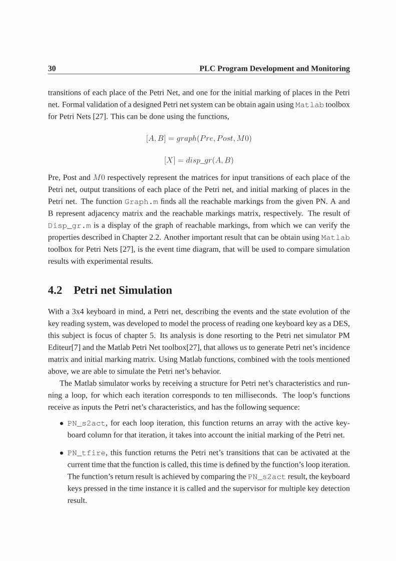
for Petri Nets [27]. This can be done using the functions,
[A,B] = graph(Pre, Post,M0)
[X] = disp_gr(A,B)
Pre, Post andM0 respectively represent the matrices for input transitionsof each place of the
Petri net, output transitions of each place of the Petri net,and initial marking of places in the
Petri net. The functionGraph.m finds all the reachable markings from the given PN. A and
B represent adjacency matrix and the reachable markings matrix, respectively. The result of
Disp_gr.m is a display of the graph of reachable markings, from which wecan verify the
properties described in Chapter 2.2. Another important result that can be obtain usingMatlab
toolbox for Petri Nets [27], is the event time diagram, that will be used to compare simulation
results with experimental results.
4.2 Petri net Simulation
With a 3x4 keyboard in mind, a Petri net, describing the events and the state evolution of the
key reading system, was developed to model the process of reading one keyboard key as a DES,
this subject is focus of chapter 5. Its analysis is done resorting to the Petri net simulator PM
Editeur[7] and the Matlab Petri Net toolbox[27], that allows us to generate Petri net’s incidence
matrix and initial marking matrix. Using Matlab functions,combined with the tools mentioned
above, we are able to simulate the Petri net’s behavior.
The Matlab simulator works by receiving a structure for Petri net’s characteristics and run-
ning a loop, for which each iteration corresponds to ten milliseconds. The loop’s functions
receive as inputs the Petri net’s characteristics, and has the following sequence:
• PN_s2act, for each loop iteration, this function returns an array with the active key-
board column for that iteration, it takes into account the initial marking of the Petri net.
• PN_tfire, this function returns the Petri net’s transitions that canbe activated at the
current time that the function is called, this time is definedby the function’s loop iteration.
The function’s return result is achieved by comparing thePN_s2act result, the keyboard
keys pressed in the time instance it is called and the supervisor for multiple key detection
result.

4.3 Petri net to PLC Conversion 31
• filter_possible_firings, this function compares the result fromPN_tfire
with the marked places from the previous loop iteration or from initial marking, taking
into consideration the Petri net’s incidence matrix. The function returns an array with the
possible transition to be triggered. With this result, the program can now reassign the
marked places array with the marked places result for this loop iteration.
• PN_s2yout, this function checks the marked places array and returns the key pressed
for this loop iteration.
4.3 Petri net to PLC Conversion
Most PLC programmers develop programs using Ladder Logic. In a complex control situation
with a very large number of logical inputs and logical combinations it is difficult to predict the
results of illegal inputs such as damaged input switches or sensors. This lack of control causes
normally stable systems to behave unpredictably.
The approach chosen is however another one, namely using Structured Text (ST), as the
pure text content allows an easier transfer from the Petri net to the PLC integrated development
environment. ST allows to describe the behavior of a controlfunction according to the infor-
mation it receives. Its understanding is simple for users familiar with high-level programming
languages.
4.3.1 Petri net to Structured Text Compiler
The method chosen to transcribe Petri net to ST, creating a PLC program from a Petri Net
and IO mapping, uses three auxiliary functions to that prepare a problem’s specific data, like
timed transitions and physical inputs or outputs, to be usedstraightforward by the main script.
The auxiliary functions enable the following: (1) Load a Petri Net from file, that contains the
incidence matrix and the Petri net’s initial marking; (2) Define the mapping of PLC inputs to PN
transitions, creating a structure with the PLC’s inputs and the selected corresponding transitions,
and with the conflicts between transitions; (3) Define the mapping of PN places to PLC outputs,
creating a structure with the outputs that should change value when the places are marked.
The auxiliary functions, and the main script, used for this method can be seen in Ap-
pendix B.
After having the information provided by our auxiliary functions, we are able to create a
PLC program from a Petri Net and IO mapping using the functions briefly described in the

32 PLC Program Development and Monitoring
following tables.
Functionplc_map_inputs(inp_bits_lst, trans_lst,options)
Input List of mapped transitions.
Output ST code with list of transitions and their respective input.
Description
Allocates one memory position for each transition. Each transition isrepresented by memory position that is the sum of%MW100 plus itstransition number (transition four is%MW104). Establishes causal effectrelation between PLC inputs and memory positions that definetransi-tions.
Table 4.1:plc_map_inputs ST compiler function description.
Function plc_timed_transitions(t_trans_place_lst)
Input List of timed transitions, time out time, list of places.
Output ST code with one timer for each timed transition.
Description
Creates one timer for each timed transition. The activation of the timeris controlled by a place being marked, after the timer reaches timeouttime the transition is triggered. Each of this timed transitions are allo-cated to one memory position.
Table 4.2:plc_timed_transitions ST compiler function description.

4.3 Petri net to PLC Conversion 33
Functionplc_encode_petri_net(pre, pos, mu0, tprio,options)
Input Loaded Petri net.
OutputST code for memory initialization and logical conditions between mem-ory positions
Description
To set the initial condition of the program (initial markingin the Petrinet) it is necessary to create a statement that will be executed only onceby the PLC. The program represents each place by a memory posi-tion that is the sum of%MW200 plus its place number (place four is%MW204). It verifies if initialization command is received, and if so, allthe variables associated to places are set to their initial marking value.Defines cause and effect relations between memory positionsthat de-fine places and memory positions that define transitions, by usingifstatements that check if the memory position for a transition has a valuedifferent than one, and that the memory positions for the places thatneed to be marked for the transition’s firing are marked, if these twoconditions are met, the memory position values are decremented andthe memory positions for the places that receive a mark from the re-ferred transition are incremented.
Table 4.3:plc_encode_petri_net ST compiler function description.

34 PLC Program Development and Monitoring
Functionplc_output_if_any_place(places_lst_main,outp_bit_main)
Input List of mapped places.
Output ST code with list of places and their respective output.
DescriptionThe value of auxiliary variable associated with each place is assigned toits respective output variable, usingif statements. Various places canbe associated with the same PLC output, usingor statements.
Table 4.4:plc_output_if_any_place ST compiler function description.
Function plc_encode_places(places_lst, outp_bits_lst)
Input List of places.
Output ST code to output debug/monitor info.
Description
Create PLC code to output debug / monitor info. Receives a list ofplaces. Usingif, establishes relation between those places beingmarked and a variable (output). It also creates aflag to check ifmore then on of the places in the list e marked. Using bit logicbit logic,and the value from the variableoutput, a bit signal representing themarked place is sent using four outputs.
Table 4.5:plc_encode_places ST compiler function description.

Chapter 5
Case study: Keyboard Reading
Figure 5.1 shows the physical system used in the thesis. The process consists of reading one
keyboard key with a PLC implementing the DES. This section describes the synthesis of the
DES for keyboard reading, taking into account modeling and analysis properties. Synthesis
will be based on supervised control.
Figure 5.1: Plc and terminal.

36 Case study: Keyboard Reading
5.1 Proposed Petri Net Model
Modeling the process of reading one keyboard key as a DES, is done by developing a Petri
Net that describes the events and the state evolution of the key reading system. The developed
system can be divided into tree main blocks. Each block represents one of the tree keyboard
columns. In each of the three blocks there is a wait state, waiting for a key in their column to be
pressed. If a key is pressed the system evolves to a state waiting for the key to be released, and
then the system evolves to the first state, of waiting for a keyto be pressed (same column). The
wait for a key to be pressed state is timed (fifty milliseconds), if a key is not pressed the system
evolves to a wait state for keys from the second column. If again a key is not pressed, after fifty
milliseconds the system evolves to a state of waiting for a key to be pressed on the third column,
if another fifty milliseconds go by, the system evolves againto the first state. A timed transition
(T1, T11 and T2) is used for each of the tree wait states. The activation of different columns is
represented by the marking of one place connected that connect to one of these transitions (P1,
P2 ad P3). If a key is pressed transitions are activated, depending on the key, that pass the mark
to a new place representing the pressed key. A transition connected to each place representing
a pressed key, sends the mark to the wait timed place when a keyis released.
Event Identifier Description
T1Timer controlled transition from actua-tion in keyboard column 1 to column 2
T2Timer controlled transition from actua-tion in keyboard column 3 to column 1
T11Timer controlled transition from actua-tion in keyboard column 2 to column 3
T4, T12, T20 Keyboard key in row 1 pressedT5, T13, T21 Keyboard key in row 2 pressedT6, T14, T22 Keyboard key in row 3 pressedT3, T15, T23 Keyboard key in row 4 pressedT9, T16, T24 Keyboard key in row 1 releasedT10, T17, T25 Keyboard key in row 2 releasedT7, T18, T26 Keyboard key in row 3 releasedT8, T19, T27 Keyboard key in row 4 released
Table 5.1: DES events.
Table 5.1 describes the Petri net events, Table 5.2 shows theconditions for event evolution,
and Table in Figure 5.3 (a) lists the conditions for transition triggering taking into to account the
event evolution. From the event evolution described by the referred tables the incident matrix
on Figure 5.2 is obtained.

5.1 Proposed Petri Net Model 37
Condition Identifier DescriptionP1 column 1 is active, no row is activeP2 column 2 is active, no row is activeP3 column 3 is active, no row is activeP4 column 1 is active, row 4 is activeP5 column 1 is active, row 3 is activeP6 column 1 is active, row 1 is activeP7 column 1 is active, row 2 is activeP8 column 2 is active, row 2 is activeP9 column 2 is active, row 1 is activeP10 column 2 is active, row 3 is activeP11 column 2 is active, row 4 is activeP12 column 3 is active, row 2 is activeP13 column 3 is active, row 1 is activeP14 column 3 is active, row 3 is activeP15 column 3 is active, row 4 is active
Table 5.2: DES conditions.
D =
−1 1 −1 −1 −1 −1 1 1 1 1 0 0 0 0 0 0 0 0 0 0 0 0 0 0 0 0 01 0 0 0 0 0 0 0 0 0 −1 −1 −1 −1 −1 1 1 1 1 0 0 0 0 0 0 0 00 −1 0 0 0 0 0 0 0 0 1 0 0 0 0 0 0 0 0 −1 −1 −1 −1 1 1 1 10 0 1 0 0 0 0 −1 0 0 0 0 0 0 0 0 0 0 0 0 0 0 0 0 0 0 00 0 0 0 0 1 −1 0 0 0 0 0 0 0 0 0 0 0 0 0 0 0 0 0 0 0 00 0 0 1 0 0 0 0 −1 0 0 0 0 0 0 0 0 0 0 0 0 0 0 0 0 0 00 0 0 0 1 0 0 0 0 −1 0 0 0 0 0 0 0 0 0 0 0 0 0 0 0 0 00 0 0 0 0 0 0 0 0 0 0 0 1 0 0 0 −1 0 0 0 0 0 0 0 0 0 00 0 0 0 0 0 0 0 0 0 0 1 0 0 0 −1 0 0 0 0 0 0 0 0 0 0 00 0 0 0 0 0 0 0 0 0 0 0 0 1 0 0 0 −1 0 0 0 0 0 0 0 0 00 0 0 0 0 0 0 0 0 0 0 0 0 0 1 0 0 0 −1 0 0 0 0 0 0 0 00 0 0 0 0 0 0 0 0 0 0 0 0 0 0 0 0 0 0 0 1 0 0 0 −1 0 00 0 0 0 0 0 0 0 0 0 0 0 0 0 0 0 0 0 0 1 0 0 0 −1 0 0 00 0 0 0 0 0 0 0 0 0 0 0 0 0 0 0 0 0 0 0 0 1 0 0 0 −1 00 0 0 0 0 0 0 0 0 0 0 0 0 0 0 0 0 0 0 0 0 0 1 0 0 0 −1
Figure 5.2: Incidence Matrix
µ0 = [1 0 0 0 0 0 0 0 0 0 0 0 0 0 0]T (5.1)
In 5.1 we can see the initial marking for the Petri net places,where the system begins by
waiting for a key to be pressed on column one. The Petri net in Figure 5.3 (b) is the result from
modeling the system of reading a keyboard key. Figure 5.4 is arepresentation of the sequence
of places traversed during the column scanning, when no key is pressed. Thus the columns are
activated in sequence each for fifty milliseconds. In Figure5.5 the Petri net evolution for detec-
tion of a key is shown. The evolution is shown for keyboard keyone, but it would follow similar
sequence of events for all twelve keys for the other keys. These two sequences represent the

38 Case study: Keyboard Reading
Event Pre-Conditions Post-ConditionsT1 P1 P2
T11 P2 P3T2 P3 P1T4 P1 P6T5 P1 P7T6 P1 P5T3 P1 P4T9 P6 P1
T10 P7 P1T7 P5 P1T8 P4 P1
T12 P2 P9T13 P2 P8T14 P2 P10T15 P2 P11T16 P9 P2T17 P8 P2T18 P10 P2T19 P11 P2T20 P3 P13T21 P3 P12T22 P3 P14T23 P3 P15T24 P13 P3T25 P12 P3T26 P14 P3T27 P15 P3
P1
P6 P7
T9
T1
P5 P4
T10 T7 T8
T4 T5 T6 T3
P2
P9 P8
T16
T2
T11
T17 T18 T19
T12 T13 T14 T15
P10 P11
P3
P13 P12
T24 T25 T26 T27
T20 T21 T22 T23
P14 P15
(a) Conditions Table (b) Petri net
Figure 5.3: Table with pre and post conditions for Petri net evolution (a). Developed Petri net(b).
basic operation of the developed Petri net, which correspond to scanning the columns, repeated
during time, and key detection, which will be followed by thescanning state after validation.

5.2 Properties 39
P6 P7
T9
T1
P5 P4
T10 T7 T8
T4 T5 T6 T3
P2
P9 P8
T16
T2 T11
T17 T18 T19
T12 T13 T14 T15
P10 P11
P3
P13 P12
T24 T25 T26 T27
T20 T21 T22 T23
P14 P15
50ms 50ms
50ms
P1
P6 P7
T9
T1
P5 P4
T10 T7 T8
T4 T5 T6 T3
P9 P8
T16
T2 T11
T17 T18 T19
T12 T13 T14 T15
P10 P11
P3
P13 P12
T24 T25 T26 T27
T20 T21 T22 T23
P14 P15
P1
P6 P7
T9
T1
P5 P4
T10 T7 T8
T4 T5 T6 T3
P2
P9 P8
T16
T2 T11
T17 T18 T19
T12 T13 T14 T15
P10 P11
P13 P12
T24 T25 T26 T27
T20 T21 T22 T23
P14 P15
Figure 5.4: Petri net column scanning evolution.
P6 P7
T9
T1
P5 P4
T10 T7 T8
T4 T5 T6 T3
P2
P9 P8
T16
T2 T11
T17 T18 T19
T12 T13 T14 T15
P10 P11
P3
P13 P12
T24 T25 T26 T27
T20 T21 T22 T23
P14 P15
Key 1 Pressed
P1
P7
T9
T1
P5 P4
T10 T7 T8
T4 T5 T6 T3
P2
P9 P8
T16
T2 T11
T17 T18 T19
T12 T13 T14 T15
P10 P11
P3
P13 P12
T24 T25 T26 T27
T20 T21 T22 T23
P14 P15
P6 P7
T9
T1
P5 P4
T10 T7 T8
T4 T5 T6 T3
P2
P9 P8
T16
T2 T11
T17 T18 T19
T12 T13 T14 T15
P10 P11
P3
P13 P12
T24 T25 T26 T27
T20 T21 T22 T23
P14 P15
Key 1 Released
Figure 5.5: Petri net one key pressed evolution.
5.2 Properties
In Section 2.2 properties that provide us a way to characterize Petri Net systems were defined.
These properties are related to the developed Petri net system the following way:

40 Case study: Keyboard Reading
• Reachability, every keyboard key might be pressed.
• Liveness, there are no deadlocks and the continued use of the keyboardis secured.
• Temporal Invariance, the keyboard operation is not degraded with elapsed time.
• Boundedness, the number of possible markings for each place is always thesame.
• Conservation, the number of markings of the entire system stays the same.
• Safeness, only one key is validated at a time.
• Coverability, every system state can be reach from another state, this means there is no
combination of keys that makes another combination of keys unable to be detected.
From equation 2.8, it is known that for in order there needs toexist a triggering vectorq(k)
to go from the markingµ(k) to µ(k + 1), in orderµ(k + 1) be reacheble. The Reachability
Tree, shown in Figure 5.6 has all the reachable markings, andall the transitions that have to be
activated to achieve a certain marking. By analyzing the Reachability Tree, with initial state
µ0 = (1, 0, ..., 0) (corresponding to the beginning column scanning in column 1), it is verified
that the reachability setR(N) is finite and that all other system states are reachable.
From the Reachability Tree, showed if Figure 5.6, we can observe that there are sixteen
different possible markings. From a direct analysis, we observe that for each marking, it is
always possible to define a triggering sequence that will enable any other transition. From this
we can conclude all transitions are live, and from every state you can reach every state, no
deadlock occurs. All the transitions are live of level four.
The conceptual modeling of the keyboard assures temporal invariance to our Petri net. By
sequential scanning and timed column, waiting for a key is pressed, and then returning to the
same column.
A Petri net is k-bounded if all its places are k-bounded. A place is k-bounded if for all
possible states, the number of marks is less than or equal to ainteger k. The developed Petri
net is conservative, the total number of marks remains constant, which ensures that all states
have the same number of marks that the initial state. As the initial state has a mark in place
one (scanning starts in column one), and zero marks in the other places, after each transition,
only one of the places will have a mark and all other places will have zero marks. Therefore, all
places are one bounded and as such, the Petri net is one bounded. It is observable that the Petri
net is safe, since by definition, a Petri net is safe if all its places are one bounded.

5.3 Supervisor 41
t1
(1,0,0,0,0,0,0,0,0,0,0,0,0,0,0,0)
t2
(0,1,0,0,0,0,0,0,0,0,0,0,0,0,0,0)
(0,0,1,0,0,0,0,0,0,0,0,0,0,0,0,0)
(0,0,0,1,0,0,0,0,0,0,0,0,0,0,0,0)
t3
(0,0,0,0,0,0,0,0,0,0,0,0,1,0,0,0)
(1,0,0,0,0,0,0,0,0,0,0,0,0,0,0,0)t25
t13
(0,0,0,0,0,0,0,0,0,0,0,0,0,1,0,0)
(1,0,0,0,0,0,0,0,0,0,0,0,0,0,0,0)t26
t14
(0,0,0,0,0,0,0,0,0,0,0,0,0,0,1,0)
(1,0,0,0,0,0,0,0,0,0,0,0,0,0,0,0)t27
t15
(0,0,0,0,0,0,0,0,0,0,0,0,0,0,0,1)
(1,0,0,0,0,0,0,0,0,0,0,0,0,0,0,0)t28
t16
(1,0,0,0,0,0,0,0,0,0,0,0,0,0,0,0)
t4
(0,0,0,0,0,0,0,0,1,0,0,0,0,0,0,0)
t9
(1,0,0,0,0,0,0,0,0,0,0,0,0,0,0,0)
t21
(0,0,0,0,0,0,0,0,0,1,0,0,0,0,0,0)
t10
(1,0,0,0,0,0,0,0,0,0,0,0,0,0,0,0)
t22
(0,0,0,0,0,0,0,0,0,0,1,0,0,0,0,0)
t11
(1,0,0,0,0,0,0,0,0,0,0,0,0,0,0,0)
t23
(0,0,0,0,0,0,0,0,0,0,0,1,0,0,0,0)
t12
(1,0,0,0,0,0,0,0,0,0,0,0,0,0,0,0)
t24
(0,0,0,0,1,0,0,0,0,0,0,0,0,0,0,0)
t5
(1,0,0,0,0,0,0,0,0,0,0,0,0,0,0,0)
t17
(0,0,0,0,0,1,0,0,0,0,0,0,0,0,0,0)
t6
(1,0,0,0,0,0,0,0,0,0,0,0,0,0,0,0)
t18
(0,0,0,0,0,0,1,0,0,0,0,0,0,0,0,0)
t7
(1,0,0,0,0,0,0,0,0,0,0,0,0,0,0,0)
t19
(0,0,0,0,0,0,0,1,0,0,0,0,0,0,0,0)
t8
(1,0,0,0,0,0,0,0,0,0,0,0,0,0,0,0)
t20
Figure 5.6: Reachability Tree
5.3 Supervisor
In order to eliminate failure in the designed system, due to more than one key being pressed
simultaneously, designing and implementation of a supervisor, that detects the multiple keys
pressed error and resumes the normal operation of the system, is done by applying Supervisory
Control theory.
The Petri net in Figure 5.7, using only two transitions and two places, is used to inform the
system of triggering of multiple keys at the same time, taking the system to a error state. Place
seventeen is used as aflag, that when marked indicates multiple keys are being triggered. In
order to trigger transition twenty eight, the triggering ofmultiple keys must be detected, leading
to the marking of place seventeen. When a non-error state is again reached transition twenty
nine is triggered and place sixteen is marked. On Figure 5.8 the Petri net way of working is
shown. Figure 5.9 shows the incidence matrix for theFlag Petri Net.
To integrate theflag Petri net in Figure5.7, with the Petri net described in section 5.1,
and this way creating a controller to handle the multiple keys pressed error, linear constraints
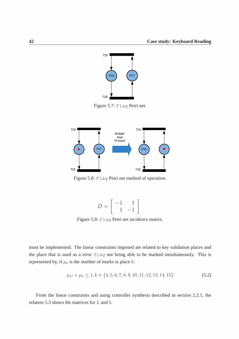
42 Case study: Keyboard Reading
P16 P17
T28
T29
Figure 5.7:Flag Petri net.
P17
T28
T29
P16
T28
T29Multiple
keys Pressed
Figure 5.8:Flag Petri net method of operation.
D =
[
−1 11 −1
]
Figure 5.9:Flag Petri net incidence matrix.
must be implemented. The linear constraints imposed are related to key validation places and
the place that is used as a errorflag not being able to be marked simultaneously. This is
represented by, ifµk is the number of marks in placek:
µ17 + µk ≤ 1, k ∈ {4, 5, 6, 7, 8, 9, 10, 11, 12, 13, 14, 15} (5.2)
From the linear constraints and using controller synthesisdescribed in section 2.2.1, the
relation 5.3 shows the matrices forL andb.

5.3 Supervisor 43
Lµp ≤ b ⇔
⇔
0 0 0 0 0 1 0 0 0 0 0 0 0 0 0 0 1
0 0 0 0 0 0 1 0 0 0 0 0 0 0 0 0 1
0 0 0 0 1 0 0 0 0 0 0 0 0 0 0 0 1
0 0 0 1 0 0 0 0 0 0 0 0 0 0 0 0 1
0 0 0 0 0 0 0 0 1 0 0 0 0 0 0 0 1
0 0 0 0 0 0 0 1 0 0 0 0 0 0 0 0 1
0 0 0 0 0 0 0 0 0 1 0 0 0 0 0 0 1
0 0 0 0 0 0 0 0 0 0 1 0 0 0 0 0 1
0 0 0 0 0 0 0 0 0 0 0 0 1 0 0 0 1
0 0 0 0 0 0 0 0 0 0 0 1 0 0 0 0 1
0 0 0 0 0 0 0 0 0 0 0 0 0 1 0 0 1
0 0 0 0 0 0 0 0 0 0 0 0 0 0 1 0 1
µ1
µ2
µ3
µ4
µ5
µ6
µ7
µ8
µ9
µ10
µ11
µ12
µ13
µ14
µ15
µ16
µ17
6 1(5.3)
The next step in controller synthesis based on linear constraints is verifyingb − Lµp0 ≥ 0,
which is true given that the result ofb − Lµp0 is b. It is relevant to note thatµp0 represents the
initial markings of the combined Petri nets, it is an one column matrix with one row per Petri
net place, seventeen in total, with all values zero except for the first and sixteenth values, which
are one. The first value represents the first state of the keyboard Petri net, waiting for a key
to be pressed for fifty milliseconds, and sixteenth value represents theFlag Petri net state of
multiple keys not being pressed at the same time. The supervisor incidence matrix (Dc) and
initial markings (µc0) are determined by the relations 5.4 and 5.5, respectively.Dp represents
the incidence matrix of the combined Petri nets, it is the result of adding two transitions and
places, rows and columns, to 5.2 with the values of 5.9.

44 Case study: Keyboard Reading
Dc = −LDp =
0 0 0 −1 0 0 0 0 1 0 0 0 0 0 0 0 0 0 0 0 0 0 0 0 0 0 0 −1 1
0 0 0 0 −1 0 0 0 0 1 0 0 0 0 0 0 0 0 0 0 0 0 0 0 0 0 0 −1 1
0 0 0 0 0 −1 1 0 0 0 0 0 0 0 0 0 0 0 0 0 0 0 0 0 0 0 0 −1 1
0 0 −1 0 0 0 0 1 0 0 0 0 0 0 0 0 0 0 0 0 0 0 0 0 0 0 0 −1 1
0 0 0 0 0 0 0 0 0 0 0 −1 0 0 0 1 0 0 0 0 0 0 0 0 0 0 0 −1 1
0 0 0 0 0 0 0 0 0 0 0 0 −1 0 0 0 1 0 0 0 0 0 0 0 0 0 0 −1 1
0 0 0 0 0 0 0 0 0 0 0 0 0 −1 0 0 0 1 0 0 0 0 0 0 0 0 0 −1 1
0 0 0 0 0 0 0 0 0 0 0 0 0 0 −1 0 0 0 1 0 0 0 0 0 0 0 0 −1 1
0 0 0 0 0 0 0 0 0 0 0 0 0 0 0 0 0 0 0 −1 0 0 0 1 0 0 0 −1 1
0 0 0 0 0 0 0 0 0 0 0 0 0 0 0 0 0 0 0 0 −1 0 0 0 1 0 0 −1 1
0 0 0 0 0 0 0 0 0 0 0 0 0 0 0 0 0 0 0 0 0 −1 0 0 0 1 0 −1 1
0 0 0 0 0 0 0 0 0 0 0 0 0 0 0 0 0 0 0 0 0 0 −1 0 0 0 1 −1 1
(5.4)
µc0 = b− Lµp0 = [1 1 1 1 1 1 1 1 1 1 1 1]T (5.5)
The finale incidence matrix of the supervised system (D) is shown in Figure 5.10, the differ-
ent square colors represent the different Petri nets constituting the supervised system. The blue
square outlines the incidence matrix for the Petri net used for key detection from section 5.1, the
green square outlines the incidence matrix for the Petri netused to detect pressing of multiple
keys, the purple square outlines the incidence matrix for the system that combines the last two
referred Petri nets (Dp), and the red square outlines the supervisor controller incidence matrix
synthesized based on linear constraints (Dc). As expected, the application of linear constraints
leads to the appearance of a place (marked on initial state) that links the two Petri nets, ensuring
mutual exclusion for each place in which a key is validated. Thus, there are 12 new places,
initially marked. In 5.6 we can see the final initial marking for the Petri net places, composed of
the initial marking for the original Petri net, the initial marking for the Petri net used to detect
multiple keys, and the initial marking for the supervisor.
The supervised system resulting Petri net is shown in Figure5.11.
µ0 = [1 0 0 0 0 0 0 0 0 0 0 0 0 0 0 1 0 1 1 1 1 1 1 1 1 1 1 1 1]T (5.6)

5.3 Supervisor 45
Figure 5.10: Supervised system incidence matrix.

46 Case study: Keyboard Reading
Figure 5.11: Petri net developed for keyboard control, withsupervisor.

5.4 Implementation 47
5.4 Implementation
Using the ST compiler detailed in 4.3.1 and shown in AppendixB, we are able to implement
the Petri net for our case study in the PLC as ST code.
Using the auxiliary functions for the ST compiler we can: (1)load our Petri Net from
file, containing the incidence matrix, the Petri net’s initial marking, priority transitions (for
our supervisor transitions) and timed transitions; (2) define the mapping of PLC inputs to PN
transitions; (3) Define the mapping of PN places to PLC outputs.
With the results from the auxiliary functions, our compileris then able to create ST code
to run in loop in the PLC, that simulates the work-flow of the developed Petri Net, taking into
account the inputs and outputs received by the PLC. The ST program generate is comprised of
five cyclic operations: (i) Petri net initialization, (ii) PLC input mapping, (iii) controlling timed
transitions, (iv) Petri net loop, (v) setting PLC output, depending of a (vi) encoding of places.
These functions are briefly described in the following paragraphs.
Petri net initialization To set the initial condition of the program (initial markingin our
Petri net) it is necessary to create a statement that will be executed only when an specific input
is received by the PLC. If this condition is met, the valueHIGH must be assigned to all the
auxiliary variables corresponding to the places initiallymarked, and the valueLOW must be
assigned to all the auxiliary variables corresponding to the places with no initial marking. This
correlates to our case study keyboard being in the state of nokeys pressed and with the column
one being the first one to be checked.
To map PLC inputs For each input (that represents a transition) there are two variables, one
to represent theHIGH state of the input and one to represent theLOW state. The variables also
takes into consideration if the output that allows the change of state of an input isHIGH orLOW.
This part of the program checks for keys being pressed or released, and sets the appropriate
value to a variable that represents those actions transition.
Controlling of timed transitions is done with three timers which consecutively, for fifty
milliseconds, set the value of one variable corresponding to a Petri net place toHIGH state.
This are the same transitions used in our Petri net to wait fora key to be pressed for fifty
milliseconds for each column.
The Petri net loop does PLC variables verification. For each scancycle, checkswhich
places should be marked or unmarked. For this, a logical combination (AND) of two conditions
must be performed: (a) input variables associated with the transition are satisfied (HIGH); (b)
existence of tokens in places (auxiliary variables areHIGH). If a transition to another PN state
is possible, the value of place variables is decreased, and the value of the variable representing

48 Case study: Keyboard Reading
the next Place is increased.
Setting PLC outputs is done by checking the values of the created variables and variables
that represent PN Places directly dependent on the first referred variables. It then sets one of
three PLC outputs to aHIGH or LOW level, making possible the interaction of the terminal with
the PLC.
Encoding of placeschecks the value of the PLC variables that represent PN Places are
marked depending on the PLC input, and then outputs a four bitsignal depending on which PN
Place is marked or if more then one Place is marked (error case).

Chapter 6
Experiments
This chapter describes the experiments performed to validate the methodologies presented and
introduced in previous chapters. First, in order to determine various PLC properties, tests are
done, results are explained and illustrated. Next, a simulation of the keyboard reading case
study is done, both by the Petri net simulation program developed for MatLab and by the PLC
receiving key triggering simulation from the monitoring system. In the following section ex-
periments that show the effect of different initial markingto the system Petri net are shown and
discussed. Finally, we present results of the overall system explaining and analyzing results for
cases that involve supervisor control and compare them results obtain by MatLab simulation of
the Petri net.
6.1 PLC Characterization
In a PLC the response to the input from an output is not immediate. PLC’s operate by contin-
ually scanning programs and reading inputs and outputs. Oneiteration of this process is called
scan cycle. The scan cycle consists of three steps: determine status of inputs, interpret logic of
programs, and update output status. Knowing the PLC’s scan cycle is crucial in order to know if
it is going to be fast enough for a particular application. Inthe our particular case, knowing the
scan cycle allows us to know smallest time period possible for the PLC to detect two consec-
utive key triggers. In our experiments the PLC’s scan cycle was fixed to ten milliseconds, this
value was chosen to have a more stable scan cycle, as experiments will show, and because in
the implemented Petri net the minimum value of scan cycle needed for correct operation is fifty
milliseconds. It is also a unrealistic to experiment terminal key pressing for time differences so
low.

50 Experiments
(a) PLC, power supply and Monitor. (b) IO module 28FK.
USB connection
to PC
Generate andmonitor signalsto/from the PLC
Arduidoto PLC adapter
Arduino Mega
I O
PLC
Arduino based
monitor
(c) Monitor. (d) Monitored signal%q0.3.16.
1 %q0 . 3 . 1 6 := NOT(%q0 . 3 . 1 6 ) ;
(e) PLC program
Figure 6.1: Experimental setup for PLC characterization (a). Closeup view of developed mon-itor (b). Closeup view of developed monitor (c). Signal flow diagram for the first experiment(d). PLC square wave generation program (e).
The used experimental setup for this section is shown in Figure 6.1 (a). The setup is com-
posed by the Modicon 28FK PLC (b), the developed signal monitor (c), and a power supply. No
terminal is used for this sections experiments, this is due to the fact that objective in this section
is to be able to acquire PLC characteristics information. Figure 6.1 (d) shows the block diagram
representation of the system used for the PLC’s scan cycle characterization. The PLC’s output
is sends a signal, and the monitor records any changes in the PLC’s output. The structured text
program implemented in the PLC in order to monitor the scan cycle is shown in Figure 6.1
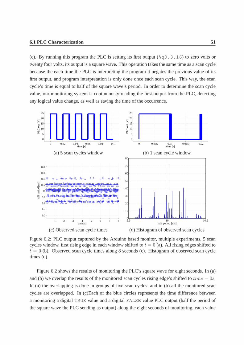
6.1 PLC Characterization 51
(e). By running this program the PLC is setting its first output(%q0.3.16) to zero volts or
twenty four volts, its output is a square wave. This operation takes the same time as a scan cycle
because the each time the PLC is interpreting the program it negates the previous value of its
first output, and program interpretation is only done once each scan cycle. This way, the scan
cycle’s time is equal to half of the square wave’s period. In order to determine the scan cycle
value, our monitoring system is continuously reading the first output from the PLC, detecting
any logical value change, as well as saving the time of the occurrence.
0 0.02 0.04 0.06 0.08 0.1
0
5
10
15
20
25
time [s]
PLC
out
[V]
0 0.005 0.01 0.015 0.02
0
5
10
15
20
25
time [s]
PLC
out
[V]
(a) 5 scan cycles window (b) 1 scan cycle window
1 2 3 4 5 6 7 8
9.2
9.4
9.6
9.8
10
10.2
10.4
10.6
10.8
time [s]
half
perio
d [m
s]
9.5 10 10.50
10
20
30
40
50
60
70
80
half period [ms]
(c) Observed scan cycle times (d) Histogram of observed scancycles
Figure 6.2: PLC output captured by the Arduino based monitor, multiple experiments, 5 scancycles window, first rising edge in each window shifted tot = 0 (a). All rising edges shifted tot = 0 (b). Observed scan cycle times along 8 seconds (c). Histogram of observed scan cycletimes (d).
Figure 6.2 shows the results of monitoring the PLC’s square wave for eight seconds. In (a)
and (b) we overlap the results of the monitored scan cycles rising edge’s shifted totime = 0s.
In (a) the overlapping is done in groups of five scan cycles, and in (b) all the monitored scan
cycles are overlapped. In (c)Each of the blue circles represents the time difference between
a monitoring a digitalTRUE value and a digitalFALSE value PLC output (half the period of
the square wave the PLC sending as output) along the eight seconds of monitoring, each value

52 Experiments
represents a different time of scan cycle. (d) is a graphicalrepresentation of the distribution of
the scan cycle time value, histogram.
From the results shown in Figure 6.2 it is observable that themonitoring system detected that
the PLC output change, does not have an exact time value between occurrences, this time varies
roughly between nine point five milliseconds and ten point five milliseconds. In the context of
our case study, keyboard reading, the interpretation of these results leads us to acknowledge that
a key should not be pressed for less then ten point five milliseconds, or it might not be detected
by the PLC. This is of course also valid for any input we wish thePLC to read.
1 %q0 . 3 . 1 6 := %i 0 . 3 . 0 ;
(a) PLC program.
I O
PLC
Arduino based
monitor
1 2 3 4 5 6 7 89.4
9.6
9.8
10
10.2
10.4
10.6
time[s]
dela
y[m
s]
1 2 3 4 5 6 7 89.4
9.6
9.8
10
10.2
10.4
10.6
time[s]
dela
y[m
s]
9.5 9.6 9.7 9.8 9.9 10 10.1 10.2 10.3 10.4 10.50
20
40
60
80
100
120
140
160
180
half period [ms]
(b) IO signals. (c) Observed delays. (d) Histogram of observed delays.
Figure 6.3: Observing the time from a signal input (rising edge%i0.3.0) to a signal output(rising edge%q0.3.16). PLC input delay test code. (a). Connections diagram (b). ObservedPLC input to output delays along 8 seconds (c) and histogram of the delays (d).
The next PLC characterization test done is for the PLC input delay. We want to be able to
determine the time it takes the PLC to read an input and act on it, input delay. Figure 6.3 (a)
shows the structured text program implemented in the PLC in order to monitor the input delay.
By running this program the PLC is reads one input and attributes the same value from that
input to an output, this is done in loop until the program is told to stop. The monitoring system,
besides monitoring the PLC, starts by sending digitalTRUE value to the PLC’s input, and as
soon as the PLC sets the output to the value of the received input, the monitor starts sending a
digitalFALSE value to the PLC’s input. Again, when the the PLC sets the output to the value of
the received input, the monitoring system starts sending a digital TRUE value to the PLC, this
is done in loop for eight seconds. Representation of this experiment’s connections is shown in
Figure 6.3 (b).
Figure 6.3 (c) and (d) shows the results of monitoring the PLC’s output while the monitoring
system is changing its input for eight seconds. In (a) each ofthe blue circles represents a time

6.1 PLC Characterization 53
delay, the time difference between a monitoring a digitalTRUE value and a digitalFALSE value
from the PLC output along the eight seconds of monitoring. In(d) a graphical representation of
the distribution of the delay time values is shown, histogram.
From Figure 6.3 results we can see that the PLC input delay time is not exact, but in fact
varies roughly between nine point five milliseconds and ten point five milliseconds. The delay
input results are similar to the scan cycle results. This is in fact expected, since the monitoring
is actually changing its output after the PLC runs a full scancycle. With this results we are
able to verify that the fact that the PLC is in fact receiving input information does not change
significantly the scan cycle time. This results reinforce the fact that in our case study, keyboard
reading, a key should not be pressed for less then ten point five milliseconds, or it might not be
detected by the PLC.
I O
PLC
50ms
100ms
10Hz
Time difference of
rising and falling edges
0 1 2 3 4 5 6 7 8
40
42
44
46
48
50
52
54
56
58
60
time [s]
half
perio
d [m
s]
(a)IO signals. (b) Input Detection
Figure 6.4: Observing the time for 100ms period square signal detection. Connections diagram(a). Observed PLC time of signal detection along 8 seconds (b).
One more characterization experiment was done running the same PLC structured text pro-
gram implemented in the previous experiment. But in this case, the monitoring system is not
only monitoring the PLC’s inputs and outputs, but it is also generating a square wave signal with
a period of one hundred milliseconds. The PLC should set its output according to the value it is
receiving in its input (digitalTRUE or FALSE), the received square wave value. In Figure 6.4
(a) a block diagram for this experiment is shown.
From the results shown in Figure 6.4 (b) we observe that the monitoring system detected
the PLC output change in the expected time instances, fifty milliseconds apart (half the period
time). We can also observe that time of input detection is notexact, this is justifiable by the
previous experiments, where it was shown that the scan cycletime is not exact and has values

54 Experiments
with differences of up to one millisecond from each other. The results also show some increase
in input detection, of almost ten milliseconds. This can be seen in Figure 6.4 (b) around the
time mark of four and a half seconds. This happens when the PLCfails to detect an input
change, and only detects it in its next scan cycle, thus the increase of ten milliseconds. The
forty milliseconds time change shown in the results, happens because an input was detected late
by the PLC, so the time difference of the next correctly detected input should be detected ten
milliseconds earlier. The fact that there are two input detections at sixty milliseconds since the
last inputs, but only one forty milliseconds input detection since the last input, can be attributed
to two straight input detection delays by the PLC.
0 1 2 3 4
x 10−3
0
5
10
15
20
25
time [s]
PLC
out
[V]
0 1 2 3 4
x 10−3
0
5
10
15
20
25
time [s]
PLC
out
[V]
(a) Minimum time observed. (b) Maximum time observed.
Figure 6.5: Varying scan cycle time. Minimum scan cycle timeobserved experimentally (a).Maximum scan cycle time observed experimentally (b).
In the context of our case study, keyboard reading, the interpretation of previous results leads
us to acknowledge that the PLC set to a ten millisecond time ofscan cycle has an accuracy with
an error of plus and minus ten milliseconds. Figure 6.5 showsthe minimum (a) and maximum
(b), time difference between rising edges, of monitoring time of scan cycle, as it was done in
the first experiment (results shown in Figure 6.2), but with the difference that this results were
obtained without a PLC fixed scan cycle time of ten milliseconds. As shown in Figure 6.5, the
PLC can have a scan cycle of less then one millisecond, but thevariation of time of scan cycle
increases greatly, leading to detected change in scan cycletime of around three milliseconds.
Since there is no need in our case study, to have a scan cycle lower than ten milliseconds, and
since not assigning a fixed value to the PLC’s time of scan cycleleads to a more unstable scan
cycle time, the ten milliseconds time of scan cycle was sustained in experiments done in the
next sections.

6.2 Key detection 55
IDC connectionto Monitor
(a) Generic setup. (b) Terminal.
Figure 6.6: Setup used for experiments. Setup for monitoring PLC (a). Keyboard terminal (b).
6.2 Key detection
This experiment carried out a sequential triggering and release of all the keys, without conflicts.
The used experimental setup for this section is shown in Figure 6.6 (a). The setup is composed
by the Modicon 28FK PLC (with the developed Petri net implementation code detailed in sec-
tion 5.4), the developed signal monitor, a power supply, andthe twelve key keyboard terminal.
The terminal and PLC are directly connected to the monitor each thru a insulation-displacement
connector cable. The monitor records all the inputs it receives. The key triggering is actually
done by signals sent by the monitor, the terminal is only usedfor the confirmation that the cor-
rect column is activated, was explained in section 5.4. Thisway we can trigger keys at the exact
time, and during the exact duration of time we want, conditions which are essential in order for
us to be able to compare experimental results to Matlab simulation results.
The key sequence used, during a time period of eighteen seconds (input data), is shown in
Figure 6.7 (a). In Table (b), besides the key sequence used, also includes the period of time
in which the keys are triggered and the expected results the PLC should output. Figure 6.7
(c) shows the Matlab simulation (that simulates the complete Petri net that reads keys) results
using the input data for this experiment. Figure 6.7 (d) shows the PLC monitoring results for
the same input data. We can also observe that in the monitoring results the PLC does not output
any error bit sequence (error sequence for multiple key detection). The experimental results are
consistent with the Matlab simulation results, as well as with the expected results.
This experiment, by input and output monitoring, shows thatthe correct validation of key
triggering and release of all the keys, without conflicts, iscorrectly done by the the Petri net
implemented in the PLC.

56 Experiments
0 1 2 3 4 5 6 7 8 9 10 11 12 13 14 15 16 17 18
key 1
key 2
key 3
key 4
key 5
key 6
key 7
key 8
key 9
key 10
key 11
key 12
time[s]0 1 2 3 4 5 6 7 8 9 10 11 12 13 14 15 16 17 18
key 1
key 2
key 3
key 4
key 5
key 6
key 7
key 8
key 9
key 10
key 11
key 12
time[s]
Time Key Inputs Expected Result0 - -1 1 12 - -3 2 24 2 25 3 36 - -7 4 48 5 59 6 610 7 711 - -12 8 813 9 914 10 1015 11 1116 - -17 12 12
(a) Input data, pressed keys. (b) Expected results given theinput data.
0 1 2 3 4 5 6 7 8 9 10 11 12 13 14 15 16 17 18
key 1
key 2
key 3
key 4
key 5
key 6
key 7
key 8
key 9
key 10
key 11
key 12
time[s]0 1 2 3 4 5 6 7 8 9 10 11 12 13 14 15 16 17 18
key 1
key 2
key 3
key 4
key 5
key 6
key 7
key 8
key 9
key 10
key 11
key 12
time[s]1 2 3 4 5 6 7 8 9 10 11 12 13 14 15 16 17 18
Errors
key 1
key 2
key 3
key 4
key 5
key 6
key 7
key 8
key 9
key 10
key 11
key 12
time[s]1 2 3 4 5 6 7 8 9 10 11 12 13 14 15 16 17 18
Errors
key 1
key 2
key 3
key 4
key 5
key 6
key 7
key 8
key 9
key 10
key 11
key 12
time[s]
(c) Expected output, MatLab simulation. (d) Monitoring experiment results.
Figure 6.7: PLC output captured by the Arduino based monitor, input data key sequence (a).Input data, sequence of keys (b). Expected output, MatLab Simulation (c). PLC output observedwith the developed monitor (d).
6.3 Initial Marking Effect
The experiments done in this section carried out a sequential triggering and release of all the
keys. For each experiment, a different Petri net initial marking was used. The experimental
setup used in this section’s experiments is connected the same way as in the previous section,
as well as follows the same operation method, and again is composed by the Modicon 28FK
PLC, the developed signal monitor, a twenty four volts DC power supply, and the twelve key
keyboard terminal.
Initial marking of the implemented Petri net is expected to have an effect to our system in
the way it validates one of multiple keys triggered at the same time from difference terminal
keyboard columns. When initialized, the Petri net has a mark in one of the three places that

6.3 Initial Marking Effect 57
represent column activation, if fifty milliseconds go by andno key is pressed, a timed transition
transfers the marking to the next column activation place. This way, if multiple keys from
different columns are pressed, the key validated will be theone belonging to column which has
its Petri net place marked.
0 1 2 3 4 5 6 7 8 9 10 11 12 13 14 15 16 17 18
key 1
key 2
key 3
key 4
key 5
key 6
key 7
key 8
key 9
key 10
key 11
key 12
time[s]0 1 2 3 4 5 6 7 8 9 10 11 12 13 14 15 16 17 18
key 1
key 2
key 3
key 4
key 5
key 6
key 7
key 8
key 9
key 10
key 11
key 12
time[s]
(a) Input data, multiple keys pressed at the same time.µ0 =
[
1 0 0 0 0 0 0 0 0 0 0 0 0 0 0 1 0 1 1 1 1 1 1 1 1 1 1 1 1]T
(b) Initial marking.
(c) Expected output, MatLab Simulation. (d) PLC output observed with the developed monitor.
Figure 6.8: PLC output captured by the Arduino based monitor, input data key sequence (a).Initial marking of Petri net (b). Expected output, MatLab Simulation (c). PLC output observedwith the developed monitor (d).
The key sequence used for all the experiments in this section, during a time period of eigh-
teen seconds (input data), is shown in Figure 6.8 (a). Three keys from different columns are
pressed at the same time, in different time instances (zero,three, seven and thirteen seconds). In
(b) is shown the first used initial marking matrix. With this initial marking, when the Petri net is
initialized, the place in which the the system waits for a keyto be pressed on the first column for

58 Experiments
fifty milliseconds is marked. The supervisor configuration of places that indicate that no multi-
ple from the same column are also marked. Figure 6.8(c) showsthe Matlab simulation results
using the input data for this experiment. Figure 6.8(d) shows the PLC monitoring results for the
same input data. The experimental results are consistent with the Matlab simulation results. As
expected, the results show that in the first time instance of pressed keys, the key validated is the
one that belongs to the initial marked column (first column),key one.
µ0 =[
0 0 1 0 0 0 0 0 0 0 0 0 0 0 0 1 0 1 1 1 1 1 1 1 1 1 1 1 1]T
(a) Initial marking.
(b) Expected output, MatLab Simulation. (c) PLC output observed with the developed monitor.
Figure 6.9: PLC output captured by the Arduino based monitor, initial marking of Petri net (a).Expected output, MatLab Simulation (b). PLC output observed with the developed monitor (c).
In Figure 6.9(a) is shown the initial marking matrix used forthis section’s second exper-
iment. With this initial marking, when the Petri net is initialized, the place in which the the
system waits for a key to be pressed on the third column for fifty milliseconds is marked. The
supervisor configuration of places that indicate that no multiple from the same column are also
marked. Figure 6.9(c) shows the Matlab simulation results using the input data for this experi-
ment. Figure 6.9(d) shows the PLC monitoring results for thesame input data. The experimental
results are consistent with the Matlab simulation results.As expected, the results show that in
the first time instance of pressed keys, the key validated is the one that belongs to the initial
marked column (third column), key three. Comparing these results with the ones on the last
experiment we also observe that the rest of the validated keys don’t match, this is also expect,
since the fact that the initialization is done in different columns, with the passage of time, the
column activation for each column will be done in different time instances.
In Figure 6.10(a) is shown the initial marking matrix used for this section’s third experiment.
With this initial marking, when the Petri net is initialized, the place that represents the trigering

6.4 Supervisory Control 59
µ0 =[
0 0 0 0 0 0 0 0 0 1 0 0 0 0 0 1 0 1 1 1 1 1 1 1 1 1 1 1 1]T
(a) Initial marking.
(b) Expected output, MatLab Simulation. (c) PLC output observed with the developed monitor.
Figure 6.10: PLC output captured by the Arduino based monitor, initial marking of Petri net(a). Expected output, MatLab Simulation (b). PLC output observed with the developed monitor(c).
and validation of keyboard key number ten is marked. The supervisor configuration of places
that indicate that no multiple from the same column are also marked. Figure 6.10(c) shows
the Matlab simulation results using the input data for this experiment. Figure 6.10(d) shows the
PLC monitoring results for the same input data. The experimental results are consistent with the
Matlab simulation results. This experiment differs from the previous two, because the Petri net
is initialized with a key already validated. This however does will take an extra scan cycle until
the system learn that in fact no key is pressed, going back to waiting for a key to be pressed,
this time in column two, since this is the column the validation of key eight must be active.
Knowing this, as expected, the results show that in the first time instance of pressed keys, the
key validated belongs to the second column, key two. Comparing these results with the ones
on the last experiments we also observe that the rest of the validated keys don’t match, this is
also expect, since the fact that the initialization is done in different columns, with the passage
of time, the column activation for each column will be done indifferent time instances.
6.4 Supervisory Control
In this section we present the results concerning the implementation, to the design Petri net, of
a supervisor based in linear constraints, done in section 5.3, in order to prevent failure in the
designed system, due to more than one key being pressed simultaneously. It is our objective to

60 Experiments
successfully test various keyboard inputs, leading to situations where the supervisor is crucial
for proper operation of the implemented Petri net system. Inorder to simulate keyboard key
pressing and release, and to monitor PLC results, the developed monitoring system (powered by
a DC power supply) connected to a PC was used, as well the system terminal. The experimental
setup is the same used in section 6.2.
0 1 2 3 4 5 6 7 8 9 10 11 12 13 14 15 16 17 18
key 1
key 2
key 3
key 4
key 5
key 6
key 7
key 8
key 9
key 10
key 11
key 12
time[s]0 1 2 3 4 5 6 7 8 9 10 11 12 13 14 15 16 17 18
key 1
key 2
key 3
key 4
key 5
key 6
key 7
key 8
key 9
key 10
key 11
key 12
time[s]
Time Key Inputs Expected Result0 1 11 - -2 - -3 - -4 - -5 - -6 - -7 - -8 2, 8 Error9 - -10 - -11 - -12 - -13 5 514 - -15 - -16 - -17 - -
(a) Input data, pressed keys. (b) Expected results given theinput data.
0 1 2 3 4 5 6 7 8 9 10 11 12 13 14 15 16 17 18
key 1
key 2
key 3
key 4
key 5
key 6
key 7
key 8
key 9
key 10
key 11
key 12
time[s]0 1 2 3 4 5 6 7 8 9 10 11 12 13 14 15 16 17 18
key 1
key 2
key 3
key 4
key 5
key 6
key 7
key 8
key 9
key 10
key 11
key 12
time[s]0 1 2 3 4 5 6 7 8 9 10 11 12 13 14 15 16 17 18
Errors
key 1
key 2
key 3
key 4
key 5
key 6
key 7
key 8
key 9
key 10
key 11
key 12
time[s]0 1 2 3 4 5 6 7 8 9 10 11 12 13 14 15 16 17 18
Errors
key 1
key 2
key 3
key 4
key 5
key 6
key 7
key 8
key 9
key 10
key 11
key 12
time[s]
(c) Expected output for supervisor experiments,MatLab simulation.
(d) Monitoring supervisor experiment results.
Figure 6.11: PLC output captured by the Arduino based monitor, input data key sequence (a).Input data, sequence of keys (b). Expected output, MatLab Simulation (c). PLC output observedwith the developed monitor (d).
The first experiment in this section, is done to verify if the supervisor implementation is
working properly, preventing system failure due to multiple keys from the same column being
pressed at the same time. Taking this into consideration, itis not expected that any key is
validated, on the contrary, an error state should be monitored by the system implemented in the
PLC.

6.4 Supervisory Control 61
Figure 6.11 (a) shows the key combinations being pressed andreleased by the developed
monitoring system, during a time period of eighteen seconds(input data). The table (b) in
the same Figure shows the expected results for each time instant. Figure 6.11 (c) shows the
Matlab simulation results from the input data mentioned above. Figure 6.11 (d) shows the PLC
monitoring results for the same input data. Both results are consistent with the expected results,
and with each other. The supervisor detects triggering of multiple keys and does not validate any
of them. In the Matlab simulation that single keys being pressed during the time of experiment
are validated, but when the system receives multiple keys from the same column, eight seconds
time mark, no key is validated. In the monitoring results, nokey validated in the eight seconds
time instance, and we can also observe that the PLC outputs the error bit sequence as mentioned
in section 5.4. This error sequence is received multiple times during the referred time instance,
this is due to the fact that the PLC keeps receiving, from the monitoring system, the same key
triggering information for every scan cycle it does during the said time period.
To further experiment the supervisor implantation severaltest were conceived. The key-
board inputs done in order to test the supervisor implementation were the following:
i) Three keys from the same keyboard column are pressed at theinstant of time, and are
released after one second.
ii) Two keys from the different keyboard columns are pressedat the same instant of time.
After one second, one key is released and the other stays pressed for one more second.
iii) One key is pressed, after one second two more keys, from the same column of the first key,
are pressed (the first key remains pressed). The three keys remain pressed for two seconds,
except for the first pressed key which remains pressed for onemore second after the others
have been released.
iv) Two keys from the same keyboard column are pressed at the same instant of time. After
one second, one key is released and the other stays pressed for one more second.
Figure 6.12 (a) shows the key combinations being pressed andreleased by the developed
monitoring system, during a time period of eighteen seconds(input data). The supervisor tests
referred above are outlined by green rectangles, with the test specific identifying letter beneath
them. The table from Figure 6.12 (b) shows the expected results for each time instant.
The first test, i), is done to check if the main reason for supervisor implementation is working
properly, prevention of system failure due to multiple keysfrom the same column being pressed
at the same time. Taking this into consideration, it is not expected that any key is validated, on
the contrary, an error state should be monitored by the system implemented in the PLC.

62 Experiments
a)
b)
c)
d)
Time Key Inputs Expected Result0 - -1 5 52 - -3 2 24 1, 4, 7 Error5 - -6 2, 6 2 or 67 6 68 2 29 2 210 9 911 3, 9, 12 Error12 3, 9, 12 Error13 9 914 - -15 2, 11 Error16 11 1117 - -
(a) Input data, pressed keys, including variouscases of simultaneous keys (green rectangles).
(b) Expected results given the input data.
a)
b)
c)
d)
a)
b)
c)
d)
(c) Expected output for supervisor experiments,MatLab simulation.
(d) Monitoring supervisor experiment results.
Figure 6.12: PLC output captured by the Arduino based monitor, multiple experiments, inputdata key sequence (a). Input data, sequence of keys (b). Expected output, MatLab Simulation(c). PLC output observed with the developed monitor (d).
In test ii) although multiple keys are being pressed, since they are not in the same keyboard
column, it is expected that one of the two keys is validated, taking into account the fact the im-
plemented Petri net cyclically checks for key triggering for each column, and that the supervisor
only checks for key triggering conflicts for in the active column.
Test iii) serves the purpose of proving that in a case where a key is already validated, the
fact that in a future time instance keys from the same column are pressed, does not make the
enter a error state. In fact the supervisor keeps the previous key validated until said key is not
being pressed.
On test iv) the opposite of test iii) is being checked. Two keys from the same column are

6.4 Supervisory Control 63
triggered, making the supervisor take the system to error state, and in the next instance of time
one of the two keys is released. The proper response from the system should be leaving the
error state and validating the key that remains pressed.
Figure 6.12 (c) shows the Matlab simulation results from theinput data mentioned above.
Figure 6.12 (d) shows the PLC monitoring results for the sameinput data. The results from
tests done to detect supervisor behavior are outlined by green rectangles, with the test specific
identifying letter beneath them. Both results are consistent with the expected results, and with
each other.
Test i) result is consistent with expected results. The supervisor in fact detects triggering of
multiple keys and does not validate any of them. In the Matlabsimulation this is represented
by no key being ON in the time instance from four to five seconds. In the monitoring results,
not only is no key ON in the four to five seconds time instance, but we can also observe that
the PLC outputs the error bit sequence as mentioned in section 5.4. This error sequence is
received multiple times during the referred time instance,this is due to the fact that the PLC
keeps receiving, from the monitoring system, the same key triggering information for every
scan cycle it does during the said time period.
In test ii), as intended, the supervisor does not interfere with key validation. This is ob-
servable in both the Matlab simulation and the PLC monitoring results. As said, since the keys
pressed are not the same column the key validated is the one that is part of the column the Petri
net implemented system is scanning, or from the next column to be scanned that contains a
pressed key, in case none of the keys pressed are from the currently being scanned column.
Test iii) is also consistent with expected results, for boththe Matlab simulation and the PLC
implementation. At time equals ten seconds key nine is triggered, and as it can be observed
in both the result Figures, it stays validated until it is released in time equals fourteen seconds.
Although more keys from the same column as key nine are triggered in the instance of time
from eleven to thirteen, since a key is already validated, and is not released, the system doesn’t
go into error state. This is actually proven by the fact that the PLC does not output any error bit
sequence for the entire period of time from ten to fourteen seconds.
The last test, test iv), was again a success in terms of agreement between expected, simu-
lation and experimental results. In the Matlab simulation results it is observable that no keys
are validated for the time period keys from the same column are pressed, fifteen to sixteen sec-
onds, and in the exact next time instance when a one of the keysis released, the one that stays
pressed is validated until it is released one second after, meaning that the supervisor detected
the problem while it lasted. This is also observable for the PLC monitoring results, with the
added result that the PLC outputs the error state bit sequence numerous time during the fifteen

64 Experiments
to sixteen time period, each one of those time representing ascan cycle done by the PLC that
continues to detect the same key configuration.
The experimental results obtained in this section prove that the implemented supervisor
works as it was designed to. It is worth mentioning that inputdata for single keys is sent
between the supervisor tests, as it can the seen in Figure 6.12 (a), in order to observe that keys
triggered before or after the events leading to the discussed tests do not interfere with the correct
behavior of the implemented supervisor.

Chapter 7
Conclusion and Future Work
The work described in this thesis is focused in the implementation and implementation-validation
of a discrete event system (DES). The validation is based in adeveloped signal acquirer for PLC
signal inputs and outputs.
We first presented a form of DES representation, Petri nets, aintuitive method that captures
structural information about the system and has mathematical analysis techniques well devel-
oped. This proved to be an effective way to represent our casestudy. We were able to create
the intended system as a Petri net and, using supervising methodologies, we were able to avoid
accepting multiple same-column keys at the same time.
We have developed a signal acquirer, based in the low-cost microcontroller board Arduino
Mega, that can observe and save in memory signals going from and to a PLC connected to a
terminal, and at the same time is able to connect to a PC for further data processing or logging.
More in detail, the signal acquirer is able to act as the terminal, mimicking its behavior by
sending signals to the PLC. In order to achieve this we developed an Arduino shield that is able
to ensure the connections between the Arduino, the PLC and the terminal.
To implement a DES in a PLC, in the form of Petri net representation, we chose to create
a program that produces structured text code. Implementinga Petri net in a device usually re-
quires discrete events, but may also require timed events. To develop the conversion program
we add to take into consideration not only the Petri net relationships between places and tran-
sitions, but we had to take into consideration the assuranceof having a way to initialize the
implemented Petri net in the desired configuration. In addition, we had to define connections
between signal inputs and outputs with the various PLC memory positions attributed to the Petri
net places and transitions.
In summary, besides the central function converting code from a Petri net structure to struc-

66 Conclusion and Future Work
tured text, four other functions had to be created. These points are also valid for the Petri net
simulator used to obtain results about the Petri net development along a time period.
The case studied in chapter 5 showed that, although a Petri net being a good way to represent
a DES, its standard form does not take into consideration some aspects. One of those aspects
is that a PLC is based in scan cycles which constrain the activation speed of transitions. We
also observed in the experiments that a PLC is also subject todelay of signal change detection,
which is another aspect that a Petri net does not take into consideration.
Concluding, the Petri net modeling proved to be effective. Wewere able to obtain a working
system for the proposed case study. The supervisor implementation was also successful, in the
sense that applied the desired constraints. However, even thought we were able to predict to a
large extent the experimental results, the experiment consisting of changing the initial marking
of a Petri net, proved that a DES implementation into a real world situation has more details
that have to be taken into consideration than those presented by a Petri net.
Future work should focus on further development of the Arduino based shield. Ways to not
bind each of the Arduino’s inputs and outputs to one signal can be implemented using integrated
circuits that can send send signals to multiple lines at the same time, by only receiving signal
from one source. This would make it possible to use a even lower-cost version of the Arduino
board.
Another aspect that should be developed, is the DES representation. The use of a more
advanced Petri net representation, I/O Petri net, can lead to a more detailed DES representation,
with fewer aspects that affect its implementation.

Appendix A
Arduino Shield for IO Monitoring
This appendix presents the circuit diagram and PCB schematicfor an Arduino Mega shield,
developed as part of this thesis signal acquirer. Section 3.3 details the development of the
referred signal acquirer.

68 Arduino Shield for IO Monitoring
Figure A.1: Arduino shield electronic schematic.

69
Figure A.2: Arduino shield PCB schematic.
Figure A.3: Arduino shield physical PCB, front.

70 Arduino Shield for IO Monitoring
Figure A.4: Arduino shield physical PCB, back.

Appendix B
PN to PLC Compiler Usage
This Appendix shows the usage of PN to PLC compiler functions, introduced in section 5.4,
applied to the case study detailed in chapter 5.
The compiler functions are called in the main script shown infig. B.1.
In this appendix are also listed the auxiliary functions that prepare all problem specific data,
like timed transitions and physical inputs or outputs, to beused straightforward by the main
script. More in detail, the auxiliary functions do: (i) loadthe Petri net, including priority and
timed transitions, see fig. B.2, (ii) define the mapping of PLC inputs to PN transitions, see
fig. B.3 and (iii) define the mapping of PN state to PLC outputs, see fig. B.4.
In order to help observing the state of the PN running in the PLC, 13 places of the PN are en-
coded as 4 output bits of the PLC. See the call ofplc_encode_places in the main script and
the definition ofplaces_to_show in the auxiliary functiondefine_output_mapping.
The result of the main script, the complete ST program created, is listed in appendix C.

72 PN to PLC Compiler Usage
1 f unc t i on make_PLC_program23 % load t h e P e t r i Net f rom f i l e4 [ pre , pos , mu0 , t p r i o , t t i m e d ]= l o a d _ P e t r i _ N e t ;56 % Create PLC code t o map PLC i n p u t s t o PN t r a n s i s t i o n s7 inp_map= d e f i n e _ i n p u t _ m a p p i n g ;8 p r g _ t f i r e = p l c_map_ inpu ts ( inp_map ) ;9
10 % Create PLC code t o make t imed t r a n s i t i o n s ( f i r e a f t e r t i m e ou t s )11 p r g _ t t r a n s = p l c _ t i m e d _ t r a n s i t i o n s ( t t i m e d ) ;1213 % Create PLC code t o run t h e P e t r i Net14 [ p rg_pn_ in i , prg_pn ]= p l c _ e n c o d e _ p e t r i _ n e t ( pre , pos ,mu0 , t p r i o ) ;1516 % Create PLC code t o map PN p l a c e s t o PLC o u t p u t s17 [ output_map , p laces_ to_show ]= de f i ne_ou tpu t_mapp ing;18 p r g _ a c t = p l c _ o u t p u t _ i f _ a n y _ p l a c e ( output_map ) ;1920 % Create PLC code t o o u t p u t debug / mon i to r i n f o21 prg_you t = p l c _ e n c o d e _ p l a c e s ( p laces_ to_show {1} , p laces_ to_show { 2 } ) ;2223 % Save a l l code t o a t e x t f i l e24 ofname= ’ t s t_mk_prog ram_res . t x t ’ ;25 f p r i n t f ( 1 , ’−− Wr i t i ng "%s " . . . ’ , ofname ) ;26 t e x t _ w r i t e ( ofname , . . .27 p rg_pn_ in i , . . .28 p r g _ t f i r e , . . .29 p r g _ t t r a n s , . . .30 prg_pn , . . .31 p rg_ac t , . . .32 p rg_you t )33 f p r i n t f ( 1 , ’ done . \ n ’ ) ;3435 re turn
Figure B.1: Create a PLC program from a Petri Net and IO mapping.
1 f unc t i on [ pre , pos , mu0 , t p r i o , t t i m e d ]= l o a d _ P e t r i _ N e t23 [D, mu0 ] = g e n e r a t e _ c o n t r o l l e d _ p e t r i ( ’ p l a n t _ s u p e r v i s or . mat ’ ) ;4 [ pre , pos ] = PN_decomp (D) ;% s p l i t D i n t o D+ ( pos ) and D− ( pre )5 t p r i o = [28 2 9 ] ; % t r a n s i t i o n s 28 and 29 have p r i o r i t y6 T= 50e−3; % 50 m i l i s e c o n d s t i m e o u t7 t t i m e d = [T 1 1 ; T 11 2 ; T 2 3 ] ;89 re turn
Figure B.2: Load a Petri Net from file.

73
1 f unc t i on inp_map= d e f i n e _ i n p u t _ m a p p i n g23 % d e f i n e r e c e p t i v i t y f u n c t i o n s4 % ( f i r s t d e f i n e a u x i l i a r y f u n c t i o n s )5 neg_mk = @( x)(−x−100);6 inp_and = @( a , b ) [ a ; 0∗a+b ] ;78 inp_map= { . . .9 inp_and ( 0 : 3 , 4 ) , [4 5 6 3 ] ; . . .
10 inp_and ( neg_mk ( 0 : 3 ) , 4 ) , [9 10 7 8 ] ; . . .11 inp_and ( 0 : 3 , 5 ) , 1 2 : 1 5 ; . . .12 inp_and ( neg_mk ( 0 : 3 ) , 5 ) , 1 6 : 1 9 ; . . .13 inp_and ( 0 : 3 , 6 ) , 2 0 : 2 3 ; . . .14 inp_and ( neg_mk ( 0 : 3 ) , 6 ) , 2 4 : 2 7 ; . . .15 neg_mk ( 7 ) , 0 } ; % i n p u t 7 => PN/ PLC r e s e t1617 mul t iKeyTrue= s t r u c t ( ’ op ’ , ’OR_of_ANDs ’ , ’ t r a n s I d ’ ,28 , . . .18 ’ l s t ’ , { { [0 1 ] , [0 2 ] , [0 3 ] , [1 2 ] , [1 3 ] , [2 3 ] } } ) ;19 inp_map {end+1 ,1}= mul t iKeyTrue ;2021 mu l t iKeyFa l se = s t r u c t ( ’ op ’ , ’NOR_of_ANDs ’ , ’ t r a n s I d ’,29 , . . .22 ’ l s t ’ , { { [0 1 ] , [0 2 ] , [0 3 ] , [1 2 ] , [1 3 ] , [2 3 ] } } ) ;23 inp_map {end+1 ,1}= mu l t iKeyFa l se ;2425 re turn
Figure B.3: Define the mapping of PLC inputs to PN transitions.
1 f unc t i on [ output_map , p laces_ to_show ]= de f i ne_ou tpu t_mapp ing23 % d e f i n e o u t p u t b i t s e s s e n t i a l f o r t h e sys tem t o work4 % PN p l a c e s 1 , 2 , 3 , 4 : 7 , 8 : 1 1 , 1 2 : 1 5 imp ly PLC o u t p u t s 16 ,17 ,185 %6 col1_ON= [ 1 , 4 : 7 ] ;7 col2_ON= [ 2 , 8 : 1 1 ] ;8 col3_ON= [ 3 , 1 2 : 1 5 ] ;9 output_map= {col1_ON , 16 ; col2_ON , 17 ; col3_ON , 18} ;
1011 % d e f i n e o u t p u t b i t s f o r sys tem s t a t e o b s e r v a t i o n / debug purposes12 % i n t h e f o l l o w i n g example t h e r e are 13 PN p l a c e s (−1 v a l u e s are igno red )13 % t o be mapped as 4 o u t p u t b i t s 24:2714 %15 p laces_ to_show {1}= [6 9 13 7 8 12 5 10 14 4 11 15−1 −1 1 7 ] ;16 p laces_ to_show {2}= [ 2 4 : 2 7 ] ;1718 re turn
Figure B.4: Define the mapping of PN places to PLC outputs.

74 PN to PLC Compiler Usage

Appendix C
PLC Program
The PLC Structured Text program listed in this appendix is the implementation of the solution
of the case study presented in chapter 5. The program was generated by the main script listed
in appendix B.
1
2 (∗ −−− PNC: P e t r i n e t i n i t i a l i z a t i o n −−− ∗ )
3
4 IF %MW100=0 THEN
5 %MW201: = 1 ; %MW202: = 0 ; %MW203: = 0 ; %MW204: = 0 ; %MW205: = 0 ;%MW206: = 0 ;
6 %MW207: = 0 ; %MW208: = 0 ; %MW209: = 0 ; %MW210: = 0 ; %MW211: = 0 ;%MW212: = 0 ;
7 %MW213: = 0 ; %MW214: = 0 ; %MW215: = 0 ; %MW216: = 1 ; %MW217: = 0 ;%MW218: = 1 ;
8 %MW219: = 1 ; %MW220: = 1 ; %MW221: = 1 ; %MW222: = 1 ; %MW223: = 1 ;%MW224: = 1 ;
9 %MW225: = 1 ; %MW226: = 1 ; %MW227: = 1 ; %MW228: = 1 ; %MW229: = 1 ;
10 %MW100: = 1 ;
11 END_IF ;
12
13 (∗ −−− PNC: Map i n p u t s−−− ∗ )
14
15 %MW104 := BOOL_TO_INT( %i 0 . 3 . 0AND %i 0 . 3 . 4 ) ;
16 %MW105 := BOOL_TO_INT( %i 0 . 3 . 1AND %i 0 . 3 . 4 ) ;
17 %MW106 := BOOL_TO_INT( %i 0 . 3 . 2AND %i 0 . 3 . 4 ) ;
18 %MW103 := BOOL_TO_INT( %i 0 . 3 . 3AND %i 0 . 3 . 4 ) ;
19 %MW109 := BOOL_TO_INT( NOT(% i 0 . 3 . 0 ) AND %i 0 . 3 . 4 ) ;
20 %MW110 := BOOL_TO_INT( NOT(% i 0 . 3 . 1 ) AND %i 0 . 3 . 4 ) ;
21 %MW107 := BOOL_TO_INT( NOT(% i 0 . 3 . 2 ) AND %i 0 . 3 . 4 ) ;
22 %MW108 := BOOL_TO_INT( NOT(% i 0 . 3 . 3 ) AND %i 0 . 3 . 4 ) ;
23 %MW112 := BOOL_TO_INT( %i 0 . 3 . 0AND %i 0 . 3 . 5 ) ;
24 %MW113 := BOOL_TO_INT( %i 0 . 3 . 1AND %i 0 . 3 . 5 ) ;

76 PLC Program
25 %MW114 := BOOL_TO_INT( %i 0 . 3 . 2AND %i 0 . 3 . 5 ) ;
26 %MW115 := BOOL_TO_INT( %i 0 . 3 . 3AND %i 0 . 3 . 5 ) ;
27 %MW116 := BOOL_TO_INT( NOT(% i 0 . 3 . 0 ) AND %i 0 . 3 . 5 ) ;
28 %MW117 := BOOL_TO_INT( NOT(% i 0 . 3 . 1 ) AND %i 0 . 3 . 5 ) ;
29 %MW118 := BOOL_TO_INT( NOT(% i 0 . 3 . 2 ) AND %i 0 . 3 . 5 ) ;
30 %MW119 := BOOL_TO_INT( NOT(% i 0 . 3 . 3 ) AND %i 0 . 3 . 5 ) ;
31 %MW120 := BOOL_TO_INT( %i 0 . 3 . 0AND %i 0 . 3 . 6 ) ;
32 %MW121 := BOOL_TO_INT( %i 0 . 3 . 1AND %i 0 . 3 . 6 ) ;
33 %MW122 := BOOL_TO_INT( %i 0 . 3 . 2AND %i 0 . 3 . 6 ) ;
34 %MW123 := BOOL_TO_INT( %i 0 . 3 . 3AND %i 0 . 3 . 6 ) ;
35 %MW124 := BOOL_TO_INT( NOT(% i 0 . 3 . 0 ) AND %i 0 . 3 . 6 ) ;
36 %MW125 := BOOL_TO_INT( NOT(% i 0 . 3 . 1 ) AND %i 0 . 3 . 6 ) ;
37 %MW126 := BOOL_TO_INT( NOT(% i 0 . 3 . 2 ) AND %i 0 . 3 . 6 ) ;
38 %MW127 := BOOL_TO_INT( NOT(% i 0 . 3 . 3 ) AND %i 0 . 3 . 6 ) ;
39 %MW100 := BOOL_TO_INT( NOT(% i 0 . 3 . 7 ) ) ;
40 %MW128 := BOOL_TO_INT( (% i 0 . 3 . 0AND %i 0 . 3 . 1 )
41 OR (% i 0 . 3 . 0 AND %i 0 . 3 . 2 ) OR (% i 0 . 3 . 0 AND %i 0 . 3 . 3 )
42 OR (% i 0 . 3 . 1 AND %i 0 . 3 . 2 ) OR (% i 0 . 3 . 1 AND %i 0 . 3 . 3 )
43 OR (% i 0 . 3 . 2 AND %i 0 . 3 . 3 ) ) ;
44 %MW129 := BOOL_TO_INT( NOT( (% i 0 . 3 . 0 AND %i 0 . 3 . 1 )
45 OR (% i 0 . 3 . 0 AND %i 0 . 3 . 2 ) OR (% i 0 . 3 . 0 AND %i 0 . 3 . 3 )
46 OR (% i 0 . 3 . 1 AND %i 0 . 3 . 2 ) OR (% i 0 . 3 . 1 AND %i 0 . 3 . 3 )
47 OR (% i 0 . 3 . 2 AND %i 0 . 3 . 3 ) ) ) ;
48
49 (∗ −−− PNC: Timed t r a n s i t i o n s−−− ∗ )
50
51 MY_TON_1(IN := INT_TO_BOOL(%MW201) (∗BOOL∗ ) ,
52 PT := t #50ms (∗TIME∗ ) ,
53 Q => t i m e r _ o u t p u t _ f l a g (∗BOOL∗ ) ,
54 ET => my_time_1 (∗TIME∗ ) ) ;
55 %MW101:= BOOL_TO_INT( t i m e r _ o u t p u t _ f l a g ) ;
56 MY_TON_2(IN := INT_TO_BOOL(%MW202) (∗BOOL∗ ) ,
57 PT := t #50ms (∗TIME∗ ) ,
58 Q => t i m e r _ o u t p u t _ f l a g (∗BOOL∗ ) ,
59 ET => my_time_2 (∗TIME∗ ) ) ;
60 %MW111:= BOOL_TO_INT( t i m e r _ o u t p u t _ f l a g ) ;
61 MY_TON_3(IN := INT_TO_BOOL(%MW203) (∗BOOL∗ ) ,
62 PT := t #50ms (∗TIME∗ ) ,
63 Q => t i m e r _ o u t p u t _ f l a g (∗BOOL∗ ) ,
64 ET => my_time_3 (∗TIME∗ ) ) ;
65 %MW102:= BOOL_TO_INT( t i m e r _ o u t p u t _ f l a g ) ;
66

77
67 (∗ −−− PNC: P e t r i n e t loop code−−− ∗ )
68
69 IF %MW128>0 AND %MW216>=1 AND %MW218>=1 AND %MW219>=1 AND %MW220>=1
70 AND %MW221>=1 AND %MW222>=1 AND %MW223>=1 AND %MW224>=1 AND %MW225>=1
71 AND %MW226>=1 AND %MW227>=1 AND %MW228>=1 AND %MW229>=1
72 THEN
73 %MW216:=%MW216−1; %MW218:=%MW218−1; %MW219:=%MW219−1;
74 %MW220:=%MW220−1; %MW221:=%MW221−1; %MW222:=%MW222−1; %MW223:=%MW223−1;
75 %MW224:=%MW224−1; %MW225:=%MW225−1; %MW226:=%MW226−1; %MW227:=%MW227−1;
76 %MW228:=%MW228−1; %MW229:=%MW229−1;
77 %MW217:=%MW217+1;
78 END_IF ;
79
80 IF %MW129>0 AND %MW217>=1
81 THEN
82 %MW217:=%MW217−1;
83 %MW216:=%MW216+1; %MW218:=%MW218+1; %MW219:=%MW219+1; %MW220:=%MW220+1;
84 %MW221:=%MW221+1; %MW222:=%MW222+1; %MW223:=%MW223+1; %MW224:=%MW224+1;
85 %MW225:=%MW225+1; %MW226:=%MW226+1; %MW227:=%MW227+1; %MW228:=%MW228+1;
86 %MW229:=%MW229+1;
87 END_IF ;
88
89 IF %MW101>0 AND %MW201>=1
90 THEN
91 %MW201:=%MW201−1;
92 %MW202:=%MW202+1;
93 END_IF ;
94
95 IF %MW102>0 AND %MW203>=1
96 THEN
97 %MW203:=%MW203−1;
98 %MW201:=%MW201+1;
99 END_IF ;
100
101 IF %MW103>0 AND %MW201>=1 AND %MW221>=1
102 THEN
103 %MW201:=%MW201−1; %MW221:=%MW221−1;
104 %MW204:=%MW204+1;
105 END_IF ;
106
107 IF %MW104>0 AND %MW201>=1 AND %MW218>=1
108 THEN

78 PLC Program
109 %MW201:=%MW201−1; %MW218:=%MW218−1;
110 %MW206:=%MW206+1;
111 END_IF ;
112
113 IF %MW105>0 AND %MW201>=1 AND %MW219>=1
114 THEN
115 %MW201:=%MW201−1; %MW219:=%MW219−1;
116 %MW207:=%MW207+1;
117 END_IF ;
118
119 IF %MW106>0 AND %MW201>=1 AND %MW220>=1
120 THEN
121 %MW201:=%MW201−1; %MW220:=%MW220−1;
122 %MW205:=%MW205+1;
123 END_IF ;
124
125 IF %MW107>0 AND %MW205>=1
126 THEN
127 %MW205:=%MW205−1;
128 %MW201:=%MW201+1; %MW220:=%MW220+1;
129 END_IF ;
130
131 IF %MW108>0 AND %MW204>=1
132 THEN
133 %MW204:=%MW204−1;
134 %MW201:=%MW201+1; %MW221:=%MW221+1;
135 END_IF ;
136
137 IF %MW109>0 AND %MW206>=1
138 THEN
139 %MW206:=%MW206−1;
140 %MW201:=%MW201+1; %MW218:=%MW218+1;
141 END_IF ;
142
143 IF %MW110>0 AND %MW207>=1
144 THEN
145 %MW207:=%MW207−1;
146 %MW201:=%MW201+1; %MW219:=%MW219+1;
147 END_IF ;
148
149 IF %MW111>0 AND %MW202>=1
150 THEN

79
151 %MW202:=%MW202−1;
152 %MW203:=%MW203+1;
153 END_IF ;
154
155 IF %MW112>0 AND %MW202>=1 AND %MW222>=1
156 THEN
157 %MW202:=%MW202−1; %MW222:=%MW222−1;
158 %MW209:=%MW209+1;
159 END_IF ;
160
161 IF %MW113>0 AND %MW202>=1 AND %MW223>=1
162 THEN
163 %MW202:=%MW202−1; %MW223:=%MW223−1;
164 %MW208:=%MW208+1;
165 END_IF ;
166
167 IF %MW114>0 AND %MW202>=1 AND %MW224>=1
168 THEN
169 %MW202:=%MW202−1; %MW224:=%MW224−1;
170 %MW210:=%MW210+1;
171 END_IF ;
172
173 IF %MW115>0 AND %MW202>=1 AND %MW225>=1
174 THEN
175 %MW202:=%MW202−1; %MW225:=%MW225−1;
176 %MW211:=%MW211+1;
177 END_IF ;
178
179 IF %MW116>0 AND %MW209>=1
180 THEN
181 %MW209:=%MW209−1;
182 %MW202:=%MW202+1; %MW222:=%MW222+1;
183 END_IF ;
184
185 IF %MW117>0 AND %MW208>=1
186 THEN
187 %MW208:=%MW208−1;
188 %MW202:=%MW202+1; %MW223:=%MW223+1;
189 END_IF ;
190
191 IF %MW118>0 AND %MW210>=1
192 THEN

80 PLC Program
193 %MW210:=%MW210−1;
194 %MW202:=%MW202+1; %MW224:=%MW224+1;
195 END_IF ;
196
197 IF %MW119>0 AND %MW211>=1
198 THEN
199 %MW211:=%MW211−1;
200 %MW202:=%MW202+1; %MW225:=%MW225+1;
201 END_IF ;
202
203 IF %MW120>0 AND %MW203>=1 AND %MW226>=1
204 THEN
205 %MW203:=%MW203−1; %MW226:=%MW226−1;
206 %MW213:=%MW213+1;
207 END_IF ;
208
209 IF %MW121>0 AND %MW203>=1 AND %MW227>=1
210 THEN
211 %MW203:=%MW203−1; %MW227:=%MW227−1;
212 %MW212:=%MW212+1;
213 END_IF ;
214
215 IF %MW122>0 AND %MW203>=1 AND %MW228>=1
216 THEN
217 %MW203:=%MW203−1; %MW228:=%MW228−1;
218 %MW214:=%MW214+1;
219 END_IF ;
220
221 IF %MW123>0 AND %MW203>=1 AND %MW229>=1
222 THEN
223 %MW203:=%MW203−1; %MW229:=%MW229−1;
224 %MW215:=%MW215+1;
225 END_IF ;
226
227 IF %MW124>0 AND %MW213>=1
228 THEN
229 %MW213:=%MW213−1;
230 %MW203:=%MW203+1; %MW226:=%MW226+1;
231 END_IF ;
232
233 IF %MW125>0 AND %MW212>=1
234 THEN
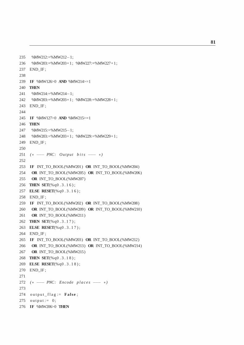
81
235 %MW212:=%MW212−1;
236 %MW203:=%MW203+1; %MW227:=%MW227+1;
237 END_IF ;
238
239 IF %MW126>0 AND %MW214>=1
240 THEN
241 %MW214:=%MW214−1;
242 %MW203:=%MW203+1; %MW228:=%MW228+1;
243 END_IF ;
244
245 IF %MW127>0 AND %MW215>=1
246 THEN
247 %MW215:=%MW215−1;
248 %MW203:=%MW203+1; %MW229:=%MW229+1;
249 END_IF ;
250
251 (∗ −−− PNC: Output b i t s−−− ∗ )
252
253 IF INT_TO_BOOL(%MW201) OR INT_TO_BOOL(%MW204)
254 OR INT_TO_BOOL(%MW205) OR INT_TO_BOOL(%MW206)
255 OR INT_TO_BOOL(%MW207)
256 THEN SET(%q0 . 3 . 1 6 ) ;
257 ELSE RESET(%q0 . 3 . 1 6 ) ;
258 END_IF ;
259 IF INT_TO_BOOL(%MW202) OR INT_TO_BOOL(%MW208)
260 OR INT_TO_BOOL(%MW209) OR INT_TO_BOOL(%MW210)
261 OR INT_TO_BOOL(%MW211)
262 THEN SET(%q0 . 3 . 1 7 ) ;
263 ELSE RESET(%q0 . 3 . 1 7 ) ;
264 END_IF ;
265 IF INT_TO_BOOL(%MW203) OR INT_TO_BOOL(%MW212)
266 OR INT_TO_BOOL(%MW213) OR INT_TO_BOOL(%MW214)
267 OR INT_TO_BOOL(%MW215)
268 THEN SET(%q0 . 3 . 1 8 ) ;
269 ELSE RESET(%q0 . 3 . 1 8 ) ;
270 END_IF ;
271
272 (∗ −−− PNC: Encode p l a c e s−−− ∗ )
273
274 o u t p u t _ f l a g := Fa lse;
275 o u t p u t := 0 ;
276 IF %MW206>0 THEN

82 PLC Program
277 IF o u t p u t _ f l a g THEN o u t p u t : = 1 5 ;
278 ELSE o u t p u t : = 1 ; o u t p u t _ f l a g :=True ;
279 END_IF ;
280 END_IF ;
281 IF %MW209>0 THEN
282 IF o u t p u t _ f l a g THEN o u t p u t : = 1 5 ;
283 ELSE o u t p u t : = 2 ; o u t p u t _ f l a g :=True ;
284 END_IF ;
285 END_IF ;
286 IF %MW213>0 THEN
287 IF o u t p u t _ f l a g THEN o u t p u t : = 1 5 ;
288 ELSE o u t p u t : = 3 ; o u t p u t _ f l a g :=True ;
289 END_IF ;
290 END_IF ;
291 IF %MW207>0 THEN
292 IF o u t p u t _ f l a g THEN o u t p u t : = 1 5 ;
293 ELSE o u t p u t : = 4 ; o u t p u t _ f l a g :=True ;
294 END_IF ;
295 END_IF ;
296 IF %MW208>0 THEN
297 IF o u t p u t _ f l a g THEN o u t p u t : = 1 5 ;
298 ELSE o u t p u t : = 5 ; o u t p u t _ f l a g :=True ;
299 END_IF ;
300 END_IF ;
301 IF %MW212>0 THEN
302 IF o u t p u t _ f l a g THEN o u t p u t : = 1 5 ;
303 ELSE o u t p u t : = 6 ; o u t p u t _ f l a g :=True ;
304 END_IF ;
305 END_IF ;
306 IF %MW205>0 THEN
307 IF o u t p u t _ f l a g THEN o u t p u t : = 1 5 ;
308 ELSE o u t p u t : = 7 ; o u t p u t _ f l a g :=True ;
309 END_IF ;
310 END_IF ;
311 IF %MW210>0 THEN
312 IF o u t p u t _ f l a g THEN o u t p u t : = 1 5 ;
313 ELSE o u t p u t : = 8 ; o u t p u t _ f l a g :=True ;
314 END_IF ;
315 END_IF ;
316 IF %MW214>0 THEN
317 IF o u t p u t _ f l a g THEN o u t p u t : = 1 5 ;
318 ELSE o u t p u t : = 9 ; o u t p u t _ f l a g :=True ;

83
319 END_IF ;
320 END_IF ;
321 IF %MW204>0 THEN
322 IF o u t p u t _ f l a g THEN o u t p u t : = 1 5 ;
323 ELSE o u t p u t : = 1 0 ; o u t p u t _ f l a g :=True ;
324 END_IF ;
325 END_IF ;
326 IF %MW211>0 THEN
327 IF o u t p u t _ f l a g THEN o u t p u t : = 1 5 ;
328 ELSE o u t p u t : = 1 1 ; o u t p u t _ f l a g :=True ;
329 END_IF ;
330 END_IF ;
331 IF %MW215>0 THEN
332 IF o u t p u t _ f l a g THEN o u t p u t : = 1 5 ;
333 ELSE o u t p u t : = 1 2 ; o u t p u t _ f l a g :=True ;
334 END_IF ;
335 END_IF ;
336 IF %MW217>0 THEN
337 IF o u t p u t _ f l a g THEN o u t p u t : = 1 5 ;
338 ELSE o u t p u t : = 1 5 ; o u t p u t _ f l a g :=True ;
339 END_IF ;
340 END_IF ;
341 %q0 . 3 . 2 4 := ( o u t p u t & 1 ) < >0;
342 %q0 . 3 . 2 5 := ( o u t p u t & 2 ) < >0;
343 %q0 . 3 . 2 6 := ( o u t p u t & 4 ) < >0;
344 %q0 . 3 . 2 7 := ( o u t p u t & 8 ) < >0;

84 PLC Program

Appendix D
Arduino program
The Arduino main program functions are listed in this appendix. The program way of working
and functions are explain in section 3.4.1.
1
2 i n t s e r i a l _ r e a d _ s t r (char ∗buf , i n t b u f l e n ) {
3 / / read t i l l t h e end o f t h e b u f f e r or a t e r m i n a t i n g char
4 i n t i , c ;
5 i f ( S e r i a l . a v a i l a b l e ( ) <= 0) {
6 re turn 0 ;
7 }
8 f o r ( i =0; i < bu f l en−1; i ++) {
9 c= S e r i a l . r ead ( ) ;
10 i f ( c==0 | | c==0x0A ) break ;
11 ∗buf ++= c ;
12 i f ( S e r i a l . a v a i l a b l e ( ) <= 0) {
13 de l ay ( 1 0 ) ; / / 10 m i l l i s e c o n d s = 96 b i t s / 9600 b i t s / sec
14 i f ( S e r i a l . a v a i l a b l e ( ) <= 0)break ;
15 }
16 }
17 ∗buf= ’ \ 0 ’ ;
18 re turn 1 ;
19 }
20
21 void main_send_end_cmd ( ) {
22 S e r i a l . p r i n t l n ( "> " ) ;
23 }
24
25 void s t o r e _ i n p u t s ( ) {
26 boo l change = f a l s e ;

86 Arduino program
27 f o r ( by te i = 0 ; i < IN_PINS ; i ++) {
28 boo l l a s t S t a t e = b i tRead ( l a s t R e a d i n g , i ) ;
29 boo l p i n S t a t e ;
30 p i n S t a t e = d i g i t a l R e a d ( i _ p i n s [ i ] ) ;
31 t ime = m i l l i s ( ) ;
32 i f ( p i n S t a t e != l a s t S t a t e ) {
33 change = t r u e ;
34 b i t W r i t e ( l a s t R e a d i n g , i , p i n S t a t e ) ;
35 }
36 }
37 / / i f change i s t r u e a t l e a s t one p in s t a t e changed
38 / / and l a s t R e a d i n g w i l l c o n t a i n p i n s s t a t e s
39 i f ( change ) {
40 d a t a [ chgs ] = l a s t R e a d i n g ;
41 t i m e _ d a t a [ chgs ] = t ime− t i m e _ i n i ;
42 chgs ++;
43 }
44 }
45
46 void t f i r e ( ) {
47 t ime = t ime − t i m e _ i n i ;
48 t ime = t ime / 1 0 0 0 ;
49 i f ( p l c _ i n i t == f a l s e ) {
50 d i g i t a l W r i t e ( o_p ins [ 7 ] , t r u e ) ;
51 de layM ic roseconds ( 1 0 0 0 ) ;
52 d i g i t a l W r i t e ( o_p ins [ 7 ] , f a l s e ) ;
53 p l c _ i n i t = t r u e ;
54 }
55 i f ( t ime > 20) {
56 r e c o r d = f a l s e ;
57 f i r e = f a l s e ;
58 r e c o r d _ i n i = f a l s e ;
59 p l c _ i n i t = f a l s e ;
60 f o r ( i n t i =0 ; i <= 3 ; i ++) { d i g i t a l W r i t e ( o_p ins [ i ] , f a l s e ) ; }
61 main_send_end_cmd ( ) ;
62 }
63 / / Sends d e f i n e d key s i g n a l depend ing on t ime s i n c e t f i r e ( ) has began .
64 e l s e { k e y s _ p r e s s e d _ a t _ t i m e ( ) ; }
65 }

Bibliography
[1] Christos G. Cassandras and Stéphane Lafortune.Introduction to discrete event systems.
Springer Science+Business Media, New York, N.Y, 2008.
[2] Steven J. Cunning and Jerzy W. Rozenblit. Automating test generation for discrete event
oriented embedded systems.Journal of Intelligent and Robotic Systems, 41(2-3):87–112,
2005.
[3] Geoff Cutts and Shaun Rattigan. Using Petri nets to developprograms for PLC systems.
In Application and Theory of Petri Nets 1992, pages 368–372. Springer, 1992.
[4] Ana Paula Estrada-Vargas, Ernesto Lopez-Mellado, and Jean-Jacques Lesage. Automated
modelling of reactive discrete event systems from externalbehavioural data. InElectron-
ics, Communications and Computing (CONIELECOMP), 2013 International Conference
on, pages 120–125. IEEE, 2013.
[5] Ana Paula Estrada-Vargas, Ernesto Lopez-Mellado, and Jean-Jacques Lesage. Identifica-
tion of partially observable discrete event manufacturingsystems. InEmerging Technolo-
gies & Factory Automation (ETFA), 2013 IEEE 18th Conference on, pages 1–7. IEEE,
2013.
[6] Eurocircuits. Online pcb prototype and small series specialist.
http://www.eurocircuits.com/, 2015.
[7] A. Gordon, F. Bousseau, and N. Dangoumau. PM Editor.
[8] Tao Huang and Anthony Chung. Communication networks and systems in substations.
2004.
[9] M. V. Iordache and P. J. Antsaklis. Supervision Based on Place Invariants: A Survey.
Discrete Event Dynamic Systems, 16(4):451–492, December 2006.

88 BIBLIOGRAPHY
[10] Marian V. Iordache and Panos J. Antsaklis. Software tools for the supervisory control of
Petri nets based on place invariants.ISIS, page 003, 2002.
[11] Marian V. Iordache and Panos J. Antsaklis. Synthesis ofsupervisors enforcing firing vector
constraints in petri nets.ISIS, page 002, 2002.
[12] Marian V. Iordache and Panos J. Antsaklis. Decentralized control of Petri nets with con-
straint transformations. InAmerican Control Conference, 2003. Proceedings of the 2003,
volume 1, pages 314–319. IEEE, 2003.
[13] Marian Valentin. Iordache and Panos J. Antsaklis.Supervisory control of concurrent sys-
tems a Petri net structural approach. Birkhäuser, Boston, 2004.
[14] S. Jain, R. R. Creasey, J. Himmelspach, K. P. White, and M. Fu.VERIFICATION AND
VALIDATION OF SIMULATION MODELS.
[15] Thomas Mertke and Georg Frey. Formal Verification Of PLC-Progams Generated From
Signal Interpreted Petri Nets. InIEEE Systems, Man, and Cybernetics Conference. IEEE,
2001.
[16] Mark Minas and Georg Frey. Visual PLC-Programming usingSignal Interpreted Petri
Nets. InAmerican Control Conference, 2003, 2002.
[17] John O. Moody and Panos J. Antsaklis.Supervisory Theory of DES Using Petri Nets.
Kluwer Academic Publishers, Notre Dame, 1998.
[18] Thomas H. Naylor, J. M. Finger, James L. McKenney, William E. Schrank, and Charles C.
Holt. Verification of computer simulation models.Management Science, 14(2):pp. B92–
B106, 1967.
[19] Paulo Oliveira. Industrial processes automation (course IST/MEEC). https:
//fenix.tecnico.ulisboa.pt /disciplinas /APInd /2010-2011 /1-semestre, 2010.
[20] Fernando Pereira and Luís Gomes. Automatic synthesis of VHDL Hardware Components
from IOPT Petri Net models. InIEEE, 2013.
[21] James L. Peterson.Petri Net Theory and the Modeling of Systems. Pretice-Hall, Austin,
Texas, 1981.
[22] Carl Petri.Communication With Automata. PhD thesis, Darmstadt University of Technol-
ogy, 1962.
BIBLIOGRAPHY 89
[23] Jean-Marc Roussel and Jean-Jacques Lesage. Validationand verification of grafcets using
state machine. InIMACS-IEEE" CESA’96", pages pp–758, 1996.
[24] Klein S, Georg Frey, and Mark Minas. PLC Programming with Signal Interpreted Petri
Nets. InICATPN, LNCS, 2003.
[25] S. Schlesinger.Terminology for model credibility. 1979.
[26] Tamas Schne and Tibor Holczinger. Coloured Petri Net based PLC program validation
with a fast simulation method. InProcess Control (PC), 2013 International Conference
on, pages 179–184. IEEE, 2013.
[27] Martina Svádová and Zdenek Hanzálek. Matlab toolbox for petri nets. In22nd Interna-
tional conference ICATPN 2001, pages 32–36, 2001.