monografies de l’institut d’investigacio en intel lig ... · iiia, institut d’investigaci o...
TRANSCRIPT

MONOGRAFIES DE L’INSTITUT D’INVESTIGACIO
EN INTEL·LIGENCIA ARTIFICIAL
Number 1
Institut d’Investigacioen Intel·ligencia Artificial
Monografies de l’Institut d’Investigacio en
Intel·ligencia Artificial
Num. 1 J. Puyol, MILORD II: A Language for Knowledge–BasedSystems
Num. 2 J. Levy, The Calculus of Refinements, a Formal SpecificationModel Based on Inclusions
Num. 3 Ll. Vila, On Temporal Representation and Reasoning inKnowledge–Based Systems
Num. 4 M. Domingo, An Expert System Architecture for Identificationin Biology

MILORD II: A Language for
Knowledge–Based Systems
Josep Puyol i Gruart
Foreword by Jaume Agustı
Institut d’Investigacio en Intel·ligencia Artificial
Bellaterra, Catalonia, Spain.

Series EditorInstitut d’Investigacio en Intel·ligencia ArtificialConsell Superior d’Investigacions Cientıfiques
Foreword byJaume AgustıInstitut d’Investigacio en Intel·ligencia ArtificialConsell Superior d’Investigacions Cientıfiques
Volume AuthorJosep Puyol i GruartInstitut d’Investigacio en Intel·ligencia ArtificialConsell Superior d’Investigacions Cientıfiques
Institut d’Investigacioen Intel·ligencia Artificial
ISBN: 84–00–07499–8ISSN: 1135–4100Dep. Legal: B–34740–95c© 1995 by Josep Puyol i Gruart
All rights reserved. No part of this book may be reproduced in any form or byany electronic or mechanical means (including photocopying, recording, or infor-mation storage and retrieval) without permission in writing from the publisher.Ordering Information: Text orders should be addressed to the Library of theIIIA, Institut d’Investigacio en Intel·ligencia Artificial, Campus de la UniversitatAutonoma de Barcelona, 08193 Bellaterra, Barcelona, Spain.
Printed by Cardellach Copies, S.L. CBS, S.A.
Sant Pere, 40.
08221 Terrassa, Spain.

Als meus pares.A Carme i Pau.


Contents
Foreword xi
Preface xiii
Abstract xv
1 Introduction 11.1 Motivation . . . . . . . . . . . . . . . . . . . . . . . . . . . . . . 1
1.1.1 Real World Expert Systems . . . . . . . . . . . . . . . . . 11.2 From Milord to Milord II . . . . . . . . . . . . . . . . . . . . . 3
1.2.1 Milord Characteristics . . . . . . . . . . . . . . . . . . . . 31.2.2 Differences and Improvements . . . . . . . . . . . . . . . . 4
1.3 Related Work . . . . . . . . . . . . . . . . . . . . . . . . . . . . . 61.3.1 Purpose . . . . . . . . . . . . . . . . . . . . . . . . . . . . 71.3.2 Modularity . . . . . . . . . . . . . . . . . . . . . . . . . . 71.3.3 Approximate Reasoning . . . . . . . . . . . . . . . . . . . 81.3.4 Inference Engines . . . . . . . . . . . . . . . . . . . . . . . 91.3.5 Control . . . . . . . . . . . . . . . . . . . . . . . . . . . . 10
1.4 Main Contributions . . . . . . . . . . . . . . . . . . . . . . . . . . 101.5 Scheme of the Thesis . . . . . . . . . . . . . . . . . . . . . . . . . 13
2 Modularity 152.1 Introduction . . . . . . . . . . . . . . . . . . . . . . . . . . . . . . 16
2.1.1 Previous Work . . . . . . . . . . . . . . . . . . . . . . . . 172.1.2 Modular System . . . . . . . . . . . . . . . . . . . . . . . 17
2.2 Primitive Components . . . . . . . . . . . . . . . . . . . . . . . . 192.2.1 Interfaces of modules . . . . . . . . . . . . . . . . . . . . . 222.2.2 Modular hierarchy . . . . . . . . . . . . . . . . . . . . . . 242.2.3 Semantics of modules . . . . . . . . . . . . . . . . . . . . 25
2.3 Generic modules . . . . . . . . . . . . . . . . . . . . . . . . . . . 282.4 Refinement, Expansion and Contraction . . . . . . . . . . . . . . 32
2.4.1 Refinement . . . . . . . . . . . . . . . . . . . . . . . . . . 342.4.2 Expansion and Contraction . . . . . . . . . . . . . . . . . 40
2.5 Special declarations . . . . . . . . . . . . . . . . . . . . . . . . . 41
vii

2.5.1 Inherit and Open . . . . . . . . . . . . . . . . . . . . . . . 41
2.5.2 Sharing . . . . . . . . . . . . . . . . . . . . . . . . . . . . 43
2.5.3 Dynamic Modules . . . . . . . . . . . . . . . . . . . . . . 43
2.6 Conclusions . . . . . . . . . . . . . . . . . . . . . . . . . . . . . . 44
3 Approximate Reasoning 45
3.1 Algebra of truth–values . . . . . . . . . . . . . . . . . . . . . . . 47
3.1.1 Modus Ponens Operator . . . . . . . . . . . . . . . . . . . 50
3.2 Uncertainty and Imprecision . . . . . . . . . . . . . . . . . . . . . 51
3.2.1 Intervals of Truth–values . . . . . . . . . . . . . . . . . . 54
3.2.2 Working with intervals . . . . . . . . . . . . . . . . . . . . 56
3.2.3 Fuzzy Sets . . . . . . . . . . . . . . . . . . . . . . . . . . . 57
3.3 Local Logics . . . . . . . . . . . . . . . . . . . . . . . . . . . . . . 60
3.3.1 Mappings between different local logics . . . . . . . . . . 61
3.3.2 Example . . . . . . . . . . . . . . . . . . . . . . . . . . . . 63
3.4 Logic Declaration . . . . . . . . . . . . . . . . . . . . . . . . . . . 65
3.4.1 Truth values . . . . . . . . . . . . . . . . . . . . . . . . . 65
3.4.2 Connectives . . . . . . . . . . . . . . . . . . . . . . . . . . 66
3.4.3 Renaming . . . . . . . . . . . . . . . . . . . . . . . . . . . 67
3.5 Conclusions . . . . . . . . . . . . . . . . . . . . . . . . . . . . . . 68
4 Deduction by Specialization 71
4.1 Enriched Behavior . . . . . . . . . . . . . . . . . . . . . . . . . . 71
4.1.1 Communication . . . . . . . . . . . . . . . . . . . . . . . . 73
4.1.2 Solutions . . . . . . . . . . . . . . . . . . . . . . . . . . . 74
4.1.3 Validation . . . . . . . . . . . . . . . . . . . . . . . . . . . 79
4.1.4 Summary . . . . . . . . . . . . . . . . . . . . . . . . . . . 80
4.2 Specialization Calculus . . . . . . . . . . . . . . . . . . . . . . . . 81
4.2.1 Syntax . . . . . . . . . . . . . . . . . . . . . . . . . . . . . 81
4.2.2 Semantics . . . . . . . . . . . . . . . . . . . . . . . . . . . 82
4.2.3 Specialization Calculus . . . . . . . . . . . . . . . . . . . . 86
4.2.4 Soundness and Completeness . . . . . . . . . . . . . . . . 87
4.3 Implementation . . . . . . . . . . . . . . . . . . . . . . . . . . . . 87
4.3.1 Inference Engine Design . . . . . . . . . . . . . . . . . . . 88
4.3.2 Internal Representation of Deductive Knowledge . . . . . 89
4.3.3 Specialization . . . . . . . . . . . . . . . . . . . . . . . . . 90
4.4 The Deductive Knowledge Language . . . . . . . . . . . . . . . . 94
4.4.1 Facts . . . . . . . . . . . . . . . . . . . . . . . . . . . . . . 95
4.4.2 Rules . . . . . . . . . . . . . . . . . . . . . . . . . . . . . 100
4.4.3 Predicates on Facts . . . . . . . . . . . . . . . . . . . . . . 101
4.5 Conclusions . . . . . . . . . . . . . . . . . . . . . . . . . . . . . . 105
viii

5 Control 1075.1 Implicit Control . . . . . . . . . . . . . . . . . . . . . . . . . . . . 109
5.1.1 Subsumption . . . . . . . . . . . . . . . . . . . . . . . . . 1095.1.2 Unnecessary Rules . . . . . . . . . . . . . . . . . . . . . . 115
5.2 Threshold . . . . . . . . . . . . . . . . . . . . . . . . . . . . . . . 1165.3 Evaluation Strategy . . . . . . . . . . . . . . . . . . . . . . . . . 117
5.3.1 Lazy . . . . . . . . . . . . . . . . . . . . . . . . . . . . . . 1175.3.2 Eager . . . . . . . . . . . . . . . . . . . . . . . . . . . . . 119
5.4 Reification and Reflection Mechanisms . . . . . . . . . . . . . . . 1195.4.1 Static Reification . . . . . . . . . . . . . . . . . . . . . . . 1215.4.2 Dynamic Reification . . . . . . . . . . . . . . . . . . . . . 1225.4.3 Deductive Control . . . . . . . . . . . . . . . . . . . . . . 1245.4.4 Structural Control . . . . . . . . . . . . . . . . . . . . . . 124
5.5 Conclusions . . . . . . . . . . . . . . . . . . . . . . . . . . . . . . 126
6 Applications 1276.1 Introduction . . . . . . . . . . . . . . . . . . . . . . . . . . . . . . 1276.2 Terap-IA . . . . . . . . . . . . . . . . . . . . . . . . . . . . . . . . 128
6.2.1 Motivation and Goals . . . . . . . . . . . . . . . . . . . . 1286.2.2 Architecture . . . . . . . . . . . . . . . . . . . . . . . . . 1286.2.3 Implementation . . . . . . . . . . . . . . . . . . . . . . . . 131
6.3 Spong–IA . . . . . . . . . . . . . . . . . . . . . . . . . . . . . . . 1366.4 Ens–AI . . . . . . . . . . . . . . . . . . . . . . . . . . . . . . . . 1366.5 Fuzzy Control Example . . . . . . . . . . . . . . . . . . . . . . . 139
6.5.1 Simulation Process . . . . . . . . . . . . . . . . . . . . . . 1406.5.2 Controller . . . . . . . . . . . . . . . . . . . . . . . . . . . 1416.5.3 Results . . . . . . . . . . . . . . . . . . . . . . . . . . . . 145
6.6 Propagation Rules for Polytrees . . . . . . . . . . . . . . . . . . . 1466.6.1 Introduction . . . . . . . . . . . . . . . . . . . . . . . . . 1466.6.2 Implementation over Milord II . . . . . . . . . . . . . . 150
6.7 Future Applications . . . . . . . . . . . . . . . . . . . . . . . . . 1556.8 Conclusions . . . . . . . . . . . . . . . . . . . . . . . . . . . . . . 155
7 Conclusions 1577.1 Future Work . . . . . . . . . . . . . . . . . . . . . . . . . . . . . 158
A Syntax of Milord II 161A.1 Notation . . . . . . . . . . . . . . . . . . . . . . . . . . . . . . . . 161A.2 Modular System . . . . . . . . . . . . . . . . . . . . . . . . . . . 163A.3 Deductive Knowledge . . . . . . . . . . . . . . . . . . . . . . . . 164
A.3.1 Dictionary . . . . . . . . . . . . . . . . . . . . . . . . . . . 164A.3.2 Rules . . . . . . . . . . . . . . . . . . . . . . . . . . . . . 164
A.4 Inference System . . . . . . . . . . . . . . . . . . . . . . . . . . . 166A.5 Control Knowledge . . . . . . . . . . . . . . . . . . . . . . . . . . 167
A.5.1 Evaluation Type . . . . . . . . . . . . . . . . . . . . . . . 167A.5.2 Truth Threshold . . . . . . . . . . . . . . . . . . . . . . . 167
ix

A.5.3 Deductive Control . . . . . . . . . . . . . . . . . . . . . . 167A.5.4 Structural Control . . . . . . . . . . . . . . . . . . . . . . 167
B Proofs 169B.1 Proposition . . . . . . . . . . . . . . . . . . . . . . . . . . . . . . 169B.2 Soundness Theorem . . . . . . . . . . . . . . . . . . . . . . . . . 171B.3 Restricted Completeness . . . . . . . . . . . . . . . . . . . . . . . 171
B.3.1 Literal Completeness . . . . . . . . . . . . . . . . . . . . . 171B.3.2 Restricted Literal Completeness Theorem . . . . . . . . . 174
C Code Examples 177C.1 Terap–IA Example . . . . . . . . . . . . . . . . . . . . . . . . . . 177C.2 Fuzzy Control Example . . . . . . . . . . . . . . . . . . . . . . . 195
C.2.1 Controller . . . . . . . . . . . . . . . . . . . . . . . . . . . 196C.2.2 Simulator . . . . . . . . . . . . . . . . . . . . . . . . . . . 202C.2.3 Whole Process . . . . . . . . . . . . . . . . . . . . . . . . 202
C.3 Polytrees Example . . . . . . . . . . . . . . . . . . . . . . . . . . 204
List of Figures 209
List of Tables 211
References 213
Index 221
x

Foreword
The Expert System Shell presented in this book, Milord II, is the result ofa long and intensive research effort made during eight years within the IIIA
in developing several real life Expert Systems. Milord II has been designedand implemented not only having some possible usages in mind, but duringand through the applications development. To obtain the computational toolsthat do some tasks previously done by professionals. So Milord II although itgeneralizes from the particular domains who guided its design – mainly medicine– it should be best understood and be most useful for the generic tasks it wasthought for, classification problem solving. This specialization, the narrow anddeep adaptation to a kind of problem, I think is a mark of good engineering.Practical engineering including software engineering should be domain driven.
The author of the book fits perfectly well into this dynamic pattern of prac-tical, day to day engineering. The practical solutions he gave to the problemswere frequently ahead of the theoretical reflection and the foundational effort.Because the book is the Ph.D. Thesis of the author this practical trend is madeless evident than it could be. Only the last chapter on applications is completelydevoted to show it. The four central chapters of the book show the theoreticaland technical foundations of Milord II. Firmly grounded on them, Milord IIis a powerful tool for classification problem solving with uncertain and incom-plete information, allowing modular and incremental development and reuse ofsolutions.
Bellaterra, February 1996Jaume Agustı
Head of theFormal Methods Department
of the IIIA, CSIC
xi

xii

Preface
One of the main topics at the IIIA has been the study and development ofKnowledge–Based Systems, going from the theoretical aspects to the practicaldevelopment of languages for Expert Systems and real world applications.
Since 1985 our group has been working on the development of a shell forExpert System named Milord. The first version of Milord was finished in 1989.Milord introduced great important advances on uncertainty management lan-guages and multi–level architectures for Expert Systems. The main applicationsdeveloped using Milord were in the medical domain. The most important wasPneumon–IA, an Expert System for the diagnosis of pneumoniae.
The acceptance of Milord shell and its applications prompted us to think ina second version much renewed of the shell we named Milord II. Since 1989 wehave been developing Milord II, which is the topic of the present work.
As it can be seen from the structure of this book the new contributionshave been the modularization, the uncertainty management, the deduction byspecialization and the reflective control architecture of Milord II. Like in Mi-
lord, this research has been driven by the applications, then a set of new realworld applications and examples have been developed using Milord II. In thisbook we present some Expert Systems on different domains: Spong–IA, foridentification of marine sponges; Terap–IA, for treatment of pneumoniae (thenatural extension of Pneumon–IA); Ens–AI, for psicopedagogical diagnosis; andsome small examples.
The research on Milord II is not considered to be finished in the sense thatnew applications and ideas still contribute to the continuous enrichement of thelanguage. Now we are working on a new version of Milord II (MilordAgents?) based on Multi–Agent Systems. The main idea is to study the cooperationof cognitive agents based on Milord II modules.
Milord II has been developed in Common Lisp (the interpreter) and inC (the compiler). This software is available for research and educational pur-poses. A fresh version for Macintosh1 machines can be obtained by anonymousftp at ftp.iiia.csic.es in the directory /pub/Milord/mac, or in the WWW athttp://www.iiia.csic.es/˜puyol. Now we are working on versions for PC andUnix machines.
1Macintosh is a trademark of Apple Computer, Inc.
xiii

Acknowledgments
This work has been influenced by many people. I specially thank Jaume Agustı,who introduced me to research activities and who has provided guidance andsupport in the development of this work.
Carlos Sierra has greatly influenced this work because this thesis is the nat-ural extension of his previous work, Milord. He has provided me extensivesupport. We had large discussions on Milord II and I have benefited of hisadvice and assistance during Milord II design and application development.
Lluıs Godo has collaborated in all the questions dealing with uncertaintymanagement.
I am in debt with the experts that have applied Milord II to real worldproblems. Pilar Barrufet, Marta Domingo, Clara Barroso and Lluıs Murguihave been patient and constant users of my system.
The Milord II Compiler has been developed by Josep Lluıs Arcos. He hassuffered all the continuous changes we were introducing in the language.
Finally I would thank all the IIIA colleagues and friends for their collabora-tion and support, specially Francesc Esteva, IIIA Director, and Ramon Lopezde Mantaras, head of our group.
All this work has been developed first in the Artificial Intelligence Group atthe Center for Advanced Studies of Blanes (CEAB), which in October 1995moved to the newly created Artificial Intelligence Research Institute (IIIA).CEAB and IIIA are research institutes from the Spanish Scientific ResearchCouncil (CSIC). This work has been financed mainly by CICYT Spanish projects,SPES project n. 880j382 and TESEU project TIC91–0430. My thanks to theseInstitutions for providing the necessary means for the development of this work.
Bellaterra, February 1996Josep Puyol i Gruart
E–mail: [email protected]://www.iiia.csic.es/˜puyol
xiv

Abstract
Milord II is an architecture and a language for the development of knowledge–based systems. In particular we are interested in real world Expert Systems, thatis, those that are useful in a real environment and that have real purposes. Todo that we propose a language based on modules as a method for programmingin the large. Modules, generic modules and a set of operations on them are thebasis of this language. A program in Milord II is then a hierarchical structureof modules. A module is an encapsulated unit with a well defined interface toother modules. Each module is composed of deductive knowledge (weighted factsand rules), local logic (a truth values algebra declaration) and a local controlcomponent (Horn–like metarules).
Each module contains its own local logic to deal with approximate reasoning.An algebra of truth–values is defined to perform the deductions in a weightedrule–based language (deductive knowledge). A mechanism is provided to findvalid translations of the terms communicated between modules with differentlogics.
The deduction mechanism of Milord II is based on the concept of Spe-cialization. This leads to a new inference engine which improves the deductioncompared with the engines based on Modus ponens. These improvements facili-tates the communication with the user, the validation and the understanding ofExperts Systems.
Finally we discuss a set of applications and examples developed using Mi-lord II.
xv

xvi

Chapter 1
Introduction
To introduce the content of this thesis it is necessary first to talk about what arethe problems we want to handle, and what is the kind of solutions we propose.Here it is very important to fix the type of problems, its environment, what kindof solutions we are interested in, where, and who is the user of those solutions.In this Chapter the motivation, the history and a summed up description ofMilord II modular language and its environment are presented.
1.1 Motivation
We say that somebody is an expert when he is skilled in some matter by practice.Examples of human experts are physicians, biologists, mechanics, engineers, andso on. They are able to solve problems by using knowledge obtained by practice,despite they also have somewhat deep knowledge about their knowledge domain.Expert Systems (ESs) have proved to be useful tools to automate this kind ofproblem solving.
The goal of this thesis has been the design and implementation of a modularlanguage named Milord II, that offers a powerful, simple and friendly environ-ment to develop ESs. We should notice that the starting point of this thesis wasthe previous language Milord. This language and their applications allowed usto experience new problems, which guided us to the design of a new languagebased on the previous one.
First we should fix what kind of Expert Systems Milord II is intendedfor, and who are the expected programmers and users of Milord II and itsapplications.
1.1.1 Real World Expert Systems
One of the main characteristics of Milord II is that it addresses the developmentof real world ESs, that is, the problems we want to solve are not toy examples,
1

2 Chapter 1. Introduction
and both the programmers and the users are professionals interested in obtaininggood results from the system.
Below we present the main characteristics of our work environment, that leadus to the actual design and implementation of Milord II.
• We think that the programmers of ES applications with Milord II areexperts in some knowledge domain. Normally they are not knowledgeengineers or artificial intelligence specialists. In general, they deal withapplication domains where expertise is required, for instance medical orbiological domains. That means that they need simple tools and simplelanguages to develop their applications1. Milord II has been designed tobe an easy to use system.
• Experts are qualified and busy professionals, then we should offer friendlytools to them. Simplifications of problems would lead us to good examples,but the interest of experts in them will be poor. This implies the need tohandle non simplified real problems to motivate the use of the system byexperts. In this case programming an ES becomes a useful work beingable to structure, understand and diffuse the own knowledge the experthas. Experts have used Milord II to develop ES applications as biologicalclassification, medical diagnosis, etc.
• Notice that our applications are highly interactive and that this interactionis done with humans. We consider users of Milord II people who workswith the ESs generated by programmers. Users have different levels ofexpertise. They can be experts in the domain knowledge of the system, ornon expert users. It both cases they need a good communication with thesystem and a high level of confidence on it. Specialization is a key conceptintroduced in Milord II to produce a good communication with the users.
• Some features of the real applications are the big size, and the incomplete,imprecise and uncertain knowledge they have. To match these character-istics we needs an expressive language that provides structuration tools,incremental design, reutilization of components and approximate reason-ing. These characteristics are very important in the design of Milord II.Modularity and uncertainty treatment are the key points of the systemtogether with specialization.
• Most of the problems we want to handle are classification tasks. We con-sider classification the task of finding solutions in a known and finite searchspace. Milord has been applied mostly to this kind of applications, andMilord II follows the same way. Examples of classification applicationsare medical diagnosis, biological classification, and so on.
1Considering the experts as programmers do not mean that applications are totally devel-oped by experts. In our case experts have continuous advising from us, we take then the roleof knowledge engineer. It is easy to see that if experts have a good knowledge of the tools theyare using, the communication between the expert and the knowledge engineer is easier.

1.2. From Milord to Milord II 3
• Finally we think that real applications should work in real environments.The lack of informatic resources in the environments where the applica-tions could be tested and used is a common problem. This contributes toisolate the system. We should accommodate and we did it the resourcerequirements and the efficiency of Milord II shell to the most normalmachines usually present in the environment of the application.
We have explained the main features and problems that experts and users2
of Real ESs must face. In this thesis we will propose solutions for that. Atthis point we should talk about the previous experience with Milord and theimprovements that Milord II introduces to handle the kind of ESs describedabove.
1.2 From Milord to Milord II
Notice that the development of Milord II was possible thanks to our previousexperience acquired in ES design. The acceptance of Milord Shell (Godo etal., 1988; Sierra, 1989) and the applications developed allowed us to think in asecond version much renewed of the Shell we named Milord II. This experienceand all the considerations above lead us to the design and implementation ofMilord II Shell, keeping in mind that the programs should be useful in the realenvironment of the application domain.
The transition from Milord to Milord II was a natural one directed by theapplications. The main applications developed with Milord were in the medicalenvironment, as Pneumon–IA (diagnosis of pneumonia) (Verdaguer, 1989) andRENOIR (rheumatic disease diagnosis) (Belmonte, 1991). Furthermore Milord
was the starting point of new works on validation (Meseguer, 1992) and case–based reasoning (Lopez, 1993).
The new applications we are developing with Milord II are: Pneumon–
IA II (a modular version of Pneumon–IA, a system for pneumonia diagnosis),Terap–IA (treatment of pneumonia), Spong–IA (sponge classification) and Ens–
AI (psycho–pedagogical diagnosis).To see the improvements and differences of Milord II with respect to the
previous version we summarize Milord characteristics in the following. The needsdetected during the development of the applications have guided the improve-ments of the system.
1.2.1 Milord Characteristics
It is not our purpose here to describe exhaustively the Milord system. Here wewant to point out those elements that had a close relation to the new design.We can summarize the main characteristics of Milord in the following points:
2Notice that in the following, when there is no ambiguity, we will use experts meaning theprogrammers of Milord II applications. When it is necessary we will distinguish betweenusers and expert users.
4 Chapter 1. Introduction
Multi–level Architecture: One of the main purpose of Milord was the clearseparation among different sorts of knowledge, that is, associative, struc-tural, hypothetic and heuristic. That architecture allowed the experts togive a good structuration of his knowledge providing a clear separationbetween domain and control knowledge.
Uncertainty Treatment: A good effort was done to approach and representthe type of uncertainty the experts normally use to express their knowl-edge. Milord used fuzzy logic with linguistic labels to represent uncertainty.Experts were able to define their own logic in the applications.
Modularity: A first proposal (design not implementation) of modularity wasdone in Milord in order to support programming in the large. This proposalwas based in the modularization of the domain knowledge only as a staticstructuration tool. Before the interpretation of a program, it had to becompiled to a flat structure, that is, to an equivalent and non modularprogram. The multilevel architecture of control was outside this modularstructuration.
Communication: The behavior of Milord was the standard of many ExpertSystems. The user gives a goal to the ES, and the ES asks to the user forthe values of the facts which are relevant to obtain a solution. Finally theES answers the value of the goal, or unknown if it was not able to obtaina solution.
Implementation: The version of flat3 Milord was implemented and tested withthe applications mentioned above. Because of the great amount of re-sources that symbolic computation consumes (Milord was programmed inCommon Lisp), the current technological state forced the use of mini com-puters to implement and run Milord.
Following the above points we can give a brief analysis of the main differencesand improvements of Milord II with respect to Milord.
1.2.2 Differences and Improvements
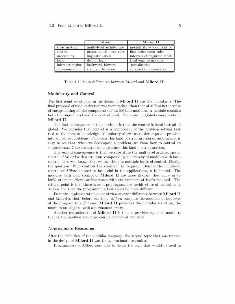
Milord and Milord II have many common points, going from the characteristicsof the language to the applications programmed with them. It is very difficultto analyze in depth these points without making an exhaustive explanation ofboth systems. For that reason here we only describe the main conceptual andarchitectural differences between Milord and Milord II leaving the details of thecommon points and the differences to be explained along this thesis. The pointswe will take into account are: modularity, approximate reasoning, behavior andcommunication. A summary of these differences between Milord and Milord IIare given in the Table 1.1.
3Modular Milord was not implemented.
1.2. From Milord to Milord II 5
Milord Milord II
structuration multi–level architecture modularity + local control
control propositional meta–rules first–order meta–rules
uncertainty linguistic labels intervals of linguistic labels
logic default logic local logic to modules
inference engine backward, forward specialization
communication standard behavior enriched communication
Table 1.1: Main differences between Milord and Milord II.
Modularity and Control
The first point we studied in the design of Milord II was the modularity. Thefinal proposal of modularization was more radical than that of Milord in the senseof encapsulating all the components of an ES into modules. A module containsboth the object level and the control level. There are no global components inMilord II.
The first consequence of that decision is that the control is local instead ofglobal. We consider that control is a component of the problem solving tasktied to the domain knowledge. Modularity allows us to decompose a probleminto simple subproblems. Following this kind of structuration of problems, it iseasy to see that, when we decompose a problem, we know how to control itssubproblems. Global control would confuse this kind of structuration.
The second consequence is that we substitute the multilevel architecture ofcontrol of Milord with a structure composed by a hierarchy of modules with localcontrol. It is well known that we can think in multiple levels of control. Finallythe question ”Who controls the control?” is frequent. Despite the multilevelcontrol of Milord showed to be useful in the applications, it is limited. Themodules with local control of Milord II are more flexible, they allow us tobuild other multilevel architectures with the numbers of levels required. Thecritical point is that there is no a preprogrammed architecture of control as inMilord and then the programming task could be more difficult.
From the implementation point of view another difference between Milord IIand Milord is that, before run time, Milord compiles the modular object levelof the program to a flat one. Milord II preserves the modular structure, themodules are objects with a permanent entity.
Another characteristic of Milord II is that it provides dynamic modules,that is, the modular structure can be created at run time.
Approximate Reasoning
After the definition of the modular language, the second topic that was treatedin the design of Milord II was the approximate reasoning.
Programmers of Milord were able to define the logic that would be used in
6 Chapter 1. Introduction
their applications. Taking into account the modular structure of Milord II westudied the possibility of defining different logics into the different modules. Thismeans we can use different languages of representation in the different modules(Harper et al., 1989). Then, in Milord II the definition of logics is local to themodules and it provides mechanisms of communication between the differentlocal logics of the modules.
Another improvement of Milord II over the uncertainty treatment of Milord
is the introduction of imprecision. This is made by means of the extension ofthe uncertainty calculus of linguistics labels to the intervals of linguistics labels,and the use of fuzzy sets.
Behavior and Communication
One of the main goals of this thesis is to enrich the behavior of ESs. A standardES receives queries from the user, asks questions to the user, and finally answersthe queries of the user. We are interested in improving the way the system ask theuser, and in enriching the sort of answers the system gives to the user. Rememberthat normally our applications are interactive and the users are human. Thenthe following points are very important:
• It should be clear to the user that the sequence of questions he is answeringactually drives the system to the solution he is interested in, and that theinformation he gives to the system is properly used to find this solution.
• The solutions found by the system to the queries of the user should beinformative enough. For instance, the answer unknown is not informativeat all, it only says that the system was not able to find a solution.
To solve these problems Milord II introduces an inference engine based onspecialization of KBs. This kind of inference engine allows us to make indepen-dent the search and the deductive processes instead of the classical interleavedsearch and deductive processes of the standard inference engines as backwardand forward ones. This allows us to implement different control strategies in or-der to improve the quality of the process of obtaining information from the user.Furthermore the inference engine of Milord II is able to obtain conditionalanswers and deal with unknown answers from the user.
Finally notice that Milord II Shell runs over personal computers to facilitateits use by experts in the environment of the applications. This is not a merit ofthe implementation but of the new advances introduced in the current personalcomputers.
1.3 Related Work
After the first experiences with ESs at seventies (for instance, MYCIN (Short-liffe, 1976)) knowledge–based systems, and artificial intelligence in general, haveexperimented a continuous evolution of the ideas, styles and techniques.

1.3. Related Work 7
Artificial Intelligence have been more and more specialized and a great num-ber of new disciplines have come out. Knowledge representation, problem solvingmethods, approximate reasoning, methodologies for knowledge engineering, for-mal methods, learning, and so on, are examples of topics that have generated alot of work.
We will give a brief explanation of some aspects we consider they are the mostrelevant to relate with Milord II. The languages appeared in this Section arefrom the classical ones to other actual languages that we consider are interestingto be related with Milord II now, and in the future. You can find a veryinteresting description of some of these systems (including Milord II) througha common example in (Treur and Wetter, 1993). In the same book there is acomparison study of these languages (vanHarmelen et al., 1993).
1.3.1 Purpose
The first criteria for the comparison of languages is the purpose the languagespursue. We can distinguish between the languages that are designed to buildexecutable systems for some concrete applications from those that find formalspecifications of general tasks, problem solving methods, domain models and soon.
The purpose of the language determines the sort of development task used todesign and implement a concrete language for knowledge engineering. The lan-guages directed to the applications are designed following a bottom–up method-ology. There is a feedback cycle between the language designers and the expertswith their applications. Then, this kind of languages are incrementally designedand implemented on demands of the applications and the experts. The secondtype of languages are devoted to the modelization of more general problems andthey follow a top–down methodology of development.
The resultant languages designed with these approaches differ on their ex-presivity power. Those languages designed with the first type methodology aremore expressive and easy to use for the specific kind of problems they has beendesigned. The others can cope a wider set of problems, but the expresivity powerbecomes poor.
As explained in the introduction, we are interested in the implementation ofreal ESs, then the development of Milord II was directed by the applications itwas involved in. We have designed a language the more adapted to the kind ofproblems it is applied. AIDE (Greboval and Kassel, 1992) language has a similarapproach to develop real ESs and it is oriented to give good explanations. Mi-lord II is able to build real size applications.
1.3.2 Modularity
All the language designers agree with the need of providing programming con-structs for the modularization of the programs. Some languages encourage morethan others this technique and the architectures of the modular systems aredifferent.

8 Chapter 1. Introduction
In some cases the current methodologies for knowledge engineering, as com-ponents of expertise (Steels, 1990), KADS (Wielinga et al., 1992) or generictasks (Chandrasekaran, 1987), determine the kind of modularization used in thelanguages.
Several languages are related with KADS methodology such as (ML)2 (van-Harmelen and Balder, 1992), AIDE (Greboval and Kassel, 1992), KARL (Fensenet al., 1991), and KBSSF (Veld et al., 1993). These systems implement theglobal layering of KADS methodology, that is, domain, inference, task and strat-egy layers. The modularization is limited to be used into each layer, i.e. amodular structure in the task layer or in the strategic layer.
The language COMMET (Jonckers et al., 1992) uses the components of ex-pertise methodology based on tasks, models and methods.
Other languages as DESIRE (Langevelde et al., 1993) and the language MC(Giunchiglia et al., 1993) do not have this limitation and the specifications area set of interconnected reasoning modules, where each module is treated as anindependent unit. These languages are used to define different kind of modules,such as domain and control modules.
The approach of Milord II is different in the sense that each module containsthe domain knowledge (object level) and the local control knowledge (meta level)of the module. The interaction between modules is limited to object–object only,thus forcing purely local application of the meta–knowledge.
No one of the previous modularization techniques is based on the idea of amodule as a specialist like in Milord II.
Mostly of the languages (including Milord II) encourage the user to encapsu-late the local knowledge into modules. Other systems as AIDE has programmingconstructs but they do not force the user to exploit them. The modularizationtechniques of Milord II are based on theories used in the language ML (Harperet al., 1986).
1.3.3 Approximate Reasoning
Usually the information contained in the KBs is imperfect. Experts manageuncertain, imprecise, and incomplete information. Approximate reasoning isthen an important topic in the development of ESs.
There are three main approaches to deal with uncertainty, that is, the prob-abilistic, the evidential, and the possibilistic approach. Let us to give a briefvision of these approaches in order to situate that of Milord II.
There are several models based on probability. We can consider BayesianNetworks (Pearl, 1986), Nilsson’s Probabilistic Logic (Nilsson, 1986), SubjectiveBayesian Networks of PROSPECTOR (Duda et al., 1976), and Certainty Factorsof MYCIN (Shortliffe and Buchanan, 1975).
The lack of expressiveness is the main problem of the models based on prob-ability. They can not express vague predicates (for instance, tall). We mustspecify probabilities but in practice they represent subjective appreciations thatare not based on statistical analysis. In this case it is very difficult that ex-perts are able to represent these probabilities with enough precision by means

1.3. Related Work 9
of real numbers. Finally notice that the models based on bayesian networks arecomputationally expensive.
The evidential theory of Dempster–Shafer (Dempster, 1967; Shafer, 1976)has its main problem in the computational complexity, despite it is very usefulto manage uncertainty.
Both Milord and Milord II are based on possibilistic approaches. Zadehintroduced fuzzy logic to manage uncertainty and vagueness (Zadeh, 1975). Wethink that this approach provides an understandable and computationally effi-cient method to deal with imperfect information. Milord uses a linguistic approx-imation based on linguistic terms as fuzzy intervals (Godo et al., 1988; Sierra,1989). The expert declares the linguistic terms as fuzzy intervals by defininga trapezoidal characteristic function. From these declarations Milord computesthe truth tables of the conjunction, disjunction and implication operations. Inthe Milord approach still remains the problem of the numerical representationof the linguistic terms.
Milord II uses multi–valued propositional logic. The expert can choose aset of linguistic terms and define a set of logical operations directly on the setof linguistic values.
Milord II uses this kind of logic because multi–valued propositional sen-tences are easy to understand and to use for the kind of applications we arenormally involved. The lack of first order constructs is compensated by multi–valuedness of the logic (for instance, DESIRE use three–valued first order logic).
It is very important to notice that we extend the multi–valued logic to in-tervals of linguistic terms and that the modules of Milord II contain its ownlocal logic (Agustı et al., 1991; Agustı et al., 1992) . Milord II provides theconstructs of the language and a set of utilities to define different local logicsadapted to the different problems represented by different modules. Further-more we provide the method to find valid mappings between these logics inorder to communicate different modules with different local logics without lossof consistency.
1.3.4 Inference Engines
A lot of systems based on first order logic use the Prolog technology. In othercases the classical inference engines like that backward and forward ones areused. For instance, Teiresias (Davis, 1982) has simple control strategies basedon forward or backward engines.
As cited above the inference engine used in the modules of Milord II is basedon the specialization of KBs (Puyol, 1992a; Puyol et al., 1992b). Specializationis based on the notion of partial evaluation expressed in the well known Kleene’sTheorem (Kleene, 1952). Briefly, if we have a function of n arguments and weknow the value of an argument we can specialize this function obtaining a newone with the same arguments that before but the known one. We can consider aKB as a function with arguments the set of facts needed to reach the goal of theKB. We specialize the KB with a known fact obtaining a new KB specialized bythe new domain that contains the known fact.

10 Chapter 1. Introduction
Milord II is based on logic, then we use the term partial deduction instead ofpartial evaluation following the suggestion of Komorowski (Komorowski, 1981;Komorowski, 1990). Partial deduction algorithms have been intensively used inlogic programming (Venken, 1984; Gallagher, 1986; Komorowski, 1981; Takeuchiand Furukawa, 1986; Lloyd and Shepherson, 1991) mainly for efficiency purposes.Our approach is different for instance from the logic programming one usedin (Lloyd and Shepherson, 1991). There, partial evaluation was goal driven,whereas here partial evaluation is data driven.
Milord II inference engine is also related to other work on conditionedanswers (Demolombe, 1990; Vasey, 1986; Sakama and Itoh, 1986) and on thetreatment of unknown information (Wolstenholme, 1987). Specialization usedin Milord II allows us to obtain conditioned answers after the specialization ofa KB with the known information. Our system is able to answer a useful resulteven in the case of partially unknown information.
The main difference of Milord II specialization with respect to other usesof partial deduction, is that it is based on a multi–valued propositional languageand it is oriented to the improvement of the communication of ESs.
1.3.5 Control
The first type of production rule languages like OPS5 (Forgy, 1981) used to definea single level of production. Milord II as DESIRE have declarative controlthrough a reflection mechanism. Other systems use procedural, functional, orguided by the user control.
Milord II uses Horn–like rules to define the control knowledge of a module.Remember that the interaction between modules is limited to object–objectinteraction, then the meta–knowledge is local to each module (DESIRE and MChave metamodules).
Milord II does not use global control and all the components of control arelocal to the modules. This allows us to clarify the problem structuration givinga easy idea of the way control is implemented in an application.
1.4 Main Contributions
The main contribution of this thesis is the integration and implementation ofa set of techniques, like specialization in multi–valued logics, and theoreticalresults, some of them introduced here, into a language for the development ofESs. The language has been implemented and a set of real size applications hasbeen developed.
The structure of this thesis is aimed at a deep, exhaustive and understandabledescription of the Milord II system. Then we summarize the contributions ofthe thesis following the same scheme of the thesis Chapter by Chapter.
Chapter 2. A modular language which allows a top–down and incrementalmethodology of ESs programming.

1.4. Main Contributions 11
Classical software engineering approves top–down design as a good pro-gramming methodology. The modular language of Milord II allows ex-perts to develop programs with a disciplinated methodology based on thedecomposition of problems into simpler subproblems.
Each module of Milord II contains all the components that usually definea whole ES, that is, the domain knowledge, the control knowledge, the logicand so on. The idea of a module as a local expert or specialist distinguishesour modular system from others. Then we can consider an ES as composedof a set of ESs modules, one for each subproblem to solve. Modules areorganized into a hierarchical structure that provide the form of integratingthe solutions of the subproblems to build the solution of the whole problem.
Incremental programming is another interesting feature of top–down pro-gramming. It consists in defining problems at different level of detail,initially by means of a partial description which is successively refined ob-taining more concrete definitions of the problem. We stop when the levelof detail is the required one.
The modules have a well defined interface, and the language also providesgeneric modules and a set of operations devoted to the incremental pro-gramming of modules.
The contributions of this Chapter to the development methodology ofknowledge–based systems are the following:
• A methodology of programming based on problem decomposition.
• An homogeneous language based on modules, generic modules andoperations between them. The primitive component of Milord II arethe modules. Relational, functional, logic, and control knowledge, areencapsulated into modules. All the components are local to modules.
• A methodology of incremental programming for knowledge–based sys-tems.
Chapter 3. Managing imperfect information. Local logics.
The knowledge that experts manage is imperfect, that is, incomplete, im-precise or uncertain. Milord II deals with this kind of information bymeans of an object level language of order 0+ based on many–valued log-ics. The use of linguistic terms as truth–values makes the language closerto the experts.
Milord II allows the experts to define the local logic that will be used ineach module, this allows us to use in each module the logic more adequateto the problem that the module represents. The expert can also definethe mapping between the terms of the different local logics of modules. Amechanism to find valid mappings between these terms is provided. Theterms of a module are in this way put into correspondence with the differentterms of another module.
The contributions of this Chapter are of different types:

12 Chapter 1. Introduction
• An empirical contribution to the use of multi–valued logics based onintervals of truth–values to deal with uncertainty and imprecision.
• An empirical and development methodology contribution by the in-troduction of fuzzy sets into the data types of Milord II.
• A contribution to the theory of local logics mappings and a practi-cal formulation of the algorithms to find morfisms between differentlogics.
• A development methodology contribution by the introduction in thelanguage of the local logic declarations and the translations of termsof different modules with different logics.
Chapter 4. A new behavior of ESs based on Specialization of Knowledge Bases.
We consider a module as an entity capable of solving a concrete problemin a well defined domain. Then we say that a module is a specialist. Whenwe introduce a new piece of information into a module we are specializingthe module for a new and more restricted domain (the previous one plusthe new information). The inference engine for the object level languageof Milord II is based on this concept of specialization. As we will see thisgives us an enriched behavior that allows conditioned answers.
The contributions of this Chapter are of different types:
• An empirical contribution to the interpretation of deductive processesas the specialization of KBs, and its applications to the improvementof the whole behavior of an ES.
• A theoretical contribution to the development of the SpecializationCalculus or deduction by specialization with uncertainty.
• An empirical contribution to the separation of the control and logicsemantics of the deduction by the separation of the search and de-ductive processes in the inference engine.
• An empirical contribution to the design of the deductive process.
• A development methodology contribution by the definition of a lan-guage to declare the deductive knowledge of modules.
Chapter 5. Control adapted to the modular structure.
Milord II has no global components, all the components are encapsulatedinto modules. That is the same for control. When we decompose a prob-lem into subproblems we rely on strategies to focus the problem solvingbehavior to the more adequate subproblem in each moment. Local con-trol allows us to define a set of control parameters and a set of metarules.These metarules control the execution of the module that contains themand also are responsible of the hierarchical structure of the submodules.
We can summarize the contributions of this Chapter:

1.5. Scheme of the Thesis 13
• An empirical contribution to the control. Implicit control takes ad-vantages of the specialization allowing to save questioning, computa-tion and using the more specific knowledge.
• A development methodology contribution by introducing the explicitlocal control into modules. It is composed of static declarations(threshold, evaluation) and dynamic ones based on Horn–like me-tarules.
Chapter 6. A set of applications developed using Milord II.
The applications developed using Milord II and the set of new problemsthey have raised ensures that Milord II can be used to model complexproblems that belong to the category of real ESs.
• Contributions to the development methodology by advising and giv-ing support to experts during the development of real applicationsand some examples.
1.5 Scheme of the Thesis
This thesis is composed of seven Chapters and three Appendixes. Each Chapteris devoted to a key concept of Milord II. They are ordered to provide anincremental introduction to the language Milord II and its semantics.
Chapter 2: contains the description of the modular component of the language.It presents the syntax and the semantics of modules, generic modules andthe operations between modules like refinement, contraction and expan-sion.
Chapter 3: is devoted to the approximate reasoning. We present the algebraof truth–values used in Milord II and the set of operations which definesa logic language of order 0. After that the extension of that algebra toan algebra of intervals of linguistic terms is introduced. It allows us tointroduce imprecision in Milord II. We present fuzzy sets as a methodto talk about sets in Milord II. Finally we deal with local logics and theform to find valid mappings among the different logics of modules.
Chapter 4: addresses to the concept of specialization of KBs. We define thespecialization calculus for a multi–valued logic language. We present thedefinition of the inference engine that implements that calculus. Finallywe introduce the concrete syntax of the deductive knowledge of Milord IIand all the extralogical components.
Chapter 5: considers the local control of Milord II that is composed of theimplicit control and the explicit one declared by the user.
Chapter 6: is devoted to the applications and examples that have been devel-oped using Milord II system.

14 Chapter 1. Introduction
Chapter 7: summarizes the conclusions of this work.
After that we include three appendixes. Appendix A contains a completeBNF description of the syntax of the language Milord II. Appendix B containsthe proofs of the theorems appeared in Chapter 4. And Appendix C containscomplete coded examples of applications developed using Milord II.
Constructs of the language are introduced by means of examples of realapplications developed using Milord II mainly from Terap–IA and Spong–IA
expert systems4. We try to give simple descriptions of the components of thesystem.
4For the sake of simplicity examples from applications are simplified to give only an ideaof the constructs introduced. A general view of these applications is presented in Chapter 6and Appendix C.

Chapter 2
Modularity
Classical software engineering approves top–down design as a good programmingmethodology. Decomposition of a whole problem into simple subproblems allowsus to have a clear gain in clarity, simplicity, complexity degree and debugabil-ity of programs. Milord II is a programming environment that offers all theadvantages of the structured problem solving.
The experience of our group in Knowledge Based Systems (KBSs) design anddevelopment, specially using knowledge acquisition techniques (Plaza and Lopezde Mantaras, 1989), have allowed us to detect a number of needs that can betackled with the methodology we propose here. Among them we can emphasize:Modularity, multilanguage representation, local control, reusability, incrementaldevelopment and validation. Let us briefly discuss the meaning of all these:
Modularity. The usual way of understanding a complex problem is to decom-pose it into simple subproblems using simple operations. To make a usefuldecomposition of problems, subproblems must have a simple and well de-fined interaction. The determination of the adequate nature of modules,or partial Knowledge Bases (KB’s), that represent the subproblems andthe definition of the combination operations of these partial KB’s, are keypoints in the design of a language for Knowledge Engineering.
Multilanguage representation. The basic operations of modularization andmodification of modules are independent from the underlying languageused to define the bodies of the modules. This independence allows theuse of different representation languages in the different modules (Harperet al., 1989). A simple example of this is the use of different multi–valuedlogics in each module (Sierra and Agustı, 1991).
Local Control. Control is a component of the problem solving task tied to thedomain knowledge. Thus it must be a component of each module.
Reusability. In the building process of a KB it is important to be able to reuseexisting partial KB’s of problems solved beforehand (Chandrasekaran, 1986;
15

16 Chapter 2. Modularity
Goguen, 1986). For instance, although the diagnosis of infectious chest ill-ness and that of chest tumors are essentially different, they could share theknowledge of an analysis of a thorax radiography. This is an example oftwo modules that share the same submodule. There are many examples ofthis. Gram analysis is a task that is independent of the type of sample weare considering. We can program gram analysis as a generic task insteadof a specific gram analysis for every type of sample. So, as a requirementof our language, we need generic program units that could be instantiated,or reused, in different contexts. These are the generic modules.
Incremental modification of KB’s. The KB building methodology is an it-erating two–step process. First a prototype is build (or modified), then itis validated. Thus, it is convenient to have some safe refinement opera-tions in the language that support this process of incremental KB building(modification). These operations have to preserve the adequacy of the KBbehavior with respect to the behavior required by the expert as stated inthe export interface of each module.
Validation. Normally KB validation is applied only to the KB considered as awhole and after it has been completely build. We think validation shouldbe done during the KB building process in each module, i.e., in the differentand successive partial KB’s or modules that, conveniently combined andprogressively refined, will result in the total KB. The validation shouldnot be just a final quality control test, but it must be integrated into thebuilding process of the system. We can use any validation method forevery module that belongs to a whole ES. Thus the complexity degree ofthe validation task diminishes considerably.
All the above issues can be grouped taking into account the classical cycle ofsoftware. Modularity, local control and multilanguage representation are thentied to the development process of an ES. These are related to the decompositionof problems and the encapsulation of information. We can build each problemunit using the information, control and representation language more adaptedto it. Reusability and incremental modification of KB’s are related to the mod-ification of an existing system. The techniques that help in the modification ofKB’s are very useful. After a first design we should validate it and modify it ifnecessary.
2.1 Introduction
All these considerations have determined the design of Milord II. Now we intro-duce some precedents of Milord II and the main constructs that the languageprovides to satisfy the above needs.

2.1. Introduction 17
2.1.1 Previous Work
The construction of modular expert systems started with the work in Milord
(Agustı et al., 1989; Sierra and Agustı, 1991). The main idea was to adapt toES’s the modularization techniques of the language ML (Harper et al., 1986),and use them to make modular the rule language Milord. A key feature of thesetechniques is that the modular language is independent of the underlying lan-guage. Similar work was previously done with functional and logic programminglanguages (Sannella and Wallen, 1987; O’Keefe, 1985; Miller, 1986).
We should consider two aspects of this first attempt. The first one is aboutthe modular language of Milord, and the second one is about its implementation.
Milord modular language provided a tool based on modules and generic mod-ules to structure the domain knowledge of an application. Notice that modu-larization affected only the domain knowledge (control knowledge was a globalcomponent). This sort of technique was useful for the Milord goals, that was: togrow down the design difficulty using a discipline of structuration, to control thepossible errors, etc. The control and the declaration of the multi–valued logicfor the applications remained global.
In Milord II we propose a more radical modularization technique (Puyolet al., 1991) in the sense that we avoid global components in the system. Asexplained above local control and multilanguage representation are desirablecharacteristics of a modular expert system. Then Milord II introduces localcontrol and local multi–valued logics into the modules.
Now we come to the implementation aspect. An application written in Milord
modular language was compiled to a flat1 structure (a set of Milord rules, thecore language of Milord) as described in (Agustı et al., 1989). Milord modularitywas based in a compiler to translate a modular program to an equivalent flatone, and then using the Milord interpreter for the flat program. This solutionwas taken to keep the rule interpreter of Milord.
The modular language of Milord II is not compiled to a flat one. Theproposal of Milord II is not just adding some syntactic modular facilities tothe rule–based language but gives a semantic approach close to object orientedlanguages. Modules of Milord II have its own entity at runtime and we are ableto give a semantic interpretation of the modules as specialists (Sticklen et al.,1987) in some aspect of an application. The interpreter of Milord II is orientedto the execution of the modules and the communication among them.
2.1.2 Modular System
In this Chapter we explain the modular components of Milord II, that is, theconcepts of modules, submodules, generic modules and the refinement, expansionand contraction of modules. The internal components of modules (deductiveknowledge, local logics, local control, etc) will be explained along this thesis.
Before to enter in the concrete syntax and semantics of Milord II modularlanguage let us to introduce informally the main concepts by means of an ex-
1We consider that a structure is flat when it is no modular .

18 Chapter 2. Modularity
ample from Bacter–IA application (microbiological analysis for the diagnosis ofpneumoniae) that will be used along this Chapter.
Modular Hierarchy
One of our main goals is to design a language that allows us programming inthe large. The normal method is to divide the problem in a set of simpler sub-problems. This leads us to the notion of modules and submodules hierarchicallyorganized, representing the modules problems, and its submodules the decompo-sition of these problems into subproblems. Every subproblem can be recursivelydecomposed to its subproblems resulting in a hierarchical structure of modules.
First we should clarify which is the notion of problem used in Milord II.To define a problem we must precise first what we consider is a solution forthat problem, which are the useful data we need to know in order to obtain thatsolution and how to obtain that solution from that data. For instance, consider avery simplified problem of pneumoniae diagnosis. The solution to that problemis to find the germ causing pneumoniae. The data is relative to the patient. Thesolution to that problem is then to give certainty degrees to a set of concepts(in this case germs): pneumococcus, haemophilus, staphylococcus, and so on.A possible solution could be pneumococcus is very possible and staphylococcusis slightly possible. Obviously we need to know relevant data (input) about aconcrete case to be able to find those solutions, for instance the parameters ofa microbiological analysis of a sputum sample of the patient, or data about thekind of infection he has.
The specification of a problem then consists in identifying a set of goals toachieve, and the elements needed to solve them. Modules implement functionalabstraction, in the sense that we can see a module as a blackbox, and we knowwhich are the requirements of the module (input) to reach exported results(output). The notion of module is based on the concepts of encapsulation andinformation hiding. Encapsulation consists in grouping the components that areuseful to reach a concrete set of goals. Information hiding is realized declaringinside a module which components are visible from outside the module. All theother components are effectively hidden. From the problem specification of theprevious example we can build a module with outputs the germs and as inputthe necessary data to give a certainty value to the germs.
The above problem is a complex one, it may be decomposed in a set ofsubproblems. For instance, the problem of finding the germs causing pneumoniaecan be simplified by decomposing it in four submodules: the first one is devotedto obtain a respiratory diagnosis of the patient; the second one finds the kindof infection the patient has; the third one informs about the previous treatmentthat has been administrated to the patient and finally the last one consist in agram analysis of a sample of the sputum of the patient.
All these subproblems provide useful data for giving certainty values to theset of germs cited above.

2.2. Primitive Components 19
Generic Modules
We have structured the problem in subproblems and the system would be morepowerful if it allows the reutilisation of these units in the case of similar subprob-lems. For instance, we can think on the previous problem of finding the germcausing pneumoniae. We have seen that the solution for the problem dependson the solutions of a set of subproblems. Remember that one of the subproblemswas a gram analysis of a sample of the sputum of the patient.
However some data obtained from a gram analysis of the sputum could beobtained from different gram analysis over different samples. In this case it isnot necessary to define a different problem solution for each type of analysis, itwould be enough to define a generic problem solution depending on the kind ofanalysis. We incorporate generic modules in the language, which are modulesdepending on other modules as parameters (module variables or inputs) or alsocalled parameterized modules. Then we can obtain the concrete subproblems(modules) through the instantiation of generic modules by substitution of pa-rameters with concrete modules. In the example it is shown the instantiation ofa generic problem with a concrete laboratory analysis of a sample.
Refinement, Expansion and Contraction of Modules
In the introduction we talked about providing tools to the user to facilitate theconstruction of knowledge bases. One of the facilities of the modular languageis that it allows us to decompose a problem in a set of modules. Furthermore wecan introduce other tools to aid the construction of each module. We introducein the language the notion of refinement, a sort of incremental programming. Wecan specify a module incrementally, that is, from the first version of a module toother versions of the same module that are refinements of the previous version(more detailed problem description). Then we can incrementally build moreconcrete versions of the module until a final version is achieved. Similarly wecan say that a module is an expansion or a contraction of a previous module(we expand or contract the set of problems that the previous module was ableto solve). In the example above we can say that the description of a sample ofsputum is a more refined version that the general description of a sample.
In the following we introduce the syntax of modules progressively. We onlydescribe the simplified syntactical categories as they are needed in each Section.For a complete description please consult in the Appendix A.
2.2 Primitive Components
Now we explain the concrete syntax of the declaration of modules that allowsus to declare the concepts we have introduced informally. For that we will usethe same example.
Modules are composed of a set of declarations: import and export interfaces,dictionary, submodules, rules, control, metarules, logic and so on. The decla-ration of the submodules settles the hierarchic structure of the module. The

20 Chapter 2. Modularity
declaration of submodules is identical in every aspect to the declaration of themodules.
The components of modules are the following (see the example from Bact-
er–IA for the module Gram in Figure 2.1):
Interface: The interface of a module has two components: the import andthe export interface. They implement the external requirements (fromthe user) and the results of a module. All the facts inside a module notdeclared in the export interface are hidden to the outside of the module.In the current example the export interface of the module Gram is the setof germs cited above. In this case this module has not import interfacebecause it does not need data from the user.
Hierarchy: The hierarchy of a module is a set of submodule declarations. Amodule has visibility over all the facts exported by its submodules. In theexample the module Gram has four submodules (D, T, P and S). They aredeclared in Figures 2.3 and 2.8.
Kernel: The kernel allows modules to deduce the components of its export in-terface from the components of its import interface and those of the exportinterfaces of its submodules. The kernel of a module is made up of twocomponents called deductive knowledge and control knowledge. Deductiveknowledge includes the declarations of the object language which in ourcurrent implementation is a rule–based language. Control knowledge isrepresented by means of a meta–language which acts by reflection over thedeductive knowledge and the hierarchy of the module. A module with anempty kernel can be considered to be a pure interface. In our case themain components of the code of a module are basically a set of rules andmeta–rules to be interpreted by an inference engine.
The language provides three basic mechanisms of module manipulation:
1. Composition of modules through the declaration of submodules.
2. Composition of modules through operators defined by the user via genericmodules definition.
3. Refinement, expansion and contraction of modules.
In this Chapter we will introduce the module declarations and the mecha-nisms of module manipulation mentioned above. The components of the kernelof a module as the deductive and the control declarations will be presented inChapters 4 and 5 respectively.

2.2. Primitive Components 21
Module Gram =Begin
Module D= Respiratory DiagnosisModule T= Type of InfectionModule P= Previous TreatmentModule S= Gram of SputumExport Pneumococcus, Haemophilus, Staphylococcus, EnterobacteriaDeductive knowledge
Dictionary: not defined here
Rules:
R001 If S/DCGP then conclude Pneumococcus is possibleR002 If S/DCGP and D/Bact Pneumonia
then conclude Pneumococcus is very possibleR003 If S/BGN and D/Aspiration Pn and T/Nosocomial
then conclude Enterobacteria is quite possibleR004 If S/CBGN and P/Penicilin
then conclude Haemophilus is sureInference system:
Truth values= (impossible, few possible, sligh possible, possible,quite possible, very possible, sure)
Renaming
D/False ==> impossibleD/True ==> sureT/False ==> impossibleT/True ==> sureP/impossible ==> impossible...
Connectives:
Conjunction = Truth Table
((impossible impossible impossible impossible,impossible impossible impossible)
...(impossible few possible sligh possible possible
quite possible very possible sure))end deductive
Control knowledge
Evaluation Type: Lazy...end control
end
Figure 2.1: Example of module declaration.

22 Chapter 2. Modularity
interface ::= [import][export]
import ::= Import predicateidlistexport ::= Export predicateidlistpredicateidlist ::= predid , predicateidlist | predid
Figure 2.2: Syntax of interfaces.
2.2.1 Interfaces of modules
Figure 2.2 contains the syntax of the interface declarations, that consist in a listof facts for each interface.
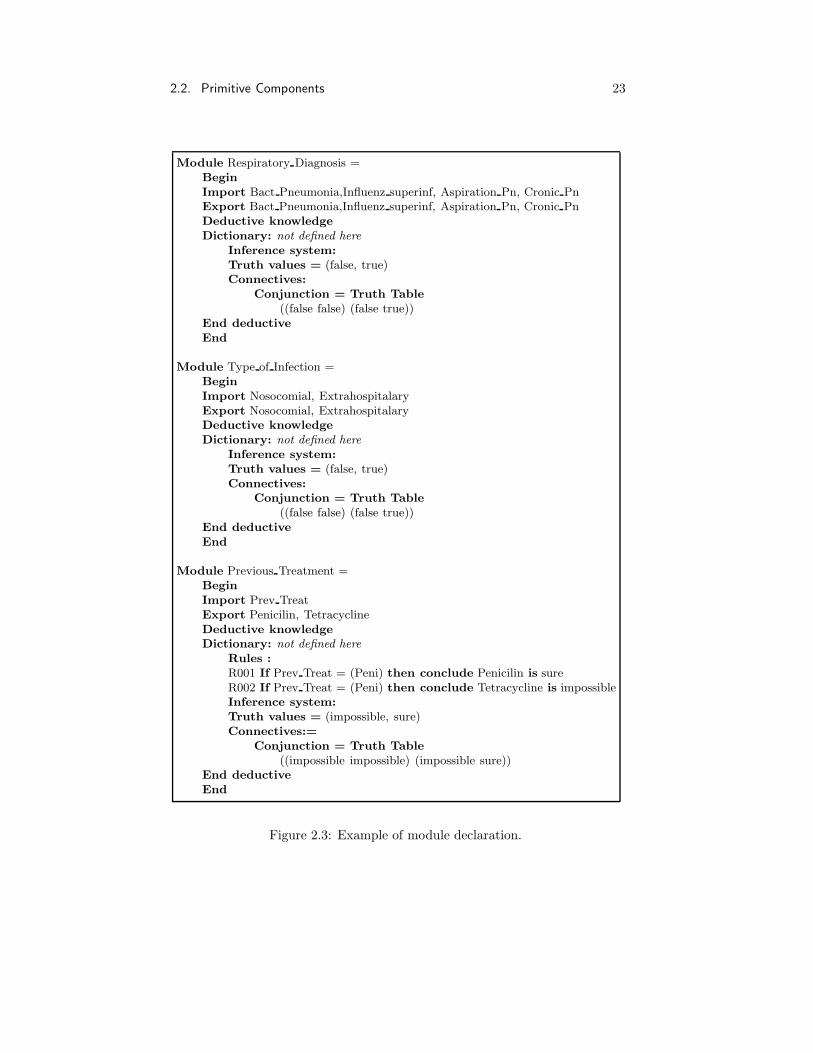
Imported facts are those facts whose values can be obtained from the userduring the execution of a module. For instance, the module Previous Treatmentof the Figure 2.3 has the following declaration:
Import Prev Treat
Imported facts like Prev Treat are asked when needed in the evaluation of amodule2. The code of a module containing an import declaration will be allowedto ask to the user for values of imported facts only. For instance the module ofthe previous example can only ask to the user for the value of the fact Prev Treat.
Exported facts are those facts that are visible outside the module. Theycan be asked by the user or by other modules. For instance, the module Previ-ous Treatment of the Figure 2.3 has the following export interface declaration:
Export Penicilin, Tetracycline
All the exported facts like Penicilin either have to be deduced by the kernelof the module or have to be imported by the module (obtained from the user).In this example the facts of the export interface can be deduced by the kernel bymeans of the rules R001 and R002. Notice that the facts of the export interfaceof the module Type of Infection of the Figure 2.3 are imported directly from theuser (Nocosomial and Extrahospitalary are facts that belong both to the exportand import interface of the module). Facts deduced and imported facts notmentioned in the export declaration of the module are hidden to the rest of themodules including the user, i.e., they cannot be used in the body of the restof the modules. A module with no exported facts is meaningless. However wecan access to the exported facts of its submodules as explained in subsectionaccess names below. The code of a module containing an export declaration willprovide means to answer questions about the values of the exported facts only.
2When and in which order the imported facts are asked to the user is determined by thetype of evaluation of the module. See the Section 5.3.
2.2. Primitive Components 23
Module Respiratory Diagnosis =Begin
Import Bact Pneumonia,Influenz superinf, Aspiration Pn, Cronic PnExport Bact Pneumonia,Influenz superinf, Aspiration Pn, Cronic PnDeductive knowledge
Dictionary: not defined here
Inference system:
Truth values = (false, true)Connectives:
Conjunction = Truth Table
((false false) (false true))End deductive
End
Module Type of Infection =Begin
Import Nosocomial, ExtrahospitalaryExport Nosocomial, ExtrahospitalaryDeductive knowledge
Dictionary: not defined here
Inference system:
Truth values = (false, true)Connectives:
Conjunction = Truth Table
((false false) (false true))End deductive
End
Module Previous Treatment =Begin
Import Prev TreatExport Penicilin, TetracyclineDeductive knowledge
Dictionary: not defined here
Rules :
R001 If Prev Treat = (Peni) then conclude Penicilin is sureR002 If Prev Treat = (Peni) then conclude Tetracycline is impossibleInference system:
Truth values = (impossible, sure)Connectives:=
Conjunction = Truth Table
((impossible impossible) (impossible sure))End deductive
End
Figure 2.3: Example of module declaration.
24 Chapter 2. Modularity
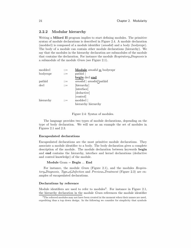
2.2.2 Modular hierarchy
Writing a Milord II program implies to start defining modules. The primitivesyntax of module declarations is described in Figure 2.4. A module declaration(moddecl) is composed of a module identifier (amodid) and a body (bodyexpr).The body of a module can contain other module declarations (hierarchy). Wesay that the modules in the hierarchy declaration are submodules of the modulethat contains the declaration. For instance the module Respiratory Diagnosis isa submodule of the module Gram (see Figure 2.1).
moddecl ::= Module amodid = bodyexprbodyexpr ::= pathid |
begin decl endpathid ::= amodid | amodid/pathid
decl ::= [hierarchy][interface][deductive][control]
hierarchy ::= moddecl |hierarchy hierarchy
Figure 2.4: Syntax of modules.
The language provides two types of module declarations, depending on thetype of body declaration. We will use as an example the set of modules inFigures 2.1 and 2.3.
Encapsulated declarations
Encapsulated declarations are the most primitive module declarations. Theyassociate a module identifier to a body. The body declaration gives a completedescription of the module. The module declaration between keywords beginand end contains the hierarchy, interface and kernel declarations (deductiveand control knowledge) of the module.
Module Gram = Begin ... End
For instance, the module Gram (Figure 2.1), and the modules Respira-tory Diagnosis, Type of Infection and Previous Treatment (Figure 2.3) are ex-amples of encapsulated declarations.
Declarations by reference
Module identifiers are used to refer to modules3. For instance in Figure 2.1,the hierarchy declaration in the module Gram references the module identifier
3The referred modules may not have been created in the moment when their names are used,expediting thus a top down design. In the following we consider for simplicity that symbols

2.2. Primitive Components 25
Respiratory Diagnosis with the following declaration:
Module D = Respiratory Diagnosis
In this case D is the internal name of the module Respiratory Diagnosis usedin the module that contains this declaration (Gram).
Access names
With the declarations contained in the above examples we obtain the mod-ule Gram which has four submodules: Respiratory Diagnosis, Type of Infection,Previous Treatment and Gram of Sputum. The internal names D, T, P and Scorrespond to these submodules. They are used to reference the facts exportedby each of this submodules.
Paths of module names (pathid) indicate how to access a module in the hier-archy of modules. A path to a module is composed by module names separatedby a slash character ”/”. For instance the path Gram/D references the modulePrevious Treatment.
The access to exported facts of modules is composed of a path to a module,the slash character and the name of the exported fact. For instance, to accessthe exported fact Extrahospitalary of module Type of Infection we can use thefollowing equivalent names4.
Type of Infection/Extrahospitalary≡ Gram/T/Extrahospitalary
Given a module we can access to the exported facts of that module and tothe exported facts of its submodules, using the adecuate paths.
We can use encapsulated declarations or declarations by reference dependingon the structure we want to give to our problem. If we use only encapsulateddeclarations we will produce a structure with only a top level module. All theother modules have to be accessed by means of paths of module names.
2.2.3 Semantics of modules
At this point it is interesting to give a formal description of the modular en-vironment of Milord II. After that we will extend this description with newelements. We will keep the same example of Figure 2.1.
A program is a table P from system module identifiers IdM to the set ofmodules M:
P = IdM → M
The set of system module identifiers IdM is a set of internal names to distin-guish the different modules (we will use names like mod1, . . . ,modi for the set
exist when they are referenciated, that is, there are already all the encapsulated declarationsthat are required.
4At the moment we consider that all the modules are visible. In the following Sections wewill see cases where not all the possible paths are allowed. For instance, the submodule T
could be hidden outside the module Gram.

26 Chapter 2. Modularity
M and > for the top module). The set of modules M = M ∪ > is composedby the set of modules M that are created from all the encapsulated moduledeclarations (begin ... end), plus a virtual module named > (top module).
In our example (Figures 2.1 and 2.3) there are five declarations of this type.They create a set of six module identifiers.
IdM = >,mod1,mod2,mod3,mod4,mod5
Each module m ∈ M is composed of the hierarchy (H), export (E), import(I) and kernel (K) components. The top module only contains the top levelhierarchy of modules (export5, import and kernel components are empty).
M = H × E × I × K
In the following to simplify the notation we will use Hm as the hierarchycomponent of a module m ∈ M6. Similarly for the export, import and kernelcomponents (Em, Im and Km respectively). The hierarchy of a module m ∈ Mis a function Hm from local submodule identifiers of the module m, Im, toidentifiers of the modules M (IdM ) and a visibility module qualifier (visible,hidden or open7).
Hm : Im → IdM × visible, hidden, open
Each module has its own function that points to its submodules. Followingthe same example, we will show the hierarchy components of those modules (seethe Figure 2.5). The top level module contains all the modules declared bymeans of encapsulated declarations at top level:
I> = Gram,Respiratory Diagnosis, Type of Infection,Previous Treatment,Gram of Sputum
H>(Gram) = (mod1, visible)H>(Respiratory Diagnosis) = (mod2, visible)H>(Type of Infection) = (mod3, visible)H>(Previous Treatment) = (mod4, visible)H>(Gram of Sputum) = (mod5, visible)
The module Gram has four submodules declared by reference:
Imod1= D,T, P, S
Hmod1(D) = (mod2, visible)
Hmod1(T ) = (mod3, visible)
Hmod1(P ) = (mod4, visible)
Hmod1(S) = (mod5, visible)
5As noticed above a module with empty export interface has no sense. In that case the topmodule is a special module and we are only interested in accessing the exported facts of itssubmodules.
6For instance the hierarchy of a module m could be expressed as Hm = first(P (m)), thefirst component of the tuple corresponding to identifier m.
7In Section 2.5.1 we will see open declarations of submodules. Now we consider all themodules are visible.
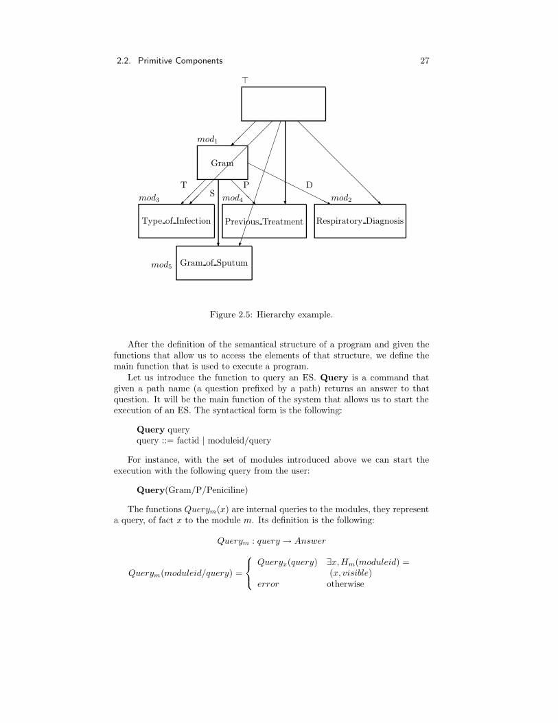
2.2. Primitive Components 27
@@
@R
?
HHHHHHHHHHj
@@
@@
@@
@@
@@R
?
Type of Infection
mod3
Gram of Sputummod5
Previous Treatment
mod4
Respiratory Diagnosis
mod2
Gram
mod1
>
DT PS
Figure 2.5: Hierarchy example.
After the definition of the semantical structure of a program and given thefunctions that allow us to access the elements of that structure, we define themain function that is used to execute a program.
Let us introduce the function to query an ES. Query is a command thatgiven a path name (a question prefixed by a path) returns an answer to thatquestion. It will be the main function of the system that allows us to start theexecution of an ES. The syntactical form is the following:
Query queryquery ::= factid | moduleid/query
For instance, with the set of modules introduced above we can start theexecution with the following query from the user:
Query(Gram/P/Peniciline)
The functions Querym(x) are internal queries to the modules, they representa query, of fact x to the module m. Its definition is the following:
Querym : query → Answer
Querym(moduleid/query) =
Queryx(query) ∃x,Hm(moduleid) =(x, visible)
error otherwise

28 Chapter 2. Modularity
Querym(factid) =
deducem(factid) if factid ∈ Em
error otherwise
Notice that when we query a module for a fact belonging to a submodule ofthat module, this module has to be visible. The execution of a query alwaysstarts on the top module. For instance, consider the command above, where theMilord II interpreter (INT ) makes a query to the top module of the currentES.
INT [[Query(Gram/P/Peniciline)]]Query>(Gram/P/Peniciline) =QueryH>(Gram)(P/Peniciline) =Querymod1
(P/Peniciline) =QueryHmod1
(P )(Peniciline) =Querymod4
(Peniciline) = deducemod4(Peniciline)
Finally the interpreter starts the deduction in the module mod4 (expressedby deducemod4
) in order to give a value to the fact Peniciline. We will returnto this point along the thesis. We have introduced the modular structure ofa program from the semantic point of view. In the following we will extentthis semantical description adding new components that we will progressivelyintroduce.
2.3 Generic modules
The instantiation of a generic module is considered as a module declaration. Thedefinition of generic modules opens to the user the possibility of defining specificoperations of composition of modules. Generic modules are then operations (orfunctions) on modules. This standard technique to define generic modules is theone to define functions, that is, it consists of isolating a piece of program, ormodule, from its context and then abstracts it by specifying:
1. Those modules upon which the abstracted module may depend (require-ments or parameters of the generic module).
2. The contribution of the abstracted module to the rest of the program(results or export interface of the generic module).
As we said the obvious example of this technique is functional programming,where such abstractions (functions) form the basic program units. The func-tional body defines how to compute the output (results) in terms of the input(requirements). The method for building large KB systems consists of applyinggeneric modules to previously built particular modules.
An example of definition of generic modules is presented in figure 2.6. Re-member the example used until now. The module Gram (Figure 2.1) has foursubmodules (Figures 2.3 and 2.8). The submodule S corresponds to the gramanalysis of sputum. Now the generic module Global Gram (Figure 2.6) repre-sents a general gram analysis over different samples. Global Gram can now be

2.3. Generic modules 29
applied to different modules to produce new modules analyzing different typesof samples. For instance, an equivalent of module Gram (named New Gram) canbe obtained by instantiating the generic module Global Gram with the moduleGram of Sputum.
Keeping the common parts in a generic module we can save code and timeand make the code much more understandable. Finally when a module isneeded to make the gram analysis of a sputum sample, it is only necessaryto put both modules together by a generic module application, for instanceGlobal Gram(Gram of Sputum).
In Figure 2.7 we extend the syntax of modules declaration of Figure 2.4adding the generic modules declarations.
The declaration of a generic module is like a normal module except that inthe hierarchy component of that module there are submodules with local namesthe parameters of the generic module. These submodule names point nothinguntil the instantiation of the generic module. Then the instantiation of a genericmodule consists in:
• Making a copy of the generic module.
• Solving the hierarchy component of that copy.
For instance, we can add to our current system the generic module Global Gram,as the new module mod6. The hierarchy component of that module is:
Hmod6(D) = (mod2, visible)
Hmod6(T ) = (mod3, visible)
Hmod6(P ) = (mod4, visible)
Hmod6(X) = ∅
To compute Global Gram (Gram of Sputum) we make then a copy of thatmodule (mod7) and solve the hierarchy component linking the submodule X withthe module Gram of Sputum. This is the module New Gram. It is equivalentto the previous one (Gram), except that the submodule X (Gram of Sputum) ishidden outside Global Gram.
Hmod7(D) = (mod2, visible)
Hmod7(T ) = (mod3, visible)
Hmod7(P ) = (mod4, visible)
Hmod7(X) = (mod5, hidden)
The parameters of a generic module are considered as submodules. If wewant to refer to exported facts of these submodules we must build a path withthe parameters names (for instance in the rules of the module Global Gram wehave X/CBGN).
The parameters of a generic module are submodules hidden outside thegeneric module. For instance, notice that the submodule X is hidden outsidethe new module New Gram. The following query is then wrong because thesubmodule X is hidden (Hmod7
(X) = (mod5, hidden)):

30 Chapter 2. Modularity
Module Global Gram (X) =Begin
Module D= Respiratory DiagnosisModule T= Type of InfectionModule P= Previous TreatmentExport Pneumococcus, Haemophilus, EnterobacteriaDeductive knowledge
Dictionary: not defined here
Rules:
R001 If X/DCGP then conclude Pneumococcus is possibleR002 If X/DCGP and D/Bact Pneumonia
then conclude Pneumococcus is very possibleR003 If X/BGN and D/Aspiration Pneumonia and T/Nosocomial
then conclude Enterobacteria is quite possibleR004 If X/CBGN and P/Penicilin then conclude Haemophilus is sureInference system:
Truth values= (impossible, few possible, sligh possible, possible,quite possible, very possible, sure)
Renaming =
D/False ==> impossibleD/True ==> sureT/False ==> impossibleT/True ==> sureP/impossible ==> impossibleP/sure ==> sureX/false ==> impossibleX/unlikely ==> [impossible, possible]X/may be ==> possibleX/likely ==> [possible, sure]X/true ==> sure
Connectives:
Conjunction: the same table defined in Figure 2.1.
end deductive
end
Module New Gram = Global Gram(gram of sputum)
Figure 2.6: Example of generic module definition and application.

2.3. Generic modules 31
moddecl ::= Module modbindmodbind ::= amodid [([paramlist])] [= bodyexpr]
bodyexpr ::= pathid[([iparamlist])] |
begin decl endparamlist ::= amodid | paramlist ; paramlistiparamlist ::= bodyexpr | iparamlist ; iparamlist
Figure 2.7: Syntax of generic modules.
Module Gram of Sputum =Begin
Import Sputum Clas, Sputum GramExport End, Gram yes, DCGP, CGPC, CGPR, BGN, CBGNDeductive knowledge
Dictionary: not defined here
Rules :
R001 If Sputum clas=(Grup 1,Grup 2,Grup 3)then conclude Sputum ok is true
R002 If Sputum clas=(Grup 4,Grup 5,Grup 6)then conclude Sputum not ok is true
R003 If Sputum ok then conclude Gram yes is trueR004 If Sputum not ok then conclude End is trueR005 If Sputum Gram=(DCGP MC) then conclude DCGP is trueR006 If Sputum Gram=(DCGP MC) then conclude CGPC is unlikelyR007 If Sputum Gram=(CGPC MC) then conclude CGPC is likelyR008 If Sputum Gram=(CGPC MC) then conclude DCGP is unlikelyR009 If Sputum Gram=(CGPR MC) then conclude CGPR is trueR010 If Sputum Gram=(BGN MC) then conclude BGN is likelyR011 If Sputum Gram=(CBGN MC) then conclude CBGN is likelyInference system:
Truth values = (false, unlikely, may be, likely, true)Connectives: ...
End deductive
End
Figure 2.8: Example of module used as parameter of a generic module.

32 Chapter 2. Modularity
INT [[Query(New Gram/X/CBGN)]]Query>(New Gram/X/CBGN) =QueryH>(New Gram)(X/CBGN) =Querymod7
(X/CBGN) = error
A generic module can use the exported facts of its module parameters, so theinstantiation of a parameter can not be made with any module, but only thoseexporting the needed facts. For instance the module Gram of Sputum exportsthe facts needed in the rules of the generic module Global Gram. In the followingwe will see how to make save the instantiations of generic modules by means ofdeclaring the parameters as refinements of another module (like giving a type tothe parameters).
We want to support the process of incremental KB building by means ofgeneric modules. So whenever the definition of a generic module changes, thesechanges must be reflected in the rest of the program. The way to do it is justto repeat the module applications that refer to the modified module. This re–linking process can be automatised by the compiler, so that the user gets rid ofthis task.
2.4 Refinement, Expansion and Contraction
Before explaining these operations on modules we need to know which are themain components of the kernel of modules. It is not our purpose here to ex-plain in detail the kernel of modules. We only give a short description of themain semantical components of the kernel which are needed to understand theexplanations of the current Chapter.
The kernel of modules is composed of the deductive and the control knowl-edge (see the Figure 2.9) . Deductive knowledge is composed of the definitionof facts (dictionary), the rules and the definition of the local logic (inferencesystem). At the moment we consider the kernel of a module composed of thefollowing set8: dictionary, rules, logic and control.
The kernel of a module m ∈ M is composed by the dictionary (Dm), therules (Rm), the logic (Lm) and the control (Cm).
K = D × R × L × C
So far we have described modules and generic modules. These declarationsare enough to write programs. Now we introduce the operations that allow usto deal with incremental programming in Milord II. These operations are therefinement, expansion and contraction of modules.
Top–down programming methodology is related to an incremental specifica-tion of problems. We have seen that modular decomposition of problems is auseful technique to simplify the programming task. We can think in a program
8The complete explanation of the deductive and control knowledge will be done in Chap-ters 4 and 5 respectively. Here we only explain what is needed to understand the concept ofinheritance which is closely related to modularity and affects mainly the kernel of modules.
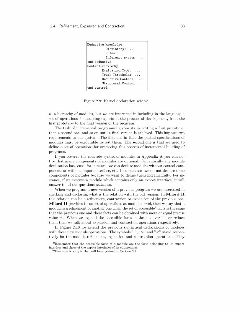
2.4. Refinement, Expansion and Contraction 33
Deductive knowledge
Dictionary: ...
Rules: ...
Inference system: ...
end deductive
Control knowledge
Evaluation Type: ...
Truth Threshold: ...
Deductive Control: ...
Structural Control: ...
end control
Figure 2.9: Kernel declaration scheme.
as a hierarchy of modules, but we are interested in including in the language aset of operations for assisting experts in the process of development, from thefirst prototype to the final version of the program.
The task of incremental programming consists in writing a first prototype,then a second one, and so on until a final version is achieved. This imposes tworequirements to our system. The first one in that the partial specifications ofmodules must be executable to test them. The second one is that we need todefine a set of operations for overseeing this process of incremental building ofprograms.
If you observe the concrete syntax of modules in Appendix A you can no-tice that many components of modules are optional. Semantically any moduledeclaration has sense, for instance, we can declare modules without control com-ponent, or without import interface, etc. In some cases we do not declare somecomponents of modules because we want to define them incrementally. For in-stance, if we execute a module which contains only an export interface, it willanswer to all the questions unknown.
When we program a new version of a previous program we are interested inchecking and declaring what is the relation with the old version. In Milord IIthis relation can be a refinement, contraction or expansion of the previous one.Milord II provides these set of operations at modular level, then we say that amodule is a refinement of another one when the set of accessible9 facts is the samethat the previous one and these facts can be obtained with more or equal precisevalues10. When we expand the accessible facts in the next version or reducethem then we talk about expansion and contraction operations respectively.
In Figure 2.10 we extend the previous syntactical declarations of moduleswith these new module operations. The symbols ”:”, ”>” and ”<” stand respec-tively for the module refinement, expansion and contraction operations. They
9Remember that the accessible facts of a module are the facts belonging to its exportinterface and those of the export interfaces of its submodules.
10Precision is a topic that will be explained in Section 3.2.

34 Chapter 2. Modularity
can be used in all the module declaration including the parameter declarationof generic modules.
moddecl ::= Module modbindmodbind ::= amodid [([paramlist])] [modoper modexpr]
[= modexpr]modexpr ::= bodyexpr | bodyexpr modoper modexprbodyexpr ::= pathid[([iparamlist])] |
begin decl endparamlist ::= amodid modoper modexpr |
paramlist ; paramlistiparamlist ::= modexpr | iparamlist ; iparamlistmodoper ::= : | > | <
Figure 2.10: Syntax of refinement, contraction and expansion.
All these modular operations are based in three functions: the enrichementverification, the inheritance and the information hiding. Now we explain therefinement of modules that is the operation that uses these three functions. Theother operations are modifications of this refinement operation.
2.4.1 Refinement
When we design a module the first decision is which is the set of goals of thatmodule. These goals are represented by the set of accessible facts of that module,those of its export interface and those of the export interfaces of its submodules.When we design by refinement a new version of that module we must maintainthe same set of goals. Furthermore we must guarantee that these goals will beobtained with better or equal precision in the new version.
Consider the example of Figure 2.11. The module Sample only contains anexport interface. The expression Module Gram of Sputum : Sample = be-gin ... end declares11 that the module Gram of Sputum is a refinement of themodule Sample. This is the idea of incremental programming, all the modulesthat are refinements of the module Sample (they represent samples) must keepthe same export interface. The module Gram of Sputum is a refinement of themodule Sample because it has the same export interface and other components(for instance, the deductive one) that allows the module to obtain better resultsfor the exported facts (different from unknown as was the case for the moduleSample because it has not deductive component).
This is specially useful when we declare generic modules. Remember thatthe instantiation of a generic module implies to assign submodules to the genericmodule. The resultant module should use the exported facts of the submodules
11There is an equivalent notation for it: Module Gram of Sputum = begin ... end :
Sample.

2.4. Refinement, Expansion and Contraction 35
Module Sample =Begin
Export End, Gram yes, DCGP, CGPC, CGPR, BGN, CBGNEnd
Module Gram of Sputum : Sample =Begin
Export End, Gram yes, DCGP, CGPC, CGPR, BGN, CBGNDeductive knowledge
Dictionary: not defined here
Rules :
R001 If Sputum clas=(Grup 1, Grup 2, Grup 3)then conclude Sputum ok is true
...End
Figure 2.11: Example of generic module definition and application.
assigned. It is obvious that not all the modules can be used to instantiate ageneric module. For instance, we can modify the previous declaration of thegeneric module Global Gram as following:
Module Global Gram (X : Sample) =Begin the same declarations than in Figure 2.6 End
This kind of declaration assure us that the modules used to instantiate thegeneric module Global Gram are refinements of the module Sample having thesame export interface (for instance, we can assure that these module will exportthe fact X/CBGN needed in the evaluation of the module).
We obtain a new module from two modules by means of a refinement oper-ation. We obtain the module Gram of Sputum refining the second declarationof Figure 2.11 by the module Sample. A refinement operation is composed bythree operations: the enrichement verification, the inheritance and the informa-tion hiding.
We will explain these components by considering the following equivalentdeclarations:
Module M = M 1 : M 2 ≡ Module M : M 2 = M 1
In the following consider that the internal identifier of the modules M 1 andM 2 are mod1 and mod2 respectively. The internal identifier of the new moduleM is mod. For instance if we consider that all the declarations are at top level,then: H>(M) = mod, H>(M 1) = mod1 and H>(M 2) = mod2.

36 Chapter 2. Modularity
Enrichement Verification
Given a refinement step it is necessary to verify the enrichement of information.We take the following definition of enrichement between two modules.
Definition 2.1 (Enrichement) We say that the module M 1 is an enriche-ment of the module M 2, if and only if:
1. Emod2⊆ Emod1
2. Imod2⊆ Imod1
and ∀x ∈ Imod1∩ Imod2
. Hmod1(x) is an enrichement of
Hmod2(x) or Hmod1
(x) = ∅
3. ∀x ∈ Emod1∩ Emod2
. V (x,mod1) is more precise than V (x,mod2).
4. Lmod1= Lmod2
or Lmod1= ∅.
That means that the module M 1 can extend the export interface and thesubmodules of M 2. When a submodule is declared in both modules M 1 andM 2, they must preserve the enrichement relation. Finally we must obtain moreprecise values for the facts that belong to both export interfaces (precision willbe the topic of Section 3.2, at the moment we can consider better values).
Inheritance
When we declare a module as a refinement of another one we can maintainseveral components of the last version, to avoid the expert write twice the com-mon components. Copy inheritance acts over submodules, facts defined in thedictionary and the local logic of the module.
When we declare the new version of a module by refinement we could declarenew submodules and we must declare the same submodules that in the previousversion (remember that Imod2
⊆ Imod1). In these declarations we could omit the
body of some of them. That means that the module M will inherit the bodiesof the submodules of M 2 that not are present in the declaration of M 1. Inthe case of declaring a body in M 1 for a module declared yet in M 2 then arefinement relation is performed between the two submodules.
For all the submodules x that are in Imod1∩ Imod2
, the submodules of theresultant module are:
Hmod(I) =
Hmod2(I) Hmod1
(I) = ∅
(first(Hmod1(I)) : first(Hmod2
(I)), second(Hmod2
(I))) otherwise
The refinement operation makes a copy of the non modified elements of thedictionaries.
Dmod = x|x ∈ Dmod1or x ∈ Dmod2
and x 6∈ Dmod1

2.4. Refinement, Expansion and Contraction 37
In the case of the logic, the module inherits the logic of module M2 if thatmodule contains a logic declaration.
Lmod =
Lmod2if Lmod1
= ∅Lmod1
if Lmod16= ∅
Information Hiding
The first component of the refinement operation was the enrichement verifica-tion. One of the conditions to obtain a refinement relation between two modulesis that the accessible facts of both modules must be the same. Then after check-ing the enrichement of information we must hide the new accessible facts of therefined module if any.
In a refinement operation information hiding affects the export interface andthe modular structure of the module created by the refinement. All the exportedfacts of M 1 not present in the export interface of M 2 are hidden in the resultingmodule M. Similarly all the submodules of M 1 not present in the hierarchy ofM 2 are hidden in the resulting module M.
Until now we have considered that all modules are visible except for theparameters of generic modules. Here we introduce the concept of hidden sub-modules. When a module contains a submodule that is hidden, this submodulecan not be referenced outside the module. The new module can reference thefacts in the export interface of all its submodules, but from outside the modulewe can not access the hidden submodules.
Finally the components of the module M , after checking the enrichement ofinformation, considering inheritance and information hiding will be the following:
• Emod = Emod2
• Imod = Imod1
• Imod = Imod1∪ Imod2
Hmod(I) =
Hmod2(I) If Hmod1
(I) = ∅and I ∈ Imod1
∩ Imod2
(first(Hmod1(I)) : first(Hmod2
(I)) I ∈ Imod1∩ Imod2
, second(Hmod2(I)))
(first(Hmod1(I)), hidden) I ∈ Imod1
− Imod2
• Dmod = x|x ∈ Dmod1or x ∈ Dmod2
and x 6∈ Dmod1
• Lmod =
Lmod2if Lmod1
= ∅Lmod1
if Lmod16= ∅
• Rmod = Rmod1
• Cmod = Cmod1

38 Chapter 2. Modularity
We have a small example of the refinement operation in Figure 2.12 and 2.13.Consider the first version of the program in Figure 2.12. It is composed ofthree modules that only contain submodule declarations and the interfaces.The module Global Culture S has two submodules named Gram S and Respi-ratory Diagnosis. The module Gram S has only the submodule Respiratory Di-agnosis.
Module Global Culture S =Begin
Module G = Gram SModule D = Respiratory diagnosisExport Pneumococcus isolation, Haemophilus isolation,
Staphylococcus isolation, No microorganism isolation, antibiogramImport Multiresistant microorganismEnd
Module Gram S =Begin
Module D= Respiratory DiagnosisImport Nosocomial, Extrahospitalary, Prev Treat, Sputum clas,
Sputum GramExport Pneumococcus, Haemophilus, Staphylococcus, EnterobacteriaEnd
Module Respiratory Diagnosis =Begin
Import Bact Pneumonia,Influenz superinf, Aspiration Pn, Cronic PnExport Bact Pneumonia,Influenz superinf, Aspiration Pn, Cronic PnEnd
Figure 2.12: Example of module refinement.
In the next version of the program in Figure 2.13 we can see how the moduleGlobal Culture is defined as a refinement of the previous module Global Culture S.It is easy to see that the module Global Culture is a refinement of the moduleGlobal Culture S because they have the same export interfaces and the samesubmodules. Then the enrichement verification test success and there is noinformation hiding. The only operation is the inheritance of components, inparticular the bodies of the submodules D and G.
The declaration of the module Gram is a little different because this modulecontains more submodule declarations than module Gram S.
IH>(Gram S) = D
IH>(Gram) = D,T, P, S
Then information hiding acts over the submodule structure and the new mod-ules Type of Infection, Previous Treatment and Gram of Sputum become hidden
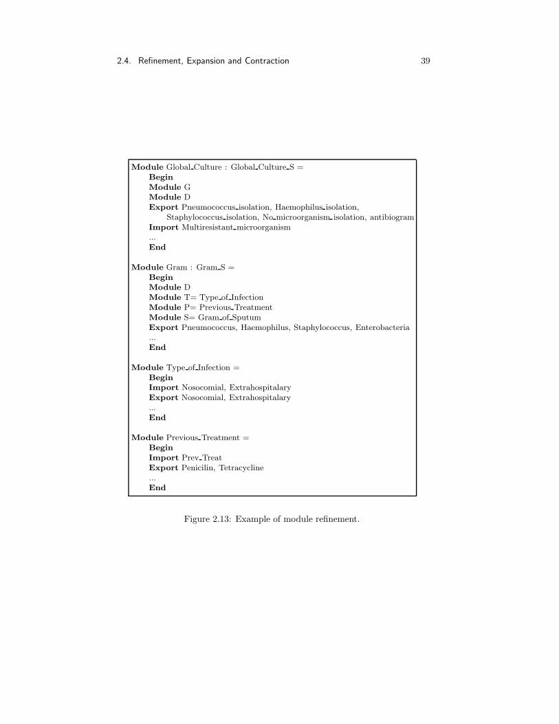
2.4. Refinement, Expansion and Contraction 39
Module Global Culture : Global Culture S =Begin
Module GModule DExport Pneumococcus isolation, Haemophilus isolation,
Staphylococcus isolation, No microorganism isolation, antibiogramImport Multiresistant microorganism...End
Module Gram : Gram S =Begin
Module DModule T= Type of InfectionModule P= Previous TreatmentModule S= Gram of SputumExport Pneumococcus, Haemophilus, Staphylococcus, Enterobacteria...End
Module Type of Infection =Begin
Import Nosocomial, ExtrahospitalaryExport Nosocomial, Extrahospitalary...End
Module Previous Treatment =Begin
Import Prev TreatExport Penicilin, Tetracycline...End
Figure 2.13: Example of module refinement.

40 Chapter 2. Modularity
from outside the module Gram. Notice that the import interface of that modulehas changed because the facts imported by the module Gram are now importedby its submodules.
Finally we can see in Figure 2.14 the modular structure of the program. Themodules Type of Infection, Gram of Sputum and Previous Treatment are hiddeninto module Gram. For instance, the paths
Global Culture/Gram/Type of Infection/NosocomialGlobal Culture/Gram/Previous Treatment/Penicilin
are incorrect, but the paths
Global Culture/Respiratory Diagnosis/Bact PneumoniaGlobal Culture/Gram/Respiratory Diagnosis/Bact Pneumonia
are correct and equivalent. Another equivalent modular structure could be todeclare the submodule D of module Global Culture S as:
Module D = Gram S/D
@@
@R
?
HHHHHHHHHHj
@@
@@
@@
@@
@@R
Type of Infection
Gram of Sputum
Previous Treatment Respiratory Diagnosis
Gram
Global Culture
Figure 2.14: Visibility example (hidden modules are written in italic).
2.4.2 Expansion and Contraction
Expansion and contraction operations are based on the refinement one. Expan-sion allows to build modules that are an expansion of a previous version. We

2.5. Special declarations 41
can extend the set of accessible facts or add submodules to the previous version.As in the refinement case to expand modules we test that the new module isan enrichement of the previous one. Inheritance of components is performed asin the refinement operation, but information hiding is not applied because weallows the expert to program an expansion of a previous module. Consider thefollowing declaration:
Module M = M 1 > M 2
The components of a module M created by means of the above declaration arethe following (we represent only the components that are different of a refinementoperation):
• Emod = Emod1
• Imod = Imod1∪ Imod2
Hmod(I) =
Hmod2(I) if Hmod1
(I) = ∅and I ∈ Imod1
∩ Imod2
(first(Hmod1(I)) > first(Hmod2
(I)) I ∈ Imod1∩ Imod2
, second(Hmod2(I)))
Hmod1(I) I ∈ Imod1
− Imod2
Contraction only test an inverse enrichement verification. Given the decla-ration Module M = M 1 < M 2 we only test that M 2:M 1 holds. Inheritanceand information hiding are not applied.
2.5 Special declarations
We complete in this Section the set of module declarations allowed in Milord II.Open and Inherit submodule declarations are only programming facilities andthey do not belong to the primitives of the modular language. Dynamic modulesis an important characteristic of Milord II that allows us to execute submoduledeclarations at run time.
One form of the composition of modules is achieved by mean of the decla-ration of submodules. This declarations defines the hierarchical component of amodule. The complete syntax of the hierarchy component of modules is givenin Figure 2.15.
2.5.1 Inherit and Open
When we use by reference submodule declarations we usually declare a local namefor the submodule. If we want to preserve the previous name of the submodulewe can use the following submodule declaration:

42 Chapter 2. Modularity
hierarchy ::= moddecl |Inherit pathid |Open bodyexpr |Sharing patheq |hierarchy hierarchy
Figure 2.15: Syntax of submodule declarations.
Inherit B ≡ Module B = B
Obviously this type of declaration can only be used in by reference declarationsof modules.
The last type of submodule declaration is a special kind of submodule dec-laration, the notion of a submodule as open.
Open B
In this case it is not necessary to use paths to access the facts exported by thesubmodule B. All the facts exported by the submodule belongs to the module.It is valid with encapsulated or by reference declarations.
It is easy to see that name clashes can occur when we use declarations oftype open. If a module has more than one opened submodule, the names of theexported facts must be different12.
The submodules of the open module are visible directly without the path tothe open module. Consider the following abstract example in Figure 2.16. Wecan access to the facts C/c, C/a and C/B/b. The paths C/A/a and C/A/B/bare not valid.
Module A =Begin
Module B = Begin Export b ... End
Export a... End
Module C =Begin
Open AExport c... End
Figure 2.16: Example of open module.
12Milord II Compiler (Arcos, 1992) detects all these conflicts.

2.5. Special declarations 43
2.5.2 Sharing
Considering that Milord II allow us to define applications incrementally, insome cases we are interested in giving to the compiler information about whichmodules will be finally the same module. These declarations assure that in thebuilding process the compiler will detect the violations of this previous declara-tions. Syntax declaration of sharing is given in Figure 2.17.
sharing ::= Sharing patheqpatheq ::= pathid = patheq | pathid = pathid |
patheq ; patheq
Figure 2.17: Syntax of sharing.
For instance in the current example we can declare:
Sharing Respiratory Diagnosis = Gram/D
This declaration means that the module Respiratory Diagnosis has to be thesame module that the submodule D of the module Gram.
Sharing declaration can be used at top level or in the hierarchy declarationsof modules. In the last case local names are used. The last declaration impliesthat:
H>(Respiratory Diagnosis) = H>(Gram/D)
Sharing declaration can also be used in generic module declarations. In thedeclarations above sharing was only to give the information that some moduleswill be the same. In the case of generic modules sharing declarations affectthe future instantiations of those generic modules. For instance, consider thefollowing declaration:
Module G(X : X S; Y : Y S; Sharing X/A = Y/B) =Begin ... End
This declaration means that when we instantiate the generic module G withtwo modules, the first module X must contain a submodule named A and thesecond one Y a submodule named B, and these two submodules must be thesame.
2.5.3 Dynamic Modules
Milord II deals with dynamic modules by means of dynamic links among mod-ules at run time. This characteristic allows us to implement powerful particularcontrol strategies.
Despite the creation of dynamic modules belongs to the control knowledgeof modules (see Section 5.4.4) we introduce briefly those declarations.
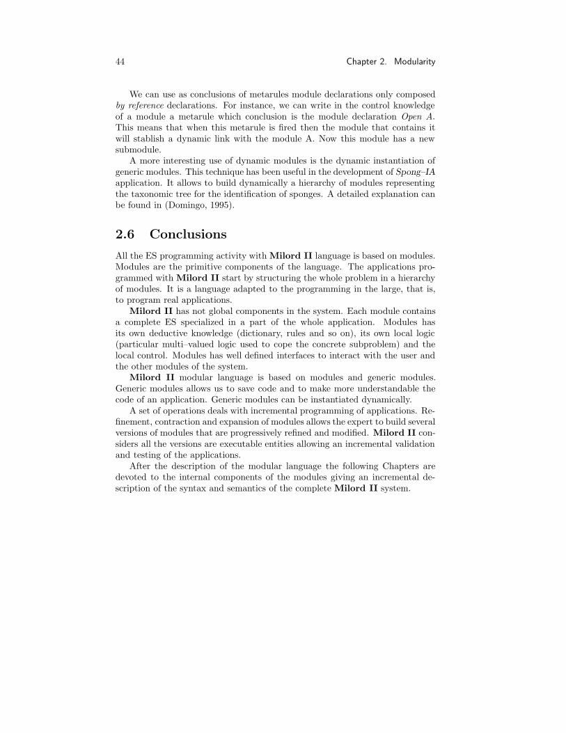
44 Chapter 2. Modularity
We can use as conclusions of metarules module declarations only composedby reference declarations. For instance, we can write in the control knowledgeof a module a metarule which conclusion is the module declaration Open A.This means that when this metarule is fired then the module that contains itwill stablish a dynamic link with the module A. Now this module has a newsubmodule.
A more interesting use of dynamic modules is the dynamic instantiation ofgeneric modules. This technique has been useful in the development of Spong–IA
application. It allows to build dynamically a hierarchy of modules representingthe taxonomic tree for the identification of sponges. A detailed explanation canbe found in (Domingo, 1995).
2.6 Conclusions
All the ES programming activity with Milord II language is based on modules.Modules are the primitive components of the language. The applications pro-grammed with Milord II start by structuring the whole problem in a hierarchyof modules. It is a language adapted to the programming in the large, that is,to program real applications.
Milord II has not global components in the system. Each module containsa complete ES specialized in a part of the whole application. Modules hasits own deductive knowledge (dictionary, rules and so on), its own local logic(particular multi–valued logic used to cope the concrete subproblem) and thelocal control. Modules has well defined interfaces to interact with the user andthe other modules of the system.
Milord II modular language is based on modules and generic modules.Generic modules allows us to save code and to make more understandable thecode of an application. Generic modules can be instantiated dynamically.
A set of operations deals with incremental programming of applications. Re-finement, contraction and expansion of modules allows the expert to build severalversions of modules that are progressively refined and modified. Milord II con-siders all the versions are executable entities allowing an incremental validationand testing of the applications.
After the description of the modular language the following Chapters aredevoted to the internal components of the modules giving an incremental de-scription of the syntax and semantics of the complete Milord II system.

Chapter 3
Approximate Reasoning
We have seen in Chapter 2 that the natural form of describing and solvingproblems was by means of the decomposition of the problems into subproblems.As shown Milord II deals with structured problem solving integrating andadapting known modularization techniques into a reach ES shell.
A module of Milord II contains the necessary components to describe thedomain and control knowledge relative to a problem, by means of facts, rules,metarules, and so on. Till now we have not described these internal componentsof a module. We only have considered that a module is able to produce itemsof information (export interface) from others items of information that has beenprovided by the user (import interface) or by the submodules of that module(hierarchy).
This Chapter is devoted to explain the nature of those items of informationthat we name facts in ES’s terminology. For that we can consider that an item ofinformation is composed of four components, that is, object, attribute, value andconfidence (Dubois and Prade, 1988). The attribute is a function that attachesa value or a set of values to an object. The confidence indicates the reliabilityof an item of information.
Now we analyze the concepts of imprecision and uncertainty of an item ofinformation. The imprecision is a concept attached to the value component ofan item of information, and the uncertainty to the confidence one. For instance,we can say It is very possible that the temperature of the patient is between 36
and 38. In this example the object is the patient and the attribute is thetemperature. The value of the temperature is imprecise and it belongs to theinterval [36, 38] with a confidence degree of very possible. This is an exampleof an imprecise and uncertain proposition. We can think in other examples,a precise and certain proposition: The temperature of the patient is 36.7; animprecise and certain proposition: The temperature of the patient is between 36
and 38; and finally a precise and uncertain proposition: It is very possible thatthe temperature of the patient is 36.7.
The management of uncertainty and imprecision becomes essential to mod-elize real problems. Usually the kind of knowledge domains treated by ES’s
45

46 Chapter 3. Approximate Reasoning
contains imperfect knowledge. We can find many sources of imprecision anduncertainty. For instance, measurement devices have imprecise results (the cor-poral temperature depends on which part of the body we take the measure);subjective appreciations are imprecise (the valuation of the temperature touch-ing the patient with the hand); the incomplete knowledge added to the naturallanguage ambiguity produce uncertain propositions (If the patient has headacheit is possible that his temperature could be greater than 37 ).
In this Chapter we will explain how Milord II manages uncertainty andimprecision. As we will see it is limited to manage uncertain data or imprecisedata. It is not possible to express at the same time the uncertainty and theimprecision of an item of information.
When we want to manage uncertainty by means of linguistic terms (for in-stance, likely, possible, false, and so on) we must decide how many terms to useand which they are. Usually these questions are problem dependent and theyare related to the concrete meaning that the expert associates to these linguisticterms. Some problems could need five terms to express its uncertainty and an-other problem could need seven terms. Furthermore it is possible that the termpossible would have a different meaning for different experts, or that one expertprefers to use another term such as likely. The concrete set of terms used toexpress uncertainty and its granularity will depend on the expert criteria andon the concrete problem he is considering.
As seen in Chapter 2 each module is used to specify a subproblem. It couldbe very useful to change the language of representation of uncertainty in functionof the type of subproblem. The modular structure of Milord II together withits approach to uncertainty management, allows to define in a natural way localuncertainty calculus attached to each module, in such a way that the knowledgeadequation process can also be applied to the uncertainty management. Theinterest in having different uncertainty calculus in an ES becomes clearer whenexpert systems involving several human experts have to be built. Milord II sys-tem allows us to define local uncertainty logics in the modules and mechanismsof communication among these logics(Agustı et al., 1992).
This Chapter is divided in four parts. The first one is devoted to the definitionof algebras of truth–values. The expert must define which is the logic moreadecuated to his problem. This implies to define a set of linguistic terms usefulto express his knowledge (for instance, he would say The confidence degree thatthe patient has pneumonia is very possible or The treatment with ciprofloxacineis good). Furthermore the expert can express some control to the meaning ofthe logic operators. An example of this is to find the confidence degree of thefact fever from two sentences: It is slightly possible that the patient has headache; If the patient has headache it is possible that he has fever.
The second part contains an explanation in depth of the treatment givenby Milord II of the concepts of uncertainty and imprecision. This is reachedby extending the algebra of truth–values to an algebra of intervals of truth–values (we can say that The evidence that the patient has pneumonia is betweenpossible and very possible) and introducing fuzzy sets (for instance, The degree

3.1. Algebra of truth–values 47
of membership of the patient to the set of the tall people is quite).The third part is devoted to the communication between the local logics of
modules. When two modules use different logics (linguistic terms and opera-tors) we must find a mechanism of translation of the linguistic terms to makecompatible the communication between those modules (for instance, what is themeaning of the sentence Fever is possible for another module that do not usethis term, maybe Fever is likely?). Finally we introduce all the constructs of thelanguage Milord II that allow the experts to define the local logics of modules.
3.1 Algebra of truth–values
Psychological experiments (Kuipers et al., 1988; Fox, 1989) show that humanproblem solvers do not use numbers to deal with uncertainty and that the waythey manage it is situation dependent. These requirements were partially sat-isfied in the Milord system in the sense that the treatment of uncertainty wasbased in different operators defined over a set of linguistic terms describing theglobal verbal scale the experts use to express degrees of uncertainty (Godo etal., 1989).
The approach used in Milord II to manage uncertainty is based on many–valued logics. The use of many–valued logics has been criticized (Pearl, 1990;Hajek et al., 1992) because of the confusion between uncertainty and imprecision.We do not enter in depth in this kind of problems that has been extensivelytreated in the literature. Despite this, many–valued logics have been proved tobe useful in ESs (Turner, 1984; Bonissone et al., 1987; Godo et al., 1989; Lopezde Mantaras, 1990). We justify the use of many–valued logics because they havean efficient and simple deduction from the computability point of view. Wewill extend these logics with intervals of truth–values (Esteva et al., 1994) asa technique to manage uncertainty or imprecision. As we will see intervals oftruth–values allow us to deal with uncertain or imprecise information and tointroduce negative evidence in the sentences.
Here we present the definition of a family of many–valued logics which de-ductive system is based on a new kind of inference rule called specialization (itwill be presented in the next Chapter). Some aspects of these logics have beenalready described in (Agustı et al., 1991; Agustı et al., 1992). Each logic is de-termined by a particular algebra of truth–values from a parametric family thatis described next.
Definition 3.1 (Algebra of Truth–values) An algebra of truth–values is afinite algebra
AnT =< An,Nn, T, IT >
such that:
1. The ordered set of truth–values An is a chain of n elements:
0 = a1 < a2 < · · · < an = 1
where 0 and 1 are the boolean False and True respectively.

48 Chapter 3. Approximate Reasoning
2. The negation operator Nn is the unary operation defined as
Nn(ai) = an−i+1
the only one that fulfills the following properties:
N1: If a < b then Nn(a) > Nn(b), ∀a, b ∈ An
N2: N2n = Id.
3. The conjunction operation T is a binary operation such that the followingproperties hold ∀a, b, c ∈ An:
T1: T (a, b) = T (b, a)
T2: T (a, T (b, c)) = T (T (a, b), c)
T3: T (0, a) = 0
T4: T (1, a) = a
T5: If a ≤ b then T (a, c) ≤ T (b, c) for all c
4. The implication operator IT is defined by residuation with respect to T , i.e.
IT (a, b) = Max c ∈ An|T (a, c) ≤ b
and satisfies the following properties:
I1: IT (a, b) = 1 if, and only if, a ≤ b.
I2: IT (1, a) = a
I3: IT (a, IT (b, c)) = IT (b, IT (a, c))
I4: If a ≤ b, then IT (a, c) ≥ IT (b, c) and IT (c, a) ≤ IT (c, b) for all c
I5: IT (T (a, b), c) = IT (a, IT (b, c))
As it is easy to notice from the above definition, any of such truth–valuesalgebras is completely determined as soon as the set of truth–values An and theconjunction operator T are determined. So, varying these two characteristicswe can obtain a parametric family of different many–valued logics, including,among others, Kleene’s and Lukasiewicz’s logics.
As we can see in the example of the Figure 3.1 (the complete definition forthe module Gram of Sputum given in the Figure 2.8 and used in the previousexamples), this module declares a local logic (inference system) consisting in aset of linguistic terms (truth values) and the conjunction operator (conjunction).
The definition of this local logic in the module Gram of Sputum is deter-mined by the declaration of the set of five linguistic term S5 = false, unlikely,may be, likely, true, and the conjunction operation TS5
operation defined in theTable 3.1. The expert has chosen this number of terms because he considers thatit is sufficient to talk about the concepts contained in this module. The names

3.1. Algebra of truth–values 49
Module Gram of Sputum =Begin
Import Sputum clas, Sputum GramExport End, Gram yes, DCGP, CGPC, CGPR, BGN, CBGNDeductive knowledge
Dictionary: not defined here
Rules :
R001 If Sputum clas=(Grup 1 or Grup 2 or Grup 3)then conclude Sputum ok is true
R002 If Sputum clas=(Grup 4 or Grup 5 or Grup 6)then conclude Sputum not ok is true
R003 If Sputum ok then conclude Gram yes is trueR004 If Sputum not ok then conclude End is trueR005 If Sputum Gram=(DCGP MC) then conclude DCGP is trueR006 If Sputum Gram=(DCGP MC) then conclude CGPC is unlikelyR007 If Sputum Gram=(CGPC MC) then conclude CGPC is likelyR008 If Sputum Gram=(CGPC MC) then conclude DCGP is unlikelyR009 If Sputum Gram=(CGPR MC) then conclude CGPR is trueR010 If Sputum Gram=(BGN MC) then conclude BGN is likelyR011 If Sputum Gram=(CBGN MC) then conclude CBGN is likelyInference system:
Truth values = (false, unlikely, may be, likely, true)Connectives :
Conjunction = Truth Table
((false, false, false, false,false)(false, unlikely, unlikely,unlikely, unlikely)(false, unlikely, may be, may be, may be)(false, unlikely, may be, may be, likely)(false, unlikely, may be, likely, true)))
End deductive
End
Figure 3.1: Example of Local logic declaration.
false unlikely may be likely true
false false false false false false
unlikely false unlikely unlikely unlikely unlikely
may be false unlikely may be may be may be
likely false unlikely may be likely likely
true false unlikely may be likely true
Table 3.1: TS5Table.

50 Chapter 3. Approximate Reasoning
of the linguistic terms used in each module are intended to make understandablethe kind of the concepts that are used into the modules.
The expert can choose a T function (holding the properties T1–T5) de-pending on the meaning he wants to give to the conjunction operation1. Forinstance, considering that T (a, b) ≤ min(a, b) (from properties T4 and T5) theexpert can consider more or less optimistic evidence combinations. For instance,he can consider that the conjunction of two propositions with confidence degreelikely results on a confidence degree of may be (less than likely).
Nn
false true
unlikely likely
may be may be
likely unlikely
true false
Table 3.2: N5 Table.
It is easy to see that the negation operator N5 and the implication operatorITS5
can be deduced from the above definition of the algebra of truth–values (seethe Tables 3.2 and 3.3 respectively).
x / y false unlikely may be likely true
false true true true true true
unlikely false true true true true
may be false unlikely true true true
likely false unlikely likely true true
true false unlikely may be likely true
Table 3.3: ITS5(x, y) Table.
3.1.1 Modus Ponens Operator
The language used in Milord II is composed of weighted facts and rules. Tillnow we have only introduced the conjunction and negation operators. Then weshould also introduce the many–valued version of modus ponens inference rule(Alsina et al., 1984; Valverde and Trillas, 1985; Trillas and Valverde, 1987) thatallows us to make deductions, that is, to deduce the truth–value of the conclusionof a rule from the truth–values of its conditions and the truth–value of the rule.
1A general algorithm for finding truth–value algebras over a partially ordered set of n
elements is given in (Godo and Meseguer, 1991).

3.2. Uncertainty and Imprecision 51
Definition 3.2 (Modus Ponens) MPT is a function from An ×An to the setof intervals2 of An defined as:
MPT (a, b) =
∅ if a and bare inconsistent (*)
[a, 1] if b = 1T (a, b) otherwise
(*) a and b are inconsistent if there exists no c such that I T (a, c) = b.
This is a functional expression of the multiple–valued version of the classicalmodus ponens rule, i.e. MPT (a, b) is the set of solutions for ρ(q) in the equationsystem:
ρ(p) = aρ(p → q) = IT (ρ(p), ρ(q)) = b
where ρ is the valuation of the sentences.The modus ponens table for S5 and TS5
is given in Figure 3.4. For instance,if the value of the fact p is likely and the value of the rule p → q is true, by meansof the definition of the MPT function and the Table TS5
we can deduce that thefact q has the value likely. We will return over this rule when we explain thespecialization of KB’s in Chapter 4.
x / y false unlikely may be likely true
false ∅ ∅ ∅ ∅ [false,true]
unlikely false ∅ ∅ ∅ [unlikely,true]
may be false unlikely ∅ ∅ [may be,true]
likely false unlikely ∅ may be [likely,true]
true false unlikely may be likely [true, true]
Table 3.4: MPTS5(x, y) Table.
We know how to use a propositional language (no defined yet) with negation,conjunction and implication operators. Till now we only have talked about thededuction by means of the modus ponens inference rule. In Chapter 4 we willintroduce a different kind of deduction based on the specialization inference rule(SIR).
3.2 Uncertainty and Imprecision
We have considered in the introduction that uncertainty and imprecision takean important role in the data used by ESs. Now we will talk on the concrete
2Notice that the modus ponens operator can return an interval of truth–values. This willbe one of the reasons to introduce intervals of truth–values as we will see.

52 Chapter 3. Approximate Reasoning
items of information that can be used in Milord II. Our system deals withuncertainty and imprecision by means of the use of intervals of linguistics terms.
Consider the following two examples:
1. Peter is quite tall.
2. It is possible that Peter is tall.
These two propositions can be confusing. When we read the first propositionwe could think that the fact of being tall is a graduated measure, then we aretalking about the value of the attribute tall. There are persons that are clearlytall (for instance, those that their height is greater than 2m.) and persons thatare clearly not tall, but between these two categories there are persons that areslightly tall, quite tall, etc.
Another interpretation can guide us to the concept of fuzzy sets. The differ-ence between a classic set (named crisp set) and a fuzzy set is that the elementsof the considered universe have a degree of membership to the fuzzy set. In crispsets the elements of the universe belong or not belong to the crisp set. We canconsider that the concept tall is a fuzzy set. We can imagine then a characteristicfunction that given the height of a person it returns the degree of membershipof the person to the fuzzy set tall (see the Figure 3.2), expressed by means oflinguistic terms (like quite).
µF (ω)
1.9
-
6
1
1.7 2.50ω
Figure 3.2: Fuzzy set representing the concept tall.
The second proposition can be interpreted as the first one, but its syntacticalform guides us to think that tall is a boolean concept (a person is tall or nottall) and we have a degree of confidence on the fact that Peter is tall. In thiscase we are talking about uncertainty. We are not sure if Peter belongs or notto the set tall.
There are other examples where that confusion is not possible, for instance,we can say that It is possible that Peter has pneumonia but we can not talk

3.2. Uncertainty and Imprecision 53
about degrees of pneumonia (it is not possible to say that somebody is quitepneumonic). These interpretations depend on the concept and the concretelinguistic terms we are using.
In Milord II we will consider only information of the second type, that is,uncertain information expressed by means of linguistic terms, but the seman-tical interpretation of those sentences will be dependent on the set of conceptsthe expert is using. We will take advantage of this confusion3 to introduceimprecision.
Imprecision at truth level
Milord II introduces imprecision at the truth level by means of intervals oflinguistic terms. One may know that a proposition must take a truth–value butdoes not know exactly which, then a set of possible values is given. We can saythat The confidence degree of pneumonia is between possible and very possible.
This kind of imprecision could seem not to be very useful. We can think thatusers would have difficulty to interpret these intervals of truth–values, but wewill make it clear by comparing the interpretation of these intervals in Milord IIwith the interpretation of truth–values in Milord.
In Milord all the truth–values associated to the facts were considered to bepositive evidences. When we found more than one deductive path to evaluate afact, we choose the best, that is, that of the greatest truth–value. In Milord thegoal was to obtain the maximum certainty degree for the facts. Furthermore inthe case that the fact would get a truth–value less than a threshold, it would beconsidered unknown (there was no sufficient positive evidence to consider it).
Now we can comment the interpretation of positive evidence by means ofintervals of truth–values. We consider that positive evidence is an interval froma truth–value to true, that is, when we say that the value of the fact pneumonia ispossible, the interpretation is that the value of pneumonia belongs to the interval[possible, true]. When a fact belongs to the interval [0, 1] it means that we knownothing about its value. With this interpretation when we obtain the value falsefor a fact it means that the value of this fact is unknown instead of false.
Thanks to this interpretation we can introduce negative evidence as intervalsof truth–values of the form [0, ai], that is, the value of the fact could be fromfalse to ai. In Milord II we interpret positive and negative evidence as before.We can find deductive paths with positive and negative evidences. The resultof the parallel combination is the fusion (intersection) of these intervals (as wewill see in Section 4.2.3). Then the interpretation of an interval as [a i, aj] is thatthe positive evidence is ai, but there are a negative evidence aj. The goal ofMilord II is to obtain the maximum precision of the value of facts. We willreturn on this in the following Sections.
3Experience shows that experts use this kind of interpretation. Depending on the set ofconcepts they are using the interpretation of the linguistic terms could be taken as values orconfidence degrees.

54 Chapter 3. Approximate Reasoning
Imprecision at value level
If we return to the examples above we can interpret the imprecision at truth levelas imprecision at value level, the more standard one. When we say that It isbetween possible and very possible that Peter is tall we could think of a previousimprecise measure of the height of Peter (a numeric interval). The characteristicfunction of the fuzzy set tall is a function from intervals of height to intervals ofdegrees of membership to the fuzzy set tall.
In the following Section we will present the extension of the algebra of truth–values to the algebra of intervals. Now we consider that the sense of theseintervals is the imprecision at truth level. We will return on imprecision at valuelevel in Section 4.4.1.
3.2.1 Intervals of Truth–values
We have presented several semantic motivations to introduce intervals of truth–values, but there are other reasons. The first one is related to the chaining ofrules. We can see in the above definition of the modus ponens inference rulethat in some cases it returns an interval of truth–values. The second reasonis to make possible the mappings between different local logics and it will beexplained in Section 3.3.
The deductive system of Milord II works on the set of intervals of An,Int(An). N∗
n, T ∗ and MP ∗T are the point–wise extensions4 of Nn, T and MPT
respectively. Let us introduce more formally the intervals of truth–values andthese operators.
Definition 3.3 (Intervals) Int(An) will stand for the set of intervals of An,i.e.
Int(An) = [a, b]|a, b ∈ An such that a ≤ b ∪ ∅
being [a, b] = c ∈ An|a ≤ c ≤ b.
Notice that there exists an embedding from An to Int(An) identifying ele-ments a with intervals [a, a] of Int(An). For the sake of simplicity on the nota-tion, we will also denote by a the interval [a, a] when no confusion is possible.The interval ∅ represents an inconsistent value as we will see.
On the set of intervals Int(An) we can define the imprecision ordering andthe uncertainty ordering (Esteva et al., 1994).
Imprecision ordering: Is naturally induced by the set inclusion relationship⊆. Given A,B ∈ Int(An) , the interval A is more precise or equal thanB, if and only if A ⊆ B (see Figure 3.3 for an example on Int(A4), whereA4 = 0, a, b, 1). The goal of Milord II is to produce the most precisevalues.
Uncertainty ordering: The uncertainty order of An can be extended intoInt(An) in at least two different ways:
4Strictly speaking they give the minimal interval containing the point–wise extensions.

3.2. Uncertainty and Imprecision 55
PPPPPPPPPPPPi
ZZ
ZZ
>
1Z
ZZZ
ZZ
ZZ
>
>
ZZ
ZZ
>
ZZ
ZZ
>
ZZ
ZZ
>
ZZ
ZZ
>
∅
1ba0
[b,1][a,b][0,a]
[a,1][0,b]
[0,1]
Figure 3.3: Imprecision Ordering on Int(A4).
• Weak uncertainty order (see Figure 3.4):
[a1, b1]≤[a2, b2] if, and only if, a1 ≤ a2 and b1 ≤ b2
• Strong uncertainty order:
[a1, b1] [a2, b2] if, and only if, b1 ≤ a2 or [a1, b1] = [a2, b2]
Now we will define the negation, conjunction and modus ponens operatorsfor the intervals of truth–values.
Definition 3.4 We define on the set of intervals of An the functions N ∗n and
T ∗ as those functions that give the minimal interval containing the point–wiseextensions of Nn and T respectively. That is:
• N∗n([a, b]) = [Nn(b),Nn(a)]
• T ∗([a, b], [c, d]) = [T (a, c), T (b, d)]
In order to get a functional expression of the multiple–valued version of theModus Ponens rule, we also define on the set of intervals of An the functionMP ∗
T as follows:
Definition 3.5 For any truth–intervals V and W , we define MP ∗T (V,W ) as
the minimal interval containing all solutions for z in the family of functionalequations
IT (a, z) = b
varying a ∈ V and b ∈ W .

56 Chapter 3. Approximate Reasoning
ZZ
ZZ~
ZZ
ZZ~
>
>ZZ
ZZ~
>
ZZ
ZZ~
>ZZ
ZZ~
>
ZZ
ZZ~
>
1ba0
[b,1][a,b][0,a]
[a,1][0,b]
[0,1]
Figure 3.4: Weak Uncertainty Ordering on Int(A4).
This definition can be made more explicit when taking into account that thetruth–intervals W attached to rules of Milord II are always upper intervals, i.e.W is of the form W = [c, 1].
Proposition 3.1 MP ∗T ([a, b], [c, 1]) = [T (a, c), 1]
After the introduction of the intervals and its operators we will explain brieflyhow we work with intervals and the concept of precision.
3.2.2 Working with intervals
We have seen the extension to an algebra of intervals of truth–values. Now wecan explain how these intervals are used in practice with the rules of Milord II.
The goal of Milord system was to find the maximum truth–value for the factsbecause it only uses rules with positive evidence. Because of the use of intervalsof truth–values, the goal of Milord II is to obtain the maximum precisioninterval for the facts (combining positive and negative evidences).
Consider a set of rules with the same fact in the conclusion, but some ruleswith the negation of that fact in their conclusion. Then we should consider thefollowing points:
• The rules with a positive conclusion (not negated) will fix the minimumcertainty value of the conclusion fact.
• The rules with a negative conclusion will fix the maximum certainty valueof the conclusion fact.
• We combine evidences by means of the intersection of intervals.

3.2. Uncertainty and Imprecision 57
We can explain it through an example. Consider that the weighted sentencesare pairs (sentence, value). And consider the following sentences (two facts andtwo rules)5:
(a, ρa)(b, ρb)(a → c, [ρr1
, 1])(b → ¬c, [ρr2
, 1])
From these facts and rules we can obtain a value for the sentence c and for¬c using the modus ponens inference rules for intervals of truth–values. Noticethat the value of a Milord II rule is an upper–interval to 1. The values for thesentences in the conclusions of those rules are then upper–intervals.
(a, ρa)(b, ρb)(a → c, [ρr1
, 1])(b → ¬c, [ρr2
, 1])(c,MP ∗
T ([ρa, ρa], [ρr1, 1])) = (c, [T (ρa, ρr1
), 1])(¬c,MP ∗
T ([ρb, ρa], [ρr2, 1])) = (¬c, [T (ρb, ρr2
), 1])
Using the negation operator of intervals of truth–values we obtain an intervalfrom 0 for the conclusion of the second rule. As commented before the positiverule produces a positive evidence of the conclusion and the negative rule a neg-ative one. The fusion (intersection) of intervals results in a interval where itsminimum value corresponds to a positive evidence and the maximum value tothe negative one.
(c, [T (ρa, ρr1), 1])
(¬c, [T (ρb, ρr2), 1]) ⇒ (c, [0,Nn(T (ρb, ρr2
))])
⇒
(c, [T (ρa, ρr1),Nn(T (ρb, ρr2
))])
When the intersection of values is empty, then it is considered to be incon-sistent. All the operators N ∗
n, T ∗ and MP ∗T with an argument equal to ∅ return
the same inconsistent value ∅.
3.2.3 Fuzzy Sets
Facts are one of the most primitive component of Milord II that represent theconcepts we will use in an ES. To deal with uncertainty and imprecision weassociate an interval of truth–values to the facts. Sometimes it is interesting todeal with other type of facts that represents set concepts. For instance, we canconsider that the fact treatment is a set of antibiotics. We could be interestedin comparing different treatments by means of set relations and operations.
From the logical point of view the concept of fuzzy set is carried out bychanging the usual definition of the characteristic function of a set by means of
5Notice that Milord did not use negation in the conclusion of rules.

58 Chapter 3. Approximate Reasoning
degrees of membership. We use uncertainty in the knowledge we possess aboutthe membership relation. To define a fuzzy set F we give a reference set Ω anda mapping, µF (ω), of Ω into [0, 1]. µF (ω), for ω ∈ Ω is interpreted as the degreeof membership of ω in the fuzzy set F . When µF (ω) ∈ 0, 1,∀ω, F is the sameas an ordinary subset of Ω. This is called a crisp subset of Ω and is a particularcase of fuzzy sets.
That is the usual definition of fuzzy sets as a mapping of the characteris-tic function into the interval [0, 1]. Because of the use of linguistic terms andimprecision we will extent the usual definition to the intervals of truth–values.
Now we put an example of fuzzy set named treatment. Consider the followingreference set, in this case a set of antibiotics:
Ω = carbamacepina, teofilina, digoxina ,dicumarinics, ciclosporina,difenilhidantoina
We use as imprecise degree of membership intervals of linguistic labels Int(An)of the logic of the module that contains this fact. We can specify a fuzzy set bymeans of its characteristic function. For instance, we consider that a treatmentis a fuzzy set composed by antibiotics6. The characteristic function of the facttreatment could be:
µtreatment(carbamacepina) = [impossible, impossible]µtreatment(teofilina) = [definite, definite]µtreatment(digoxina) = [impossible, definite]µtreatment(dicumarinics) = [very possible, very possible]µtreatment(ciclosporina) = [possible, very possible]µtreatment(difenilhidantoina) = [impossible, impossible]
After the definition of this kind of facts representing fuzzy sets we should sayhow to use them in the rules. We can use them by comparing different fuzzy sets.For instance, consider two different treatments in the universe of antibiotics. Wecan say If treatment1 is a subset of the treatment2 then ... or If the treatment1intersects with the treatment2 then .... This kind of operations and relationsresults in an interval of truth–values as we will see.
Elementary Operations and Relations
Here we explain the possible operations and relations among fuzzy sets used inMilord II. They are based on usual concepts used in fuzzy set theory and oper-ations among fuzzy sets (Zadeh, 1965). This provides to the experts a completetool to work with fuzzy sets. First of all we describe the unary operations usingthe above example.
Cut: We can use a threshold α to obtain a set Fα called α–cut of F . Thedefinition is the following:
Fα = ω ∈ Ω|min(µF (ω)) ≥ α
6This kind of facts like treatment are named enumerated facts in Milord II.

3.2. Uncertainty and Imprecision 59
Fα contains all the elements of Ω that are compatible with F at level atleast α. In Milord II α is the threshold of the module (see the Section 5.2)that contains the fact F . The threshold in the modules express the mini-mum certainty value that is considered to be significant. Suppose α to bepossible in the above example, then it is easy to see that:
treatmentpossible = teofilina, dicumarinics, ciclosporina
Core: The cut of F at level 1 is called the core of F , denoted F .
F = ω ∈ Ω|µF (ω) = 1
It contains all the elements of Ω that are in F at level 1. Following thesame example we can see that:
˙treatment = teofilina
Support: The support set contains all the elements of Ω that are not at level0.
S(F ) = ω ∈ Ω|min(µF (ω)) > 0
In our example they are all the elements with certainty value greater thanimpossible.
S(treatment) = teofilina, dicumarinics, ciclosporina
Complement: Complementation of set F is defined as the set F that has thefollowing characteristic function:
∀ω, µF (ω) = N∗n(µF (ω))
In the same example the characteristic function associated to the set¯treatment is:
µ ¯treatment(carbamacepina) = [definite, definite]µ ¯treatment(teofilina) = [impossible, impossible]µ ¯treatment(digoxina) = [impossible, definite]µ ¯treatment(dicumarinics) = [slightly possible, slightly possible]µ ¯treatment(ciclosporina) = [slightly possible, possible]µ ¯treatment(difenilhidantoina) = [definite, definite]
We consider the normal union and intersection operations among fuzzy sets:
Union: ∀ω, µF∪G(ω) = max∗(µF (ω), µG(ω))
Intersection: ∀ω, µF∩G(ω) = min∗(µF (ω), µG(ω))

60 Chapter 3. Approximate Reasoning
These operations are compatible with those on crisp sets7. Finally we explainthe set of relations we can use in Milord II. These relations given two fuzzysets return an interval of truth–values.
R : P(U) × P(U) → Int(An)
Before that we define the combination of relations and the complement of arelation as:
Combination: (R ∗ S)(F,G) = min∗(R(F,G), S(F,G))
Complement: R(F,G) = N ∗n(R(F,G))
Now we define the inclusion, intersection and equality between two fuzzy setsand its meaning.
Inclusion or equal:R⊆(F,G) = min∗(µF∪G)R⊇(F,G) = R⊆(G,F )
Intersection degree:R∩(F,G) = max∗(µF∩G)
Equality: R=(F,G) = (R⊆ ∗ R⊇)(F,G)
Inclusion:R⊂(F,G) = (R⊆ ∗ R=)(F,G)R⊃(F,G) = R⊂(G,F )
These relations return degrees of inclusion, intersection and equality betweentwo fuzzy sets. Using them we can express the degree of intersection of twotreatments, as so on.
All these operations are the most standard (Zadeh, 1965) and they are com-patible with crisp sets. In these definitions we have used for simplicity thefunctions min and max, but we can use instead the more general ones, thetriangular norm T and the triangular conorm S(x, y) = N(T (N(x),N(y))).
3.3 Local Logics
The need of communication among modules with different local uncertainty cal-culus has lead us to analyze the correspondence between uncertainty calculus.Uncertainty calculus can be considered as inference mechanisms defining logi-cal entailment relationships. Therefore the correspondences (or communication)between different calculus can be analyzed as mappings between different entail-ment systems. To do that we will introduce a summary of the main theoreticalresults on mappings between entailment systems (Agustı et al., 1992) and wepropose an algorithm to find the mappings that allow modules to communicate.
7We consider the functions maximum and minimum as the point–wise extensions:max∗([a, b], [c, d]) = [max(a, c),max(b, d)] and min∗([a, b], [c, d]) = [min(a, c), min(b, d)]

3.3. Local Logics 61
3.3.1 Mappings between different local logics
Let M and M ′ be two modules and (L,`) and (L′,`′) their corresponding logics,L and L′ standing for the languages and `′ and ` for the entailment relationsdefined on L and L′ respectively. To establish a correspondence from moduleM to module M ′, a mapping H : L → L′ relating their languages, is needed.In the following we will analyze some natural requirements for the mapping Hwith respect to the entailment systems ` and `′. Henceforth Γ and e will denotea set of formulas and a formula of L respectively.
A) If Γ ` e, then H(Γ) `′ H(e)
With this requirement we assure that for every formula deducible from a setof formulas Γ in M , its corresponding formula in M ′ by the mapping, H(e),will also be deducible in M ′ from the corresponding formulas of H(Γ). In otherwords, there is no inferential power lost when translating from M to M ′ througha mapping H satisfying A. Nevertheless the main drawback of requirement Ais that it does not forbid to deduce from H(Γ), in M ′, formulas that are nottranslations of any formula deducible from Γ in M . The property means that, inthe case of modules representing different experts, an expert E ′ related to M ′,using knowledge coming from an expert E related to M , will be able to deducethe same facts than E, but not only those facts. We need:
B) If H(Γ) `′ H(e), then Γ ` e
This is the inverse requirement of A. So, in this case all deductions in M ′
involving only translated formulas from M are translations of deductions in M ,or equivalently if a fact is not deducible in M , then its correspondent fact in M ′
will neither be deducible from the translated knowledge. An alternative to Bcould be:
C) If H(Γ) `′ e′, then there exists e such that Γ ` e and H(e) `′ e′.
This requirement assures that every formula deducible from H(Γ) in M ′ mustbe in agreement with what can be deduced from Γ in M . This requirement isslightly different from B, in the sense that it not necessary that e′ be exactly atranslation of a deducible formula e from Γ, but only something deducible fromsuch a translation. In the framework of logics for uncertainty management, e′ canbe interpreted as a weaker form of e, i.e. a formula expressing more uncertaintythan e.
It is worth noticing that, if C denotes the consequence operator with respectto an entailment system (L,`), that is, C(Γ) = e ∈ L|Γ ` e for all set offormulas Γ, then the requirements A and B can be rewritten in the followingway:
A) H(C(Γ)) ⊂ C ′(H(Γ))
B) C′(H(Γ)) ⊂ H(C(Γ))
being C ′ the consequence operator associated to the entailment system (L′,`′).

62 Chapter 3. Approximate Reasoning
From these three different requirements we can define the conditions on themappings in order these requirements hold. Notice that they are mappings oftruth–values algebras8.
Theorem 3.1 Given two truth–values algebras AnT1
=< An,Nn, T1, IT1> and
BmT2
=< Bm,Nm, T2, IT2>, a mapping H : An → I(Bm) fulfills the requirements
A or B or C from AnT1
to BmT2
if the following conditions hold:
1. H is non–decreasing, i.e. if a ≤ b, then H(a) ≤∗ H(b)
2. H(0) = 0
3. H(Nn(x)) = N∗m(H(x))
4. We have one case for each requirement:
A) H(T1(x, y)) ⊃ T ∗2 (H(x),H(y))
B) H(T1(x, y)) ⊂ T ∗2 (H(x),H(y))
H(x) ⊂ H(y) ⇒ x = y
C) H(T1(x, y)) ⊂ T ∗2 (H(x),H(y))
Finally we explain the algorithm that allows us to find mappings that arequasi–morfisms.
We can divide every chain An in three subsets:
• Nn = x|x < Nn(x)
• Fn = x|x = Nn(x)
• Pn = x|x > Nn(x)
We consider three subsets N ∗n , F∗
n and P∗n for the case of intervals Int(An).
In that case we use the weak uncertainty order defined before.
• N ∗n = x|x<Nn(x)
• F∗n = x|x = Nn(x)
• P∗n = x|x>Nn(x)
After that we find all the mappings
Hi : Nn ∪ Fn → N ∗m ∪ F∗
m
such that:
1. Hi(0) = 0
8The mappings are from the elements of a chain to elements of the set of intervals of theother chain.

3.3. Local Logics 63
2. Hi(Fn) ∈ F∗m
3. If x ≤ y then Hi(x) ≤∗ Hi(y), where x ∈ An and y ∈ Int(Bm).
Now we can extend these mappings:
H(x) =
Hi(x) if x ∈ Nn ∪ Fn
N∗m(Hi(H(x))) if x ∈ Pn
Finally we must check which mapping is quasi–morfisms for the three criteria,that is, checking the condition 4 of the quasi–morfism definition.
3.3.2 Example
For this example we will consider the set of modules used as examples in Chap-ter 2. Consider the module Gram (Figure 2.1) that has four submodules Res-piratory Diagnosis, Type of Infection, Previous Treatment (see Figure 2.3) andGram of Sputum (Figure 2.8).
Consider the following sets of truth–values corresponding to these modules,Gram7 for the module Gram and D2, T2, P2 and S5 for its submodules:
Gram7 = impossible, few possible, sligh possible, possible,quite possible, very possible, sureD2 = false, trueT2 = false, trueP2 = impossible, sureS5 = false, unlikely, may be, likely, true
and the T functions TS5and TGram7
(see Tables 3.1 and 3.5 respectively). Wedo not represent the other T functions because they are boolean logics withdifferent names for true and false. This is the situation of Figure 3.5 where weneed to find the mappings HT , HS, HP and HD.
impos few p sli p possib quite p very p sure
impos impos impos impos impos impos impos impos
few p impos few p few p few p few p few p few p
sli p impos few p sli p sli p sli p sli p sli p
possib impos few p sli p possib possib possib possib
quite p impos few p sli p possib very p very p very p
very p impos few p sli p possib quite p very p very p
sure impos few p sli p possib quite p very p sure
Table 3.5: TGram7Table.
First we focuses over the more difficult mapping HS. Following the abovedefinitions we can see that the sets N5, F5, N ∗
7 and F∗7 are:

64 Chapter 3. Approximate Reasoning
@@
@R
?
HHHHHHHHHHj
Type of Infection
Gram of Sputum
Previous Treatment Respiratory Diagnosis
Gram
Gram7, TGram7
D2, TD2T7, TT2
P2, TP2
S5, TS5
HDHT HPHS
Figure 3.5: Mapping example.
N5 = false, unlikelyF5 = may beN ∗
7 = impos, few p, sli p, possib, [impos, few p],[impos, sli p], [impos, possib], [few p, sli p], [few p, possib],[sli p, possib]F∗
7 = possib, [few p, very p], [sli p, quite p], [impos, sure]
Here there are two mappings that are examples of those that hold the lastrequirement C:
S/false → impossibleS/unlikely → [impossible, few possible]S/may be → [few possible, very possible]S/likely → [very possible, sure]S/true → sure
S/false → impossibleS/unlikely → [impossible, slightly possible]S/may be → possibleS/likely → [quite possible, sure]S/true → sure
The other cases are very simple because the other logics are boolean. Thenwe can map the first term of those logics to the first term of the logic of themodule Gram. We can express the mapping as:
D/false → impossibleD/true → sure

3.4. Logic Declaration 65
P/impossible → impossibleP/sure → sure
Given a value from a submodule of the module Gram we can translate thatvalue by means of the mappings above.
3.4 Logic Declaration
After the presentation of the local logics used in Milord II, here we describethe syntactical declaration of the inference system of a module. Each modulecontains the inference system declaration9. It contains the declaration of theconcrete logic that will be used in a module and the mechanism of communicationwith the local logics of its submodules.
The inference system declaration contains the set of ordered truth–values An,the renaming mappings among the local logic and those of the submodules anda set of logic operators: negation, conjunction, disjunction and modus ponens(see Figure 3.6).
Inference system:
Truth values = (...)
Renaming: ...
Connectives:
Negation = ...
Conjunction = ...
Disjunction = ...
Inference patterns: ...
Modus ponens = ...
Figure 3.6: Logic declaration.
Now we will explain in depth these declarations specially to make clear themultiple possibilities of the language. Normally the logics used in Milord II areof the type explained till now, that is, the expert declare a set of truth–valuesand a T function. To experiment with another kind of logics we allow to declarecomplete logics.
3.4.1 Truth values
Truth values of a module can be defined given an ordered set of symbols repre-senting linguistic terms, where each symbol is a truth–value. For instance thedeclaration of the set A5 is:
9As explained in Chapter 2 a module can declare its inference system by means of theinheritance mechanism.
66 Chapter 3. Approximate Reasoning
Truth values = (impossible, sli possible, possible, very possible,sure)
Notice that given a truth value declaration, the first symbol is considered tohave the semantics of true and the last symbol of false.
To maintain the logic declaration style that was used in Milord there areanother possible form of declaring the truth–values. It consists in associating toeach linguistic term four real numbers in the interval [0, 1]. Then we can use atruth–values declaration of the following form:
Truth values = (impossible = (a,b,c,d) , ... )
They correspond to the representation of a fuzzy interval (see the Figure 3.7) by means of a trapezoidal approximation of a fuzzy interval, as was used inMilord.
µx
cb d
-
61
a
AAAAAAAAA
10
Figure 3.7: Trapezoidal approximation of a fuzzy interval.
3.4.2 Connectives
After the declaration of the set of truth–values of the local logic we must definethe connectives and inference pattern of the logic, that is, the negation, con-junction, disjunction and modus ponens operators. To do that we have threeoptions:
1. The standard one in Milord II is to define a set of truth–values and aconjunction connective by means of a table. Then the system generatesthe other connectives, that is, negation, disjunction and modus ponens asseen above.
2. We can declare the set of truth–values and all the connectives and modusponens by means of tables. In this case these connectives will be used by

3.4. Logic Declaration 67
the inference engine. This option is for experimentation with other logics.Obviously the map of local logics does not work with logics different fromthe standard of Milord II.
3. The last option is that of Milord. We can define the set of truth–valuesas fuzzy intervals and declare the conjunction by means of a function. Inthis case the other connectives and modus ponens are calculated by thesystem.
Notice that in all the cases we use the extension to intervals, including thelogics used in Milord.
Functions Declaration
Users can define logical functions, or they can use the predefined functions ofthe system.
The user can define these functions by different means:
• Defining a Truth Table for the first and second case. In Figure 3.8 there isan example of conjunction table declaration.
• By means of a S–expression or using a predefined function in the last case.
Conjunction = Truth Table
(( false false false false false )( false unlikely unlikely unlikely unlikely )( false unlikely may be may be may be )( false unlikely may be may be likely )( false unlikely may be likely true ))
Figure 3.8: Truth table declaration for TA5.
The predefined functions which can be used are the well known:
• Lukasiewicz: T (x, y) = max(0, x + y − 1)
• Zadeh: T (x, y) = min(x, y)
• Probabilistic: T (x, y) = xy
3.4.3 Renaming
Because a module has its own logic, it should have a procedure to translatethe certainty values used in its submodules. Then we introduce the constructrenaming to make this translation.

68 Chapter 3. Approximate Reasoning
Renaming:
S/false ==> impossibleS/unlikely ==> [impossible,few possible]S/may be ==> [few possible,very possible]S/likely ==> [very possible,sure]S/true ==> sure
Figure 3.9: Renaming declaration example.
In Figure 3.9 there is an example of renaming declaration for the moduleGram with the logic B7 that has a submodule named Gram of Sputum that hasthe local logic A5.
Finally we can include the complete declaration from the logic point of viewof the module Gram (see the Figure 3.10).
3.5 Conclusions
In this Chapter we have introduced the local logics of modules of Milord II.Expertise implies to deal with imperfect information. The information managedby experts is imprecise and uncertain. A language for ESs must provide thepossibility of expressing easily this kind of information. Furthermore the moreadecuated language to express uncertainty is problem dependent.
Milord II introduces a family of multi–valued algebras that are useful torepresent uncertainty by means of linguistic terms. The extension of these al-gebras to intervals of truth–values has been used to deal with imprecision andfuzzy sets.
Finally local logics has been introduced as a form to adapt the logic to theconcrete problem and the method to allow the communication among moduleswith different logics has been provided.

3.5. Conclusions 69
Module Gram =Begin
Module D= Respiratory DiagnosisModule T= Type of InfectionModule P= Previous TreatmentModule S= Gram of SputumExport Pneumococcus, Haemophilus, Staphylococcus, EnterobacteriaDeductive knowledge
...Truth values= (impos, few p, sli p, possib, quite p, very p, sure)Renaming
D/false ==> imposD/true ==> sureT/false ==> imposT/true ==> sureP/impossible ==> imposP/sure ==> sureS/false ==> imposS/unlikely ==> [impos, sli pos]S/may be ==> possibleS/likely ==> [quite p, sure]S/true ==> sure
Connectives:
Conjunction = Truth Table
((impos, impos, impos, impos, impos, impos, impos)(impos, few p, few p, few p, few p, few p, few p)(impos, few p, sli p, sli p, sli p, sli p, sli p)(impos, few p, sli p, possib, possib, possib, possib)(impos, few p, sli p, possib, very p, very p, very p)(impos, few p, sli p, possib, quite p, very p, very p)(impos, few p, sli p, possib, quite p, very p, sure))
end deductive
... end
Figure 3.10: Example of logic declaration.

70 Chapter 3. Approximate Reasoning

Chapter 4
Deduction by Specialization
We have seen in Chapter 2 how an application can be structured in modules. Af-ter that we have introduced in Chapter 3 the concept of local logics in modules.This allowed us to deal with different uncertainty and imprecision languages indifferent modules. Following the top–down description of Milord II, in thisChapter we will analyze the deductive knowledge of modules and its interpreta-tion.
The deductive knowledge of Milord II is mainly composed of facts andrules as usual in Rule Based Systems . The particular kind of interpretationwe give here to deductive knowledge, that is, our inference engine, is a keyaspect of Milord II. We think that conventional inference engines produce apoor behavior of the ESs. We think of conventional inference engines as the wellknown backward and forward ones. In order to improve the behavior of ESs wepropose an inference engine based on a new rule of inference called specialization.The deduction in Milord II is based on the specialization of KBs as we will see.
This Chapter is divided in three parts. The first one is devoted to the kind ofbehavior we want ESs to have, as the main motivation to introduce our conceptof specialization of KBs. To do that we introduce informally the inference engineof Milord II. In the second part we present the logical foundation of the special-ization calculus and the theoretical results about it. After that we will explainin detail the actual inference engine which is based on specialization. Finallywe present all the extralogic components of deductive knowledge of Milord IIintroduced in the language to make easier the development of applications.
4.1 Enriched Behavior
The deductive knowledge component of the Milord II language is used byexperts to represent the domain knowledge of their applications. Like Milord,Milord II is based on facts of order 0+ and production rules with uncertainty.They have proved to be useful in our application development experiences. Forthis reason further discussions on knowledge representation are avoided except
71

72 Chapter 4. Deduction by Specialization
to motivate the introduction of new constructs.In this Chapter we are interested in showing that the interpretation of the
deductive knowledge plays an important role in the whole behavior of an ES,and that a good inference engine design can improve this behavior with respectto the one imposed by conventional inference engines.
At the moment, to simplify the explanation, we will focus the attention onthe interpretation of facts and rules without the extra complications of controldeclarations and modular structuration1.
E.S.
query
input
answer
explanation
success solution
failureunknown
dialog
goalquestions
SolutionsValidation
Figure 4.1: Standard Behavior of an ES.
In the Figure 4.1 there is represented the standard behavior of an ES. We willuse that Figure to make clear which are the general aspects we are interested in.These are related to the communication of the ES with the user, the solutionsgenerated by the ES and the validation of the ES.
Communication: First the user queries the system for the deduction of a fact.This fact will be the current goal of the ES2and the ES will try to findsolutions for that fact. In order to obtain solutions, the ES stablishes adialog with the user. The system asks questions to the user3, raised by theprocess of deduction. We consider that the communication is the sequenceof questions made to the user until a solution for the goal or a failure isfound.
Solutions: The system makes inferences using the rules and the answers givenby the user. Finally the system answers to the user with the solutions forthe goal (if found), which is normally a truth–value in ESs with uncertainty.Furthermore the system gives some explanation of its answer. We considerthat a solution is a pair composed by an answer and the explanation tothat answer.
Validation: The aspects above allow experts to think in some kind of validationof their system. The simplest one is case validation, that is, to compare a
1Despite we abstract from modular structure, some aspects of the communication betweenan ES and the user can be extended to the communication between modules. In the text youwill find references to modular structure when needed.
2We consider that the goals of the ES are facts. This corresponds to the interpretation ofmodules as objects able to answer facts that belongs to its export interface.
3In Milord II the facts asked to the user correspond to the imported facts of modules.

4.1. Enriched Behavior 73
case (the answers given by the user to the ES questions, the goal and itssolution by the user) with the corresponding solution obtained by the ES.
Communication, Solutions and Validation depend on the inference engineused. Conventional inference engines based on forward and backward strategiespresent a number of shortcomings in all three mentioned aspects of ES behavior.Milord was based on a backward inference engine with uncertainty. The archi-tecture and behavior of the inference engine of Milord II have been designedto improve these three aspects of ES behavior.
Following these aspects we will analyze the insufficient behavior produced byconventional inference engines and explain what are the improvements on it wepropose by means of an inference engine based on specialization. The first pointconsidered is the architecture of Milord II inference engine. The second andthird points are about one of the main topics of this thesis, that is, specialization.
4.1.1 Communication
In Chapter 1 we have explained that most of the applications developed withMilord II are interactive. Part of the problem solving behavior of the systemconsists in asking to the user the relevant information relative to the case tobe solved. The user’s confidence on the system is then highly related to thequestion–answer dialog he maintains with the ES. The user expects a sequenceof questions which should be clearly related to the current goal. The questionsasked and the order in which they are asked are very important to have a goodinteraction.
Conventional inference engines have search and deduction interleaved in thesame process. For instance, in backward inference engines depth first and breathfirst strategies are part of the design of the inference engine. The search strategyof Milord was depth first. That means that an inference engine has a fixed searchstrategy. The search strategy is embedded in the inference engine and it can notbe changed. Because the search strategy determines indirectly the questionsasked and the order in which they are asked, it is difficult with these inferenceengines to obtain a good user interaction. The way to change it is usually bychanging the order of rules, the order of the premises of the rules, and so on.
In this thesis we have not developed a theory of user system interaction. Herethe very important point we consider is the architecture of Milord II inferenceengine which makes easier to have a good user interaction (see Figure 4.2). Itis composed of two independent processes, that is, the search process and thedeductive process.
Search process: Given a goal, the search process computes the informationneeded to reach the goal with maximum precision (comments on maxi-mum precision and maximum certainty can be found in Section 3.2). InMilord II this process is independent of the deductive one. Classical in-ference engines are limited to the strategies implicitly implemented in theinference engine (depth first, breadth first, etc). This characteristic allows

74 Chapter 4. Deduction by Specialization
us to implement different search strategies independently of the deductiveprocess, including the conventional ones.
Deductive process: The inference engine of Milord II is based on special-ization of KBs. Each new fact known will specialize the KB. The knownfacts have been previously selected by the search process. Then the cur-rent status of a KB is specialized with respect to the known information.Specialization will be explained along this Chapter.
The proposed architecture allows us to implement different search strategiesdepending on different criteria and independently of the deductive process. Thesearch process is a part of the control of Milord II, and it will be explainedin depth in Chapter 5. The deductive process is the main topic of the currentChapter.
KB
DeductiveProcess
Specialization
Search Process
ControlStrategy
USERanswer
questions inpu
t
data fo
r
spec
ializa
tion
Figure 4.2: Inference Engine Architecture.
4.1.2 Solutions
A solution given to the user should be as much informative as possible, thatis, the answer and its explanation should be clearly related to the previousquestion–answer interaction with the user. Any doubt on this relation causesthe confidence in the system be on the decrease.
Real world ESs applications are very big and they demand a lot of interactionwith the user. Sometimes the user does not know the answer to ES questions.There are different reasons for that. Maybe the user actually does not knowthe answer to the system question, or he does not know it at the time of theinteraction. Frequently it can be too expensive to obtain that answer. Forinstance in medical environments, sometimes to answer a question implies to

4.1. Enriched Behavior 75
produce an intrusive action on the patient. For all these reasons it is veryimportant to be able to deal with incomplete information (lack of answers).Conventional inference engines are not able to work with incomplete information,they answer unknown to a goal if the system is not able to deduce the goal usingthe information given by the user.
Remember the standard ES behavior (please return on Figure 4.1). The userqueries to the system whether a given fact can be deduced. If the system is ableto deduce the fact, its certainty value is given back. Otherwise the answer isunknown (open world assumption). This behavior is rather poor because thesystem usually has much more information obtained implicitly in the process ofdeduction that could be useful to the user, for instance:
1. When the system is able to answer the user’s query, the user might alsobe interested in knowing other deductive paths that would be useful toimprove the solution, or to know other conditioned conclusions that couldbe deducible from this solution.
2. When the system is not able to answer a query, it gives back the valueunknown maybe because the user did not provide enough information tothe system. Thus, the communication would be much more informativeif the system was able to answer, not unknown, but give the informationthe user should know to come up with a value for the query (this kind ofanswers are called conditioned answers).
All this information the ES has about the goal is usually not visible outsidethe system, and it could be used to better modelise communication among hu-man experts. Looking carefully at how experts communicate their knowledgeand at their problem solving procedures, we can find complex communicationpatterns. Sometimes experts cannot reduce their interaction only to the com-munication of certainty values for facts, that is, by giving a precise answer. Forinstance, in medical diagnosis, when experts communicate, they also need:
1. To condition their decisions. Suppose that it is not known whethera patient is allergic to penicillin. An expert considering the possibility ofgiving penicillin as treatment would say: Penicillin is a good treatmentfrom a clinical point of view provided that the patient has no allergy topenicillin.
2. To give suggestions that must be considered with solutions. Ex-perts usually give other suggestions (antibiogram) that are related to thesolution (pneumococcus). For instance the expert might say: Pneumococ-cus has been isolated in the culture of sputum. In this case it is stronglysuggested to make an antibiogram to the patient .
3. To give conditioned suggestions to be considered together withdecisions. Another example of complex communication is the combina-tion of the above two communication patterns: Ciprofloxacine is a good

76 Chapter 4. Deduction by Specialization
treatment, but if the patient is a woman on breast–feeding period she muststop breast–feeding .
Specialization allows us to deal with incomplete knowledge giving as solutionsconditioned answers, and producing complementary information as suggestionsor recommendations. To model such communication protocols, we have to ex-tend the ES answering procedure, by allowing to answer queries with sets offormulas (rules and facts). We propose the Specialization Calculus (Puyol et al.,1992b) as a type of deduction allowing to have all this enriched communication.
Let us introduce the specialization of KBs to better understand how we canobtain this kind of enriched solutions.
Introduction to Specialization
Here we introduce informally the notion of specialization. In rule base systems,deduction is mainly based on the modus ponens:
A,A → B ` B
Modus ponens is only applicable when every condition of the premise of the ruleto be fired is satisfied, otherwise nothing can be inferred. We propose the useof partial evaluation to extract the maximum information even from incompleteknowledge about the truthvalue of the premises of a rule.
We base the partial evaluation of rules on the well known logical equivalence(A∧B) → C ≡ A → (B → C) which leads to the following boolean specializationinference rule:
A,A ∧ B → C ` B → C
The rule B → C is called the specialization of the rule A ∧ B → C with respectto the fact A. Notice that in the particular case of B = ∅, we recover the usualmodus ponens rule.
It is easy to see that we can specialize rules deleting the known facts from thepremise. Unknown facts remain as part of the premise of the rules. This leadsto simpler rules that can be thought as compiled rules. For instance, supposethat we have the following rule:
If a and b and c then conclude d
Imagine that we only know a and c are true. Then the specialized rule is:
If b then conclude d
Using modus ponens inference rule, the answer to the goal d would have beenunknown because we do not know if the fact b is true or false. If we give theabove rule as an answer, then its interpretation is the following: The truthvalueof d depends on the truthvalue of b, if b is unknown so will be d (open wordassumption).
This boolean case can not be considered of great interest, but we can extendthis specialization concept to the more interesting uncertainty calculus. For thatwe introduce the definition of what we call Specialization Inference Rule (SIR).

4.1. Enriched Behavior 77
Definition 4.1 (SIR) Given a fact A with certainty value α, and a rule withcertainty value ρ, then
(A,α), (A ∧ B → C, ρ) ` (B → C, ρ′)
where ρ′ = MP ∗T (α, ρ) is the new truth value of the specialized rule4.
Now consider the following weighted rule:
If a and b and c then conclude d is very possible
where very possible is the truthvalue of the rule. Imagine we know that a hasthe value possible and c has the value definite. The resultant specialized rulecould be:
If b then conclude d is slightly possible
Notice that the truthvalue of the rule has changed because of the uncertainvalues of the facts a and c. This is important when the KB contains a set ofother rules that also deduce d, and all these rules are ordered by their precision.The specialized rule will change its place in the priority order affecting thecorresponding effect in the search strategy as we will see in Section 5.1.2.
The specialization of a knowledge base consists on the exhaustive specializa-tion of its rules. Rules whose conditions contain facts with known values arereplaced by their specializations, in particular, rules that only have one knowncondition will be eliminated and its conclusion added to the KB as a new fact.This new fact will be used again to specialize the knowledge base. The processwill finish when the knowledge base has no rule containing on its conditions aknown fact.
Now we can return to the three examples on experts communication in theprevious Section. We can translate the expert’s statements into a set of formulas.It is easy to see that those formulas are a specialized part of a knowledge baserelated to a goal. For instance in the first example we can think of a knowledgebase that contains the following rule:
If no (allergy) and ... then conclude penicillin treatment is good
If the goal is penicillin treatment then the rule selected is the above one.After that the system asks the questions related to the premise of this rule.Suppose all the conditions are satisfied except the one related to the fact allergythat is unknown. Finally the answer to the goal will be:
If no (allergy) then conclude penicillin treatment is good
This rule expresses formally the answer given in the example. We can seethat the system answers with a conditioned answer instead of saying that peni-cillin treatment is unknown. It is very important to notice the following pointsabout conditioned answers:
4SIR is parametric on the uncertainty propagation function MP ∗
T(modus ponens), partic-
ular for each uncertainty calculus.
78 Chapter 4. Deduction by Specialization
• Conditioned answers is a form of answering a goal with part of the knowl-edge needed to reach it. Then we can say that the system communicatesknowledge (rules) instead of only data (facts).
• The user can reconsider its answers to the questions of the system. In theexample above, the user has answered unknown to the question allergy.The conditioned answer informs the user where allergy is used in orderto obtain his goal. Then he can reconsider its answer trying to get thisinformation.
Even in the case the system has reached the goal, it can also answer withcomplementary suggestions. Remember that the KB is specialized until it has norule containing a know fact. Then we can obtain these suggestions by selectingthose rules that have been specialized with the goal. Consider the two rules inthe last example:
If ... then conclude ciprofloxacine is goodIf ciprofloxacine and breast feedingthen conclude stop breast feeding is definite
If the information of the case allows the system to conclude ciprofloxacine,the specialized rules will be:
ciprofloxacine is goodIf breast feeding then conclude stop breast feeding is definite
We can consider this result as an answer composed by the solution of thegoal and a conditioned recommendation.
At this point let us give a new interpretation of the specialization of KBs. Sofar we have interpreted the specialization as a form to build answers by selectingpart of a specialized KB. Now we will focus our attention on the inspection of awhole specialized KB.
A KB is programmed thinking in a concrete domain. For instance, the do-main of a KB could be: KB for treatment of pneumoniae acquired by adultpatients outside the hospital environment. This KB has no sense for problemsout of this domain. In Milord II a KB is specialized with each informationgiven by the user. We can interpret this specialization as a form of restrictingthe initial domain of the KB. Then, specialization goes from a KB in a domainto a KB in a more concrete domain. We can clarify this interpretation by meansof an example.
In Figure 4.3 we can see an example of a general KB for pneumonia treat-ment. It is specialized for a case of women with gramnegative rods. We obtaina new KB for pneumonia treatment in the case of women with gramnegativerods. This interpretation of the specialization of KBs allows us to introduce howspecialization can affect the validation of ESs.

4.1. Enriched Behavior 79
Context
KB
Specialized KB
Women with gramnegative rods
General KB for pneumonia treatment
Specialized KB forpneumonia treatment in the case of women withgramnegative rods.
Figure 4.3: Example of specialization of a KB
4.1.3 Validation
Validation is a mandatory part of the development of ESs. Validation aims atchecking that programs are free of errors and satisfy the user needs. A numberof different methods and techniques exists for program validation. We can findan exhaustive study of validation and its new trends in (Meseguer, 1992).
Here we do not present any contribution to validation in the sense that wedo not present a set of methods about how to validate an ES. We only want toshow that specialization of KBs is a good technique to simplify the validationtask, and we propose a very simple validation method based on specialization.
As shown in the last example, we can obtain specialized versions of an initialKB, producing a set of KBs in restricted domains. We can think in applyingany validation method on these simpler specialized KBs. This can contribute tosimplify the validation task similarly as argued for the modular structure in theintroduction of Chapter 2.
The validation method used in Milord II is related to ES testing (the sim-plest case of validation). We define ES testing as the process of examining ESbehavior by its execution on sample cases (test set) (Meseguer, 1992). The se-lection of the test set is an essential point for the testing process. This set shouldbe large enough to be a representative sample of the program domain and yetsmall enough to allow the testing process to be executed on each element of thetest set consuming a reasonable amount of resources. Testing has shown to bevery effective in practice.
Normally the expert has a significative set of cases, for instance in medicaldiagnosis the cases are patient hospital records. After the execution of the casesin the ES, a comparative analysis between the results obtained from the ES anthose given by human experts is done. This analysis of results and expectedresults next to simple explanations (rules fired, facts deduced, deductive paths,etc) helps the experts to detect errors and to do a fine tuning of the ES.
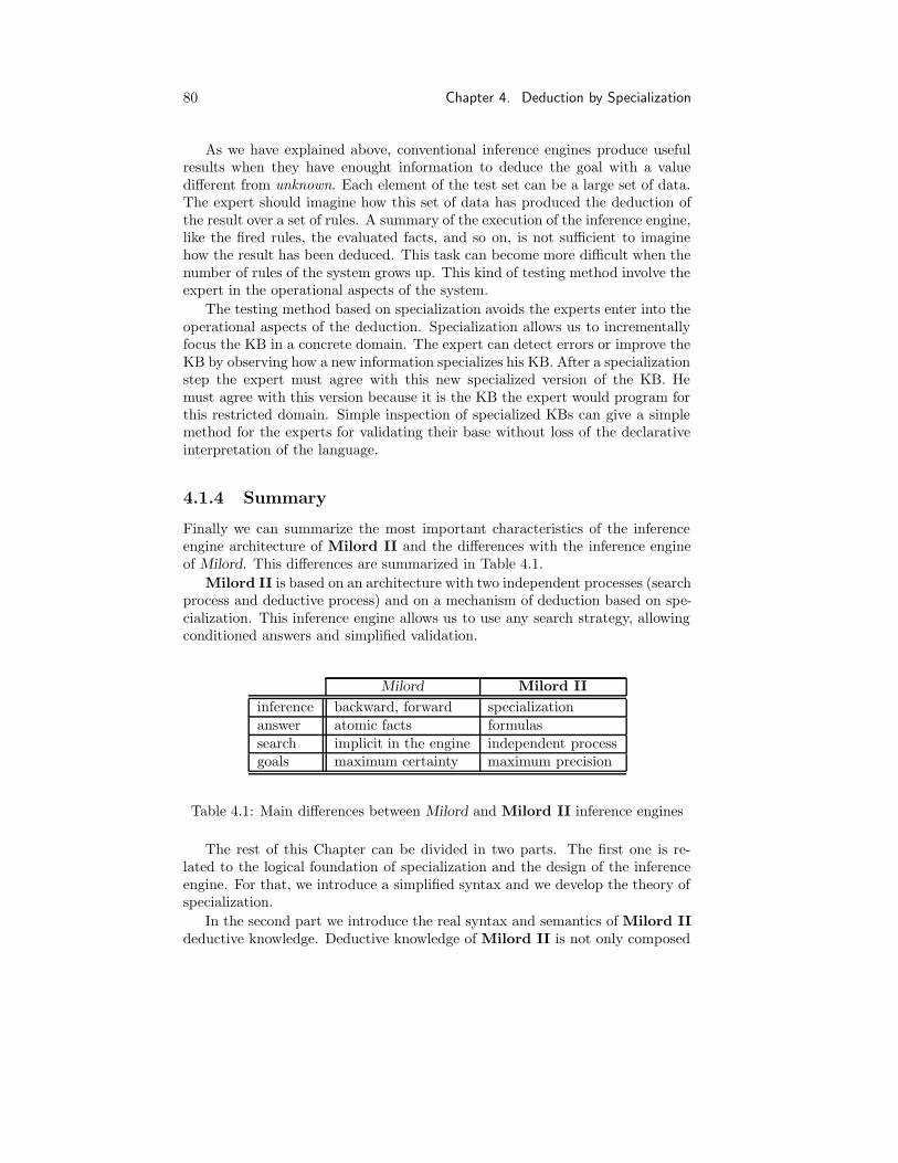
80 Chapter 4. Deduction by Specialization
As we have explained above, conventional inference engines produce usefulresults when they have enought information to deduce the goal with a valuedifferent from unknown. Each element of the test set can be a large set of data.The expert should imagine how this set of data has produced the deduction ofthe result over a set of rules. A summary of the execution of the inference engine,like the fired rules, the evaluated facts, and so on, is not sufficient to imaginehow the result has been deduced. This task can become more difficult when thenumber of rules of the system grows up. This kind of testing method involve theexpert in the operational aspects of the system.
The testing method based on specialization avoids the experts enter into theoperational aspects of the deduction. Specialization allows us to incrementallyfocus the KB in a concrete domain. The expert can detect errors or improve theKB by observing how a new information specializes his KB. After a specializationstep the expert must agree with this new specialized version of the KB. Hemust agree with this version because it is the KB the expert would program forthis restricted domain. Simple inspection of specialized KBs can give a simplemethod for the experts for validating their base without loss of the declarativeinterpretation of the language.
4.1.4 Summary
Finally we can summarize the most important characteristics of the inferenceengine architecture of Milord II and the differences with the inference engineof Milord. This differences are summarized in Table 4.1.
Milord II is based on an architecture with two independent processes (searchprocess and deductive process) and on a mechanism of deduction based on spe-cialization. This inference engine allows us to use any search strategy, allowingconditioned answers and simplified validation.
Milord Milord II
inference backward, forward specializationanswer atomic facts formulassearch implicit in the engine independent processgoals maximum certainty maximum precision
Table 4.1: Main differences between Milord and Milord II inference engines
The rest of this Chapter can be divided in two parts. The first one is re-lated to the logical foundation of specialization and the design of the inferenceengine. For that, we introduce a simplified syntax and we develop the theory ofspecialization.
In the second part we introduce the real syntax and semantics of Milord IIdeductive knowledge. Deductive knowledge of Milord II is not only composed

4.2. Specialization Calculus 81
of facts and rules. Practice in ES development has driven us to add a set ofextralogical components to the base language.
4.2 Specialization Calculus
Specialization Calculus is the key point of the deductive process used in Mi-lord II, and then of the whole behavior of the system. In this Section we givea formal description and study the properties of this calculus. Here we presentthe abstract syntax of the language, the semantics and a soundness theorem.Examples are written in real syntax, but they are easily understandable5. Thepurpose of the detailed examples is to introduce and acquire familiarity with thecalculus with intervals of truthvalues.
4.2.1 Syntax
Here we present a very simplified syntax of facts and rules for the deductiveknowledge of Milord II. It allows us to introduce formally the specializationcalculus. Afterwards we will present the concrete syntax which does not intro-duce significant changes in the theoretical results.
A propositional language Ln = (An, Σ, C,Sn) is defined by:
• The set of linguistic terms An as defined in Chapter 3.
• A signature Σ consisting on a set of atomic propositional symbols plus trueand false.
• A set of Connectives: C = ¬,∧,→
• A set of Sentences: Sn = Mv–Literals ∪ Mv–Rules
Sentences are pairs of classical–like propositional sentences and intervalsof truth–values. The classical–like propositional sentences are restricted tobe literals or rules. Thus, the sentences of the language are of the followingtypes:
Mv–Atoms: (p, V ) | p ∈ Σ and V ∈ Int(An)
Mv–Literals: (p, V ) | (p, V ) ∈ Mv–Atoms or p = ¬q and (q, V ) ∈ Mv–Atoms
Mv–Rules: (p1 ∧ p2 ∧ · · · ∧ pn → q, V ) | pi and q are literals, V = [a, 1]is an upper interval of Int(An) where a > 0, and ∀i, j(pi 6= pj , pi 6=¬pj , q 6= pj , q 6= ¬pj)
5The logic used in the examples of this chapter is the one defined in Chapter 3. Remem-ber that the linguistic terms are A5 = impossible, slightly possible, possible, very possible,definite.

82 Chapter 4. Deduction by Specialization
This syntax is close to the standard one in ESs, that is, facts and produc-tion rules. The most important difference is that facts and rules are weightedby intervals of truthvalues. The atomic symbols of the signature are what wecall facts in ES terminology. Rules are composed of a set of conditions and aconclusion. The conditions and the conclusion are facts or negations of facts.As usual, the facts contained in a rule only appear once, in the conditions or inthe conclusion.
In the next sections we will introduce the real syntax of facts and rules. Herewe limit our expansion to the logical components of deductive knowledge andwe will use the terminology introduced above.
The connectives are translated to the real syntax as: no (¬), and (∧), and if· · · then conclude (→). An example of rule in Milord II syntax is:
R005 If macrol and no (light seriousness) andentered to hospital then conclude no (roxi) is very possible
Notice that the symbol very possible after is represents the truthvalue of themv–rule. Only an element of An is introduced because the truthvalue of themv–rule is always implicitly considered an interval from an element of An to 1.We could say that this value represents the more pessimistic value of the rule.It is easy to see that the translation of the previous rule to the abstract syntaxis:
(macrol ∧ ¬light seriousness ∧ entered to hospital→ ¬roxi,[very possible,1])
There are two reasons to consider this kind of intervals for the conclusionsof rules. The first one is for simplicity. Despite the utility of using intervals oftruthvalues, experts express better their knowledge using only one value for therules. The second one is related to the semantics of specialization and it will beexplained in the next Section.
4.2.2 Semantics
After the description of the syntax of the abstract language, we present themeaning of the sentences introduced above. This allows us to give an interpre-tation of facts and rules with no ambiguity. It is very easy to missinterpret thelanguage as often do experts by translating the rules into natural language andincorporating all the ambiguities it has. Then it is mandatory the reference tothe exact meaning of the language.
Models
Models Mρ are defined by valuations ρ, i.e. mappings from the first componentsof sentences to An. The elementary case is the valuation of atomic symbols. Forinstance we can say that the fact macrol has the value possible, that is, ρ(macrol)= possible. From this elementary valuation and the operators Nn (negation),

4.2. Specialization Calculus 83
T (conjunction) and IT (implication) presented in Section 3.1 we can obtainvaluations of non atomic sentences.
Valuations of non atomic sentences as defined below hold that:
M1: ρ(¬p) = Nn(ρ(p))
M2: ρ(p1 ∧ p2) = T (ρ(p1), ρ(p2))
M3: ρ(p → q) = IT (ρ(p), ρ(q))
M4: ρ(true) = 1
M5: ρ(false) = 0
We can build an example with the facts and the rule given in the syntaxexample. Suppose that our model Mρ is:
ρ(macrol) = possibleρ(light seriousness) = impossibleρ(entered to hospital) = definiteρ(roxi) = slightly possible
We can extend the valuation function to the example rule as follows:
ρ(macrol ∧ ¬light seriousness ∧ entered to hospital → ¬roxi) =IT (T (ρ(macrol), T (Nn(ρ(light seriousness)), ρ(entered to hospital))),Nn(ρ(roxi))) =IT (T (possible, T (Nn(false), true)),Nn(slightly possible)) = definite
Satisfaction Relation
Given a model, that is, the valuations of facts and rules, we define when asentence is satisfied by a model. The satisfaction relation is defined as follows:
Definition 4.2 (Satisfaction Relation) The Satisfaction Relation between mod-els and sentences is defined by:
Mρ |= (p, V ) iff ρ(p) ∈ V
where V ∈ Int(An).
The satisfaction of a set of sentences is the satisfaction of each of them. Thissatisfaction relation introduces in our system the notion of imprecision presentedin Chapter 3, a sentence is satisfied if the valuation of the proposition belongsto an interval of truthvalues (it is not necessarily equal to a truthvalue). Forinstance we can show that the model above satisfies the rule given in the syntaxexample:
ρ(macrol) = possible, ρ(light seriousness) = impossible,ρ(entered to hospital) = definite, ρ(roxi) = slightly possible |=(macrol ∧ ¬light seriousness ∧ entered to hospital→ ¬roxi,[very possible,1])
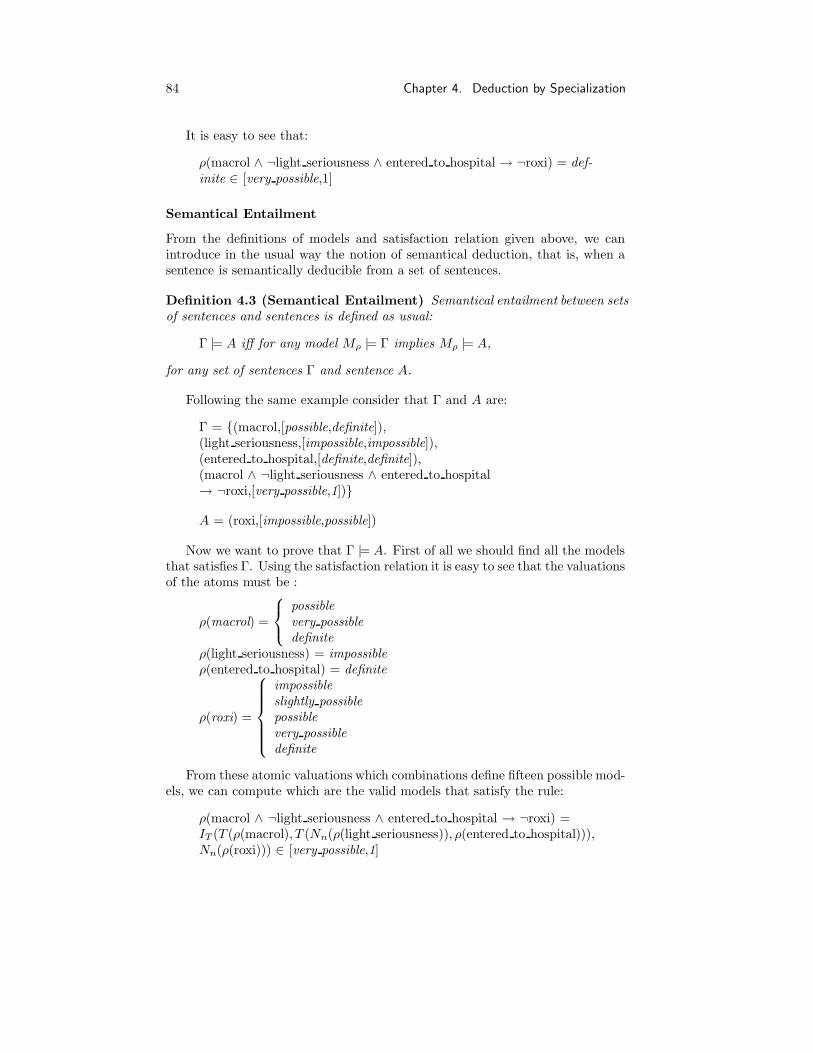
84 Chapter 4. Deduction by Specialization
It is easy to see that:
ρ(macrol ∧ ¬light seriousness ∧ entered to hospital → ¬roxi) = def-inite ∈ [very possible,1]
Semantical Entailment
From the definitions of models and satisfaction relation given above, we canintroduce in the usual way the notion of semantical deduction, that is, when asentence is semantically deducible from a set of sentences.
Definition 4.3 (Semantical Entailment) Semantical entailment between setsof sentences and sentences is defined as usual:
Γ |= A iff for any model Mρ |= Γ implies Mρ |= A,
for any set of sentences Γ and sentence A.
Following the same example consider that Γ and A are:
Γ = (macrol,[possible,definite]),(light seriousness,[impossible,impossible]),(entered to hospital,[definite,definite]),(macrol ∧ ¬light seriousness ∧ entered to hospital→ ¬roxi,[very possible,1])
A = (roxi,[impossible,possible])
Now we want to prove that Γ |= A. First of all we should find all the modelsthat satisfies Γ. Using the satisfaction relation it is easy to see that the valuationsof the atoms must be :
ρ(macrol) =
possiblevery possibledefinite
ρ(light seriousness) = impossibleρ(entered to hospital) = definite
ρ(roxi) =
impossibleslightly possiblepossiblevery possibledefinite
From these atomic valuations which combinations define fifteen possible mod-els, we can compute which are the valid models that satisfy the rule:
ρ(macrol ∧ ¬light seriousness ∧ entered to hospital → ¬roxi) =IT (T (ρ(macrol), T (Nn(ρ(light seriousness)), ρ(entered to hospital))),Nn(ρ(roxi))) ∈ [very possible,1]

4.2. Specialization Calculus 85
We can simplify the expression with the facts light seriousness and entered -to hospital that only can take a boolean value:
IT (ρ(macrol),Nn(ρ(roxi))) ∈ [very possible,1]
Using the Table 3.3 of the operator IT in this example, we can build theTable 4.2 that contains the valid models obtained.
ρ(light seriousness) ρ(entered to hospital) ρ(macrol) ρ(roxi)
impossible definite possible impossiblesli possiblepossible
very possible impossiblesli possiblepossible
definite impossiblesli possible
Table 4.2: Valid models of the example.
Then we have obtained eight models that satisfy Γ. It is easy to see that allthe valuations of roxi are in the interval [impossible,possible], so Γ entails A.
Now we are interested in semantical deduction. From mv–facts and mv–ruleswe want to obtain new mv–facts and specialized mv–rules. A set of interestingproperties of the semantic entailment that will play a major role in later proofsis presented next.
Proposition 4.1 If p, q, p1, . . . , pn denote literal symbols then the following prop-erties are fulfilled:
SR1: (p, V ) |= (p,W ) ⇔ V ⊆ W
SR2: (p, V ) |= (¬p,W ) ⇔ N ∗n(V ) ⊆ W
SR3: (p, V ), (p,W ) |= (p,U) ⇔ V ∩ W ⊆ U
SR4: (pi, Vi), (p1 ∧ · · · ∧ pn → q, V ) |= (p1∧· · ·∧pi−1∧pi+1∧· · ·∧pn → q,W ) ⇔MP ∗
T (Vi, V ) ⊆ W
SR5: MP ∗T (T ∗(V1, . . . , Vn),W ) =
MP ∗T (V1,MP ∗
T (V2, . . . ,MP ∗T (Vn,W ) . . .)), if W = [w, 1]
These properties6 give semantics to the negation of mv–atoms and the spe-cialization of mv–rules. The property SR5 is the justification of the equivalencewhich is the base of specialization (a ∧ b → c ≡ a → (b → c)). This is the otherreason cited above to use upper intervals in the mv–rules.
6The proof of these properties can be found in (Puyol et al., 1992c) and Appendix B.
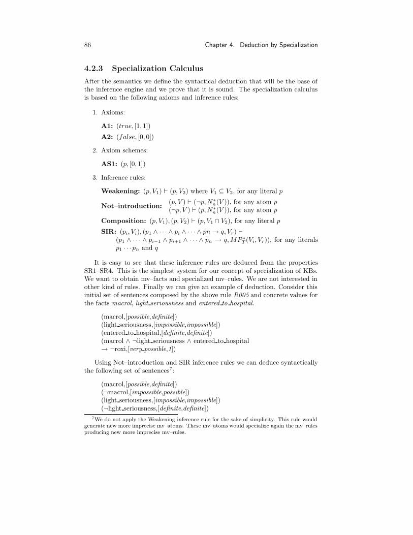
86 Chapter 4. Deduction by Specialization
4.2.3 Specialization Calculus
After the semantics we define the syntactical deduction that will be the base ofthe inference engine and we prove that it is sound. The specialization calculusis based on the following axioms and inference rules:
1. Axioms:
A1: (true, [1, 1])
A2: (false, [0, 0])
2. Axiom schemes:
AS1: (p, [0, 1])
3. Inference rules:
Weakening: (p, V1) ` (p, V2) where V1 ⊆ V2, for any literal p
Not–introduction:(p, V ) ` (¬p,N∗
n(V )), for any atom p(¬p, V ) ` (p,N∗
n(V )), for any atom p
Composition: (p, V1), (p, V2) ` (p, V1 ∩ V2), for any literal p
SIR: (pi, Vi), (p1 ∧ · · · ∧ pi ∧ · · · ∧ pn → q, Vr) `(p1 ∧ · · · ∧ pi−1 ∧ pi+1 ∧ · · · ∧ pn → q,MP ∗
T (Vi, Vr)), for any literalsp1 · · · pn and q
It is easy to see that these inference rules are deduced from the propertiesSR1–SR4. This is the simplest system for our concept of specialization of KBs.We want to obtain mv–facts and specialized mv–rules. We are not interested inother kind of rules. Finally we can give an example of deduction. Consider thisinitial set of sentences composed by the above rule R005 and concrete values forthe facts macrol, light seriousness and entered to hospital.
(macrol,[possible,definite])(light seriousness,[impossible,impossible])(entered to hospital,[definite,definite])(macrol ∧ ¬light seriousness ∧ entered to hospital→ ¬roxi,[very possible,1])
Using Not–introduction and SIR inference rules we can deduce syntacticallythe following set of sentences7:
(macrol,[possible,definite])(¬macrol,[impossible,possible])(light seriousness,[impossible,impossible])(¬light seriousness,[definite,definite])
7We do not apply the Weakening inference rule for the sake of simplicity. This rule wouldgenerate new more imprecise mv–atoms. These mv–atoms would specialize again the mv–rulesproducing new more imprecise mv–rules.

4.3. Implementation 87
(entered to hospital,[definite,definite])(¬entered to hospital,[impossible,impossible])(macrol ∧ ¬light seriousness ∧ entered to hospital→ ¬roxi,[very possible,1])(¬light seriousness ∧ entered to hospital → ¬roxi,[possible,1]))(entered to hospital → ¬roxi,[possible,1]))(¬roxi,[possible,1])(roxi,[impossible,possible])
For simplicity we have not written all the resultant sentences obtained fromthe application of weakening. Finally the conclusion is:
A = (roxi,[impossible,possible])
4.2.4 Soundness and Completeness
From properties SR1, SR2, SR3 and SR4 of the semantical entailment, it is easyto check that the above specialization calculus is sound.
Theorem 4.1 (Soundness) Let A be a sentence and Γ a set of sentences.Then Γ ` A implies Γ |= A
It is straightforward to see that our deductive system is not complete. Forinstance, we have (p → q, 1), (q → r, 1) |= (p → r, 1) but (p → q, 1), (q →r, 1) 6` (p → r, 1). It is also the case that the language is not complete for literaldeduction in general. For instance, we have (p → q, 1), (¬p → q, 1) |= (q, 1)but (p → q, 1), (¬p → q, 1) 6` (q, 1). However, it can be proved that the systemis complete for literal deduction in the context of a restricted language setting.Soundness and restricted completeness are proved in (Puyol et al., 1992c) andin Appendix B.
Despite our deductive system is not complete, we can show that it is usefulfor our purpose of obtaining specialization of KBs. We need to specialize a rulewhen we know the truthvalue of an atom that belongs to the premise of thatrule and in this case we have:
(p1, V1), (p1 ∧ · · · ∧ pn → q,W ) |= (p2 ∧ · · · ∧ pn → q, U) ⇔(p1, V1), (p1 ∧ · · · ∧ pn → q,W ) ` (p2 ∧ · · · ∧ pn → q, U)
To finish this part we introduce the implementation of that SpecializationCalculus.
4.3 Implementation
In the above Section we have introduced the Specialization Calculus used inMilord II. Axioms and inference rules are the sufficient mechanisms to dospecialization from the logic point of view. We have proved that the propertieswe were interested in hold. Now we want to implement that SpecializationCalculus.

88 Chapter 4. Deduction by Specialization
The requirements for the inference engine are closely related to the behaviorof the whole system. Remember that the specialization of deductive knowledgeis the base for users/system communication. Furthermore the inference enginemust also handle the control knowledge. In summary, the inference engine isa key part of the whole system Milord II. In this Section we will present therequirements of the inference engine and the concrete implementation.
4.3.1 Inference Engine Design
The simplest inference engine would be an inference engine that given a KB itwould apply all the inference rules of the Specialization Calculus until there isnot any rule that can be applied. In the last example we have showed this kindof behavior. But when we design the inference engine of Milord II we have newrequirements that determine which and when rules have to be applied.
In order to preserve the correctness of the inference engine with respect tothe semantics of Specialization Calculus, the inference engine does not introducehere extralogical components. The axioms and inference rules presented aboveare the only mechanisms to do specialization.
As usual we are interested in designing an efficient program but we do notmake a special point of this. Despite this we have introduced some control toimprove the efficiency of specialization.
Furthermore we should take into account that this inference engine must beintegrated in the whole system. Possible simplifications of the inference engineare not possible because we need to handle the actions of the local control ofa module (control will be explained in Chapter 5). The following are the moreimportant points that we take into account in the design of the inference engineof Milord II:
• The task of the inference engine is to produce specialization of deductiveknowledge. As seen in Section 4.1 the specialized deductive knowledge isused to present an enriched behavior of ESs. The internal representationof deductive knowledge should facilitate that task. We have chosen aninternal representation that it is close to our concept of specialization.
• When deducing facts we are only interested in values (intervals of truth–values) having maximum precision. Then the inference engine will assign adefinitive value to a fact when it is the most precise (you can find commentson imprecision and its control in Sections 3.2.2 and 5.1.2 respectively) thatwe can obtain from the deductive knowledge in the current case; otherwisethe values are considered to be provisional.
• The inference engine must be interleaved with control. Then it should fitthe actions made by the control. We avoid some simplifications that wouldproduce a more efficient inference engine because in the inference enginedesign we must foresee the actions of the control.
Following the above criteria of design now we will comment the use of theinference rules of the Specialization Calculus.

4.3. Implementation 89
The first point is that we want to obtain maximum precision. This impliesthat the inference engine must not use the Weakening inference rule that pro-duces valid but less precise values. Another consequence of maximum precisionis that the system specializes the mv–rules with the more precise mv–atoms.Then, it is not necessary to conserve the previous versions of the mv–rules be-cause the rules will not be specialized again with the same mv–atoms. Thisimplies the substitution of mv–rules with their specialized versions.
From the expert point of view a KB is represented by means of mv–rulesand mv–atoms. Specialization of a KB should conserve that representation asshown in the introduction of this Chapter. Then we are not interested in creatingmv–literals. Not–Introduction is only used when necessary to calculate the newtruthvalue of mv–rules or that of their conclusion when they are specialized.
Finally notice that Composition is used to calculate the truthvalue of a factwhen more that one rule conclude it. Each rule gives a provisional value to theconclusion. Finally the definitive value is obtained by means of Composition.
Following this requirements we will define the inference engine. We will usefunctional and algorithmic descriptions. We use a simple example to illustratethe behavior of the inference engine. First of all we introduce the internal datastructure of a KB.
4.3.2 Internal Representation of Deductive Knowledge
Here we present the internal representation of deductive knowledge to make clearwhat is the task of the inference engine and what are the entries to control.
We are not interested in maintaining a data structure composed of facts andrules. We propose a new data representation that it is very close to the realimplementation and that clarifies control and extralogical components of theinference engine.
We maintain the above definitions for mv–atoms, and mv–literals, but wepropose a new representation of mv–rules that allows us to make easy the func-tional descriptions by means of set operations.
Definition 4.4 (Mv–Rule) A mv–rule is represented as a 3–tupler = (mr, cr, ρr) where mr is the premise (a set of literals), cr is the conclusion(a literal) and ρr is the truthvalue of the rule (an interval of truthvalues suchthat ρr = [α, 1] and α ∈ An).
For instance the mv–rule (c ∧ d → e,[ρ2,1]) can be represented as the 3–tuple: (c, d, e, [ρ2, 1]). From that we can give the definition of a knowledgebase. Given a set of mv–rules, it consists in associating each atom appearing inthe mv–rules with its current truth–value (provisional or definitive one) and themv–rules that can deduce it, that is, those whose conclusion is that atom or thenegation of that atom. In the following we will call knowledge base the internalrepresentation of the deductive knowledge.
Definition 4.5 (Knowledge Base) Let R be a set of mv–rules and let FR bethe set of all atoms appearing in the rules of R. We define a knowledge base

90 Chapter 4. Deduction by Specialization
KBR as a mapping8:
KBR : FR → Int(An) ×P(R)
where, for each f ∈ FR, KBR(f) = (vf , Rf ), being Rf = r ∈ R|r = (mr, cr , ρr)and cr = f or cr = ¬f
Initially we build a knowledge base with truthvalues of the atoms [0, 1]. Itmeans that the atoms initially has the most imprecise value. Notice that a KBwith all the atoms with truthvalues [0, 1] is always consistent in our specializa-tion calculus (axiom scheme AS2). The truthvalues of atoms can be changedby the rules that deduce them (giving a more precise truthvalue by means ofComposition inference rule) or by external valuations of atoms. The truthvalueof an atom is considered to be provisional when there are rules that can concludeit; otherwise it is considered to be definitive.
Now we can see an example of initial KB. Suppose that we have a deductiveknowledge composed of the following set of mv–rules:
R = (a ∧ b → c,[ρ1,1]), (a ∧ f → ¬ c,[ρ2,1]), (c ∧ d → e,[ρ3,1])
It is easy to see that the set FR is:
FR = (a, b, c, d, e, f)
Now we can translate the example to the new representation. We create atable (mapping) from atoms of FR to its initial truthvalue ([0,1]) and the set ofmv–rules that deduce them. Then the knowledge base is the mapping KB suchthat:
KB(a) = ([0 , 1 ], ∅)KB(b) = ([0 , 1 ], ∅)KB(c) = ([0 , 1 ], (a, b, c, [ρ1, 1]), (a, f,¬c, [ρ2, 1]))KB(d) = ([0 , 1 ], ∅)KB(e) = ([0 , 1 ], (c, d, e, [ρ3, 1]))KB(f) = ([0 , 1 ], ∅)
Now we will define the specialization of KBs represented by the above for-malism. We will use the same example to illustrate the explanation.
4.3.3 Specialization
First of all we give a functional description of specialization of mv–rules. Givinga mv–rule and a mv–atom, the mapping SR will specialize the mv–rule withrespect of that mv–atom. It will return the new specialized mv–rule, or a newmv–atom in the case that the initial mv–rule would be able to deduce its con-clusion.
8P(R) is the powerset of the set R.

4.3. Implementation 91
Definition 4.6 (Specialization of Mv–Rules) Let R be a set of mv–rulesand F ∗ a set of mv–atoms F ∗ = (p, ρp)|p ∈ FR. We define SR as a mapping:
SR : R × F ∗ → R × F ∗
SR(r, (p, ρp)) =
(r, (∅, [0, 1])) if p 6∈ mr and ¬p 6∈ mr
(r′, (∅, [0, 1])) if p ∈ mr or ¬p ∈ mr
(∅, (q, α)) if mr = p or mr = ¬pand cr = q or cr = ¬q
where
r′ =
(mr − p, cr ,MP ∗T (ρp, ρr)) if p ∈ mr
(mr − ¬p, cr ,MP ∗T (N∗
n(ρp), ρr)) if ¬p ∈ mr
and
α =
MP ∗T (ρp, ρr) if mr = p and cr = q
N∗n(MP ∗
T (ρp, ρr)) if mr = ¬p and cr = qMP ∗
T (N∗n(ρp), ρr) if mr = p and cr = ¬q
N∗n(MP ∗
T (N∗n(ρp), ρr)) if mr = ¬p and cr = ¬q
Negations of mv–atoms are calculated by means of the Not–introductioninference rule, and the specialization of mv–rules is done using SIR inferencerule. Notice that we only generate mv–atoms. Taking again the same examplewe can do the specialization of the mv–rule of the last example obtaining a newspecialized mv–rule:
SR((a, f, ¬ c,[ρ2,1]), (f,[ρ4, ρ′4]) =
((a, ¬ c,[MPT (ρ4, ρ2),1]), ∅)
If we specialize again the rule we obtain a mv–atom:
SR((a, ¬ c,[MPT (ρ4, ρ2),1]), (a,[ρ5, ρ′5]) =
(∅, (c, N ∗n(MP ∗
T ([MPT (ρ4, ρ2), 1], [ρ5, ρ′5]))))
After the definition of rule specialization we can explain atom specialization.A kb–atom is a structure that associates to an atom its truthvalue and therules that conclude it. Then, atom specialization will modify the structure of akb–atom with a mv–atom.
First of all we find a mv–rule from the set of mv–rules that conclude the atomsuch that it can be specialized with respect to that mv–atom. If no rule of thistype can be found the specialization of the kb–atom returns the same structure.Otherwise it returns a new specialized rule (r ′ 6= r) or a new mv–atom (r = ∅).If the specialization of a rule returns a new rule (SR(r, f∗) = (r′, (∅, [0, 1]))) thenwe substitute the rule by the specialized one and the truthvalue is not changed.Notice that [a, b] ∩ [0, 1] = [a, b]. If it returns a new mv–atom (SR(r, f∗) =(∅, (p′, v′))) the rule is eliminated and the new truthvalue is calculated by meansof the Composition inference rule.
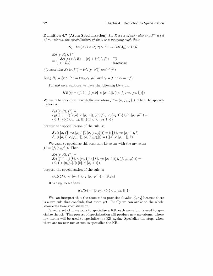
92 Chapter 4. Deduction by Specialization
Definition 4.7 (Atom Specialization) Let R a set of mv–rules and F ∗ a setof mv–atoms, the specialization of facts is a mapping such that:
SC : Int(An) ×P(R) × F ∗ → Int(An) ×P(R)
SC((v,Rf ), f ∗)
=
SC((v ∩ v′, Rf − r + r′), f ∗) (*)(v,Rf ) otherwise
(*) such that SR(r, f∗) = (r′, (p′, v′)) and r′ 6= r
being Rf = r ∈ R|r = (mr, cr, ρr) and cr = f or cr = ¬f
For instance, suppose we have the following kb–atom:
KB(c) = ([0, 1], (a, b, c, [ρ1, 1]), (a, f,¬c, [ρ2, 1]))
We want to specialize it with the mv–atom f ∗ = (a, [ρ5, ρ′5]). Then the special-
ization is:
SC((v,R), f ∗) =SC(([0, 1], (a, b, c, [ρ1, 1]), (a, f,¬c, [ρ2, 1])), (a, [ρ5, ρ′
5])) =([0, 1], (b, c, [ρ6, 1]), (f,¬c, [ρ7, 1]))
because the specialization of the rule is:
SR((a, f,¬c, [ρ2, 1]), (a, [ρ5, ρ′5])) = ((f,¬c, [ρ6, 1]), ∅)
SR((a, b, c, [ρ1, 1]), (a, [ρ5, ρ′5])) = ((b, c, [ρ7, 1]), ∅)
We want to specialize this resultant kb–atom with the mv–atomf∗ = (f, [ρ4, ρ
′4]). Then
SC((v,R), f ∗) =SC(([0, 1], (b, c, [ρ6, 1]), (f,¬c, [ρ7, 1])), (f, [ρ4, ρ′
4])) =([0, 1] ∩ [0, ρ8], (b, c, [ρ6, 1]))
because the specialization of the rule is:
SR((f,¬c, [ρ3, 1]), (f, [ρ4, ρ′4])) = (∅, ρ8)
It is easy to see that:
KB(c) = ([0, ρ8], (b, c, [ρ6, 1]))
We can interpret that the atom c has provisional value [0, ρ8] because thereis a mv–rule that conclude that atom yet. Finally we can arrive to the wholeknowledge base specialization:
Given a set of mv–atoms to specialize a KB, each mv–atom is used to spe-cialize the KB. This process of specialization will produce new mv–atoms. Thesemv–atoms will be used to specialize the KB again. Specialization stops whenthere are no new mv–atoms to specialize the KB.

4.3. Implementation 93
Definition 4.8 (KB Specialization) Let KB be a set of knowledge bases andF ∗ a set of mv–atoms such that F ∗ = (p, V )|p ∈ FR. KB specialization isdefined as a mapping:
SKB : KB ×P(F ∗) → KB
SKB(kb, F ∗) =
SKB(kb′, F ∗ − f∗ + F ∗′
) if F ∗ 6= ∅kb otherwise
where ∀fkb ∈ FR,
kb′(fkb) =
(v, ∅) if (fkb, v) = f ∗ or kb(fkb) = (v, ∅)SC(kb(fkb), f ∗) otherwise
and
F ∗′
= y = (p, ρy)|kb(p) = (v,R),SC(kb(p), f ∗) = (ρy, ∅), p ∈ FR
Finally we can see the last example consisting in specializing the last KBwith the atom b.
SKB(kb, (b, ρ10)) = SKB(kb′, F ∗)
where f ∗ = (b, ρ10)
KB′(a) = (ρ5, ∅)KB′(b) = ([0 , 1 ], ∅)KB′(c) = SC((ρ9, (b, c, [ρ1, 1])), (b, ρ10)) = (ρ11, ∅))KB′(d) = ([0 , 1 ], ∅)KB′(e) = SC(([0, 1], (c, d, e, [ρ2, 1])), (b, ρ10)) =([0, 1], (c, d, e, [ρ2, 1]))KB′(f) = (ρ7, ∅)
F ∗ = (c, ρ11)
Finally
KB′′(a) = (ρ5, ∅)KB′′(b) = ([0, 1], ∅)KB′′(c) = (ρ11, ∅)KB′′(d) = ([0, 1], ∅)KB′′(e) = ([0, 1], (d, e, [ρ12, 1]))KB′′(f) = (ρ7, ∅)
We have seen the specialization calculus and the concrete implementationby the above description of the inference engine function SKB. This inferenceengine has been designed avoiding extralogical components and then assuring thecorrectness of the inference engine with respect to the semantics of specializationcalculus. In Chapter 5 we will enrich the inference engine with the actions ofcontrol.
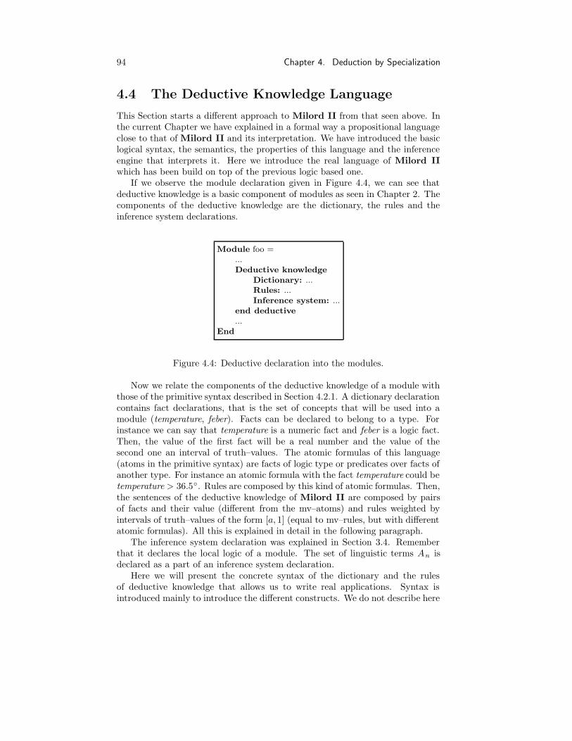
94 Chapter 4. Deduction by Specialization
4.4 The Deductive Knowledge Language
This Section starts a different approach to Milord II from that seen above. Inthe current Chapter we have explained in a formal way a propositional languageclose to that of Milord II and its interpretation. We have introduced the basiclogical syntax, the semantics, the properties of this language and the inferenceengine that interprets it. Here we introduce the real language of Milord IIwhich has been build on top of the previous logic based one.
If we observe the module declaration given in Figure 4.4, we can see thatdeductive knowledge is a basic component of modules as seen in Chapter 2. Thecomponents of the deductive knowledge are the dictionary, the rules and theinference system declarations.
Module foo =...Deductive knowledge
Dictionary: ...Rules: ...Inference system: ...
end deductive
...End
Figure 4.4: Deductive declaration into the modules.
Now we relate the components of the deductive knowledge of a module withthose of the primitive syntax described in Section 4.2.1. A dictionary declarationcontains fact declarations, that is the set of concepts that will be used into amodule (temperature, feber). Facts can be declared to belong to a type. Forinstance we can say that temperature is a numeric fact and feber is a logic fact.Then, the value of the first fact will be a real number and the value of thesecond one an interval of truth–values. The atomic formulas of this language(atoms in the primitive syntax) are facts of logic type or predicates over facts ofanother type. For instance an atomic formula with the fact temperature could betemperature > 36.5. Rules are composed by this kind of atomic formulas. Then,the sentences of the deductive knowledge of Milord II are composed by pairsof facts and their value (different from the mv–atoms) and rules weighted byintervals of truth–values of the form [a, 1] (equal to mv–rules, but with differentatomic formulas). All this is explained in detail in the following paragraph.
The inference system declaration was explained in Section 3.4. Rememberthat it declares the local logic of a module. The set of linguistic terms An isdeclared as a part of an inference system declaration.
Here we will present the concrete syntax of the dictionary and the rulesof deductive knowledge that allows us to write real applications. Syntax isintroduced mainly to introduce the different constructs. We do not describe here

4.4. The Deductive Knowledge Language 95
all the possible syntactical forms that are valid in the language. Please referencethe complete syntax in Appendix A. When possible we use real examples toillustrate the programming task with Milord II.
4.4.1 Facts
Facts are one of the most primitive components of the language Milord II. Theyare atomic symbols that represent the concepts that will be used in a module.Facts can be observable (fever), deducible (pneumonia) and so on.
The declaration of a fact is composed by an atomic name that is the identi-fication of the fact and a set of attributes: name, question, type, function andrelations. Facts can be referenced inside a module9, for instance in its rules.
Facts are declared in dictionary declarations. An example of dictionary isgiven in Figure 4.5. It contains type and fact (predicate) declarations. In thisexample we can see the declaration of a fact identified by assoc treat.
Dictionary:
Types: farmac = (carbamacepina, teofilina, digoxina,dicumarinics, ciclosporina,difenilhidantoina)
Predicates:
assoc treat=Name: ”Associated Treatments”Question: ”which farmacs the patient takes usually?”Type: farmacRelation: needs true use farmacs?
Figure 4.5: Example of dictionary declaration
Attributes of Facts
Here we will describe all the attributes that facts have. Name and type attributesof facts are mandatory.
Name: This is an attribute that associates a long name to the fact. Expertsuse atomic short names to identify a fact mainly to simplify the rulesand metarules. The long name is presented to the user for helping itsunderstanding of the concept the fact represents.
Question: This is the text of the question made to the user when a fact belongsto the import interface. When the system asks a question to the user itpresents the long name of the fact, the question and the set of possible
9A module can reference all the facts declared into the module. Facts declared into othermodules can be referenced by using a path name if they are accessible (remember that theycan be hidden by the information hiding mechanism).

96 Chapter 4. Deduction by Specialization
answers among which the user can select. When a fact belongs to theimport interface of a module this attribute is mandatory.
Type: It declares the type of the fact. The type of a fact is the set of values thatit can take when it is evaluated. There are five predefined types, that is,boolean, logic, numeric, array and class; and one user–defined type namedenumerated. A fact can be evaluated over the set of values determined byits type.
Function: Sometimes we want to evaluate a fact with a procedural form in-stead of a deductive one. This allows us to evaluate a fact by means of afunctional description.
Relation: It stablishes named relations with another facts. This implements adirected graph of relations among facts that can be used to classify facts,to stablish an order of evaluation, etc.
We can see the example in Figure 4.5. This fact has a name, a questionbecause its value will be obtained from the user, and the type (declared inthe type declaration of the dictionary) which is a set of farmacs. The relationdeclaration means that the fact use farmacs? needs to be known true to givesense to the fact assoc treat.
After this summary description of the attributes of facts, we will explain indetail the type, function and relations attributes.
Types of facts
In the first part of this Chapter we have worked with facts weighted by anintervals of truthvalues. Now we say that this kind of facts are of logic type. Weneed to add more types that the logic one. We follow Milord in this but withsome variations. There are five predefined types: boolean, logic, numeric, arrayand class. The user can define new types of facts by enumeration, then we saythat facts are of order 0+. Here there is a summary of the types of Milord IIfacts:
Boolean: Are facts whose value can be Yes (true) or No (false). They areused when we want talk about the presence or absence of a concept. Forinstance we can consider that the fact has fever is a boolean fact becausewe have a criteria to decide if it is true or not the patient has fever.
Logic: The values of this facts are intervals10 of a set of linguistic terms thatrepresents uncertainty values. This set of terms must be defined in theinference system declaration (see Section 3.4). The kind of concepts thatcan be considered logic facts are those whose truthness can be valued,because there are subjective. For instance if we use a subjective criteria to
10Milord used only one element of a set of linguistic terms. This type of facts was named
fuzzy.

4.4. The Deductive Knowledge Language 97
appreciate if a patient has fever as touching with the hand, we can considerthat the fact has fever is a logic fact (we can say that has fever is possible).
Numeric: The value is an interval of real numbers. They are used in quantita-tive data, for instance temperature, number of leucocits, etc.
Enumerated: This is the only type that can be defined by the user. This type isa set of symbolic values. The value of a fact of enumerated type is a subsetof the type declaration, or none. A difference with the enumerated typein Milord is that each symbol of a enumerated fact has a certainty valueassociated (it is a fuzzy set as shown in Section 3.2.3). In Figure 4.5 we cansee an example of enumerated type declaration farmac. An enumeratedtype can be defined in the type attribute of a fact declaration. It can alsobe defined in the type declaration of the dictionary (see Figure 4.5) andgive it a name. This name can be used to declare a type of a fact.
Array: The value of this kind of facts are arrays of real numbers of any dimen-sion. This is a special type of fact and it is only used in an example ofbelief propagation application described in the Section 6.6.
Class: The facts of this type have no value. They are used only to definerelations with other facts. For instance we can consider that the fact oralis a class fact because we want to define a relation with it in the declarationof the antibiotics that are administrated orally.
The facts that belong to the import interface of a module can be asked to theuser11. He can answer with the set of values that are allowed depending of thetype of the fact. Users are able to answer unknown to a system question. It isvery important to distinguish this answer of the interval [0, 1]. In the first casethe system considers that the fact questioned provisionally has no value. Then,it do not produce any actions on the module, it is not used to specialize the KB.The interval [0, 1] is an interval of truth–values used internally that representsthe definitive value unknown.
Fact Functions
Fact functions allows us to implement a set of functionalities that are useful inthe practice of ESs. Here we emphasize possible applications of functions asinterfaces with other programs, procedural evaluations of facts and fuzzy sets.
The function attribute of a fact is programmed in Common Lisp12. It isa lambda–expression without parameters. This lambda–expression is consideredto be into a lexical closure that contains the name of the facts declared into amodule. The evaluation of these fact names returns their value. Then the body
11Facts of the import interface are not always asked to the user. In some cases the controlof the module can give a value to an imported fact before asking it to the user.
12Underline language of Milord II is Common Lisp, then it is easy to introduce part of theES programmed in this language. In this Section we will use Common Lisp terminology thatis considered to be well known. Details of this can be found in (Steele, 1984).

98 Chapter 4. Deduction by Specialization
of the lambda–expression can contain fact names and they will be substitutedby their values.
The value of a fact that contains a function attribute in its declaration iscalculated by means of the evaluation of that function. To evaluate this kindof fact its function attribute is evaluated and the result of this evaluation isattached to the fact. Now we can see a set of examples of the function attribute.
One of the characteristics of Milord II commented in the introduction isthat it should work in a realistic computer environment. Function attributes canprovide a tool for communicating an ES with other programs. For instance inSpong–IA application the system asks the user which is the form of the spongehe wants to classify. Then it is more clear if the question is joined with a setof pictures representing the possible forms. The user can select one of themby means of a picture representation program. For instance, the evaluation ofthe fact form can be obtained by means of a function that uses that program.Function attributes can be used as a sort of interface with other programs asgraphics, databases, etc.
Sometimes the value of a fact can be obtained easily by means of a mathe-matical expression or a procedure. An example of function attribute of Terap–IA
application can be seen in Figure 4.6. The value of the fact clearance of creatinincan be obtained by means of the following expression. In Figure 4.6 we can seethe declaration of this fact creat clear that contains a function attribute.
clearance of creatinin = 140 −
age × weight ×
1.0 if male0.8 if female
72
Creat clear=Name: ”Clearance of creatinin”Type: numeric
Function:
#’(lambda ( )(- 140(/
(* age weight (case sex(male 1.0)(female 0.8)))
72)))
Figure 4.6: Example of function attribute
Another use of the function attribute of a fact is for declaring the charac-teristic function of a fuzzy set (see Section 3.2.3). In Figure 4.7 we can see anexample of fact declaration of the concept tall. This concept is represented by afuzzy set and declared with a function that given an interval of numeric values
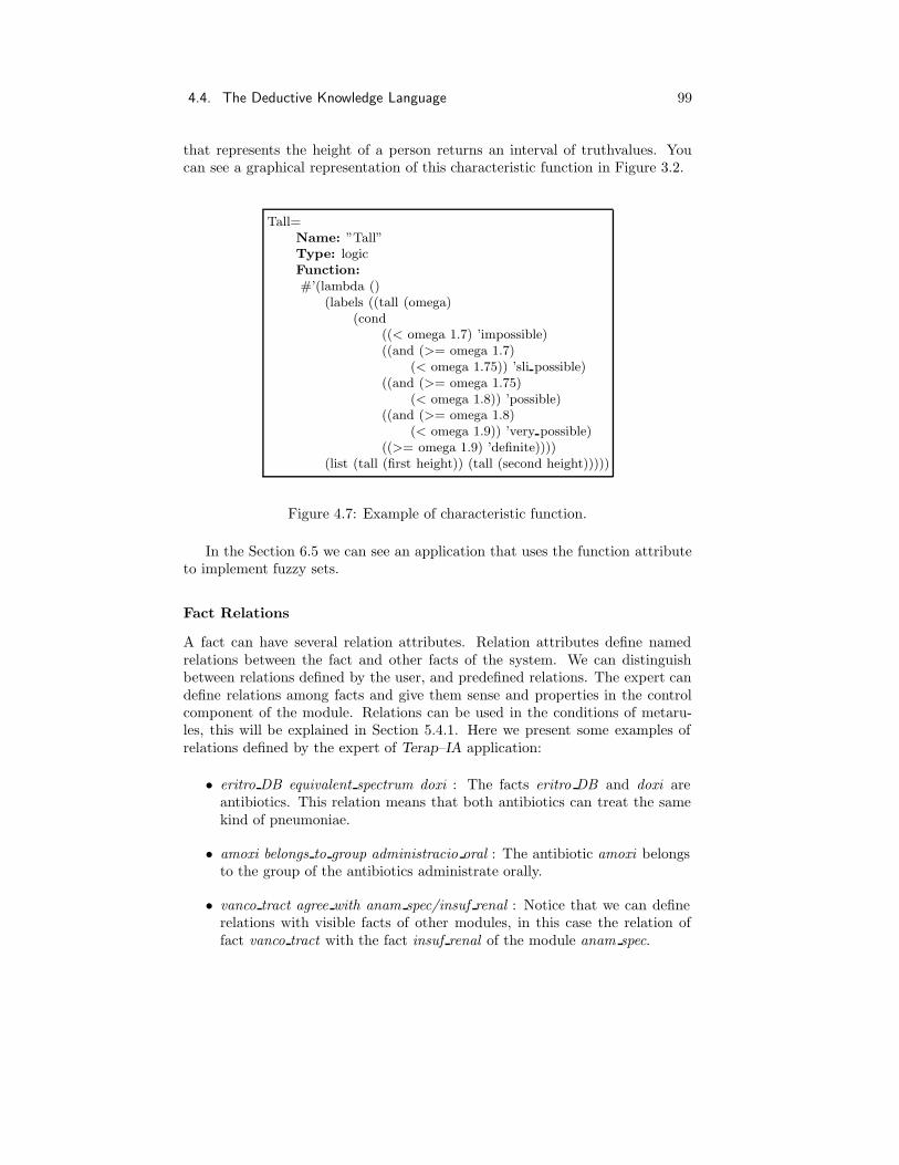
4.4. The Deductive Knowledge Language 99
that represents the height of a person returns an interval of truthvalues. Youcan see a graphical representation of this characteristic function in Figure 3.2.
Tall=Name: ”Tall”Type: logicFunction:
#’(lambda ()(labels ((tall (omega)
(cond((< omega 1.7) ’impossible)((and (>= omega 1.7)
(< omega 1.75)) ’sli possible)((and (>= omega 1.75)
(< omega 1.8)) ’possible)((and (>= omega 1.8)
(< omega 1.9)) ’very possible)((>= omega 1.9) ’definite))))
(list (tall (first height)) (tall (second height)))))
Figure 4.7: Example of characteristic function.
In the Section 6.5 we can see an application that uses the function attributeto implement fuzzy sets.
Fact Relations
A fact can have several relation attributes. Relation attributes define namedrelations between the fact and other facts of the system. We can distinguishbetween relations defined by the user, and predefined relations. The expert candefine relations among facts and give them sense and properties in the controlcomponent of the module. Relations can be used in the conditions of metaru-les, this will be explained in Section 5.4.1. Here we present some examples ofrelations defined by the expert of Terap–IA application:
• eritro DB equivalent spectrum doxi : The facts eritro DB and doxi areantibiotics. This relation means that both antibiotics can treat the samekind of pneumoniae.
• amoxi belongs to group administracio oral : The antibiotic amoxi belongsto the group of the antibiotics administrate orally.
• vanco tract agree with anam spec/insuf renal : Notice that we can definerelations with visible facts of other modules, in this case the relation offact vanco tract with the fact insuf renal of the module anam spec.
100 Chapter 4. Deduction by Specialization
There are a set of common problems faced by experts that can be solvedusing relations. Predefined relations are a set of relations with a global meaningin the system.
Belongs to: Experts usually use a belonging relation in their applications. Thisis a predefinited relation to avoid defining its transitive property, giving amore efficient system. For instance when the expert defines these three re-lations among antibiotics, doxi belongs to ABS/tetras 2, doxi DI belongs toABS/tetras 2 and tetras 2 belongs to tetraciclines, the system adds the newrelations doxi belongs to tetraciclines and doxi DI belongs to tetraciclines.
The relations of type needs are used to give a correct ordering of questionsto the user in the case of importable facts.
Needs: When the system is going to ask for the value of a fact, and this facthas a needs relation with another fact, this last fact will be asked first.For instance the relation pregnant needs sex means that before asking if aperson is pregnant the system will ask for his sex.
Needs true: This case is similar to the last one but the behavior is differentdepending on the answer of the first question. Consider the following ex-ample of relation from Spong–IA, organization needs true foreign. The firstquestion to the user would be if the sponge is foreign. If the user answers”yes”, the question organization would be asked. If the user answers ”no”,then the fact organization would become false and no question about itwould be made.
Needs false: The only difference with the last case is that the behavior is theinverse one with respect to the answer to the first question.
The needs relation work with importable facts of type boolean logic or enu-merated. In the case of enumerated facts we consider that false is the noneanswer and that true is any answer but none.
If the expression has the value unknown, then the fact takes the value un-known. If the expression is evaluated with false in the case of boolean and logicfacts, and with none in the case of enumerated facts, then the fact takes thesame value depending on the type of the fact.
Facts can be evaluated by the user (importable facts) , by the function at-tribute, or deduced by the rules. Before the above evaluation of a fact all theneeds relations are solved.
4.4.2 Rules
Syntax of Milord II rules is given in Figure 4.8. It is not necessary to give acomplete explanation of rules because they are similar to the mv–rules describedbefore. The only difference is that the conditions of rules can be composed ofpredicates on the facts of different type (conditions in mv–rules were literals oftype logic).
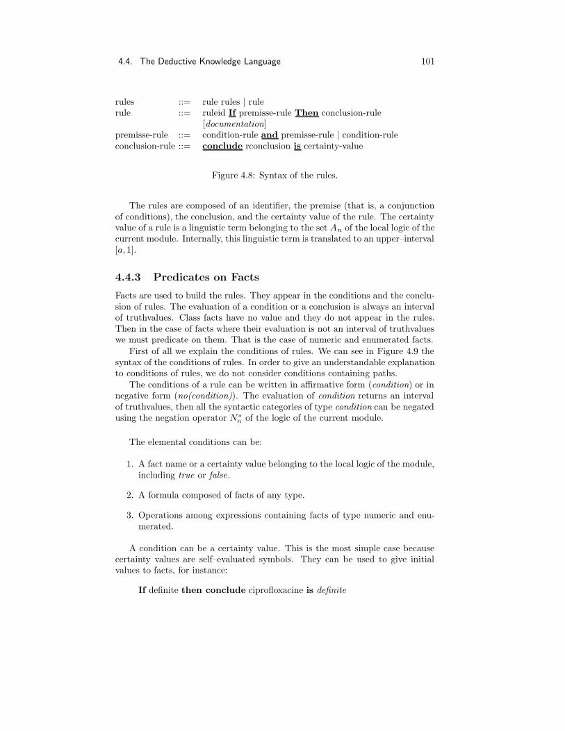
4.4. The Deductive Knowledge Language 101
rules ::= rule rules | rulerule ::= ruleid If premisse-rule Then conclusion-rule
[documentation]premisse-rule ::= condition-rule and premisse-rule | condition-ruleconclusion-rule ::= conclude rconclusion is certainty-value
Figure 4.8: Syntax of the rules.
The rules are composed of an identifier, the premise (that is, a conjunctionof conditions), the conclusion, and the certainty value of the rule. The certaintyvalue of a rule is a linguistic term belonging to the set An of the local logic of thecurrent module. Internally, this linguistic term is translated to an upper–interval[a, 1].
4.4.3 Predicates on Facts
Facts are used to build the rules. They appear in the conditions and the conclu-sion of rules. The evaluation of a condition or a conclusion is always an intervalof truthvalues. Class facts have no value and they do not appear in the rules.Then in the case of facts where their evaluation is not an interval of truthvalueswe must predicate on them. That is the case of numeric and enumerated facts.
First of all we explain the conditions of rules. We can see in Figure 4.9 thesyntax of the conditions of rules. In order to give an understandable explanationto conditions of rules, we do not consider conditions containing paths.
The conditions of a rule can be written in affirmative form (condition) or innegative form (no(condition)). The evaluation of condition returns an intervalof truthvalues, then all the syntactic categories of type condition can be negatedusing the negation operator N∗
n of the logic of the current module.
The elemental conditions can be:
1. A fact name or a certainty value belonging to the local logic of the module,including true or false.
2. A formula composed of facts of any type.
3. Operations among expressions containing facts of type numeric and enu-merated.
A condition can be a certainty value. This is the most simple case becausecertainty values are self–evaluated symbols. They can be used to give initialvalues to facts, for instance:
If definite then conclude ciprofloxacine is definite

102 Chapter 4. Deduction by Specialization
condition-rule ::= condition | no (condition )
condition ::= certainty-value |pathform |operator (expression, expression )
pathform ::= pathform-s | pathform-cpathform-s ::= predid | amodid/pathform-s
pathform-c ::= (formula )| amodid/pathform-c
formula ::= (pathform op pathform )
operator ::= < | > | <= | >= | = | /= | int
expression ::= number |operator-arit (expression, expression )|
operator-set (expression )|
pathform-s |(values )
values ::= values-crisp | values-fuzzyvalues-crisp ::= symbol , values | symbolvalues-fuzzy ::= (symbol , symbol ), values-fuzzy |
(symbol , symbol )
operator-arit ::= + | - | * | :operator-set ::= cut | core | support | complementop ::= plus
Figure 4.9: Syntax of the conditions of rules.
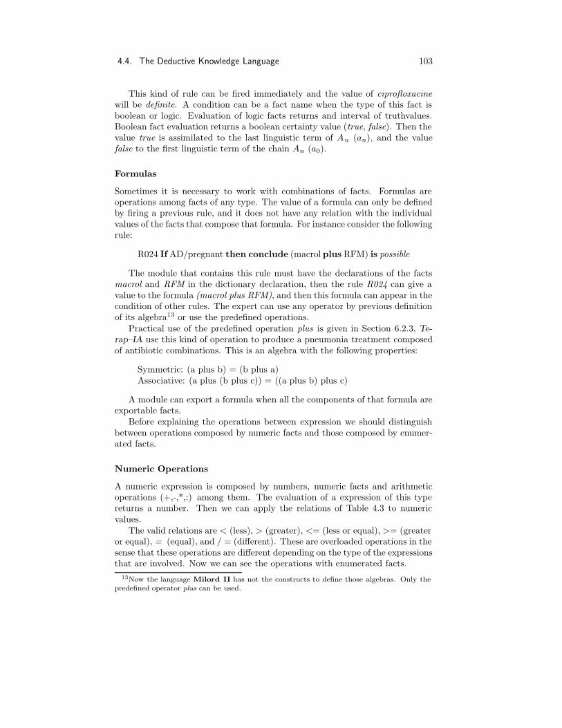
4.4. The Deductive Knowledge Language 103
This kind of rule can be fired immediately and the value of ciprofloxacinewill be definite. A condition can be a fact name when the type of this fact isboolean or logic. Evaluation of logic facts returns and interval of truthvalues.Boolean fact evaluation returns a boolean certainty value (true, false). Then thevalue true is assimilated to the last linguistic term of An (an), and the valuefalse to the first linguistic term of the chain An (a0).
Formulas
Sometimes it is necessary to work with combinations of facts. Formulas areoperations among facts of any type. The value of a formula can only be definedby firing a previous rule, and it does not have any relation with the individualvalues of the facts that compose that formula. For instance consider the followingrule:
R024 If AD/pregnant then conclude (macrol plus RFM) is possible
The module that contains this rule must have the declarations of the factsmacrol and RFM in the dictionary declaration, then the rule R024 can give avalue to the formula (macrol plus RFM), and then this formula can appear in thecondition of other rules. The expert can use any operator by previous definitionof its algebra13 or use the predefined operations.
Practical use of the predefined operation plus is given in Section 6.2.3, Te-
rap–IA use this kind of operation to produce a pneumonia treatment composedof antibiotic combinations. This is an algebra with the following properties:
Symmetric: (a plus b) = (b plus a)Associative: (a plus (b plus c)) = ((a plus b) plus c)
A module can export a formula when all the components of that formula areexportable facts.
Before explaining the operations between expression we should distinguishbetween operations composed by numeric facts and those composed by enumer-ated facts.
Numeric Operations
A numeric expression is composed by numbers, numeric facts and arithmeticoperations (+,-,*,:) among them. The evaluation of a expression of this typereturns a number. Then we can apply the relations of Table 4.3 to numericvalues.
The valid relations are < (less), > (greater), <= (less or equal), >= (greateror equal), = (equal), and / = (different). These are overloaded operations in thesense that these operations are different depending on the type of the expressionsthat are involved. Now we can see the operations with enumerated facts.
13Now the language Milord II has not the constructs to define those algebras. Only thepredefined operator plus can be used.

104 Chapter 4. Deduction by Specialization
Enumerated Operations
Remember the example in Figure 4.5. The enumerated fact is a fuzzy set namedassoc treat. When an enumerated fact is evaluated we consider the referenceset to be the type attribute of the fact, in this case a set of antibiotics:
The operations ”+” and ”-” are interpreted as the set union and the setintersection. This operators are applied to fuzzy sets as shown in Section 3.2.3.
The valid relations are < (subset), > (superset), <= (subset or equal), >=(superset or equal), = (equal), / = (different) and int (intersection). Theoperators apply over the evaluations of the expressions. These operators onlyapply between expressions of the same type, and the result is an interval oftruthvalues. We explain the sense of the operations by means of the Table 4.3.
a / b numeric enumerated
< a < b R⊂(A,B)> a > b R⊃(A,B)<= a ≤ b R⊆(A,B)>= a ≥ b R⊇(A,B)= a = b R=(A,B)/ = a 6= b R 6=(A,B)int no sense R∩(A,B)
Table 4.3: Operations between expressions.
The syntax of the conclusion of rules is given in Figure 4.10. They are simplerthan conditions. Notice that in the conclusion of rules they can not appear pathsbecause the module only can conclude local facts.
rconclusion ::= form |(predid = values )|
no (predid )|
no (form op form )|
no (predid = values )
form ::= predid |(form op form )
values ::= symbol or values | symbol
Figure 4.10: Syntax of the conclusion of rules.
Conclusions can be of affirmative or of negative form. They can concludefacts or formulas.

4.5. Conclusions 105
4.5 Conclusions
We have presented the deductive knowledge of the modules of Milord II. It iscomposed of weighted facts and rules and it has a set of added functionalitiesthat contribute to the real needs of ESs.
The inference engine of Milord II is based on specialization of KBs. Thisallows us to have an enriched behavior of the ES, consisting in the improvementof the communication with the user, the results provided to the users and thevalidation process.

106 Chapter 4. Deduction by Specialization

Chapter 5
Control
In the precedent Chapters we have explained the modular architecture, the ap-proximate reasoning representation and the deductive mechanisms of Milord IIbased on specialization. We can program an application by defining a hierarchyof modules, their interfaces and their deductive knowledge composed by factsand rules. Furthermore we declare the concrete local logics of every module andthe translation mechanisms between these logics. The next step is to explainthe control.
Till now we have given an approximate idea of the operational semantics ofMilord II. It can be summarized by the following statements:
1. The user queries a visible module for the value of an exportable fact.
2. The module obtains external data from the user and it also makes queries toits submodules1. The answers given by the submodules are then translatedto the actual local logic if necessary.
3. With this new information the module specializes its deductive knowledge.
4. Steps 2 and 3 are performed by order to find a solution to the initial query.
This is a global view of the operational semantics of Milord II, but we shouldmake precise the details of the whole execution. For instance, given a query toa module, the system must decide which are the facts that will be necessary togive a solution to that query. Which facts will be asked to the user and whichwill be queried to its submodules. How to use the set of rules of the deductiveknowledge of the module to deduce a fact, in which order and how.
In this Chapter we will clarify the execution of an ES programmed withMilord II. For that we start by introducing the main ideas related to control.
Local Control: We have decided to introduce the control locally to every mod-ule. This allows us to identify a module as the complete description of
1Returning to the first step for this submodule.
107
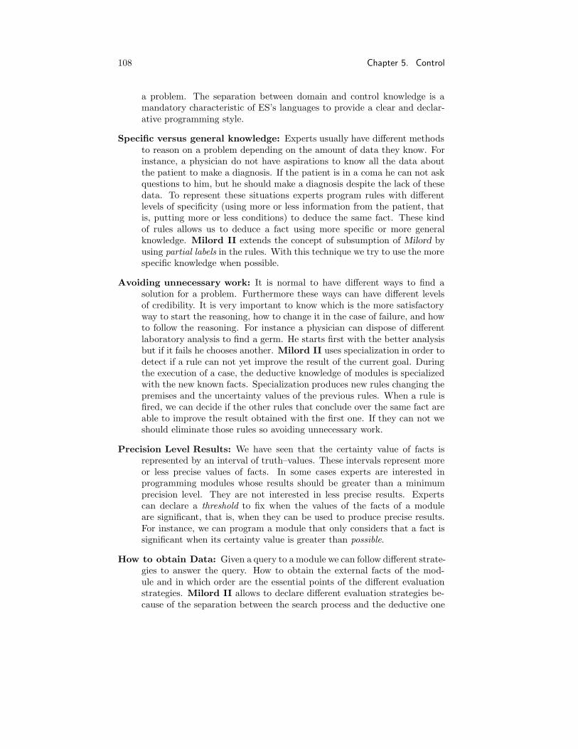
108 Chapter 5. Control
a problem. The separation between domain and control knowledge is amandatory characteristic of ES’s languages to provide a clear and declar-ative programming style.
Specific versus general knowledge: Experts usually have different methodsto reason on a problem depending on the amount of data they know. Forinstance, a physician do not have aspirations to know all the data aboutthe patient to make a diagnosis. If the patient is in a coma he can not askquestions to him, but he should make a diagnosis despite the lack of thesedata. To represent these situations experts program rules with differentlevels of specificity (using more or less information from the patient, thatis, putting more or less conditions) to deduce the same fact. These kindof rules allows us to deduce a fact using more specific or more generalknowledge. Milord II extends the concept of subsumption of Milord byusing partial labels in the rules. With this technique we try to use the morespecific knowledge when possible.
Avoiding unnecessary work: It is normal to have different ways to find asolution for a problem. Furthermore these ways can have different levelsof credibility. It is very important to know which is the more satisfactoryway to start the reasoning, how to change it in the case of failure, and howto follow the reasoning. For instance a physician can dispose of differentlaboratory analysis to find a germ. He starts first with the better analysisbut if it fails he chooses another. Milord II uses specialization in order todetect if a rule can not yet improve the result of the current goal. Duringthe execution of a case, the deductive knowledge of modules is specializedwith the new known facts. Specialization produces new rules changing thepremises and the uncertainty values of the previous rules. When a rule isfired, we can decide if the other rules that conclude over the same fact areable to improve the result obtained with the first one. If they can not weshould eliminate those rules so avoiding unnecessary work.
Precision Level Results: We have seen that the certainty value of facts isrepresented by an interval of truth–values. These intervals represent moreor less precise values of facts. In some cases experts are interested inprogramming modules whose results should be greater than a minimumprecision level. They are not interested in less precise results. Expertscan declare a threshold to fix when the values of the facts of a moduleare significant, that is, when they can be used to produce precise results.For instance, we can program a module that only considers that a fact issignificant when its certainty value is greater than possible.
How to obtain Data: Given a query to a module we can follow different strate-gies to answer the query. How to obtain the external facts of the mod-ule and in which order are the essential points of the different evaluationstrategies. Milord II allows to declare different evaluation strategies be-cause of the separation between the search process and the deductive one

5.1. Implicit Control 109
(specialization).
Programming Control: Milord II provides Horn–like metarules that can beprogrammed by experts. It is a powerful method of local control that cansimplify the deduction by eliminating rules, deducing facts and changingthe hierarchy of modules.
We divide this Chapter between the implicit control, that is, the prepro-grammed characteristics of the execution; and the explicit control as the param-eters of control that the expert can declare.
Implicit components of control are build–in in the interpreter and then theycan not be programmed. Implicit control is composed of two mechanisms, theunnecessary rules detection and the subsumption treatment. They act when wehave more than one rule that conclude over the same fact.
Control knowledge
Evaluation Type: ...
Truth Threshold: ...
Deductive Control: ...
Structural Control: ...
end control
Figure 5.1: Control declaration
Explicit components of control, that is, those that can be programmed byexperts are explained after implicit ones. These components of control knowl-edge are the threshold, the evaluation strategy and the reification and reflectionmechanism related to metarules. Figure 5.1 shows the syntactical declaration ofthe explicit control in a module.
5.1 Implicit Control
Subsumption control and unnecessary rules control are important characteristicsof the execution of a module that can not be programmed by the expert.
5.1.1 Subsumption
We have repeated along this thesis that the kind of knowledge managed by ESsis imperfect, that is, incomplete, imprecise and uncertain. Incompleteness is anusual characteristic of the knowledge managed by human experts. They havean special ability to manage and obtain useful conclusions from situations withmore or less complete knowledge. For instance, a physician needs to know dataof the patient to decide an adequate treatment. Nevertheless if the patient isin a coma then the physician should find a treatment using less data. An ES

110 Chapter 5. Control
should be capable to modelize this kind of behavior allowing to program differentsolutions to a problem with different levels of incompleteness. When possiblethe ES should work with the less incomplete (more specific or more specialized)knowledge as an expert does. That is the criteria used in Milord II.
Experts express the deductive knowledge of a module by mean of rules. Fre-quently they write several rules containing the same fact in its conclusions. Theserules can represent disjunctive paths in the proof tree of that fact, but in othercases they can represent the same path with different incompleteness level2. Wewill show two simple examples to clarify this concept. Consider the first examplefrom Terap–IA:
R051 If cotri then conclude cotri DB is slightly possibleR052 If cotri and seriousness then conclude no(cotri DB) is defi-nite
These two rules conclude over the same fact cotriDB. It is easy to see thatrule R052 is more specific than rule R051. Whenever we can apply the morespecific rule, we could also apply the more general one. We say that there is asubsumption relation between these rules. This is an example of lack of data.In this example the expert has a default rule for the case where they have nosufficient evidence3 of the seriousness of the illness. Then the fact cotri DB canbe deduced with less data.
If we consider that the fact cotri is true and the fact seriousness is unknownthe value for cotriDB would be [slightly possible, 1] using the more general rule.If we know that the fact seriousness is true we will use the more specific rule,and the result for the fact cotriDB would be [0, 0]4 or false. Notice that it is notnecessary that the truth–value of the more specific rule to be greater than thegeneral one. The second example is:
R001 If age > 60 then conclude old is possibleR002 If age > 70 then conclude old is very possible
Intuitively it is clear that the rule R002 is more specific that the rule R001.It is more specific to know that the age is greater that seventy than the age isgreater that sixty.
In Milord II as in Milord we first apply the most specific rules. If the mostspecific rule can not be applied, then the most general one is fired.
In this sense we can say that in some cases the more specific rule can not beapplied but only the more general can (default reasoning). In the cases wherethe more specific rule can be applied, the more general could be applied also.
2In Chapter 4 we had only considered that the rules with the same fact in the conclusionwere disjunctive paths.
3We say sufficient evidence in the sense that the rule would conclude a value different thanunknown ([0,1]). We will insist in this aspect in the next Section where we will talk on thethreshold control component.
4Notice that without the subsumption criteria these two rules would produce an inconsistentresult when both would be applied ([slightly possible, 1] ∩ [0, 0] = ∅).

5.1. Implicit Control 111
Our criterion is that we always apply the more specific rule if possible and inthat case the more general rule will not apply.
Remember the first example. If we know the fact seriousness then we onlyuse the rule R052. In the other case we will use rule R051.
Now we analyze the above subsumption criterion from a general point of viewin the concrete syntax of Milord II rules.
General Subsumption
Here we explain the general subsumption criterion. We think that it is inter-esting to use always the more specific knowledge in the deductive process, butwe will finally define a criterion that is a compromise among complexity andunderstandability.
First of all we analyze the subsumption criterion between two isolated rules.
Definition 5.1 (Subsumption) Given two rules R1 and R2 with premises Aand B respectively, and that they conclude over the same fact, we say that ruleR1 is more specific than rule R2 or that rule R2 is more general than rule R1,when
(A → B, 1)
Now we can simplify this criterion taking into account the different types ofpremises of Milord II.
First of all we can simplify the criterion using a property of the implication(I1, Section 3.1) used in Milord II.
(A → B, 1) ⇒ ρ(A → B) = 1 ⇒ IT (ρ(A), ρ(B)) = 1 ⇔ ρ(A) ≤ ρ(B)
Premises of rules are composed of a conjunction of predicates over facts.Facts can be of four types: boolean, logic, numeric and enumerated. We canonly compare facts of the same type. We extend the subsumption criteriontaking into account the different components of the premises of the rules.
It is easy to see from properties T5 and T1 of T functions that the followingholds:
If a ≤ b and c ≤ d then T (a, c) ≤ T (b, d)
Proof:
a ≤ b ⇒ T (a, x) ≤ T (b, x),∀xc ≤ d ⇒ T (c, y) ≤ T (d, y),∀y
⇒ T (a, c) ≤ T (b, d)
We can consider that premises of rules are composed of a conjunction ofsets of predicates over facts grouped by their type. B, L, N , and E are sets ofpredicates of types boolean, logic, numeric and enumerated respectively. Thenit is easy to extend the last property to the new one:
ρ(B1) ≤ ρ(B2)ρ(L1) ≤ ρ(L2)ρ(N1) ≤ ρ(N2)ρ(E1) ≤ ρ(E2)
⇒ ρ(B1 ∧ L1 ∧ N1 ∧ E1) ≤ ρ(B2 ∧ L2 ∧ N2 ∧ E2)

112 Chapter 5. Control
This allows us to group the conditions on sets of the same type and to applythe subsumption criterion to each group separately. Now we should test if thefollowing set of conditions hold:
(B1 → B2, 1), (L1 → L2, 1), (N1 → N2, 1), (E1 → E2, 1)
Boolean and Logic premises
Suppose the following rules:
BL1: (a1 ∧ a2 ∧ · · · ∧ an → c, α)BL2: (b1 ∧ b2 ∧ · · · ∧ bm → c, β)
If we want to test if the rule BL1 subsume the rule BL2 then:
ρ(b1 ∧ b2 ∧ · · · ∧ bm) ≤ ρ(a1 ∧ a2 ∧ · · · ∧ an)
If m ≥ n and we can found n facts such that ai = bj then it is easy to seethat ρ(a1 ∧ · · · ∧ an) = ρ(b1 ∧ · · · ∧ bn). And by the property T5 of T functionsthe following expression always hold.
T (ρ(a1 ∧ a2 ∧ · · · ∧ an), ρ(an+1 ∧ · · · ∧ am)) ≤ ρ(b1 ∧ b2 ∧ · · · ∧ bn)
In this case it is easy to see that the subsumption criterion is that rule R1 ismore general than rule R2 when A ⊆ B, where A and B are the set of booleanand logic conditions of rules BL1 and BL2 respectively.
Numeric and enumerated premises
This case is not so easy as the logic and boolean premises. Numeric expressionscan be a set of arithmetic expressions among facts and numbers. Each conditioncan contain several facts, and two conditions can predicate over the same fact.Consider the following example:
(a − b > 3 ∧ b < 6 → c, α)(a < 12 → c, β)
In this case it is easy to see that the second rule subsumes the first one,because:
ρ(a − b > 3 ∧ b < 6) = ρ(a > b + 3 ∧ b < 6) = ρ(a < 9 ∧ b < 6) =T (ρ(a < 9), ρ(b < 6)) ≤ ρ(a < 9) ≤ ρ(a < 12)
In general the problem can be reduced to two inequation systems, each onecomposed by the conditions of each rule. After finding the solutions of the twosystems, we can compare each variable of the systems, and show if one systemimplies the other. In the last example:
a − b > 3b < 6
⇒a < 9b < 6
⇒ a < 12

5.1. Implicit Control 113
Finding solutions for an inequation system is a complex task. It is easy tosee that in the case of enumerated premises the problem is similar, but muchmore complicated (remember the operations on fuzzy sets explained in the Sec-tion 3.2.3).
In real programs experts normally do not write very complicated conditions.Furthermore a complex subsumption criterion is an impediment more than a helpto the understandability of subsumption when the expert writes his program.
For all these reasons in the case of numeric and enumerated premises weconsider that there is a subsumption relation between two rules when the factscontained in the premise of one rule are contained in the set of facts of thepremise of another rule as in the logic and boolean case.
Subsumption in depth: Partial Labels
There are added problems that have not been addressed yet. Till now we haveonly worked with two isolated rules. The last criterion is not enough for catchingall the subsumption relations when we have many rules. For instance considerthe following set of rules:
R1 : a ∧ b ∧ c ∧ d → gR2 : e ∧ f → gR3 : c → eR4 : a ∧ b → f
It is easy to see that there is a hidden subsumption relation between the rulesR1 and R2. Considering the usual chaining of rules we can obtain that the setof facts necessary to fire the rule R1 is a, b, c, d, and for the rule R2 is a, b, c.R1 is more specific than R2. In this case we do not only compare the premisesof the rules but the set of facts in the deduction tree below the fact along twodifferent paths.
We should not forget that we are thinking on an isolated module. If weconsider all the modular structure then we can find new hidden subsumptionrelations. Suppose that the rules in the last example are distributed in twodifferent modules.
M1 :
RM1
1 : M2/f ∧ M2/c ∧ d → g
RM1
2 : M2/e ∧ M2/f → gM2 :
RM2
1 : c → e
RM2
2 : a ∧ b → f
We can find the same subsumption relation than in the first example.In our system we only find local subsumption relations. Other subsumption
relations are ignored.Now we describe a partial solution to this type of hidden subsumption rela-
tions using partial labels.The first idea is to find the set of facts in the deduction tree below the facts.
We would compare them in order to find the subsumption relations. Apart ofthe complexity of this task, there is another problem. We consider subsumptionwith respect to the data that has been really used to deduce a fact. We do not

114 Chapter 5. Control
know a priori the data that will be necessary to do this. We can not predictwhich of the conjunctive paths will be successful. Then we can not build labelsstatically but at runtime.
Now we explain the method used in Milord II. This is based on partiallabels. Specialization allows us an easy implementation of this kind of task.
We will illustrate the explanation with the example in the Figure 5.2. Thecomplete label of a fact in a rule is composed of terminal nodes of the proof treeconsidering an isolated module. Terminal nodes of a module are the importedfacts and the prefixed facts (those facts belonging to the submodules).
R1〈a, b, c, d〉 : a ∧ b ∧ c ∧ d → gR2〈〉 : e ∧ f → gR3〈c〉 : c → eR4〈a, b〉 : a ∧ b → f
a;
R1〈a, b, c, d〉 : b ∧ c ∧ d → gR2〈〉 : e ∧ f → gR3〈c〉 : c → eR4〈a, b〉 : b → f
b;
R1〈a, b, c, d〉 : c ∧ d → gR2〈a, b〉 : e → gR3〈c〉 : c → e
c;
R1〈a, b, c, d〉 : d → gR2〈a, b, c〉 : ∅ → g
Figure 5.2: Example of subsumption.
Initially we can build the partial labels of each rule identifying the facts inthe premise of the rule that are terminal nodes. In our example all the conditionsin the rule R1 are terminal nodes. Conditions of the rule R2 are not terminalnodes, they are deducible nodes (by the rules R3 and R4).
When a rule is specialized with a fact that has been deduced by another rule,the first rule extends its label with the label attached to the other rule. In theexample when rule R4 is fired and the fact f specializes the rule R2, the newpartial label of R2 is the union of the old label (empty) and of the label of thefired rule (〈a, b〉).
Before firing a rule we can compare its label with the labels of the other rulesthat conclude over the same fact. In the case a subsumption relation betweentwo rules is detected, we act as explained before. In the last specialization stepof the example, we can observe that the rule R2 can be fired but its label isincluded in the label of the rule R1. In that case the rule R2 is more specificthan the rule R1 and it is not fired until we know if rule R1 is able to be fired.
Finally we can summarize the design decisions adopted for the practicalimplementation of subsumption relations.
• We consider only local subsumption relations inside modules. The rela-tions that can be detected building the partial labels of the rules duringexecution time.
• Runtime labeling of rules allow us to detect cases of hidden subsumptionrelations.

5.1. Implicit Control 115
• We consider that the specificity of a rule with respect to the other rulesconcluding the same fact is determined by the inclusion relationship oftheir partial labels. A rule is more general than another if its partial labelsare included into those of the other rule.
• We only use the more specific rules if possible; otherwise we use the moregeneral ones.
5.1.2 Unnecessary Rules
In the Section above we have seen that the evaluation of a fact can be carriedout by one or more rules. All these rules can contribute to the evaluation of afact taking into account that in the case of rules with a subsumption relationonly a rule will be used. Now we only consider the set of rules that effectivelycan take part in the evaluation of a fact.
These rules will be specialized using a concrete search strategy by means ofthe Specialization inference rule. We can compose the results of these rules bymeans of the Composition inference rule, as seen in Section 4.2.3. It is easyto see that the intersection of intervals of truth–values leads to more precise orequal values. Each rule can contribute then to give more precision to the finalresult.
Suppose the situation where we have obtained a provisional value to a fact(a rule has been totally specialized). We can now consider if the remaining rulesconcluding the same fact can give more precision to the fact.
The maximum precision given to the conclusion of a rule is limited by the cer-tainty value of the rule. Consider a rule with premise value [a i, aj ] and certaintyvalue [aρ, 1]. The conclusion of the rule is given by
MP ∗T ([ai, aj], [aρ, 1]) = [T (ai, aρ), 1)] = [ar, 1] ,where ar ≤ aρ
Then it is easy to see that the value of the conclusion of the rule will be moreimprecise or equal that the precision of the value of the rule. There are nodifferences in the case of negative conclusion because the negation does notchange the precision. When the system obtains a new provisional value for afact, we test if the rules associated to the fact are necessary or unnecessary.
If the provisional value is [ρpp, ρ
op] and the value of the rule is [ρr, 1], if the
conclusion of that rule is affirmative then the rule will be unnecessary if andonly if ρr ≤ ρp
p. If the conclusion is negative then the rule will be unnecessary ifand only if ρr ≥ Nn(ρo
p).We apply this test again when a rule is specialized, because specialization
deals with more imprecise or equal truth–values of rules. This method allowsus to save unnecessary deduction and avoids to demand information outside themodule without necessity.
Specialization of rules results in new rules with new truth–values. Thenwe can apply this method when a rule is specialized. Notice that it is an im-provement with respect to other system that do not use specialization (includingMilord). They could only compare the rules before or after firing them. In the

116 Chapter 5. Control
last case all the questions related to a rule would be made. This can be avoidedthanks to the previously explained test.
5.2 Threshold
Remember that the goal of the inference engine of Milord II is to obtain valueswith the maximum precision. Despite this we can obtain final values of factswith so little precision that an expert can consider not to be significant, thatis, like unknown. Milord II introduces a parameter that controls the minimumprecision of facts in order to consider that they are significant. This parameteris local to each module, then we can control the precision level needed to solvea concrete problem.
This mechanism of control is named the threshold (Th) of a module. It isa linguistic label belonging to An and represents the minimum value a deducedfact must have to be significant. The default threshold value of Milord II isthe second term A2 of the chain An of truth–values. MYCIN (Shortliffe, 1976)had certainty factors lying in the interval [0, 1]. The threshold used was of 0.2.An example of threshold declaration is:
Truth Threshold: possible
Now consider the following general rule:
(a1 ∧ a2 ∧ · · · ∧ am → b, [ρr, 1])
We can calculate the final value of the conclusion5 b:
ρ(b) = MP ∗T (ρ(a1 ∧ a2 ∧ · · · ∧ am), [ρr, 1])
ρ(a1 ∧ a2 ∧ · · · ∧ am) = T ∗(ρ(a1), ρ(a2), . . . , ρ(am))
Considering that ρ(ai) = [ρpai
, ρoai
], then:
T ∗(ρ(a1), ρ(a2), . . . , ρ(am)) = [T (ρpa1
, ρpa2
, . . . , ρpam
), T (ρoa1
, ρoa2
, . . . , ρoam
)]
ρ(b) = MP ∗T ([T (ρp
a1, ρp
a2, . . . , ρp
am), T (ρo
a1, ρo
a2, . . . , ρo
am)], [ρr, 1]) =
ρ(b) = [T (T (ρpa1
, ρpa2
, . . . , ρpam
), ρr), 1] = [T (ρpa1
, ρpa2
, . . . , ρpam
, ρr), 1]
And finally:
T (ρpa1
, ρpa2
, . . . , ρpam
, ρr) ≤ Min(ρpa1
, ρpa2
, . . . , ρpam
, ρr)
Notice that the precision of the conclusion of a rule depends on the minimumtruth–values of the rule and its conditions. Given a rule with minimum truth–value less than the threshold, it concludes the interval [0, 1]. The same happenswhen it exists one condition of the rule whose value is less than the threshold.
5Because we are talking on precision we will use only positive rules. Negative rules producethe same results on precision.

5.3. Evaluation Strategy 117
5.3 Evaluation Strategy
At this moment we know many aspects of Milord II. We have talked about themodular structure, the uncertainty, and the deductive component. We know howa knowledge base is specialized using the above implicit control. To specializethe deductive knowledge of a module it needs to know external data (from theuser and from its submodules). But until now we have not explained how thisinformation is obtained. In the Figure 4.2 we can see that the search processasks questions to the user and then passes information to the deductive processin order to specialize the knowledge base. In this Section we explain how thesearch process obtains information from the user and from its submodules.
The search process is goal directed inside each module. Given a goal, that is,a fact to be evaluated in a module, the evaluation goes by asking the necessaryquestions to the user and to its submodules in order to evaluate the goal withthe maximum precision.
In Milord II there are three evaluation strategies, named lazy, eager andreified strategies. These strategies are declared locally to each module. Lazyand eager evaluation types are radical strategies in the sense that they use theminimum information in the case of lazy, or the maximum information in thecase of eager. Other strategies could be defined thanks to the separation betweensearch and deductive processes as explained in Section 4.1.1. Before explainingin detail these strategies we give a brief summary:
Lazy: A module with this evaluation strategy asks questions to the user andto its submodules only in the case where this questions are necessary toreach the current goal. This strategy is used by default.
Eager: Given a goal to an eager module the following actions are done: it asksto the user all the imported facts of the module; and it asks also all theexported facts of its submodules.
Reified: This kind of evaluation strategy do not differs of the eager one in theform of asking questions. We will explain in detail this kind of evalua-tion when explaining the reification and reflexion mechanisms in the nextSection.
5.3.1 Lazy
A module with lazy search strategy finds the cheapest path to obtain a solutionfor a goal. This is a dynamic task in the sense that the module finds the nextfact to be asked looking at the current state of that module (values of the factsand current rules). This determines a search cycle consisting in finding thenext question that is relevant to the goal (user or submodules) and updatingthe module (by means of the specialization of the knowledge base). This cycleconsisting on finding a question and specializing a module is repeated until thegoal is reached.

118 Chapter 5. Control
We should remember which are the components of a module that participatein the evaluation of a fact. A fact of a module can be evaluated by the user(import), by its submodules, by means of needs true or needs false relations (seeSection 4.4.1), by a function associated to a fact (see Section 4.4.1), or by therules of the deductive knowledge of the module.
Given a goal to a module the algorithm sketched below shows how the modulefinds the questions that are needed to reach the current goal of the module. Thatprocess only returns which is the next fact that is necessary to obtain. This is arecursive algorithm because the initial goal to the module produces new internalsubgoals that in its turn use the same algorithm.
1. Goal of a submodule. If the goal is a path to a submodule of the currentmodule, and if that submodule is visible, then the algorithm returns thatpath (it will be asked to the submodule).
2. Goal belonging to the import interface. In this case we must considerif that goal has needs6 relations with other facts. If the goal has notneeds relations the algorithm returns the same goal (it will be asked to theuser); otherwise the needs relations must be satisfied and then we applyrecursively the function to the first fact of a non solved need relation.
3. Goal with a function attribute. Now the evaluation of the goal depends onthe evaluation of the function attribute. In this case we apply recursivelythis algorithm to the first fact with no value that belongs to the function.We iterate this process until all the facts of the function are obtained.Finally the function is evaluated and its result attached to the fact.
4. Goal that can be deduced by means of rules. In this case we start a depthsearch on the rules of the deductive knowledge of the module. This will beexplained in the rule search Section.
Notice that the algorithm finally returns a path to a submodule of the currentmodule, or a fact belonging to its import interface.
Rule Search
Before starting the rule search we order the set of rules that are able to deducea fact with the following criteria.
1. Rules more specific first. We try to find solutions first using the morespecific rules.
2. With rules with no subsumption relations we try first the more preciserules. A rule is more precise than another when its truth–value is moreprecise than that of the other rule. Notice that this order can changeduring the execution because of the specialization of rules. We try firstthe solutions expected more precise.
6Need relations are those explained in Section 4.4.1, that is, Needs, Needs true andNeeds false.

5.4. Reification and Reflection Mechanisms 119
3. Finally we maintain the order of rules given by the expert.
When we select a rule we maintain the writing order of the conditions of thatrule (left to right). With these considerations the search strategy is depth first7.We apply recursively the above procedure until a fact is found.
5.3.2 Eager
The eager strategy is radically different from the above one. Now we have noteconomical criteria to find the questions. Given a goal to a module, that moduleasks all the facts of its import interface, and all the facts belonging to the exportinterfaces of its submodules.
The ordering of these goals is that of the declarations given by the expert,that is, first the facts of the import interface of the module with its originalorder, then the facts of the export interface of its submodules with the order ofdeclaration in the submodules. In this kind of search only the needs relationsare taken into account when asking questions to the user.
5.4 Reification and Reflection Mechanisms
Above we described the implicit and static mechanisms of control that are usedin Milord II. Implicit mechanisms affect the specialization process made in thedeductive knowledge of modules. We only use the rules that can improve theresults (those with more precision) and those with more specific knowledge whenpossible. These implicit mechanisms of control can not be programmed by theexpert.
The expert can declare which is the precision level of the modules and thekind of evaluation used into them. The search process is effected by the implicitmechanisms cited above and it determines which questions and in which orderthey will be asked to the user and to the submodules. Now we are interested inthe dynamic aspects of control, that is, the control programmed by the expertby means of metarules.
We have presented a complete description of the execution of modules. Givena query to a module and depending of the kind of search strategy, the modulestarts making questions to the user, to other modules and making deductionsby means of the specialization of modules. Now we complete the internal com-ponents of a module adding the meta control component into its structure. Asintroduction we explain the components shown in the Figure 5.3).
Object Level: The object level of a module is composed by the facts and therules. It is an active component. Given a goal to a module, it finds that goalby inspecting the rules, relations, functions and so on, and asking questionsto the user (import interface) and to its submodules (hierarchy). It followsthe search strategy (evaluation type) of the module and specializes the
7This is not exactely true because of the need relations modify that search strategy.

120 Chapter 5. Control
Communication
-
MODULE
Reflection Reification
?
6
Object Level
Meta Level
Figure 5.3: Control cycle.

5.4. Reification and Reflection Mechanisms 121
rules following the implicit control (subsumption and unnecessary rules)and the specialization process with the new external information obtained.The reification process informs the meta level about the actions performedby the object level. The actions give values to facts and specialize rules.
Meta Level: The meta level of a module is composed of a set of metarules(classified in deductive rules and structural rules). It is a passive com-ponent. It is continuously looking at the behavior of the object level. Itmakes actions when the conditions of a metarule hold. The reificationprocess informs then the meta level about the actions done by the objectlevel, and the meta level acts on the object level by reflecting actions.These actions affects the deductive knowledge (deductive control) and thehierarchy (structural control) of the module. The actions proposed by themeta level are mandatory to the object level.
For instance, if the object level informs the meta level that the patient is aman, then the meta level reflects an action consisting in eliminating the specificrules for women.
Before describing the syntax of metarules we should see which are the com-ponents of the object level that are reified to the meta level. Static reificationinforms the meta level about static components of the deductive knowledge, asrelations, submodules, etc. Dynamic reifications informs the meta level aboutthe specialization process, as new deductions, specialized rules and so on.
5.4.1 Static Reification
The static reification informs the meta level of several characteristics of themodule that do not change during the execution, as the relations among facts,the type of facts, the submodules, the threshold, the set of linguistic terms andthe kind of search strategy.
Relations: It is the meta predicate name of relation (the predefined relationscan also be used) with two arguments corresponding to the facts related(the facts can be valid paths from the module). The relation is from fact1to fact2.
name of relation(fact1, fact2)
Types: The predicate that says that a fact belongs to a concrete type:
type(fact, type of fact)
where type of fact ∈ boolean, logic, numeric, class, list of symbols,name. An enumerated fact is named with the set of symbols of the typeof that fact (list of symbols) or its name (name) (see Section 4.4.1).
The static reification is performed before the execution of the module becauseit does not change during the execution.

122 Chapter 5. Control
5.4.2 Dynamic Reification
The current object level theory (OLT) is the set of rules of a module. Thecurrent meta level theory (MLT) is the set of meta–rules of a module, plus theinstances of the user defined metapredicates, that were the defined in the Sectionabove. Dynamic reification is composed of the predicates K, WK and P thatare related to the value of facts, and the active submodules of the module.
First of all the minimal literal definition is given. It is composed of the setof facts deduced in the OLT with the most precise value.
Definition 5.2 (Minimal Literal) We define the minimal literal OLT as
OLT ∗ = (p,W )|p is a literal, and W =
n⋂
i=1
Vi such that (p, Vi) ∈ OLT
Meta–predicate K
K(p, V ) means that V is the minimal interval such that the proposition (p, V )belongs to the OLT. There is a close world assumption on this predicate. Thereflection rules are:
(p, V ) ∈ OLT ∗
`M K(p, V )
(p, V ) 6∈ OLT ∗
`M ¬K(p, V )
The reflection process maps the meta level theories into object level literals.The reflection rule that relates MLT with OLT is defined as:
`M K(p, V )
`O (p, V )
Meta–predicate WK
WK(p, V ) means that (p, V ) is deducible in the OLT, i.e. OLT `O (p, V ).¬WK(p, V ) means that OLT `O (p, V ′) with V ′ 6= [0, 1] but V ′ 6⊆ V .
(p, V ) ∈ OLT ∗ and V ⊆ V ∗
`M WK(p, V ∗)
(p, V ) ∈ OLT ∗ and V 6⊆ V ∗
`M ¬WK(p, V ∗)

5.4. Reification and Reflection Mechanisms 123
Meta–predicate P
P (p) means that (p, V ) belongs to the deductive closure of OLT being V 6= [0, 1].If at the moment of the upwards reflection the computing of the deductive closurefor p is not finished neither P (p) nor ¬P (p) will be generated.
OLT `O (p, V ) and V 6= [0, 1]
`M P (p)
OLT 6`O (p, V ) and V 6= [0, 1]
`M ¬P (p)
Examples of these predicates can be:
K(fever,[very possible,1]WK(pneumonia,[possible,1]P(cotri)
The first example means that the fact fever has been deduced in the OLTtheory with value [very possible, 1] and that value is the most precise one. Thesecond example says that the fact pneumonia is provisionally deduced with value[possible, 1], but it could be deduced with more precision. The last examplemeans that the fact cotri is proved in the OLT theory with a value differentfrom unknown.
After defining which is the knowledge that the meta level contains in a con-crete moment of the execution of a module, we explain the syntax of the meta-rules of Milord II. We distinguish between deductive and structural metarules.The first ones are related to the deductive knowledge of the module that containsthem, and the other to the submodule structure of that module.
premisse-meta ::= condition-meta and premisse-meta |condition-meta
condition-meta ::= mconditio |no(mconditio )|
mconditio ::= metapredid (conditionterm , ..., conditionterm )
conditionterm ::= operation (conditionterm ,..., conditionterm )|
metafunctid (conditionterm , ..., conditionterm )|
conditio
Figure 5.4: Syntax of the premises of metarules.
See the Figure 5.4 for the complete syntactical description of the premises ofmetarules. Where metapredid are the above metapredicates (K, WK and P) plusarithmetic predicates (le, ge, gt and lt), set operators (member, diff and atom).At the moment we only use plus as operations. Finally the metafunctions arerelative to array functions (for instance transpose).

124 Chapter 5. Control
5.4.3 Deductive Control
The deductive control (see the Figure 5.5) affect the deductive knowledge of amodule by inhibiting rules or deducing the above metapredicates. In some casesit is interesting to simplify the set of rules to avoid unnecessary deductions, orto deduce facts despite of the object level.
mrr ::= metaid If premisse-meta Then filters-mrrfilters-mrr ::= filter-mrr filters-mrr | filter-mrrfilter-mrr ::= inhibit rules relation-id pathpredid |
inhibit rules pathpredid |prune pathpredid |conclusion-meta
conclusion-meta ::= mconclusion |no (mconclusion )
mconclusion ::= metapredid (conclusionterm , ..., conclusionterm )
conclusionterm ::= operation (conclusionterm , ..., conclusionterm )|
metafunctid (conclusionterm ,..., conclusionterm )|
formform ::= predid | $symbol
(form op form)
Figure 5.5: Syntax of the deductive control.
Inhibit Rules: This action inhibits all the rules containing the fact pathpre-did into their premises. We can introduce optionally a name of relationrelation-id and then the rules inhibited will be those containing in itspremises a fact related with pathpredid.
Prune: It inhibit all the rules belonging to the deductive tree of the fact path-predid.
Conclude: Metarules can give a value to a fact of the object level. Meta levelhas the maximum priority and then the value of a fact given by the metalevel will be definitive. This implies to inhibit the rules deducing this fact.
5.4.4 Structural Control
The metarules of the structural control (see the Figure 5.6) are designed tomodify the hierarchy of a module by inhibiting modules or declaring new ones(dynamic modules); they can also stop definitely the execution (for instance,when the system is out of domain).
Filter: A metarule can inhibit (filter) submodules of a module. That meansthat all the facts exported by the filtered submodule will be unknown.

5.4. Reification and Reflection Mechanisms 125
mre ::= metaid If premisse-meta Then filter-mrefilter-mre ::= filter amodidlist |
order amodidlist |Open (conclusionterm , ..., conclusionterm )|
Module (conclusionterm , ..., conclusionterm )|
Inherit (conclusionterm , ..., conclusionterm )
amodidlist ::= amodid amodidlist | amodidmrx ::= metaid If premisse-meta Then exceptionexception ::= definitive solution predid |
stop
Figure 5.6: Syntax of the structural control.
Order: When we use eager evaluation in a module, the order of questioning thesubmodules is by the writing order given by the expert. Sometimes it isinteresting to change this order at run time. This actions allow to changethis order when a set of conditions hold.
Open, Module and Inherit These declarations are equivalent to the corre-sponding normal submodule declarations, but they are performed dynami-cally. The following example (from Spong–IA) shows the dynamic creationof a submodule by means of the dynamic instantiation of a generic mod-ule. Given a value for the enumerated fact DM/taxon, z, with certaintyvalue [min,max]. If min is greater than the threshold of the moduleDM , cut, and z is a submodule of DM , then a submodule is created,with local name z. That module is the instantion of the generic moduleRefinement method with the modules DM/z and T .
M0001 if K(((DM/taxon ,$z), int($min,$max)) andthreshold(DM, $cut) and gt($min,$cut) andsubmodule(DM, $z) thenModule(=($z,Refinement method(DM/$z, T)))
Definitive Solution and Stop: These are exceptional actions. In some casesthe expert wants to stop the execution given the value of a fact (definitivesolution) or nothing (stop). This is useful when the ES is out of domain.
Apart from the kind of process used to ask questions in the different evalua-tion types, we must make distinctions between them with respect to the reifica-tion and reflexion mechanisms and the specialization.
Lazy: Given a query to a lazy module,
1. It starts finding a question to the user or to a submodule useful toreach the current goal (see Section 5.3.1).

126 Chapter 5. Control
2. It obtains the value for this question and reifies the result (value ofthe fact) to the meta level.
3. The meta level tries to fire metarules. Now there is a looping betweenthe meta level and the object level. It consists in reflecting a resultto the object level (specialize, inhibit rules, filter submodules, and soon), to execute the action at the object level, and reify its results. Itis an iterative process until the meta level reflects nothing.
4. Finally the object level specializes its knowledge with the answer tothe first question. And it returns to the first step.
This process continues until a value for the initial query is found.
Eager: Given a query to an eager module,
1. It does the same actions that points 1 to 3 of the lazy strategy. Thedifference is that an eager module ask all the questions of its importinterface and of all the export interface of its submodules.
2. Finally the module specializes with all the questions made followingthe same dialog with the meta level as before.
Reified: Given a query to a reified module,
1. The first step is similar of that of the eager strategy, but the rules ofthe module are also reified. In this case specialization is not used andall the deduction is made at meta level.
2. Finally the module gets the results reflected by the meta level.
Usually applications use the lazy and eager evaluations as a form of obtainingthe information from the user. An example of module evaluation type reified isgiven in Section 6.6.
5.5 Conclusions
In this Chapter we have completed the description of Milord II by presentingthe control. We have explained the part of the control that is implicit in Mi-lord II and the one that can be programmed by the user.

Chapter 6
Applications
In the introduction of this thesis we put emphasis on the applicability of Mi-lord II to build real world systems. After the syntactical and semantical de-scription of all the components of the language and the system, this last Chapterdeals with the systems that have been developed and that are currently runningwith Milord II.
Thanks to these application and to the enthusiastic collaboration of the ex-perts we have been able to bring Milord II to the actual state. In the introduc-tion we have distinguished Milord II from other systems by its purpose. Themain purpose of Milord II are the application development. The languagesdirected to the applications are designed following a bottom–up methodology.The development of the applications and of Milord II have been in a mutualfeedback cycle.
Despite the great number of problems raised by the paralell developmentof real applications and of Milord II, it has brougth a fruitful collaboration.From the developer point of view, real applications are an interesting source ofnew problems. Experts have taken advantage of the bottom–up development bybeing allowed to introduce these suggestions to the system design.
6.1 Introduction
We introduce the main applications developed with Milord II. They are dif-ferent applications and each one has contributed with their own problems andsolutions to Milord II development.
In the first part of this Chapter we explain three ES application (Terap–
IA, Spong–IA, and Ens–AI). Terap–IA is presented more extensively than theothers. Finally we explain two examples. The firs one deals with fuzzy controland the other with the propagation of belief in bayesian polytrees.
127

128 Chapter 6. Applications
6.2 Terap-IA
Terap-IA is a medical application for pneumonia treatment developed at the IIIA
by Dr. Pilar Barrufet using Milord II. It is a collaboration with the MataroHospital directed by Dr. Albert Verdaguer. A Ph.D. Thesis based on Terap–IA
will be presented soon by Dr. Pilar Barrufet. Terap–IA is the natural exten-sion of a previous expert system named Pneumon–IA for pneumonia diagnosis(Verdaguer, 1989) developed using Milord (Sierra, 1989).
6.2.1 Motivation and Goals
The most common cause of mortality related with infectious processes is thepneumonia (it is the sixth death most common cause at EEUU).
The death rate of patients affected by pneumonia that needs hospitalization,is very high. About of 54% of gravely ill patients at the intensive care unitdied, and about 20% were old people. In other cases the death rate is about5.7%. The death rate of patients that do not need hospitalization is lower thanthose considered above. Despite this, every pneumonia case needs an urgentdiagnosis and treatment. Erroneous initial diagnosis can be fatal in some cases.For instance, an initial diagnosis of pneumococic pneumonia in a patient withlegionella pneumonia can be fatal because of late adequate treatment.
The goal of Terap–IA ES is to deduce the best antibiotic treatment in thecase of a pneumonia caused by only one etiologic agent or considering differentetiologic hypothesis (definitive diagnosis are about 50%). In the last case weshould combine the set of antibiotics corresponding to each germ. Thus it musttake into account a set of criterion used in the antibiotic combination.
6.2.2 Architecture
We describe the process of obtaining the treatment of pneumonia for a patienthaving a previous diagnosis (set of possible germs). The goal is to produce anadequate treatment for the case using the previous diagnosis and the data of thepatient . The architecture of Terap–IA is graphically represented in Figure 6.1.
1. We start with the set of groups of antibiotics1 used for the pneumoniatreatment. Initially we consider that the uncertainty values of these groupsof antibiotics are all true.
2. General conditions: A set of general conditions obtained from the patientis used to filter those groups of antibiotics. Filter these groups consist inchanging its uncertainty value by means of rules (remember that initially
1The list of 27 groups of antibiotics is the following: Quinolones, Tetraciclin, TetraciclinRetard, Cotrimoxazol, Sulfamids, Vancomicine, Teicoplanine, Aminoglucocids, Metronidazol,Clindamicine, Carbapenems, Isoniacida, Rifampicina, Etambutol, Pirazinamida, Anfoteric-ina B, Aciclovir, Ganciclovir, Vidarabina, Ribaravina, Amantadine, Rimantadine, Penicilline,Macrolids, Betalactamases Inhibitory, Cefalosporines, and Monobactams.

6.2
.Tera
p-IA
129
CombinationCriterion
Groups of Antibiotics
Antibiotics
Previous Diagnosis
Antibiotics
Antibiotics
Antibiotics
Groups of Antibiotics
AntibioticsCombinations
AntibioticsCombinationResult
- Gestation- Breast-Feefing- Alergy- Renal Failure- Genetic Elements
- Spectrum- Cost- Other conditions- Seriousness
- Interactions- Contrary Effects
...
...
...
...
Figu
re6.1:
Arch
itecture
ofTera
p–IA
app
lication.

130 Chapter 6. Applications
all the groups have the value true). The order of filtering is that of thefollowing items2.
(a) Gestation
(b) Breast–feeding
(c) Allergy
(d) Renal Failure
(e) Genetic Elements
For instance the expert states that If the patient has renal failure thenthe certainty value of Aminoglucocids decreases from sure to possible. Theresult of this filtering is the same groups of antibiotics that we got initiallybut with their truth–values now adequated to the current case.
3. The starting point is a set of germs that are selected from a previousinitial diagnosis of the patient. These germs are the possible causes of thedisease3. The user selects a set of these germs.
4. For each germ selected we filter the above groups of antibiotics:
(a) Bacterian Sensibility: Given a germ and the groups of antibioticswith its certainty value for the germ, the process of filtering selectsthe groups of antibiotics that can be used in a treatment for this germ.
(b) Seriousness: For each group of antibiotics the seriousness of the pa-tient determines the concrete antibiotics of that group that are ade-cuate for the treatment.
(c) Interactions: Filter the concrete antibiotics that have interactionswith other treatments.
(d) Contrary Effects: Filter the concrete antibiotics taking into accountthe contrary effects of other treatments.
The result of this phase is a set of concrete antibiotics with a truth–valueassociated for each germ considered.
5. When the system has a set of antibiotics one for each germ consideredthen:
(a) Antibiotic Combination: It combines the treatment for each germreturning a global treatment (a combination of antibiotics).
2The filtering of the groups of antibiotics is not dependent of the germ selected.3The list of the 24 germs is the following: Mycoplasma, Coxiella Burnetii, Chlamydia
Psitacii, Chlamydia Pneumoniae, Legionella Pneumophila, Pneumococcal Pneumonia, Anaer-obis, Enterobacteria, Influenza Virus, branh, Pseudomonas, Meningococcus, S Pyog, S Au-rea, Aspergilus, Crip, Nocar, Cytomegalovirus, Varicela–zoster Virus, Herpes Simplex Virus,Eptein–Barr Virus, Respiratory Syncitial Virus, Adenovirus and Haemophilus Influenzae.
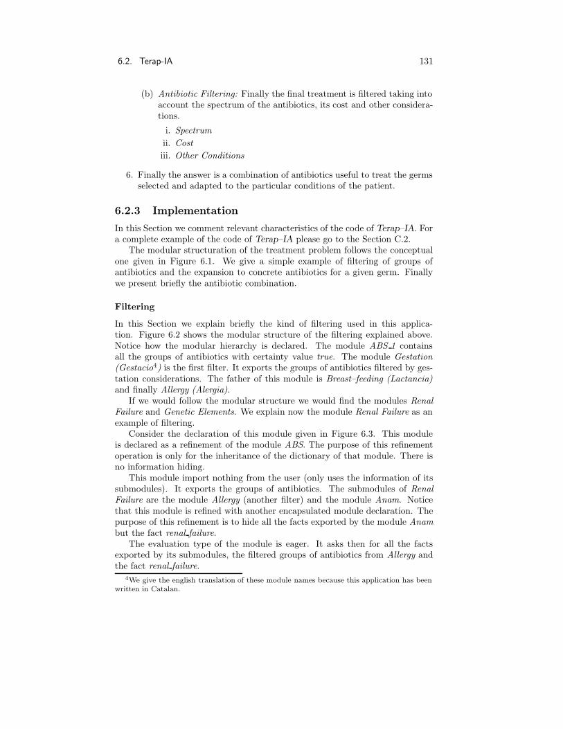
6.2. Terap-IA 131
(b) Antibiotic Filtering: Finally the final treatment is filtered taking intoaccount the spectrum of the antibiotics, its cost and other considera-tions.
i. Spectrum
ii. Cost
iii. Other Conditions
6. Finally the answer is a combination of antibiotics useful to treat the germsselected and adapted to the particular conditions of the patient.
6.2.3 Implementation
In this Section we comment relevant characteristics of the code of Terap–IA. Fora complete example of the code of Terap–IA please go to the Section C.2.
The modular structuration of the treatment problem follows the conceptualone given in Figure 6.1. We give a simple example of filtering of groups ofantibiotics and the expansion to concrete antibiotics for a given germ. Finallywe present briefly the antibiotic combination.
Filtering
In this Section we explain briefly the kind of filtering used in this applica-tion. Figure 6.2 shows the modular structure of the filtering explained above.Notice how the modular hierarchy is declared. The module ABS 1 containsall the groups of antibiotics with certainty value true. The module Gestation(Gestacio4) is the first filter. It exports the groups of antibiotics filtered by ges-tation considerations. The father of this module is Breast–feeding (Lactancia)and finally Allergy (Alergia).
If we would follow the modular structure we would find the modules RenalFailure and Genetic Elements. We explain now the module Renal Failure as anexample of filtering.
Consider the declaration of this module given in Figure 6.3. This moduleis declared as a refinement of the module ABS. The purpose of this refinementoperation is only for the inheritance of the dictionary of that module. There isno information hiding.
This module import nothing from the user (only uses the information of itssubmodules). It exports the groups of antibiotics. The submodules of RenalFailure are the module Allergy (another filter) and the module Anam. Noticethat this module is refined with another encapsulated module declaration. Thepurpose of this refinement is to hide all the facts exported by the module Anambut the fact renal failure.
The evaluation type of the module is eager. It asks then for all the factsexported by its submodules, the filtered groups of antibiotics from Allergy andthe fact renal failure.
4We give the english translation of these module names because this application has beenwritten in Catalan.

132 Chapter 6. Applications
Figure 6.2: Example of filtering.

6.2. Terap-IA 133
The rules of this module give a certainty value to a set of groups of antibiotics.Notice that the role of the only metarule of the module is to give a value to thegroups of antibiotics that has not been deduced by the module.
M001 If K(x/$y,$c) and NP($y) then conclude K($y,$c)
The meaning of this metarule is the following: given any fact of the submod-ule x (x/y) with any value c, such that y has not been deduced by the currentmodule (NP ($y))5, then we give to the fact y of the module the value c.
This facts maintains the same value that the given by the submodule x (thatcorresponds to the module Allergy). All the filtering modules follows this kindof structure.
Module renal failure:ABS =Begin
Module x = allergyModule anam R= anam:
Begin
Export renal failureEnd
Export quinol, tetras 1, tetras 2, cotri, sulfas, vanco, teico,amino, metro, clinda, carbapen, INH, RFM, ETM, PZ,anf B, ACV, GCV, ARA A, RBV, AMD, RMD, peni,macrol, b lactam inh, cef, monobac
Deductive knowledge
Rules:
R001 If anam R/renal failurethen conclude no(tetras 1) is s
R002 If anam R/renal failurel then conclude tetras 2 is pR003 If anam R/renal failure then conclude amino is pR004 If anam R/renal failure then conclude anf B is pR005 If anam R/renal failure then conclude AMD is pEnd deductive
Control knowledge
Evaluation Type: eager
Deductive Control:
M001 If K(x/$y,$c) and NP($y) then conclude K($y,$c)end control
End
Figure 6.3: Module Renal Failure.
After the filtering of the groups of antibiotics for each germ, we find theconcrete antibiotics for the treatment. In Figure 6.4 there is a simple case oftreatment for the germ Pneunomia Mycoplasma.
5The metapredicate NP means ¬P (see Section 5.4.2).

134 Chapter 6. Applications
This module inherits the facts of the dictionary from the module Antimicro-bians. It exports concrete antibiotics. The submodules of this module are theantecedent of the patient Antecedents and the last filter Renal failure. Noticethat this module is refined in order to only select the groups of antibiotics thatare useful for this germ (bacterian sensibility). The rules determine the valuesfor the concrete antibiotics exported.
Antibiotic Combinations
The initial diagnosis is a set of possible germs. The system deduces a treat-ment for each germ of the initial diagnosis. We must combine these differenttreatments in order to give a final treatment (a more complete code is given inSection C.1).
The antibiotic combination consists in two generic modules. The genericmodule Build combinations produces a set of valid combinations following a setof medical criterion. The generic module Remove combinations finally simpli-fies the result of the module Build combinations. These modules are based onmetarules. Let us comment one metarule of each generic module.
The first one is a metarule of the generic module Build combinations. Thismodule is instantiated by two modules that represent treatments. Consider twotreatments exported by the submodules x and y.
M004 If K(X/$x,int($tc11,$tc12)) and K(Y/$y,int($tc21,$tc22))and atom($x) and atom($y) and diff($x,$y)and no(subsumeix($x,$y)) and no(subsumeix($y,$x))and no(espectre equivalent($x,$y))then conclude WK(($x plus $y)
,and(int($tc11,$tc12),int($tc21,$tc22)))
The above metarule has the following meaning: Given two treatments X/xand Y/y where x and y are simple treatments, that is, antibiotics (atom), andthey are different (diff). Furthermore if they have no subsumption relations(in the medical sense of subsumption), then we can conclude a combination ofthe two antibiotics (x plus y). Notice that the conclusion is weak (WK). Thatmeans that this conclusion is not definitive yet and it can be changed by othermetarules.
The next example is a metarule of the generic module Remove combinations.
M006 If K(($x plus $y),$V) and belongs to($y,administracio oral)and belongs to($x,administracio parenteral)then conclude K(($x plus $y) ,int(gp,s))
The above metarule considers a combination of two antibiotics (x plus y). Ifthey differ in their administration (oral or parenteral) then this combination isremoved by attaching to it the value unknown.
Terap–IA has about 150 modules, 2000 facts, 600 rules, and 200 metarules.It can be considered a big application and it is in a state of validation.

6.2. Terap-IA 135
Module pneumonia mycoplasma treatment: antimicrobians =Begin
Inherit antecedentsInherit clinic situationOpen renal failure:
Begin
Export quinol, tetras 1, tetras 2, macrolEnd
Export cipro, oflox, tetras ac rap, doxi, doxi DI, cotri DB,cotri DI, vanco tract, teico tract, amika, genta, metro tract,clinda DB, clinda DA, imip, RFM DA, GCV tract, ACV DB,ACV DA, ARA A tract, RBV tract, AMD DB, AMD DA,RMD tract, peni procaina, peni G Na, peni G Na DA,peni amp espectre, cloxa, ampi, amoxi, eritro DB, eritro DA,roxi, amoxi clav DB, amoxi clav DA, ticar clav, cefuro OR,cefuro EV, ceftriax, cefazol, cefra, cefmet, cefoxi, ceftaz, aztreo
Deductive knowledge
Rules:
R001 If quinol then conclude cipro is modp”Kobayashi H. Clinical efficacy of ciprofloxacina in thetreatment of patients with respiratory tract infections inJapan. Am J Med 1987 ; 82(40): 169-73”
R002 If quinol and clinic situation/tract ORthen conclude oflox is llp
;; tetraciclines per mycoplasmaR003 If tetras 1 then conclude tetras ac rap is pR004 If tetras 2 then conclude doxi is pR005 If tetras 1 then conclude doxi DI is p;; macrolids per mycoplasmaR006 If macrol then conclude eritro DB is sR007 If macrol then conclude eritro DA is sR008 If macrol and situacio clinica/tract OR
then conclude roxi is mpEnd deductive
End
Figure 6.4: Module Pneumonia Mycoplasma Treatment.

136 Chapter 6. Applications
6.3 Spong–IA
Spong–IA is an ES for sponge classification developed at the IIIA by MartaDomingo (Domingo, 1993a; Domingo, 1993b) using Milord II. It is a collabora-tion with the Ecology group at the CEAB and have been directed by Dr. CarlosSierra and Dr. Iosune Uriz. A Ph.D. Thesis will be presented soon by MartaDomingo.
Biological classification is a task performed usually by sistematists, but speci-ment identification can also be the work of either an expert or a general scientist,who being a specialist in other fields, needs the identification of a sample as astarting point for his research.
While an expert would search for a sequence of characters inspired by hisexperience, a novice or a laboratory technician can be prepared to perform thecollection of data, but he can still feel lost in the selection of relevant charactersfor a given case of classification. The knowledge he would need are the rulesof thumb of experts in the field, which in fact are adquired only after years ofexperience. This is the kind of knowledge that an ES is specially suited to model.
In Figure 6.5 there is an example of the modular structure for Geodia sponges.In Figure 6.6 there is a partial example of a concrete case of classification.
Spong–IA is an application that has approximately 60 modules, 350 facts,300 rules and 150 metarules. In is starting now the validation step.
6.4 Ens–AI
Ens–AI (Barroso, 1992) is an intelligent tutorial system directed to the diagnosisand orientation assistency in pedagogical processes. This work is directed tothe student education and its goal is to obtain the diagnosis and orientationassistance. This ES has been developed by Dr. Clara Barroso of the La LagunaUniversity (Canarian Islands).
The pedagogical knowledge is composed by a set of different domains ofknowledge, mainly the psychology, the pedagogy and the teaching knowledge.Educational problems are treated by multiprofesional teams composed by edu-cational professionals like psychologist, pedagogues and teachers.
The knowledge on education, or pedagogic knowledge, is composed by a set ofinterrelated knowledge. Expert teams of schools deal with the diagnosis and rec-ommendations for educational problems. They are composed by psychologists,pedagogues and teachers specialized on elementary education. They advice andorient the general teacher to act in front of a given problem, following the psy-chopedagogical analysis and diagnosis of the problematic student. The kind ofinformation managed by the expert team to elaborate their diagnosis is based inthree aspects:
The student: The social and individual characteristics of the student.
His training environment: Going from the internal characteristics of the schoolto the external features of the family or his social environment.

6.4. Ens–AI 137
Figure 6.5: Example of module tree.

138 Chapter 6. Applications
==========================================
Case Name: Geodia
Date: 2-2-1994 13:49
------------------------------------------
Long Name: GEOGRAPHICAL LOCATION
Value: (MEDITERRANEAN)
Module: CLASSES Name: GEO
------------------------------------------
Long Name: PRESENCE OF SPICULES
Value: S
Module: SKEL Name: PRES
------------------------------------------
Long Name: FIBRES PRESENT IN THE SKELETON
Value: GP
Module: SKEL Name: FIBRE
------------------------------------------
Long Name: SPICULAR FIBRES OR TRACTS
Value: GP
Module: SKEL Name: TRACTS
------------------------------------------
Long Name: CHEMICAL COMPOSITION
Value: (SILICA)
Module: SKEL Name: QUIM
------------------------------------------
Long Name: SPICULE CATEGORIES
Value: (BOTH CATEGORIES)
Module: SPICULE Name: SIZE
------------------------------------------
Long Name: NUMBER OF THE SPICULE AXES
Value: (FOUR ONE)
Module: SPICULE Name: AXIS
------------------------------------------
Long Name: NUMBER OF THE SPICULE ACTINES
Value: (MORE THAN TWO TWO)
Module: SPICULE Name: ACTINE
------------------------------------------
Long Name: TYPE OF MEGASCLERES
Value: (OXEA TRIAENA)
Module: SPICULE Name: MEGAS
==========================================
Figure 6.6: Case example.

6.5. Fuzzy Control Example 139
His teacher: His education level, skills, expertise, speciality, attitude and ex-pectations.
The first symptoms of a problem are usually the low profit or the misbehaviorof the student. The analysis of the above data allow the experts to make adiagnosis and to propose concrete actions to solve the situation (such as specialor alternative education).
The real situation at the school is that expert teams have to work with agreat number of cases. They concentrate in the most important ones, for in-stance psychopathologies or special education needs. The less important cases(low profit ,misbehavior, etc) have to be treated by the general teacher withoutspecialized advice.
Teachers usually have not the necessary training to cope with this specialcases. They have difficulty to analyze with objectivity the result of their actions.All these facts have motivated the development of an expert system thougth asa tool to advice teachers in their educational task.
Ens–AI has about 60 modules, 400 facts, 500 rules and 60 metarules.
6.5 Fuzzy Control Example
The first exercise proposed to show the expresivity power of Milord II is asimple problem of fuzzy control. Fuzzy control methods rely on the knowledgeof a set of rules that link, at a symbolic level, the controller inputs to outputs.
The problem to be solved is the regulation of the level in the second of twocoupled tanks as shown in Figure 6.7. Laurent Foulloy introduced this examplein (Foulloy, 1993) and we will use the fuzzy inference rules proposed in thispaper.
e
h2
c
Q
h1
q1,v1 q2,v2S S
s s
Figure 6.7: Coupled tanks example.
We program the modules of Milord II that represent the controller processesof the above control problem. In the Figure 6.8 we can see all the parts ofthis regulation example. The complete code of this example is given in theSection C.2.

140 Chapter 6. Applications
Simulation Process: We need to simulate the variation relative to the timeof the level of both tanks h1 and h2 given a flow Q. The controller actsby intervals of time. Given the sampling period ts the controller needsto know the level of the second tank at time kts , h2(kts), and the first
derivative of that level dh2(kts)dt
. With this data the controller computesthe new flow Qk+1 until time (k + 1)ts.
Controller: The controller is a process with three components:
1. Fuzzification. The input of the controller is the actual level in thesecond tank and its first derivative. First the controller needs totranslate these values to qualitative values.
2. Fuzzy Inference. These qualitative values can fire a set of rules thatrepresents the fuzzy control. These rules return a new qualitativevalue for the flow.
3. Defuzzification. Finally we must translate the resultant qualitativevalue of the new flow to the first tank to a physical value.
Process
c
h2,dh2
Q
fuzzification
defuzzification
fuzzy inference-
Figure 6.8: Scheme of the process.
6.5.1 Simulation Process
Given two identical tanks with section S and the coupling tubes with section sit is easy to see that the levels in the tanks are:
S dh1
dt= Q − sv1
S dh2
dt= sv1 − sv2
where
sv1 =ρg
R(h1 − h2)

6.5. Fuzzy Control Example 141
and
sv2 =ρg
Rh2
Normalizing for ρgR
:
S dh1(t)dt
= Q − h1(t) + h2(t)
S dh2(t)dt
= h1(t) − 2h2(t)
Finally,
S2 d2h2(t)dt2
+ 3S d2h2(t)dt2
+ h2(t) = Q
h1(t) = S dh2(t)dt
+ 2h2(t)
and
h2(t) = c1ep1t + c2ep2t + Qdh2(t)
dt= c1p1e
p1t + c2p2ep2t
h1(t) = c1(2 + Sp1)ep1t + (2 + Sp2)c2ep2t + 2Q
where p1 = − 3+√
52S
and p2 = −3+√
52S
. Considering the initial conditions h1(ta) =h1,a and h2(ta) = h2,a
c1 =h2,a − c2ep2ta − Q
ep1ta
c2 =h2,a(2 + Sp1) − h1,a − QSp1
S(p1 − p2)ep2ta
Given the initial levels of the tanks h1,(k−1)tsand h2,(k−1)ts
and the flow Qin the interval of time [(k − 1)ts, kts] we can calculate the new levels in the firsttank and its derivative at time kts:
h2(kts) = c1ep1kts + c2ep2kts + Qdh2(kts)
dt= c1p1e
p1kts + c2p2ep2kts
We use a set of Lisp functions to simulate this process.
6.5.2 Controller
Now we introduce in detail the three components of the controller: the fuzzifi-cation, the fuzzy inference and the defuzzification. The implementation of thisfuzzy controller is very simple. It consists in using the function attribute of thefacts for implementing the fuzzificator and the defuzzificator, and the Milord IIrules for the fuzzy inference.
We use three modules, that is, the fuzzificator, the defuzzificator and thecontroller (see the Figure 6.9).

142 Chapter 6. Applications
Figure 6.9: Fuzzy control modules.
Fuzzification
Fuzzification is a numeric to qualitative interface. The numerical value of theerror (in this example the difference between the level at the second tank h2
and the reference level c) and its derivative are translated to a set of qualitativevalues. In our case we use a set of symbols P0, PS, PM and PL standingrespectively for the qualitative constants Positive Zero, Positive Small, PositiveMedium and Positive Large. The symbols N0, NS, NM and NL represent thesame for negative values.
In the Figure 6.10 we can see that these symbols are represented as fuzzysets. The characteristic function is a trapezoid of dimensions width and slope.
width
0
1
x
P0 PS PMN0
x1
fa
fb
x2slope
Figure 6.10: Fuzzification process.
In the example of the Figure 6.10 we can see that given a numeric value x1
the fuzzification function returns the value fa for the symbol P0 and the valuefb for the symbol PS. fa and fb are real numbers between 0 and 16.
fa =1
2−
1
2slope(x1 − width) and fb =
1
2+
1
2slope(x1 − width)
6Notice that with this representation the fuzzification of a number only returns one or twosymbolic values.

6.5. Fuzzy Control Example 143
In our example these real values are translated to linguistic terms. Thelinguistic terms used in this example are: impossible, few possible, sligh possible,possible, quite possible, very possible and sure7.
In the following module example we can see that the module fuzzifier importsthe value of the second tank level and its derivative, and exports its qualitativevalues (e and Var e).
We represent these fuzzy sets by means of enumerated facts of type Q domain.The function attribute of these facts are used to make these transformations.
Module Fuzzifier =Begin
Inherit SimulatorInherit DataExport e, Var eDeductive knowledge
Dictionary:
Types:
Q domain = (PL, PM, PS, P0, N0, NS, NM, NL)Predicates:
e = Name: ”Qualitative Value of e”Type: Q domainFunction:
(lambda ()(let* ((slope (fact value Data/s))
(terms (type e))(ratio (* (- (division (fact value Simulator/h2b)
(fact value data/reference))1) 5))
(ling terms (linguistic terms))(width (fact value Data/w))
(Num terms (length terms)))...
Var e = Name: ”Qualitative Value of Var e”Type: Q domainFunction:
...End deductive
End
For instance, given slope = 2.5 and width = 5 (triangular case) the fuzzifi-cation of 6 returns that P0 is sligh possible and PS is quite possible.
Fuzzy Inference
Given the qualitative values of the error and its derivative we can use the Ta-ble 6.1 (Vicar-Whelan, 1976) to find the resultant value of control Q.
7We consider that the linguistic terms are equidistant into the interval [0, 1].

144 Chapter 6. Applications
ε/dε NL NM NS N0 P0 PS PM PL
PL P0 PS NS NL NL NL NL NL
PM PS N0 NS NM NM NM NL NL
PS PM PS N0 NS NS NS NM NL
P0 PM PM PS P0 N0 NS NM NM
N0 PM PM PS P0 N0 NS NM NM
NS PM PL PS PS PS P0 NS NS
NM PL PL PM PM PM PS P0 P0
NL PL PL PL PL PL PL P0 P0
Table 6.1: Mac Vicar–Wheland’s initial set of rules.
The qualitative values of the error and the qualitative values of its derivativewill produce a set of qualitative values. In our case we represent this table as aset of Milord II rules, where the facts used are enumerated facts.
Module Fuzzy Inference =Begin
Module F = FuzzifierExport Var uDeductive knowledge
Dictionary:
Types:
Q domain = (PL, PM, PS, P0, N0, NS, NM, NL)Predicates:
Var u = Name: ”Qualitative Action”Type: Q domain
Rules:
R001 If F/e int (PL) and F/Var e int (NL)then conclude Var u = (P0) is sure
...R035 If F/e int (P0) and F/Var e int (NS)
then conclude Var u = (PS) is sureR036 If F/e int (P0) and F/Var e int (N0)
then conclude Var u = (P0) is sure...R043 If F/e int (PS) and F/Var e int (NS)
then conclude Var u = (N0) is sureR044 If F/e int (PS) and F/Var e int (N0)
then conclude Var u = (NS) is sure...R064 If F/e int (NL) and F/Var e int (PL)
then conclude Var u = (P0) is sureEnd deductive
End
These 64 rules produce the qualitative output of the control. Notice that in

6.5. Fuzzy Control Example 145
our system we can introduce weighted rules (in this example all the rules aresure) allowing to use richer control strategies.
As shown above the result of a fuzzification process is one or two terms.Taking into account that the rules have as premises the error and its derivative,the output of the fuzzy inference can be one of four terms as maximum (in thisexample).
For instance, given the value e = P0 very possible and PS sure and Var e =N0 very possible and NS possible, the four rules R035, R036, R043 and R044are fired (see the code example). The result for Var u is NS very possible, N0possible, P0 possible and PS slightly possible.
Defuzzification
The terms obtained in the fuzzy inference have to be deffuzified in order toobtain a real number representing the physical parameter of control. To dothat we use a simple deffuzification method consisting in the computation of thegravity center8 of the resultant function (see the Figure 6.11).
0
1
x
P0 PS PMN0
fps
fp0
xgc
Figure 6.11: Defuzzication by mean of the gravity center.
The defuzzification of the above example P0 is sligh possible and PS isquite possible (for number 6) returns 5.428. Obviously the error has an inverserelation with the number of linguistic terms. The implementation of this module(defuzzifier) is similar to the fuzzifier module.
6.5.3 Results
We run an example to show the whole process. We use slope = 2.5, width = 5,S = 50 and the reference level of 800. Initially we consider that the two tanksare empty, and there is no flow into the first tank.
In the Figure 6.12 we represent the level in the second tank, the flow into thefirst tank and the control actions. We can observe an small error in the result ofthe level in the second tank (805 instead of 800). This is produced by the smallnumber of linguistic terms used.
8There are several methods for the deffuzification process, for instance those given in(Berenji, 1992).

146 Chapter 6. Applications
Figure 6.12: Results for h2, dQ and Q.
In the Figure 6.13 we can see a detailed graph of the evolution of the controlactions. The stabilization is finally performed by mean of small alternativelypositive and negative actions of control.
Finally in the Figure 6.14 we can see the phase plane result of the simulation.Observe how the absolute value of the error and its variation decreases to theorigin.
6.6 Propagation Rules for Polytrees
Here we present an application whose goal is to obtain a declarative algorithm forthe propagation of belief in bayesian polytrees. This application was developedby Jose Carlos Ortiz and proposes minimal modifications to Milord II in orderto reach this goal. Finally bayesian reasoning has been added to the inferencemachinery of Milord II.
6.6.1 Introduction
We start from the Belief Updating by Network Propagation of Judea Pearl(Pearl, 1988). A polytree is a singly connected network, namely, no more thanone path exists between any two nodes.
Let considers a typical node having m children, Y1, . . . , Ym, and n parents,U1, . . . , Un as in Figure 6.15.
The belief distribution of variable X can be computed if the three followingtypes of parameters are made available:

6.6. Propagation Rules for Polytrees 147
Figure 6.13: Detailed dQ.

148 Chapter 6. Applications
Figure 6.14: Phase plane result.
?πY1(X)
6λY1
(X)
?
πX(Ui) 6λX(Ui)
?
?
@@
@@
@@R
@@
@@
@@I
U1
· · · Ui
· · · Un
X
Y1
· · · Yj
· · · Ym
Figure 6.15: Node example.

6.6. Propagation Rules for Polytrees 149
1. The current strength of the causal support π contributed be each incominglink Ui → X.
2. The current strength of the diagnostic support λ contributed by each out-going link X → Yj.
3. The fixed conditional–probability matrix P (x|u1, . . . , un) that relates thevariable X to its immediate parents.
Local belief updating can be accomplished in three steps, to be executed inany order.
Belief Updating: Node X inspects the messages πX(ui), i = 1, . . . , n com-municated by its parents (causal support) ant the messages λYj
(x), j =1, . . . ,m communicated by its children (diagnostic support) and updatesits belief measure to
BEL(x) = αλ(x)π(x)
where
λ(x) =
m∏
j=1
λYj(x)
and
π(x) =∑
u1,...,un
P (x|u1, . . . , un)
n∏
i=1
πX(ui)
and α is a normalizing constant.
Bottom–up propagation: Using the messages received, node X computesnew λ messages to be send to its parents. For instance, the new mes-sage λX(ui) that X sends to its parents Ui is computed by
λX(ui) = β∑
x
λ(x)∑
uk:k 6=y
P (x|u1, . . . , un)∏
k 6=y
πX(uk)
Top–down propagation: Each node computes new π messages to be send toits children. For instance, the new πYi
(x) message that X sends to its childYj is computed by
πYj= α
∏
k 6=j
λYk(x)
∑
u1,...,un
P (x|u1, . . . , un)
n∏
i=1
πX(ui)
Boundary conditions:
1. Root nodes: if X is a node without parents, we set π(x) equal to the priorprobability P (x)
2. Anticipatory nodes: if X is a childness node that has not been initiated,we set λ(x) = (1, 1, . . . , 1)
3. Evidence nodes: if evidence X = x ′ is obtained (X being any node in thenetwork) we set λ(x) = (0, . . . , 0, 1, 0, . . . , 0) with 1 at the x’–th position.

150 Chapter 6. Applications
6.6.2 Implementation over Milord II
We use the object level and the meta level of Milord II in a particular formto deal with this kind of application. At the object level we only represent thecausal polytree, nodes and links between nodes. We do not use the inferentialmechanisms provided by this level. We use the meta level to the belief propa-gation along the causal polytree.The complete code for this example is given inSection C.3.
Object Level
At the object level we represent the nodes as predicates and the links betweennodes as rules. The example of application n = m = 3, U1 = A, U2 = B,U3 = C, X = D, Y1 = E, Y2 = F and Y3 = G.
Nodes: The nodes of the polytree are facts of type array. We declare all thenodes like the following example for A:
A =name: ”A”type: array[a0,a1]
Pointers: Because of the premises and the rules of the language Milord II areof type logic, we use a kind of predicates we name pointers as representa-tional facts of the polytree nodes . We declare a pointer for each elementof the tree (represented by a relation points to to the facts declare above).For instance the pointer to A is:
A ptr =name: ”Pointer to A”type: logicrelation: points to A
Rules: The rules represents the links among the nodes. In this example thelinks of the node D with its parents A, B and C; and its children E, Fand G. We need four rules (using the pointers):
R01: If A ptr and B ptr and C ptr then conclude D ptr is P (d|a, b, c)R02: If D ptr then conclude E ptr is P (e|d)R03: If D ptr then conclude F ptr is P (f |d)R04: If D ptr then conclude G ptr is P (g|d)
Prior Probabilities: For each root node (node with no parents, in this exampleA, B and C) we declare a fact that represents its prior probability. Forinstance, for the root node A the declaration of its prior probability is:
A prior =name: ”P(A) Prior probability of A”question: ”Enter P(A), prior probability for A”type: array[a0,a1]relation: prior A

6.6. Propagation Rules for Polytrees 151
The value by default for prior probability assumes equiprobability.
Evidences: Each node with evidence (all the leaves, in this example the nodesE, F and G) has a fact that represents its evidence.
E evid =name: ”Evidence for E”question: ”Enter evidence for E”type: array[e0,e1]relation: evid E
The interface of the only module of this application declares the export in-terface containing all the nodes of the polytree, and the import interface witheach fact of evidence and each fact of prior probability:
Export A, B, C, D, E, F, GImport A prior, B prior, C prior, E evid, F evid, G evid
Meta Level
At this point we explain a simplified version of the metarules that deal withthe evidence propagation. Remember the evaluation strategy reified where weexecute by only a step of reification.
After the module asked to the user all the import interface, the object levelof the module reifies the facts belonging to the import interface (the only thathave a value at the moment) and the rules (with a particular format9).
K(A prior, aprior)K(B prior, bprior)K(C prior, cprior)K(D evid, devid)K(E evid, eevid)K(F evid, fevid)K(cause((A, B, C), D), P (d|a, b, c))K(cause((D), E), P (e|d))K(cause((D), F), P (f |d))K(cause((D), G), P (g|d))
After this reification step we apply the metarules belonging to the controlknowledge of this module. We will only explain some of the metarules in orderto make clear this kind of application.
Declare nodes: We declare which is a node in the metalevel:
m01 If points to($x ptr, $x) then conclude node($x)
this metarule produces node(A), node(B), ..., node(G).
9In order to simplify the explanation we omit the metarule that makes the translation tothis form. Notice that the premises and the conclusion of the rules are the facts pointed bythe original of the rules.

152 Chapter 6. Applications
Initialize prior probability: We initialize the root nodes with the prior prob-ability with the metarule:
m02 If prior($x prior, $x) and K($x prior, $v)then conclude K(pi($x), $v)
For instance, the node A is a root node prior(A prior, A) and has a valueentered by the user K (A prior, aprior), then the result is:
K(pi(A), aprior)
Initialize evidence: We initialize the nodes with evidence as lambda predi-cates:
m03 If evid($x evid, $x) and K($x evid, $v)then conclude K(lambda($x), $v)
For instance, the node D has evidence evid(D evid, D) and has a valueentered by the user K (D evid, devid), then the result is:
K(lambda(D), devid)
Lambda propagation: Calculates lambda messages for nodes with several fa-thers (D in the example):
λX(ui) = β∑
x
λ(x)∑
uk:k 6=y
P (x|u1, . . . , un)∏
k 6=y
πX(uk)
We use the following metarule:
m05 If K(cause($list of fathers, $child), $matrix) and
K(lambda($child), $lambda child) and
position($father i, $list of fathers, $i) and
set of instances
($msg,conj (position ($father k, $list of fathers,$k),
neg( equal($k,$i))K(pi msg ($father k, $child), $msg)),
$pi msgs fathers minus i)then conclude
K(lambda msg($child, $father i),matrix product
($lambda child,transpose
(matrix prod*
(cartesian prod*($pi msgs fathers minus i),reduce dim($matrix, $i)))))

6.6. Propagation Rules for Polytrees 153
In the case of nodes with only one father (E, F and G in the currentexample):
λX(u) = β∑
x
λ(x)P (x|u)
We use the following metarule:
m06 If K(cause($list of fathers, $child), $matrix) and
cardinal($list of fathers, 1) and
position($father, $list of fathers, $i) and
K(lambda($child), $lambda child)then conclude
K(lambda msg($child, $father),matrix product($lambda child, transpose($matrix)))
We can create a lambda message from the previously calculated lambda ofthe node D , K(lambda(D), devid), and the rule K(cause((D), E), P (e|d)).From the previous metarule we conclude:
K(lambda msg(E, D),matrix product(devid, transpose(P (e|d))))
Finally the lambda update function,
λ(x) =m∏
j=1
λYj(x)
The following metarule implements this function:
m07 If node($father) and
set of instances
($msg,K(lambda msg ($child, $father), $msg),$lambda msgs children)
then conclude
K(lambda($father), inner product($lambda msgs children))
Pi propagation: Similarly to lambda propagation.
Belief update: Finally the belief update BEL(x) = αλ(x)π(x) is implementedwith the following metarule:
m11 If K(lambda($x),$lambda x) and
K(pi($x),$pi x)then conclude
K($x, norm(inner product($lambda x,$pi x)))

154 Chapter 6. Applications
We have explained this application to show that with minimal modificationsMilord II deal with bayesian reasoning. We have introduced the type of factsarray, the evaluation strategy reified and some metapredicates (for instance,position) and functions over arrays. You can see an incomplete example of theresulting code in the following Figure.
Module POLYTREE =Begin
Export A, B, C, D, E, F, GImport A prior, B prior, C prior, E evid, F evid, G evidDeductive knowledge
Dictionary:
Types:
dom A = (a0, a1)dom B = (b0, b1, b2)dom E = (e0, e1)...
Predicates:
A =name: ”A”type: array [dom A]
A prior =name: ”P(A) Prior probability of A”question: ”Enter P(A), prior probability for A”type: array [dom A]relation: prior A
A ptr =name: ”Pointer to A”type: logicrelation: points to A
D =name: ”D”type: array [dom D]
E =name: ”E”type: array [dom E]
E evid =name: ”Evidence for E”question: ”Enter evidence for E”type: array [dom E]relation: evid E
...Rules:
R01 If A ptr and B ptr and C ptrthen conclude D ptr is
((((0.3 0.7) (0.4 0.6) (0.5 0.5))((0.75 0.25) (0.82 0.18) (0.35 0.65))((0.45 0.55) (0.8 0.2) (0.1 0.9)))(((0.3 0.7) (0.99 0.01) (1 0))((0.37 0.63) (0.85 0.15) (0.21 0.79))

6.7. Future Applications 155
((0.45 0.55) (0.99 0.01) (0.27 0.73))))R02 If D ptr then conclude E ptr is ((0.75 0.25) (0.55 0.45))R03 If D ptr then conclude F ptr is ((0.3 0.2 0.5) (0.1 0.5 0.4))R04 If D ptr then conclude G ptr is ((0.3 0.6 0.1) (0.5 0.2 0.3))end deductive
Control knowledge
Evaluation Type: reified
Deductive Control:
m01 ...m02 If points to ($x ptr, $x) then conclude node($x)m03 If evid($x evid, $x) and K($x evid, $v)
then conclude K(lambda($x), $v)m04 If prior($x prior, $x) and K($x prior, $v)
then conclude K(pi($x), $v)m05 If K(cause($list of fathers, $child), $matrix) and
cardinal($list of fathers, 1) and
position($father, $list of fathers, $i) and
K(lambda($child), $lambda child)then conclude
K(lambda msg($child, $father),matrix product($lambda child, transpose($matrix)))
...end control
end
6.7 Future Applications
Milord II has being extended with temporal representation and reasoning capa-bilities (Vila, 1995). The knowledge representation languange has been enrichedto express the temporal reference of facts as well as temporal relations betweenthem. Such a language enrichement is efficiently supported by especialized tem-poral constraint propagation algorithms. Milord II’s temporal extension isfounded on a formally studied temporal ontology based on instants and periodsas pairs of instants (Vila, 1993b; Vila, 1993c), states, fluents and accomplishmentevents as temporal entities (Vila, 1993d), pointwise metric temporal constraintsas temporal relations (Dechter et al., 1991; Vila, 1993a) and a logic –embodyingthese representational issues– based on the notion of temporal token introducedas an argument, namely temporal token arguments. Porc-IA is an ESs based ontemporal representation to program the evolution of a pig farm.
6.8 Conclusions
We have presented the main applications and examples developed using Mi-lord II. Our experience with experts is very satisfactory and we are able tostart new applications soon. Experts use intensively the modular decompositionof problems and the generic modules. This allows them to make easier to un-

156 Chapter 6. Applications
derstand code (real applications have hundreds of facts and rules). An exampleof the size of these applications is given in Figure 6.16.
Figure 6.16: Comparations among applications.
We have showed also that Milord II is able to represent other kind ofproblems.

Chapter 7
Conclusions
We have presented Milord II. It is a language and an architecture to buildknowledge–based systems. In this Chapter we present the conclusions of thisthesis and the future work on Milord II.
The conclusions are summarized in the following items:
A Modular Language: All the programming work performed with Milord IIis based on modules. Modules are the primitive components of the lan-guage. The applications programmed with Milord II start by structuringthe whole problem in a hierarchy of modules. It is a language adapted toprogramming in the large, that is, to program real applications.
Milord II has not global components in the system. Each module containsa complete ES specialized in a part of the whole application. Moduleshave its own deductive knowledge (dictionary, rules and so on), its ownlocal logic (particular multi–valued logic used to cope with the concretesubproblem) and the local control. Modules have well defined interfacesto interact with the user and the other modules of the system.
Milord II modular language is based on modules and generic modules.Generic modules allows us to save code and to make more understandablethe code of an application.
A set of operations on modules have been designed to deal with incrementalprogramming of applications. Refinement, contraction and expansion ofmodules allows the expert to build several versions of modules that areprogressively refinements and modifications . All the successive versionsof a module are executable entities allowing an incremental validation andtesting of the applications.
Imperfect Knowledge: We have introduced the local logics of modules of Mi-lord II. Expertise implies to deal with imperfect information. The infor-mation managed by experts is imprecise and uncertain. A language forESs must provide the means of expressing easily this kind of information.
157

158 Chapter 7. Conclusions
Furthermore any good language to express uncertainty is problem depen-dent.
Milord II introduces a familly of multi–valued algebras that are useful torepresent uncertainty by means of linguistic terms. The extension of thesealgebras to intervals of truth–values has been used to deal with imprecisionand fuzzy sets.
Local logics have been introduced as a form to adapt the logic to theconcrete problem and the techniques to allow the commmunication amongmodules with different logics have been provided.
Deduction by Specialization: The deductive knowledge of the modules ofMilord II is composed of weighted facts and rules and it has a set ofadded functionalities that contribute to the practical implementation ofESs.
The inference engine of Milord II is based on specialization of KBs. It isa deductive method that provides several improvements on classical infer-ence engines. The search strategy, the communication of the system, thevalidation and the deductive economy of the system are improved thanksto this mechanism. We have formulated the specialization calculus andpresented the practical implementation of an inference engine based onspecialization.
Control: We have presented the implicit control of Milord II. It deals withthe economy of deduction and quering to the user (unnecessary rules)and with incomplete knowledge (subsumption). These thecniques takesbenefits from specialization.
The inference engine based on specialization allows us to separate thesearch component and the deductive one. Thanks to this separation wecan program different search strategies independently of the deduction.
Each module can contain a local control component based on Horn–likerules. It provides a powerful resource to implement complex deductivebehaviours.
Applications: Real ESs can be programmed using Milord II. The implemen-tation and validation of several ESs are now being finished. The domainsof these applications are heterogeneous, from medical applications (Terap–
IA) to biological classification (Spong–IA).
We have showed that Milord II is also useful in other kind of applicationssuch as fuzzy control and belief propagation.
7.1 Future Work
Milord II is the starting point of a language for autonomous agents (Puyol,1989b; Puyol, 1989a; Puyol, 1990) where fuzzy control and robotics will be

7.1. Future Work 159
the main topics. We will use the capabilities of specialization to implementknowledge communication among agents.

160 Chapter 7. Conclusions

Appendix A
Syntax of Milord II
Syntax of Milord IISeptember 13, 2002
Version 3.4IIIA-CSIC
A.1 Notation
The symbols ::=, [, ], | are part of the BNF formalism, as follows:
L ::= R The syntax of L is defined by R[ X ] An optional itemX | Y An item from one of the syntactic categories X or Y
• We write the predefined terminal symbols that are part of the languageMilord II in underlined boldface 1.
• We write user-defined terminal symbols in italic. They are always atomicsymbols.
• We write non-terminal symbols in normal type face.
1Comparison of predefined terminal symbols is case-insensitive.
161

162 Appendix A. Syntax of Milord II
Lines of comments can be written after two semicolons (;;). If the commentis larger that one line, two semicolons must be written at the beginning of thelines. Several spaces and carry returns are ignored and considered only a space.
Note: Some parts of this syntax are not explained in the text of this book,mainly those refering the temporal extension of Milord II. Please refer (Vila,1995) for a complete explanation.
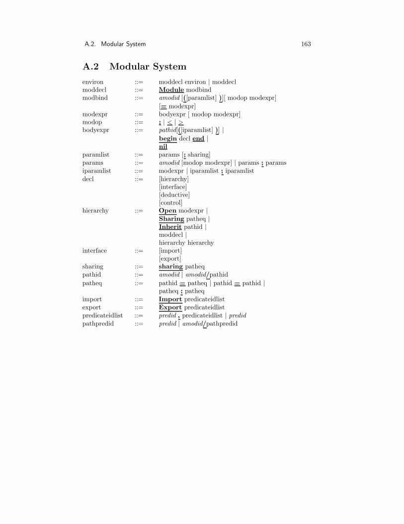
A.2. Modular System 163
A.2 Modular System
environ ::= moddecl environ | moddeclmoddecl ::= Module modbindmodbind ::= amodid [([paramlist] )][ modop modexpr]
[= modexpr]modexpr ::= bodyexpr [ modop modexpr]modop ::= : | < | >bodyexpr ::= pathid[([iparamlist] )] |
begin decl end |nil
paramlist ::= params [; sharing]params ::= amodid [modop modexpr] | params ; paramsiparamlist ::= modexpr | iparamlist ; iparamlistdecl ::= [hierarchy]
[interface][deductive][control]
hierarchy ::= Open modexpr |Sharing patheq |Inherit pathid |moddecl |hierarchy hierarchy
interface ::= [import][export]
sharing ::= sharing patheqpathid ::= amodid | amodid/pathid
patheq ::= pathid = patheq | pathid = pathid |patheq ; patheq
import ::= Import predicateidlistexport ::= Export predicateidlistpredicateidlist ::= predid , predicateidlist | predidpathpredid ::= predid | amodid/pathpredid

164 Appendix A. Syntax of Milord II
A.3 Deductive Knowledge
deductive ::= Deductive knowledge[Dictionary: dictionary][Rules: rules][Inference system: logcomp]end deductive
A.3.1 Dictionary
dictionary ::= [typedef] preddeftypedef ::= Types: typebindingstypebindings ::= typeid [= [temporal] typespec] |
typebindings typebindingstypespec ::= (values )|
predefined |typeid |Array [ arraydim ] |
Set Of typeid |frame framespec end frame
predefined ::= boolean | logic | numeric | classarraydim ::= typeid |
numeric |arraydim , arraydim
framespec ::= slotid : typeidframespec framespec
preddef ::= Predicates: predbindingspredbindings ::= predid = attributes |
predbindings predbindingsattributes ::= name [question] type [function] [relations]name ::= Name: stringquestion ::= Question: stringtype ::= Type: [temporal] typespecfunction ::= Function: S-expressionrelations ::= Relation: relationid pathpredid |
relations relationsrelationid ::= predef-rel-id | symbolpredef-rel-id ::= Needs | Needs true |
Needs false | Belongs to
A.3.2 Rules
rules ::= rule rules | rulerule ::= ruleid If premisse-rule Then conclusion-rule
[documentation]premisse-rule ::= condition-rule and premisse-rule | condition-rule

A.3. Deductive Knowledge 165
conclusion-rule ::= conclude rconclusion is cert-valuecondition-rule ::= conditio |
no (conditio )
rconclusion ::= form |elemental = (values )|
no (elemental )|
no (form op form )|
no (elemental = (values ))
form ::= elemental | (form op form )
elemental ::= predid | varidvalues ::= symbol , values | symbolvalues1 ::= symbol between [ ltermid , ltermid] , values1 |
symbol between [ ltermid , ltermid]
conditio ::= operator (expression, ..., expression )|
pathform | cert-value |expression operator expression
pathform ::= pathform-s | pathform-cpathform-s ::= elemental | amodid/pathform-s | varid/pathform-s
pathform-c ::= (formula )| amodid/pathform-c | varid/pathform-c
formula ::= (pathform op pathform )
expression ::= operator-arit (expression, ..., expression )|
(expression operator-arit expression )|
numeric | elemental | pathpredid | pathvar |values | values1
S-expression ::= atom | list | S-expression S-expressionlist ::= (S-expression )| ()
operator ::= < | > | <= | >= | = | /= | int
operator-arit ::= + | - | * | : | symbol

166 Appendix A. Syntax of Milord II
A.4 Inference System
logcomp ::= [lingtermdef] [order][renaming][connectives][infpat]
lingtermdef ::= Truth values = (ltermidlist )|
Truth values = (ltermlist )
ltermidlist ::= ltermid , ltermidlist | ltermidltermlist ::= ltermid = (real, real, real, real ), ltermlist |
ltermid = (real, real, real, real)
cert-value ::= ltermid |number |[ ltermid , ltermid] |
[number , number] |
(certarrows )
certarrows ::= certlist |(certarrows )certarrows
certlist ::= ltermid |number |certlist certlist
renaming ::= Renaming lrenameslrenames ::= pathid/cert-value ==> cert-value lrenames |
pathid/cert-value ==>cert-value |
S-expressionconnectives ::= Connectives:
[Negation = fundef][Conjunction = fundef][Disjunction = fundef]
infpat ::= Inference patterns:Modus ponens = fundef
fundef ::= S-expression | fileid | luckasiewicz |Zadeh | probabilistic | truth-table
order ::= (ltermid, ltermid) order |
λtruth-table ::= Truth table (arrows)
arrows ::= (termlist) | arrows arrows
ltermlist ::= ltermid | ltermlist ltermlist

A.5. Control Knowledge 167
A.5 Control Knowledge
control ::= Control knowledge[search] [threshold][deduccnt] [structcnt]end control
A.5.1 Evaluation Type
search ::= Evaluation type: evaltypeevaltype ::= lazy | eager | heuristic | input | reified
A.5.2 Truth Threshold
threshold ::= Truth threshold: cert-value
A.5.3 Deductive Control
deduccnt ::= Deductive control: lmrrlmrr ::= mrr lmrr | mrrmrr ::= metaid If premisse-meta Then filters-mrrfilters-mrr ::= filter-mrr filters-mrr | filter-mrrpremisse-meta ::= condition-meta and premisse-meta |
condition-metacondition-meta ::= mconditio |
no(mconditio )|
mconditio ::= metapredid (conditionterm , ..., conditionterm )
conditionterm ::= operation (conditionterm ,..., conditionterm )|
metafunctid (conditionterm , ..., conditionterm )|
conditiofilter-mrr ::= inhibit rules relation-id pathpredid |
inhibit rules pathpredid |prune pathpredid |increase form integer |decrease form integer |conclusion-meta
conclusion-meta ::= mconclusion |no (mconclusion )
mconclusion ::= metapredid (conclusionterm , ..., conclusionterm )
conclusionterm ::= operation (conclusionterm , ..., conclusionterm )|
metafunctid (conclusionterm ,..., conclusionterm )|
form
A.5.4 Structural Control
structcnt ::= Structural control: lmrelmre ::= mre | mrx | lmre lmre

168 Appendix A. Syntax of Milord II
mre ::= metaid If premisse-meta Then filter-mrefilter-mre ::= filter amodidlist |
order amodidlist with certainty cert-value |Open (conclusionterm , ..., conclusionterm )|
Module (conclusionterm , ..., conclusionterm )|
Inherit (conclusionterm , ..., conclusionterm )
amodidlist ::= amodid amodidlist | amodidmrx ::= metaid If premisse-meta Then exceptionexception ::= definitive solution predid |
stop

Appendix B
Proofs
Proposition B.1 MP ∗T ([a, b], [c, 1]) = [T (a, c), 1]
Proof. It reduces to find all solutions of the functional inequations
IT (x, z) ≥ c
being a ≤ x ≤ b. However, given a residuated pair (T, IT ) it is well known thatthe following relation holds:
T (x, y) ≤ z iff IT (x, z) ≥ y
Then, the solution for the first equation is z ≥ T (x, c), and taking into accountthat x ≥ a, and that z = 1 is always a solution, the minimal interval that willcontain all the solutions for z is [T (a, c), 1].2
B.1 Proposition
Proposition B.2 If p, q, p1, . . . , pn denote literal symbols then the followingproperties are fulfilled:
SR1: (p, V ) |= (p,W ) ⇔ V ⊆ W
SR2: (p, V ) |= (¬p,W ) ⇔ N ∗n(V ) ⊆ W
SR3: (p, V ), (p,W ) |= (p,U) ⇔ V ∩ W ⊆ U
SR4: (pi, Vi), (p1 ∧ · · · ∧ pn → q, V ) |= (p1∧· · ·∧pi−1∧pi+1∧· · ·∧pn → q,W ) ⇔MP ∗
T (Vi, V ) ⊆ W
SR5: MP ∗T (T ∗(V1, . . . , Vn),W ) =
MP ∗T (V1,MP ∗
T (V2, . . . ,MP ∗T (Vn,W ) . . .)), if W = [w, 1]
Finally we explain the proof of the properties:
169

170 Appendix B. Proofs
SR1: Straightforward from the satisfaction relation definition.
SR2: Follows from SR1 and the fact that a valuation ρ satisfies ρ(p) ∈ V if,and only if, ρ(¬p) ∈ N∗
n(V ).
SR3: Straightforward from the satisfaction relation definition.
SR4: First we prove the property for the simplest Modus Ponens case, i.e.,
(p,U), (p → q, V ) |= (q,W ) iff MP ∗T (U, V ) ⊆ W
By definition of the function MP ∗T , MP ∗
T (U, V ) is the minimal intervalcontaining all the solutions for ρ(q) in the following family of functionalequation systems:
ρ(p) = aρ(p → q) = IT (ρ(p), ρ(q)) = b
for any a ∈ U , and b ∈ V . Thus, for any model ρ satisfying ρ(p) ∈ U ,and ρ(p → q) ∈ V and ρ(q) ∈ W , it must be only the case that ρ(p) ∈MP ∗
T (U, V ), and thus MP ∗T (U, V ) ⊆ W . Moreover, if U = [x, y] and
V = [z, 1], then MP ∗T (U, V ) = [T (x, z), 1].
Now property SR4 follows straightforward from the associativity of the t-norm T , used to interpret conjunctions, and from the fact that a residuatedpair (T, IT ) satisfies the following equality:
IT (T (x, y), z) = IT (x, IT (y, z))
SR5: From proposition 1, it follows that, if U = [x, y] and V = [z, 1], thenMP ∗
T (U, V ) = [T (x, z), 1]. Then, it is easy to see that, due to the associa-tivity of the t-norm T , if Vi = [ai, bi], for i = 1, . . . , n, then
T ∗(V1, . . . , Vn) = [T (a1, . . . , an)1, T (b1, . . . , bn)]
and thus, on the one hand
MP ∗T (V1,MP ∗
T (V2, . . . ,MP ∗T (Vn,W ) · · ·)) = [T (a1, . . . , T (an, w) · · ·), 1]
= [T (a1, . . . , an, w), 1]
and on the other hand
MP ∗T (T ∗(V1, . . . , Vn),W ) = MP ([T (a1, . . . , an), T (b1, . . . , bn)], [w, 1])
= [T (a1, . . . , an, w), 1]
Properties from SR1 to SR4 give us a foundation for the specialization cal-culus.
1The expression T (r1, r2, r3, . . .) is the recurrent application of T as T (r1, T (r2, T (r3 . . .) . . .)

B.2. Soundness Theorem 171
B.2 Soundness Theorem
From properties SR1, SR2, SR3 and SR4 of the semantical entailment, it is easyto check that the above specialization calculus is sound.
Theorem B.1 (Soundness) Let A be a sentence and Γ a set of sentences.Then Γ ` A implies Γ |= A
Proof. The properties SR1-SR4 show that the inference rules are locallysound and complete. So, we need only to show that the axioms are sound tohave the proof of the theorem.
1. If A is the axiom AS1, i.e. A = (¬¬p → p, [1, 1]) then for every modelMρ, ρ(p) = N(N(ρ(p))) = N(ρ(¬p)) = ρ(¬(¬(p))) ⇒ I(¬¬p → p) =I(ρ(¬¬p), ρ(p)) = 1. Then, for all Mρ, Mρ |= (¬¬p → p, [1, 1]).
2. If A is the axiom AS2, i.e. A = (p, [0, 1]), it is the case that every modelMρ satisfies ρ(p) ∈ [0, 1]. Then for all Mρ, we have trivially that Mρ |=(p, [0, 1]).
3. If A is the axiom A1, i.e., A = (true, [1, 1]) then, by definition, for everymodel Mρ, ρ(true) = 1 ⇒ Mρ |= (true, [1, 1]).
4. If A is the axiom A2, the proof is analogous to the previous case.
B.3 Restricted Completeness
B.3.1 Literal Completeness
It is straightforward to see that our deductive system is not complete. Forinstance, we have (p → q, 1), (q → r, 1) |= (p → r, 1) but (p → q, 1), (q →r, 1) 6` (p → r, 1). It is also the case that the language is not complete for literaldeduction in general. For instance, we have (p → q, 1), (¬p → q, 1) |= (q, 1)but (p → q, 1), (¬p → q, 1) 6` (q, 1). However, it can be proved that the systemis complete for literal deduction in the context of a restricted language setting,as it will be shown in this section.
Previous definitions
Definition B.1 (Mv-Horn-Rules) We define the set Mv-Horn-Rules as theset (p1 ∧ p2 ∧ · · · ∧ pn → q, V ) | pi and q are atomic symbols, V = [a, 1] is aninterval of truth-values of An with a > 0, and ∀i, j(pi 6= pj , q 6= pj)
Definition B.2 (Restricted Language) Given the propositional language
Ln = (An, Σ, C,Sn)
we define a restricted propositional language as:
RLn = (An, Σ, C,RSn)

172 Appendix B. Proofs
where RSn = Mv-Atoms ∪ Mv-Horn-Rules
For any Γ ⊂ RSn the next notation will be used:
• Γ = ΓL ∪ ΓR
• ΓL = γ ∈ Γ|γ are mv-Atoms
• ΓR = γ ∈ Γ|γ are mv-Horn-Rules
• Prem: Is a function that given a rule returns its conditions.
• Cond: Is a function that given a rule returns its conclusion.
• ΓAL = p ∈ Σ|∃V interval of An : (p, V ) ∈ ΓL
• ΓAR = p ∈ Σ|∃r ∈ ΓR : p ∈ Prem(r) or p = Concl(r)
• ΓA = ΓAL ∪ ΓA
R
Previous Lemmas
Proposition B.3 The inference rules (Weakening, Composition, Negation andSpecialization) are locally complete, i.e., they verify the following equivalences:
1. (p, V ) ` (p,W ) iff (p, V ) |= (p,W )
2. (p, V ) ` (¬p,W ) iff (p, V ) |= (¬p,W )
3. (p, V ), (p,W ) ` (p,U) iff (p, V ), (p,W ) |= (p,U)
4. (p1, V1), . . . , (pn, Vn), (p1 ∧ · · · ∧ pn → q,W ) ` (q, U) iff (p1, V1), . . . ,(pn, Vn), (p1 ∧ · · · ∧ pn → q,W ) |= (q, U)
Proof. Straightforward from properties SR1-SR5 and from the definition ofthe four inference rules in Section 3.3.
Lemma B.1 Let ΓL be a set of Mv-Atoms, and let R1, R2 be two sets of mv-Horn-Rules. R1 and R2 rules have as premises conjunctions of atoms belongingto ΓA
L , and share the same conclusion, an atom p not belonging to Γ AL .
If V1 =⋂
V ′′|ΓL, R1 |= (p, V ′′), V2 =⋂
V ′′|ΓL, R2 |= (p, V ′′) andW =
⋂
V ′′|ΓL, R1, R2 |= (p, V ′′), then W ⊇ V1 ∩ V2.
Proof. By reductio ad absurdum. Suppose that W 6⊇ V1 ∩ V2. Then ∃α ∈V1 ∩ V2 and α 6∈ W . Because of V1 and V2 are minimals, we have that:
• α ∈ V1 ⇒ ∃Mρ such that ρ(p) = α, Mρ |= ΓL and Mρ |= R1
• α ∈ V2 ⇒ ∃Mρ′ such that ρ′(p) = α, Mρ′ |= ΓL and Mρ′ |= R2

B.3. Restricted Completeness 173
We will prove that there always exists a model Mρ′′ such that ρ′′(p) = α,Mρ′′ |= ΓL, Mρ′′ |= R1 and Mρ′′ |= R2. Define ρ′′(p) = α, and ρ′′(a) =min(ρ(a), ρ′(a)), ∀a ∈ ΓA
L . Mρ′′ easily extends to the Mv-Horn-Rules by theimplication function IT . Then, for this model Mρ′′ we have:
1. ρ′′(p) = α.
2. Mρ′′ |= ΓL: due to the fact that ρ′′ = min(ρ, ρ′) over ΓAL .
3. Mρ′′ |= R1: ∀r ∈ R1, where r = (q1 ∧ · · · ∧ qm → p, [vr, 1]), we have thatMρ |= R1 implies ρ(r) ≥ vr . Given that we work with Mv-Horn rules, i.e.qi are not negated literals, and the monotonicity property of function T ,it always holds that:
ρ′′(q1 ∧ · · · ∧ qn) =
T (ρ′′(q1), . . . , ρ′′(qn)) ≤ T (ρ(q1), . . . , ρ(qn)) = ρ(q1 ∧ · · · ∧ qn)
and, given that IT is not increasing in the first argument, it always holdsthat:
ρ′′(r) = IT (ρ′′(q1 ∧ · · · ∧ qn), α) ≥ IT (ρ(q1 ∧ · · · ∧ qn), α) = ρ(r) ≥ vr
that is, M ′′ρ |= R1.
4. Mρ′′ |= R2: Analogously to the previous case.
Summarizing, we have found Mρ′′ such that ρ′′(p) = α, Mρ′′ |= ΓL, Mρ′′ |=R1 and Mρ′′ |= R2, i.e. ΓL, R1, R2 6|= (p,W ) which is in contradiction withthe enunciate of the lemma.2
Next Lemma shows that previous deductions over a Mv-Atom p do not re-strict the models of Mv-Atoms belonging to premises of other rules concludingthe same Mv-Atom p. In practical terms, having previous deductions over anatom r means that we know r with an interval of truth values of type [v, 1].Otherwise, if we knew r with a general interval of type [b, c] it could be the casethat premises of rules concluding r would be semantically deduced with inter-vals different of [0, 1]. On the contrary, it would not be possible to syntacticallydeduce them. So, next Lemma allows us, when considering atom deducibility,to only consider those rules that deduce it and not the rules that use it as apremise.
Lemma B.2⋂
V ′′|(p ∧ q1 ∧ · · · ∧ qn → r, [a, 1]), (r, [b, 1]) |= (p, V ′′) = [0, 1]
Proof. It is sufficient to prove that ∀α ∈ [0, 1], we can find a model Mρ suchthat ρ(p) = α and that Mρ |= (p ∧ q1 ∧ · · · ∧ qn → r, [a, 1]) and Mρ |= (r, [b, 1]).Actually, every model Mρ such that ρ(p) = α and ρ(r) = 1, satisfies thatρ(p ∧ q1 ∧ · · · ∧ qn → r) = 1, and thus Mρ |= (p ∧ q1 ∧ · · · ∧ qn → r, [a, 1])and Mρ |= (r, [b, 1]). 2

174 Appendix B. Proofs
B.3.2 Restricted Literal Completeness Theorem
Theorem B.2 (Restricted Literal Completeness) If Γ |= (p, V ), then Γ `(p, V ), provided that p ∈ ΓA, where Γ is such that the following conditions hold:
1. Γ ⊂ RSn
2. ∀r ∈ ΓR : concl(r) 6∈ ΓAL
3. The deductive and/or graph associated to Γ is acyclic.
Proof. Given that the and/or deductive graph associated to Γ is acyclic, wecan decompose the set ΓA of atomic symbols appearing in Γ in a set of disjointlayers. The definition of the layers is the following:
• S0 = q ∈ ΓA| 6 ∃r ∈ ΓR : Concl(r) = q
• S1 = q ∈ ΓA|∀r ∈ ΓR : Concl(r) = q ⇒ ∀x ∈ Prem(r), x ∈ S0
• ...
• Si = q ∈ ΓA|∀r ∈ ΓR : Concl(r) = q ⇒ ∀x ∈ Prem(r), x ∈ Sj , being j <i and ∃r : ∃x ∈ Prem(r), x ∈ Si−1
• ...
The proof of the theorem is by induction over the layer number n to which pbelongs. Suppose that V 6= [0, 1], otherwise the proof of the theorem is trivial.
The set ΓA is decomposed in layers ΓA =⋃
i=1,n Si. Because of Lemma 2, inorder to deduce p we only need to consider that part of Γ containing rules usingatoms belonging to layers lower than the layer of p. That is, we consider onlythose rules of Γ belonging to the deductive subgraph of p.
Case n = 0: In this case Γ contains a set of mv-atoms as
(p, Vi)|i ∈ I ⊆ ΓL
Then, it is easy to see that every model Mρ that satisfies Γ must holdρ(p) ∈ (
⋂
i∈I Vi), and then (⋂
i∈I Vi) ⊆ V . Therefore, we can assure thatif we apply repeatedly the composition and weakening rules, we also candeduce syntactically (p, V ). Then the theorem is true for n = 0.
Induction hypothesis: The theorem is true for n − 1.
Case n: Suppose that p ∈ Sn. Given Rp, the set of rules of Γ with conclusionp, then ∀r ∈ Rp, the premises of r belong to lower layers. Let be Vq =⋂
V |Γ |= (q, V ), ∀q ∈ Prem(r), ∀r ∈ Rp. By the induction hypothesiswe have that Γ |= (q, Vq) ⇒ Γ ` (q, Vq), ∀q ∈ Prem(r), ∀r ∈ Rp.
By induction over nrp, the number of rules of Rp, and together with theconditions of the theorem, we will prove that Γ |= (p, V ) implies Γ ` (p, V ).

B.3. Restricted Completeness 175
1. nrp = 1. In this case we have Rp = (q1 ∧ · · · ∧ qm → p,W ),Γ |= (qi, Vqi
) for i = 1, . . . ,m, where Vqiare minimals. From Lemma
2 we have that Γ |= (p, V ) if and only if
(q1 ∧ · · · ∧ qm → p,W )(q1, Vq1), . . . , (qm, Vqm
) |= (p, V )
but from properties SR-4 and SR-5 of proposition 2, this holds if andonly if
V ⊇ MP ∗T (T ∗(Vq1
, Vq2, . . . , Vqm
),W )
Given that
MP ∗T (T ∗(Vq1
, Vq2, . . . , Vqm
,W ) = MP ∗T (Vq1
,MP ∗T (Vq2
, . . . ,MP ∗
T (Vqm,W ) · · ·))
it is easy to see that by successive applications of SIR inference rulewe can obtain Γ ` (p, V ), and thus for nrp = 1 the theorem is true.
2. Suppose that the theorem is true for nrp = k − 1.
3. nrp = k. In this case we have that Rp = r1, r2, . . . , rk and Γ |=(qij ,Wqij
) for all qij ∈ Prem(ri), i = 1, . . . , k, being Wqijmini-
mal. Let be ri = (∧qij → p, Vi) and Ap =⋃
i,j(qij ,Wqij). Again
Lemma 2 allows us to state that Γ |= (p, V ) if and only if V ⊇ U ,where r1, . . . , rk ∪ Ap |= (p,U) and U minimal,. Consider Rp =R∗
p∪rk , where R∗p = r1, . . . , rk−1 and let be V ∗ =
⋂
V ′′|R∗p, Ap |=
(p, V ′′). By induction hypothesis we have also R∗p ` (p, V ∗). Fur-
thermore we have rk, Ap ` (p,MP ∗T (T ∗(Wqk1
, . . . ,Wqkjk, Vk)), and
because of Lemma 1 we know that MP ∗T (T ∗(Wqk1
, . . . ,Wqkjk, Vk) =
⋂
V ′′|rk, Ap |= (p, V ′′). Then from Lemma 1, we have:
Rp, Ap |= (p, V ) iff V ⊇ V ∗ ∩ MP ∗T (T ∗(Wqk1
, . . . ,Wqkjk, Vk)
Finally it is easy to notice that V ∗ ∩ MP ∗T (T ∗(Wqk1
, . . . ,Wqkjk, Vk)
can be obtained by successive applications of SIR and compositioninference rules, that is, we can finally conclude that Γ ` (p, V ).2

176 Appendix B. Proofs

Appendix C
Code Examples
C.1 Terap–IA Example
In the following we present an small selection of the code of Terap–IA that hasbeen explained in Section 6.2.
;; 17-3-93
;; MODULS DE TRACTAMENT DE LES PNEUMONIES ATIPIQUES
Module pneumonia_chlam_pneum_tractament_1: antibiotics_chlamydia_pneum =
Begin
Inherit ant
Inherit situacio_clinica
Open insuf_renal:
Begin
Export quinol, tetras_1, tetras_2, macrol
End
Export cipro, oflox, tetras_ac_rap, doxi, doxi_DI,
eritro_DB, eritro_DA, roxi
Deductive Knowledge
Rules:
;; quinolones per chlamydia_pneum
R004 If quinol then conclude cipro is modp
R005 If quinol and situacio_clinica/tract_OR then conclude oflox is p
;;tetraciclines per chlamydia_pneum
R006 If tetras_1 then conclude tetras_ac_rap is mp
R007 If tetras_2 then conclude doxi is mp
R008 If tetras_2 then conclude doxi_DI is mp
;; macrolids per chlamydia_pneum
R001 If macrol then conclude eritro_DB is fp
R002 If macrol then conclude eritro_DA is fp
R003 If macrol and situacio_clinica/tract_OR then conclude roxi is p
End deductive
End
;;-------------------------------
;; Atmar RL, Greenberg SB, Pneumonia caused by Mycoplasma
;; pneumoniae and the TWAR Agent. Semin Respir Infect 1989; 4:
;; l9-31
177

178 Appendix C. Code Examples
;; Grayston JT, Wang SP, Kuo CC,Campbell LA, Current knowledge
;; on Chlamydia Pneumoniae , strain TWAR, an important cause of
;; pneumonia and other acute respiratory diseases. Eur J Clin
;; Microbiol Infect Dis 1989; 8: 191-202
;; Lipski BA, Tack KJ, Kuo C, Wang S, Grayston T. Ofloxacin
;; treatment of Chlamydia Pneumoniae (Strain TWAR) Lower
;; Respiratory Tract Infections. Am J Med 1990,89: 722-724
;; Grayston JT, Thom DH. The chlamydial pneumonias, in Remington
;; JS, Swartz MN. Current Clinical Topics in Infectious Diseases.
;; Boston, Blackwell Scientific Publications, 1991: 1-18
;; Finegold SM. Aspiration Pneumonia, Lung abscess and Empiema.
;; Pennington JE. Respiratory Infections: Diagnosis and Management.
;; Raven Press, New York 1988: 264_275
;;--------------------------------
Module antibiotics_chlamydia_pneum=antimicrobians:
Begin
Export cipro, oflox, tetras_ac_rap, doxi, doxi_DI, eritro_DB,
eritro_DA, roxi
End
Module ABS=
;; MODUL ABS GRUPS D’ANTIMICROBIANS QUE S’UTILITCEN A TERAPIA
Begin
Export quinol, tetras_1, tetras_2, cotri, sulfas, vanco, teico, amino,
metro, clinda, carbapen, INH, RFM, ETM, PZ, anf_B, ACV, GCV,
ARA_A, RBV, AMD, RMD, peni, macrol, b_lactam_inh, cef, monobac
Deductive knowledge
Dictionary:
Predicates:
quinol= name: "quinolones"
type: logic
tetras_1= name: "tetraciclines d’accio rapida"
type: logic
relation: belongs_to_group tetraciclines
tetras_2= name: "tetraciclines de accio retardada"
type: logic
relation: belongs_to_group tetraciclines
cotri= name: "cotrimoxazol"
type: logic
sulfas= name: "sulfamidas"
type: logic
vanco= name: "vancomicina"
type: logic
teico= name: "teicoplanina"
type: logic
amino= name: "aminoglucosids"
type: logic
metro= name: "metronidazol"
type: logic
clinda= name: "clindamicina"
type: logic

C.1. Terap–IA Example 179
carbapen= name: "carbapenems"
type: logic
relation: belongs_to_group atb_betalactamics
INH= name: "isoniacida"
type: logic
relation: belongs_to_group tuberculostatics
RFM= name: "rifampicina"
type: logic
relation: belongs_to_group tuberculostatics
ETM= name: "etambutol"
type: logic
relation: belongs_to_group tuberculostatics
PZ= name: "pirazinamida"
type: logic
relation: belongs_to_group tuberculostatics
anf_B= name: "anfotericina_B"
type: logic
ACV= name: "aciclovir"
type: logic
relation: belongs_to_group antivirics
GCV= name: "ganciclovir"
type: logic
relation: belongs_to_group antivirics
ARA_A= name: "vidarabina"
type: logic
relation: belongs_to_group antivirics
RBV= name: "ribaravina"
type: logic
relation: belongs_to_group antivirics
AMD= name: "amantadina"
type: logic
relation: belongs_to_group antivirics
RMD= name: "rimantadina"
type: logic
relation: belongs_to_group antivirics
peni= name: "penicil.lines"
type: logic
relation: belongs_to_group atb_betalactamics
macrol= name: "macrolids"
type: logic
b_lactam_inh= name: "inhibidors de les betalactamases"
type: logic
relation: belongs_to_group atb_betalactamics
cef= name: "cefalosporines"
type: logic
relation: belongs_to_group atb_betalactamics
monobac= name: "monobactams"
type: logic
relation: belongs_to_group atb_betalactamics
atb_betalactamics= name: "antibiotics betalactamics"
type:class
tetraciclines name: "tetraciclines"
type: class
antivirics= name: "farmacs antivirics"
type: class
tuberculostatics= name: "agents antituberculosos"
type: class

180 Appendix C. Code Examples
End deductive
End
;; 18-3-93
;;----------------------DOCUMENT CONDICIONS GENERALS--------------
;; EL MODUL ABS_1 ES UN REFINAMENT DEL MODUL ABS (VEURE
;; DOCUMENT DIC) EN EL QUE ES DONA UN VALOR DE CERTESA SEGUR A
;; TOTS ELS GRUPS D’ANTIBIOTICS UTILITZATS A TERAP-IA
Module ABS_1:ABS =
Begin
Export quinol, tetras_1, tetras_2, cotri, sulfas, vanco, teico, amino,
metro, clinda, carbapen, INH, RFM, ETM, PZ, anf_B, ACV, GCV,
ARA_A, RBV, AMD, RMD, peni, macrol, b_lactam_inh, cef, monobac
Deductive Knowledge
Rules:
R001 If s then conclude quinol is s
R002 If s then conclude tetras_1 is s
R003 If s then conclude tetras_2 is s
R004 If s then conclude cotri is s
R005 If s then conclude sulfas is s
R006 If s then conclude vanco is s
R007 If s then conclude teico is s
R008 If s then conclude amino is s
R009 If s then conclude metro is s
R010 If s then conclude clinda is s
R011 If s then conclude carbapen is s
R012 If s then conclude INH is s
R013 If s then conclude RFM is s
R014 If s then conclude ETM is s
R015 If s then conclude PZ is s
R016 If s then conclude anf_B is s
R017 If s then conclude ACV is s
R018 If s then conclude GCV is s
R019 If s then conclude ARA_A is s
R020 If s then conclude RBV is s
R021 If s then conclude AMD is s
R022 If s then conclude RMD is s
R023 If s then conclude peni is s
R024 If s then conclude macrol is s
R025 If s then conclude b_lactam_inh is s
R026 If s then conclude cef is s
R027 If s then conclude monobac is s
R028 If s then conclude (macrol plus RFM) is s
R029 If s then conclude (peni plus metro) is s
R030 If s then conclude (macrol plus metro) is s
End deductive
End
;; ELS MODULS GESTACIO, LACTANCIA, ALERGIA, INSUFICIENCIA RENAL I
;; FACTORS GENETICS SON MODULS DE CONDICIONS GENERALS DEL
;; PACIENT QUE MODIFIQUEN LA TERAPIA I QUE ES PODEN APLICAR SOBRE
;; GRUPS D’ANTIBIOTICS. CADA UNA D’AQUESTES CONDICIONS AFECTEN
;; PER IGUAL A TOTS ELS ANTIBIOTIC DE UN MATEIX GRUP I PER TANT ES
;; PODEN APLICAR SOBRE EL GRUP
Module insuf_renal:ABS=

C.1. Terap–IA Example 181
Begin
Module x = alergia
;; anam_R es un refinament d’anam per insuficiencia renal
Module anam_R= anam:
Begin
Export insuf_renal
End
Export quinol, tetras_1, tetras_2, cotri, sulfas, vanco, teico, amino,
metro, clinda, carbapen, INH, RFM, ETM, PZ, anf_B, ACV, GCV,
ARA_A, RBV, AMD, RMD, peni, macrol, b_lactam_inh, cef, monobac
Deductive Knowledge
Rules:
R001 If anam_R/insuf_renal then conclude no(tetras_1) is s
R002 If anam_R/insuf_renal then conclude tetras_2 is p
R003 If anam_R/insuf_renal then conclude amino is p
R004 If anam_R/insuf_renal then conclude anf_B is p
R005 If anam_R/insuf_renal then conclude AMD is p
End Deductive
Control knowledge
Evaluation type: eager
Deductive control:
M001 If K(x/$y,$c) and NP($y) then conclude K($y,$c)
End control
End
Module Alergia:ABS=
Begin
Module x = lactancia
;; anam_R es anam refinat per alergia
Module anam_R= anam:
Begin
Export alergia, alergia_grups_ABS, alergia_inmed_peni,
alergia_retard_peni, alergia_infrec
End
Export quinol, tetras_1, tetras_2, cotri, sulfas, vanco, teico, amino,
metro, clinda, carbapen, INH, RFM, ETM, PZ, anf_B, ACV, GCV,
ARA_A, RBV, AMD, RMD, peni, macrol, b_lactam_inh, cef, monobac
Deductive Knowledge
Rules:
R001 If anam_R/alergia_grups_ABS=(quinol) then conclude no(quinol) is s
R002 If anam_R/alergia_grups_ABS=(tetras_1)
then conclude no(tetras_1) is s
R003 If anam_R/alergia_grups_ABS=(tetras_2)
then conclude no(tetras_2) is s
R004 If anam_R/alergia_grups_ABS=(cotri) then conclude no(cotri) is s
R005 If anam_R/alergia_grups_ABS=(sulfas) then conclude no(cotri) is s
R006 If anam_R/alergia_grups_ABS=(sulfas) then conclude no(sulfas) is s
R007 If anam_R/alergia_grups_ABS=(vanco) then conclude no(vanco) is s
R008 If anam_R/alergia_grups_ABS=(teico) then conclude no(teico) is s
R009 If anam_R/alergia_grups_ABS=(vanco) then conclude teico is llp
R010 If anam_R/alergia_grups_ABS=(amino) then conclude no(amino) is s
R011 If anam_R/alergia_grups_ABS=(metro) then conclude no(metro) is s
R012 If anam_R/alergia_grups_ABS=(clinda) then conclude no(clinda) is s
R013 If anam_R/alergia_grups_ABS=(carbapen) then conclude no(carbapen) is s
R014 If anam_R/alergia_inmed_peni then conclude no(carbapen) is s
R015 If anam_R/alergia_retard_peni then conclude carbapen is p
R016 If anam_R/alergia_infrec then conclude carbapen is p

182 Appendix C. Code Examples
R017 If anam_R/alergia_grups_ABS=(INH) then conclude no(INH) is s
R018 If anam_R/alergia_grups_ABS=(RFM) then conclude no(RFM) is s
R019 If anam_R/alergia_grups_ABS=(ETM) then conclude no(ETM) is s
R020 If anam_R/alergia_grups_ABS=(PZ) then conclude no(PZ) is s
R021 If anam_R/alergia_grups_ABS=(anf_B) then conclude no(anf_B) is s
R022 If anam_R/alergia_grups_ABS=(ACV) then conclude no(ACV) is s
R023 If anam_R/alergia_grups_ABS=(GCV) then conclude no(GCV) is s
R024 If anam_R/alergia_grups_ABS=(ARA_A) then conclude no(ARA_A) is s
R025 If anam_R/alergia_grups_ABS=(RBV) then conclude no(RBV) is s
R026 If anam_R/alergia_grups_ABS=(AMD) then conclude no(AMD) is s
R027 If anam_R/alergia_grups_ABS=(RMD) then conclude no(RMD) is s
R028 If anam_R/alergia_grups_ABS=(peni) then conclude no(peni) is s
R029 If anam_R/alergia_grups_ABS=(macrol) then conclude no(macrol) is s
R030 If anam_R/alergia_grups_ABS=(b_lactam_inh)
then conclude no(b_lactam_inh) is s
R031 If anam_R/alergia_grups_ABS=(peni)
then conclude no(b_lactam_inh) is s
R032 If anam_R/alergia_grups_ABS=(cef) then conclude no(cef) is s
R033 If anam_R/alergia_inmed_peni then conclude no(cef) is s
R034 If anam_R/alergia_retard_peni then conclude cef is p
R035 If anam_R/alergia_infrec then conclude cef is p
R036 If anam_R/alergia_grups_ABS=(monobac)
then conclude no(monobac) is s
R037 If anam_R/alergia_grups_ABS=(metro)
then conclude no(peni plus metro) is s
R038 If anam_R/alergia_grups_ABS=(peni)
then conclude no(peni plus metro) is s
R039 If anam_R/alergia_grups_ABS=(macrol)
then conclude no(macrol plus metro) is s
R040 If anam_R/alergia_grups_ABS=(metro)
then conclude no(macrol plus metro) is s
R041 If anam_R/alergia_grups_ABS=(RFM)
then conclude no(macrol plus RFM) is s
R042 If anam_R/alergia_grups_ABS=(macrol)
then conclude no(macrol plus RFM) is s
End Deductive
Control knowledge
Evaluation type: eager
Deductive control:
M001 If K(x/$y,$c) and NP($y) then conclude K($y,$c)
End control
End
;; LACTANCIA NO MODIFICA EL VALOR DELS GRUPS
;; D’ANTIBIOTICS. SI UN ANTIBIOTIC NO ESTA RECOMANAT EN LA
;; LACTANCIA S’ACONSELLA DEIXAR DE LACTAR.
Module lactancia:ABS=
;; falta posar bibliografia
Begin
Module X = gestacio
Module AD = anam_dona
Export quinol, tetras_1, tetras_2, cotri, sulfas, vanco, teico, amino,
metro, clinda, carbapen, INH, RFM, ETM, PZ, anf_B, ACV, GCV,
ARA_A, RBV, AMD, RMD, peni, macrol, b_lactam_inh, cef, monobac
Deductive knowledge
Dictionary:
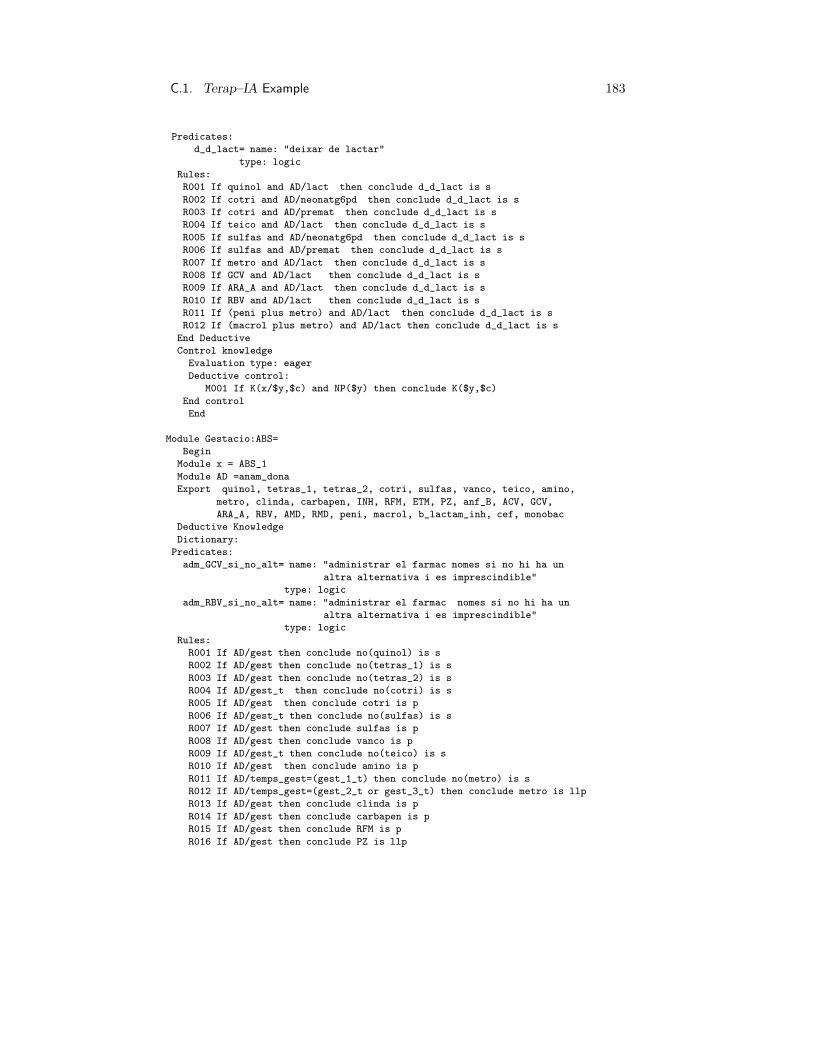
C.1. Terap–IA Example 183
Predicates:
d_d_lact= name: "deixar de lactar"
type: logic
Rules:
R001 If quinol and AD/lact then conclude d_d_lact is s
R002 If cotri and AD/neonatg6pd then conclude d_d_lact is s
R003 If cotri and AD/premat then conclude d_d_lact is s
R004 If teico and AD/lact then conclude d_d_lact is s
R005 If sulfas and AD/neonatg6pd then conclude d_d_lact is s
R006 If sulfas and AD/premat then conclude d_d_lact is s
R007 If metro and AD/lact then conclude d_d_lact is s
R008 If GCV and AD/lact then conclude d_d_lact is s
R009 If ARA_A and AD/lact then conclude d_d_lact is s
R010 If RBV and AD/lact then conclude d_d_lact is s
R011 If (peni plus metro) and AD/lact then conclude d_d_lact is s
R012 If (macrol plus metro) and AD/lact then conclude d_d_lact is s
End Deductive
Control knowledge
Evaluation type: eager
Deductive control:
M001 If K(x/$y,$c) and NP($y) then conclude K($y,$c)
End control
End
Module Gestacio:ABS=
Begin
Module x = ABS_1
Module AD =anam_dona
Export quinol, tetras_1, tetras_2, cotri, sulfas, vanco, teico, amino,
metro, clinda, carbapen, INH, RFM, ETM, PZ, anf_B, ACV, GCV,
ARA_A, RBV, AMD, RMD, peni, macrol, b_lactam_inh, cef, monobac
Deductive Knowledge
Dictionary:
Predicates:
adm_GCV_si_no_alt= name: "administrar el farmac nomes si no hi ha un
altra alternativa i es imprescindible"
type: logic
adm_RBV_si_no_alt= name: "administrar el farmac nomes si no hi ha un
altra alternativa i es imprescindible"
type: logic
Rules:
R001 If AD/gest then conclude no(quinol) is s
R002 If AD/gest then conclude no(tetras_1) is s
R003 If AD/gest then conclude no(tetras_2) is s
R004 If AD/gest_t then conclude no(cotri) is s
R005 If AD/gest then conclude cotri is p
R006 If AD/gest_t then conclude no(sulfas) is s
R007 If AD/gest then conclude sulfas is p
R008 If AD/gest then conclude vanco is p
R009 If AD/gest_t then conclude no(teico) is s
R010 If AD/gest then conclude amino is p
R011 If AD/temps_gest=(gest_1_t) then conclude no(metro) is s
R012 If AD/temps_gest=(gest_2_t or gest_3_t) then conclude metro is llp
R013 If AD/gest then conclude clinda is p
R014 If AD/gest then conclude carbapen is p
R015 If AD/gest then conclude RFM is p
R016 If AD/gest then conclude PZ is llp

184 Appendix C. Code Examples
R017 If AD/gest then conclude anf_B is p
R018 If AD/gest then conclude ACV is p
R019 If AD/gest then conclude GCV is llp
R020 If AD/gest then conclude no(ARA_A) is s
R021 If AD/gest then conclude RBV is llp
R022 If AD/gest then conclude no(AMD) is s
R023 If AD/gest then conclude RMD is llp
R024 If AD/gest then conclude (macrol plus RFM) is p
R025 If AD/temps_gest=(gest_1_t)
then conclude no(peni plus metro) is s
R026 If AD/temps_gest=(gest_2_t or gest_3_t)
then conclude (peni plus metro) is llp
End Deductive
Control knowledge
Evaluation type: eager
Deductive control:
M001 If K(x/$y,$c) and NP($y) then conclude K($y,$c)
End control
End
;;18-3-93
;;------------------------------MODULS MENU-------------------------
;; ELS MODULS QUE ANOMENO "MENU" SON MODULS DE PREGUNTES AL
;; USUARI DE LES DADES DEL MALALT QUE AJUDEN A DECIDIR EL
;; TRACTAMENT DE LES PNEUMONIES INCLOU EL MODUL DIAG QUE
;; PREGUNTA AL USUARI QUINS GERMENS VOL TRACTAR
MODULE DIAG=
;; DIAG PREGUNTA AL USUARI QUINS GERMENS VOL TRACTAR
;; pendent demanar la certesa del diag de un altra forma
Begin
Import diagnostics, pneum_leg, pneum_asper, pneum_tbc
Export diagnostics, pneum_leg, pneum_asper, pneum_tbc
Deductive Knowledge
Dictionary:
Predicates:
diagnostics=
name: "diagnostics"
question: "quina de les seguents vol tractar"
type: (pneum_myc or pneum_cox or pneum_chlam_psit or pneum_chlam_pneum
or pneum_leg or pneum_pneum or pneum_anaer or pneum_enterobac or
pneum_H_inf or pneum_branh or pneum_pseud or pneum_meningo or
pneum_S_pyog or pneum_S_aur or pneum_asper or pneum_crip
or pneum_nocar or pneum_CMV or pneum_VVZ or pneum_HSV or pneum_EBV
or pneum_VRS or pneum_ADV or pneum_influenza)
pneum_leg= name: "pneumonia per legionella pneumophila"
question: "quina es la certesa de pneum_leg"
type: logic
pneum_asper= name: "pneumonia per aspergilus"
question: "quina es la certesa de pneum_aspergilus"
type: logic
pneum_tbc= name: "pneumonia tuberculosa"
question: "quina es la certesa de pneum_myc_tuberculosis"
type: logic
End deductive
End

C.1. Terap–IA Example 185
MODULE ANAM_GENERAL=
;; ES UN MODUL EN EL QUE ES DEFINEIXEN LES INTERFICIES D’IMPORTACIO
;; I EXPORTACIO DE LES DADES MES GENERALS DE L’ANAMNESI
Begin
Export edat, sexe, alergia, alergia_grups_ABS, alergia_inmed_peni,
alergia_retard_peni, alergia_infrec, reaccions_adv_atb,
g6pd, insuf_hepatica, insuf_renal
End
MODULE ANAM_SPEC:ANAM_GENERAL=
;; ES UN MODUL DE REFINAMENT D’ANAM GENERAL EN EL QUE ES
;; DEFINEIXEN ELS SUBMODULS ANT I ANALITICA QUE ES NECESITAN PER
;; DEDUIR EL VALOR DEL FET INSUFICIENCIA RENAL.I ES DECLAREN ELS FETS
;; EN EL DICCIONARI
Begin
Export edat, sexe, alergia, alergia_grups_ABS, alergia_inmed_peni,
alergia_retard_peni, alergia_infrec,reaccions_adv_atb, g6pd,
insuf_hepatica, insuf_renal
Deductive Knowledge
Dictionary:
Predicates:
edat= name: "edat"
question: "quina es l’edat del pacient?"
type: numeric
sexe= name: "sexe"
question:"es una dona o un home?"
type: (home or dona)
insuf_renal= name: "insuficiencia renal"
type: logic
alergia= name:"alergia a antibiotics"
question: "hi han antecedents d’alergia a antibiotics?"
type: boolean
alergia_grups_ABS=
name:"alergia a algun grup d’ antibiotics "
question: "hi han antecedents d’ alergia a algun dels seguents
grups d’ antibiotics?"
type: (peni or cef or monobac or carbapen or b_lactam_inh or
tetras_1 or tetras_2 or quinol or amino or clinda or cotri
or INH or RFM or ETM or PZ or macrol or vanco or anf_B or
ACV or GCV or ARA_A or RBV or AMD or RMD or metro or sulfas
or teico)
relation: needs alergia
alergia_inmed_peni=
name:"reaccio alergica inmediata a la penicil.lina "
question: "la reaccion alergica a la penicil.lina s’ha
produit en les primeres 72 hores de l’administracio
del antibiotic?"
type: boolean
relation: needs alergia_grups_ABS
alergia_retard_peni=
name:"reaccio alergica retardada a la penicil.lina"
question: "la reaccion alergica s’ha produit despres
de 72 hores de l’administracio del antibiotic?"
type: boolean
relation: needs alergia_grups_ABS
relation: needs alergia_inmed_peni

186 Appendix C. Code Examples
alergia_infrec=
name:"reaccions alergiques infrecuents"
question: "hi han antecedents de anemia hemolitica,
infiltrats pulmonars amb eosinofilia, nefritis
intersticial, granulopenia, trombocitopenia,
febre per drogues, vasculitis per hiper
sensibilitat, eritema multiforme, sindrom lupus like?"
type: boolean
relation: needs alergia_grups_ABS
relation: needs alergia_inmed_peni
relation: needs alergia_retard_peni
reaccions_adv_atb=
name:"reaccions adverses a antibiotics"
question: "ha presentat reaccions adverses a algun
antibiotic?"
type: boolean
g6pd= name: "deficit de glucosa 6 fosfat deshidrogenasa"
question:"Te el pacient un deficit de glucosa 6 fosfat
deshidrogenasa?"
type: boolean
insuf_hepatica= name: "insuf_hepatica"
question: "hi han signes d’insuficiencia hepatica?"
type: boolean
End deductive
End
MODULE ANAM:ANAM_SPEC=
;; ANAM ES UN REFINAMENT D’ANAM_SPEC. EN AQUEST MODUL HI HAN LES
;; REGLES QUE PERMETEN DEFINIR EL FET INSUFICIENCIA RENAL I LES
;; METARREGLES QUE ORDENAN DE FORMA LLOGICA LES PREGUNTES SOBRE
;; ANTECEDENTS D’ALERGIA
Begin
Inherit ant
Inherit analitica
Import edat, sexe, alergia, alergia_grups_ABS, alergia_inmed_peni,
alergia_retard_peni, alergia_infrec, reaccions_adv_atb, g6pd,
insuf_hepatica
Export edat, sexe, alergia, alergia_grups_ABS, alergia_inmed_peni,
alergia_retard_peni, alergia_infrec, reaccions_adv_atb, g6pd,
insuf_hepatica, insuf_renal
Deductive Knowledge
Rules:
R001 If analitica/insuf_renal_ag then conclude insuf_renal is s
R002 If ant/mal_cron_assoc and
ant/tipus_mal_cron_assoc=(insuf_renal_cron)
then conclude insuf_renal is s
End deductive
Control Knowledge
Deductive control:
M001 If K(not(alergia),s) then conclude K(=(alergia_grups_ABS, none), s)
M002 If K(not(alergia_grups_ABS),s)
then conclude K(not(alergia_inmed_peni),s)
M003 If K(not(alergia_grups_ABS),s)
then conclude K(not(alergia_retard_peni),s)
M004 If K(not(alergia_grups_ABS),s)
then conclude K( not (alergia_infrec), s)
M005 If K(=(alergia_grups_ABS,$x),s) and no(member($x,(peni)))

C.1. Terap–IA Example 187
then conclude K(not(alergia_inmed_peni),s)
M006 If K(=(alergia_grups_ABS,$x),s) and no(member($x,(peni)))
then conclude K(not(alergia_retard_peni),s)
M007 If K(=(alergia_grups_ABS,$x),s) and no(member($x,(peni)))
then conclude K( not (alergia_infrec), s)
M008 If K(alergia_inmed_peni, s)
then conclude K(not(alergia_retard_peni),s)
M009 If K(alergia_inmed_peni, s)
then conclude K( not (alergia_infrec), s)
M010 If K(alergia_retard_peni, s)
then conclude K( not (alergia_infrec), s)
End control
End
MODULE ANAM_DONA=
;; ANAM_DONA PREGUNTA AL USUARI DADES ESPECIFIQUES PER DONES
Begin
Open anam
Import gest, temps_gest, gest_t, lact, premat, neonatg6pd
Export gest, temps_gest, gest_t, lact, premat, neonatg6pd, sexe, edat
Deductive Knowledge
Dictionary:
Predicates:
gest= name: "gestacio"
question: "es una gestant?"
type: boolean
relation: needs sexe
relation: needs edat
temps_gest= name: "temps de gestacio"
question: "esta en el: primer trimestre de la
gestacio(gest_1_t) segon trimestre de la
gestacio(gest_2_t) tercer trimestre de la
gestacio(gest_3_t)?"
type: (gest_1_t or gest_2_t or gest_3_t )
relation: needs gest
gest_t= name: "gestacio a terme"
question: "es una gestant a terme?"
type: boolean
relation: needs gest
relation: needs temps_gest
lact= name:"lactancia"
question: "esta en periode de lactancia?"
type: boolean
relation: needs sexe
relation: needs edat
relation: needs gest
neonatg6pd= name: "neonat amb deficit de glucosa 6 fosfat deshidrogenasa"
question:"Te el lactant un deficit de glucosa 6 fosfat
deshidrogenasa?"
type: boolean
relation: needs lact
premat= name: "prematur"
question: "es el lactant prematur?"
type: boolean
relation: needs lact
End deductive
Control knowledge

188 Appendix C. Code Examples
Deductive control:
M001 If K(gest,s) then conclude K(not(lact),s)
M002 If K(=(sexe, (home) ),s) then conclude K(not(gest),s)
M003 If K(=(sexe, (home) ),s) then conclude K(not(lact),s)
M004 If K(=(sexe, (dona) ),s) and K(=(edat,$x),s) and lt($x,15)
then conclude K(not(gest),s)
M005 If K(=(sexe, (dona) ),s) and K(=(edat,$x),s) and lt($x,15)
then conclude K(not(lact),s)
M006 If K(=(sexe, (dona) ),s) and K(=(edat,$x),s) and gt($x,45)
then conclude K(not(gest),s)
M007 If K(=(sexe, (dona) ),s) and K(=(edat,$x),s) and gt($x,45)
then conclude K(not(lact),s)
M008 If K(not(gest),s) then conclude K(not(gest_t),s)
M009 If K(not(gest),s) then conclude K(=(temps_gest, none ),s)
M010 If K(not(lact),s) then conclude K(not(premat),s)
M011 If K(not(lact),s) then conclude K(not(neonatg6pd),s)
M012 If K(=(temps_gest,$x),s) and member ($x, (gest_1_t or gest_2_t))
then conclude K( not (gest_T),s)
End control
End
MODULE ANT=
;; EL MODUL ANT PREGUNTA ELS ANTECEDENTS PATOLOGICS D’INTERES
Begin
Import mal_cron_assoc, tipus_mal_cron_assoc, inmuno, tipus_inmuno,
atb_betalactamics_previs, tract_assoc, hosp_previa, pneum_previa
Export mal_cron_assoc, tipus_mal_cron_assoc, inmuno, tipus_inmuno,
atb_betalactamics_previs, tract_assoc, hosp_previa, pneum_previa
Deductive Knowledge
Dictionary:
Predicates:
mal_cron_assoc= name: "malaltia cronica associada"
question: "hi han antecedents de malalties croniques
associades?"
type:boolean
tipus_mal_cron_assoc=
name:"tipus de malaltia cronica associada"
question: "hi han antecedents de:
Malaltia hepatica cronica (hepat_cron)
Insuficiencia cardiaca avanzada (IC)
Diabetes mellitus (DB)
Alcoholisme (OH)
Malaltia pulmonar obstructiva cronica (EPOC)
Vasculitis o colagenosis (vasc_colag)
Sarcoidosis (sarc)
Drogadiccio parenteral (ADVP)
Neoplasia avanzada (neop )
Insuficiencia renal cronica (insuf_renal_cron)"
type: (hepat_cron or IC or DB or OH or EPOC or vasc_colag or sarc
or ADVP or neop or insuf_renal_cron)
relation: needs mal_cron_assoc
tipus_inmuno=
name: "tipus d’inmunosupresio"
question: "hi han antecedents de:
tractament amb corticoides > 5 mgrs al dia o
drogues citotoxiques en els ultims sis mesos (tract_inmuno)
transplant de medula osea (TMO)

C.1. Terap–IA Example 189
transplant d’altres organs (TAO)
infeccio HIV (HIV)
hipogamaglobulinemia o agammaglobulinemia (alt_IG)"
type: (tract_inmuno or TMO or TAO or HIV or alt_IG)
relation: needs inmuno
inmuno= name: "inmunosupresio"
question: "hi han antecedents d’inmunosupresio?"
type: boolean
relation: needs mal_cron_assoc
hosp_previa= name:" hospitalitzacio previa"
question: " el pacient ha estat hospitalitzat:
en el ultim any (hosp_1_any)
en els ultims tres mesos (hosp_3_m)
no ha estat hospitalitzat recentment (no_hosp)?"
type: ( hosp_1_any or hosp_3_m or no_hosp)
pneum_previa= name:" pneumonia previa"
question: " el pacient ha sofert una pneumonia
durant l’ultim any?"
type: boolean
atb_betalactamics_previs=
name: "antibiotics betalactamics previs"
question: "hi han antecedents de us de antibiotics
betalactamics en els ultims tres mesos?"
type: boolean
tract_assoc=
name: "tractaments associats"
question: "el pacient pren habitualment algun dels seguents farmacs:
teofilina (teof)
carbamacepina (carbam)
digoxina (digox)
dicumarinics (dicum)
ciclosporina (ciclos)
difenilhidantoina (DFH)?"
type: (teof or carbam or digox or dicum or ciclos or DFH)
End deductive
Control knowledge
Deductive control:
M001 If K(not(mal_cron_assoc),s)
then conclude K(=(tipus_mal_cron_assoc, none ),s)
M002 If K(not(mal_cron_assoc),s) then conclude K(not(inmuno),s)
M003 If K(not(inmuno),s) then conclude K(=(tipus_inmuno, none ),s)
End control
End
MODULE SITUACIO_CLINICA=
;; MODUL PER EVALUAR L’ESTAT CLINIC DEL PACIENT AL INGRES O
;; VISITA
Begin
Import estat_malalt, febre, TAs, TAd, FC, FR, alt_GI, trans_degl,
shock_septic, alt_neurol
Export estat_malalt, febre, FR, alt_GI, trans_degl, shock_septic, alt_neurol,
signes_clin_grav, tract_OR, tract_parenteral
Deductive knowledge
Dictionary:
Predicates:
alt_GI= name:"alteracions gastrointestinals"
question: "te basques o vomits que dificulten l’ingesta oral?"

190 Appendix C. Code Examples
type: boolean
relation: needs estat_malalt
trans_degl= name: "transtorns en la deglucio"
question: "te dificultats per empassar?"
type:boolean
relation: needs estat_malalt
febre= name:"febre"
question: "quina es la temperatura?"
type: numeric
TAs= name:"tensio arterial sistolica "
question: "quina es la tensio arterial sistolica?"
type: numeric
relation: needs TAd
TAd= name:"tensio arterial diastolica "
question: "quina es la tensio arterial diastolica?"
type: numeric
FC= name:"frecuencia cardiaca"
question: "quina es la frecuencia cardiaca?"
type: numeric
FR= name:"frecuencia respiratoria "
question: "quina es la frecuencia respiratoria?"
type: numeric
shock_septic= name: "shock septic"
question:"la TAs es<90mHg i s’observan signes de
hipoperfusio periferica?"
type: boolean
relation: needs estat_malalt
relation: needs TAs
alt_neurol= name: "alteracions neurologiques"
question: " Hi ha obnubilacio o coma?"
type: boolean
relation: needs estat_malalt
estat_malalt= name: "estat del malalt"
question: "quin es segons voste l’estat_malalt del malalt:
lleu
moderadament greu (mod_g)
greu
molt greu (molt_g) ?"
type: ( lleu or mod_g or greu or molt_g)
signes_clin_grav= name:"signes clinics de gravetat"
type: logic
tract_parenteral= name: "tractament parenteral"
type: logic
tract_OR= name: "tractament oral"
type: logic
Rules:
R001 If TAs<90 then conclude signes_clin_grav is s
R002 If TAd<60 then conclude signes_clin_grav is s
R003 If FC>140 then conclude signes_clin_grav is s
R004 If FR>30 then conclude signes_clin_grav is s
R005 If alt_GI then conclude no(tract_OR) is s
R006 If trans_degl then conclude no(tract_OR) is s
R007 If no(alt_GI) and no(trans_degl) then conclude tract_OR is s
R008 If no(tract_OR) then conclude tract_parenteral is mp
End deductive
Control knowledge
Deductive control:

C.1. Terap–IA Example 191
M001 If K(=(estat_malalt, $x ),s) and member($x,(lleu or mod_g))
then conclude K(not(shock_septic),s)
M002 If K(=(TAs,$x),s) and ge($x,90) and K(=(estat_malalt, $y ),s)
and member($y,(greu or molt_g))
then conclude K(not(shock_septic),s)
M004 If K(=(estat_malalt, $x ),s) and member($x,(lleu or mod_g))
then conclude K(not(alt_neurol),s)
M005 If K(=(estat_malalt, $x ),s) and member($x,(greu or molt_g))
then conclude K(not(alt_GI),s)
M006 If K(=(estat_malalt, $x ),s) and member($x,(greu or molt_g))
then conclude K(not(trans_degl),s)
End control
End
MODULE ANALITICA=
;; MODUL QUE PREGUNTA DADES ANALITIQUES
Begin
Inherit ant
Inherit situacio_clinica
Import sodi, hematocrit, leucocits, granulocits, urea, creatinina, pO2
Export hematocrit, leucocits, granulocits, sodi, urea, creatinina, pO2,
insuf_resp, insuf_renal_ag, insuf_resp_greu, signes_anal_grav
Deductive knowledge
Dictionary:
Predicates:
sodi= name: "xifra de sodi en sang"
question: "quin es el valor del sodi en sang?"
type: numeric
hematocrit= name:" hematocrit"
question: "quin es el valor del hematocrit?"
type: numeric
leucocits= name:" nombre de leucocits"
question: "quina es la xifra de leucocits?"
type: numeric
granulocits= name: "nombre de segmentats mes bandes"
question:"quin es el nombre de segmentats mes bandes?"
type: numeric
relation: needs leucocits
creatinina= name: "creatinina"
question:"quina es la xifra de creatinina en mmol/l?"
type: numeric
urea= name: "urea"
question: "quina es la xifra d’urea en mmol/l?"
type: numeric
pO2= name: " presion parcial d’oxigen"
question: "quina es la pO2 basal en mmHG?"
type: numeric
insuf_renal_ag= name: "insuficiencia renal aguda"
type: logic
insuf_resp= name:" insuficiencia respiratoria aguda"
type: logic
relation: needs situacio_clinica/estat_malalt
insuf_resp_greu= name: "insuficiencia respiratoria greu"
type: logic
relation: needs situacio_clinica/estat_malalt
signes_anal_grav= name: "signes analitics de gravetat"
type: logic

192 Appendix C. Code Examples
granulopenia= name:"granulopenia"
type:logic
Rules:
R001 If hematocrit <30 then conclude signes_anal_grav is s
R002 If granulocits<1000 then conclude granulopenia is s
R003 If granulopenia then conclude signes_anal_grav is s
R004 If sodi < 130 then conclude signes_anal_grav is s
R005 If no(ant/tipus_mal_cron_assoc=(insuf_renal_cron)) and urea> 16.6
then conclude insuf_renal_ag is s
R006 If no(ant/tipus_mal_cron_assoc=(insuf_renal_cron)) and creatinina > 220
then conclude insuf_renal_ag is s
R007 If insuf_renal_ag then conclude signes_anal_grav is s
R008 If no(situacio_clinica/estat_malalt=(lleu)) and
situacio_clinica/FR >24 and pO2 < 60
then conclude insuf_resp is s
R009 If no(situacio_clinica/estat_malalt=(lleu or mod_g))
and situacio_clinica/FR >24 and pO2 < 50
then conclude insuf_resp_greu is s
End deductive
End
MODULE COMP=
;; MODUL QUE PREGUNTA SOBRE COMPLICACIONS
Begin
Inherit situacio_clinica
Import comp_sept, embass, emp, cav, afect_mult, afect_radiol_ext
Export comp_sept, embass, emp, cav, afect_mult, afect_radiol_ext
Deductive Knowledge
Dictionary:
predicates:
comp_sept= name: "Complicacions septiques"
question: "s’observan altres focos d’infeccio associats com
artritis, meningitis, endocarditis?"
type: boolean
relation: needs situacio_clinica/estat_malalt
emp= name: "empiema"
question: "l’ embassament pleural te criteris d’empiema pleural?"
type: boolean
relation: needs embass
embass= name: "embassament pleural"
question: " hi ha embassament pleural ?"
type: boolean
relation: needs situacio_clinica/estat_malalt
cav= name: "cavitacio "
question: "la radiografia de torax mostra cavitacio?"
type: boolean
relation: needs situacio_clinica/estat_malalt
afect_radiol_ext= name: "afectacio simultanea de mes de dos lobuls pulmonars"
question: "la RX de torax mostra afectacio de mes de
dos lobuls pulmonars?"
type: boolean
relation: needs afect_mult
relation: needs situacio_clinica/estat_malalt
afect_mult= name:" afectacio multilobar"
question: "la radiografia de torax mostra afectacio
simultanea de dos lobuls pulmonars?"
type: boolean

C.1. Terap–IA Example 193
relation: needs situacio_clinica/estat_malalt
End deductive
Control knowledge
Deductive control:
M001 If K(not(embass),s) then conclude K(not(emp),s)
M002 If K(=(situacio_clinica/estat_malalt, (lleu) ),s)
then conclude K(not(comp_sept),s)
M003 If K(=(situacio_clinica/estat_malalt, (lleu) ),s)
then conclude K(not(embass),s)
M004 If K(=(situacio_clinica/estat_malalt, (lleu) ),s)
then conclude K(not(cav),s)
M005 If K(=(situacio_clinica/estat_malalt, (lleu) ),s)
then conclude K(not(afect_mult),s)
M006 If K(not(afect_mult),s) then conclude K(not(afect_radiol_ext),s)
M007 If K(=(situacio_clinica/estat_malalt, $x),s) and
member ($x, (lleu or mod_g))
then conclude K(not (afect_radiol_ext),s)
End control
End
MODULE CRITERIS_PNEUMONIA_GREU=
;; MODUL PER DEDUIR SI HI HAN CRITERIS DE PNEUMONIA GREU
Begin
Inherit situacio_clinica
Inherit analitica
Inherit comp
Export crit_pneum_greu
Deductive knowledge
Dictionary:
Predicates:
crit_pneum_greu= name: "criteris de pneumonia greu"
type: logic
Rules:
R001 If situacio_clinica/shock_septic then conclude crit_pneum_greu is s
R002 If situacio_clinica/alt_neurol then conclude crit_pneum_greu is s
R003 If analitica/insuf_resp_greu then conclude crit_pneum_greu is s
R004 If comp/afect_radiol_ext then conclude crit_pneum_greu is s
End deductive
End
Module generar_com(x:antimicrobians_general; y:antimicrobians_general)
: antimicrobians_general=
Begin
Export peni_procaina, peni_G_Na, peni_G_Na_DA, peni_amp_espectre, cloxa,
ampi, amoxi, eritro_DB, eritro_DA, roxi, imip, amoxi_clav_DB,
amoxi_clav_DA, ticar_clav, cefuro_OR, cefuro_EV, ceftriax, cefazol,
cefra, cefmet, cefoxi, ceftaz, clinda_DB, clinda_DA, cipro, oflox,
tetras_ac_rap, doxi, doxi_DI, cotri_DB, cotri_DI, vanco_tract,
teico_tract, amika, genta, aztreo, metro_tract, RFM_DA, GCV_tract,
ACV_DB, ACV_DA, ARA_A_tract, RBV_tract, AMD_DB, AMD_DA, RMD_tract
Control knowledge
Evaluation type: eager
Deductive control:
;;creacio de la relacio subsumeix a partir de la relacio belongs_to
M002 If belongs_to_group($x,$z) and belongs_to_group($y,$z) and diff($x,$y)
then conclude subsumeix($x,$y)
;;Mateixa exportacio de dos submoduls
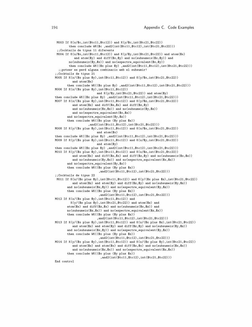
194 Appendix C. Code Examples
M003 If K(x/$c,int($tc11,$tc12)) and K(y/$c,int($tc21,$tc22))
then conclude WK($c ,and2(int($tc11,$tc12),int($tc21,$tc22)))
;;Cocktails de tipus 11 diferents
M004 If K(x/$x,int($tc11,$tc12)) and K(y/$y,int($tc21,$tc22)) and atom($x)
and atom($y) and diff($x,$y) and no(subsumeix($x,$y)) and
no(subsumeix($y,$x)) and no(espectre_equivalent($x,$y))
then conclude WK(($x plus $y) ,and2(int($tc11,$tc12),int($tc21,$tc22)))
;;potser es perd alguna combinacio amb el subsumir!
;;Cocktails de tipus 21
M005 If K(x/($x plus $y),int($tc11,$tc12)) and K(y/$x,int($tc21,$tc22))
and atom($x)
then conclude WK(($x plus $y) ,and2(int($tc11,$tc12),int($tc21,$tc22)))
M006 If K(x/($x plus $y),int($tc11,$tc12))
and K(y/$y,int($tc21,$tc22)) and atom($y)
then conclude WK(($x plus $y) ,and2(int($tc11,$tc12),int($tc21,$tc22)))
M007 If K(x/($x plus $y),int($tc11,$tc12)) and K(y/$z,int($tc21,$tc22))
and atom($z) and diff($z,$x) and diff($z,$y)
and no(subsumeix($x,$z)) and no(subsumeix($y,$z))
and no(espectre_equivalent($x,$z))
and no(espectre_equivalent($y,$z))
then conclude WK(($x plus ($y plus $z))
,and2(int($tc11,$tc12),int($tc21,$tc22)))
M008 If K(y/($x plus $y),int($tc11,$tc12)) and K(x/$x,int($tc21,$tc22))
and atom($x)
then conclude WK(($x plus $y) ,and2(int($tc11,$tc12),int($tc21,$tc22)))
M009 If K(y/($x plus $y),int($tc11,$tc12)) and K(x/$y,int($tc21,$tc22))
and atom($y)
then conclude WK(($x plus $y) ,and2(int($tc11,$tc12),int($tc21,$tc22)))
M010 If K(y/($x plus $y),int($tc11,$tc12)) and K(x/$z,int($tc21,$tc22))
and atom($z) and diff($z,$x) and diff($z,$y) and no(subsumeix($x,$z))
and no(subsumeix($y,$z)) and no(espectre_equivalent($x,$z))
and no(espectre_equivalent($y,$z))
then conclude WK(($x plus ($y plus $z))
,and2(int($tc11,$tc12),int($tc21,$tc22)))
;;Cocktails de tipus 22
M011 If K(x/($x plus $y),int($tc11,$tc12)) and K(y/($x plus $z),int($tc21,$tc22))
and atom($z) and atom($y) and diff($z,$y) and no(subsumeix($y,$z))
and no(subsumeix($z,$y)) and no(espectre_equivalent($y,$z))
then conclude WK(($x plus ($y plus $z))
,and2(int($tc11,$tc12),int($tc21,$tc22)))
M012 If K(x/($x plus $y),int($tc11,$tc12)) and
K(y/($z plus $y),int($tc21,$tc22)) and atom($z) and
atom($x) and diff($z,$x) and no(subsumeix($x,$z)) and
no(subsumeix($z,$x)) and no(espectre_equivalent($z,$x))
then conclude WK(($x plus ($y plus $z))
,and2(int($tc11,$tc12),int($tc21,$tc22)))
M013 If K(y/($x plus $y),int($tc11,$tc12)) and K(x/($x plus $z),int($tc21,$tc22))
and atom($z) and atom($y) and diff($z,$y) and no(subsumeix($y,$z))
and no(subsumeix($z,$y)) and no(espectre_equivalent($y,$z))
then conclude WK(($x plus ($y plus $z))
,and2(int($tc11,$tc12),int($tc21,$tc22)))
M014 If K(y/($x plus $y),int($tc11,$tc12)) and K(x/($z plus $y),int($tc21,$tc22))
and atom($z) and atom($x) and diff($z,$x) and no(subsumeix($x,$z))
and no(subsumeix($z,$x)) and no(espectre_equivalent($z,$x))
then conclude WK(($x plus ($y plus $z))
,and2(int($tc11,$tc12),int($tc21,$tc22)))
End control
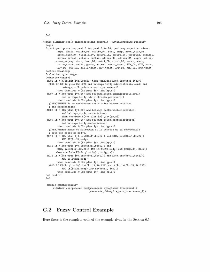
C.2. Fuzzy Control Example 195
End
Module eliminar_com(x:antimicrobians_general) : antimicrobians_general=
Begin
Export peni_procaina, peni_G_Na, peni_G_Na_DA, peni_amp_espectre, cloxa,
ampi, amoxi, eritro_DB, eritro_DA, roxi, imip, amoxi_clav_DB,
amoxi_clav_DA, ticar_clav, cefuro_OR, cefuro_EV, ceftriax, cefazol,
cefra, cefmet, cefoxi, ceftaz, clinda_DB, clinda_DA, cipro, oflox,
tetras_ac_rap, doxi, doxi_DI, cotri_DB, cotri_DI, vanco_tract,
teico_tract, amika, genta, aztreo, metro_tract, RFM_DA, GCV_tract,
ACV_DB, ACV_DA, ARA_A_tract, RBV_tract, AMD_DB, AMD_DA, RMD_tract
Control knowledge
Evaluation type: eager
Deductive control:
M001 If K(x/$x,int($tc1,$tc2)) then conclude K($x,int($tc1,$tc2))
M006 If K(($x plus $y),$V) and belongs_to($y,administracio_oral) and
belongs_to($x,administracio_parenteral)
then conclude K(($x plus $y) ,int(gp,s))
M007 If K(($x plus $y),$V) and belongs_to($x,administracio_oral)
and belongs_to($y,administracio_parenteral)
then conclude K(($x plus $y) ,int(gp,s))
;;IMPROVEMENT No es combinaran antibiotics bacteriostatics
;; amb bactericides
M008 If K(($x plus $y),$V) and belongs_to($y,bacteriostatics)
and belongs_to($x,bactericides)
then conclude K(($x plus $y) ,int(gp,s))
M009 If K(($x plus $y),$V) and belongs_to($x,bacteriostatics)
and belongs_to($y,bactericides)
then conclude K(($x plus $y) ,int(gp,s))
;;IMPROVEMENT Nomes es matxequen si la certesa de la monoterapia
;; esta per sobre de mod-p.
M010 If K(($x plus $y),int($tc11,$tc12)) and K($y,int($tc21,$tc22))
AND GT($tc21,modp)
then conclude K(($x plus $y) ,int(gp,s))
M011 If K(($x plus $y),int($tc11,$tc12)) and
K($y,int($tc21,$tc22)) AND LE($tc21,modp) AND LE($tc11, $tc21)
then conclude K(($x plus $y) ,int(gp,s))
M012 If K(($x plus $y),int($tc11,$tc12)) and K($x,int($tc21,$tc22))
AND GT($tc21,modp)
then conclude K(($x plus $y) ,int(gp,s))
M013 If K(($x plus $y),int($tc11,$tc12)) and K($x,int($tc21,$tc22))
AND LE($tc21,modp) AND LE($tc11, $tc21)
then conclude K(($x plus $y) ,int(gp,s))
End control
End
Module combmycochlam=
eliminar_com(generar_com(pneumonia_mycoplasma_tractament_2,
pneumonia_chlamydia_psit_tractament_2))
C.2 Fuzzy Control Example
Here there is the complete code of the example given in the Section 6.5.

196 Appendix C. Code Examples
C.2.1 Controller
We use four modules to implement the controller: Data, Defuzzifier, Fuzzy Infe-rence and Fuzzifier. The module Data imports the data of the problem relativeto the fuzzifier (slope and width) and the physical measures of the system (thelevel in the second tank and its variation). The module Defuzzifier exports thequantitative value of the control.
Module Data =
Begin
Import s, w, reference, h2b, deltah2b
Export s, w, reference, h2b, deltah2b
Deductive knowledge
Dictionary:
Predicates:
s = Name: "Slope"
Question: "Slope?"
Type: Numeric
w = Name: "Width"
Question: "Width?"
Type: Numeric
reference = Name: "Reference Level"
Question: "Reference Level?"
Type: Numeric
h2b = Name: "Level in the second tank"
Question: "Level in the second tank?"
Type: Numeric
deltah2b = Name: "Variation of the Level in the second tank"
Question: "Variation of the Level in the second tank?"
Type: Numeric
End Deductive
End
Module Defuzzifier =
Begin
Inherit Data
Inherit Fuzzy_Inference
Export v
Deductive knowledge
Dictionary:
Types:
Q_domain = (PL, PM, PS, P0, N0, NS, NM, NL)
Predicates:
v = Name: "Value"
Type: Numeric
Function:
(lambda ()
(let* ((slope (fact_value Data/s))
(terms (type Fuzzy_Inference/Var_u))
(values (mapcar
(function
(lambda (x) (list (first x)
(first (second x)))))
(fact_value Fuzzy_Inference/Var_u)))
(ling_terms (linguistic_terms))
(width (fact_value Data/w)))
(labels

C.2. Fuzzy Control Example 197
((real_value (ling_term)
(division (position ling_term ling_terms)
(- (length ling_terms) 1)))
(reflevel (term)
(* (- (+ 1 (position term terms))
(division (length terms) 2))
width))
(recursive_zones (values)
(let* ((value (first values))
(rest_values (cdr values))
(pla_value (center_A_n (second value)
(third value))))
(cond
(rest_values
(let ((next (recursive_zones rest_values))
(inter_value (center_union_A_n_A_np1
(second value)
(third value)
(third (first rest_values)))))
(list (+ (first pla_value)
(first inter_value)
(first next))
(+ (second pla_value)
(second inter_value)
(second next)))))
(t pla_value))))
(int_xmpot (pot sup inf)
(division (- (expt sup (+ pot 1)) (expt inf (+ pot 1)))
(+ pot 1)))
(int_constant (constant sup inf)
(* constant (int_xmpot 0 sup inf)))
(int_xmconstant (constant sup inf)
(* constant (int_xmpot 1 sup inf)))
(center_A_n (where A_n)
(let* ((origin (+ (- where width) slope))
(final (- where slope)))
(list (int_xmconstant A_n origin final)
(int_constant A_n origin final))))
(center_union_A_n_A_np1 (where A_n A_np1)
(let* ((X_A_n (+ where (* (- (* 2 A_n) 1) slope)))
(X_A_np1 (+ where (* (- 1 (* 2 A_np1)) slope)))
(X_A_n_A_np1 (+ where (* (- 1 (* 2 A_n)) slope)))
(X_A_np1_A_n (+ where (* (- (* 2 A_np1) 1) slope)))
(origin (- where slope))
(final (+ where slope)))
(labels ((int_down (sup inf)
(+ (* 0.5 (int_xmpot 0 sup inf))
(* (* 0.5 slope)
(- (int_xmpot 1 sup inf)
(* where (int_xmpot 0 sup inf))))))
(int_xmdown (sup inf)
(+ (* 0.5 (int_xmpot 1 sup inf))
(* (* 0.5 slope)
(- (int_xmpot 2 sup inf)
(* where (int_xmpot 1 sup inf))))))
(int_up (sup inf)
(- (* 0.5 (int_xmpot 0 sup inf))

198 Appendix C. Code Examples
(* (* 0.5 slope)
(- (int_xmpot 1 sup inf)
(* where (int_xmpot 0 sup inf))))))
(int_xmup (sup inf)
(- (* 0.5 (int_xmpot 1 sup inf))
(* (* 0.5 slope)
(- (int_xmpot 2 sup inf)
(* where (int_xmpot 1 sup inf)))))))
(cond
((and (greateq A_n 0.5)
(greateq A_np1 0.5))
(list (+ (int_xmconstant A_n origin X_A_n)
(int_xmdown X_A_n where)
(int_xmup where X_A_np1)
(int_xmconstant A_np1 X_A_np1 final))
(+ (int_constant A_n origin X_A_n)
(int_down X_A_n where)
(int_up where X_A_np1)
(int_constant A_np1 X_A_np1 final))))
((and (greateq A_n A_np1)
(lesseq A_np1 0.5))
(list (+ (int_xmconstant A_n origin X_A_n)
(int_xmdown X_A_n X_A_np1_A_n)
(int_xmconstant A_np1 X_A_np1_A_n final))
(+ (int_constant A_n origin X_A_n)
(int_down X_A_n X_A_np1_A_n)
(int_constant A_np1 X_A_np1_A_n final))))
((and (lesseq A_n 0.5)
(greateq A_np1 A_n))
(list (+ (int_xmconstant A_n origin X_A_n_A_np1)
(int_xmup X_A_n_A_np1 X_A_np1)
(int_xmconstant A_np1 X_A_np1 final))
(+ (int_constant A_n origin X_A_n_A_np1)
(int_up X_A_n_A_np1 X_A_np1)
(int_constant A_np1 X_A_np1 final)))))))))
(let ((result
(recursive_zones
(mapcar
(function
(lambda (term)
(list term (reflevel term)
(let ((exists
(position term
(mapcar
(function first)
values))))
(cond
(exists
(real_value (second
(nth exists values))))
(t 0))))))
terms))))
(division (first result) (second result))))))
End deductive
Control Knowledge
Evaluation type: eager
End control

C.2. Fuzzy Control Example 199
End
Module Fuzzy_Inference =
Begin
Module F = Fuzzifier
Export Var_u
Deductive knowledge
Dictionary:
Types:
Q_domain = (PL, PM, PS, P0, N0, NS, NM, NL)
Predicates:
Var_u = Name: "Qualitative ACtion"
Type: Q_domain
Rules:
R001 IF F/e int (NL) and F/Var_e int (NL) THEN conclude Var_u = (PL) is s
R002 IF F/e int (NL) and F/Var_e int (NM) THEN conclude Var_u = (PL) is s
R003 IF F/e int (NL) and F/Var_e int (NS) THEN conclude Var_u = (PL) is s
R004 IF F/e int (NL) and F/Var_e int (N0) THEN conclude Var_u = (PL) is s
R005 IF F/e int (NL) and F/Var_e int (P0) THEN conclude Var_u = (PL) is s
R006 IF F/e int (NL) and F/Var_e int (PS) THEN conclude Var_u = (PL) is s
R007 IF F/e int (NL) and F/Var_e int (PM) THEN conclude Var_u = (P0) is s
R008 IF F/e int (NL) and F/Var_e int (PL) THEN conclude Var_u = (P0) is s
R009 IF F/e int (NM) and F/Var_e int (NL) THEN conclude Var_u = (PL) is s
R010 IF F/e int (NM) and F/Var_e int (NM) THEN conclude Var_u = (PL) is s
R011 IF F/e int (NM) and F/Var_e int (NS) THEN conclude Var_u = (PM) is s
R012 IF F/e int (NM) and F/Var_e int (N0) THEN conclude Var_u = (PM) is s
R013 IF F/e int (NM) and F/Var_e int (P0) THEN conclude Var_u = (PM) is s
R014 IF F/e int (NM) and F/Var_e int (PS) THEN conclude Var_u = (PS) is s
R015 IF F/e int (NM) and F/Var_e int (PM) THEN conclude Var_u = (P0) is s
R016 IF F/e int (NM) and F/Var_e int (PL) THEN conclude Var_u = (P0) is s
R017 IF F/e int (NS) and F/Var_e int (NL) THEN conclude Var_u = (PL) is s
R018 IF F/e int (NS) and F/Var_e int (NM) THEN conclude Var_u = (PM) is s
R019 IF F/e int (NS) and F/Var_e int (NS) THEN conclude Var_u = (PS) is s
R020 IF F/e int (NS) and F/Var_e int (N0) THEN conclude Var_u = (PS) is s
R021 IF F/e int (NS) and F/Var_e int (P0) THEN conclude Var_u = (PS) is s
R022 IF F/e int (NS) and F/Var_e int (PS) THEN conclude Var_u = (P0) is s
R023 IF F/e int (NS) and F/Var_e int (PM) THEN conclude Var_u = (NS) is s
R024 IF F/e int (NS) and F/Var_e int (PL) THEN conclude Var_u = (NS) is s
R025 IF F/e int (N0) and F/Var_e int (NL) THEN conclude Var_u = (PM) is s
R026 IF F/e int (N0) and F/Var_e int (NM) THEN conclude Var_u = (PM) is s
R027 IF F/e int (N0) and F/Var_e int (NS) THEN conclude Var_u = (PS) is s
R028 IF F/e int (N0) and F/Var_e int (N0) THEN conclude Var_u = (P0) is s
R029 IF F/e int (N0) and F/Var_e int (P0) THEN conclude Var_u = (N0) is s
R030 IF F/e int (N0) and F/Var_e int (PS) THEN conclude Var_u = (NS) is s
R031 IF F/e int (N0) and F/Var_e int (PM) THEN conclude Var_u = (NM) is s
R032 IF F/e int (N0) and F/Var_e int (PL) THEN conclude Var_u = (NM) is s
R033 IF F/e int (P0) and F/Var_e int (NL) THEN conclude Var_u = (PM) is s
R034 IF F/e int (P0) and F/Var_e int (NM) THEN conclude Var_u = (PM) is s
R035 IF F/e int (P0) and F/Var_e int (NS) THEN conclude Var_u = (PS) is s
R036 IF F/e int (P0) and F/Var_e int (N0) THEN conclude Var_u = (P0) is s
R037 IF F/e int (P0) and F/Var_e int (P0) THEN conclude Var_u = (N0) is s
R038 IF F/e int (P0) and F/Var_e int (PS) THEN conclude Var_u = (NS) is s
R039 IF F/e int (P0) and F/Var_e int (PM) THEN conclude Var_u = (NM) is s
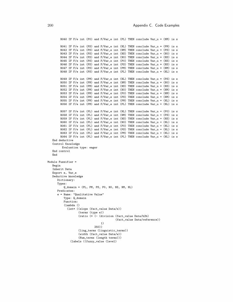
200 Appendix C. Code Examples
R040 IF F/e int (P0) and F/Var_e int (PL) THEN conclude Var_u = (NM) is s
R041 IF F/e int (PS) and F/Var_e int (NL) THEN conclude Var_u = (PM) is s
R042 IF F/e int (PS) and F/Var_e int (NM) THEN conclude Var_u = (PS) is s
R043 IF F/e int (PS) and F/Var_e int (NS) THEN conclude Var_u = (N0) is s
R044 IF F/e int (PS) and F/Var_e int (N0) THEN conclude Var_u = (NS) is s
R045 IF F/e int (PS) and F/Var_e int (P0) THEN conclude Var_u = (NS) is s
R046 IF F/e int (PS) and F/Var_e int (PS) THEN conclude Var_u = (NS) is s
R047 IF F/e int (PS) and F/Var_e int (PM) THEN conclude Var_u = (NM) is s
R048 IF F/e int (PS) and F/Var_e int (PL) THEN conclude Var_u = (NL) is s
R049 IF F/e int (PM) and F/Var_e int (NL) THEN conclude Var_u = (PS) is s
R050 IF F/e int (PM) and F/Var_e int (NM) THEN conclude Var_u = (N0) is s
R051 IF F/e int (PM) and F/Var_e int (NS) THEN conclude Var_u = (NS) is s
R052 IF F/e int (PM) and F/Var_e int (N0) THEN conclude Var_u = (NM) is s
R053 IF F/e int (PM) and F/Var_e int (P0) THEN conclude Var_u = (NM) is s
R054 IF F/e int (PM) and F/Var_e int (PS) THEN conclude Var_u = (NM) is s
R055 IF F/e int (PM) and F/Var_e int (PM) THEN conclude Var_u = (NL) is s
R056 IF F/e int (PM) and F/Var_e int (PL) THEN conclude Var_u = (NL) is s
R057 IF F/e int (PL) and F/Var_e int (NL) THEN conclude Var_u = (P0) is s
R058 IF F/e int (PL) and F/Var_e int (NM) THEN conclude Var_u = (PS) is s
R059 IF F/e int (PL) and F/Var_e int (NS) THEN conclude Var_u = (NS) is s
R060 IF F/e int (PL) and F/Var_e int (N0) THEN conclude Var_u = (NL) is s
R061 IF F/e int (PL) and F/Var_e int (P0) THEN conclude Var_u = (NL) is s
R062 IF F/e int (PL) and F/Var_e int (PS) THEN conclude Var_u = (NL) is s
R063 IF F/e int (PL) and F/Var_e int (PM) THEN conclude Var_u = (NL) is s
R064 IF F/e int (PL) and F/Var_e int (PL) THEN conclude Var_u = (NL) is s
End deductive
Control Knowledge
Evaluation type: eager
End control
End
Module Fuzzifier =
Begin
Inherit Data
Export e, Var_e
Deductive knowledge
Dictionary:
Types:
Q_domain = (PL, PM, PS, P0, N0, NS, NM, NL)
Predicates:
e = Name: "Qualitative Value"
Type: Q_domain
Function:
(lambda ()
(let* ((slope (fact_value Data/s))
(terms (type e))
(ratio (* (- (division (fact_value Data/h2b)
(fact_value Data/reference))
1)
250))
(ling_terms (linguistic_terms))
(width (fact_value Data/w))
(Num_terms (length terms)))
(labels ((fuzzy_value (level)

C.2. Fuzzy Control Example 201
(nth (truncate
(* (length ling_terms)
(division (- ratio (- level slope))
(* 2 slope))))
ling_terms))
(duplicate (x)
(list x x)))
(dolist (term terms)
(let ((reflevel
(* (- (+ 1 (position term terms))
(division Num_terms 2))
width)))
(cond ((or (eq (car (last terms)) term)
(lessthan ratio (- reflevel slope)))
(return
(list (list term
(car (last ling_terms))))))
((lessthan ratio (+ reflevel slope))
(return
(list
(list
term
(duplicate
(nth (-
(- (length ling_terms)
(position (fuzzy_value reflevel)
ling_terms)) 1)
ling_terms)))
(list
(nth (+ 1 (position term terms)) terms)
(duplicate (fuzzy_value reflevel))))))))))))
Var_e = Name: "Qualitative Value"
Type: Q_domain
Function:
(lambda ()
(let* ((slope (fact_value Data/s))
(terms (type e))
(ratio (fact_value Data/deltah2b))
(ling_terms (linguistic_terms))
(width (fact_value Data/w))
(Num_terms (length terms)))
(labels ((fuzzy_value (level)
(nth (truncate
(* (length ling_terms)
(division (- ratio (- level slope))
(* 2 slope))))
ling_terms))
(duplicate (x)
(list x x)))
(dolist (term terms)
(let ((reflevel
(* (- (+ 1 (position term terms))
(division Num_terms 2))
width)))
(cond ((or (eq (car (last terms)) term)
(lessthan ratio (- reflevel slope)))
(return

202 Appendix C. Code Examples
(list (list term
(car (last ling_terms))))))
((lessthan ratio (+ reflevel slope))
(return
(list
(list
term
(duplicate
(nth (-
(- (length ling_terms)
(position (fuzzy_value reflevel)
ling_terms)) 1)
ling_terms)))
(list
(nth (+ 1 (position term terms)) terms)
(duplicate (fuzzy_value reflevel))))))))))))
End deductive
Control Knowledge
Evaluation type: eager
End control
End
C.2.2 Simulator
We use the following Lisp function to implement the simulation of the process.
(defun simulator (h1a h2a S Q Ts)
(let* ((p1 (- (/ (+ 3 (sqrt 5)) (* 2 S))))
(p2 (/ (+ -3 (sqrt 5)) (* 2 S)))
(c2 (/ (- (* h2a (+ (* S p1) 2)) h1a (* Q S p1))
(* S (- p1 p2))))
(c1 (- h2a c2 Q))
(hb1 (+ (* c1 (exp (* p1 Ts))
(+ 2 (* S p1)))
(* c2 (exp (* p2 Ts))
(+ 2 (* S p2)))
(* 2 Q)))
(hb2 (+ (* c1 (exp (* p1 Ts)))
(* c2 (exp (* p2 Ts)))
Q))
(deltah2b (+ (* c1 p1 (exp (* p1 Ts)))
(* c2 p2 (exp (* p2 Ts))))))
(list hb1 hb2 deltah2b)))
C.2.3 Whole Process
The following Lisp functions implements the loop simulator–controller. In thecase we use a facility of the shell that consist in using a program with the externalmode. Using this mode the modules import facts by mean of an external functionnamed name of the module–import. The argument of this function is the fact tobe imported, and it returns the value of that fact. The facts required from outsidethe ES are exported by mean of another function named name of the module–export. Its argument is a list composed by the fact to be exported and its value.

C.2. Fuzzy Control Example 203
(defvar Simulator_h2b 0)
(defvar Simulator_deltah2b 0)
(defvar defuzzifier_v 0)
(defun data-import (fact)
(case fact
(s 2.5)
(w 5.0)
(reference 800)
(h2b Simulator_h2b)
(deltah2b Simulator_deltah2b)))
(defun defuzzifier-export (fact-value)
(setq defuzzifier_v (second fact-value)))
(defun two-coupled-tanks-process ()
(setq Simulator_h2b 0)
(setq Simulator_deltah2b 0)
(setq defuzzifier_v 0)
(let* ((h1a 0)
(h2a 0)
(action 0))
(dotimes (x 1000)
(let ((defuzzifier_v_old action))
(Execute ’defuzzifier ’v))
(setq action (+ defuzzifier_v_old defuzzifier_v))
(format t "(~S ~S ~S ~S ~S ~S)~%"
h1a h2a Simulator_deltah2b defuzzifier_v action (abs (- h2a 800)))
(let ((result (simulator
h1a
h2a
50
action
20)))
(setq h1a (first result))
(setq h2a (second result))
(setq Simulator_h2b (second result))
(setq Simulator_deltah2b (third result))
(ResetKB))))))
Notice that the function Execute queries the module defuzzifier for the valueof the fact v, and the function ResetKB return the ES to its original state.
Example of output:
(0 0 0 16.674 16.674 800)
(5.618 0.917 0.075 16.674 33.348 799.082)
(15.478 3.559 0.167 16.674 50.022 796.440)
(28.777 8.012 0.255 16.674 66.696 791.987)
(44.955 14.134 0.333 16.674 83.371 785.865)
(63.579 21.729 0.402 16.674 100.045 778.270)
(84.295 30.603 0.461 16.674 116.719 769.396)
(106.801 40.580 0.512 16.674 133.393 759.419)
(130.845 51.504 0.556 16.674 150.067 748.495)

204 Appendix C. Code Examples
C.3 Polytrees Example
This is the complete code of the belief propagation in bayesian polytrees givenin Section 6.6
Module POLYTREE =
Begin
Export A, B, C, D, E, F, G
Deductive knowledge
Dictionary:
Types:
dom_A = (a0 or a1)
dom_B = (b0 or b1 or b2)
dom_C = (c0 or c1 or c2)
dom_D = (d0 or d1)
dom_E = (e0 or e1)
dom_F = (f0 or f1 or f2)
dom_G = (g0 or g1 or g2)
Predicates:
A =
Name: "A"
Type: array [dom_A]
A_prior =
Name: "P(A) Prior probability of A"
Question: "Enter P(A), prior probability for A"
Type: array [dom_A]
Relation: prior A
A_ptr =
Name: "Pointer to A"
Type: logic
Relation: points_to A
B =
Name: "B"
Type: array [dom_B]
B_prior =
Name: "P(B) Prior probability of B"
Question: "Enter P(B), prior probability for B"
Type: array [dom_B]
Relation: prior B
B_ptr =
Name: "Pointer to B"
Type: logic
Relation: points_to B
C =
Name: "C"
Type: array [dom_C]
C_prior =
Name: "P(C), prior probability of C"
Question: "Enter P(C), prior probability for C"
Type: array [dom_C]
Relation: prior C
C_ptr =
Name: "Pointer to C"
Type: logic
Relation: points_to C
D =
Name: "D"

C.3. Polytrees Example 205
Type: array [dom_D]
D_ptr =
Name: "Pointer to D"
Type: logic
Relation: points_to D
E =
Name: "E"
Type: array [dom_E]
E_ptr =
Name: "Pointer to E"
Type: logic
Relation: points_to E
E_evid =
Name: "Evidence for E"
Question: "Enter evidence for E"
Type: array [dom_E]
Relation: evid E
F =
Name: "F"
Type: array [dom_F]
F_ptr =
Name: "Pointer to F"
Type: logic
Relation: points_to F
F_evid =
Name: "Evidence for F"
Question: "Enter evidence for F"
Type: array [dom_F]
Relation: evid F
G =
Name: "G"
Type: array [dom_G]
G_ptr =
Name: "Pointer to G"
Type: logic
Relation: points_to G
G_evid =
Name: "Evidence for G"
Question: "Enter evidence for G"
Type: array [dom_G]
Relation: evid G
Rules:
R01 If A_ptr and B_ptr and C_ptr then conclude D_ptr is
((((0.3 0.7) (0.4 0.6) (0.5 0.5))
((0.75 0.25) (0.82 0.18) (0.35 0.65))
((0.45 0.55) (0.8 0.2) (0.1 0.9)))
(((0.3 0.7) (0.99 0.01) (1 0))
((0.37 0.63) (0.85 0.15) (0.21 0.79))
((0.45 0.55) (0.99 0.01) (0.27 0.73))))
;; pi_jkl = p (Di / Aj Bk Cl)
;; ((((p0_000 p1_000) (p0_001 p1_001) (p0_002 p1_002))
;; ((p0_010 p1_010) (p0_011 p1_011) (p0_012 p1_012))
;; ((p0_020 p1_020) (p0_021 p1_021) (p0_022 p1_022)))
;; (((p0_100 p1_000) (p0_101 p1_001) (p0_102 p1_002))
;; ((p0_110 p1_010) (p0_111 p1_011) (p0_112 p1_012))
;; ((p0_120 p1_020) (p0_121 p1_021) (p0_122 p1_022))))

206 Appendix C. Code Examples
R02 If D_ptr and B_ptr then conclude E_ptr is ((0.75 0.25) (0.55 0.45))
R03 If D_ptr then conclude F_ptr is ((0.3 0.2 0.5) (0.1 0.5 0.4))
R04 If D_ptr then conclude G_ptr is ((0.3 0.6 0.1) (0.5 0.2 0.3))
End deductive
Control knowledge
Evaluation type: reified
Deductive control:
;; --------------------------------------------
;; Translation metarules
M01 If K(implies ($list_of_premises,$conclusion),$matrix) and
points_to ($conclusion,$child) and
set_of_instances ($father,
conj ( position ($prem,$list_of_premises,$i),
points_to ($prem,$father)),
$list_of_fathers)
then conclude
K(cause ($list_of_fathers,$child),$matrix)
M02 If points_to ($x_ptr,$x) then conclude node($x)
;; --------------------------------------------
;; Initializes nodes with evidence
M03 If evid($x_evid,$x) and K($x_evid,$v)
then conclude K(lambda ($x),$v)
;; --------------------------------------------
;; Initializes root nodes
M04 If prior($x_prior,$x) and K($x_prior,$v)
then conclude K(pi($x),$v)
;; --------------------------------------------
;; Lambda propagation
;; Calculates lambda messages for nodes with several fathers.
M05 If K(cause ($list_of_fathers,$child),$matrix) and
K(lambda ($child),$lambda_child) and
position($father_i,$list_of_fathers,$i) and
set_of_instances($msg,
conj(position($father_k,$list_of_fathers,$k),
neg(equal($k,$i)),
K(pi_msg($father_k,$child),$msg)),
$pi_msgs_fathers_minus_i)
then conclude K(lambda_msg($child,$father_i),
matrix_prod ($lambda_child,
transpose (matrix_prod%
(cartesian_prod%($pi_msgs_fathers_minus_i),
reduce_dim ($matrix, $i)))))
;; Calculates lambda messages for nodes with only one father
M06 If K(cause($list_of_fathers,$child),$matrix) and
cardinal($list_of_fathers,1) and
position ($father,$list_of_fathers,$i) and
K(lambda($child),$lambda_child)
then conclude K(lambda_msg($child,$father),
matrix_prod($lambda_child,transpose($matrix)))
;; lambda update
M07 If node($father) and
set_of_instances($msg,K(lambda_msg($child,$father),
$msg),$lambda_msgs_children)
then conclude K(lambda($father),

C.3. Polytrees Example 207
inner_product($lambda_msgs_children))
;; --------------------------------------------
;; Pi propagation
;; Calculates pi messages for nodes with several children
M08 If K(cause($list_of_fathers,$child_j),$matrix) and
position($father,$list_of_fathers,$i) and
K(pi($father),$pi_father) and
set_of_instances($msg,
conj(K(lambda_msg($child_k,$father),$msg),
neg (equal($child_k,$child_j))),
$lambda_msgs_children_minus_j)
then conclude K(pi_msg($father,$child_j),
norm (inner_product
(inner_product ($lambda_msgs_children_minus_j),
$pi_father)))
;; Calculates pi messages for nodes with a unique child
M09 If K(cause($list_of_fathers,$child),$matrix) and
position($father,$list_of_fathers,$i) and
K(pi($father),$pi_father) and
no(set_of_instances ($child_j,
conj(K(lambda_msg($child_j,$father),$msg),
neg(equal($child_j,$child))),
$other_children))
then conclude K(pi_msg($father,$child),$pi_father)
;; Pi update
M10 If K(cause($list_of_fathers,$child),$matrix) and
set_of_instances ($msg,
conj(position($father_i,$list_of_fathers,$i),
K(pi_msg($father_i,$child),$msg)),
$pi_msgs_fathers)
then conclude K(pi($child),
norm(matrix_prod
(cartesian_prod% ($pi_msgs_fathers),
$matrix)))
;; --------------------------------------------
;; Belief update
M11 If K(lambda($x),$lambda_x) and
K(pi($x),$pi_x)
then conclude K($x,norm(inner_product($lambda_x,$pi_x)))
End control
End

208 Appendix C. Code Examples

List of Figures
2.1 Example of module declaration. . . . . . . . . . . . . . . . . . . . 212.2 Syntax of interfaces. . . . . . . . . . . . . . . . . . . . . . . . . . 222.3 Example of module declaration. . . . . . . . . . . . . . . . . . . . 232.4 Syntax of modules. . . . . . . . . . . . . . . . . . . . . . . . . . . 242.5 Hierarchy example. . . . . . . . . . . . . . . . . . . . . . . . . . . 272.6 Example of generic module definition and application. . . . . . . 302.7 Syntax of generic modules. . . . . . . . . . . . . . . . . . . . . . 312.8 Example of module used as parameter of a generic module. . . . 312.9 Kernel declaration scheme. . . . . . . . . . . . . . . . . . . . . . 332.10 Syntax of refinement, contraction and expansion. . . . . . . . . . 342.11 Example of generic module definition and application. . . . . . . 352.12 Example of module refinement. . . . . . . . . . . . . . . . . . . . 382.13 Example of module refinement. . . . . . . . . . . . . . . . . . . . 392.14 Visibility example (hidden modules are written in italic). . . . . 402.15 Syntax of submodule declarations. . . . . . . . . . . . . . . . . . 422.16 Example of open module. . . . . . . . . . . . . . . . . . . . . . . 422.17 Syntax of sharing. . . . . . . . . . . . . . . . . . . . . . . . . . . 43
3.1 Example of Local logic declaration. . . . . . . . . . . . . . . . . . 493.2 Fuzzy set representing the concept tall. . . . . . . . . . . . . . . . 523.3 Imprecision Ordering on Int(A4). . . . . . . . . . . . . . . . . . . 553.4 Weak Uncertainty Ordering on Int(A4). . . . . . . . . . . . . . . 563.5 Mapping example. . . . . . . . . . . . . . . . . . . . . . . . . . . 643.6 Logic declaration. . . . . . . . . . . . . . . . . . . . . . . . . . . . 653.7 Trapezoidal approximation of a fuzzy interval. . . . . . . . . . . . 663.8 Truth table declaration for TA5
. . . . . . . . . . . . . . . . . . . . 673.9 Renaming declaration example. . . . . . . . . . . . . . . . . . . . 683.10 Example of logic declaration. . . . . . . . . . . . . . . . . . . . . 69
4.1 Standard Behavior of an ES. . . . . . . . . . . . . . . . . . . . . 724.2 Inference Engine Architecture. . . . . . . . . . . . . . . . . . . . 744.3 Example of specialization of a KB . . . . . . . . . . . . . . . . . 794.4 Deductive declaration into the modules. . . . . . . . . . . . . . . 944.5 Example of dictionary declaration . . . . . . . . . . . . . . . . . 95
209

210 LIST OF FIGURES
4.6 Example of function attribute . . . . . . . . . . . . . . . . . . . . 984.7 Example of characteristic function. . . . . . . . . . . . . . . . . . 994.8 Syntax of the rules. . . . . . . . . . . . . . . . . . . . . . . . . . . 1014.9 Syntax of the conditions of rules. . . . . . . . . . . . . . . . . . . 1024.10 Syntax of the conclusion of rules. . . . . . . . . . . . . . . . . . . 104
5.1 Control declaration . . . . . . . . . . . . . . . . . . . . . . . . . . 1095.2 Example of subsumption. . . . . . . . . . . . . . . . . . . . . . . 1145.3 Control cycle. . . . . . . . . . . . . . . . . . . . . . . . . . . . . . 1205.4 Syntax of the premises of metarules. . . . . . . . . . . . . . . . . 1235.5 Syntax of the deductive control. . . . . . . . . . . . . . . . . . . . 1245.6 Syntax of the structural control. . . . . . . . . . . . . . . . . . . 125
6.1 Architecture of Terap–IA application. . . . . . . . . . . . . . . . 1296.2 Example of filtering. . . . . . . . . . . . . . . . . . . . . . . . . . 1326.3 Module Renal Failure. . . . . . . . . . . . . . . . . . . . . . . . . 1336.4 Module Pneumonia Mycoplasma Treatment. . . . . . . . . . . . . 1356.5 Example of module tree. . . . . . . . . . . . . . . . . . . . . . . . 1376.6 Case example. . . . . . . . . . . . . . . . . . . . . . . . . . . . . . 1386.7 Coupled tanks example. . . . . . . . . . . . . . . . . . . . . . . . 1396.8 Scheme of the process. . . . . . . . . . . . . . . . . . . . . . . . . 1406.9 Fuzzy control modules. . . . . . . . . . . . . . . . . . . . . . . . . 1426.10 Fuzzification process. . . . . . . . . . . . . . . . . . . . . . . . . . 1426.11 Defuzzication by mean of the gravity center. . . . . . . . . . . . . 1456.12 Results for h2, dQ and Q. . . . . . . . . . . . . . . . . . . . . . . 1466.13 Detailed dQ. . . . . . . . . . . . . . . . . . . . . . . . . . . . . . 1476.14 Phase plane result. . . . . . . . . . . . . . . . . . . . . . . . . . . 1486.15 Node example. . . . . . . . . . . . . . . . . . . . . . . . . . . . . 1486.16 Comparations among applications. . . . . . . . . . . . . . . . . . 156

List of Tables
1.1 Main differences between Milord and Milord II. . . . . . . . . . 5
3.1 TS5Table. . . . . . . . . . . . . . . . . . . . . . . . . . . . . . . . 49
3.2 N5 Table. . . . . . . . . . . . . . . . . . . . . . . . . . . . . . . . 503.3 ITS5
(x, y) Table. . . . . . . . . . . . . . . . . . . . . . . . . . . . 503.4 MPTS5
(x, y) Table. . . . . . . . . . . . . . . . . . . . . . . . . . . 513.5 TGram7
Table. . . . . . . . . . . . . . . . . . . . . . . . . . . . . . 63
4.1 Main differences between Milord and Milord II inference engines 804.2 Valid models of the example. . . . . . . . . . . . . . . . . . . . . 854.3 Operations between expressions. . . . . . . . . . . . . . . . . . . 104
6.1 Mac Vicar–Wheland’s initial set of rules. . . . . . . . . . . . . . . 144
211

212 LIST OF TABLES

References
Agustı, J., Sierra, C. and Sannella, D. (1989). Methodologies for IntelligentSystems, 4, chapter Adding generic modules to flat rule–based languages: A lowcost approach, pages 43–51. Elsevier Science Publishing Co., Inc.
Agustı, J., Esteva, J., Garcia, P., Godo, L. and Sierra, C. (1991). Combiningmultiple–valued logics in modular expert systems. In Proceedings 7th Conferenceon Uncertainty in AI.
Agustı, J., Esteva, F., Garcia, P., Godo, L., Lopez de Mantaras, R., Puyol, J.,Sierra, C. and Murgui, L. (1992). Fuzzy Logic for the Management of Uncer-tainty, chapter Structured Local Fuzzy Logics in Milord, pages 523–551. JohnWiley and Sons, Inc.
Alsina, C., Grane, J., Sales, T. and Trillas, E. (1984). Algunes consideracionssobre el modus ponens: Funcions de modus ponens. In Actes del III CongresCatala de Logica Matematica. Barcelona, pages 55–77.
Arcos, J. L. (1992). Definicio i implementacio d’un compilador per a Milord II.Master’s thesis, Universitat Politecnica de Catalunya, Barcelona.
Barroso, C. (1992). ENS–AI: un sistema experto para la ensenanza. In Proceed-ings of the European Conference about Information Technology in Education: acritical insight. Barcelona., volume 2, pages 373–382.
Belmonte, M. (1991). Renoir: Un sistema experto para la ayuda en el diagnosticode colagenosis y artropatias inflamatorias. PhD thesis, Universitat Autonomade Barcelona.
Berenji, H. R. (1992). An Introduction to Fuzzy Logic Applications in Intelli-gent Systems, chapter Fuzzy Logic Controllers, pages 69–96. Kluwer AcademicPublishers.
Bonissone, P., Gans, S. and Decker, K. (1987). Rum: A layered architecture forreasoning with uncertaintyg. In IJCAI’87, pages 891–898.
Chandrasekaran, B. (1986). Generic tasks in knowledge–based reasoning: High–level building blocks for expert systems design. Technical report, Ohio StateUniversity.
213

214 REFERENCES
Chandrasekaran, B. (1987). Towards a functional architecture for intelligencebased on generic information processing tasks. In Proceedings of the IJCAI’87,pages 1183–1192.
Davis, R. (1982). Knowledge–Based Systems in Artificial Intelligence, chapterTEIRESIAS: Applications of Meta–Level Knowledge, pages 920–927. McGraw–Hill, New York.
Dechter, R., Meiri, I. and Pearl, J. (1991). Temporal constraint networks. Arti-ficial Intelligence, 49:61–95.
Demolombe, R. (1990). Strategies for the computation of conditional answers.In Proceedings of the Workshop on Partial Deduction, Partial Evaluation andIntelligent Reasoning, ECAI’90, pages 5–23.
Dempster, A. P. (1967). Upper and lower probabilities induced by a multivaluedmapping. Annals of Mathematical Statistics, 38:325–339.
Domingo, M. (1993a). Evaluating the expert system approach to biologicalidentification through application to porifera. In Sponges in Time and Space.Proceedings 4th International Porifera Congress, page In press.
Domingo, M. (1993b). Towards a knowledge level analysis of classification inbiological domains. In Proceedings of the IMACS International Workshop onQualitative Reasoning and Decision Technologies QUARDET’93., pages 535–544.
Domingo, M. (1995). An expert system architecture for taxonomic domains. Anapplication in Porifera: the development of Spongia. PhD thesis, Universitat deBarcelona.
Dubois, D. and Prade, H. (1988). Possibility Theory: An Approach to Comput-erized Processing of Uncertainty. Plenum Press.
Duda, R. O., Hart, P. E. and Nilsson, N. J. (1976). Subjective bayesian meth-ods for rule–based inference systems. In Proceedings of the AFIPS NationalComputer Conference, volume 7, pages 1075–1082.
Esteva, F., Garcia-Calves, P. and Godo, L. (1994). Enriched interval bilattices:An approach to deal with uncertainty and imprecision. Uncertainty, Fuzzynessand Knowledge–Based Systems (to appear).
Fensen, D., Angele, J. and Landes, D. (1991). Karl: A knowledge adquisitionand representation language. In Proceedings of the 11th Conference on ExpertSystems and their Applications (Avignon), pages 513–525.
Forgy, C. (1981). OPS5 user manual. Technical Report CMU–CS–81–135, Com-puter Science Department, Carnegie Melon University.

REFERENCES 215
Foulloy, L. (1993). Qualitative control and fuzzy control: Towards a writingmethodology. AICOM, 6(3/4).
Fox, J. (1989). Knowledge Engeneering, chapter Symbolic Decision Proceduresfor Knowledge Based Systems. McGraw Hill.
Gallagher, J. (1986). Transforming logic programming by specialising inter-preters. In Proceedings ECAI’86, pages 109–122.
Giunchiglia, E., Traverso, P. and Giunchiglia, F. (1993). Formal Specification ofComplex Reasoning Systems, chapter Multi–Context Systems as a SpecificationFramework for Complex Reasoning Systems. Ellis Horwood.
Godo, L., Lopez de Mantaras, R., Sierra, C. and Verdaguer, A. (1988). Managinglinguistically expressed uncertainty in milord application to medical diagnosis.AI Communication, 1(1):14–31.
Godo, L., Lopez de Mantaras, R., Sierra, C. and Verdaguer, A. (1989). Milord:The architecture and management of linguistically expressed uncertainty. Inter-national Journal of Intelligent Systems, 4:471–501.
Godo, L. and Meseguer, P. (1991). A constraint–based approach to generatefinite truth–values algebras. Technical Report 91/9, IIIa–CEAB.
Goguen, J. A. (1986). Reusing and interconnecting software components. IEEEComputer, February:16–28.
Greboval, C. and Kassel, G. (1992). Modelling at the knowledge level: Theshell AIDE. In Proceedings of the 12th International Conference on ArtificialIntelligence, Expert Systems and Natural Language, Avignon, France.
Hajek, P., Havranek, T. and Jirousek, R. (1992). Processing Uncertain Infor-mation in Expert Systems. CRC Press.
Harper, R., McQueen, D. and Milner, R. (1986). Standard ML. Technical ReportECS–LCFS–86–2, Edinburgh University.
Harper, R., Sannella, D. and Tarlecki, A. (1989). Structure and representationin LCF. In Proceedings of 4th IEEE Symp. on Logic of Computer Science.
Jonckers, V., Geldof, S. and De Vroede, K. (1992). The COMMET methodologyand workbench in practice. Technical Report 92–8, Vrije Universiteit Brussel.Laboratory for Artificial Intelligence.
Kleene, S. (1952). Introduction to Metamathematics. Van Nostrand.
Komorowski, H. J. (1981). A specification of an abstract Prolog machine and itsapplication to partial evaluation. PhD thesis, Linkoping University.
Komorowski, H. J. (1990). Towards a programming methodology founded onpartial deduction. In Proceedings ECAI’90, pages 404–409.

216 REFERENCES
Kuipers, B., Moskowitz, A. and Kassirer, J. (1988). Critical decisions underuncertainty: Representation and structure. Cognitive Science, 12:177–210.
Langevelde, I. v., Philipsen, A. and Treur, J. (1993). Formal Specification ofComplex Reasoning Systems, chapter A Compositional Architecture for SimpleDesign Formally Specified in DESIRE. Ellis Horwood.
Lloyd, J. W. and Shepherson, J. C. (1991). Partial evaluation in logic program-ming. The Journal of Logic Programming, 11(3/4):217–242.
Lopez de Mantaras, R. (1990). Approximate Reasoning Models. Ellis HorwoodSeries in Artificial Intelligence.
Lopez, B. (1993). Aprenentatge i generacio de plans per a Sistemes Experts.PhD thesis, Universitat Politecnica de Catalunya, Barcelona.
Meseguer, P. (1992). Validation of Multi–Level Rule–Based Expert Systems. PhDthesis, Universitat Politecnica de Catalunya, Barcelona.
Miller, D. A. (1986). A theory of modules for logic programming. In AAVV:Proceedings of 1986 IEEE Sympos. on Logic Programming.
Nilsson, N. J. (1986). Probabilistic logic. Artificial Intelligence Journal, 28:71–88.
O’Keefe, R. (1985). Towards an algebra for constructing logic programs. InAAVV: Proceedings of 1985 IEEE Sympos. on Logic Programming, pages 152–160.
Pearl, J. (1986). A constrain–propagation approach to probabilistic reasoning.In Kanal, N. L. and Lemmer, J. F., editors, Uncertainty in Artificial Intelligence,pages 357–369. North Holland.
Pearl, J. (1988). Probabilistic Reasoning in Intelligent Systems: Networks ofPlausible Inference. Morgan Kaufmann.
Pearl, J. (1990). Reasoning under uncertainty. Annual Review in ComputerScience, 4:37–42.
Plaza, E. and Lopez de Mantaras, R. (1989). Model–based knowledge acquisitionfor heuristic classification systems. SIGART Newsletter, 108:98–105.
Puyol, J. (1989a). Hacia un modelo de computacion concurrente para sistemasexpertos. In Proceedings III Reunion Tecnica de la Asociacion Espanola para laInteligencia Artificial, pages 23–31.
Puyol, J. (1989b). Parallel programming in expert systems. In Proceedings ThirdWorld Conference on Mathematics at the Service of Man.
Puyol, J. (1990). ADES: un entorn per a sistemes experts distribuıts. Master’sthesis, Universitat Autonoma de Barcelona.
REFERENCES 217
Puyol, J., Sierra, C. and Agustı, J. (1991). Partial evaluation in MILORD II: Alanguage for knowledge engineering. In Proceedings Europ–IA’91, pages 193–207.
Puyol, J. (1992a). An inference engine based on specialisation with uncertainty.In Proceedings IPMU’92, pages 725–728.
Puyol, J., Godo, L. and Sierra, C. (1992b). A specialisation calculus to improveexpert system communication. In Proceedings ECAI’92, pages 144–148.
Puyol, J., Godo, L. and Sierra, C. (1992c). A specialisation calculus to improveexpert system communication (long paper). Technical Report 92/8, IIIA–CSIC.
Sakama, C. and Itoh, H. (1986). Partial evaluation of queries in deductivedatabases. Technical Report TR–302, ICOT.
Sannella, D. and Wallen, L. A. (1987). A calculus for the construction of mod-ular prolog programs. In AAVV: Proceedings of 1987 IEEE Sympos. on LogicProgramming, pages 368–378.
Shafer, G. (1976). A mathematical theory of the evidence. Princeton UniversityPress.
Shortliffe, E. H. and Buchanan, B. G. (1975). A model of inexact reasoning inmedecine. Mathematical Biosciencies, 23:351–379.
Shortliffe, E. H. (1976). Computer Based Medical Consultations: MYCIN. Amer-ican Elsevier, New York.
Sierra, C. (1989). MILORD: Arquitectura multi–nivell per a sistemes experts enclassificacio. PhD thesis, Universitat Politecnica de Catalunya, Barcelona.
Sierra, C. and Agustı, J. (1991). Colapses: Towards a methodology and a lan-guage for knowledge engineering. In Proceedings AVIGNON’91, pages 407–423.
Steele, G. (1984). Common Lisp: The Language. Digital Press.
Steels, L. (1990). Components of expertise. AI Magazine, 11.
Sticklen, J., Smith, J. W., Chandrasekaran, B. and Josephson, J. R. (1987). Mod-ularity of domain knowledge. International Journal of Expert Systems, 1(1):1–15.
Takeuchi, A. and Furukawa, K. (1986). Partial evaluation of prolog programsand its application to meta programming. In Information Processing 86.
Treur, J. and Wetter, T., editors (1993). Formal Specification of Complex Rea-soning Systems. Ellis Horwood.
Trillas, E. and Valverde, L. (1987). On inference in fuzzy logic. In Second IFSACongress. Tokyo, pages 294–297.
Turner, R. (1984). Logics for Artificial Intelligence. Ellis Horwood Series inArtificial Intelligence.

218 REFERENCES
Valverde, L. and Trillas, E. (1985). On modus ponens in fuzzy logic. In Pro-ceedings 15th ISMVL. Kignston (Ontario), pages 294–301.
van Harmelen, F. and Balder, J. (1992). (ML)2: A formal language for KADSmodels of expertise. Knowledge Acquisition, 4(1).
van Harmelen, F., Lopez de Mantaras, R. and Malec, J. (1993). Formal Specifi-cation of Complex Reasoning Systems, chapter Comparing Formal SpecificationLanguages for Complex Reasoning Systems, pages 257–282. Ellis Horwood.
Vasey, P. (1986). Qualified answers and their application to transformation. InGoos, G. and Hartmanis, J., editors, Third International Conference in LogicProgramming, LNCS 225, pages 425–432. Springer–Verlag.
Veld, L., Jonker, W. and Spee, J. (1993). Formal Specification of Complex Rea-soning Systems, chapter Specifications of Complex Reasoning Tasks in KBSSF .Ellis Horwood.
Venken, R. (1984). A prolog meta–interpreter for partial evaluation and itsapplication to source transformation and query–optimisation. In ProceedingsECAI’84, pages 91–100.
Verdaguer, A. (1989). Pneumon–IA: Desenvolupament i validacio d’un sis-tema expert d’ajuda al diagnostic medic. PhD thesis, Universitat Autonomade Barcelona.
Vicar-Whelan, P. J. M. (1976). Fuzzy sets for man–machine interaction. Inter-national Journal of Man–Machine Studies, 84:687–697.
Vila, L. (1993a). Constraints on distances between temporal distances. Reportde Recerca forthcoming, IIIA.
Vila, L. (1993b). Instants, periods and the divided instant problem. In proc. ofQUARDET’93. IMACS.
Vila, L. (1993c). A theory of time based on instants and periods. Report deRecerca forthcoming, IIIA. Submitted to 1rst Intl. Conf. on Temporal Logic.
Vila, L. (1993d). Time ontology and temporal occurrence predicates. In TAR-RAT’93. IIIA.
Vila, L. (1995). On Temporal Representation and Reasoning in Knowledge–BasedSystems. PhD thesis, Universitat Politecnica de Catalunya, Barcelona.
Wielinga, B. J., Schreiber, A. T. and Breuker, J. A. (1992). Kads: A modellingapproach to knowledge engineering (special issue). Knowledge Acquisition, 4(1).
Wolstenholme, D. (1987). Saying i don’t know and conditional answers. InMoralle, D., editor, Research and Development in Expert Systems IV, pages115–125. Cambridge University Press.

REFERENCES 219
Zadeh, L. A. (1965). Fuzzy sets. Inf. Control, 8:338–353.
Zadeh, L. A. (1975). Fuzzy logic and approximate reasoning. Synthese, 30:407–428.

220 REFERENCES

Index
Ens–AI, 136Milord, 3Spong–IA, 136Terap–IA, 128, 177
Algebra of truth–values, 47
Completeness, 87, 171Contraction, 32, 40
Deductive Control, 124Deductive Knowledge, 94Deductive Process, 74Dynamic Modules, 43
Eager, 119, 125Evaluation Strategy, 117Expansion, 32, 40
Fact Declarations, 95Fact Types, 96Fuzzy Control Example, 139, 195Fuzzy Sets, 57, 98
Generic Modules, 19, 28
Hierarchy of modules, 24
Imprecision, 45, 53Inference Engine, 88Information Hiding, 37Inherit Declaration, 41Inheritance, 36Interfaces, 22Intervals of Truth–values, 54
Lazy, 117, 125Local Logic Declaration, 65
Local Logics, 60
Metarules, 124Modules, 18, 25
Open Declaration, 41
Propagation Rules Example, 146, 204
Refinement, 32, 34Reflection, 119Reification, 119Reified, 125Rule Declarations, 100
Search Process, 73Search Strategy, 117Semantics of Specialization, 82Sharing Declaration, 43Soundness, 87, 171Specialization, 9, 76, 90Specialization Calculus, 81Structural Control, 124Subsumption, 109Syntax of Milord II, 161Syntax of Specialization, 81
Threshold, 116
Uncertainty, 45, 51Unnecessary Rules, 115
Validation, 79
221