monopolistic competition - econ.msu.ru
TRANSCRIPT

Unit 8. Firm behaviour
and market structure:
monopolistic competition
and oligopoly
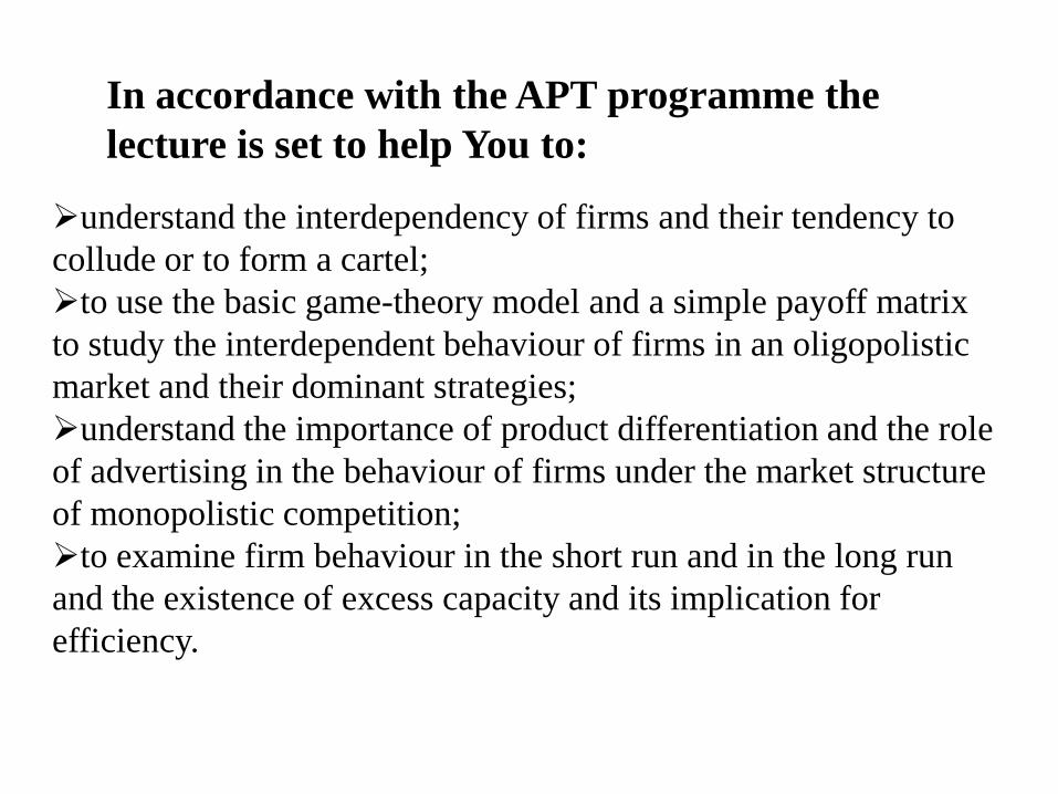
In accordance with the APT programme the
lecture is set to help You to:
understand the interdependency of firms and their tendency to
collude or to form a cartel;
to use the basic game-theory model and a simple payoff matrix
to study the interdependent behaviour of firms in an oligopolistic
market and their dominant strategies;
understand the importance of product differentiation and the role
of advertising in the behaviour of firms under the market structure
of monopolistic competition;
to examine firm behaviour in the short run and in the long run
and the existence of excess capacity and its implication for
efficiency.

Required reading Begg, D., R.Dornbusch, S.Fischer. Economics. 8th
edition. McGraw Hill. 2005.
Chapter 9. Market structure and imperfect competition:
9.2. Monopolistic competition
9.3. Oligopoly and interdependence
9.4. Game theory and interdependent decisions
9.5. Reaction functions
9.6. Entry and potential competition
9.7. Strategic entry deterrence
9.8. Summing up.

Questions to be revised
The relationships among the short-run and long-run
costs: total, average and marginal;
The profit-maximizing rule;
Profit maximization by a competitive firm in the
short run and in the long run;
Production and allocation efficiency.

Perfect
Competition
Imperfect Competition
Monopolistic
Competition
Monopoly and
Oligopoly
Many buyers and
sellers
Many buyers and
sellers
One or few sellers
(large)
Firms are too small
to affect price
Can affect price Can affect price
Identical
(homogeneous)
products
Goods are close
substitutes
Homogeneous or
heterogeneous
goods
Free entry and exit Free entry and exit Big entry costs
Zero profits in the
long run
Zero profits in the
long run
Profits can be
positive

Monopolistic Competition and Oligopoly
• Monopolistic competition: many sellers produce products that are close (but not perfect!) substitutes for one another. Example: beer market.
• Oligopoly: few producers, each recognizes that its own price depends on the actions of other firms in the industry. Example: aircraft manufacturing (Boeing and Airbus).

Monopolistic Competition
• Lots of small firms
• Downward-sloping demand curve
• Product differentiation (brand, location)
• Free entry
• Zero profits in the long run

Long run equilibrium of a firm under
monopolistic competition
Short run equilibrium of a firm under
monopolistic competition: economic profits
Free entry of new firms to the
market with positive economic
profits shifts residual demand
of a monopolistic competitor
until:
Q*
MR D
MR
D
Q*
P*
PR
P, MR,
MC, AC
AC
0
MC
Q
P*
QK
PK P=AC
MR=MC
First order condition:
Excess capacity: QK‒Q* Cost of product diversity:
P*‒PK

Monopolistic Competition in the LR
Note:
1. Firms are not producing at lowest point of AC curve;
2. Price exceeds MC.

Example: APT 2007 (Form B)
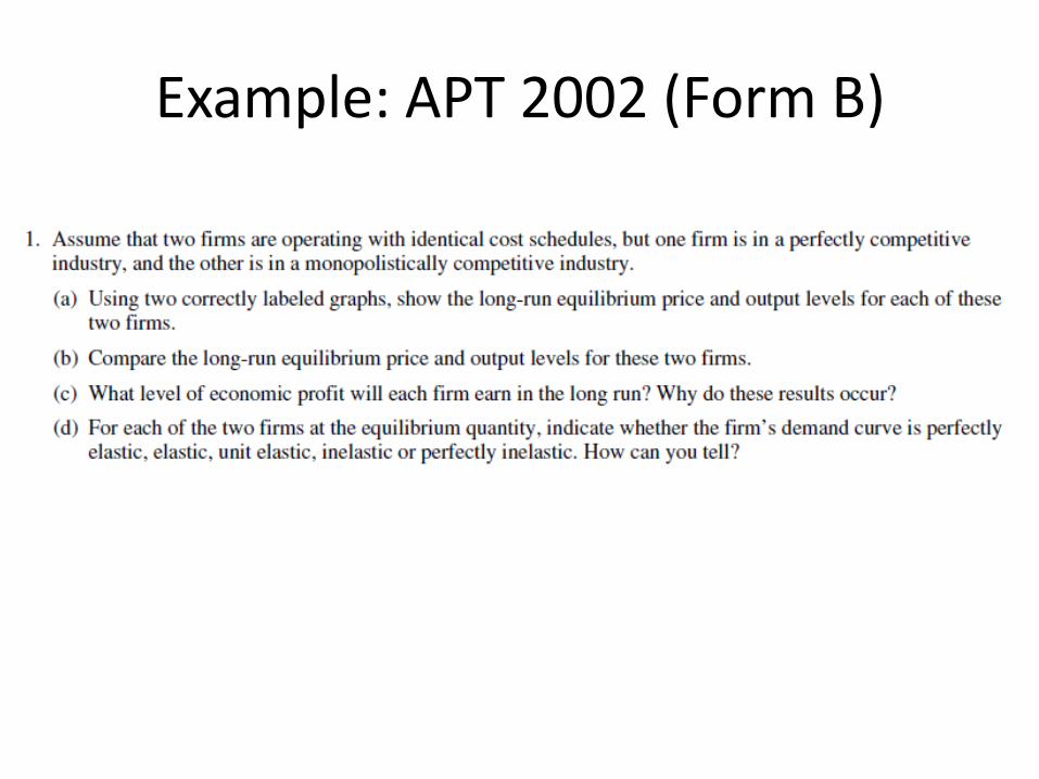
Example: APT 2002 (Form B)

Profit maximization by a monopolistic
competitor in long run
0
d Qp d Q ACdPR dTR dTC dP dACP Q AC Q
dQ dQ dQ dQ dQ dQ dQ
dP dACP Q AC Q
dQ dQ
dP dAC
dQ dQ
P=AC
First order condition:
It follows that:
Apply zero profit condition
to get
Consequently, average cost and residual demand curves
for a monopolistic competitor are tangent in long run.

Long run equilibrium of a firm under
monopolistic competition
Short run equilibrium of a firm under
monopolistic competition: economic losses
Free exit from the market of
firms which meet a loss shifts
residual demand of a
monopolistic competitor upwards
until:
Q*
MR
D MR
D
Q*
P*
Loss
P, MR,
MC, AC
AC
0
MC
Q
P*
QK
PK
P=AC
MR=MC
First order condition:
Excess capacity: QK‒Q* Cost of product diversity:
P*‒PK
AVC
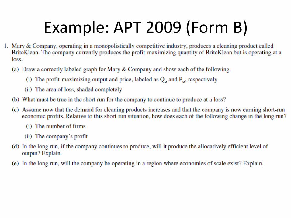
Example: APT 2009 (Form B)

Interdependent Decisions
Monopolistic competition – each firm is too small and there are too many firms. Assume decisions of firms are not interdependent.
Oligopoly – few large firms. Need for strategic behaviour. Need for each firm to consider how its own decisions affect the decisions of its competitors.

Game Theory
Analysis of interdependent decisions: actions of one decision maker affect payoffs of another decision maker.
Three elements of any game:
- Players (participants);
- List of possible actions (strategies);
- Payoffs of players (depend on player’s own actions AND actions of other players); measured as utilities/profits.

Game models of oligopoly
can be classified according to: • Number of players (classical optimization is a single player
game)
• Number of strategies: finite or infinite
• Properties of payoff functions: zero sum (antagonistic),
nonzero sum, constant difference (surpluses and losses at the
same time)
• Possibility of pre-game negotiations and interaction during
the game (cooperative or noncooperative)
• Temporal profile of decision making (simultaneous move or
sequential moves)
• Number of interactions (single move or repeated games)

Games with simultaneous moves
Each player makes a decision independently (not knowing what the other decides), and then the payoffs are realized.
Players have complete information or common knowledge of all factors of the game.
Payoff matrix – a table that describes the payoffs in a game for each possible combination of strategies.

Nash equilibrium is a set of strategies such that no player has an incentive to deviate from his strategy, if all other players stick to their strategies.
Simplest game to solve:
Every player has a dominant strategy – one that yields a higher payoff no matter what the other players choose.
Solution of a game

Player 1
Cheat Confess
Player 2
Cheat →
↓ (a,a)
(0,c) ↓
Confess (c,0)
→
(b,b)
Prisoners’ dilemma
Losses: a<b<c
- Each player has a dominant strategy;
- Payoff to each player would be higher if all players chose their dominant strategies.

Example: Prisoner’s Dilemma
Prisoner 2
confesses
Prisoner 2 does
not confess
Prisoner 1
confesses
1 1
3 0
Prisoner 1 does
not confess
0 3 2 2
Gains: maximum loss – actual losses

Player 2
Strategy Strategy
Strategy 3 3 2 4
Player 1 Strategy 4 2 1 1
Multiple Nash equilibria: example
No dominant strategies

Multiple Nash equilibria: example
Street intersection and two cars
Car 2 go Car 2 wait
Car 1 go -1 -1
1 0
Car 1 wait 0 1 0 0
No dominant strategies

Application: Entry into industry that is a natural monopoly
Firm 2 enter
(pay start up
cost)
Firm 2 stay out
Firm 1 enter
(pay start up
cost)
-1 -1
1 0
Firm 1 stay out 0 1 0 0
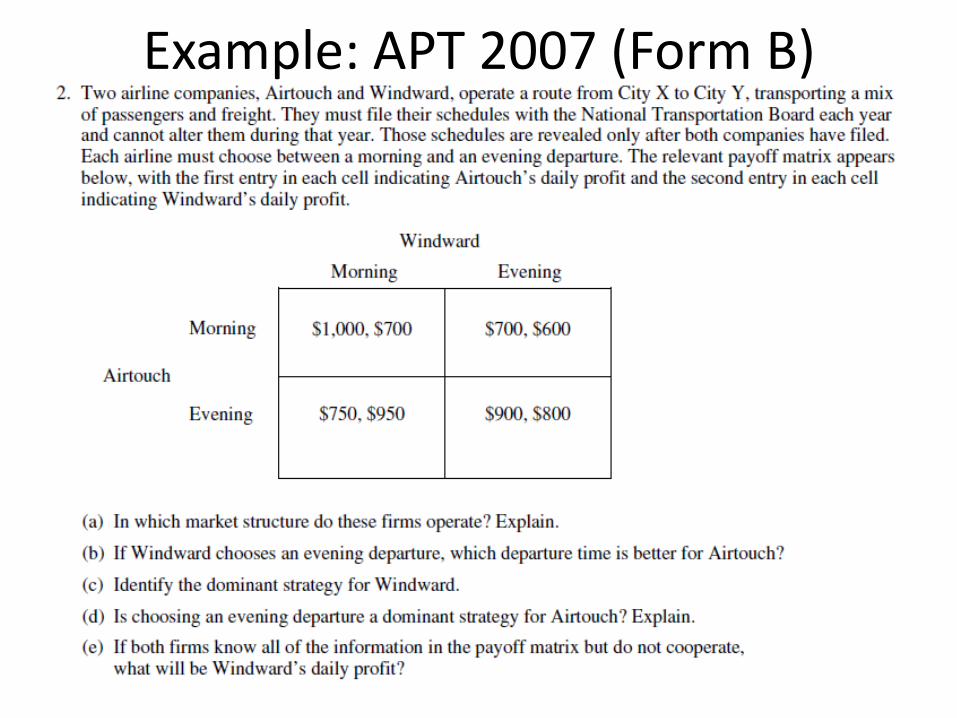
Example: APT 2007 (Form B)

(3,3)
1
2
2
(4,2)
(2,4)
(1,1)
Nash equilibrium (4,2)
(3,3)
2
1
2
1
(2,4)
(4,2)
(1,1)
Nash equilibrium (2,4)
Sequential moves games: example

Strategic Entry Deterrence
Suppose that before the game the incumbent invests in extra capacity, that is not used when he is not challenged, but can be used in case of entry.
Strategic entry deterrence - behavior by incumbent firms to make entry less likely.
Potential entry affects behaviour of incumbent firms: they can erect entry barriers.
Credible threat – a threat to take an action that is in the threatener’s interest to carry out.

Sequential moves game: example

Collusion as a cooperative equilibrium
Q
Р, МR, MC
MC D
c
a
0

Application of prisoners’ dilemma: Oligopoly and collusion
Firm 2
competes
(produces high)
Firm 2 colludes
(produces low)
Firm 1
competes
(produces high)
1 1
3 0
Firm 1 colludes
(produces low)
0 3 2 2

P,MR,MC
Q 0
P*
MR1
MC D1
Q*
D2
MR2
A
B
Kinked demand curve and sticky prices Elastic segment of demand: the firm raises the price
and competitors neglect it. Inelastic segment of demand: the firm reduces the price
and competitors follow.
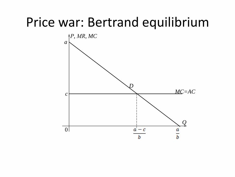
Price war: Bertrand equilibrium
Q
Р, МR, MC
MC=AC
D
c
a
0