monopoly part 2. pricing with market power price discrimination first degree price discrimination...
TRANSCRIPT

Monopoly Part 2Monopoly Part 2

Pricing with Market PowerPricing with Market Power
Price DiscriminationPrice Discrimination
First Degree Price DiscriminationFirst Degree Price Discrimination
Second Degree Price DiscriminationSecond Degree Price Discrimination
Third Degree Price DiscriminationThird Degree Price Discrimination

AR, AC, P
Q
D = AR
MC
MR
Q1
MP1
Q2 Q3
T
N
P3
P2
O
Capturing Consumer SurplusCapturing Consumer Surplus
AR, AC, P
Q
D = AR
MC
MR
Q1
MP1
Q2 Q3
T
N
P3
P2
O
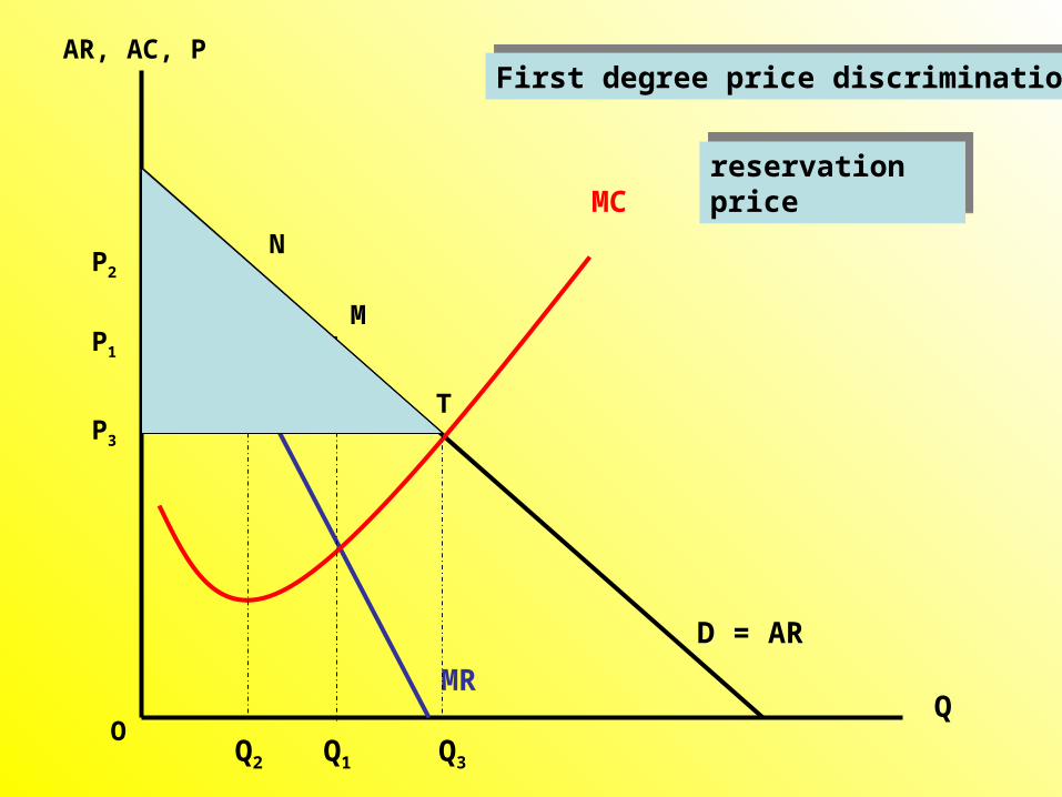
First degree price discriminationFirst degree price discrimination
reservation pricereservation price

AR, AC, P
Q
D = AR
MC
MR
Q1
MP1
Q2
TP2
O
D
E
C
F
BA

ExerciseExercise
Suppose a monopolist has a constant marginal cost MC = 2. The firm faces the demand curve P = 20 – Q. There are no fixed cost.
Suppose a monopolist has a constant marginal cost MC = 2. The firm faces the demand curve P = 20 – Q. There are no fixed cost.
Suppose price discrimination is not allowed. How large will the producer surplus be?
Suppose price discrimination is not allowed. How large will the producer surplus be?
Suppose the firm can engage in perfect first degree price discrimination. How large will be producer surplus be?
Suppose the firm can engage in perfect first degree price discrimination. How large will be producer surplus be?

AR, AC, P
Q
D = AR
Q1
MP2
Q2
TP3
O
N
P1
Q3
Second degree price discriminationSecond degree price discrimination
block pricingblock pricing

AR, AC, P
Q
D = AR
MC
MR
Q0
MP0
Q1 Q3
T
N
P3
P1
O
AC
Q2
P2
R
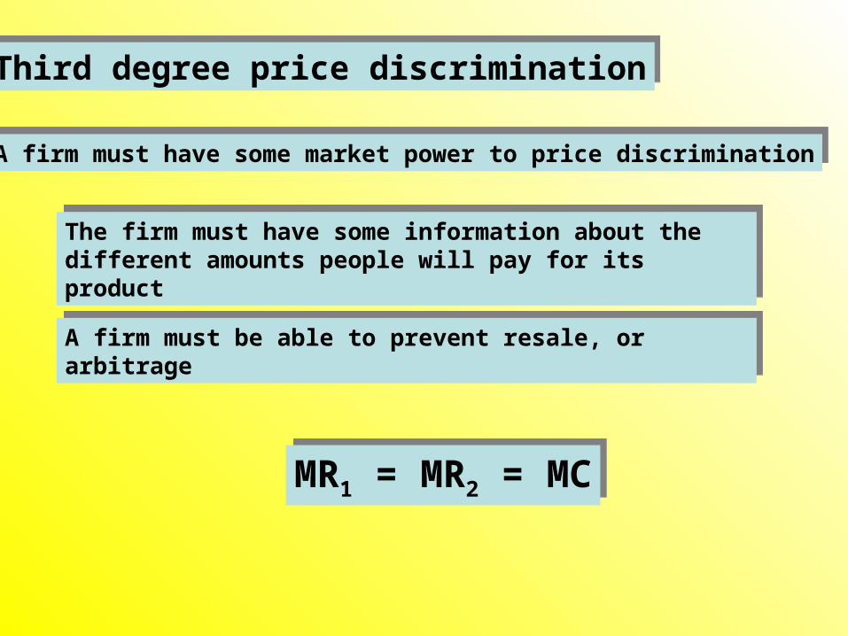
Third degree price discriminationThird degree price discrimination
A firm must have some market power to price discriminationA firm must have some market power to price discrimination
The firm must have some information about the different amounts people will pay for its product
The firm must have some information about the different amounts people will pay for its product
A firm must be able to prevent resale, or arbitrage A firm must be able to prevent resale, or arbitrage
MR1 = MR2 = MCMR1 = MR2 = MC
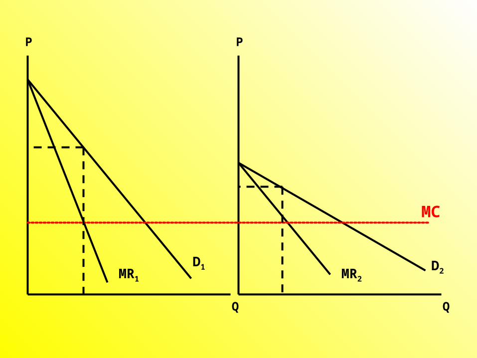
Q
P
Q
P
MC
D1MR1
D2MR2

1 1 2 2 Tπ=PQ +P Q -C(Q )1 1 2 2 Tπ=PQ +P Q -C(Q )
1 1 T
1 1 1
PQ C(Q )π= - 0
Q Q Q
1 1 T
1 1 1
PQ C(Q )π= - 0
Q Q Q
T 1 2Q =Q +QT 1 2Q =Q +Q
2 2 T
2 2 2
P Q C(Q )π= - 0
Q Q Q
2 2 T
2 2 2
P Q C(Q )π= - 0
Q Q Q
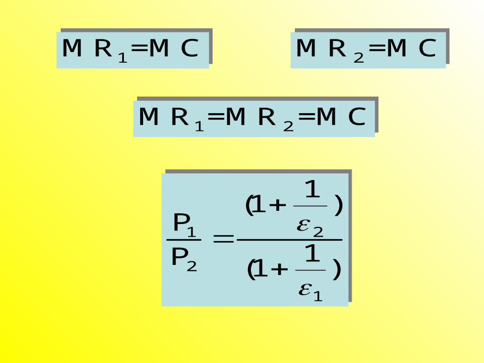
1MR =MC1MR =MC 2MR =MC
2MR =MC
1 2MR =MR =MC1 2MR =MR =MC
1 2
2
1
1(1 )
P1P (1 )
1 2
2
1
1(1 )
P1P (1 )

ExerciseExercise
Suppose a railroad faces the following demand for coal movement
Pc = 38 – Qc Where Qc is the amount of coal moved when the transport price for coal is Pc.
The railroad’s demand for grain movement is PG = 14 – 0.25QG
where QG is the amount of grain shipped when the transport price for grain is PG.
The marginal cost for moving either commodity is 10.
Suppose a railroad faces the following demand for coal movement
Pc = 38 – Qc Where Qc is the amount of coal moved when the transport price for coal is Pc.
The railroad’s demand for grain movement is PG = 14 – 0.25QG
where QG is the amount of grain shipped when the transport price for grain is PG.
The marginal cost for moving either commodity is 10.What are the profit maximizing rates for coal and grain movement?
What are the profit maximizing rates for coal and grain movement?

Intertemporal Price Discrimination Intertemporal Price Discrimination
Q
P
Dt
Dt+1
MRt+1
MRt
Qt
Pt
Qt+1
Pt+1

Peak – Load PricingPeak – Load Pricing
Q
P
D2
D1
MR1
MR2
Q2
P2
Q1
P1
MC

Peak – Load Pricing & WelfarePeak – Load Pricing & Welfare
Q
P
D2
D1
Q2
P2
Q1
P1
MC
P
Q1*Q2
*

Two Part TariffTwo Part Tariff
Q
P
MCP
Usage Fee Entry Fee
Entry Fee

Two Part TariffTwo Part Tariff
Q
P
MCB
D2D1
A
P
T
Q2 Q1
C
Profit = 2T + ( P – MC )(Q1 + Q2 )Profit = 2T + ( P – MC )(Q1 + Q2 )
Two ConsumersTwo Consumers

BundlingBundling
Three VENUS
10,000
A 12,000 3,000
4,000B
Three VENUS
10,000
A 12,000 4,000
3,000B
Negative correlated
Positive correlated

Separated priceSeparated price
Buy BothBuy only good 2
Buy only good 1Buy neither
P2
P1
R1
R2

Bundled priceBundled price
Buy Both
Buy neither
P2
P1
R1
R2
R2= PB – R1

Bundled priceBundled price
Buy Both
Buy neither
P2
P1
R1
R2
R2= PB – R1

Bundled priceBundled price
Buy Both
Buy neither
P2
P1
R1
R2
R2= PB – R1

AdvertisingAdvertising
π=PQ(P,A)-C(Q)-Aπ=PQ(P,A)-C(Q)-A
Adv
Q(P,A) QMR =P =1+MC
A A
Adv
Q(P,A) QMR =P =1+MC
A A
MRAdv = full Marginal cost of Ad.MRAdv = full Marginal cost of Ad.

Q(P,A)(P-MC) =1
A
Q(P,A)
(P-MC) =1A
A Q(P,A) A(P-MC) =
Q A PQ
A Q(P,A) A(P-MC) =
Q A PQ
A
P
εA=-
PQ εA
P
εA=-
PQ ε
Advertising to sale ratio

Transfer PricingTransfer Pricing
No Outside MarketNo Outside Market
Division 1Division 1 Division 2Division 2
Division XDivision X
Q2 , P2Q1 , P1
Q , P
Firm X
Q = f ( K, L, Q1, Q2 )

x 1 1 2(Q)=R(Q)-C (Q)-C (Q )-C (Q)x 1 1 2(Q)=R(Q)-C (Q)-C (Q )-C (Q)
1 x 1 1NMR =(MR-MC )MP =MC1 x 1 1NMR =(MR-MC )MP =MC
2 x 2 2NMR =(MR-MC )MP =MC2 x 2 2NMR =(MR-MC )MP =MC
For FirmFor Firm

1 1 1 1 1=PQ -C (Q )1 1 1 1 1=PQ -C (Q )
2 2 2 2 2=P Q -C (Q )2 2 2 2 2=P Q -C (Q )
x 1 1 2 2π(Q)=R(Q)-C (Q)-PQ -P Qx 1 1 2 2π(Q)=R(Q)-C (Q)-PQ -P Q
x 1 1 1(MR-MC )MP =MC =Px 1 1 1(MR-MC )MP =MC =P
x 2 2 2(MR-MC )MP =MC =Px 2 2 2(MR-MC )MP =MC =P

Race Car Motors has the following demand for automobile
P = 20,000 – Q
MR = 20,000 – 2QDownstream division cost of assembling cars is
CA( Q ) = 8000Q
MCA = 8000The upstream division cost of producing engines is
CE( QE ) = 2QE2
MCE ( QE ) = 4QE
Race Car Motors has the following demand for automobile
P = 20,000 – Q
MR = 20,000 – 2QDownstream division cost of assembling cars is
CA( Q ) = 8000Q
MCA = 8000The upstream division cost of producing engines is
CE( QE ) = 2QE2
MCE ( QE ) = 4QE
ExerciseExercise

MonopsonyMonopsony
Monopsony is a market consisting of single buyer that can purchase from many sellers.Monopsony is a market consisting of single buyer that can purchase from many sellers.
Some buyers may have Monopsony power : a buyer’s ability to affect the price of a good. Monopsony power enables the buyer to purchase the good for less than the price that would prevail in the competitive market
Some buyers may have Monopsony power : a buyer’s ability to affect the price of a good. Monopsony power enables the buyer to purchase the good for less than the price that would prevail in the competitive market

Competitive Buyer & Competitive SellerCompetitive Buyer & Competitive Seller
AR, P
Q
D = MV
MC
AR, P
Q
ME = AEP*
Q*Q*
AR = MR

Monopsonist BuyerMonopsonist BuyerAR, AC, P
MV
ME
QM
PM
QC
S = AE
PC
AR, AC, P
MV
ME
QM
PM
QC
S = AE
PC
AR, AC, P
ARMR
QM
PM
QC
MC
PC
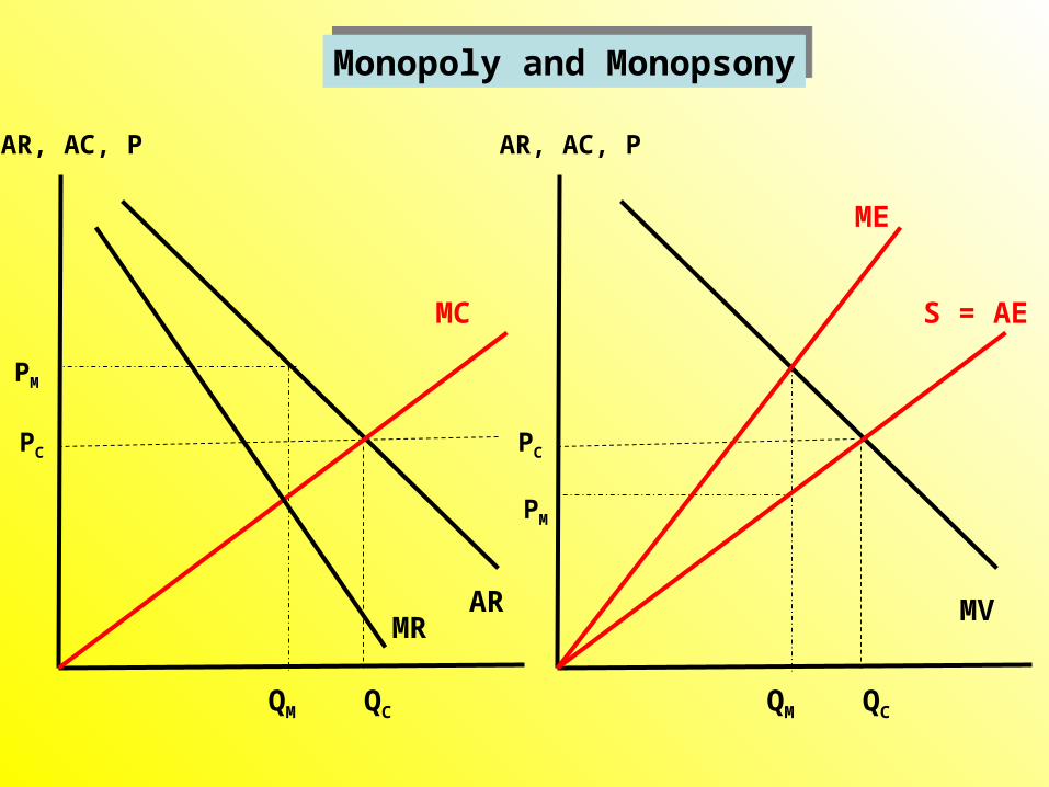
Monopoly and MonopsonyMonopoly and Monopsony

AR, AC, P
AR, AC, P
MV
ME
Q*
P*
S = AE
MV
ME
Q*
MV – P*
S = AE
P*
MV – P*

Source of Monopsony PowerSource of Monopsony Power
The Elasticity of Market SupplyThe Elasticity of Market Supply
The Number of BuyerThe Number of Buyer
The Interaction among BuyersThe Interaction among Buyers

AR, AC, P
MV
ME
QM
PM
QC
S = AE
PCA
B
C
Deadweight LossDeadweight Loss