monte carlo hidden markov models - robotics institute · of baum-welch, and early stopping is...
TRANSCRIPT

Monte Carlo Hidden Markov Models
Sebastian Thrun and John Langford
December 1998CMU-CS-98-179
School of Computer ScienceCarnegie Mellon University
Pittsburgh, PA 15213
Abstract
We present a learning algorithm for hidden Markov models with continuous state and observa-tion spaces. All necessary probability density functions are approximated using samples, alongwith density trees generated from such samples. A Monte Carlo version of Baum-Welch (EM)is employed to learn models from data, just as in regular HMM learning. Regularization duringlearning is obtained using an exponential shrinking technique. The shrinkage factor, which deter-mines the effective capacity of the learning algorithm, is annealed down over multiple iterationsof Baum-Welch, and early stopping is applied to select the right model. We prove that undermild assumptions, Monte Carlo Hidden Markov Models converge to a local maximum in likeli-hood space, just like conventional HMMs. In addition, we provide empirical results obtained in agesture recognition domain, which illustrate the appropriateness of the approach in practice.
This research is sponsored in part by DARPA via AFMSC (contract number F04701-97-C-0022), TACOM (con-tract number DAAE07-98-C-L032), and Rome Labs (contract number F30602-98-2-0137). The views and conclusionscontained in this document are those of the authors and should not be interpreted as necessarily representing officialpolicies or endorsements, either expressed or implied, of DARPA, AFMSC, TACOM, Rome Labs, or the United StatesGovernment.

Keywords: annealing, any-time algorithms, Baum-Welch, density trees, early stopping, EM,hidden Markov models, machine learning, maximum likelihood estimation, Monte Carlo methods,temporal signal processing

Monte Carlo Hidden Markov Models 1
1 Introduction
Over the last decade or so, hidden Markov models have enjoyed an enormous practical success ina large range of temporal signal processing domains. Hidden Markov models are often the methodof choice in areas such as speech recognition [28, 27, 42], natural language processing [5], robotics[34, 23, 48], biological sequence analysis [17, 26, 40], and time series analysis [16, 55]. They arewell-suited for modeling, filtering, classification and prediction of time sequences in a range ofpartially observable, stochastic environments.
With few exceptions, existing HMM algorithms assume that both the state space of the envi-ronment and its observation space are discrete. Some researchers have developed algorithms thatsupport more compact feature-based state representations [15, 46] which are nevertheless discrete;others have successfully proposed HMM models that can cope with real-valued observation spaces[29, 19, 48]. Kalman filters [21, 56] can be thought of as HMMs with continuous state and actionspaces, where both the state transition and the observation densities are linear-Gaussian functions.Kalman filters assume that the uncertainty in the state estimation is alwaysnormally distributed(and hence unimodal), which is too restrictive for many practical application domains (see e.g.,[4, 18]).
In contrast, most “natural” state spaces and observation spaces are continuous. For example,the state space of the vocal tract of human beings, which plays a primary role in the generationof speech, is continuous; yet HMMs trained to model the speech-generating process are typicallydiscrete. Robots, to name a second example, always operate in continuous spaces; hence theirstate spaces are usually best modeled by continuous state spaces. Many popular sensors (cam-eras, microphones, range finders) generate real-valued measurements, which are better modeledusing continuous observation spaces. In practice, however, real-valued observation spaces areusually truncated into discrete ones to accommodate the limitations of conventional HMMs. Apopular approach along these lines is to learn acode-book(vector quantizer), which clusters real-valued observations into finitely many bins, and thus maps real-valued sensor measurements intoa discrete space of manageable size [54]. The discreteness of HMMs is in stark contrast to thecontinuous nature of many state and observation spaces.
Existing HMM algorithms possess a second deficiency, which is frequently addressed in theAI literature, but rarely in the literature on HMMs: they do not provide mechanisms for adaptingtheir computational requirements to the available resources. This is unproblematic in domainswhere computation can be carried out off-line. However, trained HMMs are frequently employedin time-critical domains, where meeting deadlines is essential.Any-timealgorithms [9, 58] addressthis issue. Any-time algorithms can generate an answer at any time; however, the quality of thesolution increases with the time spent computing it. An any-time version of HMMs would enablethem to adapt their computational needs to what is available, thus providing maximum flexibilityand accuracy in time-critical domains. Marrying HMMs with any-time computation is therefore adesirable goal.
This paper presentsMonte Carlo Hidden Markov Models (MCHMMs). MCHMMs employscontinuous state and observation spaces, and once trained, they can be used in an any-time fashion.Our approach employs Monte Carlo methods for approximating a large, non-parametric class ofdensity functions. To combine multiple densities (e.g., with Bayes rule), it transforms sample sets

2 Sebastian Thrun and John Langford
into density trees. Since continuous state spaces are sufficiently rich to overfit any data set, ourapproach uses shrinkage as mechanism for regularization. The shrinkage factor, which determinesthe effective capacity of the HMM, is annealed down over multiple iterations of EM, and earlystopping is applied to choose the right model. We prove the convergence of MCHMMs to a localmaximum in likelihood space. This theoretical results justifies the use of MCHMM in a wide arrayof applications. In addition, empirical results are provided obtained for an artificial domain and agesture recognition domain, which illustrates the robustness of the approach in practice.
The remainder of this paper is organized as follows. Section 2 establishes the basic terminol-ogy for generalizing HMMs to continuous state and observation spaces. We will then, in SectionSection 3, discuss commonly used sampling schemes and provide an algorithm for generatingpiece-wise constant density trees from these samples. A key result in this section is a proof ofasymptotic consistency of both sample-based and tree-based representations. Section 4 describesour approach for complexity control (regularization) using shrinkage, followed by the statement ofthe MCHMM algorithm in Section 5. Section 6 proves the MCHMM convergence theorem, whichstates that under mild assumptions MCHMMs converge with high probability. Empirical resultsare described in Section 7, which specifically investigates MCHMM in the finite sample case. Theempirical results show that MCHMMs work well even in the non-asymptotic case. Section 7 alsoprovides an experiment that characterizes the relation between sample set size (computation) andaccuracy. Finally, related work is discussed in Section 8 and the paper is summarized in Section 9.
2 Generalized Hidden Markov Models
This section introducesgeneralized hidden Markov models(in short: GHMM). GHMMs gener-alize conventional hidden Markov models (HMMs) in that all spaces, state and observation, arecontinuous. Our description closely follows that of Rabiner [43], with densities replacing finiteprobability distributions throughout. Throughout this paper, we assume all event spaces and ran-dom variables (e.g., state, observations) are measurable. We also assume that unless otherwisespecified, all probability distributions are continuous and possess continuous density functions.Further below, when introducing density trees, we will also assume that densities are non-zeroover a compact, bounded region, and that they obey a Lipschitz condition.
A GHMM is a partially observable, time-invariant Markov chain with continuous state and ob-servation spaces and discrete time. Letx denote astate variable(a measurable random variable),defined over some continuous space (e.g.,<k for somek). At each timet � 1, the HMM’s stateis denotedxt. Initially, at timet = 1, the state of the HMM is selected randomly according to thedensity�. State transitions are governed by a conditional probability density, denoted�(x0 j x)and calledstate transition density. Densities are measurable functions over the set of Borel sets,hence the Riemann integralZ x1
x0
�(x0 j x) dx (1)
measures, forx0 < x1, the probabilityPr(x0 � x0 < x1 j x) that the state succeedingx lies in[x0; x1).
In HMMs (and thus in GHMMs), state cannot be observed. Instead, only a probabilistic

Monte Carlo Hidden Markov Models 3
projection of the state is observable. Letbt denote a measurable random variable that models theobservation at timet. Observations are generated according to a probability density conditionedon the state of the HMM (called theobservation density), denoted�(b j x) . If b0 < b1,Z b1
b0
�(b j x) db (2)
measures the probability that the observationb is in [b0; b1), given that the state of the HMM isx.Thus, a generalized HMM is uniquely defined through three densities:
� = f�; �; �g: (3)
Putting computational limitations aside for the moment, knowledge of� is sufficient to tackle avariety of interesting practical problems:
� Computing distributions over states and observations at arbitrary points in time,
� Generating representative example trajectories in state and observation space,
� Determining the likelihood of example trajectories under an HMM, and
� Classifying data sequences generated by mixtures of labeled HMMs.
Algorithms for these problems are described in detail in [43]; they are easily transferred from thefinite to the continuous case.
In practice, the densities� are often unknown and have to be estimated from data. The data,denotedd, is a sequence of observations1 , denoted
d = fO1; O2; : : : ; OT g: (4)
HereOt denotes the observation at timet. The total number of observations ind is T .The well-known Baum-Welch algorithm [2, 33, 43] provides a computationally efficient and
elegant approach for learning�, �, and�. Baum-Welch begins with an initial model, denoted�(0). It iterates two steps, an E-step and an M-step (see also [12]). In then-th E-step, distributionsfor the various state variablesxt are computed under a fixed model�(n) (with n � 0). Then-thM-step uses these distributions to derive a new, improved model�(n+1). As shown for example in[33, 37], both steps increase the data likelihoodPr(d j �), or leave it unchanged if, and only if, alocal maximum in the likelihood function has been reached.
In the E-step, distributions are computed for the state variablesxt conditioned on a fixed model� and the datad. Recall that in the discrete case,
�(n)t (x) = Pr(xt = x j O1; : : : ; Ot; �
(n)) (5)
�(n)t (x) = Pr(Ot+1; : : : ; OT j xt = x; �(n)) (6)
(n)t (x) = Pr(xt = x j d; �(n)) (7)
�(n)t (x; x0) = Pr(xt = x; xt+1 = x0 j d; �(n)) (8)
1For simplicity of the presentation, we only present the case in which the data consist of a single sequence. Theextension to multiple sequences is straightforward but requires additional notation.

4 Sebastian Thrun and John Langford
The continuous case is analogous; however, here� and� are densities, and thus may be larger than1. Following [43], these densities are computed incrementally;� is computed forward in time, and� backwards in time (for which reason this algorithm is often referred to as theforward-backwardalgorithm. Initially,
�(n)0 (x) = �(n)(x) (9)
�(n)T (x) = 1 (10)
and for all other�t and�t:
�(n)t (x) =
Z�(n)t�1(x
0) �(n)(x j x0) �(n)(Ot j x) dx0 (11)
�(n)t (x) =
Z�(n)t+1(x
0) �(n)(x0 j x) �(n)(Ot+1 j x0) dx0 (12)
Bayes rule governs the conditional density over the state space at timet:
(n)t (x) =
�(n)t (x) �
(n)t (x)Z
�(n)t (x0) �(n)t (x0) dx0
(13)
Similarly, the state transition densities�(n) are computed as
�(n)t (x; x0) =
�(n)t (x) �(n)(x0 j x) �(n)(Ot+1 j x0) �(n)t+1(x)Z Z
�(n)t (�x) �(n)(�x0 j �x) �(n)(Ot+1 j �x0) �(n)t+1(�x) d�x d�x0
(14)
This computation is completely analogous to the finite case, replacing conditional probabilities byconditional densities.
The M-step uses (n)t (x) and�(n)t (x; x0) to compute a new model�(n+1), using the maximumlikelihood estimator:
�(n+1)(x) = (n)0 (x) (15)
�(n+1)(x0 j x) =
PT�1t=1 �
(n)t (x; x0)PT�1
t=1 (n)t (x)
(16)
�(n+1)(b j x) =
PTt=1 IOt=b
(n)t (x)PT
t=1 (n)t (x)
(17)
HereIcond denotes an indicator variable that is 1 if the conditioncondis true, and 0 otherwise. Astraightforward result is the convergence of GHMMs under approprate conditions.
Theorem 1. (GHMM Convergence Theorem)If all distributions of a GHMM� possessdensity functions that are Lipschitz (and differentiable) in all variables, then for almost all (mea-sure 1) points the steps outlined above do not decrease the probability density of the observationsequence. They do not improve the probability density of the observation sequence at each iter-ation if, and only if, the distributions at the beginning of an EM step are at a critical point (localmaximum, minimum, or saddle point).

Monte Carlo Hidden Markov Models 5
Proof.Only sketched here (see also [2, 20, 33], and see [47] for an extension to certain real-valued spaces). For finite-state finite-observation HMMs, all densities and variables (�, �, �, �,�, , and�) can be implemented by vectors, and the Baum-Welch algorithm has been proven toconverge [2]. Juang [19] has shown convergence to local maxima for HMMs with a finite numberof states and continuous observations where the observation densities are a mixture of log concaveor ellipsoidal symmetrical densities. In particular, the class of ellipsoidal symmetrical densitiesincludes Gaussians. A GHMM can be viewed as the limit as the number of Gaussians is allowedto increase to infinity, and then the number of states is allowed to increase to infinity in Juang’sanalysis. Since Gaussians meet the assumptions of Juang’s analysis, any continuous�(Ojx) canbe the limit.
limK!1
KXk=1
ckx bkx(O) (18)
whereP
k ckx = 1 andbkx(O) is a Gaussian.Juang’s analysis contains the following forms of manipulation:Z
Y
ZXf(x; y) dx dy =
ZX
ZYf(x; y) dy dx (19)
rY
ZXf(x; y) dx =
ZXrY f(x; y) dx (20)
wheref(x; y) is some function proportional to a density. Differentiability of all densities is asufficient assumption for these statements to hold true. 2
3 Density Approximation
This section describes sample-based and tree-based methods for density approximation. The no-tion of asymptotic consistencyis introduced and results, along with error bounds, are given for apopular sampling algorithm and a tree method. Throughout this section, we assume that all densityfunctions are centered on a compact and bounded region in<k (for an arbitraryk) and that theyare Lipschitz.
3.1 Sampling
Samplesare values drawn from the domain of a density function, where each sample is annotatedby a non-negative real value [30, 36, 57]. Sample sets are (finite) sets of samples, annotated bynumerical probability values. More specifically, letf be a probability density function, and letNdenote a positive number (the cardinality of a sample set). Then asample setis a set
X = fhx1; px1i : : : ; hxN ; pxN ig withNXn=1
pxn = 1 (21)
6 Sebastian Thrun and John Langford
wherexn 2 dom(f) andpxn 2 [0; 1] for all n with 1 � n � N . Sample sets can be thought ofas discrete distributions over the event spacefx1; : : : ; xNg and probability distribution defined byfpx1 ; : : : ; pxN g [36, 41].
One popular sampling method is calledimportance sampling, which was originally introducedby Rubin [44]. Importance sampling approximates a densityf by drawing samplesx from adistribution with densityg, and assigning a weightpx proportional tof(x)
g(x) . Obviously, the densityg must be non-zero over the support off , i.e.,
f(x) > 0 =) g(x) > 0 (22)
We will distinguish two special cases:
1. Likelihood-weighted sampling. If g�f , we will refer to the sampling algorithm aslikelihood-weighted sampling. Here we draw samples according tof and assigns equal probability toeach sample in the sample set [22]:
xn is drawn according tof
pxn = N�1 (23)
In many cases, likelihood-weighted sampling can easily be implemented usingrejection sam-pling [36].
2. Uniform sampling. If g is uniform over (a superset of) the support off , we will call thesampling algorithmuniform sampling. This sampling algorithm draws values randomly (uni-formly) from the support off (which is assumed to be bounded), and assigns to each valuexa probability proportional to its densityf(x):
xn is drawn uniformly fromdom(f)
pxn = f(xn)
"NXi=1
f(xi)
#�1(24)
Uniform sampling covers the domain of a density uniformly regardless of the nature of the densityfunction. Likelihood-weighted sampling populates the space according tof , so that the densityof sample is proportional to the densityf . Likelihood-weighted sampling can be said to “waste”fewer samples in low-likelihood regions off [41]. In other words, ifXu andXlw are sample setsgenerated from the same distribution using uniform sampling, and likelihood-weighted sampling,respectively, the following holds true in expectation:X
hx;pxi2Xu
f(x) �X
hx;pxi2Xlw
f(x) (25)
were the equality holds in expectation if and only iff is uniform [51]. Henceforth, we will focusour attention on likelihood-weighted sampling whenever we have an explicit representation of aprobability distribution (and importance sampling otherwise).

Monte Carlo Hidden Markov Models 7
(a) (b)
Figure 1: (a) Data set (b) partitioned by a density tree.
Figure 1a shows a sample set drawn by likelihood-weighted sampling from a distribution thatresembles the shape of a sine wave in 2D. All probabilitiespx of the sample set shown there arethe same, and the samples are concentrated in a small region of the<2. In practice, likelihood-weighted sampling is often given preference over uniform sampling—specifically if the targetdensity is known to only populate (with non-zero measure) a small subspace of its domain.
Both sampling methods can equally be applied tosample from a sample set(resampling). LetX be a sample set. Under uniform sampling, a new sample set is generated by randomly drawingsampleshx; pxi from X with a uniform distribution (regardless of thepx values). Thepx-valuesin the new sample set are then re-normalized so that they add up to 1. Under likelihood-weightedsampling, samples are drawn fromX according to the (discrete) probability distribution inducedby theirpx-values. Each sample is then assigned the same probability. Sampling from sample setsplays an important role in the Monte Carlo HMM algorithm described below.
3.2 Asymptotic Consistency
The central idea of sampling is torepresentdensity functions by finite sample sets, which are com-putationally advantageous. So what does it mean for a sample setX to “represent” a densityf?Obviously, sample sets represent discrete distributions and thus cannot represent distributions thatpossess densities (hence are continuous). However, we will call a sampling methodasymptoticallyconsistentif for N !1, X converges tof with probability 1 when integrated over the system ofhalf-open Borel sets:
limN!1
Xhx;pxi2X
Ix0�x<x1 px =
Z x1
x0
f(x) dx w.p. 1 (26)
Recall the system of half-open intervals is an inducing system for the sigma algebra over the<k;hence, it suffices to show convergence for those sets.
A key observation is that both sampling algorithms are asymptotically consistent—as are allimportance sampler withf(x) > 0 =) g(x) > 0 [51]. This is formalized for the more im-

8 Sebastian Thrun and John Langford
portant likelihood-weighted sampling technique in the following theorem, which also provides aprobabilistic error bound for the finite case.
Theorem 2.The likelihood-weighted sampling method is asymptotic consistent. For finiteN ," > 0 andx0 < x1, the likelihood that the error between a densityf and a sampleX is larger than" can be bounded as follows:
Pr
0@������X
hx;pxi2XIx0�x<x1 px �
Z x1
x0
f(x) dx
������ > "
1A � 2 e�2"
2N (27)
Thus, according to the theorem the error betweenf and its sample decreases at the familiar rate1pN
.
Proof. The convergence follows directly from the Central Limit Theorem (see also [13, 41,51]). The bound follows from the Hoeffding bound, under the observation that for any half-open interval[x0; x1) each sample can be viewed as a zero-one “guess” of the size of the areaR x1x0
f(x) dx. 2
More generally, the convergence rate of importance sampling is inO( 1pN) if f(x)
g(x) <1. Thevariance of the error depends on the “mismatch” betweenf andg (see e.g., [51], pg. 33). TheNwill be reduced by a constant factor ofmaxx
f(x)g(x) <1 for appropriateg(x).
3.3 Density Trees
While sample sets are sufficient to approximate continuous-valued distributions, they differ fromthose in that they arediscrete, that is, even in the limit they assign non-zero likelihood to onlya countable number of points. This is problematic if one wants tocombinedensities representedthrough different sample sets: For example, letf and g be two density functions defined overthe same domain, and letX be a sample off andY a sample ofg. Then with probability 1,none of the samples inX andY are identical, and thus it isnot straightforward how to obtain anapproximation of their productf � g from X andY . Notice that multiplications of densities arerequired by the Baum-Welch algorithm (see e.g., Equation (13)).
Density trees, which are quite common in the statistical literature [24, 35, 38, 39], transformsample sets into density functions. Unfortunately, not all tree growing methods are asymptoti-cally consistent when applied to samples generated from a densityf . We will describe a simplealgorithm which we will prove to be asymptotically consistent.
Our algorithm annotates each node in the tree with a hyper-rectangular subspace ofdom(f),denoted byV (or Vi for the i-th node). Initially, all samples are assigned to the root node, whichcovers the entire domain off . A nodei is split whenever the following two conditions are fulfilled:
1. At leastpN sampleshx; pxi 2 X fall into in Vi.
2. Its depth, i.e., its distance from the root node, does not exceedb14 log2Nc.
If a node is split, its intervalv is divided into two equally sized intervals along its longest dimen-sion. These intervals are assigned to the two children of the node. Otherwise, a node becomes aleaf node of the density tree.
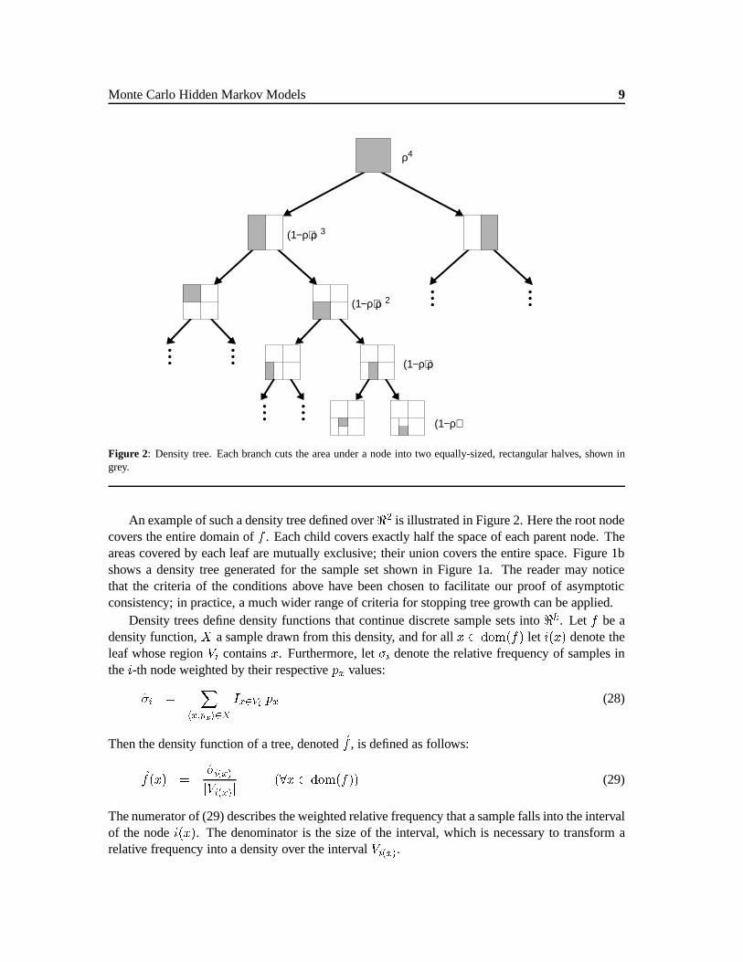
Monte Carlo Hidden Markov Models 9
... ...
... ...... ... (1−ρ)
(1−ρ) ρ
(1−ρ) ρ2
(1−ρ) ρ3
ρ4
Figure 2: Density tree. Each branch cuts the area under a node into two equally-sized, rectangular halves, shown ingrey.
An example of such a density tree defined over<2 is illustrated in Figure 2. Here the root nodecovers the entire domain off . Each child covers exactly half the space of each parent node. Theareas covered by each leaf are mutually exclusive; their union covers the entire space. Figure 1bshows a density tree generated for the sample set shown in Figure 1a. The reader may noticethat the criteria of the conditions above have been chosen to facilitate our proof of asymptoticconsistency; in practice, a much wider range of criteria for stopping tree growth can be applied.
Density trees define density functions that continue discrete sample sets into<k. Let f be adensity function,X a sample drawn from this density, and for allx 2 dom(f) let i(x) denote theleaf whose regionVi containsx. Furthermore, let�i denote the relative frequency of samples inthei-th node weighted by their respectivepx values:
�i =X
hx;pxi2XIx2Vi px (28)
Then the density function of a tree, denotedf , is defined as follows:
f(x) =�i(x)jVi(x)j
(8x 2 dom(f)) (29)
The numerator of (29) describes the weighted relative frequency that a sample falls into the intervalof the nodei(x). The denominator is the size of the interval, which is necessary to transform arelative frequency into a density over the intervalVi(x).
10 Sebastian Thrun and John Langford
The density functionf(x) can be equally defined forinternal nodes(non-leaf nodes). This willbe important below, where estimates at different levels of the tree are mixed for regularization.
3.4 Asymptotic Consistency of Density Trees
An important result is the asymptotic consistency of density trees. This result, which justifiesthe use of density trees are non-parametric approximation, will be formalized in the followingtheorem:
Theorem 3. Density trees are asymptotically consistent, that is, for allx0; x1 2 dom(f) withx0 < x1 and for any density treef(x) generated from a sample setX generated from a densityf ,the following holds true:
limN!1
Z x1
x0
f(x) dx =
Z x1
x0
f(x) dx w.p. 1: (30)
We will first prove a related result, namely that of pointwise stochastic convergence
limN!1
f(x) = f(x) (8x 2 dom(f)) w.p. 1 (31)
which under the assumptions made in this paper implies the theorem. The proof is carried out intwo stages, each of which is described by its own lemma.
Lemma 1. The densityf converges to a function�f which is defined through the same tree asf , but with the weighted relative frequencies�i replaced by their true frequencies, denoted��i:
��i =
ZVi
f(x) dx: (32)
Lemma 2. The densityf converges tof .Proof of Lemma 1.For each leafi, the Hoeffding bound states that
Pr(j ��i � �ij > ") < 2 e�2"2N : (33)
Our tree growing rule limits the depth of the tree tob14 log2Nc. Hence, there are at most
21
4log2N = N
1
4 (34)
nodes in the tree. Thus, the probability that there exists a leaf whose empirical frequency�ideviates from the true probability��i is bounded by
Pr(9 leaf i : j ��i � �ij > ") < 2 N1
4 e�2"2N : (35)
The error of the empirical frequency estimates is now translated into density errors. Recall thataccording to (29), the relative frequency is related to the density of a tree by the volumeVi of eachleaf. Consequently,
j �f(x)� f(x)j = jVij�1 j ��i � �ij (36)

Monte Carlo Hidden Markov Models 11
Observing that the volume of the interval covered by a leafjVij is at leastN� 1
4 —which directlyfollows from the depth limit imposed when growing density trees—we obtain
j �f(x)� f(x)j � N� 1
4 j ��i � �ij (37)
() N1
4 j �f(x)� f(x)j � j ��i � �ij (38)
Substituting this into (35) yields:
Pr(j �f(x)� f(x)j > N1
4 ") < 2 N1
4 e�2"2N ; (39)
which with the substitution"0 = N1
4 " leads to the following error bound betweenf and �f :
Pr(j �f(x)� f(x)j > "0) < 2 N1
4 e�2"02pN : (40)
Obviously, the right hand-size of (40) converges to 0 asN !1, which proves pointwise conver-gence off to �f . 2
It remains to be shown that�f converges off .Proof of Lemma 2.It suffices to show that with high likelihood, any leafi that covers an inter-
val with non-zero measure, i.e.,
��i > 0 (41)
will be split infinitely often asN is increased. The desired convergence then follows directly fromthe fact thatf obeys a Lipschitz condition. The proof is given for likelihood-weighted sampling.
Let i be a leaf node, and letdepth(i) denote its depth. Furthermore, letni be the number ofsamples in nodei:
ni =X
hx;pxi2XIx2Vi = N �i (42)
The second equality exploits the assumption that samples are generated by likelihood-weightedsampling. Recall that the nodei is split if ni �
pN , for sufficiently largeN . Without loss of
generality, let us assume that
N > max
�1
(��i � ")2; 4depth(i)
�and " < ��i (43)
The second term in the max ensures that the depth limitb14 log2Nc in the tree growing rule doesnot restrict splitting nodei. The other assumptions (43) imply that
��i >1pN
+ " (44)
The Hoeffding bound now yields the desired result:
Pr(��i � �i > ") � e�2"2N (45)
=) Pr
�1pN
+ "� �i > "
�� e�2"
2N (46)

12 Sebastian Thrun and John Langford
() Pr
�1pN
> �i
�� e�2"
2N (47)
() Pr
�1pN
>niN
�� e�2"
2N (48)
() Pr�p
N > ni�
� e�2"2N (49)
Thus, with high probabilityni �pN and nodei is split. The pointwise convergence of�f to f
now follows from our assumption thatf is Lipschitz. 2
Proof of the Theorem 3.We have already shown that
limN!1
f(x) = f(x) w.p. 1 and8x 2 dom(f): (50)
Theorem 3 follows trivially from the triangle inequality, sincedom(f) is bounded and Lipschitz(which implies thatf is bounded). 2
The termination conditions for growing trees (see itemized list in Section 3.3) where chosento facilitate the derivation of Theorem 3. In practice, these conditions can be overly restrictive,as they often require large sample sets to grow reasonable-sized trees. Our actual implementationsidesteps these conditions, and trees are grown all the way to the end. While the convergenceresults reported here are not applicable any longer, our implementation yielded much better per-formance specifically when small sample sets were used (e.g., 100 samples).
4 Regularization Through Shrinkage and Annealing
We will now resume our consideration of GHMMs. The continuous nature of the state space inGHMMs, if represented by arbitrary sample sets and/or trees, can easily overfitany data set, nomatter how large. This is because GHMMs are rich enough to assign a different state to eachobservation in the training data (of which there are only finitely many), making it essentiallyimpossible to generalize beyond sequences other than the ones presented during training. A similarproblem arises in conventional HMMs, if they are given more states than samples in the data set.In GHMMs the problem is inherent, due to the topology of continuous spaces. Thus, some kindof regularization is needed to prevent overfitting from happening.
Our approach to regularization is based onshrinkage[50]. Shrinkage is a well-known statisti-cal technique for “lumping together” different estimates from different data sources. In a remark-able result by Stein [50], shrinking estimators were proven to yield uniformly better solutions overunbiased maximum-likelihood estimators in multivariate Gaussian estimations problems (see also[53]). Shrinkage trees were introduced in [32]. Instead of using the density estimates at the leafsof a tree, shrinkage trees mix those densities with densities obtained further up in the tree. Theseinternal densities are less specific to the region covered by a leaf node; however, their estimatesare usually obtained from more data, making them less susceptible to variance in the data.
Figure 3 shows an example using shrinkage with an exponential factor, parameterized by�(with 0 � � � 1). Here each node in the tree, with the exception of the root node, weighs itsown density estimate by(1 � �), and mixes it with the density estimate from its parent using theweighting factor�. As a result, every node along the path contributes to the density estimate at the

Monte Carlo Hidden Markov Models 13
... ...
... ...... ... (1−ρ) σm
(1−ρ) ρ σl
(1−ρ) ρ2 σk
(1−ρ) ρ3 σj
ρ4 σi
node i
node j
node k
node l
node m
Figure 3: Shrinkage for complexity control. The density of each node is an exponentially weighted mixture of densitiesof the nodes along the path to the leaf. Shown here is an example for nodem, whose path leads through nodesi, j, k,andl. The�-terms describe the mixture coefficients for this example. If� is 0, only the leaf estimate is used. For largervalues of�, estimates from data beyond the leaf data are used to estimate the target density.
leaf; however, its influence decays exponentially with the distance from the leaf node. Obviously,the value of� determines the amount of shrinkage. If� = 1, only the root node is consulted,hence, the probability density induced by the tree is uniform. If� = 0, on the other hand, there isno shrinking and only the estimates in the leaf nodes determine the shape of the density function.For intermediate values of�, estimates along the entire path are combined.
Since the optimal value of� is problem-specific—de facto it depends on the nature of the(unobservable) state space—our approach uses annealing and cross validation to determine thebest value for�. More specifically,
�(n) = ��n�1 (51)
where �� < 1 is a constant (e.g., 0.9) andn denotes the iteration counter of the Baum-Welchalgorithm (starting at 1). Thus,� starts with�(0) = 1, for which nothing can be learned, sinceevery density is uniform. The parameter� is then annealed towards zero in an exponential fashion.Cross validation (early stopping) is applied to determine when to stop training.

14 Sebastian Thrun and John Langford
Table 1: The MCHMM algorithm at-a-glance.
Model Initialization: Initialize � = f�; �; �g by three randomly drawn sets of samples of the appropriatedimension. Generate density trees from these samples. Set� = 1, and chose an initial sample set sizeN > 0.
E-step:
1. Copy the sample set representing� into�0 (c.f., (9)).
2. Set�T = 1.
3. Computation of�t (c.f., (11)). For eacht with 1 < t � T do:
(a) GenerateN sampleshx0; px0i from the sample set representing�t�1 using likelihood-weighted sampling.
(b) For each samplehx0; px0i, generate the conditional density�(x j x0) using the tree-version of�. Sample a singlex from this tree, using likelihood-weighted sampling.
(c) Setpx to a value proportional to�(Ot j x), whereOt is thet-th observation in the data set.This density value is obtained using the tree representing�.
(d) Generate a tree from the new sample set.
4. Computation of�t (c.f., (12)). For eacht with 1 � t < T do:
(a) GenerateN sampleshx0; px0i from the sample set representing�t+1 using likelihood-weighted sampling.
(b) For each samplehx0; px0i, generate the conditional density�(x0 j x) using the tree-version of�. Sample a singlex from this tree, using likelihood-weighted sampling.
(c) Setpx to a value proportional�(Ot+1 j x0), whereOt+1 is thet+1-th observation in the data
set. This density value is obtained using the tree representing�.(d) Generate a tree from the new sample set.
5. Computation of t (c.f., (13)). For eacht with 1 � t � T do:
(a) GenerateN=2 sample from�t by likelihood weighted sampling and assign to each samplehx; pxi a probability proportional to�t(x), using the tree approximation of�t.
(b) GenerateN=2 sample from�t by likelihood weighted sampling and assign to each sampledhx a probabilitypx proportional to�t(x), using the tree approximation of�t.
M-step:
1. Estimation of the new state transition density� (c.f., (16)): PickN random timest 2 f1; : : : ; T�1gand generate sampleshx; pxi andhx0; px0i from t, and t+1, respectively, by likelihood-weightedsampling. Addh(x; x0); N�1i into the sample set representing�. Generate a tree from the sampleset.
2. Estimation of the new observation density� (c.f., (17)): PickN randomt 2 f1; : : : ; Tg andgenerate a samplehx; pxi from t by likelihood-weighted sampling. Addh(x;Ot); N
�1i into thesample set representing�. Generate a tree from the sample set.
3. Estimation of the new initial state distribution� (c.f., (15)): Copy the sample set 0 into�. Generatea tree from the sample set.
Annealing: Set� ���. Stop when the likelihood of an independent cross-validation set is at its maxi-mum.
Sample set size:IncreaseN .

Monte Carlo Hidden Markov Models 15
5 Monte Carlo HMMs
We are now ready to present the main algorithm of this paper, along with the main theoreticalresult: The Monte Carlo algorithm for GHMMs, calledMonte Carlo hidden Markov models(inshort MCHMM). A MCHMM is a computational instantiation of a GHMM that represents alldensities through samples and trees. It applies likelihood-weighted sampling for forward andbackward projection (c.f., Equations (11) and (12)), and it uses annealing and cross-validation todetermine the best shrinkage factor. To ensure convergence, the number of samplesN is increasedover time.
The learning algorithm for MCHMM is depicted in Table 1. MCHMMs use both sample-based and tree representations during learning. After learning, it suffices to store only the tree-based version of the model� = f�; �; �g; all sample sets can be discarded. When applyinga trained MCHMM to a new data set (e.g., for analysis, prediction, or classification), only the“forward” densities�t(x) have to be estimated (just like in conventional HMMs, Kalman filters[21, 31], or dynamic belief networks [8, 45]). For that, no trees have to be grown. Instead,samples for�t+1(x) are obtained by sampling from the sample set representing�t(x) (see alsoSection 3.1) and the tree representing�. Thepx-values of�t+1(x) are determined using the treerepresenting�. This recursive resampling technique, known as sampling/importance resampling[44, 49] applied to time-invariant Markov chains, converges at the rate1=
pN (if T is finite, c.f.,
Section 3.2). Sampling/importance resampling, which will further be discussed in Section 8, hasbeen successfully applied in domains such as computer vision and robotics [11, 18].
6 Error Analysis and Convergence Results
This section presents the major convergence result for MCHMM. Under mild assumptions, MCH-MMs can be shown to converge with probability 1 to models� that locally maximize likelihood;just like conventional HMMs. The proof builds on the well-known results for discrete HMMs (seeg.e., [2, 19, 20, 33, 47]), and shows that if the sample sizeN is sufficiently large, the deviationbetween the MCHMMM and the corresponding GHMM can be bounded arbitrarily tightly withhigh probability, exploiting the asymptotic consistency of the two major approximations: samplesand density trees.
6.1 Relative Error
The process of Monte Carlo simulation introduces error into the Baum-Welch algorithm. In orderto understand how this affects convergence, we need to understand how an initial error will prop-agate through an EM step. This analysis will also cover errors introduced in the middle of an EMstep as long as such errors converge to 0 with large samples, because errors introduced in mid-stepwill be indistinguishable from an error introduced at the beginning of the calculation.
What we would like to prove is that a small absolute initial error will imply a small absolutefinal error. Unfortunately, this is not possible because several calculations are normalized integralsof products. Consider the integral
Rx f(x)g(x)dx. If f(x) = step(x� 1=2) andg(x) = 1� f(x)
thenRx f(x)g(x) dx = 0. However, if �f(x) = f(x) + " and�g(x) = g(x) + " are integrated, we

16 Sebastian Thrun and John Langford
get a non-zero integral:R 1x=0
�f(x)�g(x)dx = ". First, notice that the calculation of�t(x) is of thisform. Assume, for the moment, that�t(x) = 1. Then t(x) = �t(x)=
R�t(x
0)dx0. Consequently,if �t(x) was small (< ") everywhere,� t(x) can potentially be very far from t(x). Furthermore,any allowable error can produce an arbitrarily large error in the output.
However, if we have a smallrelativeerror,
�f(x)� f(x)
f(x)< " (52)
we will be able to prove that a small initial error implies a small final error. The restriction tosmall relative error is significant because density trees only guarantee a small absolute error. Anextra assumption must be placed on the initial distribution in order to guarantee that the densitytree produced by sampling from the distribution will have small relative error.
To simplify the proof that a small initial error produces a small final error, we only considertransforming functions to first order,f(�x) � f 0(x)(�x� x). There is no zeroth order error becausethe limit as the relative error approaches0 is f(x), lim�x!x f(�x) = f(x). Higher order errorbecomes small quickly for all transforming functions which we consider. Consequently, we willbe able to state that for all"; �, there exists some number of samples,N , s.t. f(�x) � f(x) �f 0(x)(�x� x) + " with probability1� �.
Our analysis does not consider the shrinkage factor�, which, sincelimn!1 �(n) = 0, hasasymptotically no effect.
6.2 Convergence of MCHMMs
We will now state the central result of this section: the MCHMM convergence theorem and animportant corollary. The proof of the theorem will be developed throughout the remainder of thissection.
Theorem 4 (MCHMM Convergence Theorem).If approximation of the underlying distribu-tions by density trees causes only a finite relative error which decreases to0 asN !1 and an EMstep in a GHMM starting with�(n); �(n); �(n) produces output distributions�(n+1); �(n+1); �(n+1)
then for all"; � there exists anN s.t. the output of an MCHMM iteration taking�(n); �(n); �(n) asinputs with probability1�� satisfiesj�(n+1)(x)��0(n+1)(x)j < ", j�(n+1)(x0jx)��0(n+1)(x0jx)j <", andj�(n+1)(Otjx)� �
0(n+1)(Otjx)j < " where�0(n+1), �
0(n+1), and�0(n+1) are the output dis-
tributions of the MCHMM iteration.The proof of Theorem 4 will be presented below, after introducing a collection of useful lem-
mas. However, Theorem 4 implies the following important corollary:Corollary. Under the same assumptions as in Theorem 4, any strictly monotonically increas-
ing schedule ofN ’s will cause a MCHMM to converge to a local maximum in with probability1.
Proof of the corollary.The convergence of GHMMs is a straightforward extension of the well-known convergence proof for HMMs as outlined in the proof of Theorem 1. The action of aGHMM iteration causes movement through the space of distributions. We can view this action ofa GHMM iteration as inducing a vector field in the (infinite dimensional) space of distributionswith a magnitude proportional to the change in likelihood and a direction given by�(n)(x; x0) �

Monte Carlo Hidden Markov Models 17
�(n+1)(x; x0). The action of an MCHMM with probability1� � will have a result in a perturbedvector with the error bounded by". The repeated action of a MCHMM with N increasing willcreate a Cauchy sequence where the" decreases to0 and� decreases to0. This Cauchy sequencewill limit to local maxima with probability 1. 2
It is important to notice that this corollary doesnotstate that an MCHMM and GHMM startingwith the same distribution will converge to thesamelocal maximum. Such a result will gener-ally not hold true, as the finiteness ofN might influence the specific local maximum to which aMCHMM converges.
It is also interesting to note that the noise introduced by MCHMMs in the convergence stepmay be beneficial. The argument is informal because the noise of an MCHMM has both systematic(due to representation) and random (due to sampling) effects. First, consider a GHMM whichaccidentally starts out at a local minimum (or a saddle point). The GHMM might be stuck here,but a MCHMM will, with probability 1, step off of the local minima and move towards a localmaxima. In addition, consider a landscape containing many local maxima on it’s flanks. A GHMMcould easily become trapped in a local maxima while an MCHMM with a lowN will be kickedout of the local maxima with high probability. In this way, an MCHMM could gain some of thebenefits of simulated annealing.
6.3 Propagation of Error
Before we can prove the MCHMM convergence theorem, we will need to develop an analysis ofthe propagation of errors through transforming functions.
Let us start by assuming that we have some initial error�(x) = �(x) + ��(x), �(xjx0) =�(xjx0) + ��(x; x
0) and�(Otjx) = �(Otjx) + ��(Ot; x). These errors can, for example, be theerrors introduced by approximating a distribution with density trees. It will also be convenient totalk about the relative error
�r�(x) =
������(x)
�(x)
���� (53)
�r�(xjx0) =
������(xjx0)�(xjx0)
���� (54)
�r�(Otjx) =
������(Otjx)�(Otjx)
���� (55)
�rf (y) =
�����f (y)
f(y)
���� (56)
and the largest relative error over the input range
�r� = max
x�r�(x) (57)
�r� = max
x;x0�r�(xjx0) (58)
�r� = max
x;Ot
�r�(Otjx) (59)
�rf = max
y�rf (y) (60)
18 Sebastian Thrun and John Langford
The propagation of errors through individual calculations of Baum-Welch will be characterized bytaking a derivative. Let�x = x+�(x). The definition of a derivative isd
dxf(x) = lim�x!x
f(�x)�f(x)�x�x .
As the difference between 2 distributions,�x andx approaches0, the difference between the re-sulting calculations,f(�x) andf(x), will approachf 0(x)�(x) implying �f (x) = f(�x)� f(x) =f 0(x)�(x) in the limit that�(x)! 0. In particular,
�f+g(x) = �f (x) + �g(x) (61)
� gf(x) =
�g(x)�f (x) + f(x)�g(x)
f(x)2(62)
�fg(x) = f(x)�g(x) + g(x)�f (x) (63)
�Rf
=
Z�f (64)
The last statement is only true for integration over compact regions with finite valuedf(x), be-cause
R �f(x) � f(x)dx =R �f(x)dx � R f(x)dx under these assumptions. These assumptions
were already made to prove convergence of density trees so they are not an additional restriction.
6.4 Error Bounds for Auxiliary Variables
Given the above rules and notation we can calculate how the error will propagate through the cal-culation of a�t(x). The following lemmas establish bounds on the relative errors of all quantitiescalculated in a Baum-Welch iteration given some initial error. These lemmas are necessary toprove the MCHMM convergence theorem.
Lemma 3.�r�t � (t� 1)(�r
� +�r�) + �r
� to first order.Proof.According to the property (64),
��t = �R�t�1��
(x) =
Zx��t�1��(x) dx (65)
Using (63), this expression is equivalent to
=
Zx�(x)�(x)��t�1
(x) + �(x)�t�1(x)��(x) + �(x)�t�1(x)��(x) dx
=
Zx�(x)�(x)�t�1(x)
���t�1
(x)
�t�1(x)+
��(x)
�(x)+
��(x)
�(x)
�dx (66)
Notice that the integral can be bounded by a maximum,
��t � �t(x)maxx
�������t�1(x)
�t�1(x)+
��(x)
�(x)+
��(x)
�(x)
�����
(67)
and,
��t � ��t(x)maxx
�������t�1(x)
�t�1(x)+
��(x)
�(x)+
��(x)
�(x)
�����
(68)

Monte Carlo Hidden Markov Models 19
Division by�t(x)and application of the triangle inequality yields the relative error bounds
��t
�t(x)� max
x
�������t�1(x)
�t�1(x)
����+������(x)
�(x)
����+������(x)
�(x)
�����
(69)
��t
�t(x)� �max
x
�������t�1(x)
�t�1(x)
����+������(x)
�(x)
����+������(x)
�(x)
�����
(70)
Consequently, we have that�r�t � �r
�t�1+�r
� +�r� The equation is recursive, terminating for
t = 0 with �r�1
= �r�. At each step in the recursion, at most�r
� +�r� is added to the error which
implies
�r�t� (t� 1)(�r
� +�r�) + �r
�
which proves Lemma 3. 2
The calculation of the relative�t error is analogous, and the resulting bound it stated in thefollowing lemma:
Lemma 4.�r�t� (T � t)(�r
� +�r�) to first order.
The proof is omitted, since it is similar to the proof for�r�t .
The calculation of the error of t is more difficult.Lemma 5.�r
� 2(�r� +�r
�) = 2(�r� + (T � 1)(�r
� +�r�)) to first order.
Proof. To simplify the notation, we will assume at subscript in the following proof. Theresults are independent oft.
� (x) = � ��R��
(x)
=���(x)
Rx �(x)�(x)dx � �(x)�(x)�R
��(x)
(Rx �(x)�(x))
2
=[�(x)��(x) + �(x)��(x)]
Rx �(x)�(x)dx
(Rx �(x)�(x)dx)
2
��(x)�(x)Rx[�(x)��(x) + �(x)��(x)]dx
(Rx �(x)�(x)dx)
2
� [�(x)��(x) + �(x)��(x)]Rx �(x)�(x)dx
(Rx �(x)�(x)dx)
2
+�(x)�(x)[
Rx �(x)�(x)dx]maxx
������(x)�(x)
���+ �����(x)�(x)
����(Rx �(x)�(x)dx)
2
� �(x)�(x)
h��(x)�(x) +
��(x)�(x)
i+maxx
������(x)�(x)
���+ �����(x)�(x)
����Rx �(x)�(x)dx
(71)
Through similar manipulations, we get:
� (x) � ��(x)�(x)h��(x)�(x) +
��(x)�(x)
i+maxx
������(x)�(x)
���+ �����(x)�(x)
����Rx �(x)�(x)dx
(72)

20 Sebastian Thrun and John Langford
Now, we can divide by a factor of to get
�r � 2(�r
� +�r�) (73)
and apply Lemmas 3 and 4 for any value oft to get
�r � 2(�r
� + (T � 1)(�r� +�r
�)) (74)
which completes the proof. 2
The bounds for�r� are similar to those of�r
, as documented by the following lemma.Lemma 6.�r
� �2(�r� + (T � 1)(�r
� +�r�)) to first order.
The proof of Lemma 6 is analogous to that of Lemma 5 and therefore omitted. Notice that thebounds of�r
� and�r are independent oft.
The M step calculations are done similarly. Let�0 = the next� distribution,�0 =the next�distribution, and� 0 = the next� distribution. Then the following lemmas provide bounds for theerror of�0, �0, and� 0.
Lemma 7.�r�0 = 2(�r
� + (T � 1)(�r� +�r
�)) to first order.Proof.Lemma 7 follows from Lemma 5, since�r
�0 = �r 0
.Lemma 8.�r
�0 = 4(�r� + (T � 1)(�r
� +�r�)) to first order.
Proof.By property (62),
��0(x0jx) = �P �P
(x0jx)
=
"� T�1Xt=1
t(x)
!�P �(x; x
0) +
T�1Xt=1
�t(x; x0)
!�P (x)
#1�PT�1
t=1 t(x)�2
=
"� T�1Xt=1
t(x)
! T�1Xt=1
��t(x; x0)
!
+
T�1Xt=1
�t(x; x0)
! T�1Xt=1
� t(x)
!#1�PT�1
t=1 t(x)�2
=
"T�1Xt=1
�t(x; x0)
# "�PT�1
t=1 ��t(x; x0)PT�1
t=1 �t(x; x0)+
PT�1t=1 � t(x)PT�1t=1 t(x)
#1PT�1
t=1 t(x)
�"T�1Xt=1
�t
#maxt
���t
�t+
� t
t
�1PT�1
t=1 t(75)
and, analogously,
��0(x0jx) � �
"T�1Xt=1
�t
#maxt
���t
�t+
� t
t
�1PT�1
t=1 t(76)
These equations are of the form:
��0(x0jx) � �(x0jx)max
t
���t
�t+
� t
t
�(77)

Monte Carlo Hidden Markov Models 21
and
��0(x0jx) � ��(x0jx)max
t
���t
�t+
� t
t
�(78)
which implies that�r�0 � (�r
� + �r ). The lemma follows from the bounds for�r
and�r�
stated in Lemma 5 and 6. 2
Lemma 9.�r�0 = 4(�r
� + (T � 1)(�r� +�r
�)) to first order.The proof is analogous to the proof of Lemma 8.Theorem 5. The error introduced in a round of Baum-Welch with some initial�r
�;�r�; and
�r� to first order is�r
�0 = 2((T � 1)(�r� +�r
�) +�r�), �
r�0 = 4((T � 1)(�r
� +�r�) +�r
�), and�r�0 = 4((T � 1)(�r
� +�r�) + �r
�).Proof.Theorem 5 follows directly from Lemmas 7 to 9. 2
6.5 Implications for MCHMMs
The analysis of error propagation for GHMMs implies that asN ! 1 and the relative errorsapproach0 the error of a step in the generalized Baum-Welch algorithm tends towards the firstorder errors:8" > 0 : 9N :�r
�0 = 2((T � 1)(�r� + �r
�) + �r�) + ", �r
�0 = 4((T � 1)(�r� +
�r�)+�r
�)+", and�r�0 = 4((T �1)(�r
�+�r�)+�r
�)+". These first order errors also convergeto 0.
limN!1
�r�0 = 0 (79)
limN!1
�r�0 = 0 (80)
limN!1
�r�0 = 0 (81)
We are now ready to present the central result of this section, a proof of convergence for MCH-MMs.
Proof of Theorem 4 (MCHMM Convergence Theorem).According to Theorem 5, the first or-
der relative errors of�0(n+1), �
0(n+1), and�0(n+1) are linear in the relative errors of�
0(n), �0(n),
and�0(n). By assumption, in the limit asN !1 these errors go to0 with probability 1, implying
the theorem. 2
MCHMMs converge to a local maximum, under the additional assumption that the relativeerror of all distributions converge to0 asN ! 1. Notice that the� parameter was not usedhere—the� parameter selects between various models, while we only proved convergence withinone model. However, since� �! 0, its effect vanishes over time.
The MCHMM Convergence Theorem establishes the soundness of our algorithm, and showsthat MCHMMs can indeed be applied for learning a large range of non-parametric statistical mod-els with real-valued state and observation spaces. Empirical results using finite sample sets, de-scribed in the next section, suggest that the algorithm is stable even for small sample set sizes, andindeed maximizes data likelihood in a Monte Carlo-fashion.
22 Sebastian Thrun and John Langford
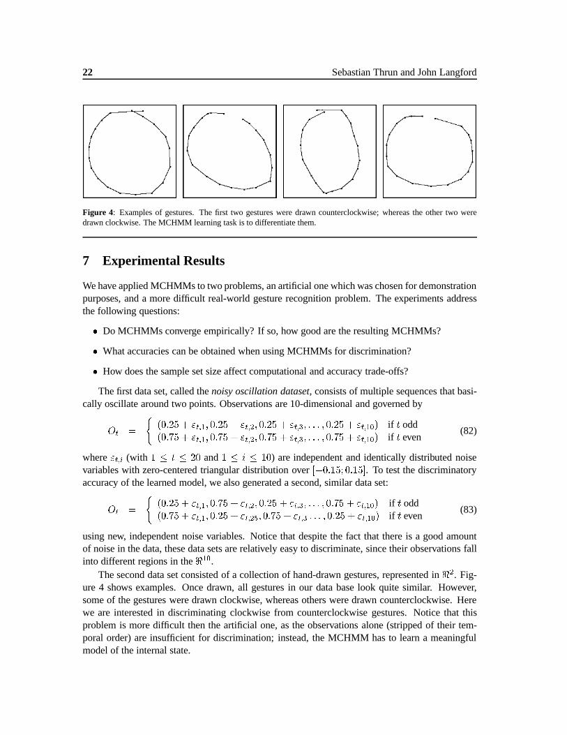
Figure 4: Examples of gestures. The first two gestures were drawn counterclockwise; whereas the other two weredrawn clockwise. The MCHMM learning task is to differentiate them.
7 Experimental Results
We have applied MCHMMs to two problems, an artificial one which was chosen for demonstrationpurposes, and a more difficult real-world gesture recognition problem. The experiments addressthe following questions:
� Do MCHMMs converge empirically? If so, how good are the resulting MCHMMs?
� What accuracies can be obtained when using MCHMMs for discrimination?
� How does the sample set size affect computational and accuracy trade-offs?
The first data set, called thenoisy oscillation dataset, consists of multiple sequences that basi-cally oscillate around two points. Observations are 10-dimensional and governed by
Ot =
((0:25 + "t;1; 0:25 + "t;2; 0:25 + "t;3; : : : ; 0:25 + "t;10) if t odd(0:75 + "t;1; 0:75 + "t;2; 0:75 + "t;3; : : : ; 0:75 + "t;10) if t even
(82)
where"t;i (with 1 � t � 20 and1 � i � 10) are independent and identically distributed noisevariables with zero-centered triangular distribution over[�0:15; 0:15]. To test the discriminatoryaccuracy of the learned model, we also generated a second, similar data set:
Ot =
((0:25 + "t;1; 0:75 + "t;2; 0:25 + "t;3; : : : ; 0:75 + "t;10) if t odd(0:75 + "t;1; 0:25 + "t;25; 0:75 + "t;3 : : : ; 0:25 + "t;10) if t even
(83)
using new, independent noise variables. Notice that despite the fact that there is a good amountof noise in the data, these data sets are relatively easy to discriminate, since their observations fallinto different regions in the<10.
The second data set consisted of a collection of hand-drawn gestures, represented in<2. Fig-ure 4 shows examples. Once drawn, all gestures in our data base look quite similar. However,some of the gestures were drawn clockwise, whereas others were drawn counterclockwise. Herewe are interested in discriminating clockwise from counterclockwise gestures. Notice that thisproblem is more difficult then the artificial one, as the observations alone (stripped of their tem-poral order) are insufficient for discrimination; instead, the MCHMM has to learn a meaningfulmodel of the internal state.

Monte Carlo Hidden Markov Models 23
2 4 6 8 10 12 14 16 18 20Iteration Baum-Welch
0
10
20
30
40
50
60
70
80
Lo
g s
core
of
trai
nin
g d
ata
2 4 6 8 10 12 14 16 18 20
0
10
20
30
40
50
60
70
80
Figure 5: Log score of training data as a function of the iteration of EM, for the synthetic data set. Top curve: 1000samples for all densities. Middle curve: 1000 samples for� and�, 100 samples for�, �, , and�. Bottom curve: 100samples for� and�, 10 samples for�, �, , and�. These graphs illustrate that MCHMMs tend to maximize the datalikelihood, even in the finite case. Each result is averaged over 10 independent experiments; 95% confidence bars arealso shown.
Figures 5 and 6 show results obtained for the first dataset. Shown in both figures are curvesthat characterize the “log score” as a function of the number of iterations. This score is the real-valued analogue to the likelihood; however, since densities can be larger than one, the score canalso be larger than one, and hence its logarithm is not bounded above.
The curves in Figure 5 show average log score for thetraining setas a function of the numberof iterations, averaged over 10 independent experiments (each curve). The different curves wereobtained using different numbers of samples which, contrary to the theoretical results, were keptconstant throughout the experiments:
Sample set sizeN for: : : �; � �; �; ; �
top curve: 1,000 1,000middle curve: 1,000 100bottom curve: 100 10
Figure 5 also provides 95% confidence bars for these results. The difference in absolute levels towhich the scores appear to converge stem from the fact that the maximum tree depth, and hencethe maximum of the tree densityf , is a function of the sample set size; hence, if the number ofsamples is small, the tree will remain shallow. The key observation, however, is their monotonicity.These curves demonstrate that each iteration in MCHMM indeed increases the data likelihood (orleaves it unchanged), even if only finitely many samples are used. This finding, which we alsoconsistently observed for other data sets and parameter settings, illustrate that MCHMMs arewell-behaved in practice, that is, the finiteness of the sample set appears not to cause catastrophicproblems.

24 Sebastian Thrun and John Langford
2 4 6 8 10 12 14 16 18 20Iteration Baum-Welch
-1
-2
0
1
2
3
4
5
6
7
8
Lo
g s
core
of
test
ing
dat
a
2 4 6 8 10 12 14 16 18 20
-1
-2
0
1
2
3
4
5
6
7
8
Figure 6: Log score of testing data as a function of the iteration of EM, for the synthetic data set. The top curve showsthe log score of data generated from the model used in training, whereas the bottom curve shows the log score for datagenerated from a different model. 95% confidence bars are also shown.
Figure 6 shows results for independent testing data. The upper curve in Figure 6 depicts the logscore for set of random sequence that are generated from the same model as the training sequences.The bottom curve depicts the log score for independently generated sequences using the othermodel, for which the MCHMM was not trained. In both cases, only a single data set (of length20) was used for training, and testing was performed using 20 data sets generated independently.N = 100 samples were used throughout for all densities�, �, , and�, andN = 1; 000 sampleswere used for� and�, to account for their higher dimensionality. The initial shrinkage factor was� = 1, which was annealed down at the rate�� = 0:9. In all experiments, the dimension of thestate space wask = 2. The results obtained for lower-dimensional observation spaces, which arenot shown here, were even better. In all cases, the score clearly reflected that the MCHMM hadlearned a good model. The classification accuracy for test sets was consistently 100%.
The result in Figure 6 illustrate the discriminative power of MCHMM for this data set. It alsodemonstrates the effect of annealing: The testing data likelihood is maximal at iteration 6 (thusthe optimal� is � = 0:53), beyond which the MCHMM starts overfitting the data. In our experi-ments, the optimal stopping point was consistently found within�1 step, using a single, indepen-dently generated sequence for cross-validation. In all our experiments, the MCHMM consistentlydiscriminated the two different classes without error, regardless of the settings of the individualparameters (we did not run experiments withN < 10). The bars in Figure 6 are confidence barsat the 95% confidence level.
Figure 7 shows the corresponding result for the more difficult gesture recognition problem.These results were obtained using a single gesture for training only, and using 50 gestures fortesting. The top curve depicts the log score for gestures drawn in the same direction as the traininggesture, whereas the bottom curve shows the log scores for gestures drawn in opposite direction.As easily noticed in Figure 7, the difference between classes is smaller than in Figure 6—which

Monte Carlo Hidden Markov Models 25
2 4 6 8 10 12 14 16 18 20 22 24 26Iteration Baum-Welch
0
1
2
3
Lo
g s
core
of
test
ing
dat
a
2 4 6 8 10 12 14 16 18 20 22 24 26
0
1
2
3
Figure 7: Log score for the gesture data base, obtained for independent testing data. The top curve shows the log scoreof gestures drawn in same same way as the training gesture, whereas the bottom curve shows the log score of gesturesdrawn in opposite direction.
comes at no surprise—, yet the score of the “correct” class is still a factor of 4 to 5 larger thanthat of the opposite class. Figure 7 also shows the effect of annealing. The best shrinkage valueis obtained after 12 iterations, where� = 0:28. As in the previous case, cross-validation using asingle gesture performs well. On average, the classification accuracy when using cross-validationfor early stopping is 86.0%. This rate is remarkably high, given that only a single gesture per classwas used for training.
A key advantage of MCHMM over HMMs lies in the ease of trading off computational com-plexity and accuracy. In conventional HMM, the computational complexity is fixed for any given(trained) model. In contrast, MCHMM permit variable sampling set sizes during run-time, afterthe model is trained. This leads to a niceany-timealgorithm [9, 58]. Once trained, a MCHMM cancontrol its computational complexity on-line by dynamically adjusting the sample size, dependingon the available resources. The any-time property is important for many real-world applications,where computation resources are bounded. To the best of our knowledge, the any-time nature is aunique property of MCHMMs, which is not shared by previous HMM algorithms.
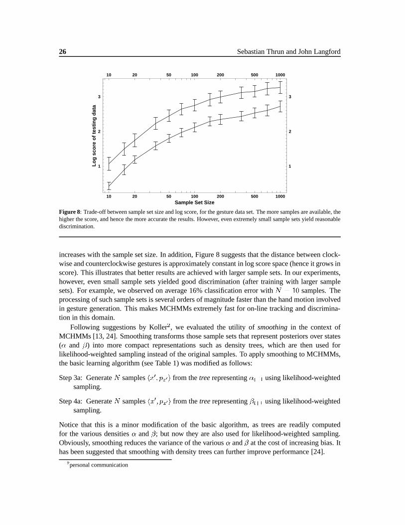
Figure 8 illustrates the trade-off between computation and accuracy empirically for the gesturedata base. Shown there is the trade-off between the number of samples and the likelihood of thetesting data. Notice that the horizontal axis is logarithmic. All of these points are generated usinga model� obtained using early stopping. The sample set size was generatedafter training, toinvestigate the effect of computational limitations on the on-line performance of the MCHMM.As in Figure 7, the top curve in Figure 8 depicts the log score of gestures drawn in the samedirection as the training data, whereas the bottom curve shows the log score of gestures drawn inopposite direction.
The result in Figure 8 illustrates that the score (and hence the accuracy) of both data sets in-creases with the sample set size. This is not surprising, as the accuracy of the approximations
26 Sebastian Thrun and John Langford
10 20 50 100 200 500 1000Sample Set Size
1
2
3L
og
sco
re o
f te
stin
g d
ata
10 20 50 100 200 500 1000
1
2
3
Figure 8: Trade-off between sample set size and log score, for the gesture data set. The more samples are available, thehigher the score, and hence the more accurate the results. However, even extremely small sample sets yield reasonablediscrimination.
increases with the sample set size. In addition, Figure 8 suggests that the distance between clock-wise and counterclockwise gestures is approximately constant in log score space (hence it grows inscore). This illustrates that better results are achieved with larger sample sets. In our experiments,however, even small sample sets yielded good discrimination (after training with larger samplesets). For example, we observed on average 16% classification error withN = 10 samples. Theprocessing of such sample sets is several orders of magnitude faster than the hand motion involvedin gesture generation. This makes MCHMMs extremely fast for on-line tracking and discrimina-tion in this domain.
Following suggestions by Koller2, we evaluated the utility ofsmoothingin the context ofMCHMMs [13, 24]. Smoothing transforms those sample sets that represent posteriors over states(� and �) into more compact representations such as density trees, which are then used forlikelihood-weighted sampling instead of the original samples. To apply smoothing to MCHMMs,the basic learning algorithm (see Table 1) was modified as follows:
Step 3a: GenerateN sampleshx0; px0i from thetreerepresenting�t�1 using likelihood-weightedsampling.
Step 4a: GenerateN sampleshx0; px0i from thetreerepresenting�t+1 using likelihood-weightedsampling.
Notice that this is a minor modification of the basic algorithm, as trees are readily computedfor the various densities� and�; but now they are also used for likelihood-weighted sampling.Obviously, smoothing reduces the variance of the various� and� at the cost of increasing bias. Ithas been suggested that smoothing with density trees can further improve performance [24].
2personal communication

Monte Carlo Hidden Markov Models 27
2 4 6 8 10 12 14 16 18 20 22 24 26Iteration Baum-Welch
0
1
2
3
Lo
g s
core
of
test
ing
dat
a
2 4 6 8 10 12 14 16 18 20 22 24 26
0
1
2
3
Figure 9: MCHMMs with (black curve) and without (grey curve) density tree smoothing of� and�, under otherwiseequal conditions. Each curve plots the log score of the testing data as a function of the number of Baum-Welch iterations.The grey curve is equivalent to the top curve in Figure 7. These results illustrate the negative effect of smoothing onlog score of the testing data.
Unfortunately, in our experiments we were unable to confirm the utility of smoothing in thecontext of MCHMMs. For the artificial data set, the generalization performance of MCHMMswith smoothing was indistinguishable from that obtained without smoothing, both in terms of logscore of the testing data and the class discrimination accuracy. Smoothing actually worsened theperformance for the gesture data set. Figure 9 shows the log score of testing data using smoothing(black curve), and compares it with the corresponding log scores obtained without smoothing(gray curve, copied from Figure 7). Smoothing was found to reduce the log score of the testingdata; thus, MCHMMs trained with smoothing are less capable of “explaining” new examples.This is not surprising, as smoothing is not an information loss-free operation, and it is not clearthat the inductive bias provided by a tree representation is beneficial. The reduction of the logscore led to a slight reduction of the discrimination accuracy. Using cross-validation, the averageclassification accuracy for MCHMMs with smoothing was 82.0%, which is 4.0% smaller than theaccuracy obtained without smoothing.
8 Related Work
Hidden Markov Models [2, 43] have been successfully applied to a huge range of applicationsrequiring temporal signal processing. As indicated in the introduction of this paper, most state-of-the-art speech recognition systems rely on HMMs (see, for example, the various papers in [54]).Recently, extensions of HMMs have been successfully applied in the context of mobile robotics[23, 48, 52], where they have led to improved solutions of theconcurrent mapping and localizationproblem, which is generally acknowledged as one of the most difficult problems in robotics [6, 25].

28 Sebastian Thrun and John Langford
These are just two examples of successful application areas of HMM; the number of successfulapplications is numerous.
Most HMM algorithms differ from MCHMMs in that they only apply to discrete state andobservation spaces. While the majority of HMM approaches represent states individually (in aflat way), some more recent approaches have extended HMMs to loosely coupled factorial repre-sentations [15, 46], which represent state by features but are nevertheless discrete. Others havesuccessfully proposed HMM models that can cope with real-valued observation spaces [29, 19].Our approach generalizes HMMs to continuous state and observation spaces with a large, non-parametric range of state transition and observation densities. It also differs from previous HMMapproaches in that it provides a mechanisms for complexity control (regularization); in previousapproaches, the complexity of the internal state space had to be calibrated carefully by hand. Fi-nally, MCHMMs provide a mechanisms to trade off computational requirements and accuracy inan any-time fashion, which differs from previous approaches whose computational requirementswere not adjustable during run-time [9, 58]. We envision that all of these advances are importantfor a broad range of practical problems.
Sampling techniques, one of the two methods used for density approximation in MCHMMs,have recently gained popularity in the applied statistics and AI literature. Various researchers haveapplied sampling methods in the context of state estimation in dynamical systems [3, 13, 22, 30,41] and learning [7]. A nice introduction into the use of sampling for density approximation can befound in [36]. Our approach to state estimation (computation of the�s) is essentially equivalentto the condensation algorithmproposed by Isard and Blake [18] and theMarkov localizationalgorithm proposed by Dellaert and colleagues [11, 10], both of which are basically versions ofthe well-knownsampling/importance resampling(SIR) algorithm [44, 49]. Similar approaches areknown asparticle filters[41], bootstrap[14], andsurvival of the fittest[22]. All these approachesare concerned with state estimation in an HMM-like or Kalman filter-like fashion. Thus, they relyon the a priori availability of� and�, which are learned from data by the MCHMM algorithmproposed here. To our knowledge, the application of sampling-based methods to learning non-parametric state transition models and observation models in HMMs is new, as is our proposal forthe integration of a forward (�) and backward (�) phase using trees. The theoretical results in thispaper demonstrate that our approach can be applied to a large class of problems, assuming thatsufficiently many samples are used. Trees have frequently been used for density approximation,most recently in [24, 35, 38, 39]. However, we are not aware of a proof of asymptotic consistencyfor density trees, although we suspect that such a result exists.
9 Conclusion
We have presented a new algorithm for hidden Markov models, called Monte Carlo HiddenMarkov Models (MCHMM). MCHMMs extend HMMs to real-valued state and observation spaces.They represent all densities by samples, which are transformed into probability density functionsusing density trees. Both representations were proven to be asymptotically consistent under mini-mal assumptions on the nature of the density that is being approximated. Because the continuousstate spaces are rich enough to fit (and over-fit) arbitrary data sets, our approach uses shrinkageto reduce its complexity. The shrinkage parameter is gradually annealed down over time, and
Monte Carlo Hidden Markov Models 29
cross-validation (early stopping) is used to select the best model complexity. The pervasive use ofMonte Carlo sampling led to the design of an any-time implementation, capable of dynamicallytrading off computational complexity and the accuracy of the results. Consequently, MCHMMsare well-suited for time-critical applications that are frequently encountered in the real world.
We have proved the asymptotic consistency of MCHMMs for a large class of probability den-sity functions. Empirical results, carried out in an artificial domain and a more challenging ges-ture recognition domain, demonstrate the our approach generalizes well even when trained withextremely scarce data. Additional experiments characterize the natural trade-off between sampleset size and accuracy, illustrating that good results may be achieved even from extremely smallsample sets.
While the theoretical results of this paper hold only in the limit, actual applications have to livewith finite sample sets. Thus, an interesting and open question is under what conditions MCHMMwith finite sample sets converges, and what error to expect. While principal error bounds of thistype are relatively easy to obtain in static approximation setting, the recursive nature of Baum-Welch makes it difficult to obtain bounds for MCHMM. The empirical results described here,however, suggest that MCHMM is a robust method that works well in practice even with relativelysmall sample sets.
We conjecture that MCHMMs are better suited for many real-world application domains suchas speech and robotics applications than conventional HMMs, for primarily three reasons: theirsupport of continuous representations of observations and state, their built-in mechanisms formodel selection, which reduces the burden of picking the “right” model (e.g., number of statesin conventional HMMs), and, finally, their support of any-time computation, which makes themextremely compliant in time-critical applications with bounded computational resources.
Acknowledgement
The authors gratefully acknowledge inspiring discussions with Frank Dellaert, Nir Friedman, Di-eter Fox, Daphne Koller, and Larry Wasserman.
References
[1] P. Baldi and Y. Chauvin. Smooth online learning algorithms for hidden Markov models.Neural Computation, 6:307–318, 1994.
[2] L.E. Baum and T. Petrie. Statistical inference for probabilistic functions of finite state markovchains.Annals of Mathematical Statistics, 37:1554–1563, 1966.
[3] X. Boyen and D. Koller. Tractable inference for complex stochastic processes. InProceed-ings of Uncertainty in Artificial Intelligence, pages 33–42, Madison, WI, 1998.
[4] W. Burgard, A.B. Cremers, D. Fox, D. H¨ahnel, G. Lakemeyer, D. Schulz, W. Steiner, andS. Thrun. Experiences with an interactive museum tour-guide robot. Technical ReportCMU-CS-98-139, Carnegie Mellon University, Computer Science Department, Pittsburgh,PA, 1998.

30 Sebastian Thrun and John Langford
[5] E. Charniak.Statistical Language Learning. MIT Press, Cambridge, Massachusetts, 1993.
[6] I.J. Cox. Blanche—an experiment in guidance and navigation of an autonomous robot vehi-cle. IEEE Transactions on Robotics and Automation, 7(2):193–204, 1991.
[7] J.F.G. de Freitas, S.E. Johnson, M. Niranjan, and A.H. Gee. Global optimisation of neuralnetwork models via sequential sampling-importance resampling. InProceedings of the In-ternational Conference on Spoken Language Processing (ICSLP), Sydney, Australia, 1998.
[8] T. Dean and K. Kanazawa. A model for reasoning about persistence and causation.Compu-tational Intelligence, 5(3):142–150, 1989.
[9] T. L. Dean and M. Boddy. An analysis of time-dependent planning. InProceeding of Sev-enth National Conference on Artificial Intelligence AAAI-92, pages 49–54, Menlo Park, CA,1988. AAAI, AAAI Press/The MIT Press.
[10] F. Dellaert, W. Burgard, D. Fox, and S. Thrun. Using the condensation algorithm for robust,vision-based mobile robot localization. Submitted for publication, 1998.
[11] F. Dellaert, D. Fox, W. Burgard, and S. Thrun. Monte carlo localization for mobile robots.Submitted for publication, 1998.
[12] A.P. Dempster, A.N. Laird, and D.B. Rubin. Maximum likelihood from incomplete data viathe em algorithm.Journal of the Royal Statistical Society, Series B, 39(1):1–38, 1977.
[13] A Doucet. On sequential simulation-based methods for bayesian filtering. Technical ReportCUED/F-INFENG/TR 310, Cambridge University, Department of Engineering, Cambridge,UK, 1998.
[14] B. Efron and R.J. Tibshirani.An Introduction to the Bootstrap. Chapman & Hall, New York,1993.
[15] Z. Ghahramani and M.I. Jordan. Factorial hidden markov models. InAdvances in Neu-ral Information Processing Systems 8 (NIPS), pages 472–478, Cambridge, MA, 1996. MITPress.
[16] B. Hannaford and P. Lee. Hidden markov model analysis of force torque information intelemanipulation.International Journal of Robotics Research, 10(5):528–539, 1991.
[17] J. Henderson, S. Salzberg, and K. Fasman. Finding genes in human DNA with a hiddenMarkov model. InProceedings of Intelligent Systems for Molecular Biology ’96, WashingtonUniversity, St. Louis, MI, 1996.
[18] M. Isard and A. Blake. Condensation: conditional density propagation for visual tracking.International Journal of Computer Vision, in press 1998.
[19] B.H. Juang. Maximum likelihood estimation for mixture multivariate stochastic observationsof markov chains.AT&T Technical Journal, 64(6), 1985.

Monte Carlo Hidden Markov Models 31
[20] B.H. Juang, S.E. Levinson, and M.M. Sondhi. Maximum likelihood estimation for multi-variate mixture observations of markov chains.IEEE Transaction and Information Theory,32(2), 1986.
[21] R. E. Kalman. A new approach to linear filtering and prediction problems.Trans. ASME,Journal of Basic Engineering, 82:35–45, 1960.
[22] K. Kanazawa, D. Koller, and S.J. Russell. Stochastic simulation algorithms for dynamicprobabilistic networks. InProceedings of the 11th Annual Conference on Uncertainty in AI,Montreal, Canada, 1995.
[23] S. Koenig and R. Simmons. Passive distance learning for robot navigation. In L. Saitta,editor,Proceedings of the Thirteenth International Conference on Machine Learning, 1996.
[24] D. Koller and R. Fratkina. Using learning for approximation in stochastic processes. InProceedings of the International Conference on Machine Learning (ICML), 1998.
[25] D. Kortenkamp, R.P. Bonasso, and R. Murphy, editors.AI-based Mobile Robots: Casestudies of successful robot systems, Cambridge, MA, 1998. MIT Press.
[26] A. Krogh, I.S. Mian, and D. Haussler. A hidden markov model that finds genes in e. colidna.Nucleic Acids Research, 22:476–8–4778, 1994.
[27] K.-F. Lee.Automatic Speech Recognition: The Development of the SPHINX System. KluwerPublishers, Boston, MA, 1989.
[28] K.-F. Lee. Context-dependent phonetic hidden markov models for speaker-independent con-tinuous speech recognition. In A. Waibel and K.-F. Lee, editors,Readings in Speech Recog-nition. Morgan Kaufmann Publishers, Inc., San Mateo, CA, 1990. Also appeared in the IEEETransactions on Acoustics, Speech, and Signal Processing.
[29] L.A. Liporace. Maximum likelihood estimation for multivariate observations of markovsources.IEEE Transactions in Information Theory, 28(5), 1982.
[30] J. Liu and R. Chen. Sequential monte carlo methods for dynamic systems.Journal of theAmerican Statistical Association, 93, 1998.
[31] P. Maybeck.Stochastic Models, Estimation, and Control, Volume 1. Academic Press, Inc,1979.
[32] A. McCallum, R. Rosenfeld, T. Mitchell, and A.Y. Ng. Improving text classification byshrinkage in a hierarchy of classes. InProceedings of the International Conference on Ma-chine Learning (ICML), 1998.
[33] G.J. McLachlan and T. Krishnan.The EM Algorithm and Extensions. Wiley Series in Prob-ability and Statistics, New York, 1997.
[34] M. Meila and M.I. Jordan. Learning fine motion by markov mixture of experts. InAdvancesin Neural Information Processing Systems 8 (NIPS), pages 1003–1009, Cambridge, MA,1996. MIT Press.

32 Sebastian Thrun and John Langford
[35] A.W. Moore, J. Schneider, and K. Deng. Efficient locally weighted polynomial regressionpredictions. InProceedings of the International Conference on Machine Learning. MorganKaufmann Publishers, 1997.
[36] R.M. Neal. Probabilistic inference using markov chain monte carlo methods. Technical Re-port CRG-TR-93-1, Dept. of Computer Science, University of Toronto, Toronto, CA, 1993.
[37] R.M. Neal and G.E. Hinton. A view of the EM algorithm that justifies incremental, sparse,and other variants. In M.I. Jordan, editor,Learning in Graphical Models. Kluwer AcademicPress, 1998.
[38] S. M. Omohundro. Efficient Algorithms with Neural Network Behavior.Journal of ComplexSystems, 1(2):273–347, 1987.
[39] S. M. Omohundro. Bumptrees for Efficient Function, Constraint, and Classification Learn-ing. In R. P. Lippmann, J. E. Moody, and D. S. Touretzky, editors,Advances in NeuralInformation Processing Systems 3. Morgan Kaufmann, 1991.
[40] A.G. Pedersen, P. Baldi, S. Brunak, and Y. Chauvin. Characterization of prokaryotic andeukaryotic promoters using hidden markov models. InProceedings of Intelligent Systemsfor Molecular Biology ’96, Washington University, St. Louis, MI, 1996.
[41] M. Pitt and N. Shephard. Filtering via simulation: auxiliary particle filter.Journal of theAmerican Statistical Association, 1999. Forthcoming.
[42] L. R. Rabiner. A tutorial on hidden markov models and selected applications in speechrecognition. InProceedings of the IEEE. IEEE, 1989. IEEE Log Number 8825949.
[43] L.R. Rabiner and B.H. Juang. An introduction to hidden markov models. InIEEE ASSPMagazine, 1986.
[44] D.B. Rubin. Using the SIR algorithm to simulate posterior distributions. In M.H. Bernardo,K.M. an DeGroot, D.V. Lindley, and A.F.M. Smith, editors,Bayesian Statistics 3. OxfordUniversity Press, Oxford, UK, 1988.
[45] S. Russell and P. Norvig.Artificial Intelligence: A Modern Approach. Prentice Hall, Engle-wood Cliffs, NJ, 1995.
[46] L.K. Saul and M.I. Jordan. Exploiting tractable substructures in intractable networks. InAdvances in Neural Information Processing Systems 8 (NIPS), pages 486–492, Cambridge,MA, 1996. MIT Press.
[47] H. Shatkay.Learning Models for Robot Navigation. PhD thesis, Computer Science Depart-ment, Brown University, Providence, RI, 1998.
[48] H Shatkay and L. Kaelbling. Learning topological maps with weak local odometric infor-mation. InProceedings of IJCAI-97. IJCAI, Inc., 1997.

Monte Carlo Hidden Markov Models 33
[49] A.F.M. Smith and A.E. Gelfand. Bayesian statistics without tears: a sampling-resamplingperspective.American Statistician, 46:84–88, 1992.
[50] C. Stein. Inadmissibility of the usual estimator for the mean of a multivariate normal dis-tribution. In Proceedings of the Third Berkeley Symposium on Mathematical Statistics andProbability 1, pages 197–206. University of California Press, 1955.
[51] M.A. Tanner.Tools for Statistical Inference. Springer Verlag, New York, 1993. 2nd edition.
[52] S. Thrun, D. Fox, and W. Burgard. A probabilistic approach to concurrent mapping and local-ization for mobile robots.Machine Learning, 31:29–53, 1998. also appeared in AutonomousRobots 5, 253–271.
[53] V. Vapnik. Estimations of dependences based on statistical data. Springer Publisher, 1982.
[54] A. Waibel and K.-F. Lee, editors.Readings in Speech Recognition. Morgan KaufmannPublishers, San Mateo, Californien, 1990.
[55] A. S. Weigend and N. A. Gershenfeld, editors.Time Series Prediction. Addison-Wesley,Reading, MA, September 1993.
[56] G. Welch and G. Bishop. An introduction to the kalman filter. Technical Report TR 95-041,University of North Carolina, Department of Computer Science, 1995.
[57] G. Winkler. Image Analysis, Random Fields, and Dynamic Monte Carlo Methods. SpringerVerlag, Berlin, 1995.
[58] S. Zilberstein and S. Russell. Approximate reasoning using anytime algorithms. In S. Natara-jan, editor, Imprecise and Approximate Computation. Kluwer Academic Publishers, Dor-drecht, 1995.