Monte Carlo

Methods in Forecasting the Demand

for Electricity

Frank S. McGowanMarket Forecast

DepartmentOctober 26, 2007

2

Contents

•BC Hydro

•Load Forecasting at BC Hydro

•Stochastic Forecasting

• Monte Carlo Simulation

•BC Hydro’s Monte Carlo Model

•Model Results

• Description of the Model

•Comparison with Other Methods

•Conclusion

3

4

BC Hydro

• BC Hydro is the major provider of electricity in the province of British Columbia. • It is one of the largest electric utilities in Canada• 1.7 million customers in an area containing over 94 per cent of BC's population.

(4,364,565 in 2007).• Generating capacity over 11,000 megawatts (MW)• 90.3% from hydroelectric sources .• BC Hydro's various facilities generate between 43,000 and 54,000 gigawatt hours of

electricity annually, depending on prevailing water levels. • For fiscal 2006, domestic electric sales volume reached 52,440 gigawatt hours. and

52,911 for fiscal 2007.• Net income was $266 million In fiscal 2006, $407 million in fiscal 2007. • Employees 4,546 in March 2007 - Including its subsidiaries and British Columbia

Transmission Corporation. • New Energy – Green Emphasis

> Independent Power Producers > Site-C

5

Load Forecasting at BCHydro

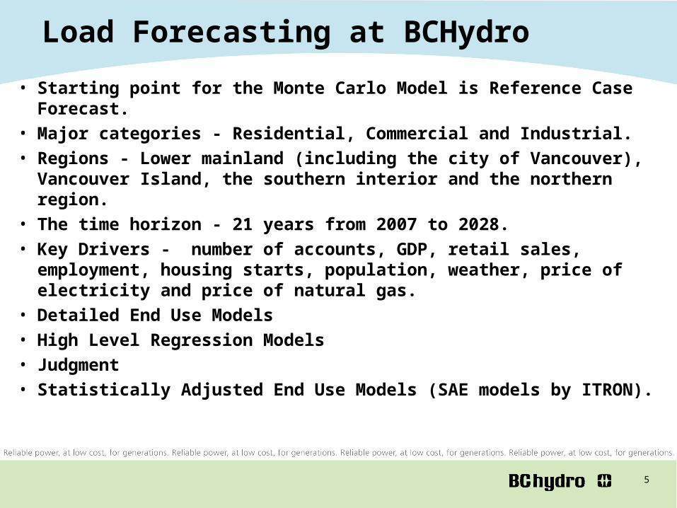
• Starting point for the Monte Carlo Model is Reference Case Forecast.• Major categories - Residential, Commercial and Industrial. • Regions - Lower mainland (including the city of Vancouver), Vancouver

Island, the southern interior and the northern region. • The time horizon - 21 years from 2007 to 2028.• Key Drivers - number of accounts, GDP, retail sales, employment,

housing starts, population, weather, price of electricity and price of natural gas.

• Detailed End Use Models• High Level Regression Models• Judgment• Statistically Adjusted End Use Models (SAE models by ITRON).

6

Stochastic Forecasting

• The Future is Uncertain. A deterministic forecast provides an incomplete picture. The appropriate model is a stochastic process.

• Definition (informal) : A stochastic process is a collection of random variables X together with their probability distributions which are indexed by time.

{ F( X, t ) }

7

Stochastic Forecasting

• Let y(t) and xj(t) (j=1,…k) be random variables defined by stochastic processes.

• Suppose there is a model that relates these variables. y(t) = L (x1(t), x2(t), …, xk(t) ) • If the probability distributions of the independent variables are

known, then the model specifies the probability distribution of y(t).• But it would usually be very difficult to work out this distribution

analytically.• Monte Carlo Simulation allows us to bypass this difficulty. @RISK

facilitates these simulations.

8

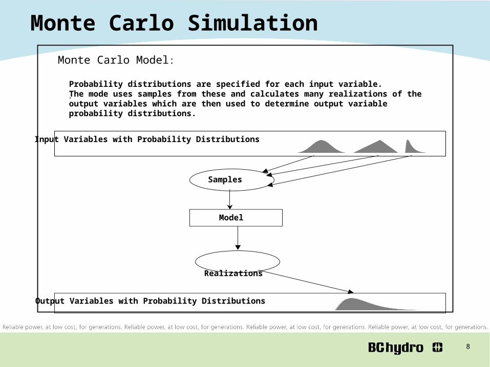
Monte Carlo MethodsMonte Carlo Model:

Probability distributions are specified for each input variable. The mode uses samples from these and calculates many realizations of the output variables which are then used to determine output variable probability distributions..

Input Variables with Probability Distributions

Output Variables with Probability Distributions

Model

Realizations

Samples

Monte Carlo Simulation

9

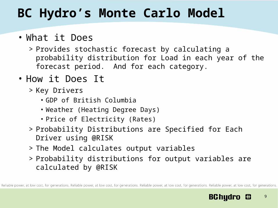
BC Hydro’s Monte Carlo Model

• What it Does> Provides stochastic forecast by calculating a probability distribution

for Load in each year of the forecast period. And for each category.

• How it Does It> Key Drivers

• GDP of British Columbia• Weather (Heating Degree Days)• Price of Electricity (Rates)

> Probability Distributions are Specified for Each Driver using @RISK> The Model calculates output variables> Probability distributions for output variables are calculated by @RISK

10

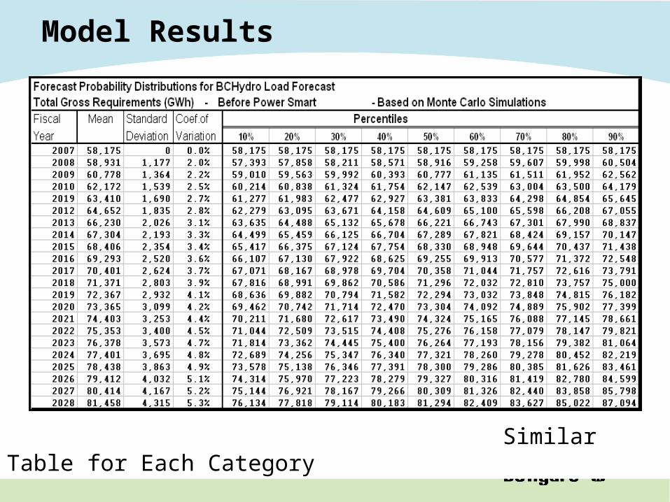
Model Results

Similar Table for Each Category

11

12

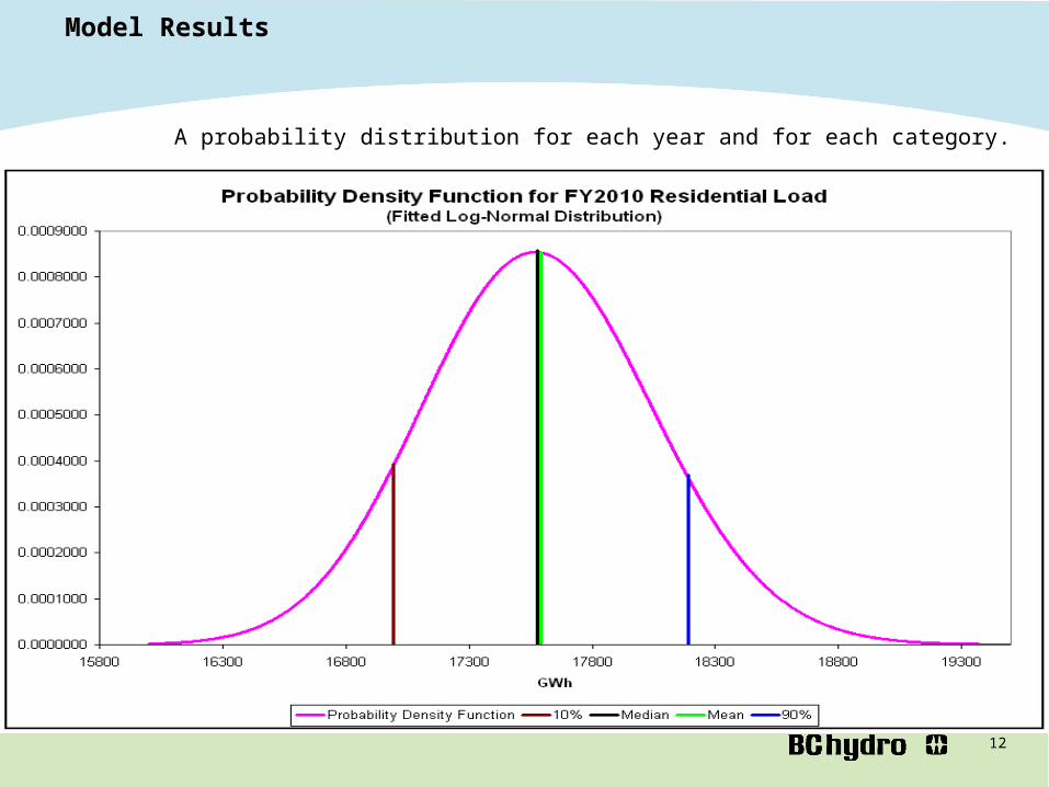
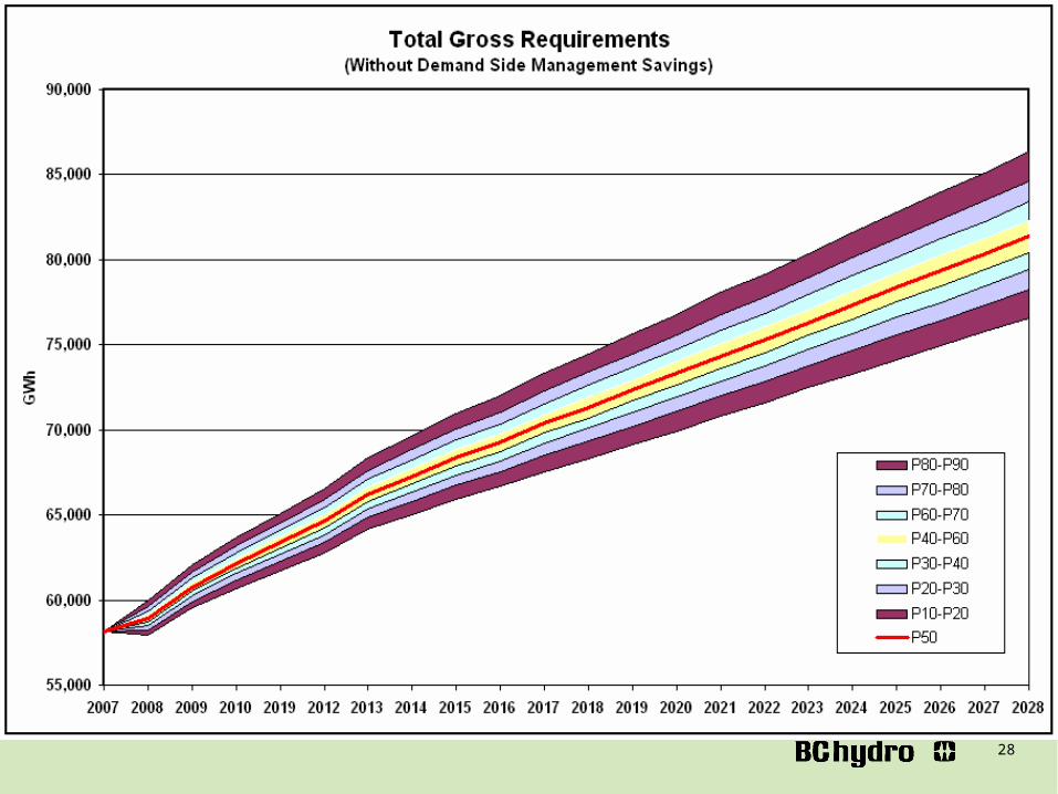
Model Results

A probability distribution for each year and for each category.

13

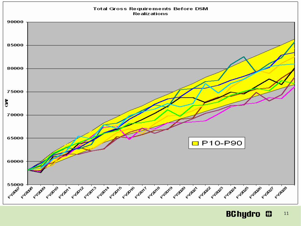
Model Results

Width of Distributions Increases With Time

14

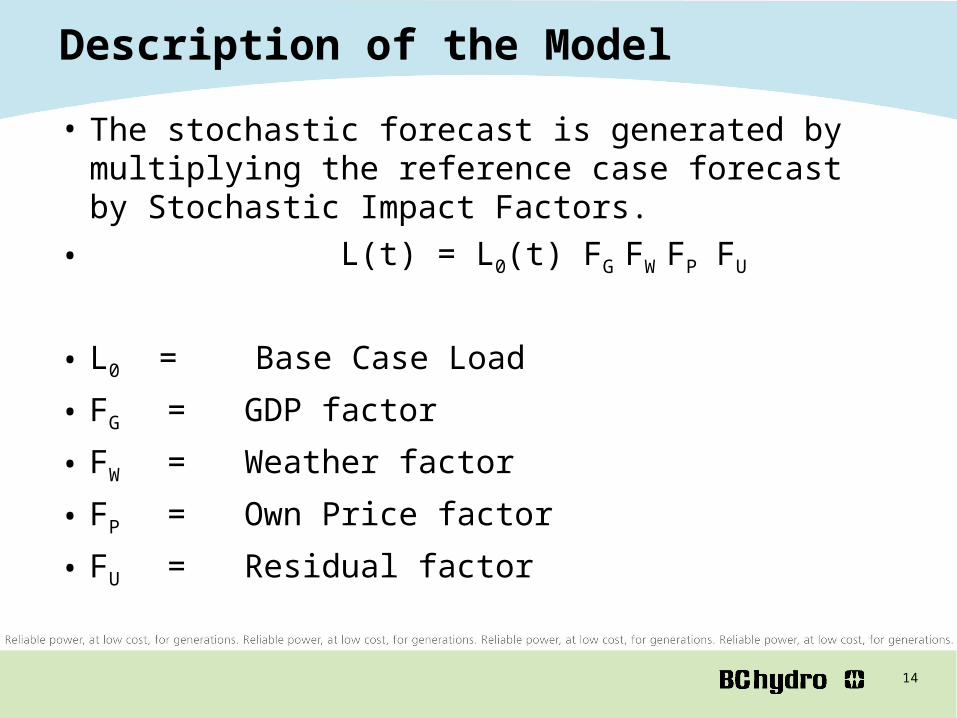
Description of the Model

• The stochastic forecast is generated by multiplying the reference case forecast by Stochastic Impact Factors.

• L(t) = L0(t) FG FW FP FU

• L0 = Base Case Load

• FG = GDP factor

• FW = Weather factor

• FP = Own Price factor

• FU = Residual factor

15

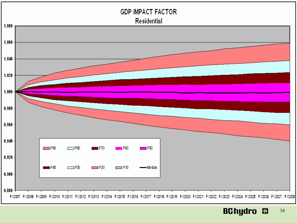
GDP Impact Factor

• Gt - GDP at time t.

• 0Gt - Reference case GDP forecast (from CFB Canada).

• gt - growth rate of reference case forecast. • Perturbed GDP forecast grows by the equation:

Gt = Gt-1 ( 1 + gt + ut )

• ut - perturbation that is N(0,) with = 1.54% • FG the GDP impact factor is given by:

FG = exp[ ln(Gt / 0Gt ) ] = ( Gt / 0Gt ) where:

is the elasticity of Load with respect to GDP.

16

17

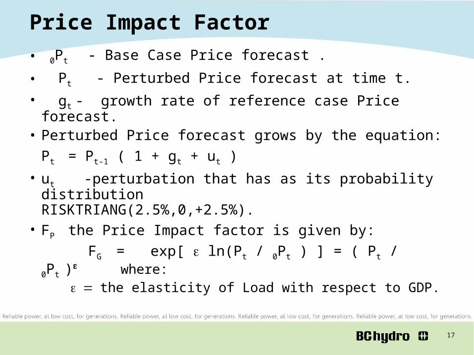
Price Impact Factor

• 0Pt - Base Case Price forecast .

• Pt - Perturbed Price forecast at time t.• gt - growth rate of reference case Price forecast. • Perturbed Price forecast grows by the equation:

Pt = Pt-1 ( 1 + gt + ut ) • ut -perturbation that has as its probability distribution

RISKTRIANG(2.5%,0,+2.5%).• FP the Price Impact factor is given by: FG = exp[ ln(Pt / 0Pt ) ] = ( Pt / 0Pt ) where:

the elasticity of Load with respect to GDP.

18

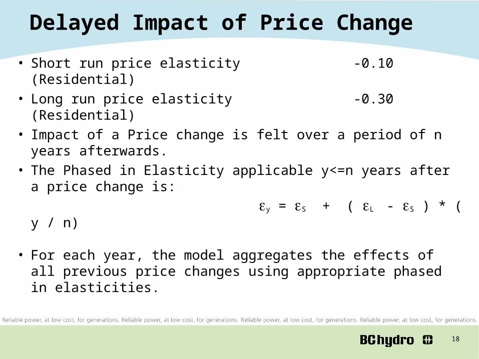
Delayed Impact of Price Change

• Short run price elasticity -0.10 (Residential)• Long run price elasticity -0.30 (Residential)• Impact of a Price change is felt over a period of n years afterwards.• The Phased in Elasticity applicable y<=n years after a price change

is: y = S + ( L - S ) * ( y / n)

• For each year, the model aggregates the effects of all previous price changes using appropriate phased in elasticities.

19

Price Change Scenarios

• Different price change scenarios can specified by choosing the reference case growth rate gt .

• Probability distributions are then calculated around whatever scenario is used as a reference case.

20

21

22

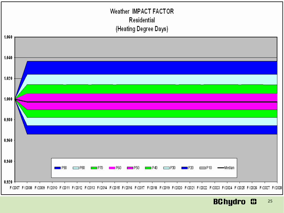
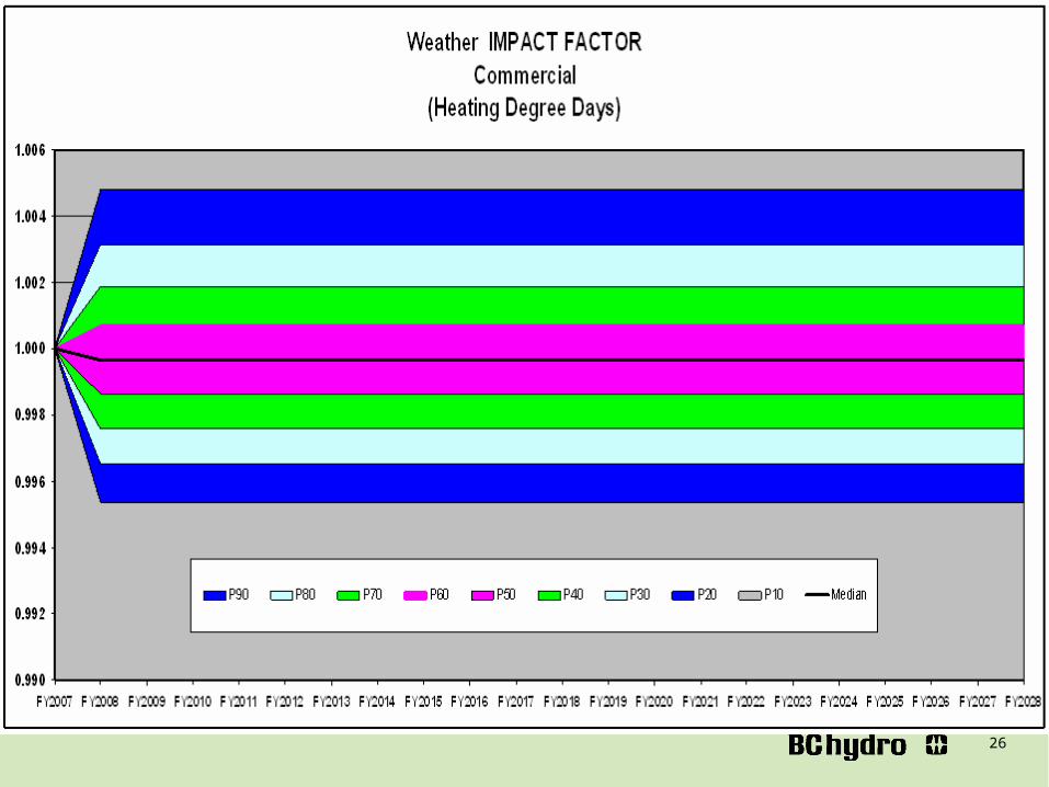
Weather Impact Factor

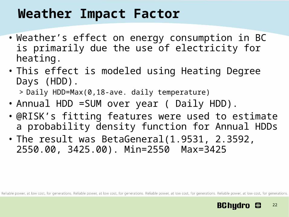
• Weather’s effect on energy consumption in BC is primarily due the use of electricity for heating.

• This effect is modeled using Heating Degree Days (HDD).> Daily HDD=Max(0,18-ave. daily temperature)

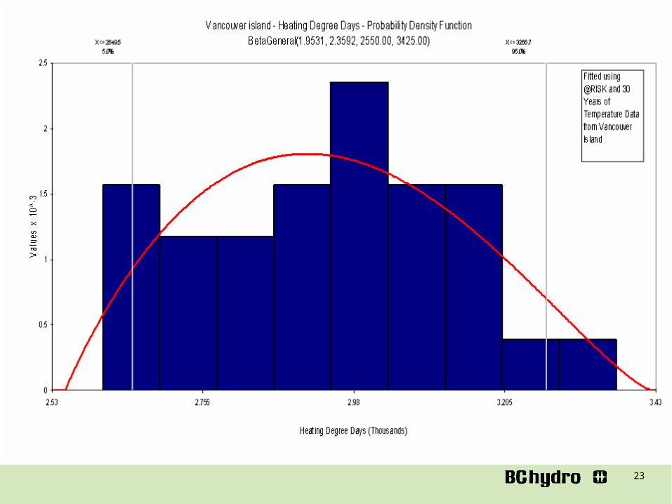
• Annual HDD =SUM over year ( Daily HDD). • @RISK’s fitting features were used to estimate a probability

density function for Annual HDDs• The result was BetaGeneral(1.9531, 2.3592, 2550.00,

3425.00). Min=2550 Max=3425

23

24

Weather Impact Factor

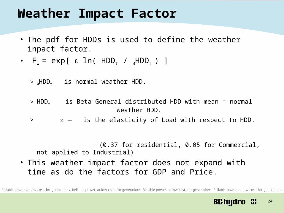
• The pdf for HDDs is used to define the weather inpact factor.• Fw = exp[ ln( HDDt / 0HDDt ) ]

> 0HDDt is normal weather HDD.

> HDDt is Beta General distributed HDD with mean = normal weather HDD.

> is the elasticity of Load with respect to HDD.

(0.37 for residential, 0.05 for Commercial, not applied to Industrial)

• This weather impact factor does not expand with time as do the factors for GDP and Price.

25

26

27

Demand Side Management and Residual

•0DSM(t) = Reference case forecast of DSM savings.

• The Monte Carlo Model gives these savings the following probability density function:

DSM(t) = RiskTriang(75%,100%,125%)*0DSM(t) then load after DSM is calculated by subtraction.

LOADafter(t) = LOADbefore(t) – DSM(t)• The residual impact factor is :

FU (t) = FU (t-1) * (1 + RiskTriang(-0.2%,0.0%,0.2%) )

28

29

Comparison With Other Methods

• Standard Linear Regression Model

• y = X + u• where: y is vector of data for dependent variable (Nx1).

X data matrix for independent variables (Nxk).

u is normal with zero mean and st. dev (Nx1). • In the Estimation Period X is non-stochastic and there are N data points.• Estimator of is b = (X’X)-1X’y = + (X’X)-1X’u • b is normally distributed because u is.• Estimator of y is ŷ = X b

30

Regression Model and Monte Carlo Compared

• A regression of Sales on GDP was estimated by OLS.• The results are graphed on the next slide.• BC Hydro’s Base Case Forecast is shown for

comparison.

31

Regression Model Predicts Sales Well

32

Forecasting Using Regression Model

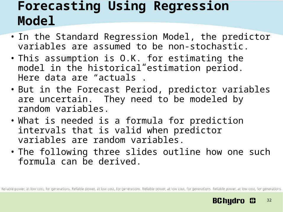
• In the Standard Regression Model, the predictor variables are assumed to be non-stochastic.

• This assumption is O.K. for estimating the model in the historical estimation period. Here data are “actuals”.

• But in the Forecast Period, predictor variables are uncertain. They need to be modeled by random variables.

• What is needed is a formula for prediction intervals that is valid when predictor variables are random variables.

• The following three slides outline how one such formula can be derived.

33

Forecasting Using Regression Model

• In Forecasting Period (t=1,…,T):• Predictor Variables X are Stochastic. • Let X = Z + V where Z = E[X], the mean of X.• The model is y = Z + u = Z + (V + u).• Assume that Z is a matrix of given non-stochastic forecasts

of the predictor variables and • V is modeled so that Vt j ~ N(0, t j ) and • Predictor variables and the error term { V, u } are a set of

independent random variables.> That is, Vt j and Vs k and uare all independent unless

indices t = and j = k.

34

Forecasting Using Regression Model

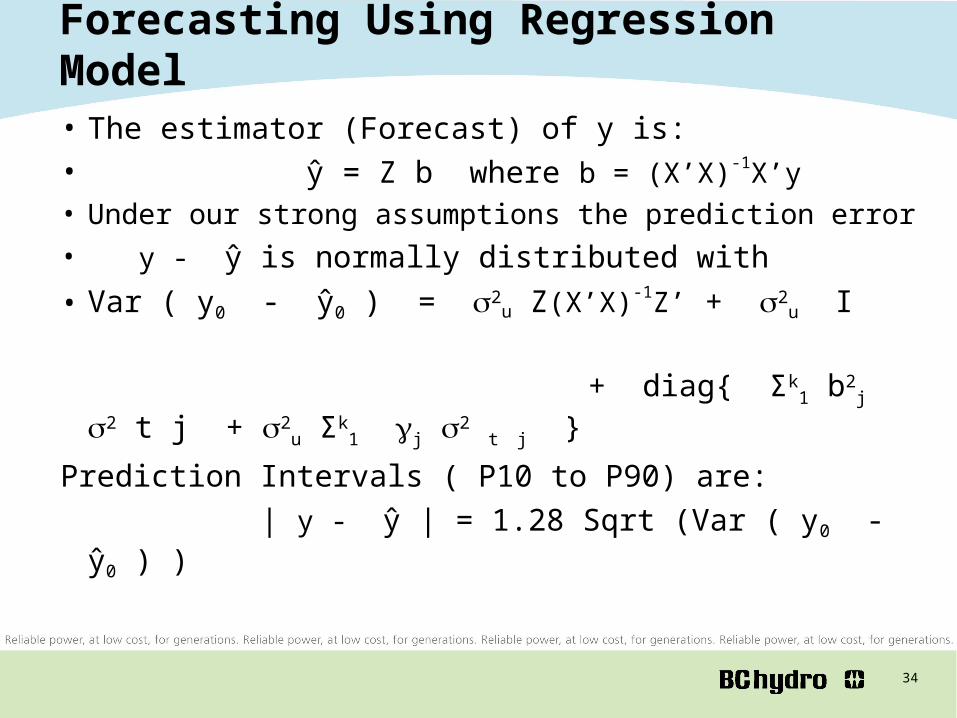
• The estimator (Forecast) of y is:• ŷ = Z b where b = (X’X)-1X’y • Under our strong assumptions the prediction error• y - ŷ is normally distributed with • Var ( y0 - ŷ0 ) = 2

u Z(X’X)-1Z’ + 2u I

+ diag{ Σk

1 b2j 2 t j + 2

u Σk1 j 2 t j }

Prediction Intervals ( P10 to P90) are: | y - ŷ | = 1.28 Sqrt (Var ( y0 - ŷ0 ) )

35

Forecasting Using Regression Model

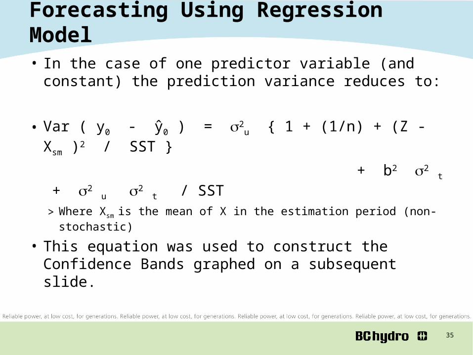
• In the case of one predictor variable (and constant) the prediction variance reduces to:

• Var ( y0 - ŷ0 ) = 2u { 1 + (1/n) + (Z - Xsm )2 / SST }

+ b2 2 t + 2 u 2 t / SST> Where Xsm is the mean of X in the estimation period (non-stochastic)

• This equation was used to construct the Confidence Bands graphed on a subsequent slide.

36

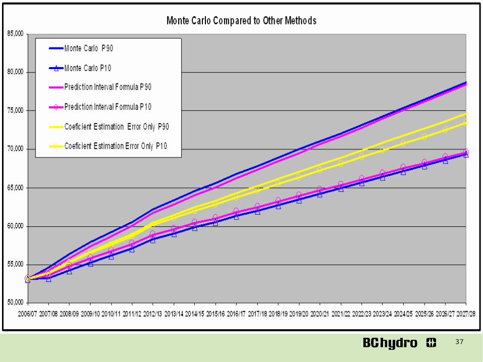
Comparison of Confidence Bands

• Confidence Bands were also produced by the Monte Carlo methodology explained previously.

• A third set of Confidence Bands was produced using only the first 3 terms of the prediction variance equation. These bands are due to coefficient estimation and residual error only.

• Note that:> The Monte Carlo and Prediction Formula Bands are Very Close.> The third set of bands are small compared to the others, showing that

uncertainty in the predictor variables in the forecast period is the main source of error in forecasted Load.

• This is true for a “good” regression, like the one considered here, where in the prediction interval formula, SST is large compared to the other terms.

37

38

39

Conclusion

• BC Hydro’s Monte Carlo Model and its implementation using @RISK was described.

• It provides a method for generating a stochastic forecast of the various components of BC Hydro’s Load.

• The results are reasonably accurate and have survived regulatory scrutiny for several years.

• Confidence bands resulting from the Monte Carlo Model and from an econometric prediction interval formula were calculated and compare. They are close to each other.