monte carlo search - paris dauphine university
TRANSCRIPT


Outline
• Monte Carlo Tree Search
• Nested Monte Carlo Search
• Nested Rollout Policy Adaptation
• Playout Policy Adaptation
• Zero Learning (Deep RL)
• Imperfect Information Games


Monte Carlo Tree Search

Monte Carlo Go
• 1993 : first Monte Carlo Go program– Gobble, Bernd Bruegmann.– How nature would play Go ?– Simulated annealing on two lists of moves.– Statistics on moves.– Only one rule : do not fill eyes.– Result = average program for 9x9 Go.– Advantage : much more simple than alternative
approaches.

Monte Carlo Go
• 1998 : first master course on Monte Carlo Go.
• 2000 : sampling based algorithm instead of simulated annealing.
• 2001 : Computer Go an AI Oriented Survey.
• 2002 : Bernard Helmstetter.
• 2003 : Bernard Helmstetter, Bruno Bouzy, Developments on Monte Carlo Go.
Monte Carlo Phantom Go
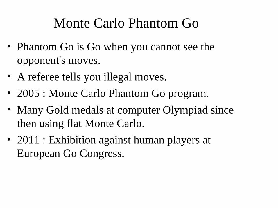
• Phantom Go is Go when you cannot see the opponent's moves.
• A referee tells you illegal moves.
• 2005 : Monte Carlo Phantom Go program.
• Many Gold medals at computer Olympiad since then using flat Monte Carlo.
• 2011 : Exhibition against human players at European Go Congress.

UCT
• UCT : Exploration/Exploitation dilemma for trees
[Kocsis and Szepesvari 2006].
• Play random random games (playouts).
• Exploitation : choose the move that maximizes the mean of the playouts starting with the move.
• Exploration : add a regret term (UCB).

• UCT : exploration/exploitation dilemma.• Play the move that maximizes
UCT

UCT

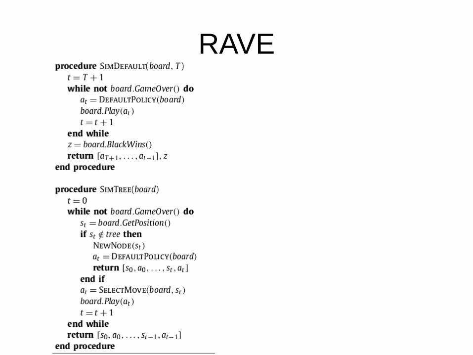
RAVE
● A big improvement for Go, Hex and other games is Rapid Action Value Estimation (RAVE) [Gelly and Silver 2007].
● RAVE combines the mean of the playouts that start with the move and the mean of the playouts that contain the move (AMAF).

RAVE● Parameter βm for move m is :
βm←pAMAFm / (pAMAFm + pm + bias × pAMAFm× pm)
● βm starts at 1 when no playouts and decreases as more playouts are played.
● Selection of moves in the tree :
argmaxm((1.0 − βm) × meanm + βm × AMAFm)
GRAVE
● Generalized Rapid Action Value Estimation (GRAVE) is a simple modification of RAVE.
● It consists in using the first ancestor node with more than n playouts to compute the RAVE values.
● It is a big improvement over RAVE for Go, Atarigo, Knightthrough and Domineering [Cazenave 2015].
Atarigo

Knightthrough

Domineering

Go

RAVE vs UCT
Game Score
Atarigo 8x8 94.2 %
Domineering 72.6 %
Go 9x9 73.2 %
Knightthrough 56.2 %
Three Color Go 9x9 70.8 %

GRAVE vs RAVE
Game Score
Atarigo 8x8 88.4 %
Domineering 62.4 %
Go 9x9 54.4 %
Knightthrough 67.2 %
Three Color Go 9x9 57.2 %

Parallelization of MCTS
• Root Parallelization.
• Tree Parallelization (virtual loss).
• Leaf Parallelization.

MCTS
• Great success for the game of Go since 2007.
• Much better than all previous approaches to computer Go.
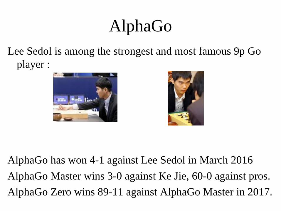
AlphaGoLee Sedol is among the strongest and most famous 9p Go
player :
AlphaGo has won 4-1 against Lee Sedol in March 2016
AlphaGo Master wins 3-0 against Ke Jie, 60-0 against pros.
AlphaGo Zero wins 89-11 against AlphaGo Master in 2017.

General Game Playing
• General Game Playing = play a new game just given the rules.
• Competition organized every year by Stanford.
• Ary world champion in 2009 and 2010.
• All world champions since 2007 use MCTS.

General Game Playing
• Eric Piette combined Stochastic Constraint Programming with Monte Carlo in WoodStock.
• World champion in 2016 (MAC-UCB-SYM).
• Detection of symmetries in the states.

Other two-player games
• Hex : 2009
• Amazons : 2009
• Lines of Action : 2009

MCTS Solver
● When a subtree has been completely explored the exact result is known.
● MCTS can solve games.● Score Bounded MCTS is the extension of
pruning to solving games with multiple outcomes.
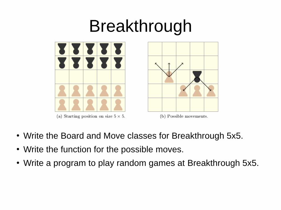
Breakthrough
● Write the Board and Move classes for Breakthrough 5x5.● Write the function for the possible moves.● Write a program to play random games at Breakthrough 5x5.
• Write, in the Board class, a score function to score a game (1.0 if White wins, 0.0 else) and a terminal function to detect the end of the game.
• Write, in the Board class, a playout function that plays a random game from the current state and returns the result of the random game.
Playouts

• Keep statistics for all the moves of the current state.
• For each move of the current state, keep the number of playouts starting with the move and the number of playouts starting with the move that have been won.
• Play the move with the greatest mean when all the playouts are finished.
Flat Monte Carlo

Choose the first move at the root according to UCB before each playout:
UCB

• Make UCB with 1 000 playouts play 100 games against Flat with 1 000 playouts.
• Winrate ?
• Tune the UCB constant (hint 0.4).
UCB vs Flat

Table de transposition● Chaque etat est associé à un hash code.● On utilise le hachage de Zobrist.● Chaque case de chaque pièce est associée à un
nombre aléatoire différent.● Le code d'un état est le XOR des nombres aléatoires
des pièces présentes sur le plateau de jeu.● Pourquoi utilise-t-on un XOR ?● Combien utilise-t-on de nombres aléatoires différents
pour coder un échiquier ?

Table de transposition
● On utilise un XOR parce que :● Le XOR de valeurs bien réparties est bien réparti.● Le XOR est une opération très rapide sur les bits.● (b XOR a) XOR a = b● Pour ajouter une pièce ou pour la retirer il suffit de
faire le XOR avec le nombre aléatoire de la pièce => on peut calculer le code d'une position efficacement à partir du code du parent.

Table de transposition● Aux échecs :● pièces * cases = 12 * 64 = 768● droits de roque 4● prise en passant 16● trait 1
● total 789
● A Breakthrough 5x5 : 50 + 1 for the turn

Table de transposition● En supposant que les nombres aléatoires pour Breakthrough 5x5 vont
de 1 à 25 pour noir et de 26 à 50 pour blanc (la première ligne vaut 1, 2, 3, 4, 5 pour noir et 26, 27, 28, 29, 30 pour blanc) et que le nombre aléatoire du trait vaut 51 :
● Quel est le hashcode h1 de la position de départ ?● Comment calculer le hash h2 de la position où on a avancé le pion
blanc le plus à gauche, à partir du hash h1 de la position de départ ?

Table de transposition
h1 = 0
h2 = h1 ^ 41 ^ 36 ^ 51 = 62

Table de transposition
● Ecrire le code pour le tirage des nombres aléatoires associés aux cases et aux pions.
● Modifier le programme pour qu'un damier soit toujours associé à un hashcode de Zobrist calculé incrémentalement lorsqu’on joue un coup.

• An entry of a state in the transposition table contains :
• The hashcode of the stored state.
• The total number of playouts of the state.
• The number of playouts for each possible move.
• The number of wins for each possible move.
Transposition Table

• First Option (C++ like) :– Write a class TranspoMonteCarlo containing the data
associated to a state.– Write a class TableMonteCarlo that contains a table of
list of entries.
– Each entry is an instance of TranspoMonteCarlo. The size of the table is 65535. The index in the table of a hashcode h is h & 65535.
– The TableMonteCarlo class also contains the functions :• look (self, board) which returns the entry of board.• add (self, t) which adds en entry in the table.
Transposition Table

• Alternative : use a Python dictionary with the hash as a key and lists as elements.
• Each list contains 3 elements : – the total numbers of playouts, – the list of the number of playouts for each move, – the list of the number of wins for each move.
• Write a function that returns the entry of the transposition table if it exists or else None.
• Write a function that adds an entry in the transposition table.
Transposition Table

UCT

UCT
UCT

UCT


• Exercise : write the Python code for UCT.
• The available functions that are problem specific are :
• board.playout () that returns the result of a playout.
• board.legalMoves () that returns the list of legal moves for the board.
• board.play (move) that plays the move on board.
• look (board) that returns the entry of the board in the transposition table.
• add (board) that adds an empty entry for the board in the transposition table.
UCT
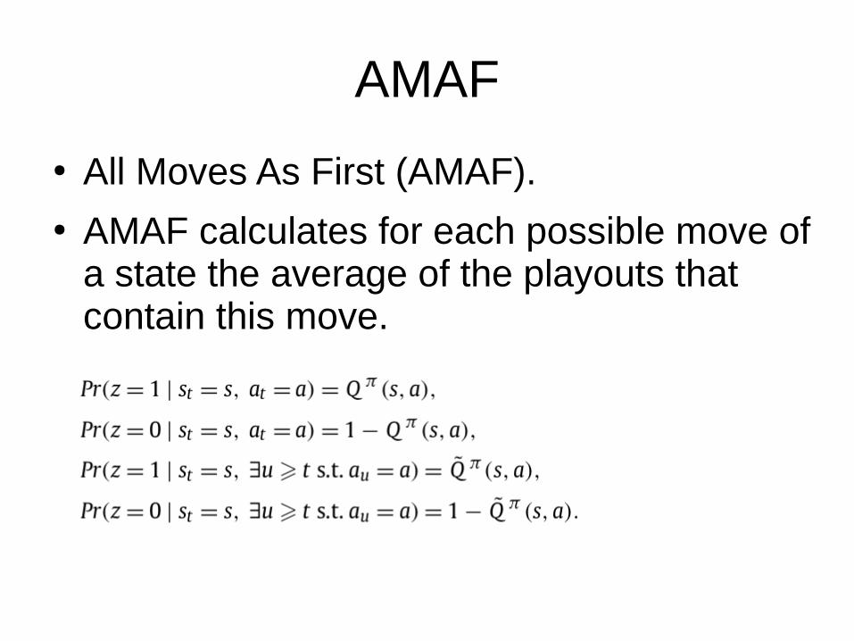
AMAF
● All Moves As First (AMAF).● AMAF calculates for each possible move of
a state the average of the playouts that contain this move.

• Exercise :
• Write a playout function memorizing the played moves.
• Add an integer code for moves in the Move class.
• Add AMAF statistics to the Transposition Table entries.
• Update the AMAF statistics of the Transposition Table.
AMAF

RAVE

RAVE

RAVE

RAVE
RAVE

RAVE

RAVE

• Exercise :
• Compute the AMAF statistics for each node.
• Modify the UCT code to implement RAVE.
RAVE

• State of the art in General Game Playing (GGP)
• Best AI of the Ludii system (https://ludii.games/)
• Simple modification of RAVE
• Uses statistics both for Black and White at all nodes
• “In principle it is also possible to incorporate the AMAF values, from ancestor subtrees. However, in our experiments, combining ancestor AMAF values did not appear to confer any advantage.”
GRAVE

• Use the AMAF statistics of the last ancestor with more than n playouts instead of the AMAF statistics of the current node.
• More accurate when few playouts.
• Published at IJCAI 2015.
• GRAVE is a generalization of RAVE since GRAVE with n=0 is RAVE.
GRAVE


• Exercise :
• Modify the RAVE code to implement GRAVE.
GRAVE

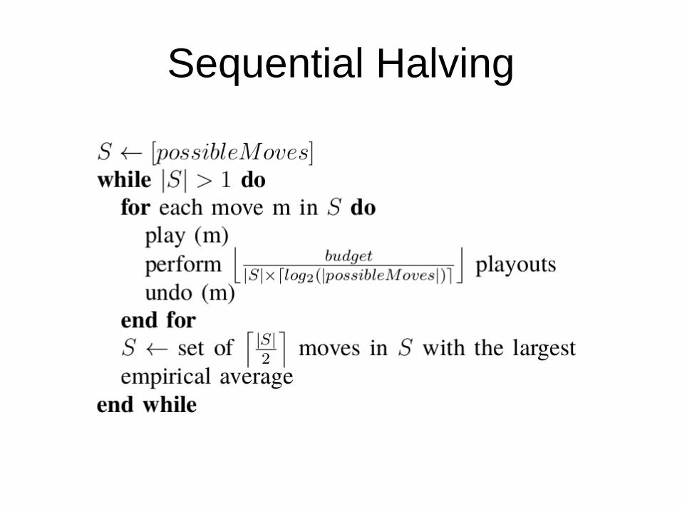
Sequential Halving
● Sequential Halving [Karnin & al. 2013] is a bandit algorithm that minimizes the simple regret.
● It has a fixed budget of arm pulls.● It gives the same number of playouts to all the
arms.● It selects the best half.● Repeat until only one move is left
Sequential Halving

SHOT
● SHOT is the acronym for Sequential Halving Applied to Trees [Cazenave 2015].
● When the search comes back to a node it considers the spent budget and the new budget as a whole.
● It distributes the overall budget with Sequential Halving.

SHOT

SHOT

SHOT
● SHOT gives good results for Nogo.● Combining SHOT and UCT :
SHOT near the rootUCT deeper in the tree
● The combination gives good results for Atarigo, Breakthrough, Amazons and partially observable games.

• Exercise:
• Write the code to perform Sequential Halving at the root on top of UCT.
Sequential Halving

• Sequential Halving combined with other statistics such as AMAF statistics.
• Instead of selecting the best half with the mean (mui), use:
mui + c * AMAFi / pi
with pi the number of playouts of move i and c ≥ 128.
• Combining SH with AMAF = SHUSS (Sequential Halving Using Scores) [Fabiano et al. 2021]
SHUSS

SHUSS

SHUSS

• Exercise:
Write the code to perform SHUSS at the root on top of GRAVE.
SHUSS

PUCT
● MCTS used in AlphaGo and AlphaZero.● A neural network gives a policy and a value.● No playouts, evaluation with the value at the leaves.● P(s,a) = probability for move a of being the best.● Bandit for the tree descent:

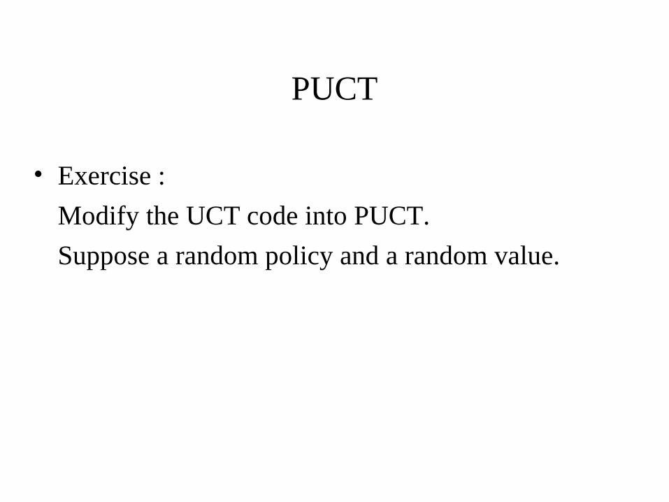
• Exercise :
Modify the UCT code into PUCT.
Suppose a random policy and a random value.
PUCT

Nested Monte Carlo Search
Single Agent Monte Carlo
UCT can be used for single-agent problems. Nested Monte Carlo Search often gives better results. Nested Rollout Policy Adaptation is an
online learning variation that has beaten
world records.

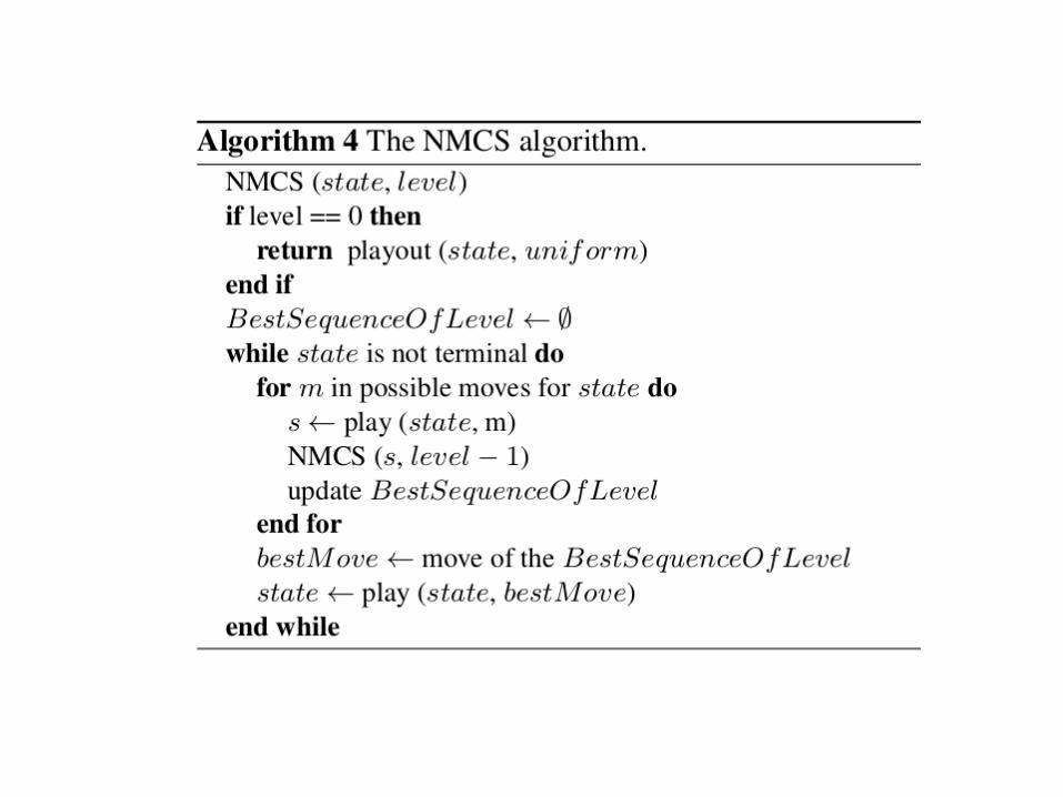
Nested Monte-Carlo Search

• Play random games at level 0
• For each move at level n+1, play the move then play a game at level n
• Choose to play the move with the greatest associated score
• Important : memorize and follow the best sequence found at each level
Nested Monte-Carlo Search

Analysis
• Analysis on two very simple abstract problems.
• Search tree = binary tree.• In each state there are only two possible
moves: going to the left or going to the right.

Analysis• The scoring function of the leftmost path
problem consists in counting the number of moves on the leftmost path of the tree.

Analysis• Sample search : probability 2-n of finding the
best score of a depth n problem. • Depth-first search : one chance out of two of
choosing the wrong move at the root, so the mean complexity > 2n-2.
• A level 1 Nested Monte-Carlo Search will always find the best score, complexity is n(n-1).
• Nested Monte-Carlo Search is appropriate for the leftmost path problem because the scores at the leaves are extremely correlated with the structure of the search tree.

Analysis• The scoring function of the left move
problem consists in counting the number of moves on the left.

Analysis• The probability distribution can be
computed exactly with a recursive formula and dynamic programming.
• A program that plays the left move problems has also been written and results with 100,000 runs are within 1% of the exact probability distribution.

Analysis• Distributions of the scores for a depth 60
problem.

Analysis• Mean score in real time
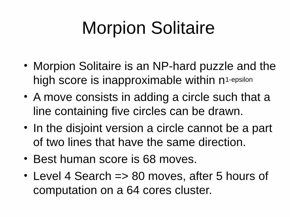
Morpion Solitaire
• Morpion Solitaire is an NP-hard puzzle and the high score is inapproximable within n1-epsilon
• A move consists in adding a circle such that a line containing five circles can be drawn.
• In the disjoint version a circle cannot be a part of two lines that have the same direction.
• Best human score is 68 moves.• Level 4 Search => 80 moves, after 5 hours of
computation on a 64 cores cluster.

Morpion Solitaire• 80 moves :
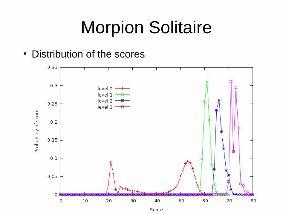
Morpion Solitaire• Distribution of the scores

Morpion Solitaire• Mean scores in real-time

SameGame
• NP-complete puzzle.• It consists in a grid composed of cells of different
colors. Adjacent cells of the same color can be removed together, there is a bonus of 1,000 points for removing all the cells.
• TabuColorRandom strategy: the color that has the most cells is set as the tabu color.
• During the playouts, moves of the tabu color are played only if there are no moves of the others colors or it removes all the cells of the tabu color.

Same Game
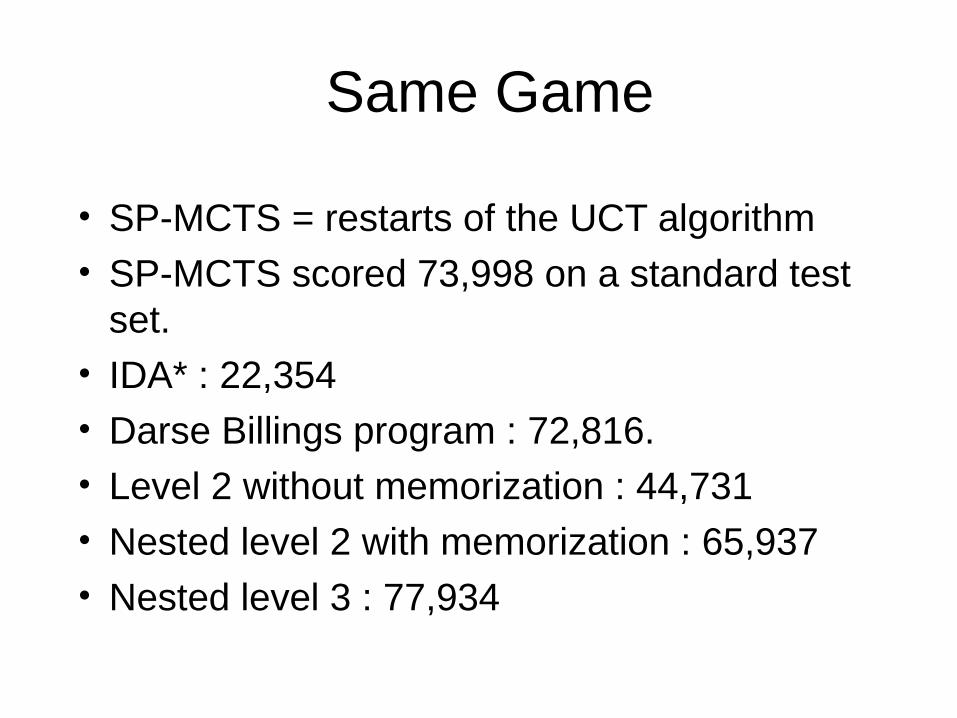
Same Game
• SP-MCTS = restarts of the UCT algorithm • SP-MCTS scored 73,998 on a standard test
set.• IDA* : 22,354• Darse Billings program : 72,816.• Level 2 without memorization : 44,731• Nested level 2 with memorization : 65,937 • Nested level 3 : 77,934

Application to Constraint Satisfaction
• A nested search of level 0 is a playout.• A nested search of level 1 uses a playout
to choose a value.• A nested search of level 2 uses nested
search of level 1 to choose a value.• etc.• The score is always the number of free
variables.

Sudoku
• Sudoku is a popular NP-complete puzzle.• 16x16 grids with 66% of empty cells.• Easy-Hard-Easy distribution of problems.• Forward Checking (FC) is stopped when
the search time for a problem exceeds 20,000 s.

Sudoku
• FC : > 446,771.09 s.• Iterative Sampling : 61.83 s.• Nested level 1 : 1.34 s.• Nested level 2 : 1.64 s.

Kakuro
24 25 20 26 24
18 . . . . .
26 . . . . .
28 . . . . .
26 . . . . .
21 . . . . .
A 5x5 grid
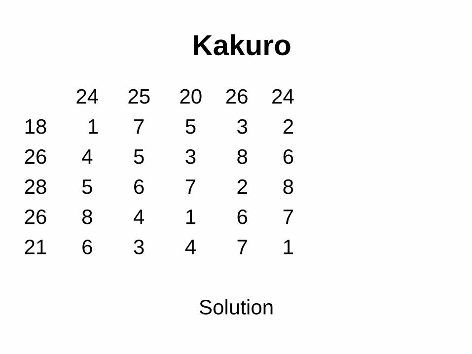
Kakuro
24 25 20 26 24
18 1 7 5 3 2
26 4 5 3 8 6
28 5 6 7 2 8
26 8 4 1 6 7
21 6 3 4 7 1
Solution

Kakuro
Algorithme Solved problems Time
Forward Checking 8/100 92,131.18 s.
Iterative Sampling 10/100 94,605.16 s.
Monte-Carlo level 1 100/100 78.30 s.
Monte-Carlo level 2 100/100 17.85 s.
8x8 Grids, 9 values, stop at 1,000 s.
Bus Regulation
• Goal : minimize passengers waiting times by making buses wait at a stop.
• Evaluation of an algorithm : sum of the waiting times for all passengers.
Regulation Algorithms• Rule-based regulation: The waiting time
depends on the number of stop with the next bus
• Monte-Carlo regulation : Choose the waiting time that has the best mean of random playouts
• Nested Monte-Carlo regulation : Use multiple levels of playouts

Rule-based regulation
• : number of stop before the next bus.
• w : waiting time if the next bus is at more than .
• No regulation : 171 • Wait during 4 if more
than 7 stops : 164

Monte-Carlo Regulation
• 165 for N = 100• 154 for N = 1000• 147 for N = 10000
better than rule-based regulation (164).

Parallel Nested Monte-Carlo Search
• Play the highest level sequentially• Play the lowest levels in parallel• Speedup = 56 for 64 cores at Morpion
Solitaire• A more simple parallelization : play
completely different searches in parallel (i.e. use a different seed for each search).
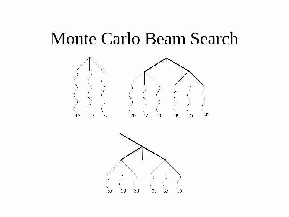
Monte Carlo Beam Search

Single-Agent General Game Playing
• Nested Monte-Carlo search gives better results than UCT on average.
• For some problems UCT is better.
• Ary searches with both UCT and Nested Monte-Carlo search and plays the move that has the best score.

Snake in the box
• A path such that for every node only two neighbors are in the path.
• Applications: Electrical engineering, coding theory, computer network topologies.
• World records with NMCS [Kinny 2012].

Multi-agent pathfinding
• Find routes for the agents avoiding collisions.
• Monte Carlo Fork Search enables to branch in the playouts.
• It solves difficult problems faster than other algorithms [Bouzy 2013].

The Pancake Problem
• Nested Monte Carlo Search has beaten world records using specialized playout policies [Bouzy 2015].
Software Engineering
• Search based software testing [Feldt and Poulding 2015].
• Heuristic Model Checking [Poulding and Feldt 2015].
• Generating structured test data with specific properties [Poulding and Feldt 2014].

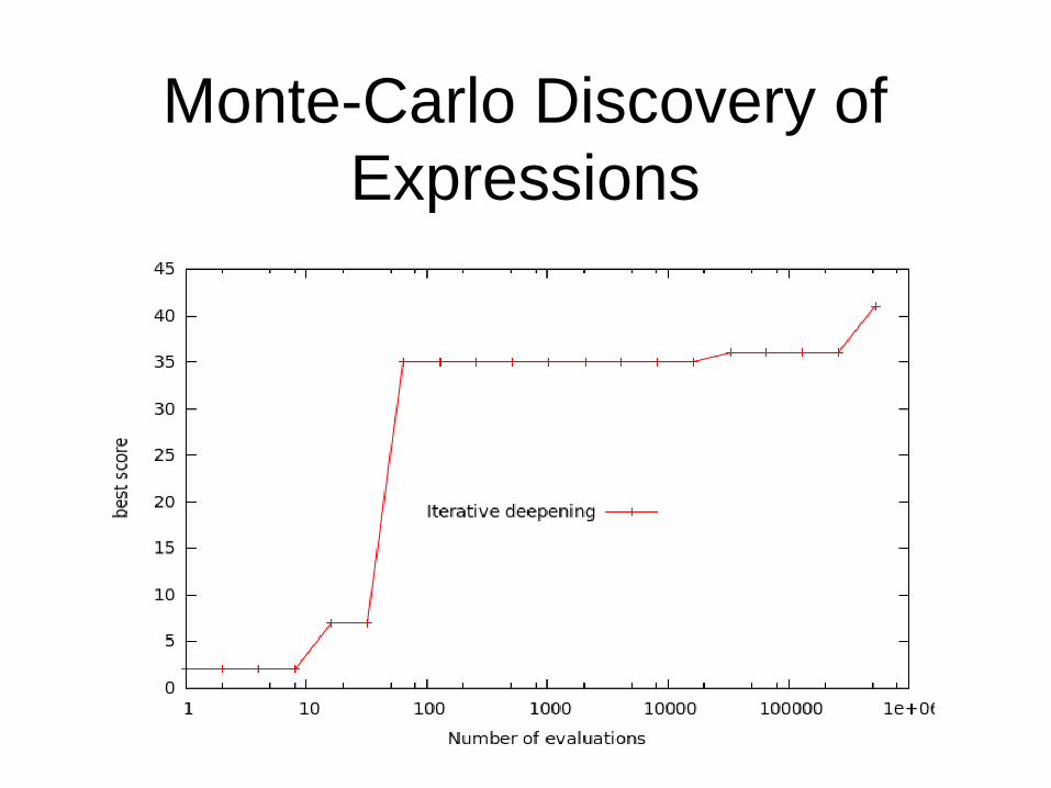
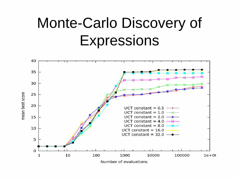
Monte-Carlo Discovery of Expressions
• Possible moves are pushing atoms.
• Evaluation of a complete expression.
• Better than Genetic Programming for some problems [Cazenave 2010, 2013].

Monte-Carlo Discovery of Expressions
Prime Generating Polynomials:
The score of an expression is the number of different primes it generates in a row for integer values of x starting at zero and increasing by one at each step.
Nested Monte-Carlo search is better than UCT and Iterative Deepening search.

Monte-Carlo Discovery of Expressions

Monte-Carlo Discovery of Expressions

Monte-Carlo Discovery of Expressions

Monte-Carlo Discovery of Expressions
N prisoners are assigned with either a 0 or a 1. A prisoner can see the number assigned to the other prisoners but cannot see his own number. Each prisoner is asked independently to guess if he is 0 or 1 or to pass. The prisoners can formulate a strategy before beginning the game. All the prisoners are free if at least one guesses correctly and none guess incorrectly. A possible strategy is for example that one of the prisoners says 1 and the others pass, this strategy has fifty percent chances of winning.

Monte-Carlo Discovery of Expressions
Monte-Carlo Discovery of Expressions
Monte-Carlo Discovery of Expressions
Application to financial data
● Data used to perform our empirical analysis are daily prices of European S&P500 index call options.
● The sample period is from January 02, 2003 to August 29, 2003.
● S&P500 index options are among the most actively traded financial derivatives in the world.

Atom Set
+ Addition C/K Call Price/Strike Price
- Subtraction S/K Index Price/Strike Price
* Multiplication tau Time to Maturity
% Protected Division
ln Protected Natural Log
Exp Exponential function
Sqrt Protected Square Root
cos Cosinus
sin Sinus
Ncfd Normal cumulative distribution

Fitness function
● Each formula found by NMCS or GP is evaluated to test whether it can accurately forecast the implied volatility for all entries in the training set.
● Fitness = Mean Squared Error (MSE) between the estimated volatility and the target volatility.

Mean Square Error

Poor Fitted Observations

RNA Inverse Folding
• Molecule Design as a Search Problem
• Find the sequence of nucleotides that gives a predefined structure.
• A biochimist applied Nested Monte Carlo Search to this problem [Portela 2018].
• Better than the state of the art.
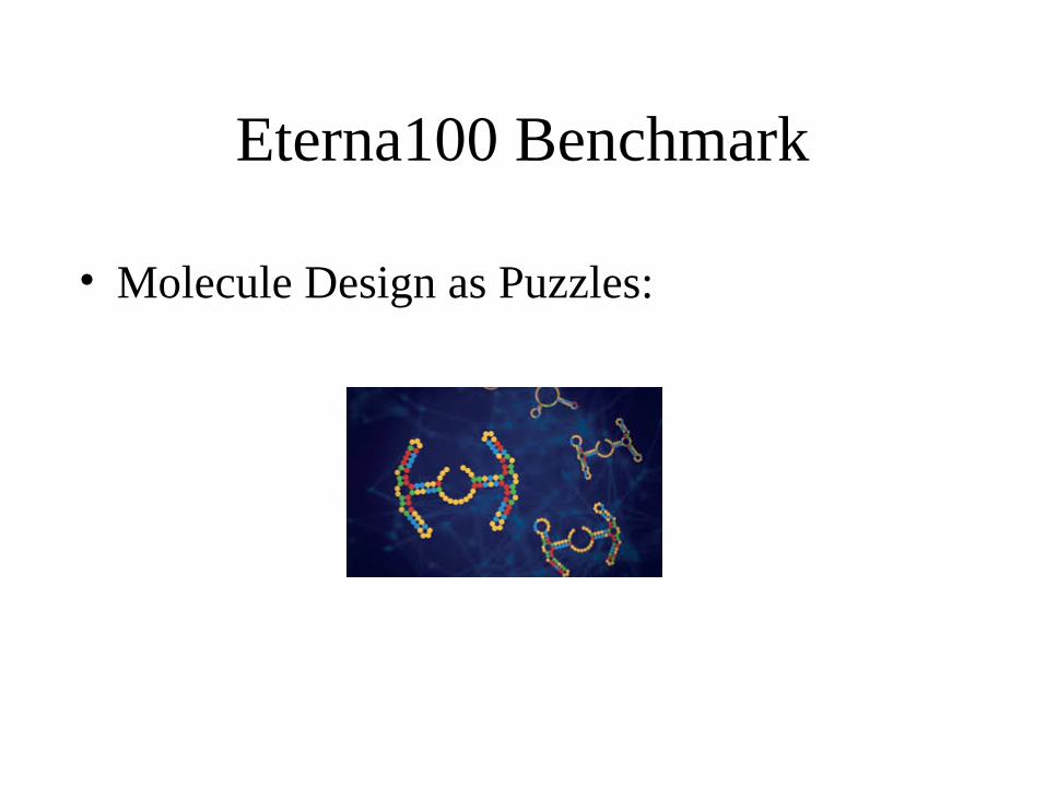
Eterna100 Benchmark
• Molecule Design as Puzzles:

• Write a Nested Monte Carlo Search for the left move problem.
• Functions to write :
legalMoves (state)
play (state, move)
terminal (state)
score (state)
playout (state)
• Then write a Nested Monte Carlo Search using these functions.
Exercise
Exercise :
• Possible atoms : 1, 2, 3, +, -
• Goal : find expressions containing less than 11 atoms that have great evaluations.
• Generate random expressions (i.e. list of atoms).
• Evaluate an expression given as a list of atoms.
• Use NMCS to generate expressions
Expression Discovery

Expression Discovery
+
+
+2
1 3
1
+ + 2 + 1 3 1

• The quality of information propagated during the search can be increased via a discounting heuristic, leading to a better move selection for the overall algorithm.
• Improving the cost-effectiveness of the algorithm without changing the resulting policy by using safe pruning criteria.
• Long-term convergence to an optimal strategy can be guaranteed by wrapping NMCS inside a UCT-like algorithm.
Nested Monte-Carlo Search for Two-player Games

• The discounting heuristic turns a win/loss game into a game with a wide range of outcomes by having the max player preferring short wins to long wins, and long losses to short losses.
• A playout returns v(st) / (t + 1) with v(st) in {-1,1}
Nested Monte-Carlo Search for Two-player Games


Nested Monte-Carlo Search for Two-player Games

Nested Monte-Carlo Search for Two-player Games


• Modify Breakthrough to play Misere Breakthrough.
• Modify playouts for discounted rewards.
• Nested playouts.
• UCT with nested discounted playouts.
• Compare to standard UCT.
Exercise

Nested Rollout Policy Adaptation

Nested Rollout Policy Adaptation
● NRPA [Rosin 2011] is NMCS with policy learning.● It uses Gibbs Sampling as a playout policy.● It adapts the weights of the moves according to
the best sequence of moves found so far.● During adaptation each weight of a move of the
best sequence is incremented and the other moves in the same state are decreased proportionally to the exponential of their weights.

Nested Rollout Policy Adaptation
● Each move is associated to a weight wi
● During a playout each move is played with a probability:
exp (wi) / Sk exp (wk)

Nested Rollout Policy Adaptation
● For each move of the best sequence:
wi = wi + 1
● For each possible move of each state of the best sequence:
wi = wi – exp (wi) / Sk exp (wk)

Morpion Solitaire
World record [Rosin 2011]
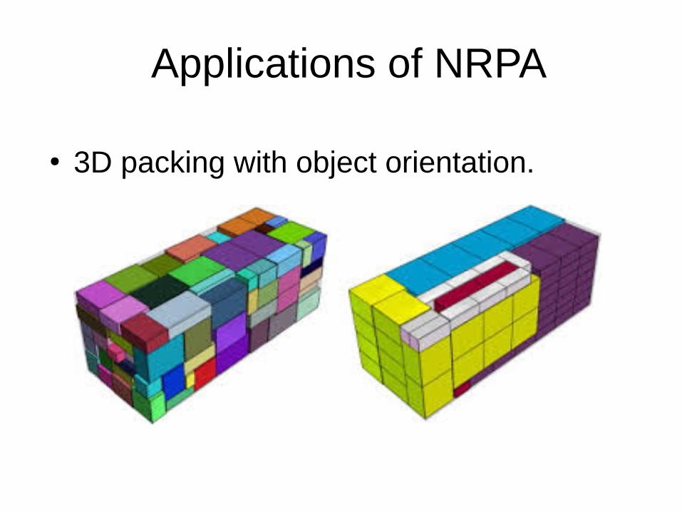
Applications of NRPA
● 3D packing with object orientation.

Applications of NRPA
● Improvement of some alignments for Multiple Sequence Alignment [Edelkamp & al 2015].
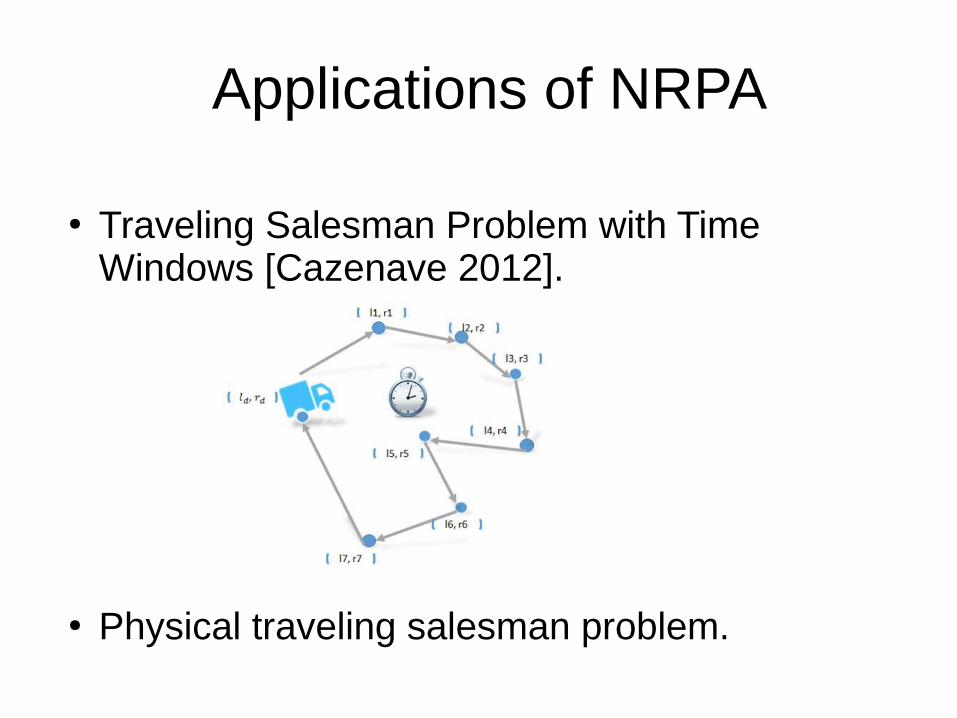
Applications of NRPA
● Traveling Salesman Problem with Time Windows [Cazenave 2012].
● Physical traveling salesman problem.

Applications of NRPA
● State of the art results for Logistics [Edelkamp & al. 2016].
EDF Agents
● EDF fleet of vehicles is one of the largest.● They plan interventions every day.● Monte Carlo Search is 5% better than the
specialized algorithms they use.● Millions of kilometers saved each year.● Hundreds of tons of CO2 each year.
● Morpion Solitaire [Rosin 2011]● CrossWords [Rosin 2011]● Travelling Salesman Problem with Time Windows [Cazenave et al.
2012]● 3D Packing with Object Orientation [Edelkamp et al. 2014]● Multiple Sequence Alignment [Edelkamp et al. 2015]● SameGame [Cazenave et al. 2016]● Vehicle Routing Problems [Edelkamp et al. 2016, Cazenave et al. 2020]● Graph Coloring [Cazenave et al. 2020]● RNA Inverse Folding [Cazenave & Fournier 2020]● …
Nested Rollout Policy Adaptation
Selective Policies
● Prune bad moves during playouts.● Modify the legal moves function.● Use rules to find bad moves.● Different domain specific rules for :
– Bus regulation, – SameGame, – Weak Schur numbers.

Bus Regulation
● At each stop a regulator can decide to make a bus wait before continuing his route.
● Waiting at a stop can reduce the overall passengers waiting time.
● The score of a simulation is the sum of all the passengers waiting time.
● Optimizing a problem is finding a set of bus stopping times that minimizes the score of the simulation.

Bus Regulation
● Standard policy: between 1 and 5 minutes ● Selective policy : waiting time of 1 if there are
fewer than δ stops before the next bus.● Code for a move:
– the bus stop, – the time of arrival to the bus stop,– the number of minutes to wait before leaving the
stop.

Bus Regulation Time No δ δ =3
0.01 2,620 2,147
0.02 2,441 2,049
0.04 2,329 2,000
0.08 2,242 1,959
0.16 2,157 1,925
0.32 2,107 1,903
0.64 2,046 1,868
1.28 1,974 1,811
2.56 1,892 1,754
5.12 1,802 1,703
10.24 1,737 1,660
20.48 1,698 1,640
40.96 1,682 1,629
81.92 1,660 1,617
163.84 1,632 1,610

SameGame
SameGame
● Code of a move = Zobrist hashing.● Tabu color strategy = avoid moves of the
dominant color until there is only one block of the dominant color.
● Selective policy = allow moves of size two of the tabu color when the number of moves already played is greater than t.
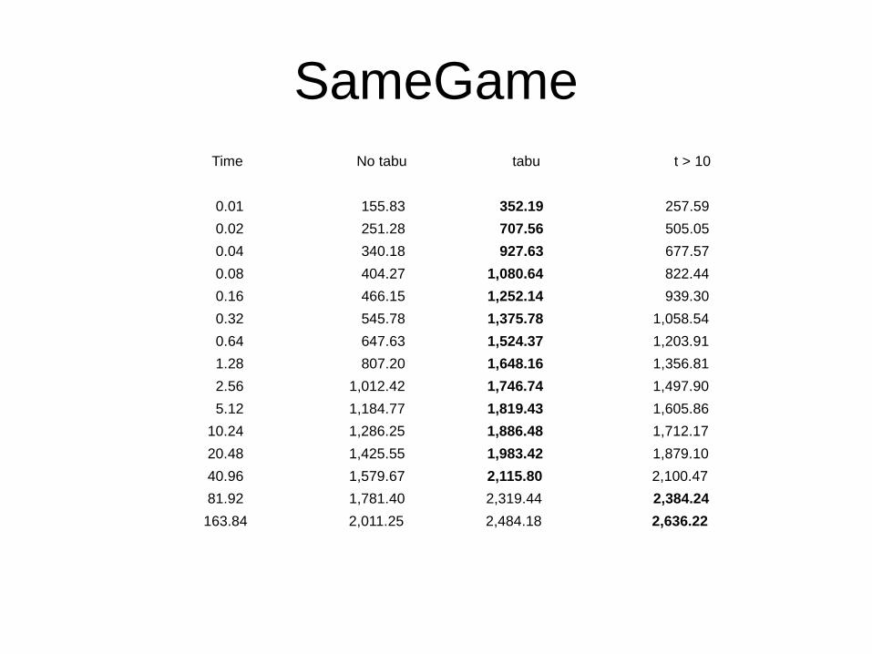
SameGame Time No tabu tabu t > 10
0.01 155.83 352.19 257.59
0.02 251.28 707.56 505.05
0.04 340.18 927.63 677.57
0.08 404.27 1,080.64 822.44
0.16 466.15 1,252.14 939.30
0.32 545.78 1,375.78 1,058.54
0.64 647.63 1,524.37 1,203.91
1.28 807.20 1,648.16 1,356.81
2.56 1,012.42 1,746.74 1,497.90
5.12 1,184.77 1,819.43 1,605.86
10.24 1,286.25 1,886.48 1,712.17
20.48 1,425.55 1,983.42 1,879.10
40.96 1,579.67 2,115.80 2,100.47
81.92 1,781.40 2,319.44 2,384.24
163.84 2,011.25 2,484.18 2,636.22

SameGame
Standard test set of 20 boards:
NMCS SP-MCTS NRPA web
77,934 78,012 80,030 87,858

Same Game
• Hybrid Parallelization [Negrevergne 2017].
• Root Parallelization for each computer. Leaf Parallelization of the playouts using threads.
• New record of 83 050.
• Parallelization for Morpion Solitaire [Nagorko 2019].

Weak Schur Numbers
● Find a partition of consecutive numbers that contains as many consecutive numbers as possible
● A partition must not contain a number that is the sum of two previous numbers in the same partition.
● Partition of size 3 :
1 2 4 8 11 22
3 5 6 7 19 21 23
9 10 12 13 14 15 16 17 18 20

Weak Schur Numbers
● Often a good move to put the next number in the same partition as the previous number.
● If it is legal to put the next number in the same partition as the previous number then it is the only legal move considered.
● Otherwise all legal moves are considered.● The code of a move for the Weak Schur problem
takes as input the partition of the move, the integer to assign and the previous number in the partition.

Weak Schur Numbers Time ws(9) ws-rule(9)
0.01 199 2,847
0.02 246 3,342
0.04 263 3,717
0.08 273 4,125
0.16 286 4,465
0.32 293 4,757
0.64 303 5,044
1.28 314 5,357
2.56 331 5,679
5.12 362 6,065
10.24 384 6,458
20.48 403 6,805
40.96 422 7,117
81.92 444 7,311
163.84 473 7,538

Selective Policies
● We have applied selective policies to three quite different problems.
● For each problem selective policies improve NRPA.
● We used only simple policy improvements.● Better performance could be obtained
refining the proposed policies.


Exercise ● Apply NRPA to the Left Move problem.● Write a function playout (state) that plays a playout
using Gibbs sampling.● The probability of playing a move is proportional to the
exponential of the weight of the move.● weight is a dictionary that contains the weights of the
moves.● Write the Adapt function● Write the NRPA function

Exercise
● Apply NRPA to the Weak Schur problem.● Write a function that plays a playout using Gibbs
sampling.● The probability of playing a move is proportional to
the exponential of the weight of the move.● weight is a dictionary that contains the weights
associated to the moves.● code (move) returns the integer associated to the
move in the weight dictionary.

Exercise
● Write the adapt function that modifies the weights of the moves according to the best sequence of moves.
● Weights of the moves of the best sequence are incremented.
● For each state of the best sequence, weights of all the moves are reduced proportional to their probabilities.

Exercise
● Write the multi level NRPA code that retains a best sequence per level and recursively calls lower levels.
● Level zero is a playout with Gibbs sampling.

Analysis of Nested Rollout Policy Adaptation

Generalized Nested Rollout Policy Adaptation

Generalized Nested Rollout Policy Adaptation

Generalized Nested Rollout Policy Adaptation

Generalized Nested Rollout Policy Adaptation
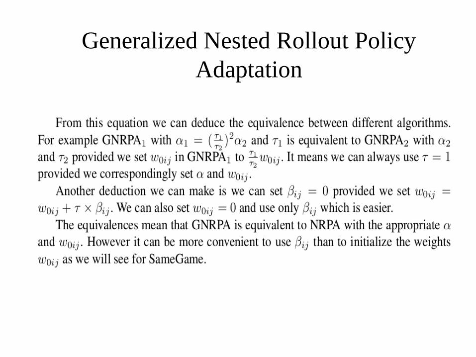
Generalized Nested Rollout Policy Adaptation

SameGame

TSPTW

TSPTW
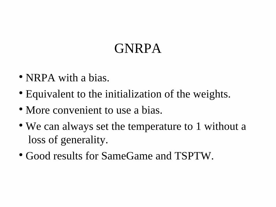
GNRPA
● NRPA with a bias.● Equivalent to the initialization of the weights.● More convenient to use a bias.● We can always set the temperature to 1 without a
loss of generality.● Good results for SameGame and TSPTW.

GNRPA
● Exercise:● Apply GNRPA to the Weak Schur problem.

Eterna 100
● Find a sequence that has a given folding

Eterna 100
● Human experts have managed to solve the 100 problems of the benchmark● No program has so far achieved such a score.● The best score so far is 95/100 by NEMO:
NEsted MOnte Carlo RNA Puzzle Solver

NEMO
● NEMO uses two sets of heuristics● General ones that give probabilities to pairs of bases.● More specific ones that are tailored to puzzle solving.

GNRPA
Other Improvements
● Stabilized GNRPA● Beam GNRPA● Zobrist Hashing● Restarts● Parallelization

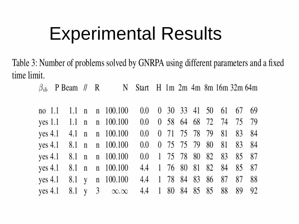
Experimental Results

Experimental Results
● Leaf Parallelization
Experimental Results

Experimental Results
● Root Parallelization

Conclusion
● 95/100 problems solved, same as NEMO.● Less domain knowledge.● Various improvements of NRPA.

Playout Policy Adaptation

Offline learning of a playout policy
● Offline learning of playout policies has given good results in Go [Coulom 2007, Huang 2010] and Hex [Huang 2013], learning fixed pattern weights so as to bias the playouts.
● Patterns are also used to do progressive widening in the UCT tree.

Online learning of a playout policy
● The RAVE algorithm [Gelly 2011] performs online learning of moves values in order to bias the choice of moves in the UCT tree.
● RAVE has been very successful in Go and Hex. ● A development of RAVE is to use the RAVE values to
choose moves in the playouts using Pool RAVE [Rimmel 2010].
● Pool RAVE improves slightly on random playouts in Havannah and reaches 62.7% against random playouts in Go.
Online learning of a playout policy
● Move-Average Sampling Technique (MAST) is a technique used in the GGP program Cadia Player so as to bias the playouts with statistics on moves [Finnsson 2010].
● It consists of choosing a move in the playout proportionally to the exponential of its mean.
● MAST keeps the average result of each action over all simulations.

Online learning of a playout policy
● Later improvements of Cadia Player are N-Grams and the last good reply policy [Tak 2012].
● They have been applied to GGP so as to improve playouts by learning move sequences.
● A recent development in GGP is to have multiple playout strategies and to choose the one which is the most adapted to the problem at hand [Swiechowski 2014].

Online learning of a playout policy
● Playout Policy Adaptation (PPA) also uses Gibbs sampling.
● The evaluation of an action for PPA is not its mean over all simulations such as in MAST.
● Instead the value of an action is learned comparing it to the other available actions for the state where it has been played.
Playout Policy learning
● Start with a uniform policy.
● Use the policy for the playouts.
● Adapt the policy for the winner of each playout.
Playout Policy learning
● Each move is associated to a weight wi.
● During a playout each move is played with a probability :
exp (wi) / Sk exp (wk)

Playout Policy learning
● Online learning :● For each move of the winner :
wi = wi + 1
● For each possible move of each state of the winner :
wi = wi – exp (wi) / Sk exp (wk)

Breakthrough
● The first player to reach the opposite line has won

Misère Breakthrough
● The first player to reach the opposite line has lost

Knightthrough
● The first to put a knight on the opposite side has won.
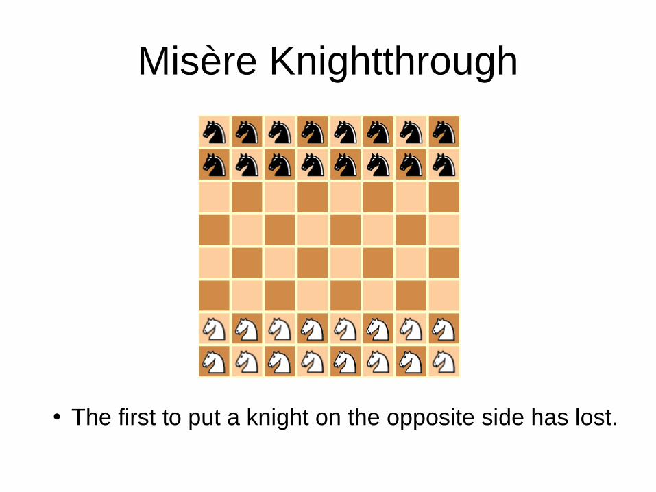
Misère Knightthrough
● The first to put a knight on the opposite side has lost.
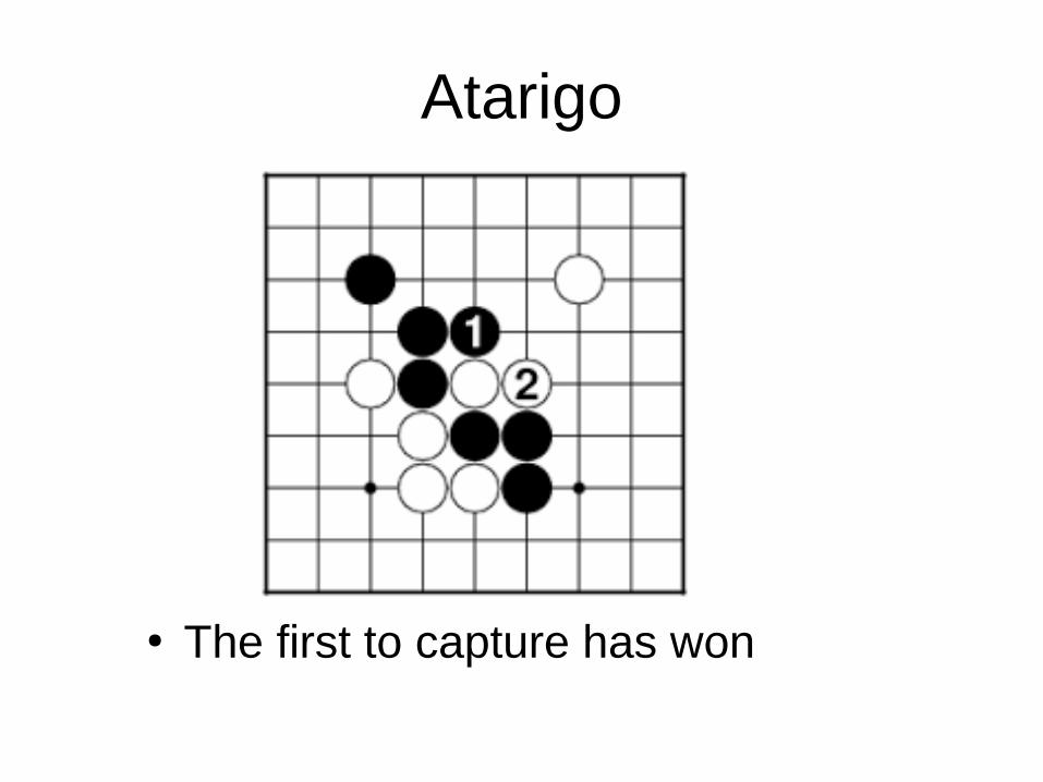
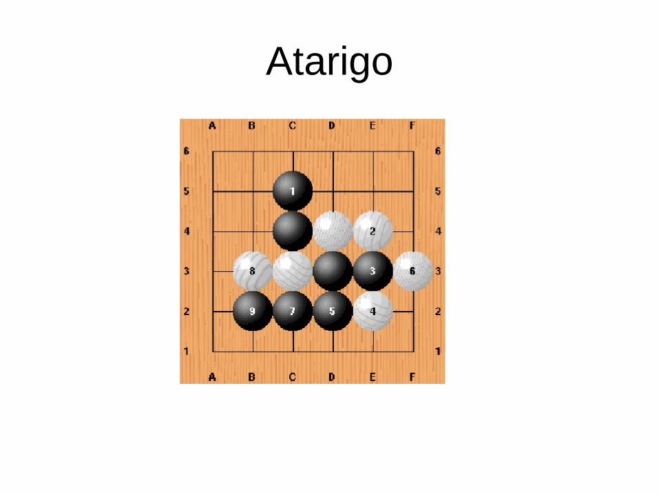
Atarigo
● The first to capture has won
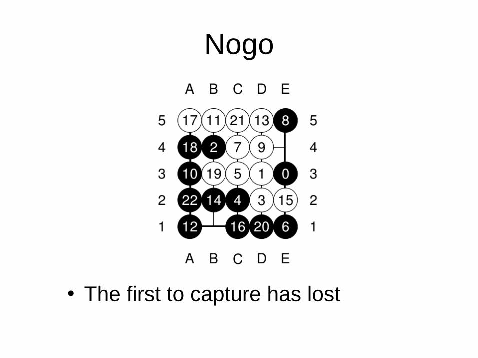
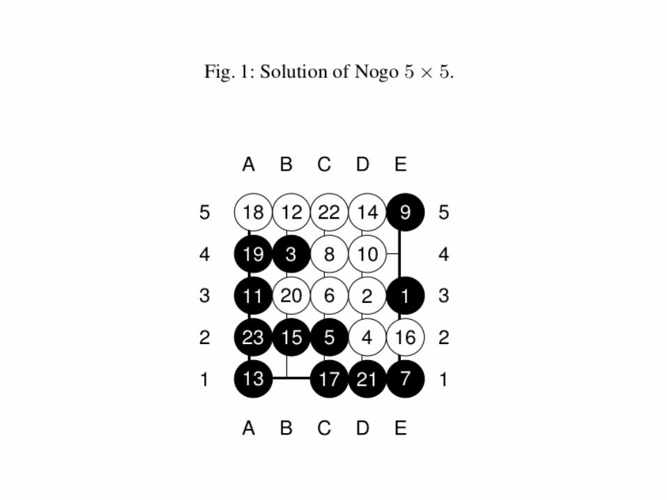
Nogo
● The first to capture has lost

Domineering Misère Domineering
● The last to play has won / lost.
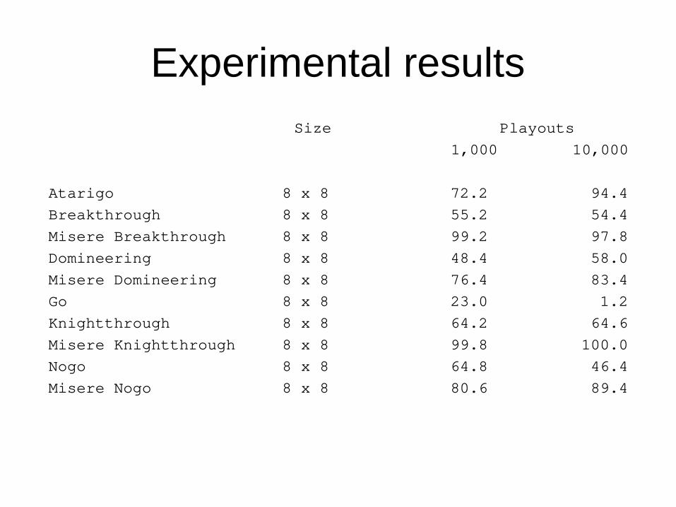
Experimental results Size Playouts 1,000 10,000
Atarigo 8 x 8 72.2 94.4Breakthrough 8 x 8 55.2 54.4 Misere Breakthrough 8 x 8 99.2 97.8Domineering 8 x 8 48.4 58.0Misere Domineering 8 x 8 76.4 83.4Go 8 x 8 23.0 1.2Knightthrough 8 x 8 64.2 64.6Misere Knightthrough 8 x 8 99.8 100.0Nogo 8 x 8 64.8 46.4Misere Nogo 8 x 8 80.6 89.4

Playout Policy learning with Move Features
● Associate features to the move.
● A move and its features are associated to a code.
● The algorithm learns the weights of codes instead of simply the weights of moves.

Playout Policy learning with Move Features
● Atarigo : four adjacent intersections● Breakthrough : capture in the move code● Misère Breakthrough : same as Breakthrough● Domineering : cells next to the domino played● Misère Domineering : same as Domineering● Knightthrough : capture in the move code● Misère Knighthrough : same as Knighthrough● Nogo : same as Atarigo

Experimental results
● Each result is the outcome of a 500 games match, 250 with White and 250 with Black.
● UCT with an adaptive policy (PPAF) is played against UCT with a random policy.
● Tests are done for 10,000 playouts.● For each game we test size 8x8.● We tested 8 different games.

Experimental results Size Winning %
Atarigo 8 x 8 94.4 %
Breakthrough 8 x 8 81.4 %
Misere Breakthrough 8 x 8 100.0 %
Domineering 8 x 8 80.4 %
Misere Domineering 8 x 8 93.0 %
Knightthrough 8 x 8 84.0 %
Misere Knightthrough 8 x 8 100.0 %
Nogo 8 x 8 95.4 %

PPAF and Memorization
● Start a game with an uniform policy.
● Adapt at each move of the game.
● Start at each move with the policy of the previous move.

PPAF and Memorization
● A nice property of PPAF is that the move played after the algorithm has been run is the most simulated move.
● The memorized policy is related to the state after the move played by the algorithm since it is the most simulated move.
● When starting with the memorized policy for the next state, this state has already been partially learned

PPAFM versus PPAF uniform
Game Score
Atarigo 66.0%
Breakthrough 87.4%
Domineering 58.0%
Knightthrough 84.6%
Misere Breakthrough 97.2%
Misere Domineering 56.8%
Misere Knightthrough 99.2%
Nogo 49.4%

PPAFM versus UCT
Game Score
Atarigo 95.4%
Breakthrough 94.2%
Domineering 81 .8%
Knightthrough 96.6%
Misere Breakthrough 100.0%
Misere Domineering 95.8%
Misere Knightthrough 100.0%
Nogo 91.6%

PPA Adapt Algorithm

• Try PPA for Misere Breakthrough.– The playout function
– The adapt function
– Combination with UCT
• Take capture into account (PPAF).
• Memorize the policy (PPAFM).
• Compare to UCT.
Exercise

• Modify GRAVE to incorporate a policy and a bias.
• Use the AMAF statistics of the root node of GRAVE to bias the playouts as in GNRPA.
• Update the Adapt to take the bias into account.
• Write the main function that calls GRAVEPolicyBias and updates the policy.
Exercise
Outline
● Algorithm for solving games● GRAVE and PPAF● Monte Carlo move ordering● Experiments● Conclusion

Solving Games
● Proof-Number Search (PN)● PN2
● Alpha-Beta● Iterative Deepening Alpha-Beta● Retrograde Analysis

UCT
RAVE
● A big improvement for Go, Hex and other games is Rapid Action Value Estimation (RAVE) [Gelly and Silver 2007].
● RAVE combines the mean of the playouts that start with the move and the mean of the playouts that contain the move (AMAF).
RAVE
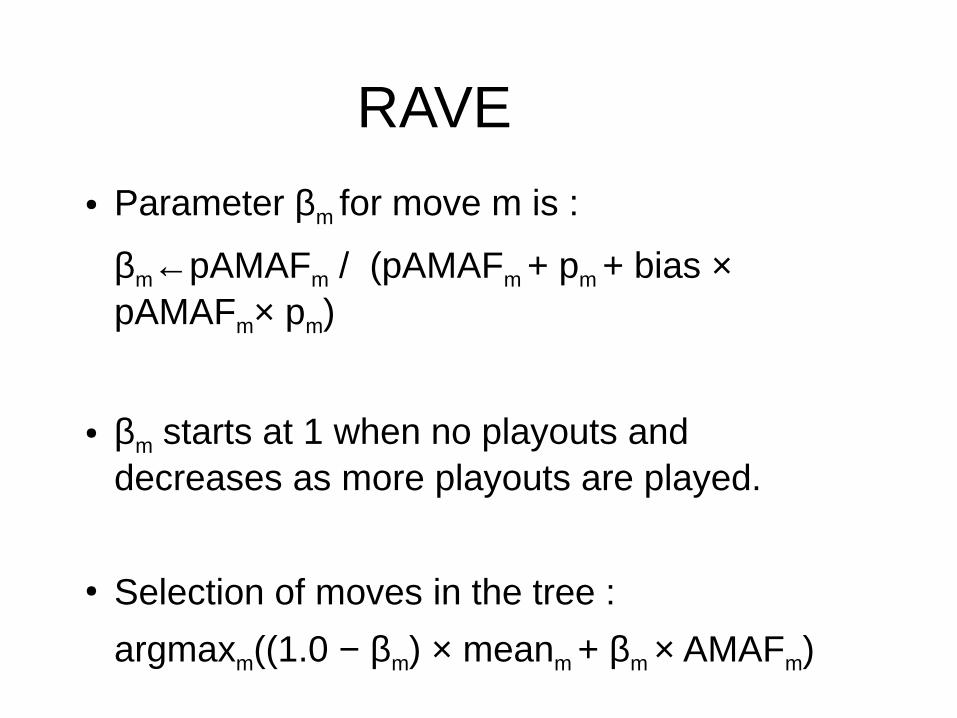
● Parameter βm for move m is :
βm←pAMAFm / (pAMAFm + pm + bias × pAMAFm× pm)
● βm starts at 1 when no playouts and decreases as more playouts are played.
● Selection of moves in the tree :
argmaxm((1.0 − βm) × meanm + βm × AMAFm)
GRAVE● Generalized Rapid Action Value
Estimation (GRAVE) is a simple modification of RAVE.
● It consists in using the first ancestor node with more than n playouts to compute the RAVE values.
● It is a big improvement over RAVE for Go, Atarigo, Knightthrough and Domineering [Cazenave 2015].

Playout Policy learning
● Start with a uniform policy.
● Use the policy for the playouts.
● Adapt the policy for the winner of each playout.

Playout Policy learning
● Each move is associated to a weight wi.
● During a playout each move is played with a probability :
exp (wi) / Sk exp (wk)

Playout Policy learning
● Online learning :● For each move of the winner :
wi = wi + 1
● For each possible move of each state of the winner :
wi = wi – exp (wi) / Sk exp (wk)

Monte Carlo Game Solver
● Use the order of moves of GRAVE when the state is in the GRAVE tree.
● Use the order of moves of Playout Policy Adaptation when the state is outside the GRAVE tree.


Conclusion● For the games we solved, Misere Games are more difficult to solve
than normal games.● In Misere Games the player waits and tries to force the opponent to
play a losing move.● This makes the game longer and reduces the number of winning
sequences and winning moves.● Monte Carlo Move Ordering improves much the speed of αβ with
transposition table compare to depth first αβ and Iterative Deepening αβ with transposition table but without Monte Carlo Move Ordering.
● The experimental results show significant improvements for nine different games.

Zero Learning

Deep Reinforcement Learning
• AlphaGo
• Golois
• AlphaGo Zero
• Alpha Zero
• Mu Zero
• Polygames

David Silver Aja Huang
AlphaGo
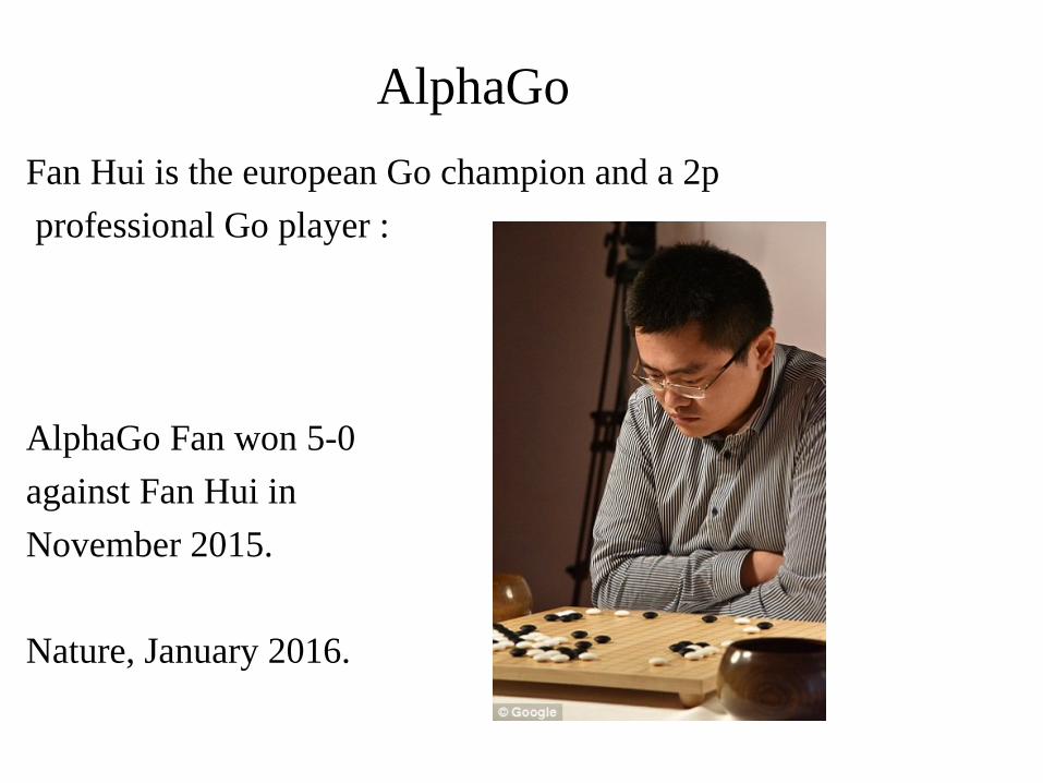
Fan Hui is the european Go champion and a 2p
professional Go player :
AlphaGo Fan won 5-0
against Fan Hui in
November 2015.
Nature, January 2016.

AlphaGo
Lee Sedol is among the strongest and most famous
9p Go player :
AlphaGo Lee won 4-1 against Lee Sedol in march
2016.

AlphaGo
Ke Jie is the world champion of Go according to
Elo ratings :
AlphaGo Master
won 3-0 against
Ke Jie in
may 2017.

AlphaGo
AlphaGo Zero learns to play Go from scratch playing against itself.
After 40 days of self play it surpasses AlphaGo Master.
Nature, 18 october 2017.
AlphaGo
• AlphaGo combines MCTS and Deep Learning.
• There are four phases to the development of AlphaGo :
• Learn strong players moves => policy network.
• Play against itself and improve the policy network => reinforcement learning.
• Learn a value network to evaluate states from millions of games played against itself.
• Combine MCTS, policy and value network.

AlphaGo

AlphaGo

AlphaGo
• The policy network is a 13 layers network.
• It uses either 128 or 256 feature planes.
• It is fully convolutional.
• It learns to predict moves from hundreds of thousands of strong players games.
• Once it has learned, it finds the strong player move 57.0 % of the time.
• It takes 3 ms to run.
AlphaGo
• The value network is also a deep convolutional neural network.
• AlphaGo played a lot of games and kept for each game a state and the corresponding terminal state.
• It learns to evaluate states with the result of the terminal state.
• The value network has learned an evaluation function that gives the probability of winning.

AlphaGo

AlphaGo

AlphaGo
• The policy network is used as a prior to consider good moves at first.
• Playouts are used to evaluate moves
• The value network is combined with the statistics of the moves coming from the playouts.
• PUCT :

AlphaGo

AlphaGo
• AlphaGo has been parallelized using a distributed version.
• 40 search threads, 1,202 CPUs and 176 GPU.

AlphaGo

AlphaGo

AlphaGo

AlphaGo

AlphaGo

Golois

Golois
• I replicated the AlphaGo experiments with the policy and value networks.
• Golois policy network scores 58.54% on the test set (57.0% for AlphaGo).
• Golois plays on the kgs internet Go server.
• It has a strong 4d ranking just with the learned policy network (AlphaGo policy network is 3d).

Data
● Learning set = games played on the KGS Go server by players being 6d or more between 2000 and 2014.
● No handicap games. ● Each position is rotated to eight possible symmetric
positions. ● 160 000 000 positions in the learning set. ● Test set = games played in 2015. ● 100 000 different positions not mirrored.
Training● In order to train the network we build minibatches of size 50
composed of 50 states chosen randomly in the training set.● Each state is randomly mirrored to one of its eight
symmetric states. ● We define an epoch as 5 000 000 training examples.● The accuracy and the error on the test set are computed
every epoch. ● The learning rate is divided by two each time the training
error stalls, i.e. is greater than the previous average training error over the last epoch.

Residual Nets
• Residual Nets :
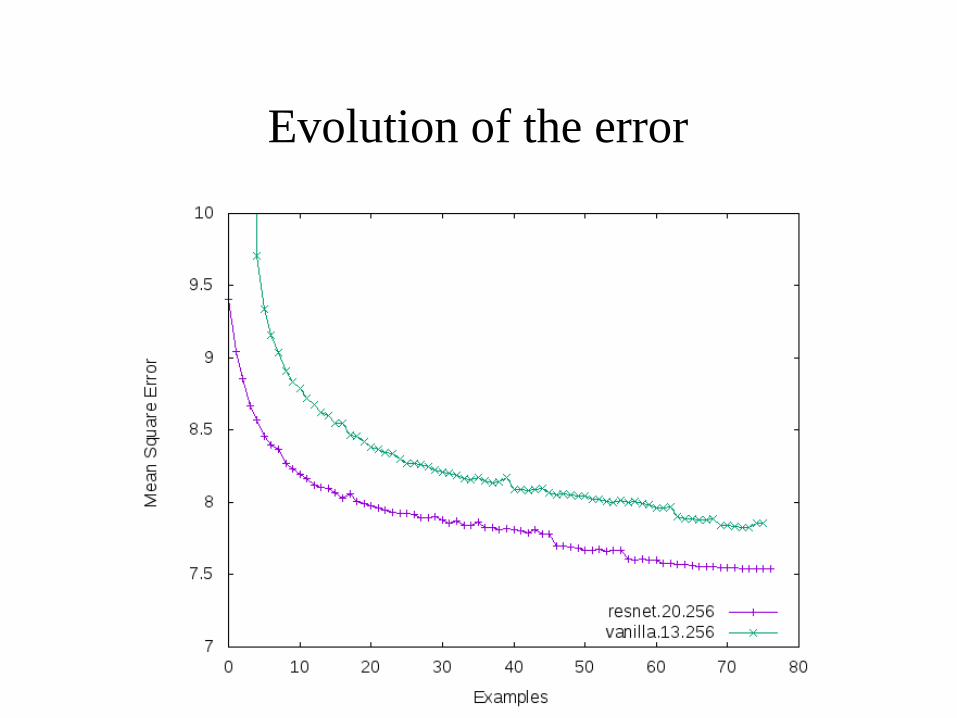
Evolution of the error

Evolution of the accuracy

Golois Policy Network
• Using residual network enables to train deeper network.
• It enables better accuracy than AlphaGo policy network.
• It has a 4 dan level on kgs, playing moves instantly.
• Next: value network and parallel MCTS.

Batch Normalization

Usual Layer
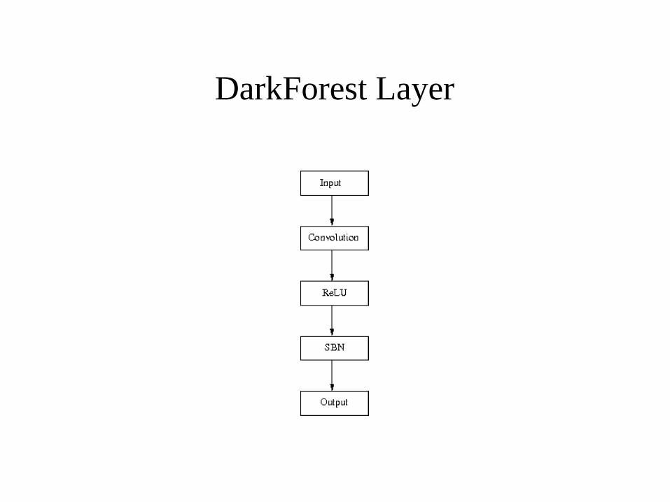
DarkForest Layer

Residual Layer
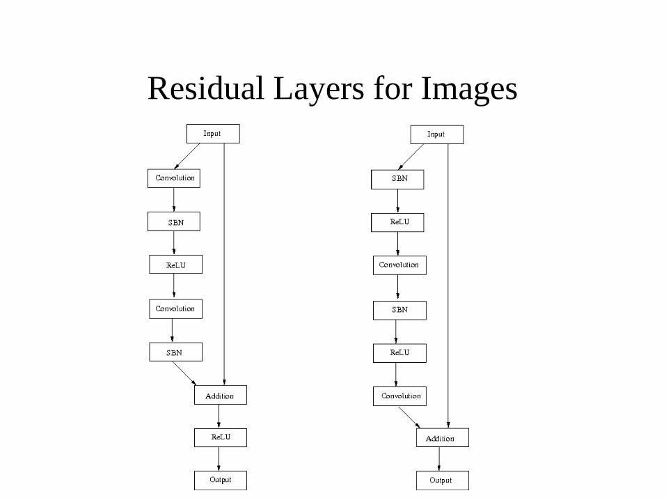
Residual Layers for Images

Golois Layer
Multiple Output Planes
● In DarkForest it improves the level of play to predict the next three moves instead of only the next move.
● We compared the next move prediction and the next three moves prediction with the Golois layer.

Data
● We use the GoGoD dataset.● It is composed of many professional games played
until today.● We used the games from 1900 to 2014 for the
training set and the games from 2015 and 2016 as the test set.
● The first 500 000 positions of the test set to evaluate the error and the accuracy of the networks.

Multiple Output Planes
● Evolution of the accuracy for 1 and 3 output planes

Multiple Output Planes
● Evolution of the errors for one output plane

Multiple Output Planes
● Evolution of the errors for three output planes
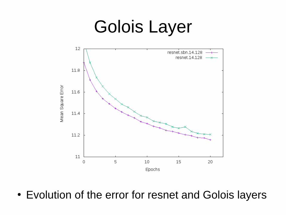
Golois Layer
● Evolution of the error for resnet and Golois layers

Golois Layer
● Evolution of the accuracy for resnet and Golois layers

Golois Layer
● Evolution of the error for different layers

Golois Layer
● Multiple Output Planes improves the generalization of residual networks.
● Spatial Batch Normalization helps train the residual network faster and obtain better accuracy.

Value Network
● The Golois policy network played 1,600,000 games against itself.
● 20 layers residual value network trained on these games.
● Parallel PUCT with policy and value networks.● No playouts.● Using this value network Golois reached 8d.● ELF network => 9d.

AlphaGo Zero

AlphaGo Zero
● AlphaGo Zero starts learning from scratch.
● It uses the raw representation of the board as input, even liberties are not used.
● It has 15 input planes, 7 for the previous Black stones, 7 for the previous White Stones and 1 plane for the color to play.

AlphaGo Zero
● It plays against itself using PUCT and 1,600 tree descents per move.
● It uses a residual neural network with two heads.
● One head is the policy, the other head is the value.

AlphaGo Zero

AlphaGo Zero
● After 4.9 million games against itself a 20 residual blocks neural network reaches the level of AlphaGo Lee (100-0).
● 3 days of self play on the machines of DeepMind.● Comparison : Golois searches 1,600 nodes in 10
seconds on a 4 GPU machine.● It would take Golois 466 years to play 4.9 million such
games.

AlphaGo Zero

AlphaGo Zero

AlphaGo Zero
● They used a longer experiment with a deeper network.● 40 residual blocks.● 40 days of self play on the machines of DeepMind.● In the end it beats Master 89-11.

AlphaGo Zero
AlphaGo Zero

AlphaGo Zero
● AlphaGo Zero uses 40 residual blocks instead of 20 blocks for AlphaGo Master.
● With 20 blocks learning stalls after 3 days.● Master with 40 blocks better than AlphaGo Zero?
Alpha Zero
Alpha Zero
● Arxiv, 5 december 2017.
● Deep reinforcement learning similar to AlphaGo Zero.
● Same algorithm applied to two other games :
Chess and Shogi.
● Learning from scratch without prior knowledge.

Alpha Zero
● Alpha Zero surpasse Stockfish at Chess after 4 hours of self-play.
● Alpha Zero surpasses Elmo at shogi after 2 hours of self play.

Alpha Zero
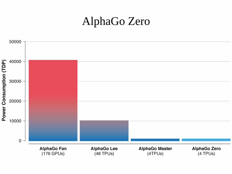
● 5 000 first generation TPU for training.
●4 TPU for playing.

Mu Zero

Mu Zero
● Arxiv, december 2019.
● Similar to Alpha Zero without knowing the rules of the games.
● Atari, Go, Chess and Shogi.
● Learning from scratch without prior knowledge.
Polygames

Polygames
● Alpha Zero approach for many games.
● A common interface to all the games.
● Fully convolutional network, average pooling…
● Pytorch and C++.
● Open source !
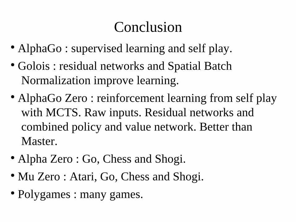
Conclusion● AlphaGo : supervised learning and self play.● Golois : residual networks and Spatial Batch
Normalization improve learning.● AlphaGo Zero : reinforcement learning from self play
with MCTS. Raw inputs. Residual networks and combined policy and value network. Better than Master.
● Alpha Zero : Go, Chess and Shogi.● Mu Zero : Atari, Go, Chess and Shogi. ● Polygames : many games.

Alpha Zero

Alpha Zero
● Define a network that takes as input the Breakthrough board and gives as output the policy and the value for the board.
● Bias the MCTS with policy and value using PUCT.● Make the network play games and record the results
of the Monte Carlo and the result of the games.● Train the network on the results of the games.● Iterate.

Alpha Zero● The network takes 41 inputs with values 0 or 1, 20 inputs
for black pawns, 20 inputs for white pawns and one input for the color to play.
● Option: also use previous boards as inputs.● The network has 60 outputs for the policy head (3 possible
moves for each cell), and 1 output for the value head.● The architecture of the network can be completely
connected as a starting point.● Option : convolutional network, residual network.

Alpha Zero
1) Define the network
2) Implement the PUCT algorithm using the network. Use the same network for black and white, rotate the board for white so that moves are always forward.
3) Make the algorithm play against itself.
4) Record the Monte Carlo distributions and the result of self played games.
5) Train the network on the recorded data.

• Transformer une position de breakthrough 5x5 en trois matrices 5x5 de 0 et de 1 (Noir/Blanc/Vide).
• Faire deux réseaux convolutifs (blanc et noir) avec 76 sorties (75 coups possibles + évaluation) et ces trois matrices en entrée.
• Utiliser les réseaux dans PUCT pour politique et évaluation.
• Faire jouer à PUCT >100 parties contre lui même.
• Mémoriser pour chaque position un vecteur de 76 réels entre 0 et 1 (une fréquence pour chaque code de coup entre 0 et 75, code = 3 *(5 * x + y) + 0, 1 ou 2) et un réel (1.0 si blanc a gagné, 0.0 sinon).
• Entraîner les deux réseaux convolutifs pour retrouver les fréquences et le résultat de la partie en sortie pour chaque position en entrée.
• Itérer.
Projet Python
Monte Carlo Search with Imperfect Information
Information Set MCTS
● Flat Monte Carlo Search gives good results for Phantom Go.
● Information Set MCTS.● Card games.

Counter Factual Regret Minimization
● Poker : Libratus (CMU), DeepStack (UofA).● Approximation of the Nash Equilibrium.● There are about 320 trillion “information sets” in heads-
up limit hold’em.● What the algorithm does is look at all strategies that do
not include a move, and count how much we “regret” having excluded the move from our mix.
● Combination with neural networks.● Better than top professional players.

αμ
● Bridge● Generate a set of possible worlds.● Solve each world exactly● Search multiple moves ahead● Strategy Fusion => joint search● Non Locality => Pareto fronts
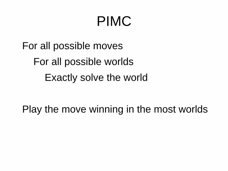
PIMC
For all possible moves
For all possible worlds
Exactly solve the world
Play the move winning in the most worlds

Strategy Fusion
● Problem = PIMC can play different moves in different worlds.
● Whereas the player cannot distinguish between the different worlds.

Non Locality
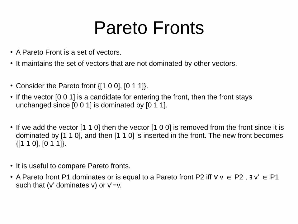
Pareto Fronts● A Pareto Front is a set of vectors.● It maintains the set of vectors that are not dominated by other vectors.
● Consider the Pareto front {[1 0 0], [0 1 1]}. ● If the vector [0 0 1] is a candidate for entering the front, then the front stays
unchanged since [0 0 1] is dominated by [0 1 1].
● If we add the vector [1 1 0] then the vector [1 0 0] is removed from the front since it is dominated by [1 1 0], and then [1 1 0] is inserted in the front. The new front becomes {[1 1 0], [0 1 1]}.
● It is useful to compare Pareto fronts. ● A Pareto front P1 dominates or is equal to a Pareto front P2 iff v P2 , v’ P1 ∀ ∈ ∃ ∈
such that (v’ dominates v) or v’=v.

AlphaMu
● At Max nodes each possible move returns a Pareto front.
● The overall Pareto front is the union of all the Pareto fronts of the moves.
● The idea is to keep all the possible options for Max, i.e. Max has the choice between all the vectors of the overall Pareto front.
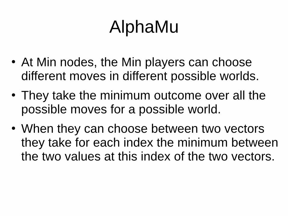
AlphaMu
● At Min nodes, the Min players can choose different moves in different possible worlds.
● They take the minimum outcome over all the possible moves for a possible world.
● When they can choose between two vectors they take for each index the minimum between the two values at this index of the two vectors.
AlphaMu● When Min moves lead to Pareto fronts, the Max player can
choose any member of the Pareto front. ● For two possible moves of Min, the Max player can also choose
any combination of a vector in the Pareto front of the first move and of a vector in the Pareto front of the second move.
● Compute all the combinations of the vectors in the Pareto fronts of all the Min moves.
● For each combination the minimum outcome is kept so as to produce a unique vector.
● Then this vector is inserted in the Pareto front of the Min node.
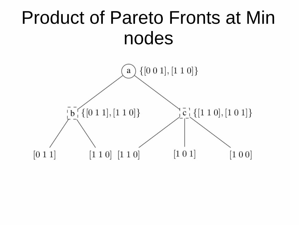
Product of Pareto Fronts at Min nodes

The Early Cut

The Root Cut
● If a move at the root of αμ for M Max moves gives the same probability of winning than the best move of the previous iteration of iterative deepening for M-1 Max moves, the search can safely be stopped since it is not possible to find a better move.
● A deeper search will always return a worse probability than the previous search because of strategy fusion.
● Therefore if the probability is equal to the one of the best move of the previous shallower search the probability cannot be improved and a better move cannot be found so it is safe to cut.

Experimental Results● Comparison of the average time per move of different
configurations of αμ on deals with 52 cards for the 3NT contract.

Experimental Results● Comparison of αμ versus PIMC for the 7NT contract,
playing 10 000 games.

AlphaMu
● AlphaMu solves de strategy fusion and the non locality problems of PIMC up to a given depth.
● It maintains Pareto Fronts in its search tree.● It improves on PIMC for the 7NT contract of
Bridge.

Conclusion
Monte Carlo Search is a simple algorithm that gives state of the art results for multiple problems:
– Games– Puzzles– Discovery of formulas– RNA Inverse Folding– Snake in the box
– Pancake– Logistics– Multiple Sequence Alignement