monte carlo simulation of project schedules - … meadow estates drive ... monte carlo simulation of...

An Approved Continuing Education Provider

PDHonline Course P205 (2 PDH)

Monte Carlo Simulation of Project Schedules

Brian Steve Smith, PE, MBA

2009

PDH Online | PDH Center

5272 Meadow Estates Drive Fairfax, VA 22030-6658

Phone & Fax: 703-988-0088 www.PDHonline.org

www.PDHcenter.com

http://www.pdhonline.org/

http://www.pdhcenter.com/

www.PDHcenter.com PDHonline Course P205 www.PDHonline.org

© Brian Steve Smith of 17

Course Outline

1) Objectives

2) Background

3) Collecting the Data and Analysis Tools

4) Building the Schedule in Excel

5) Defining Task Duration Distributions

6) Defining the Output

7) Setting Up the Simulation

8) Interpreting the Results

a) Histogram

b) Percentiles

c) Sensitivity Analysis

9) Presenting the Results





Monte Carlo Simulation of Project Schedules

Brian Steve Smith, PE, MBA

Objectives of this Course:

The course introduces the application of Monte Carlo simulation techniques to project schedules to

estimate a probability distribution of possible completion dates. This targets engineers, project

managers, engineering managers, and project sponsors. Assuming a prerequisite knowledge of the

basics of project schedule development, participants will learn to move beyond simple “deterministic”

project duration estimates and begin applying stochastic models for a more realistic and meaningful

analysis of probable project completion dates.





Background

Managing any project, whether a major capital construction effort or a family vacation, involves a

certain amount of risk. Risk refers to the uncertainty surrounding multiple possible outcomes. The more

complex the project, the greater the risk, since the multiple components of the project all carry their

own degrees of uncertainty. When we estimate the cost of a project, we are reasonably certain that the

actual costs will not be exactly what we estimated. We understand and accept this uncertainty around

even our best cost estimates, and we often state them in terms of confidence intervals, indicating that

our cost estimate is accurate within a certain range, +X, -Y. Once the project is complete, as long as the

final actual costs are within the stated risk range (estimate-Y, estimate+X), we consider our cost

estimate to be valid. However, when we estimate completion dates for our projects, we seldom quantify

the uncertainty of the schedule. As in the case of a cost estimate, when we begin the project, we may be

reasonably certain that the actual and estimated completion dates will not be the same.

Depending on the consequences of missing scheduled project completion dates, project managers often

compensate for schedule uncertainty by adding “fat” into the schedule and hoping that it is sufficient to

cover the surprises and setbacks the project is sure to experience. The fatter the schedule, the more

comfortable we feel about meeting it, so we often use this simple method for managing schedule risk.

There are adverse impacts of developing fat schedules. Often our firms must compete with other firms

for business, and clients sometimes select our firms, or our competitors’, based on the ability to execute

projects in the time frame needed, so we must reduce the amount of fat we can include while remaining

competitive. In these situations, we need a more sophisticated method for analyzing and managing

project schedule risk. This is where Monte Carlo simulation can help.

A Monte Carlo simulation is a computer model in which a range of possible outcomes are simulated, and

presented along with their probabilities of occurrence. (The name “Monte Carlo” refers to the famous

gambling city in Monaco. The same techniques used to model the probabilities of winning at roulette

wheels and craps tables are also applied to investment portfolios and project outcomes. Perhaps this is

why investing in projects often feels like gambling.) In the simulation, a spreadsheet is used to calculate

some desired result (in our case, the total project critical-path duration and completion date). With a

simple spreadsheet, however, or even a Gantt chart, we can only calculate one “point-case” result at a

time. If we want to see what happens to the overall project schedule when a certain task slips, it is easy

enough to change this task’s duration and observe the resultant change in the final project duration. In a

Monte Carlo simulation, the computer varies each input within a predetermined range hundreds of

times and generates a range of outputs along with the frequency of these outputs’ occurrence. This

frequency translates into the probability of the respective output’s occurrence. With Monte Carlo

simulation, instead of a single estimated date, we can generate a mathematical distribution (often a bell

curve) showing the likely range of outcomes. Using this method, if a stakeholder needs the project to be

completed by a certain date, we can quantify the probability of meeting this date. With this information

we are better prepared to realistically influence the project stakeholders’ expectations about the





schedule, and to identify the tasks within the project where additional schedule risk mitigation measures

may be warranted.

Collecting the Data and Analysis Tools

Before the Monte Carlo simulation may be attempted, the project schedule must first be built as usual.

The kind of Monte Carlo simulation tool we intend to use will determine the format of our project

schedule. There are add-ons which allow the simulation to be performed within Microsoft Project, but

those will not be covered in our examples. Most Monte Carlo simulation programs (such as Crystal Ball

and @Risk) require the model to be built in Microsoft Excel. Obviously, if the simulation tool we select

runs within Excel, the project schedule will have to be built in Excel, or perhaps exported to Excel. Some

Monte Carlo tools can be quite expensive, and may not be cost effective for all project managers. A

simple and effective Monte Carlo simulator which runs within Excel is “RiskAmp” (www.riskamp.com).

The examples and screen shots included in this course use RiskAmp, but the principles also apply to the

other tools.

Building the Schedule

As an example, we will create a project schedule to construct a pipeline. The tasks include:

Project Planning

Permit Acquisition

Right-of-Way Acquisition

Engineering Design

Materials Procurement & Delivery

Contractor Mobilization

Pipeline Construction

Testing

Commissioning & Startup

Project Complete (Milestone)

This is an oversimplified project intended to demonstrate concepts only. Real projects will obviously

involve more complexity. Assuming that the schedule is to be built in Excel rather than Project, a

spreadsheet similar to the one in the figure below is helpful. In this example, the task durations are

entered as the number of days expected to complete the task. For this simple example, we assume that,

for most of the tasks, each task’s start date is the same as the previous task’s finish date, plus any

required delay. This is accomplished through the use of a simple excel formula which adds these values

together. For the “Pipeline Construction” task, the start date is calculated through the use of the MAX()

function in Excel to select the maximum finish date of three predecessors: Permit Acquisition, Right-of-

Way Acquisition, and Materials Procurement & Delivery. We assume that we cannot begin construction

until all of these tasks are completed, regardless of the order in which they are finished.



http://www.riskamp.com/



With the schedule built and a point-case calculation of the completion date established, the next step in

building the Monte Carlo simulation is to estimate the uncertainty in each of the tasks. This information

may be obtained either from historical data or the expert judgment of the project manager. For

example, if the permit acquisition process is known to take a minimum of 8 weeks, but may take up to

20 weeks, these durations should be the lower and upper boundaries of the task duration. However, the

distribution need not be symmetrical. In our permit acquisition example, suppose the most likely

duration is 12 weeks. We can assign a triangular probability distribution to the range of inputs for this

task, with the top of the triangle (the most likely value) being closer left, or early, end of the range than

the right, or late, end. In other words, if an input’s distribution is triangular, it does not have to be an

equilateral triangle. We repeat this process for all of the tasks in the schedule.

Defining Task Duration Distributions

In order to simulate a range of project outcomes by varying the individual task durations, we must

define the range from which our Monte Carlo simulation tool will select the task durations on each

successive trial. This involves not only selecting the minimum, maximum, and most likely values to be

selected, but also the shape of the probability distribution we expect the individual tasks’ durations to

follow. Selecting the most appropriate shape of the input probability distribution is important to the

quality of the output distribution. However, unless historical data are available and have been analyzed

to identify the best curve fit, the selection of this parameter is left to the judgment of the project

manager. In general, the following explanations may be useful when making these selections:

Triangular distribution – The input values that will be selected during the simulation lie along the

lines of a triangle formed by a minimum value (the left corner of the triangle), a maximum value

(the right corner of the triangle), and a most likely value (the top corner of the triangle). The

probability of a given value (along the X axis of the triangle) being selected in the simulation

corresponds to its height along the Y axis of the triangle.

Normal distribution – This is the traditional “bell curve,” and has a tendency to cluster the values

near the center. The Monte Carlo simulation will more often select values near the center or top

of the Normal distribution than the outer edges. Like the triangular distribution, the curve

represents input values along the X axis and their respective probability of selection along the Y

axis. Instead of defining the normal distribution in terms of minimum, maximum, and most likely

values, the normal distribution is defined by a mean and standard deviation.

Uniform distribution – if every value in the range of possibilities has an equal probability of

being selected, a uniform distribution is the optimal choice for the shape of the input. The

uniform distribution is defined by a minimum value and a maximum value, and the shape of the

distribution is a straight horizontal line.

Other distributions – assuming that you will select a curve based on your own expert judgment

and without the analysis of historical data, selecting more sophisticated distributions is

unrealistic. One of the above distributions should be selected when using expert judgment to

define the individual task durations. If real data is analyzed to define the input distribution, the





analysis should yield the shape of the curve that best fits the data. The Monte Carlo simulation

tool will almost certainly have a distribution option that matches the data.

For modeling in RiskAmp, each input distribution is defined by an Excel function (which is added to Excel

when the RiskAmp add-in is intalled) that sets up the chosen distribution using other cells to contain the

parameters that define the input range. Crystal Ball and @Risk have their own ways of defining the

range of input values in the model. Please refer to the manuals or other “Help” documentation to

determine how to program these in your chosen application. Examples of the input assumptions in

RiskAmp are given below.

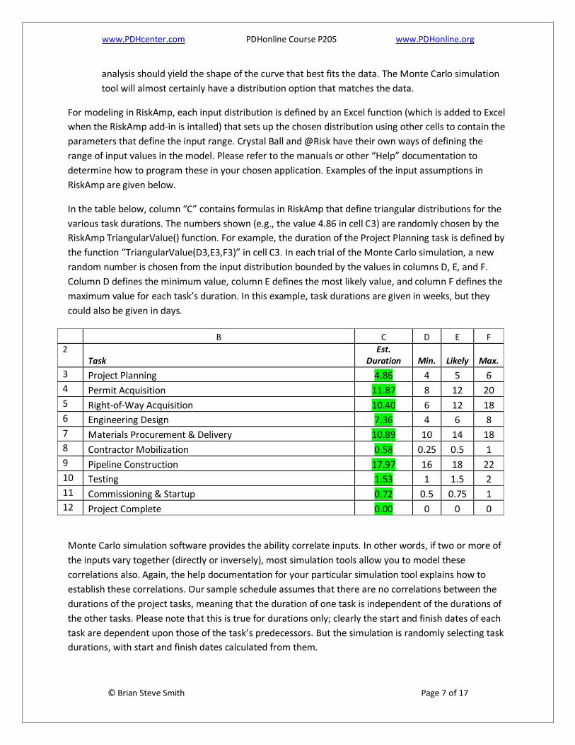
In the table below, column “C” contains formulas in RiskAmp that define triangular distributions for the

various task durations. The numbers shown (e.g., the value 4.86 in cell C3) are randomly chosen by the

RiskAmp TriangularValue() function. For example, the duration of the Project Planning task is defined by

the function “TriangularValue(D3,E3,F3)” in cell C3. In each trial of the Monte Carlo simulation, a new

random number is chosen from the input distribution bounded by the values in columns D, E, and F.

Column D defines the minimum value, column E defines the most likely value, and column F defines the

maximum value for each task’s duration. In this example, task durations are given in weeks, but they

could also be given in days.

B C D E F

2 Task

Est. Duration Min. Likely Max.

3 Project Planning 4.86 4 5 6

4 Permit Acquisition 11.87 8 12 20

5 Right-of-Way Acquisition 10.40 6 12 18

6 Engineering Design 7.36 4 6 8

7 Materials Procurement & Delivery 10.89 10 14 18

8 Contractor Mobilization 0.58 0.25 0.5 1

9 Pipeline Construction 17.97 16 18 22

10 Testing 1.53 1 1.5 2

11 Commissioning & Startup 0.72 0.5 0.75 1

12 Project Complete 0.00 0 0 0

Monte Carlo simulation software provides the ability correlate inputs. In other words, if two or more of

the inputs vary together (directly or inversely), most simulation tools allow you to model these

correlations also. Again, the help documentation for your particular simulation tool explains how to

establish these correlations. Our sample schedule assumes that there are no correlations between the

durations of the project tasks, meaning that the duration of one task is independent of the durations of

the other tasks. Please note that this is true for durations only; clearly the start and finish dates of each

task are dependent upon those of the task’s predecessors. But the simulation is randomly selecting task

durations, with start and finish dates calculated from them.





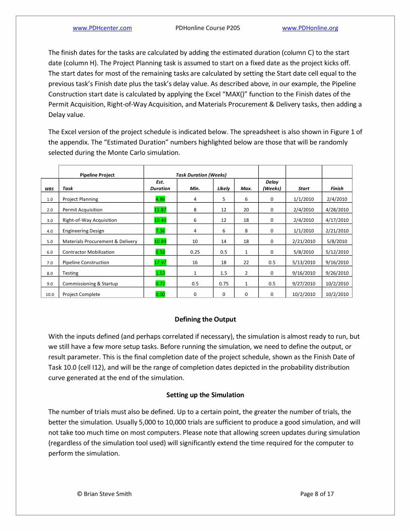
The finish dates for the tasks are calculated by adding the estimated duration (column C) to the start

date (column H). The Project Planning task is assumed to start on a fixed date as the project kicks off.

The start dates for most of the remaining tasks are calculated by setting the Start date cell equal to the

previous task’s Finish date plus the task’s delay value. As described above, in our example, the Pipeline

Construction start date is calculated by applying the Excel “MAX()” function to the Finish dates of the

Permit Acquisition, Right-of-Way Acquisition, and Materials Procurement & Delivery tasks, then adding a

Delay value.

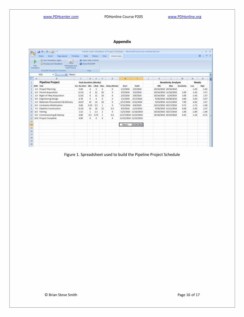
The Excel version of the project schedule is indicated below. The spreadsheet is also shown in Figure 1 of

the appendix. The “Estimated Duration” numbers highlighted below are those that will be randomly

selected during the Monte Carlo simulation.

Pipeline Project Task Duration (Weeks)

WBS Task Est.

Duration Min. Likely Max. Delay

(Weeks) Start Finish

1.0 Project Planning 4.86 4 5 6 0 1/1/2010 2/4/2010

2.0 Permit Acquisition 11.87 8 12 20 0 2/4/2010 4/28/2010

3.0 Right-of-Way Acquisition 10.40 6 12 18 0 2/4/2010 4/17/2010

4.0 Engineering Design 7.36 4 6 8 0 1/1/2010 2/21/2010

5.0 Materials Procurement & Delivery 10.89 10 14 18 0 2/21/2010 5/8/2010

6.0 Contractor Mobilization 0.58 0.25 0.5 1 0 5/8/2010 5/12/2010

7.0 Pipeline Construction 17.97 16 18 22 0.5 5/13/2010 9/16/2010

8.0 Testing 1.53 1 1.5 2 0 9/16/2010 9/26/2010

9.0 Commissioning & Startup 0.72 0.5 0.75 1 0.5 9/27/2010 10/2/2010

10.0 Project Complete 0.00 0 0 0 0 10/2/2010 10/2/2010

Defining the Output

With the inputs defined (and perhaps correlated if necessary), the simulation is almost ready to run, but

we still have a few more setup tasks. Before running the simulation, we need to define the output, or

result parameter. This is the final completion date of the project schedule, shown as the Finish Date of

Task 10.0 (cell I12), and will be the range of completion dates depicted in the probability distribution

curve generated at the end of the simulation.

Setting up the Simulation

The number of trials must also be defined. Up to a certain point, the greater the number of trials, the

better the simulation. Usually 5,000 to 10,000 trials are sufficient to produce a good simulation, and will

not take too much time on most computers. Please note that allowing screen updates during simulation

(regardless of the simulation tool used) will significantly extend the time required for the computer to

perform the simulation.





Some simulation tools may also require that a target range of cells be specified for the final statistical

analysis results to be presented. Again, refer to your specific program’s manual or help documentation.

With all of the input parameters defined, the output defined, and the simulation setup complete, we

can now run the simulation to obtain our results. As the simulation runs, the results of each trial are

collected by the computer. Upon completion of the simulation, the results are tabulated and graphed by

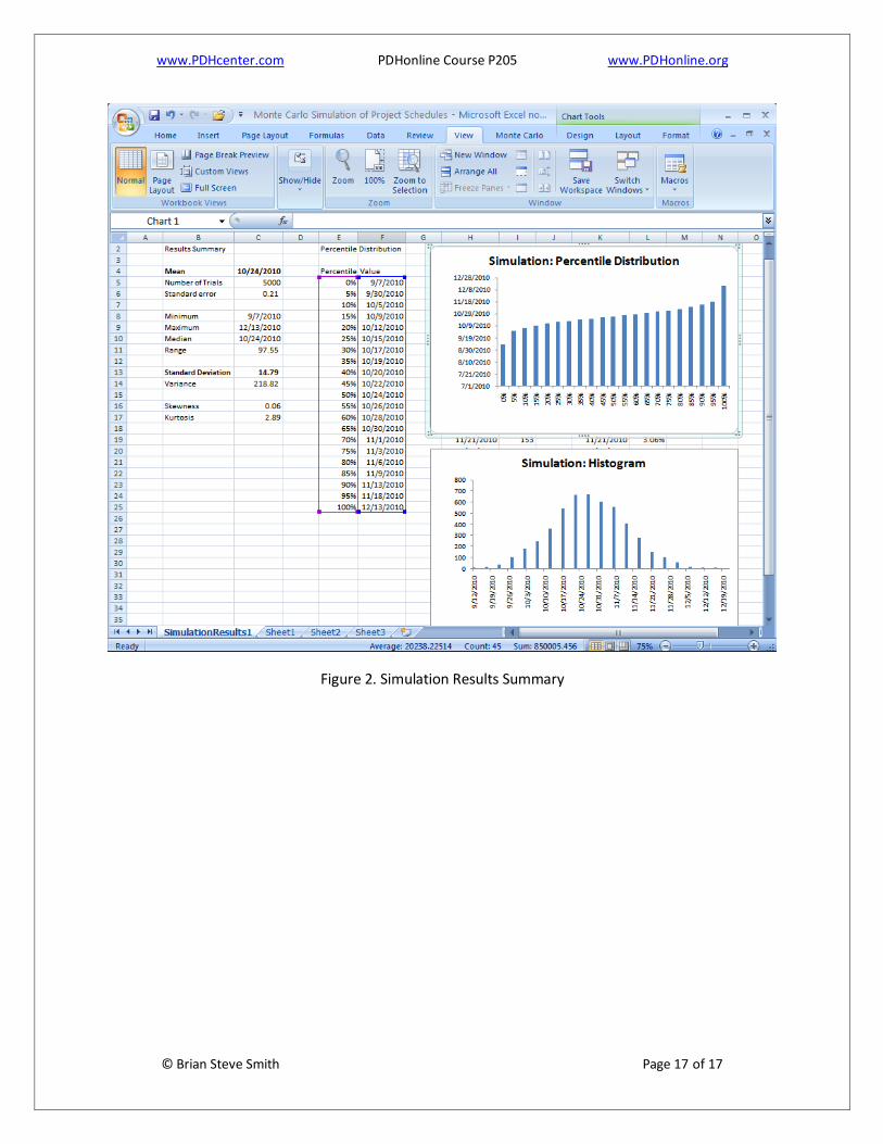
the simulation software. The full results of our simulation are shown in Figure 2 of the appendix.

Interpreting the Results

With the simulation complete and the output generated, the results must be interpreted for our project.

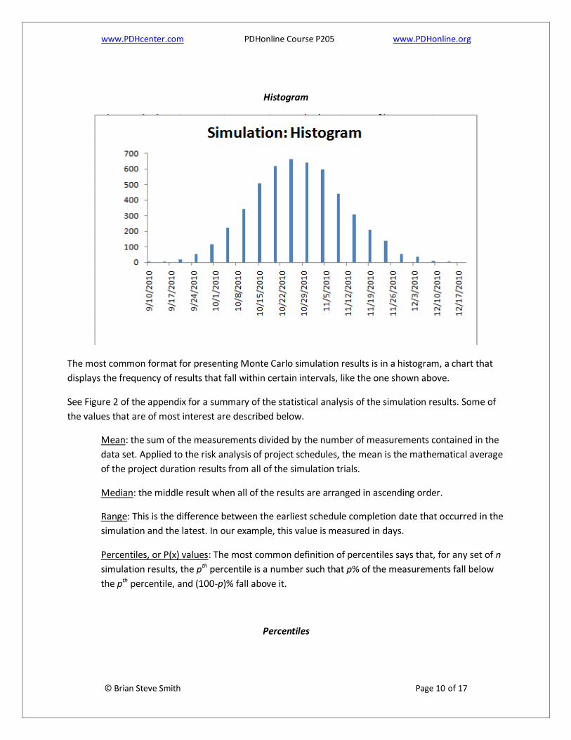
The most common output format is a histogram like the one shown above. This one shows that, for the

5,000 trials in our simulation, the resulting project completion dates follow a normal distribution along

the bell curve as shown.





Histogram

The most common format for presenting Monte Carlo simulation results is in a histogram, a chart that

displays the frequency of results that fall within certain intervals, like the one shown above.

See Figure 2 of the appendix for a summary of the statistical analysis of the simulation results. Some of

the values that are of most interest are described below.

Mean: the sum of the measurements divided by the number of measurements contained in the

data set. Applied to the risk analysis of project schedules, the mean is the mathematical average

of the project duration results from all of the simulation trials.

Median: the middle result when all of the results are arranged in ascending order.

Range: This is the difference between the earliest schedule completion date that occurred in the

simulation and the latest. In our example, this value is measured in days.

Percentiles, or P(x) values: The most common definition of percentiles says that, for any set of n

simulation results, the pth percentile is a number such that p% of the measurements fall below

the pth percentile, and (100-p)% fall above it.

Percentiles





The percentiles are usually of most interest to the project manager and stakeholders. These are the

completion dates that correspond to given probabilities. The numbers may be used two different ways.

Sometimes we refer to the “P10” value as the one for which a 10% probability exists of achieving or

beating it. It may also mean the value for which there is a 90% probability of achieving or beating it.

Some Monte Carlo simulation tools allow you to specify which convention you prefer. In our example,

the “P90” completion date is the one for which there is a 90% probability of achieving or exceeding it,

and corresponds to the 90th percentile in the table below.

Percentile Distribution

Percentile Value

0% 9/5/2010

5% 10/1/2010

10% 10/6/2010

15% 10/9/2010

20% 10/12/2010

25% 10/14/2010

30% 10/16/2010

35% 10/18/2010

40% 10/20/2010

45% 10/22/2010

50% 10/24/2010

55% 10/26/2010

60% 10/28/2010

65% 10/30/2010

70% 11/1/2010

75% 11/3/2010

80% 11/6/2010

85% 11/9/2010

90% 11/13/2010

95% 11/18/2010

100% 12/13/2010

This range can be useful when conveying schedule expectations to stakeholders. The stakeholder can

use the associated dates and probabilities to plan, and even though it might not give the results that all

stakeholders desire, the probability range conveys a consistent expectation of outcomes to all

stakeholders.

Another way of presenting the percentile results is in a graphical distribution, as shown below. The

information is the same as in the table, but sometimes reading the graph is more intuitive.





Sensitivity Analysis

Another helpful part of the risk analysis is called a “sensitivity analysis”. This task fixes all but one of the

inputs at their most likely values, then varies the remaining input from its minimum value to its

maximum value, noting the range of outputs that results. Each input is varied, one at a time, between its

minimum and maximum values, and a table is created of the range of project completion dates that

result for each individual task. This information is often presented either in a table of values (see below),

a “spider diagram,” or a “tornado diagram.” These diagrams are beyond the scope of this course, but

can be useful in understanding the results of the sensitivity analysis. Each of these is a different way of

depicting the same information. Depending on the simulation tool used, the sensitivity analysis may be

performed automatically or manually.

The value of the sensitivity analysis is that it shows, at a glance, which tasks the overall project

completion date is most sensitive to. When a project’s completion date is critical, the sensitivity analysis

helps the project manager and stakeholders determine to which tasks they should apply resources to

most effectively mitigate schedule risk. The results of the sensitivity analysis for our Pipeline Project are

shown below:





The graph above was produced manually by varying the durations of each task individually, and

recording the earliest project completion dates (from each task’s shortest duration) and latest

completion dates (from each task’s longest duration) in a table (below). For example, if the permit

application process takes 8 weeks (minimum task duration), and all other tasks are completed in their

most likely duration, the project completion date will be 10/14/2010. If the permit application process

takes 20 weeks (maximum task duration), and all other tasks are completed in their most likely duration,

the project completion date will be 11/18/2010. The table was then sorted and graphed using Excel’s

chart functions. Some Monte Carlo simulation tools perform this sensitivity analysis automatically.

Sensitivity Analysis

Task Early Project Comp. Date

Late Project Comp. Date Sensitivity (wks)

Project Planning 10/14/2010 10/14/2010 -

Permit Acquisition 10/14/2010 11/18/2010 5.00

Right-of-Way Acquisition 10/14/2010 11/4/2010 3.00

Engineering Design 9/30/2010 10/28/2010 4.00

Materials Procurement & Delivery 9/23/2010 11/11/2010 7.00

Contractor Mobilization 10/12/2010 10/17/2010 0.71

Pipeline Construction 9/30/2010 11/11/2010 6.00

Testing 10/10/2010 10/17/2010 1.00

Commissioning & Startup 10/16/2010 10/19/2010 0.43





This sensitivity analysis indicates that the project schedule is most sensitive to Materials Procurement &

Delivery, which can influence the completion date by +2.5 / -4.5 weeks, or a total sensitivity of 7 weeks.

The project’s second highest sensitivity is to Pipeline Construction, which can influence the completion

date by +2.5 / -3.5 weeks, or a total sensitivity of 6 weeks. Knowing that this is where the most schedule

sensitivity lies, we may decide to pay delivery premiums for materials, and perhaps pay for additional

overtime, etc., for the contractors to expedite construction.

Presentation of the Results

How to present these results depends on the audience, and the project manager’s expert judgment

again comes into play. It is not uncommon for these results to become the basis of a negotiation of

sorts, in which stakeholders may want to change the input assumptions and re-run the simulation for

other scenarios. This is a great application of Monte Carlo simulation, as it helps to create a better

understanding of the project schedule risks among all stakeholders, and highlights the tasks to which the

project schedule is most sensitive.

From the results of our Pipeline Project simulation, we conclude that our project is most likely to be

complete in late October, 2010, but could complete as early as early October 1 or as late as November

18 (ignoring the upper and lower 5th percentiles). The mean result of our simulation places our

completion date at October 24th, with a 50% percent probability of meeting or exceeding it. A

stakeholder may ask, “What date should I plan on the project being complete?” The answer may be

another question, “How much confidence do you need to have in that date?” Referring to the

percentiles, the stakeholders can make their own plans around completion dates, depending on the

degree of certainty needed in their planning.

The presentation of the results to the project stakeholders should always contain the following

information:

“Point case” schedule indicating all critical path tasks and dependencies

Monte Carlo Simulation Assumptions

o It is a good idea to provide a document summarizing the “risk ranges” applied to all

inputs.

Simulation results

o Histogram

o Table of percentiles

o Results of sensitivity analysis

The stakeholders should have the benefit of a clear understanding of the level of uncertainty included

for all of the tasks in the project schedule. This will facilitate a better mutual understanding of the





probable results, and give stakeholders the opportunity to challenge these assumptions, perhaps making

the next version of the analysis more realistic.

Ultimately, the decision of what to results to convey to which stakeholders is up to the project manager.

In general, conveying a probability-weighted range of project outcomes enables all stakeholders to

perform or manage their project tasks more effectively. For example, if the sales person who has regular

contact with the customer is given only one estimated completion date (i.e., a deterministic schedule),

and the project completion slips past this date, the customer may assume that the firm lacks the ability

to execute. However, if the sales person gives the customer a range of dates and probabilities (from the

risk analysis), the customer may be more likely to understand the uncertainties inherent in the project

schedule, and the analysis may improve credibility in the eyes of the customer.

Quantifying and understanding risks are the first steps toward managing them, and the ultimate

objective of using Monte Carlo simulation for project schedule analysis is better management of

schedule risk.





Appendix

Figure 1. Spreadsheet used to build the Pipeline Project Schedule





Figure 2. Simulation Results Summary



monte carlo simulation of project schedules - … meadow estates drive ... monte carlo simulation of...

Documents