Monte Carlo Simulation of the Potts Model in 2-5

Dimensions

Physics 271 Final Paper

Noah Kurinsky

March 13, 2015

Abstract

In this paper, I explore the behavior of the Potts model in the parameter space of spinnumber, lattice size, dimensionality, measuring critical behavior and comparing to the meanfield solution. I find that the Potts model exhibits rich behavior for all non-using cases andexhibits a striking symmetry across spin and dimension in terms of mean field applicability. Inaddition, I present fitted values for the critical exponents β and η at well as critical temperatureTc, and compare to predicted and previously measured values. I conclude discussing the successof my simulations and behavior of the model across the parameter space.

1 Introduction

Lattice theories represent an important probe of macroscopic properties of systems composed ofmicroscopic, quantum degrees of the freedom, as the simplest models are able to reproduce phasetransition behavior seen in complex macroscopic systems. The simplest model is that of the Isingmodel in two and three dimensions, which is a simple two-spin model symmetric in spin, whichshows a spontaneous symmetry breaking below a critical coupling value between spins, and ischaracterized by the hamiltonian

−βH = K∑〈ij〉

sisj + h∑i

si + g

where si, sj ∈ {−1, 1}, K is a dimensionless coupling constant related to dimensionless temperatureT as K = 1/T , h is external applied field, and g is simply set by choice of gauge. The partitionfunction Z = exp(−βH) is thus clearly optimized in the low temperature case by high alignmentbetween spins; the point at which this behavior disappears is a classic example of a phase transition.

The Ising model is an important model within the framework of statistical mechanics as ithas been shown to model ferromagnetic materials very well, and phenomenologically explain phasetransitions and critical behavior between magnetized and non-magnetized states [10]. The Isingmodel is also presented as the simplest example of a quantum statistical system, as the two-dimensional system is exactly solvable through a variety of techniques which cover a wide swatheof techniques in statistical mechanics [10, 3], while the higher dimensional models provide primeexamples of mean field theory and the lowest dimensional models provide basic illustrations ofspatial renormalization groups.

The wide influence of the Ising model motivates generalizations of the model beyond dimen-sionality, including to vector spins (the O(n) model), spins of varying energy (the s-spin model),and spins of equal energy which are nonetheless exclusive and tend to co-align. This last model hascome to be known as the “random-bond” model, or for historical purposes the Potts or Ashkin-Teller-Potts model [11], and is typically parameterized in terms of dimensionality d and number of

1

energy states q, with the hamiltonian

− βH = K∑〈ij〉

δσiσj + h∑i

σi + g (1)

where σi is a complex vector spaced rotationally equidistant in the complex plane:

σi = exp

(i2πsiq

), si = 1, 2, ..., q (2)

note that this reduces nicely to the Ising model for q = 2, giving spins of plus and minus one. Inaddition, spins are equally weighed, as opposed to the spin-s model where energy difference betweenspins is proportional to their separation, in the Potts model all spins are equally preferred startingfrom an unbiased state.

The Potts model does not have any immediately obvious applications, as the Ising model does,but it has proven useful for a variety of exotic processes as various values for q represent differentuniversality classes (they can be used to model systems with similar critical exponents) [11]. Thelarger amount of degrees of freedom in the Potts model allow connections to be drawn betweenspin systems with critical exponents which do not conform to those in the Ising model, such asbond percolation (q = 1), ordered absorbed monolayers (d = 2) and cubic ferromagnetic lattices inparticular field symmetries (d = 3, q = 3), to name a few [2, 4, 11].

On theoretical grounds, the Potts model allows us to further explore the transition in spin modelsystems between mean field (first order) and continuous (second order) phase transitions. Whilethe Ising model simply sets restrictions for our q = 2 cases, and proves that mean-field theory onlyapplies to spin-2 systems in hyper-dimensional (d > 3) systems, the Potts model can reveal systemswhich obey mean-field theory in 2 and 3 dimensions for q > 2, as we shall see later in this paper.

In this paper I explore the critical properties of the Potts model in detail for 2, 3, and 4dimensions through Monte Carlo simulation for q=2-5, 10, and 100, and show qualitatively thecritical behavior in 5 dimensional lattices for a subset of these spin values. In particular, I fitfor the critical exponents η and β, the critical temperature, and the corresponding connected-correlation length to show trends of correlation between sites as a function of spin, dimensionality,and temperature. One prediction of mean-field theory for the Ising model in this regard is a valueof 0 for η, thus the values obtained for η should provide some probe of this critical behavior on topof the order of the phase transition.

In section 2, I will describe the theoretical background of the model and describe the criticalexponents I will fit, as well as discuss the mean-field solution of the Potts model. In section 3, I willdiscuss the Monte Carlo techniques I employed to simulate the Potts model across this parameterspace, and briefly discuss practical considerations relevant time and computing constraints of thisproject, including convergence testing and optimization. In section 4, I will present the results ofmy numerical simulations and compare to theoretical expectations for the parameter space covered,and in section 5 will present my conclusions based on this comparison. The code and the majorityof the figures for the numerical simulation will be included in the appendix at the end of this paper.

2 Spin Systems and Lattice Theory

As discussed in the introduction, and at length in Kardar [10], Wu [11] and Binder and Heermann[3], discrete lattice models provide convenient, easy to implement, and easy to understand approxi-mations for simple systems which come with a wide variety of approximate and exact mathematicatools and solutions. In this section, I will describe the Potts model in more detail, discuss the mean

2

field solution and exact two-dimensional solutions, and discuss crucial similarities and differencesbetween the Potts and Ising models. The results of this section will be applied to fitting connectedcorrelations in section 4 and in drawing conclusions from the numerical simulations.

2.1 Potts Model

The Hamiltonian for the Potts model was given in equation 1, where it was stated to be a general-ization of Ising hamiltonian with a small caveat, which needs to be noted before discussing criticalproperties further. Note that the Ising system has spins si = ±1, which can parameterized as q=1and q=2 given that in a q = 2 system, equation 2 gives σ1 = −1 and σ2 = 1. In addition, we canparameterize their product in the hamiltonian from the introduction as

sisj = (2δσiσj − 1)

which gives the relation

−βH = KIsing

∑〈ij〉

(2δσiσj − 1) + hIsing∑i

σi + g = KPotts

∑〈ij〉

δσiσj + hPotts∑i

σi + g′

2KIsing

∑〈ij〉

δσiσj + hIsing∑i

σi + g −NKIsing = KPotts

∑〈ij〉

δσiσj + hPotts∑i

σi + g′

which immediately gives the relation

KPotts = 2KIsing or TPotts =1

2TIsing (3)

and the extra factor of KPotts gets absorbed into the gauge g’, which at a fixed temperature will notaffect the evolution of the system [11]. Thus the definition of the Potts model with this hamiltonianrequires that comparing dimensionless temperatures between models, we must halve standard Isingcritical temperatures to obtain the corresponding Potts temperatures.

We define the order parameter, which describes the average spin state in the system, as thevector mean of all individual spins [9]:

m = 〈s〉 =1

N

∣∣∣∣∣N∑i=1

exp

(i2πsiq

)∣∣∣∣∣ (4)

such that completely correlated states will evaluate to 1 and uncorrelated states to 0; the phasefactors from the uncorrelated states will cancel. In addition, the correlation between spins sisjaccording to the coupling in the hamiltonian can be written [11]

〈sisj〉 =q

q − 1

1

Np

Np∑si,sj

(δ(si − sj)−

1

q

)(5)

This follows as the simple sum of weighted probabilities. In a completely uncorrelated system,the probability of two spins having the same value is 1

q , and the correlation will be zero, and in acompletely correlated system the expectation of the delta function will be 1, and the value in thesum will evaluate to N q−1

q , giving the correlation a value of 1.

3

2.1.1 The Ising Limit

For q = 2, we expect to find that the Potts model will reduce to the Ising model, and this serves asa basic test of the generality of the model as well as the success of the Monte Carlo simulation andapplicability of the modified order parameter and correlation function. For q = 2, we find (withsi = {1, 2} and s′i = ±1 giving s′i = 2si − 3):

m = 〈s〉 =1

N

∣∣∣∣∣N∑i=1

exp (iπsi)

∣∣∣∣∣ =1

N

N∑i=1

(2si − 1) =1

N

N∑i=1

(2si − 3) =1

N

N∑i=1

s′i

〈sisj〉 =2

Np

Np∑si,sj

(δ(si − sj)−

1

2

)=

1

Np

Np∑si,sj

(2δ(si − sj)− 1) =1

Np

Np∑si,sj

s′is′j

which are the order parameter and spin correlation we calculate for the Ising model, confirmingthat these equations work properly in the Ising limit. Here, Np is number of probes, assuming theexpectation is taken over Np different points all separated by x = i − j in different areas of thelattice.

2.2 Mean Field Solution and Phase Transitions

In studying exact and approximate solutions to the Ising model in any of D dimensions, we foundthat mean field theory is only exact in four or more dimensions, and requires parameterizationin terms of critical exponents for systems with low spin numbers in 2 and 3 dimensions, buttransitions are either continuous or second order in temperature; there are no discontinuities in theorder parameter as a function of temperature.

Wu [11] lays out the derivation of mean field theory in the more general case for a system ofq spins in d dimensions; the derivation is short and quickly highlights the key difference betweenIsing and Potts model expressions for free energy. Starting from the mean field hamiltonian for thePotts model in terms of the ferromagnetic coupling ε > 0:

H = − 1

Nγε∑i<j

δ(σi, σj)

we let xi be the fraction of spins in state i (where i = 1, ...q) and all xi sum to one. This tells usthat the energy and entropy per spin are

E

N= −1

2γε∑i

x2i

S

N= −k

∑i

xi ln(xi)

which gives the free energy per spin A, with K = εβ, as

βA =∑i

(xi ln(xi)−1

2γKx2i )

and parameterizing this fraction in terms of the order parameter, for majority spin 1, as

x1 =1

q[1 + (q − 1)m], xi =

1

q(1−m), i = 2, ..., q

4

we find the expansion between m = 0 and small m 6= 0 has the form

β[A(m)−A(0)] =q − 1

2q(q − γK)m2 − 1

6(q − 1)(q − 2)m3 + ...

We find the preferred order parameter for a given temperature (remembering of course that K ∝1/T ) by minimizing this free energy, and note that this will always have a solution at s = 0, butfor sufficiently small temperatures we should be able to obtain other positive solutions of s0 whichminimize this equation. The key difference between the Ising and Potts cases here lies in the cubiccoefficient, which is zero for q = 2 and negative for q > 2, causing the magnitude of the coefficientto rise with increasing value of q. Wu [11] points out that the existence of this negative coefficientprevents the continuous behavior seen in the order parameter for q = 2 by preventing a small subsetof solutions from appearing until we observe a discontinuous jump in m from 0 to a finite value;this solution predicts that mean-field solutions for q > 2 have first order transitions.

This phase transition property is the primary behavior I intend to test through simulation, as itis the key feature of the Potts model which makes it distinct from the Ising model, which has onlycontinuous and second order transitions far from the thermodynamic limit [6]. Janke [9] mentionsthat most phase transitions which occur in nature are first order, which is most often identifiedthrough discontinuous changes in their order parameter as a function of temperature (e.g. statechanges between liquid and gas, etc). The Ising model is successful for ferromagnetic systems whichhave second order transitions, but this suggests the Potts model may be more ideal for systemswith many more degrees of freedom which can be seen to exhibit this characteristic. Janke [9] andBinder [2] also note that length and energy scales in the system will have differing behavior inthese types of transitions; for second order transitions these scales will diverge, but for first ordertransitions they will be merely discontinuous due to a finite but convergent asymmetric increase.

While the mean field solutions provide predictions for the higher dimensional lattices, the exactsolutions for the Potts model on a 2-D lattice (in arbitrary geometries) comes from equivalence toan ice-rule vertex model, and we can obtain the exact solution for the critical temperature [11]:

Tc = [ln (1 +√q)]−1 (6)

which is remarkably uncomplicated, and will be easily testable through monte carlo simulation.Beyond two dimensions there are no exact solutions, as in the Ising model, but due to the largeparameter space of the Potts model even less is completely determined given the large number ofchoice for spin and the different applications they have. Numerical predictions from other works,contained in the review by Wu [11], are included in table 1 for comparison to my numerical values.

2.3 Correlation Length and Critical Exponents

In addition to phase transition properties, we would also like to compute some of the criticalexponents for various Potts models. Critical exponents are scaling relations of given characteristicsas power laws in temperature, and are mostly valid near the critical point [10]. I am concerningmyself primarily with correlation length and behavior of the order parameter near the criticalpoint, as these behaviors are tied to behavior of systems near phase transition and should showsimilar variation about the critical point. The first critical exponent I’d like to measure is β, whichcharacterizes the behavior of the order parameter near the critical point as the power law

m =

∣∣∣∣Tc − TTc

∣∣∣∣β (7)

5

Given that the order parameter runs between 0 and 1 this is obvious not a valid expression morethan a few fractions of the critical exponent away, but describes generally the sharpness with whichthe phase transition occurs, before the onset of any first order discontinuities.

The second critical exponent I will measure is related to the mean-field solution for the connectedcorrelation function. The calculation of equations 4 and 5 numerically allows us to compute theconnected correlation function

g(r) = 〈s0sr〉 − 〈s0〉〈sr〉 = 〈s0sr〉 −m2 (8)

which we can then use to determine correlation length in the lattice as a function of temperatureas well as the critical exponent η, given the canonical scaling relation [10]

g(r) ≈ 1

rd−2+ηexp

(−rξ

)(9)

One of the primary predictions of the mean field theory solution to the Ising model, which shouldhold for at least q = 2, is that there exists a space of models of q = 2 for which η is definitely non-zero, where transitions are second order, and a space where η is 0 and transitions are first order. Theprimary numerical estimates from the following Monte Carlo simulations will be estimates of relativecorrelation length across different values for q, estimates of η for a given d and q, and estimates ofthe critical temperature for each model; the former two measurements will be obtained primarilythrough a least-squares fit to a function of the form of equation 9 with a floating normalization. Itshould be noted that this equation will only strictly apply in the large x limit, though on a smallfinite lattice it will provide a reasonable approximation for all but r = 0.

3 Monte Carlo Methods

Monte Carlo methods describe a set of techniques employed to simulate stochastic systems andevaluate complex relationships without exhaustively testing every microstate of a given system. Inthe context of lattice models, Monte Carlo simulations encompass a set of rules for evolving thelattice through time in a manner which accurately and efficiently predicts the equilibrium behaviorof the lattice for a given point in state space. A key characteristic of a Monte Carlo chain, or setof sequential lattices in this case, is that each individual macrostate for which measurements areconducted during the course of the simulation be completely uncorrelated with any state aside fromthe one immediately preceding it. In this way, we ensure that we can estimate mean quantitiesusing the relation

〈X〉 =2

N

N∑i=N/2

Xi

without folding in correlations which may bias the measurement. For it to be a true expectationvalue, each lattice must represent a distinct possible macro state. In the above equation, we sumover the latter half of the samples to remove the effects of initial conditions on the final answer,giving the simulation time to ”thermalize”.

The general structure of a Monte Carlo algorithm is as follows

• Generate random proposed change to current state

• Accept new state based on physically motivated prescription

• Update state

6

• Repeat until convergence

The most general lattice implementation of this procedure is the Metropolis algorithm (describedin Binder and Heermann [3] and Kardar [10]) which randomly selects a spin to change, accepts thechange if it reduces the free energy of the system, or conditionally accepts the change to a higherenergy by a Boltzmann factor, with the energy argument the difference between the flipped andnon-flipped energy states. This is a good illustration of the idea of Monte Carlo simulation, butwhen confronted with critical behavior its performance suffers. In this section I will describe theupdate rule I employed, the Wolf clustering algorithm, as well as my convergence testing and otherkey implementation details, including the parameter space I sampled and the limitations of mysimulation due to computing constraints.

3.1 Wolf Clustering Algorithm

Clustering algorithms entail flipping large groups of spins simultaneously, such that in the criticallimit whole clusters can be flipped quickly as opposed to relying on random reassignment of adjacentsites which should be largely correlation. Baillie [1] compared the performance of the Wolf andSwendson-Wang algorithm for the two-dimensional Potts model, finding that the Wolf algorithmconverges much more quickly (measured as an autocorrelation timescale) across many different spinvalues, and thus I chose to implement this clustering algorithm for my Monte Carlo simulation.

We obtain the Wolf algorithm by rewriting the partition function in a similar manner to Janke[9], but modified for the Potts model:

Z =∑{σi}

exp (−βH)

=∑{σi}

exp

K∑〈ij〉

δ(si − sj)

=∑{σi}

∏〈ij〉

eK ((1− p) + pδ(si − sj))

=∑{σi}

∑{nij}

∏〈ij〉

eK((1− p)δnij ,0 + pδ(si − sj)δnij ,1

)where

p = 1− e−K

and nij is 0 for inactive bonds and 1 for active bonds. This effectively parameterizes the partitionfunction in terms of clusters, which leads directly to the simulation algorithm [1, 2, 3, 9]:

1. Choose random seed site, flip spin to random new spin

2. Check all neighboring spins, and if their spin matches the original seed spin, add to clusterwith probability p

3. If added to cluster, flip to new spin and check that spin’s neighbors

4. Step is complete once all spins have been checked

5. Repeat until convergence

7

They key difference between this and the Ising derivation is that the coupling constant in this casedoes not have a 2 in front, but given that this should produce identical behavior to the Ising modelin the q = 2 limit, we see from equation 3 that

p = 1− e−KPotts = 1− e−2KIsing

and so this still reduces to identical behavior in the Ising limit. The key difference here is that inthe Ising case, the choice of new cluster spin is obvious, but in the Potts case, the additional stepof randomly choosing a new spin must be taken.

3.2 Simulation Methodology

I implemented the above algorithm to simulate the individual steps in the Potts model, addingin additional considerations based on properties of Monte Carlo steps. My general simulationprocedure was the following:

1. Initialize 3-5 independent lattices, setting spins randomly

2. Run each lattice blindly for 10 Monte Carlo steps, to generate an initial thermalization

3. Run each lattice for 1 Monte Carlo step

4. Compute current Monte Carlo averages for magnetization and correlation

5. Check for convergence

6. If converged, print and exit, otherwise repeat from step 3 if below maximum iteration limit

Following the example of Binder and Heermann [3], we can define a Monte Carlo step as approx-imately N spin flips, where N is the number of spins in the lattice. In practice, I implementedthe cluster flip method to loop until a given number of flips have occurred, and but by computingN = Ld at the beginning of the run and passing this as the limit to these functions, running asingle step is a single line of code in my main function (L being lattice side length and d beingdimension).

3.2.1 Convergence

Testing for convergence amounts to determining when the measureables resulting from the simula-tion have stabilized in time. The two schools of thought in convergence testing amount to running along, detailed simulation and determining convergence based on the autocorrelation of the measure-ment (as in Dunkley et al. [7]), or running multiple parallel simulations and comparing independentresults as the simulations progress until they have stabilized close enough to each other [5]. Giventhat the mean magnetization and connected correlation values should converge to stable values,I opted for the second method, and chose to run a few separate chains in parallel to determineconvergence.

The most basic convergence criterion is to require all measureables to lie within a predeterminedfraction, such that parameter estimates can thus be assumed to be accurate to the order of thisrequirement. The formulaic representation of this method would resemble

(max({µ})−min({µ})/(domain(µ)) < threshold

where {µ} is an array of the mean value of the parameter for each of the independent lattices, anddomain represents the accepted range of the parameter; this then reduces to relative error within a

8

given domain. For the parameters in this model, all domains are 0-1 and thus the denominator istrivially 1. In practice, I required all variables to be simultaneously converged for full convergenceto be reached, and included a maximum run limit as a contingency end criterion, as in the previoussection, and my nominal convergence threshold was 0.01 (which sets the scale for most of mymeasurement errors, but was necessitated by runtime considerations).

This formula of course assumes stochastic deviations will be distributed about the true mean,and that chains will settle to the mean from all directions, but in practice it fared well in producinga very continuous and well-behaved value for magnetization as well as the larger of the connectedcorrelation points. In theory, what is being tested is that the expectation value of each parameterreaches a stable value regardless of initial condition; this is the motivation for using multipleindependent realizations of the lattice. More advanced convergence tests would require each valueto converge to a fraction of the mean, but the run-time required for far away connected correlationvalues to reach this point was prohibitive, so the simpler criterion was used to allow more reasonableconvergence times.

3.2.2 Implementation

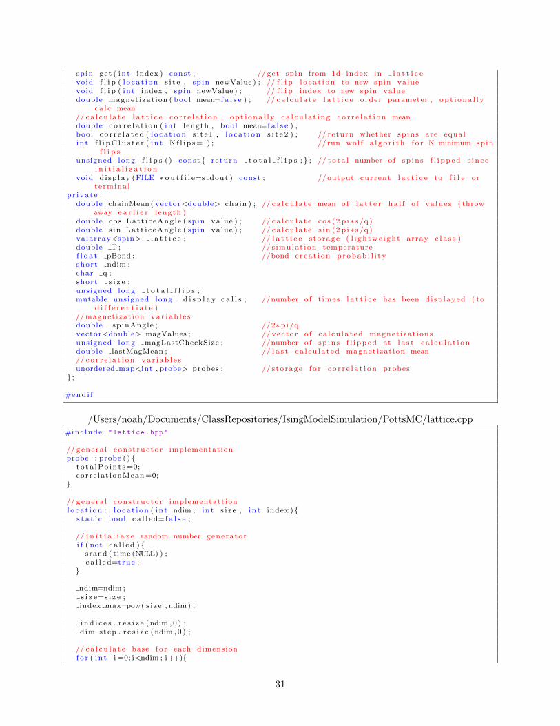
The C++ code used to perform the Potts model simulations is shown in Appendix B. I decidedto implement the simulation in C++ due to past experience using higher level languages to per-form Monte Carlo simulations, where I saw a loss of ability to optimize performance. Some of thekey features which decreased runtime and memory usage were including lookup tables for complexoperations whenever possible (such as computing sine/cosine values and array indices from mul-tidimensional coordinates) and representing each spin by a character (one byte of memory, range0-255) within an array. I mapped indices instead of mapping spins to vectors due to the ease withwhich arrays can be accessed and locations stored for iteration and random searches (included inthe clustering algorithm and calculation of parameters).

Within the program, I computed order parameter by simply summing across all components.Given that sampling every lattice site at every iteration for correlation would be overkill, I thengenerated a subset of up to 1000 points (limited to 1/4 of the lattice size), each of which servedas the zero point for d probes (one per dimension) a distance r from the zero point. By averagingover this subset of points at each Monte Carlo step, I balance efficiency with statistical robustnessagainst fluctuations. when computing correlation, for which considering each point is expensiveand prone to bias. In addition, correlation values for r between 1 and 10 were calculated, exceptin the case that L/2 was less than 10, a which point calculations were limited to this value. Thelocations of these probes were stable in time, stored through a lookup table indexed by requestedcorrelation length r.

For more details, see Appendix B.

3.2.3 Parameter Space Sampling

The effective model space for these simulations is three dimensional, including lattice size, dimen-sion, and spin number q. I wanted to sample the space of d = 2 − 5 and q = 2 − 100, as well asa reasonable sampling of lattice size. I decided to aim for each lattice of contain ∼ 106 elements,based on initial simulations which set this as the maximum size for which my code converged ina reasonable amount of time (approximately 4-6 hours on the SLAC batch). This left me withample room to explore lattice size effects in two and three dimensions, while being able to obtainreasonable results for phase transitions and critical exponents across all dimensions and the spins2,3,4,5,10, and 100 (although 100 did not converge in higher dimensional cases).

9

I employed the SLAC batch farm to submit small ranges of temperatures in parallel and a largegrid of the parameter space, allowing me to collect data resolved to 0.01 in temperature for allmodels. The size of the largest lattices, used to compute critical exponents, can be seen in the firstcolumn of table 1, and the parameter space sampled can be seen in the first two columns of thesame table.

3.3 Parameter Fitting

Once simulations were completed, I obtained data files of connected correlation values, magneti-zations, and associated errors on each from variance across lattices. I employed Python for myplotting and function fitting, using a least-squares minimization routine for parameter fitting andinitial uncertainty estimation. The true uncertainty is, as always the combination of systematic andstatistical uncertainty, and for most of the lattices the statistical uncertainty was limited by theconvergence criterion, which was the quoted error value for parameters which the curve_fit rou-tine thought we higher confidence. The code used for all parameter fitting can be seen in AppendixC.

In addition, fits could not be obtained for all models, most notably the q = 100 case due tolow statistics and sharp first order transitions, so a variety of measurements of Tc were made toobtain the true value, including the value resulting from the fit for β and the point of maximumcorrelation and correlation length, resulting in between 1 and 3 high confidence estimators forcritical temperature. The order of phase transitions was judged based on 1) the sharpness of thetransition, 2) the one-sidedness of the correlation length versus temperature curve, and 3) thedivergence of correlation length as a function of temperature. Discontinuous transitions in orderparameter are immediately classified as first order, highly one sided correlation fits as well, andhighly divergent correlation functions are considered second order. Continuous transitions resemblea sloping curve which does not go to a step function in the thermodynamic limit.

4 Results

The full results of simulating all points in the dq parameter space can be seen in Appendix A. ThereI show order parameter as a function of size, temperature, dimension, and q for all points in theparameter space, and have over-plot the fits for β. I have also shown how lattice size contributesto overall convergence length; finite size naturally reduces correlation length as fewer sites producemore stochastic fluctuations due to weaker overall coupling. I have also included plots of orderparameter and connected correlation values for all models with the largest lattice size for comparisonof trends across the parameter space; it is interesting to note that as dimension increases, in generalcritical temperature increases, critical behavior becomes sharper, and correlation is greatly reduced.Also keeping in mind that all values are only confident to 0.01, it becomes obvious why fits in 4and 5 dimensions are highly error ridden, and they are relatively imprecise beyond r = 1. Table1 shows all successfully fitted values with theoretically or numerically predicted values from theliterature for comparison where available.

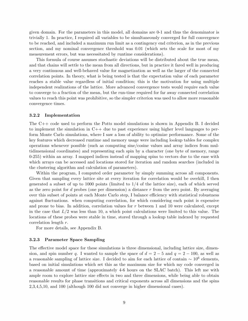
In table 1, the first point to discuss is the degree to which my measured critical temperaturesmatch predicted values. The accuracy of my values in two dimensions can be stated as a testamentto true critical nature of the model, as independent of lattice size the critical behavior in temperatureis fairly stable. The trend of temperatures versus dimensionality and spin is plotted in figure1, where the trend of lower critical temperature of higher spin and increasing temperature withdimensionality is apparent. We can attribute the first effect to the cause of critical temperature,relating it back to the mean field model, where we see that critical behavior occurs when spins

10

Figure 1: Critical Temperature Trends in q-d space

have clustered enough that one spins can become the majority spin by a significant fraction; thisfraction doesn’t need to be as large for lattices with more spins, and the free energy of these smallerclusters is easier to break, thus critical transitions occur at lower temperatures. In addition, higherdimensionality means more interaction between spins and systems of clusters with much largerenergies which are harder to break, contributing to higher critical temperature. In q > 2 systemsthis is also seen in the magnitude of the cubic term, which pushes critical transitions to lowertemperatures by removing higher temperature solutions above zero. Examples of critical and pastcritical lattices can also be seen in the appendix, where it is clear that typical clusters are muchsmaller at the critical point, and the system is relatively disordered already as judged by eye; thisis due to the large freedom in spin number and disorder comes about fairly naturally.

The phase transition behavior is also interesting to compare to mean field predictions, and theorder of transitions can be seen either in the figures in the appendix, the summary table, or theoverall summary in figure 2. Looking first at the bottom line (q = 2), we see that the observedbehavior is identical to expectations, namely that we see a transition to mean field behavior beyondd = 3. What is striking to note is the line which separates the region of second order and firstorder transitions is roughly symmetric about the unity line and intersects the points q = 2, d = 4and q = 4, d = 2, as seen in Wu [11], Binder and Heermann [3]. We see strikingly discontinuousfirst order transitions both in large q and large d, as expected, leading to a general observationthat more independent (non-interacting) degrees of freedom in a system will contribute to a morediscontinuous and lower energy phase transition. As noted in much of the literature, most naturalphase transitions are highly discontinuous, and this plot would suggest that this is natural if weassume most systems have more than two independent degrees of freedom. In this case, we canview the Ising model more as a peculiarity of the nature of magnetism, and view the Potts modelas a first step towards a general phase transition model.

11

Figure 2: Phase transition order in q-d space

4.1 Critical Exponents

Also included in table 1 are the values for critical exponents corresponding to the fits shown inthe appendix. The first note is that the Ising critical exponents are mostly in agreement withpredictions, though not good agreement. While critical temperature seems to behave well indepen-dent of all but the smallest lattice sizes, critical exponents appeared very size dependent, whichposed a challenge due to the runtime roughly scaling as lattice size to the power of dimensionality.The fit quality can be seen to decrease rapidly in proportion to linear grid size, despite the gridshaving the same order of magnitude total grid sites. Size effects are very prominent in Monte Carlosimulations, and many of the literature focus on only one or two points in this parameter space toget much better converged data with higher precision to better estimate a few critical parameters(as in Herrmann [8]. It was noticeable, during simulation, that runtime increased with lattice size,spin number, and dimensionality, reflective of the fact that the lattices were more resistant to con-vergence in these regimes. This is corroborated by the larger errors associated with increases inany of these three degrees of freedom.

Despite the large error bars, some trends are worth noting in these critical exponents. My fitsconfirm that correlation length does deviate from the mean field expectation in two dimensionsfor the Ising model, and suggests that simulation is consistent with expectation of near-mean-fieldand mean-field behavior in higher dimensions. In addition, there is a noticeable decrease in β as afunction of spin, and an increase as a function of dimension. This is reflective of sharper transitionsas a function of increasing spin, but less sharp in increasing dimension, suggesting more tension ina more coupled system and more resistance to phase transitions in higher dimensions and for lowerspin values, corresponding to a stronger coupling, which intuitively makes sense. It is hard to drawmany conclusions from my largely unsuccessful attempts to constrain η in higher dimensions, butit is notable that I could not find literature to compare η to, suggesting it is not a particularlymeaningful measurement. This makes sense given that high dimensional lattices, in general, willnot have high correlation between sites except near the critical point, where η has a less meaningfulimpact than it does in two dimensions, where is can deviate the power law from nominally non-existent. It is also easy to see that measuring it in 5 dimensions from my data would not provide

12

meaningful results, as the signal to noise ratio is of order unity.

d (size) q Order Tc,m βm ηm Tc β η

2 (1000) 2 2nd 1.13 ± .01 0.129 ± .02 0.29 ± .02 1.13 0.125 0.253 2nd 0.99 ± .01 0.088 ± .01 0.31 ± .04 0.99 0.111 0.274 1st 0.91 ± .01 0.071 ± .01 0.38 ± .04 0.91 0.083 0.55 1st 0.85 ± .01 0.068 ± .02 0.42 ± .04 0.85 0.083 0.510 1st 0.71 ± .05 0.48 ± .10 0.70 0.083 0.5100 1st 0.40 ± .05 0.42 0.083 0.5

3 (100) 2 2nd∗ 2.26 ± .01 0.25 ± .10 0.00 ± .10 2.30 0.327 0.0633 1st∗ 1.82 ± .01 0.15 ± .01 0.00 ± .15 1.82 0.174 1st 1.59 ± .015 0.11 ± .01 0.01 ± .20 1.545 1st 1.45 ± .01 0.085 ± .01 0.22 ± 1.010 1st 1.09 ± .05 0.06 ± .10

4 (64) 2 0 3.27 ± .01 0.45 ± .05 0.075 ± 0.3 3.32 0.5 03 1st 2.57 ± .01 0.18 ± .01 -0.82 ± 1.5 2.594 1st 2.21 ± .01 0.13 ± .03 0.57 ± 1.8 2.095 1st 2.00 ± .01 0.05 ± .10 -0.68 ± 2.010 1st 1.39 ± .02

5 (10) 2 0 4.30 ± .10 0.47 ± .02 4.41 0.5 03 1st 3.25 ± .05 0.18 ± .014 1st 2.60 ± .05 0.14 ± .15 2.575 1st 2.28 ± .0510 1st 1.54 ± .05

Table 1: Results of monte carlo estimates for critical temperature and critical exponent for the con-nected correlation function, which determines relative scaling of correlation in the lattice. Predictedvalues are taken from Binder [2], Wu [11], and Herrmann [8]. Errors on temperatures are estimatedbased on temperature sampling of 0.01 in simulations (despite fit errors being much lower), anderrors are quoted at the 5σ level. Blank spaces denote parameters for which high quality fits couldnot be ascertained. Note that predicted values will be those that the critical exponent convergesto for infinite lattice extent, so the functional value will be expected to disagree to some extentfrom the thermodynamic limit, with the effect increasing as a function of spin, given the stochas-tic nature of the simulation and no coupling between different spin values. Zeroth order denotescontinuous transitions.

5 Conclusion

The Potts model has proven interesting to simulate, and given its wide applicability to many naturalsystems, and the close connection of discontinuous order transitions to natural phase transitions, itis surprising that it has not drawn more attention in the literature. We have seen in this discussionthat the Potts model provides a more general probe of methods such as mean field theory andof relationships between quantum mechanical objects with more general properties, and that itencompasses the special case of Ising systems, which exhibit exotic properties different from themajority of Potts models. In addition, trends across a higher dimensional parameter space allowus to gain more insight into the ising model, which has provided solutions for many interestingreal systems. The transition between mean field and first order behavior also exhibits a symmetry

13

which is suggestive of a deeper mathematical framework behind the model, and these simulationshave convinced me of much theoretical ground yet to be made in what might be a fruitful area ofstatistical mechanics.

In addition, in comparison to the Metropolis algorithm the clustering algorithm provided a re-markably efficient means for computing a wide range of models without encountering an appreciableslow-down near the critical temperature. This feature of the monte Carlo simulation performedwell, but in retrospect much of the results I have presented were highly limited by error due tothe type of convergence criterion I implemented. An alternative method for measuring conver-gence is through the autocorrelation of a single simulation, and I think that method of convergencemay have allowed me to reach a greater degree of precision through less memory usage and fewercomputations per Monte Carlo step.

Despite the weakness of some of my measurements, they represent a much larger space ofmeasurements than I encountered in the literature, and I have presented trends in my parameterspace which in their entirety do not exist in the literature. This is a testament more to advances incomputing power since the last spurt of interest in the Potts model (most of the papers I cite datefrom the 1980s and employ cray supercomputers for comparable work), but I feel I have mappedout real and interesting behavior which could potentially describe the variety and variation ofphase transitions which occur in nature. I found the Potts model to be incredibly rich and capabledescribing a much wider swathe of behaviors than the comparatively specific and derivative Isingmodel, though exact solutions are less readily available and immediately transparent.

References

[1] Clive F. Baillie. Comparison of cluster algorithms for two-dimensional potts models. PhysicalReview B, 43(13):10617–10621, 1991. doi: 10.1103/PhysRevB.43.10617.

[2] K Binder. Static and dynamic critical phenomena of the two-dimensionalq-state potts model.Journal of Statistical Physics, 24(1):69–86, 1981.

[3] K. Binder and D. Heermann. Monte Carlo Simulation in Statistical Physics: An Introduction.Graduate Texts in Physics. Springer-Verlag, 2010. ISBN 9783642031632. URL https://

books.google.com/books?id=y6oDME582TEC.

[4] H.W.J Blate and M.P Nightingale. Critical behaviour of the two-dimensional potts modelwith a continuous number of states; a finite size scaling analysis. Physica A: Statistical Me-chanics and its Applications, 112(3):405 – 465, 1982. ISSN 0378-4371. doi: http://dx.doi.org/10.1016/0378-4371(82)90187-X. URL http://www.sciencedirect.com/science/article/

pii/037843718290187X.

[5] Stephen P. Brooks and Andrew Gelman. General methods for monitoring convergence of iter-ative simulations. Journal of Computational and Graphical Statistics, 7(4):434–455, 1998. doi:10.1080/10618600.1998.10474787. URL http://www.tandfonline.com/doi/abs/10.1080/

10618600.1998.10474787.

[6] S. Chen. Monte carlo simulation of phase transitions in a two-dimensional random-bond pottsmodel. Physical Review E, 52(2):1377–1386, 1995. doi: 10.1103/PhysRevE.52.1377.

[7] Joanna Dunkley, Martin Bucher, Pedro G. Ferreira, Kavilan Moodley, and Constantinos Sko-rdis. Fast and reliable mcmc for cosmological parameter estimation. Monthly Notices of

14

the Royal Astronomical Society, 356:925–936, 2005. URL http://arxiv.org/abs/astro-ph/

0405462.

[8] HJ Herrmann. Monte carlo simulation of the three-dimensional potts model. Zeitschrift furPhysik B Condensed Matter, 35(2):171–175, 1979.

[9] Wolfhard Janke. Monte carlo simulations of spin systems. In Computational Physics, pages10–43. Springer, 1996.

[10] M. Kardar. Statistical Physics of Fields. Cambridge University Press, 2007. ISBN9780521873413. URL https://books.google.com/books?id=nTxBhGX01P4C.

[11] F. Y. Wu. The potts model. Rev. Mod. Phys., 54:235–268, Jan 1982. doi: 10.1103/RevModPhys.54.235. URL http://link.aps.org/doi/10.1103/RevModPhys.54.235.

15

A Supporting Simulation Results

Figure 3: Lattice visualizations in 2D (100 sites per side) of q-3 and q-10 lattices in disordered andcritical states, showing how adding spins changes the appearance of critically ordered lattices.

16

Figure 4: Plots for all lattices of order parameter versus temperature for largest size lattice. Notethe sharp discontinuities in higher spins and higher dimensions, and the difference between the d2q=2 transition and the transitions at higher order, as well as the difference between the d=2 q=3transition and the other q=3 transitions (it is, just barely, continuous; there is a slope and it doesnot go directly to 0). This is a significant effect, as it was seen for all lattices, and what it plottedis a lattice 1000 sites per side.

17

Figure 5: Plots for all lattices of correlation length versus temperature for largest size lattice. Notethe difference between the two spin two and greater spin cases, which show marked one sidednesswith increasing significance going to higher dimensions or larger number of spin states. In addition,one can see how, for the 2 spin system, there are no discontinuities, and for higher dimension thisbecomes a move smooth function with less tendency toward divergence.

18

0.0 0.5 1.0 1.5 2.0 2.5

Potts Temperature

0.0

0.2

0.4

0.6

0.8

1.0

1.2M

agneti

zati

on

Spin Q=2

Size

10.0

24.0

32.0

48.0

64.0

100.0

1000.0

Critical Exponent Fit

0.0 0.5 1.0 1.5 2.0 2.5

Potts Temperature

0.0

0.2

0.4

0.6

0.8

1.0

1.2

Magneti

zati

on

Spin Q=3

Size

10.0

24.0

32.0

48.0

64.0

100.0

1000.0

Critical Exponent Fit

0.0 0.5 1.0 1.5 2.0 2.5

Potts Temperature

0.0

0.2

0.4

0.6

0.8

1.0

1.2

Magneti

zati

on

Spin Q=4

Size

10.0

24.0

32.0

48.0

64.0

100.0

1000.0

Critical Exponent Fit

0.0 0.5 1.0 1.5 2.0 2.5

Potts Temperature

0.0

0.2

0.4

0.6

0.8

1.0

1.2

Magneti

zati

on

Spin Q=5

Size

10.0

24.0

32.0

48.0

64.0

100.0

1000.0

Critical Exponent Fit

0.0 0.5 1.0 1.5 2.0 2.5

Potts Temperature

0.0

0.2

0.4

0.6

0.8

1.0

1.2

Magneti

zati

on

Spin Q=10

Size

10.0

24.0

32.0

48.0

64.0

100.0

1000.0

0.0 0.5 1.0 1.5 2.0 2.5

Potts Temperature

0.0

0.2

0.4

0.6

0.8

1.0

1.2

Magneti

zati

on

Spin Q=100

Size

10.0

24.0

32.0

48.0

64.0

100.0

1000.0

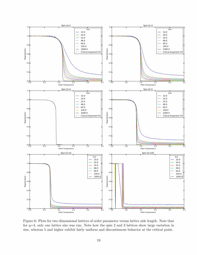
Figure 6: Plots for two dimensional lattices of order parameter versus lattice side length. Note thatfor q=4, only one lattice size was run. Note how the spin 2 and 3 lattices show large variation insize, whereas 5 and higher exhibit fairly uniform and discontinuous behavior at the critical point.

19

Figure 7: Plots for two dimensional lattices of fitted correlation length versus lattice side lengthand temperature, for some of the spins. Note that for q=4, only one lattice size was run. Note howq=2 and q=3 are tending towards divergence whereas higher spins have stable magnitudes in time,the hallmark of the difference between first and second order transitions, as discussed in the text.

20

Figure 8: Plots for three dimensional lattices of order parameter versus lattice side length. Notethat for q=4, only one lattice size was run. Again note the marked discontinuous behavior of allbut q-2, which has critical exponent fit down to 0, while other lattices do not.

21

Figure 9: Plots for four dimensional lattices of order parameter versus lattice side length. Againnote the marked discontinuous behavior of all but q-2, which has critical exponent fit down to 0,while other lattices do not.

22

Figure 10: Plots for five dimensional lattices of order parameter versus lattice side length. Againnote the marked discontinuous behavior of all but q-2, which has critical exponent fit down to 0,while other lattices do not.

23

Figure 11: Measurements of η and Tc. Here we can see that connected correlation does havedifferent power law dependence in difference dimensions, and tends to 0 much quicker than anexponential in 3 and 4 dimensions. Note also that the scale for the last plot is much narrower inx due to values being 0 for the remainder of the distance (an artifact of my convergence conditionbut indicative of nearly zero correlation), showing the even steeper fall to 0 than in 3 dimensions.

24

Figure 12: Measurements of correlation length versus q and temperature. The first plot is wellsampled and shows the behavior discussed earlier in this appendix, while the next two plots showroughly the same phase transition behavior but are highly noise limited, explaining the limitedfitting power in this dimensions for η.

25

B PottsMC (Simulation Code)

My simulation code for Potts models for arbitrary q levels, n dimensions, coupling K = 1/T , andlattice size is shown below, also available (with Makefile) at:

https://github.com/nkurinsky/IsingModelSimulation/tree/master/PottsMC

The choice to write the simulation in C++ was made based on past experience with Ising modelsimulation, given that overhead can be greatly reduced over higher level languages such as pythonor Matlab. The tradeoff in optimizing such a program is between memory usage and speed; theminimum memory usage goes as the number of lattice sites, and the runtime is an integer multipleof the time required to check and flip a single spin. The memory usage can be optimized byminimizing the size of a single spin in memory; in the Ising case this would be a boolean, but inthe Potts case (assuming we limit to available states to < 255) this can be a character (one byte).In addition, at each spin flip, the following operations need to occur:

1. Find neighboring spins in memory

2. Check whether they are equal to current spin

3. If equal, flip and add to stack

The second two steps can easily be one or two clock cycle operations, so the bottleneck is clearly inthe indexing through memory, and thus choice of data structure is crucial to the efficiency of theprogram.

The most optimized data structure for storage of arbitrary dimensional lattices would be atree, with each level implemented per dimension as an array of pointers to the next node; this isessentially the implementation of a sorted map in the C++ standard template library. Storing theindices of the lattice as a vector, the standard library map can be used to store the location in aone dimensional array of each spin. Storing the spins this way, as opposed to in the nodes of thetree, allows for efficient visualization and iteration through the lattice, and allows correlation tobe computed in a more straightforward manner. This map is used as a lookup table, with entriesindexed as they’re requested, which avoids computationally expensive multiplications in higherdimensions.

A first thought might be that a more optimized data structure, useful for 5 and higher dimen-sions, would be to use the simple tree, but in fact this implementation featured a factor of 2 slowerperformance and factor of 3 or more memory usage increase, as the computation of correlation,magnetization, and assembly of clusters becomes expensive due to storage of vectors instead ofintegers and the requirements that one use an iterator to loop across locations in the lattice. Otherspeed considerations included using lookup tables for sin and cosine functions as well. The memoryusage turned out to be excessive in the largest high dimensional lattices, but the speed achievedwas sufficient for the simulations desired. Compiler optimizations (-O2) contributed to a 10x speedincrease on top of the memory management.

The code has been implemented as a handful of classes, including

• Prove - stores information for correlation probes at a given separation

• Lattice - stores lattice, flips clusters. This is the most heavyweight data structure.

• Location - stores dim vector and returns lookup table indices. Responsible for enforcingperiodic boundary conditions and modeling dimensionality

26

• modelValues - tracks mean values of estimates over times, requests and prints values, andmonitors convergence

and the main simulation loop is seen in the main. This abstraction allows for different parts ofthe code to be highly readable and portable as well as optimized without losing transparency andportability.

/Users/noah/Documents/ClassRepositories/IsingModelSimulation/PottsMC/main.cpp

#inc lude <c s td io>#inc lude <c s t d l i b>#inc lude <thread>#inc lude <iostream>#inc lude <un i s td . h>#inc lude <valarray>

#inc lude "lattice.hpp"

#inc lude "modelstats.hpp"

// s e t number o f models to use f o r convergence t e s t i n g#de f i n e NMODELS 5#de f i n e N4DMODELS 3#de f i n e N5DMODELS 3#de f i n e CORRMAX 10

//upper run l im i t f o r convergence monitor ing loop#de f i n e MAX ITERATIONS 100000

// va r i ab l e used to enable / d i s ab l e l a t t i c e d i sp l ay#de f i n e DISPLAYGRID

us ing namespace std ;

// func t i on to c a l l d i sp l ay func t i on f o r each l a t t i c e#i f d e f DISPLAYGRIDvoid outputLat t i c e s ( vector<l a t t i c e > &models , FILE ∗ o u t f i l e ) {

f o r ( unsigned i n t i =0; i<models . s i z e ( ) ; i++)models [ i ] . d i sp l ay ( o u t f i l e ) ;

}#end i f /∗ DISPLAYGRID ∗/

i n t main ( i n t argc , char ∗argv [ ] ) {

// I /O code f o r read ing in s i z e , dimension , q and temperature , as we l l as op t i ona l outputf i l e

i f ( argc < 5) {p r i n t f ( "Invalid Argument Number\nCalling Sequence: %s Dim Size Q T [outfile] \n" , argv

[ 0 ] ) ;e x i t (1 ) ;

}

i n t dimension=a t o i ( argv [ 1 ] ) ;i n t s i z e=a t o i ( argv [ 2 ] ) ;char q=s t a t i c c a s t <char>( a t o i ( argv [ 3 ] ) ) ;double T=ato f ( argv [ 4 ] ) ;bool f i l e w r i t e=f a l s e ;FILE ∗ o u t f i l e=stdout ;i f ( argc > 5) {

f i l e w r i t e=true ;o u t f i l e=fopen ( argv [ 5 ] , "w+" ) ;i f ( o u t f i l e == NULL) {

p r i n t f ( "Could not open output file , exiting\n" ) ;e x i t (2 ) ;

}}

i n t modelnum=NMODELS;

27

i f ( dimension < 1) {p r i n t f ( "Invalid number of dimensions (Entered %i, range 1-5)\n" , dimension ) ;e x i t (3 ) ;

}

// s e t number o f models based on dimension ( save memory and time in h igher dimensions )i f ( dimension > 3) {

i f ( dimension == 4) {modelnum=N4DMODELS;}

e l s e i f ( dimension == 5) {modelnum=N5DMODELS;}

e l s e {f p r i n t f ( s tde r r , "Dimension number %i too large , will max out memory\n" , dimension ) ;e x i t (3 ) ;

}}

i n t N=pow( s i z e , dimension ) ; //number o f s i t e s in l a t t i c e// ncorr s e t by o v e r a l l l a t t i c e s i z e , do not compute more than s i z e /2i n t ncorr = ( s i z e /2 > CORRMAX) ? CORRMAX : s i z e /2 ; //number o f c o r r e l a t i o n va lue s to

computemodelValues va l s (modelnum , ncorr ) ; // data s t r u c tu r e to s t o r e and pr in t s t a t i s t i c sva l s . s e tL imi t ( 0 . 0 1 ) ; // s e t convergence c r i t e r i o n

f p r i n t f ( o u t f i l e , "Simulation Parameters :\n" ) ;f p r i n t f ( o u t f i l e , "\tDimensions: %i\n" , dimension ) ;f p r i n t f ( o u t f i l e , "\tLattice Size: %i\n" , s i z e ) ;f p r i n t f ( o u t f i l e , "\tPotts States: %i\n" , q ) ;f p r i n t f ( o u t f i l e , "\tTemperature: %f\n" ,T) ;f p r i n t f ( o u t f i l e , "\tLattices: %i\n\n" ,modelnum) ;

// i n i t i a l l a t t i c e s by randomizing and running 10 f u l l monte c a r l o s t ep svector<l a t t i c e > models ;models . c l e a r ( ) ;f o r ( i n t i =0; i<modelnum ; i++){

models . push back ( l a t t i c e ( dimension , s i z e , q ) ) ;models [ i ] . setTemp (T) ;models [ i ] . f l i pC l u s t e r (10∗N) ;

}

// output i n i t i a l l a t t i c e s t a t i s t i c sva l s . pr intHeader ( o u t f i l e ) ;v a l s . populate ( models ) ;v a l s . p r i n t ( o u t f i l e ) ;

// begin s imu la t i on loopi n t i t e r =0;whi l e ( ( not va l s . converged ( o u t f i l e ) ) and ( i t e r < MAX ITERATIONS) ) {

i t e r++;f o r ( unsigned i n t i =0; i<models . s i z e ( ) ; i++){

// f l i p c l u s t e r s u n t i l at l e a s t N sp in s have f l i p p ed// here N i s the number o f l a t t i c e s i t e s in the modelmodels [ i ] . f l i pC l u s t e r (N) ;

}va l s . populate ( models ) ; // get c o r r e l a t i o n and magnet izat ionva l s . p r i n t ( o u t f i l e ) ; // output cur rent va lue s to stdout or f i l e

}//end whi l e loop

i f ( i t e r < MAX ITERATIONS) //end cond i t i on was convergencef p r i n t f ( o u t f i l e , "\nConverged !\n" ) ;

e l s e //end cond i t i on was timeoutf p r i n t f ( o u t f i l e , "\nDid not converge in %i iterations\n" ,MAX ITERATIONS) ;

// output f i n a l va lue sva l s . p r i n t ( o u t f i l e ) ;

28

va l s . p r i n tRe su l t s (T, o u t f i l e ) ;

// d i s p l a c e f i n a l l a t t i c e#i f d e f DISPLAYGRID

outputLat t i c e s (models , o u t f i l e ) ;#end i f /∗ DISPLAYGRID ∗/

i f ( f i l e w r i t e ) {f c l o s e ( o u t f i l e ) ;

}

r e turn 0 ;}

29

/Users/noah/Documents/ClassRepositories/IsingModelSimulation/PottsMC/lattice.hpp

#i f n d e f LATTICE H#de f i n e LATTICE H

#inc lude <vector>#inc lude <valarray>#inc lude <c s t d l i b>#inc lude <c s td io>#inc lude <map>#inc lude <unordered map>#inc lude <random>#inc lude <memory>#inc lude <f unc t i ona l>#inc lude <stack>#inc lude <cmath>

// l im i t on c o r r e l a t i o n probe number#de f i n e SITE LIMIT 1000// de f i n e f o r c l a r i t y whether to c a l c u l a t e means#de f i n e CALCMEAN true

us ing namespace std ;

typede f char sp in ;

// data s t r u c tu r e to s t o r e l o c a t i o n o f c o r r e l a t i o n probess t r u c t probe{

probe ( ) ; // ba s i c con s t ruc to r to i n i t i a l i z e t o t a lPo i n t s and corre lat ionMeanvector<int> z e ro s ; // l o c a t i o n o f r=0vector<vector<int> > po in t s ; // l o c a t i o n o f r=r po int f o r each d i s t anc edouble t o t a lPo i n t s ; // probes per dimension t imes dimensionsdouble corre lat ionMean ; // l a s t c a l c u l a t ed mean o f c o r r e l a t i o n vec to rvector<double> c o r r e l a t i o n ; // s t o r e s p r ev i ou s l y c a l c u l a t ed va lue s

} ;

// data s t r u c tu r e to handle index ing throuh mult id imens iona l array e f f i c i e n t l yc l a s s l o c a t i o n {pub l i c :

l o c a t i o n ( i n t ndim , i n t s i z e , i n t index=−1) ; // gene ra l c on s t ruc to rl o c a t i o n ( const l o c a t i o n &obj ) ; // copy cons t ruc to rvoid randomize ( ) ; // s e t a l l i n d i c e s randomly between 0 and s i z e

−1void s e t i nd ex ( i n t index ) ; // s e t l o c a t i o n based on 1d indexvoid move( i n t dim=0, i n t d i s t ance=0) ; //move r e l a t i v e to cur rent p o s i t i o ni n t index ( i n t dim=0, i n t d i s t ance=0) ; // get index r e l a t i v e to cur rent po s i t i o nvoid i n d i c e s ( vector<int> array ) ; // obta in index arrayvoid p r i n t ( ) ; // output in fo rmat ion about po s i t i o nvoid neighbor ( l o c a t i o n &nb , i n t dim , i n t d i s t ance ) ; // get ne ighbor ing l o c a t i o n s t r u c tu r ei n t ndim ( ) const { r e turn ndim ; } ;

p r i va t e :i n t ndim ;i n t s i z e ;i n t index max ;vector<int> i n d i c e s ; // ndimens ional l ength vec to r o f i n d i c e svector<int> dim step ; //1d base f o r each dimension , conver s i on to ndim from 1d

} ;

// data s t r u c tu r e f o r s t o r i n g and s imu la t ing sp in l a t t i c e f o r a r b i t r a r y dimension , s i z e andsp in

c l a s s l a t t i c e {pub l i c :

l a t t i c e ( i n t ndim , i n t s i z e , char q=2) ; // gene ra l c on s t ruc to rvoid randomize ( ) ; // randomly s e t each l a t t i c e s i t e to randomSpin ( )void setTemp ( double T) ; // s e t temperature f o r c l u s t e r i n g a lgor i thmsp in randomSpin ( ) ; // generate random in t e g e r in (1 , q )bool addBond ( ) ; // wol f a lgor i thm bond genera t i on p r obab i l i t ysp in get ( l o c a t i o n s i t e ) const ; // get sp in from l o c a t i o n s t r u c tu r e

30

sp in get ( i n t index ) const ; // get sp in from 1d index in l a t t i c evoid f l i p ( l o c a t i o n s i t e , sp in newValue ) ; // f l i p l o c a t i o n to new sp in valuevoid f l i p ( i n t index , sp in newValue ) ; // f l i p index to new sp in valuedouble magnet izat ion ( bool mean=f a l s e ) ; // c a l c u l a t e l a t t i c e order parameter , o p t i o na l l y

c a l c mean// c a l c u l a t e l a t t i c e c o r r e l a t i o n , o p t i o na l l y c a l c u l a t i n g c o r r e l a t i o n meandouble c o r r e l a t i o n ( i n t length , bool mean=f a l s e ) ;bool c o r r e l a t e d ( l o c a t i o n s i t e 1 , l o c a t i o n s i t e 2 ) ; // re turn whether sp in s are equali n t f l i pC l u s t e r ( i n t N f l i p s =1) ; // run wol f a l g o r i t h f o r N minimum spin

f l i p sunsigned long f l i p s ( ) const { r e turn t o t a l f l i p s ; } ; // t o t a l number o f sp in s f l i p p ed s i n c e

i n i t i a l i z a t i o nvoid d i sp l ay (FILE ∗ o u t f i l e=stdout ) const ; // output cur rent l a t t i c e to f i l e or

te rmina lp r i va t e :

double chainMean ( vector<double> chain ) ; // c a l c u l a t e mean o f l a t t e r h a l f o f va lue s ( throwaway e a r l i e r l ength )

double co s La t t i c eAng l e ( sp in value ) ; // c a l c u l a t e cos (2 p i ∗ s /q )double s i n La t t i c eAng l e ( sp in value ) ; // c a l c u l a t e s i n (2 p i ∗ s /q )va larray<spin> l a t t i c e ; // l a t t i c e s t o rage ( l i gh twe i gh t array c l a s s )double T ; // s imu la t i on temperaturef l o a t pBond ; //bond c r e a t i on p r obab i l i t yshor t ndim ;char q ;shor t s i z e ;unsigned long t o t a l f l i p s ;mutable unsigned long d i s p l a y c a l l s ; //number o f t imes l a t t i c e has been d i sp layed ( to

d i f f e r e n t i a t e )//magnet izat ion v a r i a b l e sdouble sp inAngle ; //2∗ pi /qvector<double> magValues ; // vec to r o f c a l c u l a t ed magnet i zat ionsunsigned long magLastCheckSize ; //number o f sp in s f l i p p ed at l a s t c a l c u l a t i o ndouble lastMagMean ; // l a s t c a l c u l a t ed magnet izat ion mean// c o r r e l a t i o n v a r i a b l e sunordered map<int , probe> probes ; // s to rage f o r c o r r e l a t i o n probes

} ;

#end i f

/Users/noah/Documents/ClassRepositories/IsingModelSimulation/PottsMC/lattice.cpp#inc lude "lattice.hpp"

// gene ra l c on s t ruc to r implementationprobe : : probe ( ) {

t o t a lPo i n t s =0;corre lat ionMean=0;

}

// gene ra l c on s t ruc to r implementatt ionl o c a t i o n : : l o c a t i o n ( i n t ndim , i n t s i z e , i n t index ) {

s t a t i c bool c a l l e d=f a l s e ;

// i n i t i a l i a z e random number genera to ri f ( not c a l l e d ) {

srand ( time (NULL) ) ;c a l l e d=true ;

}

ndim=ndim ;s i z e=s i z e ;index max=pow( s i z e , ndim) ;

i n d i c e s . r e s i z e (ndim , 0 ) ;d im step . r e s i z e (ndim , 0 ) ;

// c a l c u l a t e base f o r each dimensionf o r ( i n t i =0; i<ndim ; i++){

31

dim step [ i ]=pow( s i z e , i ) ;}

f o r ( i n t i =0; i<ndim ; i++)i n d i c e s [ i ]=0;

// i f s p e c i f i c index not passed , randomizei f ( index < 0)

randomize ( ) ;e l s e

s e t i nd ex ( index ) ;}

//copy cons t ruc to r implementationl o c a t i o n : : l o c a t i o n ( const l o c a t i o n &obj ) {

ndim=obj . ndim ;s i z e=obj . s i z e ;index max=obj . index max ;i n d i c e s=obj . i n d i c e s ; //deep copyd im step=obj . d im step ;

}

void l o c a t i o n : : s e t i nd ex ( i n t index ) {i f ( index < index max ) { // e r r o r check ing

i n t index temp=index ;// loop to convert index to coord ina te vec to rf o r ( i n t i =0; i< ndim ; i++){

i n d i c e s [ i ]= index temp % s i z e ;index temp=index temp/ s i z e ;

}}e l s e {

p r i n t f ( "Invalid index passed to location :: set_index\n" ) ;throw (1) ;

}}

void l o c a t i o n : : move( i n t dim , i n t d i s t ance ) {s e t i nd ex ( index (dim , d i s t anc e ) ) ;

}

void l o c a t i o n : : randomize ( ) {f o r ( i n t i =0; i< ndim ; i++){

i n d i c e s [ i ]=rand ( ) % s i z e ; //random number in range 0 , s i z e −1}

}

// get index with in two dimens iona l l a t t i c e arrayi n t l o c a t i o n : : index ( i n t dim , i n t d i s t ance ) {

//making t h i s a s t a t i c data s t r u c tu r e ensure s that only one e x i s t s a c r o s s a l l c l a s s e ss t a t i c map< vector<int >, int> 1d i n d i c e s ;s t a t i c bool i n i t i a l i z e d=f a l s e ;

i f ( not i n i t i a l i z e d ) {vector<int> t i n d i c e s ;t i n d i c e s . r e s i z e ( ndim , 0 ) ;

// i n i t i a l i z e lookup tab l ei n t j ;bool done=f a l s e ;// loop through a l l p o s s i b l e index ve c t o r swhi l e ( not done ) {

1d i n d i c e s [ t i n d i c e s ]=0;// c a l c u l a t e 1d index f o r index vec to rf o r ( j =0; j< ndim ; j++){

1d i n d i c e s [ t i n d i c e s ]+= dim step [ j ]∗ t i n d i c e s [ j ] ;}

// f i nd next vec to r to i n s t a n t i a t e

32

t i n d i c e s [0]++;f o r ( j =0; j< ndim ; j++){

i f ( t i n d i c e s [ j ] == s i z e ) {t i n d i c e s [ j ]=0;

i f ( j+1< ndim )t i n d i c e s [ j +1]++;

e l s edone=true ;

}}

}i n i t i a l i z e d=true ;

}

// i f no disp lacment j u s t re turn index f o r cur rent l o c a t i o ni f ( d i s t ance == 0)

re turn 1d i n d i c e s [ i n d i c e s ] ;e l s e {

// c r e a t e temporary vec to r at cur rent l o c a t i o nvector<int> i r e l ( i n d i c e s ) ;//move temporary vec to ri r e l [ dim]+=d i s t ance ;// apply p e r i o d i c boundary cond i t i on swhi l e ( i r e l [ dim]> s i z e −1)

i r e l [ dim]−= s i z e ;whi l e ( i r e l [ dim]<0)

i r e l [ dim]+= s i z e ;

r e turn 1d i n d i c e s [ i r e l ] ;}

}

void l o c a t i o n : : i n d i c e s ( vector<int> array ) {// r e s i z e and f i l l arrayarray . r e s i z e ( ndim ) ;f o r ( i n t i =0; i< ndim ; i++)

array [ i ]= i n d i c e s [ i ] ;}

void l o c a t i o n : : p r i n t ( ) {p r i n t f ( "Location Details :\n" ) ;p r i n t f ( "\tDimensions: %i\n" , ndim ) ;p r i n t f ( "\tLattice Size: %i\n" , s i z e ) ;p r i n t f ( "\tND Indices:" ) ;f o r ( i n t i =0; i< ndim ; i++)

p r i n t f ( " %i" , i n d i c e s [ i ] ) ;p r i n t f ( "\n\t1D Index: %i\n" , index ( ) ) ;

}

void l o c a t i o n : : ne ighbor ( l o c a t i o n &nb , i n t dim , i n t d i s t ance ) {nb . s e t i nd ex ( index (dim , d i s t anc e ) ) ;

}

// gene ra l c on s t ruc to r implementationl a t t i c e : : l a t t i c e ( i n t ndim , i n t s i z e , char q ) {

ndim=ndim ;s i z e=s i z e ;q=q ;

// r e s i z e to t o t a l number o f l a t t i c e s i t e sl a t t i c e . r e s i z e (pow( s i z e , ndim) ) ;

T=0;t o t a l f l i p s =0;d i s p l a y c a l l s =0;

magLastCheckSize=0;lastMagMean=0;sp inAngle=(2∗M PI) / s t a t i c c a s t <double>( q ) ;

33

magValues . c l e a r ( ) ;

// s e t l a t t i c e va lue s to random sp in srandomize ( ) ;

}

void l a t t i c e : : randomize ( ) {f o r ( unsigned long i =0; i< l a t t i c e . s i z e ( ) ; i++){

l a t t i c e [ i ]=randomSpin ( ) ;}

}

// s e t temperature and bond gene ra t i on p r obab i l i t y ( s imple boltzmann f a c t o r with k=1)void l a t t i c e : : setTemp ( double T) {

T=T;pBond=1−exp (−1.0/ T) ;

}

// generate i n t e g e r in (1 , q )sp in l a t t i c e : : randomSpin ( ) {

r e turn s t a t i c c a s t <spin >(( rand ( ) % q ) + 1) ;}

// dec ide whether to add bond based on precomputed p r obab i l i t y compared to random va r i a t ebool l a t t i c e : : addBond ( ) {

s t a t i c double norm=1.0/ s t a t i c c a s t <double>(RANDMAX) ;re turn (norm∗ s t a t i c c a s t <double>(rand ( ) ) < pBond ) ;

}

sp in l a t t i c e : : get ( l o c a t i o n s i t e ) const {r e turn get ( s i t e . index ( ) ) ;

}

sp in l a t t i c e : : get ( i n t index ) const {// e r r o r check ingi f ( ( index < s t a t i c c a s t <int >( l a t t i c e . s i z e ( ) ) ) and ( index >= 0) ) {

r e turn l a t t i c e [ index ] ;}e l s e {

p r i n t f ( "ERROR: Invalid index %i passed to lattice ::flip\n" , index ) ;e x i t (1 ) ;

}}

void l a t t i c e : : f l i p ( l o c a t i o n s i t e , sp in newValue ) {f l i p ( s i t e . index ( ) , newValue ) ;

}

void l a t t i c e : : f l i p ( i n t index , sp in newValue ) {// l a t t i c e vec to r range e r r o r check ingi f ( ( index < s t a t i c c a s t <int >( l a t t i c e . s i z e ( ) ) ) and ( index >= 0) ) {

i f ( ( newValue <= q ) and ( newValue > 0) ) {// perform f l i p and increment counterl a t t i c e [ index ]=newValue ;t o t a l f l i p s ++;

}e l s e

p r i n t f ( "ERROR: Invalid q value %i passed to lattice ::flip\n" , newValue ) ;}e l s e

p r i n t f ( "ERROR: Invalid index %i passed to lattice ::flip\n" , index ) ;}

double l a t t i c e : : magnet izat ion ( bool mean) {// r e c a l c u l a t e i f update has been performed s i n c e l a s t c a l c u l a t i o ni f ( t o t a l f l i p s > magLastCheckSize ) {

// c a l c u l a t e complex magnitude o f sum of sp in sdouble re =0;

34

double im=0;f o r ( unsigned long i =0; i< l a t t i c e . s i z e ( ) ; i++){

re+=cos Lat t i c eAng l e ( l a t t i c e [ i ] ) ;im+=s in La t t i c eAng l e ( l a t t i c e [ i ] ) ;

}//add complex magnitude per sp in to magnet izat ion arraymagValues . push back ( sq r t (pow( re , 2 )+pow( im , 2 ) ) / s t a t i c c a s t <double>( l a t t i c e . s i z e ( ) ) ) ;magLastCheckSize= t o t a l f l i p s ;

// c a l c u l a t e new vecto r mean f o r magnet izat ionlastMagMean=chainMean (magValues ) ;

}

// re turn mean or l a s t va lue depending on inputi f (mean)

re turn lastMagMean ;e l s e

re turn magValues . back ( ) ;}

double l a t t i c e : : c o r r e l a t i o n ( i n t length , bool mean) {s t a t i c double l a t t i c e S i z e=s t a t i c c a s t <double>(pow( s i z e , ndim ) ) ;//number o f c o r r e l a t i o n probes to generate , standard i s 1/4 o f l a t t i c e s i z es t a t i c double t o t a lPo i n t s =(( l a t t i c e S i z e /4) > SITE LIMIT) ? SITE LIMIT : l a t t i c e S i z e /4 ;

// check i f probe f o r t h i s l ength has been i n i t i a l i z e di f ( probes . count ( l ength ) == 0) {

probes [ l ength ] . z e r o s . r e s i z e ( t o t a lPo i n t s ) ;probes [ l ength ] . po in t s . r e s i z e ( t o t a lPo i n t s ) ;probe∗ tprobe=&probes [ l ength ] ;l o c a t i o n s i t e 0 ( ndim , s i z e ) ;// f o r t o t a lPo i n t s probesf o r ( i n t i =0; i<s t a t i c c a s t <int >( t o t a lPo i n t s ) ; i++){

// generate random zero po ints i t e 0 . randomize ( ) ;tprobe−>z e ro s [ i ]= s i t e 0 . index ( ) ;tprobe−>po in t s [ i ] . r e s i z e ( ndim ) ;// generate one po int per dimension f o r each 0 at reques ted l engthf o r ( i n t j =0; j< ndim ; j++){

tprobe−>po in t s [ i ] [ j ]= s i t e 0 . index ( j , l ength ) ;}

}tprobe−>t o t a lPo i n t s=to t a lPo i n t s ∗ s t a t i c c a s t <double>( ndim ) ;tprobe−>corre lat ionMean=0;

}

// get probe s t r u c tu r e f o r reques ted l engthprobe ∗ l p robe=&probes [ l ength ] ;s t a t i c double q=s t a t i c c a s t <double>( q ) ;s t a t i c double norm=q/(q−1)/( lprobe−>t o t a lPo i n t s ) ;// va lue s to add f o r c o r r e l a t e d or unco r r e l a t ed sp in ss t a t i c double uncorrva lue=−1/q ;s t a t i c double co r rva lu e=1+uncorrva lue ;

// loop over l a t t i c e s i t e s , check ing c o r r e l a t i o n at each po intdouble va l =0;f o r ( unsigned long i =0; i<lprobe−>z e ro s . s i z e ( ) ; i++){

f o r ( unsigned long j =0; j<lprobe−>po in t s [ 0 ] . s i z e ( ) ; j++){// lambda expr e s s i on to determine which value to add , based on whether sp in s are equalva l += ( l a t t i c e [ lprobe−>z e ro s [ i ]]== l a t t i c e [ lprobe−>po in t s [ i ] [ j ] ] ) ? co r rva lu e :

uncorrva lue ;}

}// normal ize and s t o r e c o r r e l a t i o n valuelprobe−>c o r r e l a t i o n . push back (norm∗ va l ) ;

// re turn mean or l a s t va lue depending on inputi f (mean) {

lprobe−>corre lat ionMean=chainMean ( lprobe−>c o r r e l a t i o n ) ;

35

r e turn lprobe−>corre lat ionMean−pow( magnet izat ion (CALCMEAN) ,2) ;}e l s e

re turn lprobe−>c o r r e l a t i o n . back ( )−pow( magnet izat ion ( ) , 2 ) ;}

bool l a t t i c e : : c o r r e l a t e d ( l o c a t i o n s i t e 1 , l o c a t i o n s i t e 2 ) {r e turn ( l a t t i c e [ s i t e 1 . index ( ) ] == l a t t i c e [ s i t e 2 . index ( ) ] ) ;

}

//Wolf C lu s t e r i ng Algorithmin t l a t t i c e : : f l i pC l u s t e r ( i n t N f l i p s ) {

s t a t i c l o c a t i o n s i t e ( ndim , s i z e ) ;stack<int> c l u s t e r S i t e s ;i n t t ind ;i n t f l i p s =0;

// cont inute to f l i p c l u s t e r s u n t i l d e s i r ed number o f sp in s f l i p p edwhi l e ( f l i p s < Nf l i p s ) {

// s t a r t at random s i t es i t e . randomize ( ) ;// f i nd sp in at base s i t ei n t newspin=randomSpin ( ) ;// generate new spin , not the same as o ld sp ini n t o ld sp in=get ( s i t e ) ;whi l e ( newspin == o ld sp in ) {

newspin=randomSpin ( ) ;}// f l i p s i t e , increment counterf l i p ( s i t e , newspin ) ;f l i p s ++;//push i n i t i a l s i t e to s tackc l u s t e r S i t e s . push ( s i t e . index ( ) ) ;// loop whi l e s tack i s not empty (more sp in s to v i s i t )whi l e ( not c l u s t e r S i t e s . empty ( ) ) {

// s e t s i t e to top o f s tack and d e l e t e from stacks i t e . s e t i nd ex ( c l u s t e r S i t e s . top ( ) ) ;c l u s t e r S i t e s . pop ( ) ;// loop over a l l ne ighbor ing s i t e sf o r ( i n t dim=0;dim< ndim ; dim++){

f o r ( i n t d i r=−1;d i r <2; d i r+=2){// s e t l o c a t i o n to ne ighbort ind=s i t e . index (dim , d i r ) ;// i f ne ighbor has same sp in and new bond i s reques tedi f ( ( get ( t ind ) == o ld sp in ) and (addBond ( ) ) ) {

// f l i p sp in and add to s tackf l i p ( t ind , newspin ) ;f l i p s ++;c l u s t e r S i t e s . push ( t ind ) ;

}}

}}

}

t o t a l f l i p s+=f l i p s ;r e turn f l i p s ;

}

// output l a t t i c e , in b locks o f 2d l a t t i c e svoid l a t t i c e : : d i sp l ay (FILE ∗ o u t f i l e ) const {

// s i z e o f base 2d l a t t i c e (2d s l i c e o f ndim l a t t i c e )i n t twoDsize= s i z e ∗ s i z e ;s t r i n g s epa ra to r ( s i z e ∗2 , ’-’ ) ;

i f ( o u t f i l e != NULL) {d i s p l a y c a l l s ++;

f p r i n t f ( o u t f i l e , "- Display Call %lu Start -\n" , d i s p l a y c a l l s ) ;

36

// loop over a l l s p in sf o r ( unsigned long i =0; i< l a t t i c e . s i z e ( ) ; i++){

// p r in t s epa ra t o r s between s l i c e si f ( i % twoDsize == 0) {

i f ( i > 0)f p r i n t f ( o u t f i l e , "\n" ) ;

f p r i n t f ( o u t f i l e , "%s\n " , s epa ra to r . c s t r ( ) ) ;}// p r in t newl ines at the end o f each rowe l s e i f ( i % s i z e == 0)

f p r i n t f ( o u t f i l e , "\n " ) ;// p r i n t l a t t i c e va luef p r i n t f ( o u t f i l e , "%i " , l a t t i c e [ i ] ) ;

}f p r i n t f ( o u t f i l e , "\n%s\n" , s epa ra to r . c s t r ( ) ) ;f p r i n t f ( o u t f i l e , "- Display Call %lu End -\n" , d i s p l a y c a l l s ) ;

}e l s e {

p r i n t f ( "ERROR: invalid file pointer passed to lattice :: displayLattice\n" ) ;throw (1) ;

}}

// c a l c u l a t e average o f l a t t e r h a l f o f va lue s in an array// the l a t t e r h a l f i s used to throw out ” the rma l i z a t i on ” per ioddouble l a t t i c e : : chainMean ( vector<double> chain ) {

double r e t v a l =0;// i f chain only one l ink , r e turn l i n ki f ( chain . s i z e ( ) == 1) {

r e turn chain [ 0 ] ;}//add l a t t e r h a l f va lue sf o r ( unsigned long i=chain . s i z e ( ) /2 ; i<chain . s i z e ( ) ; i++){

r e t v a l+=chain [ i ] ;}// d iv id e by number o f va lue sr e t v a l/=s t a t i c c a s t <double>(chain . s i z e ( )−chain . s i z e ( ) /2) ;r e turn r e t v a l ;

}

double l a t t i c e : : c o s La t t i c eAng l e ( sp in value ) {s t a t i c vector<double> cosVals ;s t a t i c double ang le = (2∗M PI) / q ;

whi l e ( va lue > q )value−= q ;

whi l e ( va lue < 1)va lue+= q ;

// i n i t i a l i z a t i o n loop f o r va lue lookup tab l ei f ( cosVals . s i z e ( ) == 0) {

cosVals . r e s i z e ( q+1 ,1) ;f o r ( i n t i =1; i<= q ; i++){

cosVals [ i ] = cos ( ang le ∗ s t a t i c c a s t <double>( i ) ) ;}

}

// get lookup tab l e va luere turn cosVals [ va lue ] ;

}

double l a t t i c e : : s i n La t t i c eAng l e ( sp in value ) {s t a t i c vector<double> s inVa l s ;s t a t i c double ang le = (2∗M PI) / q ;

whi l e ( va lue > q )value−= q ;

whi l e ( va lue < 1)

37

value+= q ;

// i n i t i a l i z a t i o n loop f o r va lue lookup tab l ei f ( s inVa l s . s i z e ( ) == 0) {

s inVa l s . r e s i z e ( q+1 ,0) ;f o r ( i n t i =1; i<= q ; i++){

s inVa l s [ i ] = s i n ( ang le ∗ s t a t i c c a s t <double>( i ) ) ;}

}

// get lookup tab l e va luere turn s inVa l s [ va lue ] ;

}

38

/Users/noah/Documents/ClassRepositories/IsingModelSimulation/PottsMC/modelstats.hpp

#i f n d e f MODELSTATS H#de f i n e MODELSTATS H

#inc lude <vector>#inc lude <valarray>#inc lude <c s td io>

#inc lude "lattice.hpp"

us ing namespace std ;

// s t r u c tu r e to compute and s t o r e s t a t i s t i c s and compute convergencec l a s s modelValues{pub l i c :

modelValues ( i n t nmodels , i n t ncorr ) ; // gene ra l c on s t ruc to rvoid populate ( vector<l a t t i c e > &models ) ; // c a l c u l a t e va lue s from modelsvoid se tL imi t ( double l im i t ) ; // s e t convergence l im i tbool converged (FILE ∗ o u t f i l e=stdout ) ; // t e s t f o r convergence and output r e s u l t svoid p r i n tRe su l t s ( double temp , FILE ∗ o u t f i l e=stdout ) ; // p r i n t cur rent s to r ed va luesvoid p r i n t (FILE ∗ o u t f i l e=stdout ) ;void pr intHeader (FILE ∗ o u t f i l e=stdout ) ; // p r i n t output f i l e header// s t a t i s t i c s t o rage v a r i a b l e sva larray<double> magnet izat ion ;vector<valarray<double> > c o r r e l a t i o n ;

p r i va t e :double l im i t ;// z e r o l im i t denotes minimum value cons ide r ed non−zero and prevents r e tu rn ing negat ive

numbersdouble z e r o l im i t ;

} ;

#end i f

/Users/noah/Documents/ClassRepositories/IsingModelSimulation/PottsMC/modelstats.cpp

#inc lude "modelstats.hpp"

// con s t ruc to r implementation// −− ncorr = d i s t ance out to which to c a l c u l a t e c o r r e l a t i o n// −− nmodels = number o f models beinbg s imulatedmodelValues : : modelValues ( i n t nmodels , i n t ncorr ) {

magnet izat ion . r e s i z e ( nmodels ) ;c o r r e l a t i o n . r e s i z e ( ncorr , va larray<double>(nmodels ) ) ;

// d e f au l t va lue s f o r convergence / ze ro ingl im i t =0.01;z e r o l im i t =0.0001;

}

void modelValues : : populate ( vector<l a t t i c e > &models ) {f o r ( unsigned long i =0; i<models . s i z e ( ) ; i++){ // f o r each model

// c a l c u l a t e mean magnet izat ion ,// s e t to nonzero value i f re turned value g r e a t e r than l im i tmagnet izat ion [ i ]=(models [ i ] . magnet izat ion ( t rue ) > z e r o l im i t ) ? models [ i ] . magnet izat ion (

t rue ) : 0 ;f o r ( unsigned long j =0; j<c o r r e l a t i o n . s i z e ( ) ; j++){

// c a l c u l a t e mean c o r r e l a t i o n ,// s e t to nonzero value i f re turned value g r e a t e r than l im i tc o r r e l a t i o n [ j ] [ i ]=(models [ i ] . c o r r e l a t i o n ( j , t rue ) > z e r o l im i t ) ? models [ i ] . c o r r e l a t i o n

( j , t rue ) : 0 ;}

}}

void modelValues : : s e tL imi t ( double l im i t ) {l i m i t=l im i t ;

39

z e r o l im i t =0.01∗ l im i t ;}

bool modelValues : : converged (FILE ∗ o u t f i l e ) {

bool r e t v a l=true ;//compute average magnet izat ion ac ro s s a l l modelsdouble mean = magnet izat ion . sum( ) / s t a t i c c a s t <double>(magnet izat ion . s i z e ( ) ) ;f p r i n t f ( o u t f i l e , "Mean %f\t" ,mean) ;f o r ( unsigned long i =0; i<c o r r e l a t i o n . s i z e ( ) ; i++){

//compute average c o r r e l a t i o n ac ro s s a l l modelsmean = c o r r e l a t i o n [ i ] . sum( ) / s t a t i c c a s t <double>( c o r r e l a t i o n [ i ] . s i z e ( ) ) ;f p r i n t f ( o u t f i l e , "%f\t" ,mean) ;

}f p r i n t f ( o u t f i l e , "\n" ) ;

//compute t o t a l range o f magnet izat ion va lue s a c r o s s modelsdouble CI = ( magnet izat ion .max( )−magnet izat ion . min ( ) ) ;i f (CI > l i m i t ) // not converged i f above l im i t

r e t v a l=f a l s e ;f p r i n t f ( o u t f i l e , "CI %f\t" ,CI ) ;f o r ( unsigned long i =0; i<c o r r e l a t i o n . s i z e ( ) ; i++){

//compute t o t a l range o f c o r r e l a t i o n va lue s a c r o s s modelsCI = ( c o r r e l a t i o n [ i ] . max( )−c o r r e l a t i o n [ i ] . min ( ) ) ;f p r i n t f ( o u t f i l e , "%f\t" ,CI ) ;i f (CI > l i m i t ) // not converged i f above l im i t

r e t v a l=f a l s e ;}f p r i n t f ( o u t f i l e , "\n" ) ;

// w i l l be t rue i s a l l parameters vary by l e s s than convergence l im i t a c r o s s modelsre turn r e t v a l ;

}

// c a l c u l a t e c ros s−chain va lue s without computing convergence , p r i n t i n g temperaturevoid modelValues : : p r i n tRe su l t s ( double temp , FILE ∗ o u t f i l e ) {

double mean = magnet izat ion . sum( ) / s t a t i c c a s t <double>(magnet izat ion . s i z e ( ) ) ;double CI = ( magnet izat ion .max( )−magnet izat ion . min ( ) ) ;

f p r i n t f ( o u t f i l e , "T \tM eM \tCorrelation eC\n" ) ;f p r i n t f ( o u t f i l e , "%f\t%f %f\t" , temp ,mean , CI ) ;f o r ( unsigned long i =0; i<c o r r e l a t i o n . s i z e ( ) ; i++){

mean = c o r r e l a t i o n [ i ] . sum( ) / s t a t i c c a s t <double>( c o r r e l a t i o n [ i ] . s i z e ( ) ) ;CI = ( c o r r e l a t i o n [ i ] . max( )−c o r r e l a t i o n [ i ] . min ( ) ) ;f p r i n t f ( o u t f i l e , "%f %f\t" ,mean , CI ) ;

}f p r i n t f ( o u t f i l e , "\n" ) ;

}

void modelValues : : p r i n t (FILE ∗ o u t f i l e ) {f o r ( unsigned long i =0; i<magnet izat ion . s i z e ( ) ; i++){

f p r i n t f ( o u t f i l e , "%lu %f\t" , i , magnet izat ion [ i ] ) ;f o r ( unsigned long j =0; j<c o r r e l a t i o n . s i z e ( ) ; j++)

f p r i n t f ( o u t f i l e , "%f\t" , c o r r e l a t i o n [ j ] [ i ] ) ;f p r i n t f ( o u t f i l e , "\n" ) ;

}}

void modelValues : : pr intHeader (FILE ∗ o u t f i l e ) {f p r i n t f ( o u t f i l e , "Magnetization\tCorrelation (1-%lu)\n" , c o r r e l a t i o n . s i z e ( ) ) ;

}

40

C Parameter Fitting Code

/Users/noah/Documents/ClassRepositories/IsingModelSimulation/results/2d fitting.py

import numpyfrom pylab import ∗import s c ipyfrom sc ipy . opt imize import c u r v e f i t

#f i t t i n g func t i on f o r beta and Tcde f magfunct ( t , a , b , c ) :

r e turn c∗pow( abs ( ( a−t ) /a ) ,b )

#load data f i l edata=numpy . l oadtx t ( "2cD_results.txt" )dim=data [ : , 0 ]s i z e=data [ : , 1 ]sz=data [ : , 1 ]q=data [ : , 2 ]temp=data [ : , 3 ]mag=data [ : , 4 ]emag=data [ : , 5 ]c i nd s=numpy . arange (6 , 26 , 2 )co r r=data [ : , c i nd s ]e c o r r=data [ : , c i nd s +1]

#loop through sp in sqs=numpy . unique (q )f o r i in range (0 , l en ( qs ) ) :

f i g u r e ( f i g s i z e =(8 ,6) )s i z e s=numpy . unique ( s i z e )#get po in t s f o r cur r ent sp inpts=numpy . where ( q == qs [ i ] )i s ing temp=temp [ pts ]i s ing mag=mag [ pts ]i s i n g c o r r=cor r [ pts ]i s i n g s i z e=s i z e [ pts ]#loop through s i z e sf o r j in range (0 , l en ( s i z e s ) ) :

inds=where ( i s i n g s i z e==s i z e s [ j ] )#p lo t order parameter f o r g iven q , s i z ep l o t ( i s ing temp [ inds ] , i s ing mag [ inds ] , l a b e l=s t r ( s i z e s [ j ] ) )#i f at l a r g e s t s i z e , attempt to f i t beta and Tc ( only worked f o r q<10)i f ( ( s i z e s [ j ] == 1000) and ( qs [ i ] < 10) ) :

ftemp=is ing temp [ inds ]fmag=is ing mag [ inds ]#get po in t s near t r a n s i t i o ngpts=numpy . where ( ( fmag > 0 . 05 ) & ( fmag < 0 . 96 ) )ftemp=ftemp [ gpts ]fmag=fmag [ gpts ]#attempt parameter f i tpopt , pcov=c u r v e f i t (magfunct , ftemp , fmag , p0=(1 . 13 , 0 . 14 , 1 . 2 ) )#p lo t r e s u l t sp l o t ( ftemp , magfunct ( ftemp , popt [ 0 ] , popt [ 1 ] , popt [ 2 ] ) , ’--’ , c o l o r="black" , l a b e l="

Critical Exponent Fit" )p r i n t ( qs [ i ] )#pr in t r e s u l t sp r i n t ( popt )i f (sum( pcov ) < 1) :

p r i n t (numpy . sq r t (numpy . diag ( pcov ) ) )e l s e :

p r i n t ( pcov )legend ( l o c="upper right" , t i t l e="Size" )xlim ( 0 , 2 . 5 )ylim ( 0 , 1 . 2 )t i t l e ( "Spin Q="+s t r ( i n t ( qs [ i ] ) ) )x l ab e l ( "Potts Temperature" )

41

y l ab e l ( "Magnetization" )s a v e f i g ( "q"+s t r ( i n t ( qs [ i ] ) )+"_size_effect.pdf" , bbox inches=’tight’ )

#make p lo t o f order parameter f o r l a r g e s t s i z e and a l l sp in sc l f ( )f i g u r e ( f i g s i z e =(8 ,6) )qs=numpy . unique (q )pts=numpy . where ( s i z e == 1000)l temp=temp [ pts ]l mag=mag [ pts ]l c o r r=co r r [ pts ]l e c o r r=eco r r [ pts ]l q=q [ pts ]f o r i in range (0 , l en ( qs )−1) :

inds=where ( l q==qs [ i ] )i f ( i == 0) :

c o l o r="black"i f ( i == 1) :

c o l o r="blue"i f ( i == 2) :

c o l o r="green"i f ( i == 3) :

c o l o r="red"i f ( i == 4) :

c o l o r="orange"p lo t ( l temp [ inds ] , l mag [ inds ] , l a b e l=s t r ( qs [ i ] ) , c o l o r=co l o r )

legend ( l o c="upper right" , t i t l e="Q" )xlim ( 0 . 5 , 1 . 5 )ylim ( 0 , 1 . 2 )t i t l e ( "2D Magnetization" )x l ab e l ( "Potts Temperature" )y l ab e l ( "Magnetization" )s a v e f i g ( "2D_allspin.png" , bbox inches=’tight’ )

#make p lo t o f c o r r e l a t i o n l eng th s 1 , 2 , and 3 f o r l a r g e s t l a t t i c e and a l l sp in sf i g u r e ( f i g s i z e =(8 ,6) )l c o r r 1=l c o r r [ : , 2 ]l c o r r 2=l c o r r [ : , 4 ]l c o r r 3=l c o r r [ : , 6 ]f o r i in range (0 , l en ( qs )−1) :

i f ( i == 0) :c o l o r="black"

i f ( i == 1) :c o l o r="blue"

i f ( i == 2) :c o l o r="green"

i f ( i == 3) :c o l o r="red"

i f ( i == 4) :c o l o r="orange"

inds=where ( l q==qs [ i ] )p l o t ( l temp [ inds ] , l c o r r 1 [ inds ] , l a b e l="r1 , q="+s t r ( qs [ i ] ) , c o l o r=co l o r )p l o t ( l temp [ inds ] , l c o r r 2 [ inds ] , ’--’ , l a b e l="r2 , q="+s t r ( qs [ i ] ) , c o l o r=co l o r )p l o t ( l temp [ inds ] , l c o r r 3 [ inds ] , ’:’ , l a b e l="r3 , q="+s t r ( qs [ i ] ) , c o l o r=co l o r )

legend ( l o c="center left" , t i t l e="r, Q" )xlim (0 , 2 )ylim ( 0 , 0 . 6 )t i t l e ( "2D Correlation" )x l ab e l ( "Potts Temperature" )y l ab e l ( "Correlation" )s a v e f i g ( "2D_allspin_corr.png" , bbox inches=’tight’ )

#func t i on f o r f i t t i n g rough c o r r e l a t i o n l ength ( f o r v i s u a l i z a t i o n )de f func ( r , a ) :

r e turn −a∗ r−1/4∗ l og ( r )

#f i t and p lo t c o r r e l a t i o n l ength as a func t i on o f temperaturef i g u r e ( f i g s i z e =(6 .66 ,4) )

42

x=numpy . arange (1 , l en ( l c o r r [ 0 ] ) , 1 )f ake z e r o=1e−4Tcr=qs ∗0 .0f o r i in range (0 , l en ( qs )−1) :

i f ( i == 0) :c o l o r="black"

i f ( i == 1) :c o l o r="blue"

i f ( i == 2) :c o l o r="green"

i f ( i == 3) :c o l o r="red"

i f ( i == 4) :c o l o r="orange"

inds=where ( l q==qs [ i ] )

xtemp=l temp [ inds ]xcor r=l c o r r [ inds ]xmag=l mag [ inds ]

x i=xtemp ∗0 .0f o r j in range (0 , l en ( xcor r ) ) :

i c o r r=xcorr [ j ] [ 1 : l en ( xcor r [ j ] ) ]#s e t po int to zero i f not s t a t i s t i c a l l y nonzero or negat ivepts=numpy . where ( i c o r r < f ak e z e r o )i c o r r [ pts ]= fake z e ropopt , pcov=c u r v e f i t ( func , x , l og ( i c o r r ) , p0=(1e−5) )x i [ j ]=1/popt [ 0 ]

#c r i t i c a l temperature occurs at maximum of c o r r e l a t i o n peakTcr [ i ]=xtemp [ numpy . argmax ( x i ) ]p l o t ( xtemp , xi , l a b e l="q="+s t r ( i n t ( qs [ i ] ) )+" (Tc="+s t r (Tcr [ i ] )+")" , c o l o r=co l o r )

t i t l e ( "2D Correlation Length" )x l ab e l ( "Temperature" )y l ab e l ( "Connected Correlation Length" )ylim (1 , 7 )xlim (0 , 2 )legend ( l o c="upper left" )s a v e f i g ( "2d_corr_len.png" , bbox inches=’tight’ )

#func t i on f o r s imu l taneous ly f i t t i n g eta and T, near c r i t i c a l po intde f func2 ( r , a , b , c ) :

r e turn a∗exp(−r /c ) /(pow( r , b ) )

f i g u r e ( f i g s i z e =(6 .66 ,4) )x=numpy . arange (1 , 10 , 1 )f ake z e r o=1e−10f o r i in range (0 , l en ( qs )−1) :

i f ( i == 0) :c o l o r="black"

i f ( i == 1) :c o l o r="blue"

i f ( i == 2) :c o l o r="green"

i f ( i == 3) :c o l o r="red"

i f ( i == 4) :c o l o r="orange"

inds=where ( l q==qs [ i ] )

xtemp=l temp [ inds ]xcor r=l c o r r [ inds ]excor r=l e c o r r [ inds ]xmag=l mag [ inds ]

x i=xtemp ∗0 .0means=numpy . array ( [ 0 . 0 , 0 . 0 , 0 . 0 ] )

43

e r r s=numpy . array ( [ 0 . 0 , 0 . 0 , 0 . 0 ] )t r i a l s=0#loop over temperatures c l o s e s t to c r i t c a l po intf o r dt in range (0 , 5 ) :

gpts=where ( xtemp==(Tcr [ i ]+dt /100 .0 ) )i f ( l en ( gpts [ 0 ] ) >0) :

i c o r r=xcorr [ gpts [ 0 ] [ 0 ] ] [ 1 : 1 0 ]e i c o r r=excor r [ gpts [ 0 ] [ 0 ] ] [ 1 : 1 0 ]pts=numpy . where ( i c o r r < f ak e z e r o )i c o r r [ pts ]= fake z e ro#attempt to f i t eta and t , adding to meantry :

t r i a l s+=1#f i t func t i on in c l ud ing c o r r e l a t i o n e r r o r va lue spopt , pcov =c u r v e f i t ( func2 , x , i c o r r , sigma=e i c o r r , p0 =(1 . 0 , 0 . 2 5 , 10 . 0 ) )p l o t (x , func2 (x , popt [ 0 ] , popt [ 1 ] , popt [ 2 ] ) , ’-.’ , c o l o r=co l o r )s c a t t e r (x , i c o r r , c o l o r=co l o r )means=means+popte r r s=e r r s+numpy . diag ( pcov )

except :t r i a l s=t r i a l s

#output maximum l i k e l i h o o d e s t imate s and f i t e r r o r sp r i n t (numpy . array (means ) / t r i a l s )p r i n t (numpy . sq r t ( e r r s ) / t r i a l s )p l o t (x , func2 (x , popt [ 0 ] , popt [ 1 ] , popt [ 2 ] ) , ’--’ , l a b e l="q="+s t r ( i n t ( qs [ i ] ) )+" (Tc="+s t r (Tcr [

i ] )+", Eta="+"{0:5.3f}" . format (means [ 1 ] / t r i a l s )+")" , c o l o r=co l o r )

t i t l e ( "2D Connected Correlation" )x l ab e l ( "Distance Between Spins" )y l ab e l ( "Connected Correlation Value" )l egend ( l o c="upper right" )s a v e f i g ( "2d_corr_v_temp.png" , bbox inches=’tight’ )

de f func ( r , a ) :r e turn −a∗ r−1/4∗ l og ( r )

de f func2 ( r , a , b , c ) :r e turn a∗exp(−r /c ) /(pow( r , b ) )

#repeat c o r r e l a t i o n l ength procedure f o r a l l s i z e s , one p l o t per qs i z e s=numpy . unique ( s i z e )f o r q i in range (0 , l en ( qs ) ) :

i f ( qs [ q i ] != 4) :f i g u r e ( f i g s i z e =(8 ,6) )pts=numpy . where (q == qs [ q i ] )l temp=temp [ pts ]l mag=mag [ pts ]l c o r r=co r r [ pts ]l e c o r r=eco r r [ pts ]l s i z e=sz [ pts ]

f i g u r e ( f i g s i z e =(10 ,6) )x=numpy . arange (1 , l en ( l c o r r [ 0 ] ) , 1 )f ake z e r o=1e−4Tcr=s i z e s ∗0 .0f o r i in range (0 , l en ( s i z e s ) ) :

i f ( i == 0) :c o l o r="magenta"

i f ( i == 1) :c o l o r="blue"

i f ( i == 2) :c o l o r="green"

i f ( i == 3) :c o l o r="red"

i f ( i == 4) :c o l o r="orange"

i f ( i == 5) :

44

c o l o r="black"inds=where ( l s i z e==s i z e s [ i ] )

xtemp=l temp [ inds ]xcor r=l c o r r [ inds ]xmag=l mag [ inds ]

x i=xtemp ∗0 .0f o r j in range (0 , l en ( xcor r ) ) :

i c o r r=xcorr [ j ] [ 1 : l en ( xcor r [ j ] ) ]pts=numpy . where ( i c o r r < f ak e z e r o )i c o r r [ pts ]= fake z e ropopt , pcov=c u r v e f i t ( func , x , l og ( i c o r r ) , p0=(1e−5) )x i [ j ]=1/popt [ 0 ]

Tcr [ i ]=xtemp [ numpy . argmax ( x i ) ]p l o t ( xtemp , xi , l a b e l=s t r ( s i z e s [ i ] )+", Tc="+s t r (Tcr [ i ] ) , c o l o r=co l o r )

t i t l e ( "Spin q="+s t r ( i n t ( qs [ q i ] ) )+" Relaxation v Size" )x l ab e l ( "Temperature" )y l ab e l ( "Relaxation Length" )ylim (0 , 7 )legend ( l o c="upper right" )s a v e f i g ( "s"+s t r ( i n t ( qs [ q i ] ) )+"xi_v_size.png" , bbox inches=’tight’ )

#remaining p l o t s are f o r convergence monitor ing which I did not in c lude in t h i s paperf i g u r e ( f i g s i z e =(10 ,6) )f o r q i in range (0 , l en ( qs )−2) :

i f ( qs [ q i ] == 4) :cont inue

pts=numpy . where ( q == qs [ q i ] )l temp=temp [ pts ]l mag=mag [ pts ]l c o r r=co r r [ pts ]l e c o r r=eco r r [ pts ]l s i z e=sz [ pts ]

x=numpy . arange (1 , 10 , 1 )f ake z e r o=1e−4Tcr=s i z e s ∗0 .0f o r i in range (0 , l en ( s i z e s ) ) :

inds=where ( l s i z e==s i z e s [ i ] )xtemp=l temp [ inds ]xcor r=l c o r r [ inds ]xmag=l mag [ inds ]

x i=xtemp ∗0 .0f o r j in range (0 , l en ( xcor r ) ) :

i c o r r=xcorr [ j ] [ 1 : 1 0 ]pts=numpy . where ( i c o r r < f ak e z e r o )i c o r r [ pts ]= fake z e ropopt , pcov=c u r v e f i t ( func , x , l og ( i c o r r ) , p0=(1e−5) )x i [ j ]=1/popt [ 0 ]

Tcr [ i ]=xtemp [ numpy . argmax ( x i ) ]

x=numpy . arange (1 , 10 , 1 )f ake z e r o=1e−10nu=s i z e s ∗0f o r i in range (1 , l en ( s i z e s ) ) :

inds=where ( l s i z e==s i z e s [ i ] )

xtemp=l temp [ inds ]xcor r=l c o r r [ inds ]excor r=l e c o r r [ inds ]xmag=l mag [ inds ]

x i=xtemp ∗0 .0

45

gpts=where ( xtemp==Tcr [ i ] )i c o r r=xcorr [ gpts [ 0 ] [ 0 ] ] [ 1 : 1 0 ]e i c o r r=excor r [ gpts [ 0 ] [ 0 ] ] [ 1 : 1 0 ]pts=numpy . where ( i c o r r < f ak e z e r o )i c o r r [ pts ]= fake z e ropopt , pcov =c u r v e f i t ( func2 , x , i c o r r , sigma=e i c o r r , p0=(1 ,0 . 25 ,100 .0 ) )nu [ i ]=popt [ 1 ]

i f ( q i == 0) :c o l o r="black"theor =0.25p l o t ( [ 2 4 , 1 0 0 0 ] , [ theor , theor ] , ’:’ , c o l o r=co lo r , l a b e l="q=2, theory , Nu=0.25" )

i f ( q i == 1) :c o l o r="blue"theor =5.0/16.0p l o t ( [ 2 4 , 1 0 0 0 ] , [ theor , theor ] , ’:’ , c o l o r=co lo r , l a b e l="q=3, theory , Nu =0.313" )

i f ( q i == 2) :c o l o r="green"

i f ( q i == 3) :c o l o r="red"

i f ( q i == 4) :c o l o r="orange"

i f ( q i == 5) :c o l o r="black"

p lo t ( s i z e s , nu , l a b e l="q="+s t r ( qs [ q i ] )+", best Nu="+"{0:5.3f}" . format (nu [−1]) , c o l o r=co l o r )x l ab e l ( "Lattice Size" )y l ab e l ( "R Power Law Parameter ’Nu’" )xlim (24 ,1000)x s c a l e ( ’log’ )l egend ( l o c="upper right" )s a v e f i g ( "2D_nu_convergence.png" , bbox inches=’tight’ )

f i g u r e ( f i g s i z e =(10 ,6) )f o r q i in range (0 , l en ( qs )−1) :

i f ( qs [ q i ] == 4) :cont inue

pts=numpy . where ( q == qs [ q i ] )l temp=temp [ pts ]l mag=mag [ pts ]l c o r r=co r r [ pts ]l e c o r r=eco r r [ pts ]l s i z e=sz [ pts ]

x=numpy . arange (1 , l en ( l c o r r [ 0 ] ) , 1 )f ake z e r o=1e−4Tcr=s i z e s ∗0 .0f o r i in range (0 , l en ( s i z e s ) ) :

inds=where ( l s i z e==s i z e s [ i ] )xtemp=l temp [ inds ]xcor r=l c o r r [ inds ]xmag=l mag [ inds ]

x i=xtemp ∗0 .0f o r j in range (0 , l en ( xcor r ) ) :

i c o r r=xcorr [ j ] [ 1 : l en ( xcor r [ j ] ) ]pts=numpy . where ( i c o r r < f ak e z e r o )i c o r r [ pts ]= fake z e ropopt , pcov=c u r v e f i t ( func , x , l og ( i c o r r ) , p0=(1e−5) )x i [ j ]=1/popt [ 0 ]

Tcr [ i ]=xtemp [ numpy . argmax ( x i ) ]

i f ( q i == 0) :c o l o r="black"

i f ( q i == 1) :c o l o r="blue"

i f ( q i == 2) :c o l o r="green"

46

i f ( q i == 3) :c o l o r="red"

i f ( q i == 4) :c o l o r="orange"

i f ( q i == 5) :c o l o r="black"

t h e o r e t i c a l =1/ log (1+ sq r t ( qs [ q i ] ) )p l o t ( s i z e s , Tcr , l a b e l="q="+s t r ( qs [ q i ] )+", best Tc="+"{0:5.3f}" . format (Tcr [−1]) , c o l o r=

co l o r )p l o t ( [ 1 0 , 1 0 0 0 ] , [ t h e o r e t i c a l , t h e o r e t i c a l ] , ’:’ , c o l o r=co lo r , l a b e l="q=2, theory , Tc="+"

{0:5.3f}" . format ( t h e o r e t i c a l ) )x l ab e l ( "Lattice Size" )y l ab e l ( "Critical Temperature" )ylim ( 0 . 4 , 1 . 3 )x s c a l e ( ’log’ )l egend ( l o c="lower right" , nco l=2)s a v e f i g ( "2D_T_convergence.png" )

47