Atmos. Chem. Phys., 16, 12457–12476, 2016www.atmos-chem-phys.net/16/12457/2016/doi:10.5194/acp-16-12457-2016© Author(s) 2016. CC Attribution 3.0 License.

Monthly and spatially resolved black carbon emission inventory ofIndia: uncertainty analysisUmed Paliwal1, Mukesh Sharma1, and John F. Burkhart2,3

1Department of Civil Engineering, Indian Institute of Technology, Kanpur, 208016, India2Department of Geosciences, University of Oslo, Norway3Sierra Nevada Research Institute, University of California, Merced, California, USA

Correspondence to: John F. Burkhart (john.burkhart@geo.uio.no)

Received: 2 December 2015 – Published in Atmos. Chem. Phys. Discuss.: 26 January 2016Revised: 31 August 2016 – Accepted: 7 September 2016 – Published: 5 October 2016

Abstract. Black carbon (BC) emissions from India for theyear 2011 are estimated to be 901.11± 151.56 Gg yr−1 basedon a new ground-up, GIS-based inventory. The grid-based,spatially resolved emission inventory includes, in addition toconventional sources, emissions from kerosene lamps, forestfires, diesel-powered irrigation pumps and electricity gener-ators at mobile towers. The emissions have been estimatedat district level and were spatially distributed onto grids ata resolution of 40× 40 km2. The uncertainty in emissionshas been estimated using a Monte Carlo simulation by con-sidering the variability in activity data and emission factors.Monthly variation of BC emissions has also been estimatedto account for the seasonal variability. To the total BC emis-sions, domestic fuels contributed most significantly (47 %),followed by industry (22 %), transport (17 %), open burning(12 %) and others (2 %). The spatial and seasonal resolutionof the inventory will be useful for modeling BC transportin the atmosphere for air quality, global warming and otherprocess-level studies that require greater temporal resolutionthan traditional inventories.

1 Introduction

Carbonaceous aerosols, defined as black carbon (BC) andalso known as elemental carbon (EC) and organic carbon(OC) (Pachauri et al., 2013), form a significant and highlyvariable component of atmospheric aerosols. Neither BC norOC has a precise chemical definition. OC includes numerousorganic compounds, some of which are found to be carcino-genic, such as poly-aromatic hydrocarbons (PAHs) (Menzieet al., 1992; Pedersen et al., 2005). The Intergovernmen-

tal Panel on Climate Change (IPCC) defines BC as “Oper-ationally defined aerosol species based on measurement oflight absorption and chemical reactivity and/or thermal sta-bility” (IPCC, 2013). BC is released from incomplete com-bustion of carbonaceous fuels such as agricultural and forestbiomass, coal, diesel, etc. The type of combustion greatly af-fects the BC emission rates; notably, inefficient combustionemits more BC than efficient combustion for the same typeof fuel. Aside from air quality and health effects, there are anumber of climate impacts of BC emissions including alter-ations to temperature through atmospheric adsorption, mod-ifications to precipitation timing and increased melting ofsnow (Meehl et al., 2008; Flanner et al., 2007; Ramanathanand Carmichael, 2008; Quinn et al., 2007; Koch and DelGenio, 2010; Bond et al., 2013), all of which are conse-quential to global warming. BC has been implied to be thesecond-largest contributor to global warming after CO2 (Ra-manathan and Carmichael, 2008). There is a current debatethat due to the short life span of BC, the BC atmospheric con-centration will drop quickly if emissions are reduced, therebypotentially offering a rapid means to slow down global warm-ing (Bond and Sun, 2005; Grieshop et al., 2009; Kopp andMauzerall, 2010; Bowerman et al., 2013).

India is a rapidly growing economy with massive futuregrowth potential. The total energy and coal consumption hasalmost doubled from 2001 to 2011 (IEA, 2012). The emis-sions of particulate matter or aerosols have been rising overthe last few decades and are expected to increase in the fu-ture as well, due to rapid industrial growth and slower emis-sion control measures (Menon et al., 2010). Recent studies(Yasunari et al., 2013; Lau et al., 2010) have shown that thedeposition of BC in the Himalayan glaciers has accelerated

Published by Copernicus Publications on behalf of the European Geosciences Union.

12458 U. Paliwal et al.: India BC uncertainty

their melting. While BC is a source of warming on a globalscale, on a regional scale, it has adverse effects on air qualityand human health. BC is a major part of particulate matter,with a size less than 2.5 micron (PM2.5), and like other PM2.5particles, it is small enough to be inhaled. According to theWorld Health Organization (WHO), exposure to BC can leadto cardiopulmonary morbidity and mortality. WHO also sug-gests that BC may act as a universal carrier of chemicals ofvarying toxicity to lungs (Janssen et al., 2012). Understand-ing the sources of BC, their emissions and spatial distributionis important both for policy making and improving climatemodeling. Preparation of an accurate emission inventory isthe first step towards developing robust air pollution controlstrategies. Air quality measurement stations are installed atlimited locations and are unable to provide a measure of spa-tial variability. However, observations coupled with air qual-ity models can provide comprehensive information about theimpact of various sources on ambient air quality and theirspatial variability. The greatest benefit of these models isgained after preparing an accurate emission inventory, val-idating the models with observations and thereby enabling atool for improved control measures.

Although there have been several emission inventories de-veloped for BC in the last decade, the estimates are variablewithout any knowledge of uncertainties. Model-predicted BCconcentrations over India are 2 to 6 times lower than the ob-served concentrations (Ganguly et al., 2009; Nair et al., 2012;Bond et al., 2013; Moorthy et al., 2013). Further the cur-rent estimates vary considerably. The Reanalysis of tropo-spheric chemical composition (RETRO) emission inventory(Schultz et al., 2007, 2008) estimated BC emissions in 2010as 697 Gg yr−1; the System of Air Quality Weather Forecast-ing and Research (SAFAR) emission inventory (Sahu et al.,2008) estimated them as 1119 Gg yr−1 for the year 2011;Klimont et al. (2009) report BC emissions as 1104 Gg yr−1

for the year 2010, and Lu et al. (2011) reported them as1015 Gg yr−1 for the year 2010. Not only is there a needto get a meaningful total estimate but there is also a needto assess the uncertainty and spatial variability associatedwith these estimates. Most of the emission inventories pro-vide yearly emissions and do not account for sub-annual tem-poral emission variability, which leads to inaccurate impactassessments. To improve the nature of advanced numericalforecasts of impacts from aerosol pollution, we have devel-oped an emission inventory at a monthly resolution.

The objective of this study is to prepare a sub-annual, highspatial resolution, comprehensive spatially gridded emissioninventory of BC emissions for India for the base year 2011.The approach is a ground-up inventory based on activitydata from various sectors, combined with emission factors.While results are provided for 1 year, the frequency and dis-tribution should be general enough such that coupled withgrowth forecasts, multiyear use could be valid. In this study,we have prepared a district-wise emission inventory avail-able on a 40× 40 km2 grid. We have accounted for all the

Figure 1. Methodology for national emissions.

major sources of BC emissions in India. For example, emis-sions from kerosene lamps (Lam et al., 2012) and forest fires,which were previously unaccounted for in many emissioninventories, have been included. Monthly variation of BCemissions has also been estimated to provide better input forair quality models. We employ a unique approach to quantifyuncertainty in the emissions by considering variability in (i)activity data from various sources and (ii) emission factors(EFs). Specifically, probabilistic distributions were assignedto both activity data and EFs. By employing a Monte Carlosimulation, several activity levels and EFs were generated toarrive at emissions (by multiplying generated activity dataand EF), which could be interpreted in terms of a mean valueand associated uncertainty.

In Sect. 2 we present the methods used in our analysis.Sect. 3 describes the source sectors and activity data we con-sidered. A description of the magnitude of emissions fromeach sector is presented in Sect. 4.

2 Methods

Our approach may be divided into two parts. Figure 1presents the methodology for developing national emissionsand their uncertainty, and Fig. 2 presents the approach forextracting gridded emissions. For estimating national emis-sions, a thorough review of multiple national activity dataand EFs for each source was conducted from available pub-lished and unpublished sources (Table 1 and Table 2).

We fit a probability distribution function (PDF) to both na-tional activity data and EFs from a pool of distributions onthe basis of a Kolomogorov–Smirnov test (KS statistic) us-ing Mathwave Technologies EasyFit© software (MathwaveTechnologies, 2015). Using the optimal PDF for both vari-ables (EFs and activity data) for each source, we generated1000 estimates of each variable from each of the two distri-butions. Further increasing the number of generations did notchange the mean and the variance of the emissions.

Atmos. Chem. Phys., 16, 12457–12476, 2016 www.atmos-chem-phys.net/16/12457/2016/

U. Paliwal et al.: India BC uncertainty 12459

Figure 2. Methodology for preparing gridded emissions.

For activity data that had only one source of information,a normal distribution with a mean as the data point and stan-dard deviation of 20 % of the data point was assumed basedon the experience regarding other data sets (Table 1). Best-fit distributions were only determined from the KS statisticif the number of data points exceeded five; in other cases, auniform distribution was assumed.

For preparing the gridded inventory, the emissions werefirst estimated within a Geographic Information System(GIS) using polygons at the district level. Polygons were sub-sequently divided into 40× 40 km2 grid elements and wereproportionally assigned emissions based on the area. Thearea for grid elements spanning a district border was ac-counted for. Emissions from industry (point data) were addeddirectly to the overlying grid based on available location co-ordinates for the source. For the road transport (network) sec-tor, the data from at the district level were distributed alongthe road network and then assigned to overlying grids, pro-portionally to the length of road in the grid element. Inter-polation of the data was not conducted, as this would leadto erroneous georeferencing of emissions, particularly in thecase of point data. More details are found in the subsectionsbelow.

For the national level annual inventory, Monte Carlo sim-ulations were undertaken to specifically estimate mean emis-sions and uncertainties, whereas at the district level the meanof the EFs and district level activity data were used to arriveat average emission levels. An image of the political mapof India (Census of India, 2011) was georeferenced usingGoogle Earth, and 640 districts were digitized as polygonsto generate a national level shapefile. This shapefile had anattribute table containing all the districts, and yearly emissionquantities were recorded for each district. The shapefile and

polygon data were resampled to a 40× 40 km2 grid by cal-culating the area of each portion of the districts within a gridelement and attributing that portion of the emissions to thegrid. As a grid cell may overlay over more than one district,the overall emission in each cell was calculated by summingup part of emissions from each contributing portion from thedistrict, based on area of the district within the grid cell andemission density for the district:

Ecell =

n∑i=1(ρi ·Ai), (1)

where n is the total number of districts within each grid cell,ρ is the emission density (g s−1 m−2) for each district andA is the area of the district (m2) within the grid. Emissiondensity (mass / time area) was calculated by dividing the BCemission in the district with the total area of the district.

3 Source sectors and activity data

The emissions sources considered in this study can bebroadly categorized into five sectors: open burning, indus-try, transport, domestic fuel and others. In the following sec-tion we define the activity data and emission sources consid-ered within each sector. All the emission sources identifiedby Reddy and Venkataraman (2002a, b) and Sonkar (2011)were included in this study. Also, some of the highly emittingsources identified in the recent literature (kerosene lamps,diesel generators and irrigation pumps) were also considered.Tables 1 and 2 provide an overview of activity data and EFsfor the sources considered.

www.atmos-chem-phys.net/16/12457/2016/ Atmos. Chem. Phys., 16, 12457–12476, 2016

12460 U. Paliwal et al.: India BC uncertainty

Table 1. Mean activity data, standard deviation and best-fit probabilistic distribution.

Subsector Activity level Mean±SD Distribution

Open burning (Mt yr−1)

Crop residue burning 99.931,2, 89.791,3, 90.941,4 93.56± 4.96 UniformForest fire* 47.835 47.83± 9.56 NormalGarbage burning 3.902,6, 2.512,6,7,8,9 3.2± 0.76 Uniform

Industry (Mt yr−1)

Brick* 47410 474± 237 NormalSteel* 40.0511 40.05± 8.01 NormalSugar* 77.112,13 77.1± 15.42 NormalCement* 28.0614 28.06± 5.61 NormalPower coal* 380.9115 380.91± 76.18 NormalPower diesel* 0.7115 0.71± 0.01 Normal

Transport (billion km yr−1)

Bus 38.7716,17, 39.391616,18,32.831616,19 35.46± 3.94 UniformCar 12816,17,196.2716,18, 130.8516,19, 167.8716,21 155.06± 29.76 UniformLMV 104.2216,17, 131.5116,18, 65.7516,19 105.32± 22.74 UniformLCV 78.5516,17, 99.1216,18, 74.3416,19 111.37± 38.70 UniformTruck 122.9916,17, 87.3016,20, 125.5016,21 109.60± 16.72 UniformTaxi 38.2516,17, 40.2616,18, 48.3216,19, 16.9116,21, 60.4416,22, 51.0116,23 42.52± 14.86 GumbelTwo wheeler 450.816,17, 764.0716,18, 481.3616,21, 2062.8916,22, 313.2616,23 814.50± 716.18 UniformTractor and trailer 11.0816,17, 26.3816,18 18.73± 8.38 UniformRailway coal (kt yr−1)* 124 1± 0.02 NormalRailway diesel (kt yr−1)* 21.0624 21.06± 42.10 NormalShipping HSDO (kt yr−1)* 0.1125,26 0.11± 0.02 NormalShipping fuel oil (kt yr−1)* 8025,26 80± 16 NormalShipping LDO (kt yr−1)* 0.3625,26 0.36± 0.07 NormalAviation LTO (kt yr−1)* 514.162,25,27,28 514.16± 102.83 NormalAviation cruise (kt yr−1)* 1505.832,25,27,28 1505.83± 301.16 Normal

Domestic fuel (Mt yr−1)

Dung cake 144.8429, 75.6230 110.23± 37.91 UniformAgriculture residue 125.3429, 81.2530 103.30± 24.14 UniformFirewood 209.9931, 281.9929, 193.8730 228.62± 41.96 UniformCoal* 4.7731 4.77± 0.95 NormalKerosene cooking* 4.5731,32 4.57± 0.91 NormalLPG* 12.3731 12.37± 2.47 NormalKerosene lamps 1.6832,1.2131,32 1.45± 0.25 Uniform

Others (Mt yr−1)

Irrigation pumps* 2.1125 2.11± 0.42 NormalDiesel generators (mobile towers)* 1.1225,33 1.12± 0.22 NormalDiesel generators (other)* 2.2825,33 2.28± 0.45 Normal

1 Ministry of Agriculture (2013). 2 IPCC (2006). 3 Jain (2014). 4 Venkataraman et al. (2005). 5 Land Processes Distributed Active Archive Center (LP DAAC). 6 CPCB (2007). 7 Kumar(2010). 8 National Environmental Engineering Research Institute (NEERI). 9 CPCB (2012). 10 Industry experts. 11 Press Information Bureau (2011). 12 DAC (2013). 13 ISMA (2012). 14

CMA (2012). 15 CEA (2012). 16 Ministry of Road Transport and Highways (2011). 17 Baidya and Borken-Kleefeld (2009). 18 Ramachandra et al. (2015). 19 Guttikunda and Calori (2013).20 Mittal and Sharma (2003). 21 Ramachandra and Shwetmala (2009). 22 Sindhwani and Goyal (2014). 23 Pandey and Venkataraman (2014). 24 Ministry of Railways (2012b). 25 MoPNG(2013). 26 EEA (2013). 27 ICAO (2010). 28 DGCA (2013). 29 Yevich (2003). 30 Smith et al. (2000). 31 MoSPI (2014b). 32 Lam et al. (2012). 33 Shakti Sustainable Energy Foundation(2014). * Normal distribution assumed.

Atmos. Chem. Phys., 16, 12457–12476, 2016 www.atmos-chem-phys.net/16/12457/2016/

U. Paliwal et al.: India BC uncertainty 12461

Table 2. Mean EFs, standard deviation and best-fit probabilistic distribution.

Subsector EFs used Mean EF±SD Best-fit distribution

Open burning (g kg−1)

Crop residue burning 0.691, 0.782, 0.733, 0.474, 0.752 0.69± 0.19 DagumForest fire 0.561, 0.984, 0.995, 0.566 0.76± 0.21 ErrorGarbage burning 0.657, 0.378 0.51± 0.15 Uniform

Industry (g kg−1)

Brick 0.119, 0.279, 0.099 0.16± 0.09 UniformSteel 0.323, 1.1–1.5810, 0.22411, 0.23–0.1312, 0.065, 0.009513 0.45± 0.51 Log Pearson 3Sugar 1.214, 0.715 0.95± 0.27 UniformCement 0.323, 1.1–1.5810, 0.22411, 0.23–0.1312, 0.065, 0.009513 0.45± 0.51 Log Pearson 3Power coal 0.003–0.03216, 0.07713, 0.002911, 0.0025, 0.065 0.03± 0.03 Gamma (3P)Power diesel 0.2511, 0.158, 0.0613 0.15± 0.08 Uniform

Transport (g km−1)

Bus 0.3517,18, 0.818,19, 0.22518,20, 0.6118,21 0.49± 0.24 UniformCar 0.1622, 0.1717,18, 0.0518,19, 0.0718,20, 0.1618,21 0.09± 0.06 UniformLMV 0.1622, 0.13817,18, 0.1718,21 0.15± 0.01 UniformLCV 0.2717,18, 0.1318,19, 0.1618,21 0.19± 0.07 UniformTruck 0.6117,18, 0.2618,19, 0.1918,20, 0.3118,21 0.34± 0.17 UniformTaxi 0.0122, 0.0617,18, 0.07618,20, 0.05718,21 0.05± 0.03 UniformTwo wheeler 0.01323, 0.01217,18, 0.03818,19, 0.02318,20 0.02± 0.01 UniformTractor and trailer* 1.2423 1.24± 0.25 NormalRailway coal (g kg−1) 1.8313, 38 2.415± 0.33 UniformRailway diesel (g kg−1) 1.5324, 0.518, 0.2913 0.78± 0.59 UniformShipping HSDO (g kg−1) 0.8525, 1.198, 1.3226, 0.3625 0.78± 0.49 Gen. extreme valueShipping fuel oil (g kg−1) 0.3825, 0.3625, 0.9725, 0.8525, 1.198, 1.3226 0.72± 0.40 WakebyShipping LDO (g kg−1) 0.8525, 1.198, 1.3226 0.89± 0.46 UniformAviation LTO (g kg−1) 0.08–0.127 0.09± 0.01 UniformAviation cruise (g kg−1) 0.02–0.127 0.06± 0.02 Uniform

Domestic fuel (g kg−1)

Dung cake 0.538, 114, 0.828, 0.254, 0.4929, 0.1830, 0.1231, 0.415 0.47± 0.31 Gen. extreme valueAgriculture residue 0.4332, 0.6611, 0.752, 0.474, 0.3729, 18, 1.333, 0.2430, 1.3834,

0.631, 0.9310.74± 0.37 Gen. extreme value

Firewood 13, 0.591, 0.414, 0.732, 1.214, 128, 0.858, 0.631, 0.3529, 1.133,0.2530, 0.8335, 1.336, 0.736

0.78± 0.32 Gen. extreme value

Coal 1.913, 2.8410, 1.834, 58, 0.2837, 2.29524, 0.811, 0.311, 0.6911,0.7911, 0.3211, 0.49711, 0.0736, 5.415

1.64± 1.73 Pearson 6 (4P)

Kerosene cooking 0.164, 0.0215 0.18± 0.02 UniformLPG 0.06711, 0.0115 0.04± 0.03 UniformKerosene lamps 6638, 8938, 7238, 11038, 7938, 9438, 8938, 7638 84.37± 14.05 Pearson 6 (4P)

Others (g kg−1)

Irrigation pumps 3.1824, 3.968 3.56± 0.22 UniformDiesel generators 3.4124, 3.968 3.68± 0.16 Uniform

1 Andreae and Merlet (2001). 2 Turn et al. (1997). 3 Streets et al. (2001). 4 Reddy and Venkataraman (2002a). 5 Qin and Xie (2011). 6 Zhang et al. (2013). 7 Akagi et al. (2011).8 Bond et al. (2004). 9 Weyant et al. (2014). 10 Cooke et al. (1999). 11 Ni et al. (2014). 12 Novakov (2003). 13 Reddy and Venkataraman (2002b). 14 Liousse et al. (1996). 15

Pandey et al. (2014). 16 Streets et al. (2003). 17 ARAI (2008). 18 Chow et al. (2011). 19 Borken et al. (2008). 20 Baidya and Borken-Kleefeld (2009). 21 Mittal and Sharma(2003). 22 Reynolds and Kandlikar (2008). 23 TERI (The Energy and Resources Institute). 24 Ito and Penner (2005). 25 Lack et al. (2009). 26 Bond et al. (2007). 27 Hendrickset al. (2004). 28 Cachier (1998). 29 Saud et al. (2012). 30 Sen et al. (2014). 31 Habib et al. (2004). 32 Li et al. (2009). 33 Parashar et al. (2005). 34 Shen et al. (2010). 35 Shenet al. (2012). 36 Chen et al. (2009). 37 Chen et al. (2005). 38 Lam et al. (2012). * Normal distribution assumed.

www.atmos-chem-phys.net/16/12457/2016/ Atmos. Chem. Phys., 16, 12457–12476, 2016

12462 U. Paliwal et al.: India BC uncertainty

Figure 3. Flow chart for the calculation of forest fire emissions based on MODIS products.

3.1 Open burning

The open-burning sector includes forest fire emissions, opensolid-waste burning and agriculture residue burning.

3.1.1 Forest fire

According to the 2013 Forest Survey of India (FSI), around50 % of the forest area of India is prone to forest fires (FSI,2013). There is a strong seasonality associated with forestfires in India, with the majority of fires occurring in themonths from February to July. The causes of forest fire inIndia are both man-made and natural, natural causes beingthe high temperature and low humidity. Man-made causes in-clude accidental fires and forest burnt for shifting cultivation.The forest fire burnt area in this study was determined usingthe MODIS (Moderate Resolution Imaging Spectroradiome-ter) monthly burnt-area product MCD45A1, which has a res-olution of 500 m (Land Processes Distributed Active ArchiveCenter , LP DAAC). MODIS product MCD12Q1 (500 m res-olution) was used to define forest cover. The burnt-area andland cover products were retrieved from the LP DAAC web-site (https://lpdaac.usgs.gov/).

The methodology used for emission estimation is pre-sented in Fig. 3. The burnt-area (MCD45A1) and land coverproduct (MCD12Q1) are available in Hierarchical Data For-mat – Earth Observing System (HDF-EOS) and have anEarth gridded tile area of 1200 km× 1200 km. They werestitched to cover the whole geographical extent of India. Thestitched products were converted to GeoTIFF image formatand clipped to the Indian domain using the ESRI shapefileof the boundary of India. The same methodology was usedfor the burnt-area product as well as the vegetation cover.Monthly burnt area GeoTIFF images were overlayed on land

cover images to determine the monthly forest burnt-area pix-els and subsequently the forest area burnt. Dry mass perunit area of forest burnt was taken to be 5.2 kg m−2 (Joshi,1991). Emissions were distributed district-wise according tothe number of incidents of forest fire occurring in that dis-trict in 2011. The data of district-wise incidents of forest firewere taken from the most recent forest survey (FSI, 2015).Figure 4 shows the land cover image and burnt-area imageused for estimating the forest fire burnt area in January 2011.It can be noted that the emissions from this subsector caneasily be updated for future years using the latest MODISburnt area and land cover products and following the afore-mentioned methodology.

3.1.2 Municipal solid-waste open burning

The dry weight content of Indian municipal solid waste(MSW) was estimated using the MSW composition in India(CPCB, 2007) and the dry matter content of MSW compo-nents per IPCC (2006). Indian MSW is primarily composedof vegetables (40 %), stones (42 %) and grass (4 %), whichhave a dry matter content of 40, 100 and 40 %, respectively.Dry matter content was estimated to be 67.6 %.

State-wise generated and collected MSW was derivedfrom the Central Pollution Control Board (CPCB) Munic-ipal Solid Waste Management Report 2012 (CPCB, 2012).The MSW generated was distributed among districts accord-ing to their urban population. For the states where MSW col-lected volume was not available, a value of 60 % of the to-tal MSW generated was assumed (Kumar, 2010). The totalMSW openly burnt was taken to be 10 % of the collectedwaste and 2 % of the uncollected waste (National Environ-mental Engineering Research Institute , NEERI). To providea second approach for the uncertainty analysis, per capita

Atmos. Chem. Phys., 16, 12457–12476, 2016 www.atmos-chem-phys.net/16/12457/2016/

U. Paliwal et al.: India BC uncertainty 12463

Figure 4. Land cover and burnt area for March 2011.

waste generation in India and the fraction burnt were takenfrom IPCC (2006). The 2011 census population data wereused to provide the urban population of the district. Fromthis, the total MSW burnt for each district was taken as theproduct of the IPCC guideline results and the urban popula-tion.

3.1.3 Agricultural residue burning

India generates a large amount of agricultural residues (e.g.,waste biomass) every year after harvesting crops. Theseresidues are used as domestic and industrial fuel, fodder foranimals, etc., but a large amount remains unutilized in thefields. The quickest and easiest way for the farmers to man-age this waste is to burn it. Figure 5 shows a flowchart forestimating emissions from crop residue burning.

The state-wise production of cotton, jowar, barley, jute,ragi, rice, maize, bajra, groundnut, sugarcane, wheat andrapeseed and mustard in 2011 was taken from the Ministryof Agriculture (2012) (http://eands.dacnet.nic.in/). The cropproduction was distributed among districts of that state ac-cording to the net sown area (Ministry of Agriculture, 2011)in that district. Emission from crop residue burning was cal-culated using the following equation as suggested by Jain(2014).

ECRB=D∑i=1

C∑j=1(P ·Q ·R · S · T ·EFBC), (2)

where ECRB is the emissions from crop residue burning. Thesummation is done over the districts, D, and for each type ofcrop, C. The emission is then calculated from the product

of crop production (P ), residue-to-crop ratio (Q), dry mat-ter fraction (R), the fraction burnt (S), the fraction actuallyoxidized (T ) and finally the EF for BC. Three estimates ofcrop residue burnt (P ·Q ·R · S · T ) were obtained by vary-ing Q, R and S, while holding P and T constant for all thethree estimates. In the first estimate, the residue-to-crop ratio(Q), dry matter fraction (R) and fraction burnt (S) were takenfrom Jain (2014). In the second estimate, the residue-to-cropratio and dry matter fraction was kept the same and the frac-tion burnt was taken as 0.25 for all the crops (IPCC, 2006).In the third estimate, the residue-to-crop ratio and dry matterfraction was taken from Venkataraman et al. (2006), and thefraction burnt was kept as 0.25 (IPCC, 2006). This providedus with three estimates of the total crop residue burnt in thefields (Table 1).

3.2 Industry

The industrial sector includes brick production, cement, steelplants, sugar mills and powerplants. In general, emissionsand activity data for these sectors are derived from avail-able published reports and scientific literature. We then uselocation information from each of the facilities to developdistrict-wise emissions. In order to construct the gridded in-ventory, industrial units were geolocated precisely using theprovided GPS coordinates wherever available. In general, ge-olocated coordinate data are available for iron and steel man-ufacturing, cement, sugar mills and power production. Whereexact information regarding facility locations cannot be ob-tained directly, the district-wise distribution is a function ofpopulation density. Within the industry sector, this is the case

www.atmos-chem-phys.net/16/12457/2016/ Atmos. Chem. Phys., 16, 12457–12476, 2016

12464 U. Paliwal et al.: India BC uncertainty

Figure 5. Flow chart for the calculation of agricultural waste burn-ing.

for brick kilns, adding a source of uncertainty to the analy-sis, but also a novel emission, which previous studies havenot included.

3.2.1 Brick industry

The Indian brick industry has more than 100 000 brick kilnsproducing 250 billion bricks and consuming about 25 mil-lion tons of coal annually (Gupta and Narayan, 2010; Maithelet al., 2012). Bricks in India are produced locally in smallenterprises on a rural scale (Rajarathnam et al., 2014). It is aseasonal industry operating predominantly from October toJune (Maithel et al., 2012). Brick kilns can be classified intotwo major categories based upon firing practice: intermittentand continuous kilns. Intermittent kilns include clamp, scove,scotch and downdraft kilns (DDK). In these kilns bricks arefired in batches. In continuous kilns brick heating and cool-ing takes place simultaneously in different parts of the kiln.Several types of kilns, including the Bull trench kiln (BTK),Hoffmann kiln, zigzag kiln, tunnel kiln and vertical shaftbrick kiln (Heierli and Maithel, 2015), operate continuously.

In India a majority of the bricks are produced from fixed-chimney Bull trench kilns (FCBTKs) and clamps (Rajarath-nam et al., 2014). There are around 60 000 small-scale clampkilns in India. Located all over India – mostly near or in vil-lages and using biomass, coal and lignite as fuel (Rajarath-nam et al., 2014) – these represent an important source of BCemissions. No account of their location, production, fuel con-sumption and emission factors have been published. For thisstudy, emissions only from FCBTKs are used, which account

for 70 % of the total bricks produced from India, and thesekilns use coal as the primary fuel (Weyant et al., 2014). Thestate-wise brick production (in kg) through these kilns wascompiled from consultation with industry experts. It was dis-tributed district-wise according to the population of the dis-tricts in the state. The quantity produced was assumed to benormally distributed with 50 % standard deviation (Maithelet al., 2012).

3.2.2 Cement manufacturing

The plant-wise cement production in 2011 was taken fromthe Cement Manufacturers Association, Government of In-dia (CMA, 2012). India had around 150 major cement plantsin 2011, which produced 180 million tons of cement and con-sumed 28 million tons of coal. Cement being a transport-expensive product, plants are evenly distributed across In-dia. Since the plant-wise coal consumption was not available,the national consumption by cement industry was taken fromthe same source. The fuel consumption was distributed us-ing available location data and based on cement productionin 2011.

3.2.3 Iron and steel production

India produced 68.6 million tons of total finished steel in2010–11, consuming 40 million tons of coal (Ministry ofSteel, 2014). The plant-wise steel production was taken fromthe Press Information Bureau (2011), Government of India.The coal consumption was distributed among plants accord-ing to their level of steel production. District-wise coal con-sumption in steel plants was subsequently determined fromthe location of these plants.

3.2.4 Sugar mills

India ranks second globally in terms of sugar production.Significant BC emissions result from sugar mills due to theusage of bagasse as a fuel. Bagasse is the fibrous residue ob-tained from sugarcane juice extraction and consists of cellu-lose (50 %), hemicellulose (25 %) and lignin (25 %) (Ezhu-malai and Thangavelu, 2010; Abhilash and Singh, 2008). In-dia has a total of around 550 sugar mills, which produced26.3 million tons of sugar by crushing 361 million tons ofsugarcane (Indian Sugar Mills Association, ISMA, 2012;DAC, 2013). Specific geolocated data are available and wereused to distribute the emissions in the gridded data set. Themill-wise sugarcane crushing capacity was taken from theDepartment of Food & Public Distribution (DFPD, 2011).The total sugarcane crushed was distributed among mills ac-cording to their crushing capacity. The bagasse generatedwas taken as 30 % of the total sugarcane crushed (PessoaJúnior et al., 1997).

Atmos. Chem. Phys., 16, 12457–12476, 2016 www.atmos-chem-phys.net/16/12457/2016/

U. Paliwal et al.: India BC uncertainty 12465

3.2.5 Powerplants

The Indian Central Electricity Authority (CEA, 2012) reportsthe plant-wise fuel consumption for coal and diesel power-plants in India. In 2011, India had an installed capacity of112 GW of coal- and 1.2 GW of diesel-based thermal power-plants. There are around 100 coal-based and 14 diesel-basedmajor thermal powerplants located across India, with loca-tion data available from government reports. District-wisefuel consumption was estimated by the location of theseplants using the data contained in the report.

3.3 Transport

From the transportation sector emissions from road vehi-cles, railways, shipping and aviation have been accountedfor individually. For road vehicles, to prepare griddeddata from district level emissions, road network data fromOpenstreetMap© (OpenStreetMap, 2016) were utilized. Thedata provide a high-resolution road network in vector format.The district shapefile, grid polygons and road network shape-file were resampled to a 40× 40 km2 grid by calculating thetotal road length in each portion of the districts within a gridelement and attributing that portion of the emissions to thegrid. For non-road vehicles, the methodology discussed inSect. 2 was used.

3.3.1 Road vehicles

Road vehicles have been divided into seven categories: twowheelers, cars, light motor vehicles (LMVs), light commer-cial vehicles (LCVs), taxies, trucks, buses, tractors and trail-ers.

The state-wise number of registered vehicles in the afore-mentioned categories was taken from the Ministry of RoadTransport and Highways (2011). The vehicles were dis-tributed among districts of that state according to the popula-tion of that district. In determining the emissions for 2011,we needed an estimate of the number of vehicles on theroad for that year. The reported number of registered vehi-cles represents the cumulative number of first registrations(Parikh and Radhakrishna, 2005). In India, vehicles are nei-ther deregistered when they are no longer in use nor are dou-ble registrations deducted. The actual number of vehicles onthe road is significantly smaller than the number of registeredvehicles. Baidya and Borken-Kleefeld (2009) determined therolling fleet in 2005 using survival functions. The category-wise number of vehicles on the road as a fraction of regis-tered vehicles was taken from Baidya and Borken-Kleefeld(2009). Emissions from the road were estimated using thenumber of vehicles on the road and the annual distance trav-eled per vehicle type.

EVdistrict =

n∑i=1(Ni ·AKTi ·EFi), (3)

where EV is the total BC emissions from vehicles for a dis-trict (g district−1 year−1), i is type of vehicle, N is the num-ber of vehicles, AKT is the annual kilometer traveled for thevehicle type (km year−1) and EF is the vehicle type emissionfactor (g km−1).

The annual average distance traveled is difficult to quan-tify and is a source of uncertainty in the emissions. The an-nual distance traveled by various vehicle types was derivedfrom seven different studies (Table 1). This provided us withmultiple estimates of the total distance traveled by a vehicletype in a year. For some vehicle types only few BC EFs wereavailable. To compensate for lack of information, EFs werederived from PM2.5 emission factors using the BC /PM2.5fraction given by Chow et al. (2011).

3.3.2 Railways

Railways in India are primarily powered by electricity anddiesel. The use of coal has decreased over the years and isnegligible now. The annual report (2010–11) of Indian rail-ways details the consumption of diesel and coal (Ministryof Railways, 2012b). The state-wise allocation of fuel con-sumed was performed according to the railway track lengthin the state (Ministry of Railways, 2012a) and finally district-wise according to the population of the district.

3.3.3 Shipping

The Ministry of Petroleum and Natural Gas (MoPNG) re-ports the total consumption of fuel oil (FO), high-speeddiesel oil (HSDO) and light diesel oil (LDO) by the ship-ping subsector in 2011 (MoPNG, 2014). According to IPCCguidelines (IPCC, 2006), the fuel used in internationalbunkers is not counted in the national emission inventory andtheir estimate is recorded separately. The proportion of ship-ping fuel used domestically was assumed from the EuropeanEnvironment Agency (EEA, 2013). Due to the nonavailabil-ity of a spatial proxy, the emissions from ships have not beendistributed district-wise and have only been accounted for inthe national emissions.

3.3.4 Aviation

The total aviation turbine fuel (ATF) consumption in Indiawas taken from MoPNG (2014). Domestic operations ac-count for 38 % of the total fuel consumption (ICAO, 2010).Domestic fuel consumption was divided into that used forlanding and takeoff (LTO) and for cruise operations. The Di-rectorate General of Civil Aviation (DGCA) reports the totalnumber of domestic scheduled and nonscheduled aircraft de-partures in 2011 (DGCA, 2013). The fuel consumption perLTO was taken from IPCC (2006). The LTO ATF consump-tion was distributed district-wise according to the number offlights landing and taking off from the airports in that dis-trict. The cruise emission was not distributed and was onlycounted in national emissions.

www.atmos-chem-phys.net/16/12457/2016/ Atmos. Chem. Phys., 16, 12457–12476, 2016

12466 U. Paliwal et al.: India BC uncertainty

Figure 6. Energy sources used for cooking in rural India, 2009–2010.

3.4 Domestic fuel

The domestic fuel sector includes emissions from fire-wood, agricultural residue, coal, liquid petroleum gas (LPG),kerosene (cooking and lighting) and dung cake.

India faces a crucial challenge of providing clean and af-fordable energy sources to its rural households, especially inthe cooking sector. Eighty-five percent of the rural house-holds are still dependent upon traditional biomass fuel fortheir cooking needs (MoSPI, 2014b). Figure 6 shows the dis-tribution of rural households on the basis of the energy sourceused for cooking (MoSPI, 2014b).

The stoves used for cooking are inefficient, causing incom-plete combustion and hence releasing more BC than wouldresult from efficient combustion. In the year 2000, domes-tic fuels contributed 64 % to the total BC emissions in Asia(Streets et al., 2003). State-wise per capita consumption (ru-ral and urban) of firewood, LPG and coal was taken froma National Sample Survey (MoSPI, 2014b), which releasesa report of household consumption of various commoditiesusing a large sample of households every 5 years. Apartfrom this, Yevich (2003) report the state-wise total consump-tion of firewood, agriculture residue and dung cake in 1985.We extrapolated the fuel consumption data to 2011 by us-ing the growth rate of rural population from 1985–1991 andthe change in the number of households using these fuels forcooking from 1991 to 2011. Smith et al. (2000) also reportthe state-wise consumption of firewood, dung cake and agri-cultural residue in 1991. We extrapolated the data to 2011using the change in number of households using these fu-els for cooking from 1991 to 2011. Using data from MoSPI(2014b), Yevich (2003) and Smith et al. (2000), three esti-mates of domestic fuels consumed in 2011 were preparedand used within the uncertainty analysis.

According to the World Bank (2010), 25 % of the Indianpopulation does not have access to electricity. As a resultkerosene-fueled lamps are the only source of lighting aftersunset for a large part of the population. In 2011, over a bil-lion liters of kerosene was consumed to fuel these lamps(MoSPI, 2014b). The information on kerosene consumedwas available from two sources: MoSPI (2014b) and Lamet al. (2012). The National Sample Survey (MoSPI, 2014b)reports the state-wise per capita (rural and urban) keroseneconsumption. The proportion of kerosene used for cookingversus lighting in India was taken from Lam et al. (2012).Another estimate of kerosene consumed in lamps was de-rived following the methodology described in Lam et al.(2012).

3.5 Other

The sector “other” incorporates emissions from the use ofdiesel in power generation sets. One of the largest consumersof diesel are irrigation pumps. In addition, diesel is usedin power generation for mobile towers, private households,small industry and commercial enterprises.

3.5.1 Irrigation pumps

Agriculture is a core economic activity of India, with about60 % of the population involved in the activity. In 2011 Indiaused around 2.4 billion liters of diesel for irrigation pumps(MoPNG, 2013). The use of dug wells and tube wells isvery common for irrigation purposes in India. Diesel pow-ered pumps are used for mini irrigation schemes in farmswith minimal or no access to electricity. The diesel consumedwas distributed district-wise according to the net sown areain that district (Ministry of Agriculture, 2011).

3.5.2 Diesel generator sets

In 2011–12, India faced an overall power deficit of 8.5 % andpeak power shortage of 10.6 % (CEA-LGBR, 2013). To dealwith this deficit, there were prolonged power cuts throughoutthe country especially during the peak consumption period.Increasingly, private households, commercial enterprises andindustries are using diesel generators to maintain consistentpower supply during power outages. Although there is no of-ficial estimate of the amount of diesel consumed by dieselgenerators, ICF International estimates that 4.51 billion litersof diesel was used in the year 2012–13 (Shakti SustainableEnergy Foundation, 2014). The growth rate of the powerdeficit in India was used to adjust this value for 2011 (CEA-LGBR, 2013). The telecom industry is one of the largestusers of diesel generators. In 2011, India had more than halfa million cell towers (Press Information Bureau, 2011). Mostof these towers are located in villages where grid-connectedelectricity is not available. They use small generators fueledby diesel for their power needs. The total diesel consumptionby cell towers was taken from MoPNG (2013). The fuel con-

Atmos. Chem. Phys., 16, 12457–12476, 2016 www.atmos-chem-phys.net/16/12457/2016/

U. Paliwal et al.: India BC uncertainty 12467

Figure 7. (a–d) Proportion of subcategories to the major sector emissions and (e) contribution of major sector emissions to the nationalemissions total.

sumed was distributed state-wise according to the number ofmobile towers in that state. It was then distributed district-wise according to the population of the district. Diesel con-sumed by generators in mobile towers was deducted from thetotal amount of 4.51 billion liters consumed by diesel gener-ators to estimate the remaining amount. Due to the paucity ofdata it was not possible to spatially distribute the remainingemissions to grids, so they have only been accounted for inthe total national emissions.

4 Results and discussion

Tables 1 and 2 present the probabilistic best-fit distributions,mean and standard deviation for activity data and EFs forsources considered in this study. The mean district level ac-tivity data and EFs were used to estimate the district-wiseemissions. It may be noted that kerosene lamps have thehighest EF among all sources considered in this study; theselamps convert 8.5 % of the fuel directly into BC. In the open-burning sector, forest fires have the highest EF. In the indus-try sector, EF is highest for the sugar industry, as the industryuses bagasse as a fuel in a very inefficient combustion pro-cess. For the transport sector, EFs for diesel-operated vehi-cles (railways, ships, bus, truck, tractor and trailer, LCV) arehigher than that for gasoline-operated vehicles (two wheeler,LMV, car).

Total BC emissions for the year 2011 have been estimatedto be 901± 152 Gg (Table 3), of which 47 % (425 Gg) origi-nated from domestic fuel consumption, 22 % (198 Gg) fromindustry, 17 % (154 Gg) from the transport sector and 12 %(103 Gg) from open burning. Diesel use in mobile towers and

irrigation pumps contributed 2 % (20 Gg) to total BC emis-sions (Fig. 7). Firewood with emissions of 177 Gg is the sin-gle most emitting source. It emits more than transportation(154 Gg) and open-burning (103 Gg) categories. As shownin Fig. 6, 76.3 % of the 140 million rural households Mo-SPI (2014b) use firewood as the primary source of energyfor cooking.

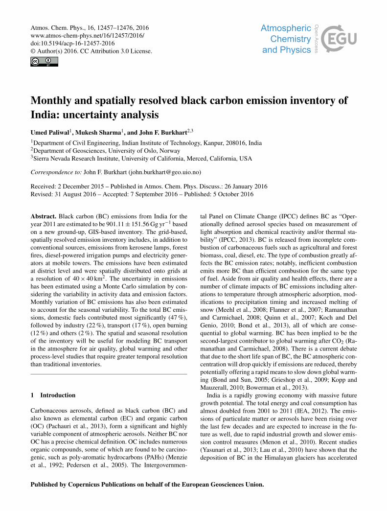
The spatial distribution of national emissions is presentedin Fig. 8. From the map it can be easily concluded that theIndo-Gangetic Plain (IGP) is the main contributor to nationalBC emissions. This can be attributed to the very high pop-ulation density and presence of major BC emitting indus-tries like sugar and brick production in this region. Some ofthe states in the IGP are among the least developed in In-dia, with little access to even basic amenities like electricity,clean cooking fuels, sanitation, health care, etc. More than90 % of the rural households in Uttar Pradesh and Bihar usebiomass fuels as their primary source of cooking, and morethan 65 % are dependent upon kerosene lamps as their pri-mary source of lighting (NSSO, 2015). The high dependenceon biomass fuels and the presence of brick and sugar indus-try accentuates the emissions from this region. With annualemissions of 140 Gg, the state of Uttar Pradesh emits themost in the IGP followed by West Bengal (57.67 Gg), Bi-har (47.8 Gg), Punjab (34.01 Gg), Haryana (26.82 Gg) andthe National Capital Territory (NCT) of Delhi (6.74 Gg). Themajor emissions sources in Uttar Pradesh are kerosene lamps(12 %), biomass cooking fuels (30 %), brick kilns (20 %) andsugar mills (17 %). High emissions from IGP and its vicinityto the Himalayas potentially pose a serious threat to water se-curity in the region, resulting from impacts on the cryospherefrom BC deposition and atmospheric heating.

www.atmos-chem-phys.net/16/12457/2016/ Atmos. Chem. Phys., 16, 12457–12476, 2016

12468 U. Paliwal et al.: India BC uncertainty

Figure 8. (a–d) Maps of major sector emissions and (e) spatial variability of national emissions total for BC.

Figure 9. Gen. extreme value distribution fit for the national BC emissions.

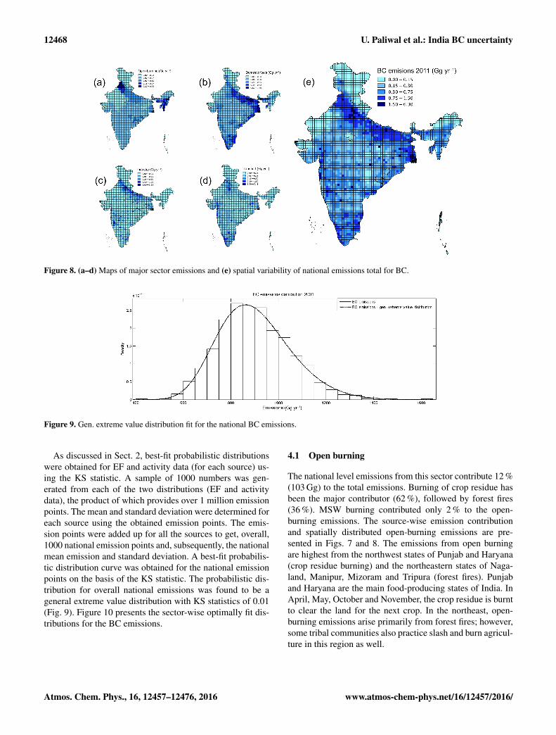
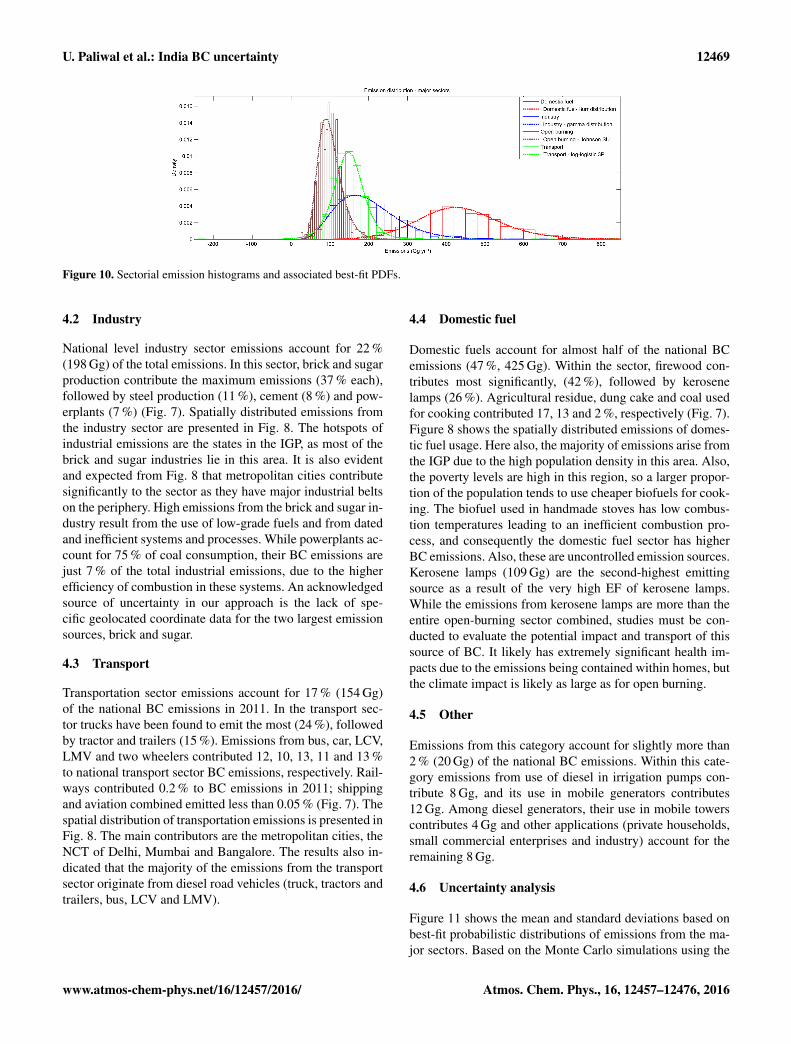
As discussed in Sect. 2, best-fit probabilistic distributionswere obtained for EF and activity data (for each source) us-ing the KS statistic. A sample of 1000 numbers was gen-erated from each of the two distributions (EF and activitydata), the product of which provides over 1 million emissionpoints. The mean and standard deviation were determined foreach source using the obtained emission points. The emis-sion points were added up for all the sources to get, overall,1000 national emission points and, subsequently, the nationalmean emission and standard deviation. A best-fit probabilis-tic distribution curve was obtained for the national emissionpoints on the basis of the KS statistic. The probabilistic dis-tribution for overall national emissions was found to be ageneral extreme value distribution with KS statistics of 0.01(Fig. 9). Figure 10 presents the sector-wise optimally fit dis-tributions for the BC emissions.

4.1 Open burning

The national level emissions from this sector contribute 12 %(103 Gg) to the total emissions. Burning of crop residue hasbeen the major contributor (62 %), followed by forest fires(36 %). MSW burning contributed only 2 % to the open-burning emissions. The source-wise emission contributionand spatially distributed open-burning emissions are pre-sented in Figs. 7 and 8. The emissions from open burningare highest from the northwest states of Punjab and Haryana(crop residue burning) and the northeastern states of Naga-land, Manipur, Mizoram and Tripura (forest fires). Punjaband Haryana are the main food-producing states of India. InApril, May, October and November, the crop residue is burntto clear the land for the next crop. In the northeast, open-burning emissions arise primarily from forest fires; however,some tribal communities also practice slash and burn agricul-ture in this region as well.

Atmos. Chem. Phys., 16, 12457–12476, 2016 www.atmos-chem-phys.net/16/12457/2016/

U. Paliwal et al.: India BC uncertainty 12469

Figure 10. Sectorial emission histograms and associated best-fit PDFs.

4.2 Industry

National level industry sector emissions account for 22 %(198 Gg) of the total emissions. In this sector, brick and sugarproduction contribute the maximum emissions (37 % each),followed by steel production (11 %), cement (8 %) and pow-erplants (7 %) (Fig. 7). Spatially distributed emissions fromthe industry sector are presented in Fig. 8. The hotspots ofindustrial emissions are the states in the IGP, as most of thebrick and sugar industries lie in this area. It is also evidentand expected from Fig. 8 that metropolitan cities contributesignificantly to the sector as they have major industrial beltson the periphery. High emissions from the brick and sugar in-dustry result from the use of low-grade fuels and from datedand inefficient systems and processes. While powerplants ac-count for 75 % of coal consumption, their BC emissions arejust 7 % of the total industrial emissions, due to the higherefficiency of combustion in these systems. An acknowledgedsource of uncertainty in our approach is the lack of spe-cific geolocated coordinate data for the two largest emissionsources, brick and sugar.

4.3 Transport

Transportation sector emissions account for 17 % (154 Gg)of the national BC emissions in 2011. In the transport sec-tor trucks have been found to emit the most (24 %), followedby tractor and trailers (15 %). Emissions from bus, car, LCV,LMV and two wheelers contributed 12, 10, 13, 11 and 13 %to national transport sector BC emissions, respectively. Rail-ways contributed 0.2 % to BC emissions in 2011; shippingand aviation combined emitted less than 0.05 % (Fig. 7). Thespatial distribution of transportation emissions is presented inFig. 8. The main contributors are the metropolitan cities, theNCT of Delhi, Mumbai and Bangalore. The results also in-dicated that the majority of the emissions from the transportsector originate from diesel road vehicles (truck, tractors andtrailers, bus, LCV and LMV).

4.4 Domestic fuel

Domestic fuels account for almost half of the national BCemissions (47 %, 425 Gg). Within the sector, firewood con-tributes most significantly, (42 %), followed by kerosenelamps (26 %). Agricultural residue, dung cake and coal usedfor cooking contributed 17, 13 and 2 %, respectively (Fig. 7).Figure 8 shows the spatially distributed emissions of domes-tic fuel usage. Here also, the majority of emissions arise fromthe IGP due to the high population density in this area. Also,the poverty levels are high in this region, so a larger propor-tion of the population tends to use cheaper biofuels for cook-ing. The biofuel used in handmade stoves has low combus-tion temperatures leading to an inefficient combustion pro-cess, and consequently the domestic fuel sector has higherBC emissions. Also, these are uncontrolled emission sources.Kerosene lamps (109 Gg) are the second-highest emittingsource as a result of the very high EF of kerosene lamps.While the emissions from kerosene lamps are more than theentire open-burning sector combined, studies must be con-ducted to evaluate the potential impact and transport of thissource of BC. It likely has extremely significant health im-pacts due to the emissions being contained within homes, butthe climate impact is likely as large as for open burning.

4.5 Other

Emissions from this category account for slightly more than2 % (20 Gg) of the national BC emissions. Within this cate-gory emissions from use of diesel in irrigation pumps con-tribute 8 Gg, and its use in mobile generators contributes12 Gg. Among diesel generators, their use in mobile towerscontributes 4 Gg and other applications (private households,small commercial enterprises and industry) account for theremaining 8 Gg.

4.6 Uncertainty analysis

Figure 11 shows the mean and standard deviations based onbest-fit probabilistic distributions of emissions from the ma-jor sectors. Based on the Monte Carlo simulations using the

www.atmos-chem-phys.net/16/12457/2016/ Atmos. Chem. Phys., 16, 12457–12476, 2016

12470 U. Paliwal et al.: India BC uncertainty

Figure 11. Mean and standard deviation for each of the major sec-tors of emissions for India, 2011.

multiple emissions estimates and available information onuncertainty, the PDFs for each of the sectors is calculatedas shown in Fig. 10. The best-fit distribution for the domes-tic fuels sector was found to be a Burr distribution with a KSstatistic of 0.01; for industrial emissions, it was a gamma dis-tribution with KS statistics of 0.02; for open-burning emis-sions, it was a Johnson SU distribution with a KS statisticof 0.02; and it was log-logistic (3P) for the transport sec-tor, with a KS statistic of 0.03. The uncertainty is highest foremissions from the domestic fuels sector. The EFs and ac-tivity data for the sources in the domestic fuel sector showa large variation leading to high uncertainty in the BC emis-sions as there is no accurate database of the population usingcookstoves, of the quantity of fuel consumed and the stoves’efficiency.

4.7 Comparison with prior estimates

Emissions in this study have been determined using a MonteCarlo simulation of multiple activity data and emission fac-tors. As previous studies have used point estimates for thesehighly uncertain quantities, the results are bound to differ.Figure 12 presents the comparison of the results of this study(Table 3) with emission inventories developed in the past.For the base year 2011, the estimate is about 80 % of thatreported in the SAFAR emission inventory (1119 Gg yr−1).For inventories with base year 2010, total national emis-sions estimated in this study are a factor of 1.3 higher thanRETRO (697 Gg yr−1), factor of 0.8 of that estimated inKlimont et al. (2009) (1104 Gg yr−1), a factor of 0.9 of thatestimated in Lu et al. (2011) (1015 Gg yr−1), and they werein agreement with emissions determined by Ohara et al.(2007) (862 Gg yr−1). All prior national emission estimateslie within 2 standard deviations of our mean estimate.

Emissions estimates from the domestic fuels sector(425± 112 Gg yr−1) are lower by a factor of 0.7–0.9 thanPandey et al. (2014) (488 Gg yr−1), Klimont et al. (2009)

Table 3. Mean national emissions and standard deviation.

Sector/subsector Emissions (Gg yr−1)

Open burning 102.84± 27.56

Crop residue burning 64.31± 17.19Forest fire 36.90± 12.85Garbage burning 1.63± 0.62

Industry 198.5± 83.391

Brick 74.11± 61.38Steel 21.09± 32.18Sugar 72.76± 25.05Cement 15.45± 22.26Power 15.09± 23.88

Transport 154.34± 56.14

Bus 17.64± 8.72Car 14.69± 10.54LMV 17.01± 25.03LCV 20.62± 10.51Truck 37.46± 20.49Taxi 2.13± 1.44Two wheeler 20.11± 39.50Tractor and trailer 22.79± 11.41Railway 1.60± 1.32Shipping 0.15± 0.07Aviation 0.14± 0.04

Domestic fuel 425.36± 111.97

Dung cake 54.79± 48.15Agriculture residue 74.38± 44.17Firewood 177.34± 83.88Coal 9.02± 14.622Kerosene cooking 0.83± 0.19352LPG 0.47± 0.39Kerosene lamps 108.53± 27.10

Others 20.08± 2.59

Irrigation pumps 7.55± 1.73Diesel generators (mobile towers) 4.14± 0.85Diesel generators (other) 8.39± 1.73

Total 901.11± 151.56

(628 Gg yr−1) and Lu et al. (2011) (579 Gg yr−1). For thetransport sector our emission estimate (154± 56 Gg yr−1)is almost identical to that presented in Sadavarte andVenkataraman (2014) (144 Gg yr−1) and a factor of 1.1–1.3 higher than the emissions determined by Lu et al.(2011) (111 Gg yr−1), Baidya and Borken-Kleefeld (2009)(123 Gg yr−1) and Klimont et al. (2009) (136 Gg yr−1). Inthe industry sector our emissions (198± 83 Gg) are 10–20 %lower in view of the inclusion of only higher emitting indus-tries in this study. The combined industrial emission estimateof Sadavarte and Venkataraman (2014) (formal industry) andPandey et al. (2014) (informal industry) (212 Gg yr−1) is in

Atmos. Chem. Phys., 16, 12457–12476, 2016 www.atmos-chem-phys.net/16/12457/2016/

U. Paliwal et al.: India BC uncertainty 12471

Figure 12. Comparison of current BC emissions estimate with pre-viously published results for India. A: Streets et al. (2003) (baseyear 2000); B: Reddy and Venkataraman (2002a, 2002b) (base year1997); C: Sahu et al. (2008) (base year 2011); D: Schultz et al.(2008) (base year 2010); E: Lu et al. (2011) (base year 2010); F:Klimont et al. (2009) (base year 2010); G: Ohara et al. (2007) (baseyear 2010); H: this study (base year 2011).

good agreement with our emission estimate (factor 0.94). Es-timated industrial emissions are a factor of 0.8–0.9 lowerthan Lu et al. (2011) (227 Gg yr−1) and Klimont et al. (2009)(261 Gg yr−1). Emissions from open crop residue burning(64± 17 Gg yr−1) are in close agreement (factor 0.8–1) withJain (2014) (68 Gg yr−1), Lu et al. (2011) (74 Gg yr−1) andPandey et al. (2014) (80 Gg yr−1). Forest fire emissions(37± 13 Gg) are almost identical to those determined inReddy and Venkataraman (2002a) (39 Gg yr−1). As with thenational emission estimate, for all sectors prior emission es-timates are within 1 or 2 standard deviations from our meanemission estimate.

4.8 Fuel balance

A fuel balance approach has been used to ensure that nomajor emission source has been overlooked in our study.Since biomass consumption data in India are highly uncer-tain, this approach was only employed for emissions arisingfrom combustion of fossil fuels. Emissions from combustionof diesel, gasoline, fuel oil, ATF, LDO and coal were esti-mated using emission factors from Streets et al. (2003) andBond et al. (2004). In 2011, emission from these fuels was es-timated to be 281 Gg (Table 4). This was very close to emis-sions estimated from our methodology (304 Gg), consideringthe emission sources which use these fuels as a combustionsource.

4.9 Seasonality of emissions

There is a strong seasonality associated with BC emissionsin India. Crop residue burning, forest fires, and the brick

Table 4. Fuel balance.

Sector/fuel Activity EF Emission(Mt) (g kg−1) (Gg)

Coal 535.881 0.3282 175.77Gasoline/petrol 14.4423 2.7954 40.37Diesel 63.5043 1.024 64.77Fuel oil 6.6243 0.044 0.26ATF 5.3243 0.034 0.16

Total 281.33

1MoSPI (2014a). 2Streets et al. (2003). 3MoPNG (2014). 4Bond et al.(2004).

and sugar industry have a seasonal dependence in emissions.Forest fires are predominant from February to July. MonthlyBC emissions from forest fires were estimated using MODISburnt-area data. The brick industry becomes active after themonsoon season from October to June (Maithel et al., 2012);the sugar industry operates from November to June (Tyagi,1995), and the emissions are equally distributed among themonths of operation. Burning of crop residues generally oc-curs in the harvesting months, which are October–Novemberfor kharif crop and April–May for rabi crop. Emissions ofagricultural open burning are equally distributed among themonths of April, May, October and November. For all theother sources, emission rates are assumed to be uniformthroughout the year. Using these data, monthly variation ofBC emissions has been estimated and is shown in Fig. 13.

The emissions in April are highest due to the burningof crop residues. Despite the absence of crop residue burn-ing, emissions in March are also high because of the emis-sions from forest fires. As we have shown that a considerableamount of the emissions comes from the IGP, which is inclose proximity to the Himalayas, this causes further concernregarding the potential cryospheric impact of these aerosolsas they are strongest during the period when the seasonalsnowmelt period is beginning and they could be incorporatedinto the snowpack.

5 Conclusions

A spatially resolved BC emission inventory for 2011 hasbeen developed, considering major sectors and with carefulconsideration of subsector sources. The sources were classi-fied into five major sectors: (i) open burning, including for-est fire emissions, open solid-waste burning and agricultureresidue burning; (ii) industry, including brick industry, ce-ment, steel plants, sugar mills and powerplants; (iii) trans-port, including two wheelers, cars, light motor vehicles pas-senger, light commercial vehicles, taxies, trucks, buses, trac-tors and trailers, railways, shipping, and airways; (iv) do-mestic fuel, including firewood burning, agricultural residue,coal, liquid petroleum gas, kerosene (cooking and lighting)

www.atmos-chem-phys.net/16/12457/2016/ Atmos. Chem. Phys., 16, 12457–12476, 2016

12472 U. Paliwal et al.: India BC uncertainty

Figure 13. Time series of monthly emissions for India, 2011. Notethe strong seasonality of the open-burning and industry sector. Inthe latter case, the seasonality results predominately from sugarcaneproduction.

and dung cake; and (v) “other”, including use of diesel in ir-rigation pumps and for other power generation in diesel gen-erators.

This is a first-of-its-kind comprehensive study which in-cluded sources such as kerosene lamps and forest fires thatwere not part of earlier emission inventories. Furthermore,for each sector, source uncertainties in emissions have beenestimated based on variability in available activity data andemission factors. Lastly, and significantly, we provide our es-timate of emissions at a monthly temporal resolution on aspatially distributed 40× 40 km. grid.

The national BC emissions for India in 2011 are estimatedto be 901± 152 Gg yr−1, with domestic fuels contributingthe most (47 %), followed by industries (22 %), transport(17 %), open burning (12 %) and others (2 %). Large emis-sion in the domestic fuels sector stems from the extensiveuse of biomass for cooking in India. Firewood is the sin-gle largest emitter, with 177 Gg (20 %) of BC emissions in2011. The emissions from firewood are more than the entiretransportation sector combined. Kerosene lamps surprisinglycontribute 12 % to the national BC emissions. The emissionshave been found to be have a significant seasonality, varyingfrom 55 Gg in July to 90 Gg in April 2011.

The results of the study could be used to assess the con-tribution of different sources to national and regional emis-sions. The spatial resolution of the inventory should be usefulfor modeling the black carbon processes in the atmospherethrough air quality models. Monthly gridded emission datasets can also be prepared for finer temporal-resolution input.To improve the future BC emission estimates, local emissionfactors and activity data should be improved, especially fordomestic fuels and the brick industry. The emission inven-tory can be improved nationally, regionally and temporally

by comparing the modeled emission estimates (providing theinventory as input to air quality models) with the observeddata.

6 Data availability

The inventory is available from the authors on request.More information may be found at http://www.mn.uio.no/geo/english/research/projects/hycamp.

Acknowledgement. This work was conducted within the Nor-wegian Research Council’s INDNOR: Hydrologic sensitivityto Cryosphere-Aerosol interaction in Mountain Processes (Hy-CAMP) (Researcher project – MILJØ2015 no. 222195) and TheDepartment of Science and Technology, Government of India,through Grant no. INT/NOR/RCN/P-05/2013. We are grateful forconstructive feedback received from two anonymous reviewers andour editor, who encouraged the addition of the road network andincorporating the fuel balance analysis.

Edited by: C. HooseReviewed by: three anonymous referees

References

Abhilash, P. C. and Singh, N.: Influence of the application of sugar-cane bagasse on lindane (γ -HCH) mobility through soil column:Implication for biotreatment, Bioresource Technol., 99, 8961–8966, doi:10.1016/j.biortech.2008.05.006, 2008.

Akagi, S. K., Yokelson, R. J., Wiedinmyer, C., Alvarado, M. J.,Reid, J. S., Karl, T., Crounse, J. D., and Wennberg, P. O.: Emis-sion factors for open and domestic biomass burning for usein atmospheric models, Atmos. Chem. Phys., 11, 4039–4072,doi:10.5194/acp-11-4039-2011, 2011.

Andreae, M. O. and Merlet, P.: Emission of trace gases and aerosolsfrom biomass burning, Global Biogeochem. Cy., 15, 955–966,doi:10.1029/2000GB001382, 2001.

ARAI: Air Quality Monitoring Project-Indian Clean Air Pro-gramme (ICAP), Draft report on Emission Factor developmentfor Indian Vehicles, Tech. rep., The Automotive Research Asso-ciation of India, 2008.

Baidya, S. and Borken-Kleefeld, J.: Atmospheric emissions fromroad transportation in India, Energy Policy, 37, 3812–3822,doi:10.1016/j.enpol.2009.07.010, 2009.

Bond, T. C. and Sun, K.: Can reducing black carbon emissionscounteract global warming?, Environ. Sci. Technol., 39, 5921–5926, doi:10.1021/es0480421, 2005.

Bond, T. C., David G., S., Kristen F., Y., Sibyl M., N., Jung-Hun,W., and Zbigniew, K.: A technology-based global inventory ofblack and organic carbon emissions from combustion, J. Geo-phys. Res., 109, D14203, doi:10.1029/2003JD003697, 2004.

Bond, T. C., Bhardwaj, E., Dong, R., Jogani, R., Jung, S., Ro-den, C., Streets, D. G., and Trautmann, N. M.: Historical emis-sions of black and organic carbon aerosol from energy-relatedcombustion, 1850–2000, Global Biogeochem. Cy., 21, GB2018,doi:10.1029/2006GB002840, 2007.

Atmos. Chem. Phys., 16, 12457–12476, 2016 www.atmos-chem-phys.net/16/12457/2016/

U. Paliwal et al.: India BC uncertainty 12473

Bond, T. C., Doherty, S. J., Fahey, D. W., Forster, P. M., Berntsen,T., Deangelo, B. J., Flanner, M. G., Ghan, S., Kärcher, B.,Koch, D., Kinne, S., Kondo, Y., Quinn, P. K., Sarofim, M. C.,Schultz, M. G., Schulz, M., Venkataraman, C., Zhang, H., Zhang,S., Bellouin, N., Guttikunda, S. K., Hopke, P. K., Jacobson,M. Z., Kaiser, J. W., Klimont, Z., Lohmann, U., Schwarz, J. P.,Shindell, D., Storelvmo, T., Warren, S. G., and Zender, C. S.:Bounding the role of black carbon in the climate system: A sci-entific assessment, J. Geophys. Res.-Atmos., 118, 5380–5552,doi:10.1002/jgrd.50171, 2013.

Borken, J., Steller, H., Merétei, T., and Vanhove, F.: Global andCountry Inventory of Road Passenger and Freight Transporta-tion: Fuel Consumption and Emissions of Air Pollutants inYear 2000, Transportation Research Record, 2011, 127–136,doi:10.3141/2011-14, 2008.

Bowerman, N. H. A., Frame, D. J., Huntingford, C., Lowe, J. A.,Smith, S. M., and Allen, M. R.: The role of short-lived climatepollutants in meeting temperature goals, Nature Climate Change,3, 1021–1024, doi:10.1038/nclimate2034, 2013.

Cachier, H.: Carbonaceous combustion aerosols, in: AtmosphericParticles, edited by: Harrison, R. and van Grieken, R., vol. 2, pp.1–2, pp. 295-348, John Wiley, New York, 1998.

CEA: Annual report on fuel consumption in Power Plants, Tech.rep., Central Electricity Authority, New Delhi, available at: http://www.cea.nic.in (last access: January 2015), 2012.

CEA-LGBR: Load generation balance report 2012-13, 2013-14,Tech. rep., Central Electricity Authority, Ministry of Power, Gov-ernment of India, New Delhi, 2013.

Census of India: India: Administrative Divisions 2011, avail-able at: http://www.censusindia.gov.in/2011census/maps/atlas/00part1.pdf (last access: April 2015), 2011.

Chen, Y., Sheng, G., Bi, X., Feng, Y., Mai, B., and Fu, J.: Emissionfactors for carbonaceous particles and polycyclic aromatic hy-drocarbons from residential coal combustion in China, Environ.Sci. Technol., 39, 1861–1867, doi:10.1021/es0493650, 2005.

Chen, Y., Zhi, G., Feng, Y., Liu, D., Zhang, G., Li, J., Sheng, G.,and Fu, J.: Measurements of black and organic carbon emis-sion factors for household coal combustion in China: Implicationfor emission reduction, Environ. Sci. Technol., 43, 9495–9500,doi:10.1021/es9021766, 2009.

Chow, J. C., Watson, J. G., Lowenthal, D. H., Antony Chen, L. W.,and Motallebi, N.: PM2.5 source profiles for black and organiccarbon emission inventories, Atmos. Environ., 45, 5407–5414,doi:10.1016/j.atmosenv.2011.07.011, 2011.

CMA: Annual Report 2011-12, Tech. rep., Cement Manufacturers’Association, New Delhi, available at: http://www.cmaindia.org/cms/images/annual-report/Annual-Report-2011-12.pdf, 2012.

Cooke, W. F., Liousse, C., Cachier, H., and Feichter, J.: Construc-tion of Construction of a 1◦ × 1◦ fossil fuel emission data setfor carbonaceous aerosol and implementation radiative impactin the ECHAM4 model, J. Geophys. Res., 104, 22137–22162,doi:10.1029/1999JD900187, 1999.

CPCB: Management of Municipal Solid Waste, Tech. rep., CentralPollution Control Board, Government of India, New Delhi, 2007.

CPCB: Status Report on Municipal Solid Waste Management, Tech.rep., Ministry of Environment & Forests, Government of India,New Delhi, 2012.

DAC: Annual Report 2012-13, Tech. rep., Department of Agricul-ture and Cooperation, Government of India, New Delhi, 2013.

DFPD: Department of Food and Public Distribution, available at:http://dfpd.nic.in/ (last access: January 2015), 2011.

DGCA: Air Transport Statistics 2011-12 & 2012-13, Tech. rep., Di-rectorate General of Civil Aviation, Government of India, NewDelhi, 2013.

EEA: The impact of international shipping on European air qual-ity and climate forcing, Tech. Rep. 4, European EnvironmentAgency, doi:10.2800/75763, 2013.

Ezhumalai, S. and Thangavelu, V.: Kinetic and optimization stud-ies on the bioconversion of lignocellulosic material into ethanol,BioResources, 5, 1879–1894, 2010.

Flanner, M. G., Zender, C. S., Randerson, J. T., and Rasch,P. J.: Present-day climate forcing and response from blackcarbon in snow, J. Geophys. Res.-Atmos., 112, D11202,doi:10.1029/2006JD008003, 2007.

FSI: State of Forest Report 2013, Tech. rep., Forest Survey of India,Ministry of Environment & Forests, Government of India, NewDelhi, 2013.

FSI: Forest Fire Search – Forest Survey of India, available at: http://fsi.nic.in/forest-fire.php (last access: January 2015), 2015.

Ganguly, D., Ginoux, P., Ramaswamy, V., Winker, D. M., Hol-ben, B. N., and Tripathi, S. N.: Retrieving the composition andconcentration of aerosols over the Indo-Gangetic basin usingCALIOP and AERONET data, Geophys. Res. Lett., 36, L13806doi:10.1029/2009GL038315, 2009.

Grieshop, A. P., Reynolds, C. C. O., Kandlikar, M., andDowlatabadi, H.: A black-carbon mitigation wedge, NatureGeosci., 2, 533–534, doi:10.1038/ngeo595, 2009.

Gupta, S. and Narayan, R.: Brick kiln industry in long-term impactsbiomass and diversity structure of plant communities, CurrentSci., 99, 72–79, 2010.

Guttikunda, S. K. and Calori, G.: A GIS based emissions in-ventory at 1 km × 1 km spatial resolution for air pollu-tion analysis in Delhi, India, Atmos. Environ., 67, 101–111,doi:10.1016/j.atmosenv.2012.10.040, 2013.

Habib, G., Venkataraman, C., Shrivastava, M., Banerjee, R., Stehr,J. W., and Dickerson, R. R.: New methodology for estimat-ing biofuel consumption for cooking: Atmospheric emissions ofblack carbon and sulfur dioxide from India, Global Biogeochem.Cy., 18, GB3007, doi:10.1029/2003GB002157, 2004.

Heierli, U. and Maithel, S.: Brick By Brick : The Herculean Task ofCleaning Up the Asian, Tech. Rep. FEBRUARY 2008, NaturalResources and Environment Division, Swiss Agency for Devel-opment and Cooperation, 2015.

Hendricks, J., Kärcher, B., Döpelheuer, A., Feichter, J., Lohmann,U., and Baumgardner, D.: Simulating the global atmosphericblack carbon cycle: a revisit to the contribution of aircraft emis-sions, Atmos. Chem. Phys., 4, 2521–2541, doi:10.5194/acp-4-2521-2004, 2004.

ICAO: Environmental Report 2010, Tech. rep., International CivilAviation Organization, 2010.

IEA: International Energy Agency Statistics, available at: http://www.iea.org/statistics/ (last access: January 2015), 2012.

IPCC 2006: 2006 IPCC Guidelines for National Greenhouse GasInventories, Prepared by the National Greenhouse Gas Invento-ries Programme, edited by: Eggleston, H. S., Buendia, L., Miwa,K., Ngara, T., and Tanabe, K., IGES, Japan, 2006.

IPCC, 2013: Annex III: Glossary, edited by: Planton, S., in: Cli-mate Change 2013: The Physical Science Basis. Contribution of

www.atmos-chem-phys.net/16/12457/2016/ Atmos. Chem. Phys., 16, 12457–12476, 2016

12474 U. Paliwal et al.: India BC uncertainty

Working Group I to the Fifth Assessment Report of the Intergov-ernmental Panel on Climate Change, edited by: Stocker, T. F.,Qin, D., Plattner, G.-K., Tignor, M., Allen, S. K., Boschung, J.,Nauels, A., Xia, Y., Bex, V., and Midgley, P. M., Cambridge Uni-versity Press, Cambridge, United Kingdom and New York, NY,USA, doi:10.1017/CBO9781107415324.031.

ISMA: List of sugar mills in India, Bangladesh, Pakistan, Nepal& Sri Lanka, Tech. rep., Indian Sugar Mills Association, NewDelhi, India, 2012.

Ito, A. and Penner, J. E.: Historical emissions of carbona-ceous aerosols from biomass and fossil fuel burning for theperiod 1870-2000, Global Biogeochem. Cy., 19, GB2028,doi:10.1029/2004GB002374, 2005.

Jain, N.: Emission of Air Pollutants from Crop Residue Burn-ing in India, Aerosol and Air Quality Research, 14, 422–430,doi:10.4209/aaqr.2013.01.0031, 2014.

Janssen, N. A., Gerlofs-Nijland, M. E., Lanki, T., Salonen,R. O., Cassee, F., Hoek, G., Fischer, P., Brunekreef, B.,and Krzyzanowski, M.: Health effects of black carbon,Tech. rep., World Health Organization, available at: http://www.euro.who.int/en/health-topics/environment-and-health/air-quality/publications/2012/health-effects-of-black-carbon(last access: April 2015), 2012.

Joshi, V.: Biomass burning in India, in: Global Biomass Burning:Atmospheric, Climatic, and Biospheric Implications, 185–193,The MIT Press, Cambridge, London, 1991.

Klimont, Z., Cofala, J., Xing, J., Wei, W., Zhang, C., Wang, S., Ke-jun, J., Bhandari, P., Mathur, R., Purohit, P., Rafaj, P., Amann,M., Chambers, A., and Hao, J.: Projections of SO2, NOx andcarbonaceous aerosols emissions in Asia, Tellus B, 61, 602–617,doi:10.1111/j.1600-0889.2009.00428.x, 2009.

Koch, D. and Del Genio, A. D.: Black carbon semi-direct effectson cloud cover: review and synthesis, Atmos. Chem. Phys., 10,7685–7696, doi:10.5194/acp-10-7685-2010, 2010.

Kopp, R. E. and Mauzerall, D. L.: Assessing the climatic benefitsof black carbon mitigation, P. Natl. Acad. Sci. USA, 107, 11703–11708, doi:10.1073/pnas.0909605107, 2010.

Kumar, S.: Effective Waste Management in India, Tech. rep., IN-TECH CROATIA, 2010.

Lack, D. A., Corbett, J. J., Onasch, T., Lerner, B., Massoli, P.,Quinn, P. K., Bates, T. S., Covert, D. S., Coffman, D., Sierau, B.,Herndon, S., Allan, J., Baynard, T., Lovejoy, E., Ravishankara,A. R., and Williams, E.: Particulate emissions from commercialshipping: Chemical, physical, and optical properties, J. Geophys.Res.-Atmos., 114, D00F04, doi:10.1029/2008JD011300, 2009.

Lam, N. L., Chen, Y., Weyant, C., Venkataraman, C., Sadavarte, P.,Johnson, M. a., Smith, K. R., Brem, B. T., Arineitwe, J., Ellis,J. E., and Bond, T. C.: Household light makes global heat: Highblack carbon emissions from kerosene wick lamps, Environ. Sci.Technol., 46, 13531–13538, doi:10.1021/es302697h, 2012.

Land Processes Distributed Active Archive Center (LP DAAC),2000: MODIS MCD45A1, NASA EOSDIS Land ProcessesDAAC, USGS Earth Resources Observation and Science(EROS) Center, Sioux Falls, South Dakota, available at: https://lpdaac.usgs.gov, last access: January 2015.

Lau, W. K. M., Kim, M.-K., Kim, K.-M., and Lee, W.-S.: Enhancedsurface warming and accelerated snowmelt in the Himalayas andTibetan Plateau induced by absorbing aerosols, Env. Res. Lett.,5, 025204, doi:10.1088/1748-9326/5/2/025204, 2010.

Li, X., Wang, S., Duan, L., Hao, J., and Nie, Y.: Car-bonaceous Aerosol Emissions from Household Biofuel Com-bustion in China, Environ. Sci. Technol., 43, 6076–6081,doi:10.1021/es803330j, 2009.

Liousse, C., Penner, J. E., Chuang, C., Walton, J. J., Eddle-man, H., and Cachier, H.: A global three-dimensional modelstudy of carbonaceous aerosols, J. Geophys. Res., 101, 19411,doi:10.1029/95JD03426, 1996.

Lu, Z., Zhang, Q., and Streets, D. G.: Sulfur dioxide and primarycarbonaceous aerosol emissions in China and India, 1996–2010,Atmos. Chem. Phys., 11, 9839–9864, doi:10.5194/acp-11-9839-2011, 2011.

Maithel, S., Uma, R., Bond, T., Baum, E., and Thao, V.: Brick KilnsPerformance Assessment A Roadmap for Cleaner Brick Produc-tion in India, Tech. Rep. April, Greentech Knowledge Solutions,New Delhi, India, 2012.

Mathwave Technologies: Fitting tool EasyFit software, Tech. rep.,available at: www.mathwave.com (last access: January 2015),2015.

Meehl, G. A., Arblaster, J. M., and Collins, W. D.: Effects of blackcarbon aerosols on the Indian monsoon, J. Climate, 21, 2869–2882, doi:10.1175/2007JCLI1777.1, 2008.

Menon, S., Koch, D., Beig, G., Sahu, S., Fasullo, J., and Orlikowski,D.: Black carbon aerosols and the third polar ice cap, Atmos.Chem. Phys., 10, 4559–4571, doi:10.5194/acp-10-4559-2010,2010.

Menzie, C. A., Potocki, B. B., and Santodonato, J.: Am-bient concentrations and exposure to carcinogenic PAHsin the environment, Environ. Sci. Technol., 26, 1278–1284doi:10.1021/es00031a002, 1992.

Ministry of Agriculture: Land Use Statistics Information Sys-tem, available at: http://eands.dacnet.nic.in/ (last access: January2015), 2011.

Ministry of Agriculture: Agricultural Statistics at a Glance 2013,Tech. rep., Directorate of Economics and Statistics, Governmentof India, New Delhi, 2013.

Ministry of Railways: INDIAN RAILWAYS Year Book 2010-11, Tech. rep., Government of India, New Delhi, availableat: http://www.indianrailways.gov.in/railwayboard/uploads/directorate/stat_econ/yearbook10-11/Year_book_10-11_eng.pdf(last access: July 2015), 2012a.

Ministry of Railways: INDIAN RAILWAYS ANNUAL REPORT& ACCOUNTS, Tech. rep., Government of India, New Delhi,2012b.

Ministry of Road Transport and Highways: Road Transport YearBook 2010-11, Tech. rep., Government of India, New Delhi,2011.

Ministry of Steel: Annual Report 2012-13, Tech. rep., Governmentof India, New Delhi, 2014.

Mittal, L. M. and Sharma, C.: Anthropogenic Emissions fromEnergy Activities in India: Generation and Source Characteri-zation (Part II: Emissions from Vehicular Transport in India),Tech. rep., available at: http://archive.osc.edu/research/archive/pcrm/emissions/India_Report_1Pagelayout.pdf (last access: July2015), 2003.

Moorthy, K. K., Beegum, S. N., Srivastava, N., Satheesh, S. K.,Chin, M., Blond, N., Babu, S. S., and Singh, S.: Performanceevaluation of chemistry transport models over India, Atmos. En-viron., 71, 210–225, doi:10.1016/j.atmosenv.2013.01.056, 2013.

Atmos. Chem. Phys., 16, 12457–12476, 2016 www.atmos-chem-phys.net/16/12457/2016/

U. Paliwal et al.: India BC uncertainty 12475

MoPNG: All India Study on Sectoral Demand of Diesel & Petrol,Tech. rep., Ministry of Petroleum and Natural Gas, Governmentof India, New Delhi, 2013.

MoPNG: Indian Petroleum and Natural Gas Statistics 2013-14,Tech. rep., Ministry of Petroleum & Natural Gas Economics andStatistics Division, Government of India, New Delhi, 2014.

MoSPI: Energy Statistics 2014, Tech. rep., Central Statistics Office,Government of India, New Delhi, available at: http://mospi.nic.in/mospi_new/upload/Energy_Statistics_2013.pdf (last access:July 2015), 2014a.

MoSPI: Household Consumption of Various Goods and Services inIndia, Tech. Rep. 558, MOSPI, Government of India, New Delhi,2014b.

Nair, V. S., Solmon, F., Giorgi, F., Mariotti, L., Babu, S. S., andMoorthy, K. K.: Simulation of South Asian aerosols for re-gional climate studies, J. Geophys. Res.-Atmos., 117, D04209,doi:10.1029/2011JD016711, 2012.

National Environmental Engineering Research Institute (NEERI):Air Quality Assessment, Emissions Inventory and Source Ap-portionment Studies: Mumbai, New Delhi, Tech. rep., CentralPollution Control Board (CPCB), 2010, 2010.

Ni, M., Huang, J., Lu, S., Li, X., Yan, J., and Cen, K.: A review onblack carbon emissions, worldwide and in China., Chemosphere,107, 83–93, doi:10.1016/j.chemosphere.2014.02.052, 2014.

Novakov, T.: Large historical changes of fossil-fuelblack carbon aerosols, Geophys. Res. Let., 30, 1324,doi:10.1029/2002GL016345, 2003.

NSSO: Energy Sources of Indian Households for Cooking andLighting, 2011-12, National Sample Survey Office,Ministry ofStatistics and Programme Implementation, Government of India,New Delhi, available at: http://mospi.nic.in/mospi_new/upload/nss_report_567.pdf (last access: May 2015), 2015.

Ohara, T., Akimoto, H., Kurokawa, J., Horii, N., Yamaji, K., Yan,X., and Hayasaka, T.: An Asian emission inventory of an-thropogenic emission sources for the period 1980–2020, At-mos. Chem. Phys., 7, 4419–4444, doi:10.5194/acp-7-4419-2007,2007.

OpenStreetMap: OpenStreetMap Foundation – Geofabrik DataDownloads, available at: http://download.geofabrik.de/asia/india.html (last access: April 2015), 2016.

Pachauri, T., Satsangi, A., Singla, V., Lakhani, A., and Maharaj Ku-mari, K.: Characteristics and sources of carbonaceous aerosols inPM2.5 during wintertime in Agra, India, Aerosol and Air QualityResearch, 13, 977–991, doi:10.4209/aaqr.2012.10.0263, 2013.

Pandey, A. and Venkataraman, C.: Estimating emissions fromthe Indian transport sector with on-road fleet composi-tion and traffic volume, Atmos. Environ., 98, 123–133,doi:10.1016/j.atmosenv.2014.08.039, 2014.

Pandey, A., Sadavarte, P., Rao, A. B., and Venkataraman,C.: Trends in multi-pollutant emissions from a technology-linked inventory for India: II. Residential, agricultural andinformal industry sectors, Atmos. Environ., 99, 341–352,doi:10.1016/j.atmosenv.2014.09.080, 2014.

Parashar, D. C., Gadi, R., Mandal, T. K., and Mitra, A. P.: Carbona-ceous aerosol emissions from India, Atmos. Environ., 39, 7861–7871, doi:10.1016/j.atmosenv.2005.08.034, 2005.

Parikh, S. and Radhakrishna, R.: India Development Report 2004–05, Tech. rep., Oxford University Press, New Delhi, India, 2005.

Pedersen, D. U., Durant, J. L., Taghizadeh, K., Hemond, H. F.,Lafleur, A. L., and Cass, G. R.: Human cell mutagens in res-pirable airborne particles from the northeastern United States.2. Quantification of mutagens and other organic compounds,Environ. Sci. Technol., 39, 9547–9560, doi:10.1021/es050886c,2005.

Pessoa Júnior, A., de Mancilha, I. M., and Sato, S.: Evaluation ofsugar cane hemicellulose hydrolyzate for cultivation of yeastsand filamentous fungi, J. Ind. Microbiol. Biot., 18, 360–363,doi:10.1038/sj.jim.2900403, 1997.

Press Information Bureau: Number of Steel Plants in India, Govern-ment of India, New Delhi, available at: http://pib.nic.in/newsite/erelease.aspx?relid=77494 (last access: September 2015), 2011.

Qin, Y. and Xie, S.: Estimation of county-level black carbon emis-sions and its spatial distribution in China in 2000, Atmos. Envi-ron., 45, 6995–7004, doi:10.1016/j.atmosenv.2011.09.017, 2011.

Quinn, P. K., Bates, T. S., Baum, E., Doubleday, N., Fiore, A. M.,Flanner, M., Fridlind, A., Garrett, T. J., Koch, D., Menon, S.,Shindell, D., Stohl, A., and Warren, S. G.: Short-lived pollu-tants in the Arctic: their climate impact and possible mitigationstrategies, Atmos. Chem. Phys., 8, 1723–1735, doi:10.5194/acp-8-1723-2008, 2008.

Rajarathnam, U., Athalye, V., Ragavan, S., Maithel, S., Lalchan-dani, D., Kumar, S., Baum, E., Weyant, C., and Bond, T.: As-sessment of air pollutant emissions from brick kilns, Atmos. En-viron., 98, 549–553, doi:10.1016/j.atmosenv.2014.08.075, 2014.

Ramachandra, T. V. and Shwetmala: Emissions from India’s trans-port sector: Statewise synthesis, Atmos. Environ., 43, 5510–5517, doi:10.1016/j.atmosenv.2009.07.015, 2009.

Ramachandra, T. V., Aithal, B., and Sreejith, K.: GHG footprintof major cities in India, Renew. Sustain. Energy, 44, 473–495,doi:10.1016/j.rser.2014.12.036, 2015.

Ramanathan, V. and Carmichael, G.: Global and regional climatechanges due to black carbon, 1, 221–227, doi:10.1038/ngeo156,2008.

Reddy, M. and Venkataraman, C.: Inventory of aerosol and sul-phur dioxide emissions from India. Part II – biomass combustion,doi:10.1016/S1352-2310(01)00464-2, 2002a.

Reddy, M. S. and Venkataraman, C.: Inventory of aerosol and sul-phur dioxide emissions from India: I F Fossil fuel combustion,36, 677–697, 2002b.

Reynolds, C. C. O. and Kandlikar, M.: Climate impacts of air qual-ity policy: Switching to a natural gas-fueled public transportationsystem in New Delhi, Environ. Sci. Technol., 42, 5860–5865,doi:10.1021/es702863p, 2008.

Sadavarte, P. and Venkataraman, C.: Trends in multi-pollutantemissions from a technology-linked inventory for India: I. In-dustry and transport sectors, Atmos. Environ., 99, 353–364,doi:10.1016/j.atmosenv.2014.09.081, 2014.

Sahu, S. K., Beig, G., and Sharma, C.: Decadal growth of blackcarbon emissions in India, Geophys. Res. Lett., 35, L02807,doi:10.1029/2007GL032333, 2008.

Saud, T., Gautam, R., Mandal, T. K., Gadi, R., Singh, D. P., Sharma,S. K., Dahiya, M., and Saxena, M.: Emission estimates of organicand elemental carbon from household biomass fuel used over theIndo-Gangetic Plain (IGP), India, Atmos. Environ., 61, 212–220,doi:10.1016/j.atmosenv.2012.07.030, 2012.

Schultz, M., Backman, L., Balkanski, Y., Bjoerndalsaeter, S.,Brand, R., Burrows, J., Dalsoeren, S., de Vasconcelos, M., Grodt-

www.atmos-chem-phys.net/16/12457/2016/ Atmos. Chem. Phys., 16, 12457–12476, 2016

12476 U. Paliwal et al.: India BC uncertainty

mann, B., Hauglustaine, D., Heil, A., Hoelzemann, J., Isaksen, I.,Kaurola, J., Knorr, W., Ladstaetter-Weißenmayer, A., Mota, B.,Oom, D., Pacyna, J., Panasiuk, D., Pereira, J., Pulles, T., Pyle, J.,Rast, S., Richter, A., Savage, N., Schnadt, C., Schulz, M., Spessa,A., Staehelin, J., Sundet, J., Szopa, S., Thonicke, K., van hetBolscher, M., van Noije, T., van Velthoven, P., Vik, A., and Wit-trock, F.: REanalysis of the TROpospheric chemical composi-tion over the past 40 years. A long-term global modeling studyof tropospheric chemistry funded under the 5th EU frameworkprogramme, Final Report, Tech. Rep. 3, Max Planck Institute forMeteorology, Hamburg, 2007.

Schultz, M., Rast, S., Pulles, T., Brand, R., Pereira, J., Mota, B., andSpessa, A.: Emission data sets and methodologies for estimatingemissions, Tech. Rep. February 2007, Max Planck Institute forMeteorology, Hamburg, Germany, 2008.

Sen, A., Mandal, T., Sharma, S., Saxena, M., Gupta, N., Gautam,R., Gupta, A., Gill, T., Rani, S., Saud, T., Singh, D., and Gadi,R.: Chemical properties of emission from biomass fuels used inthe rural sector of the western region of India, Atmos. Environ.,99, 411–424, doi:10.1016/j.atmosenv.2014.09.012, 2014.

Shakti Sustainable Energy Foundation: Diesel Generators:Improving Efficiency and Emission Performance in In-dia, Shakti Sustainable Energy Foundation, availableat: http://shaktifoundation.in/wp-content/uploads/2014/02/Shakti-Diesel-Generators-FINAL1.pdf (last access: May 2015),2014.

Shen, G., Yang, Y., Wang, W., Tao, S., Zhu, C., Min, Y., Xue, M.,Ding, J., Wang, B., Wang, R., Shen, H., Li, W., Wang, X., andRussell, A. G.: Emission factors of particulate matter and el-emental carbon for crop residues and coals burned in typicalhousehold stoves in China, Environ. Sci. Technol., 44, 7157–7162, doi:10.1021/es101313y, 2010.

Shen, G., Wei, S., Wei, W., Zhang, Y., Min, Y., Wang, B., Wang,R., Li, W., Shen, H., Huang, Y., Yang, Y., Wang, W., Wang,X., Wang, X., and Tao, S.: Emission factors, size distributions,and emission inventories of carbonaceous particulate matter fromresidential wood combustion in rural china, Environ. Sci. Tech-nol., 46, 4207–4214, doi:10.1021/es203957u, 2012.

Sindhwani, R. and Goyal, P.: Assessment of traffic-generatedgaseous and particulate matter emissions and trends over Delhi(2000–2010), Atmospheric Pollution Research, 5, 438–446,doi:10.5094/APR.2014.051, 2014.

Smith, K., Uma, R., Kishore, V., Lata, K., Joshi, V., Zhang, J.,Rasmussen, R., and Khalil, M.: Greenhouse Gases from Small-scale Combustion Devices in Developing Countries, Phase IIA:Household Stoves in India, Tech. Rep. June, US EnvironmentalProtection Agency, Office of Research and Development, Wash-ington, DC 20460, EPA-600/R-00-052, 2000.

Sonkar, M.: Regional Scale Transport Simulation and Deposition ofElemental Carbon in the Himalayas: A WRF and CAMx Model-ing, Ph.D. thesis, IIT Kanpur, 2011.

Streets, D. G., Gupta, S., Waldhoff, S. T., Wang, M. Q., Bond,T. C., and Yiyun, B.: Black carbon emissions in China, Atmos.Environ., 35, 4281–4296, doi:10.1016/S1352-2310(01)00179-0,2001.

Streets, D. G., Yarber, K., Woo, J., and Carmichael, G.: An inven-tory of gaseous and primary aerosol emissions in Asia in the year2000, J. Geophys. Res., 108, 8809, doi:10.1029/2002JD003093,2003.

TERI (The Energy and Resources Institute): A Model to Estab-lish a Policy Framework for Emissions Reduction, and cost-effectiveness of Alternative Measures, Tech. rep., TERI, NewDelhi, 2006.

Turn, S. Q., Jenkins, B. M., Chow, J. C., Pritchett, L. C., Campbell,D., Cahill, T., and Whalen, S. A.: Elemental characterization ofparticulate matter emitted from biomass burning: Wind tunnelderived source profiles for herbaceous and wood fuels, J. Geo-phys. Res.-Atmos., 102, 3683–3699, doi:10.1029/96JD02979,1997.

Tyagi, R. C.: Problems and Prospects of Sugar Industry in India,Mittal Publications (India), 1995.

Venkataraman, C., Habib, G., Eiguren-Fernandez, A., Miguel,A. H., and Friedlander, S. K.: Residential biofuels inSouth Asia: carbonaceous aerosol emissions and climateimpacts., Science (New York, N.Y.), 307, 1454–1456,doi:10.1126/science.1104359, 2005.

Venkataraman, C., Habib, G., Kadamba, D., Shrivastava, M., Leon,J.-F., Crouzille, B., Boucher, O., and Streets, D. G.: Emissionsfrom open biomass burning in India: Integrating the inventory ap-proach with high-resolution Moderate Resolution Imaging Spec-troradiometer (MODIS) active-fire and land cover data, GlobalBiogeochem. Cy., 20, GB2013, doi:10.1029/2005GB002547,2006.

Weyant, C., Athalye, V., Ragavan, S., Rajarathnam, U., Lalchan-dani, D., Maithel, S., Baum, E., and Bond, T. C.: Emissions fromSouth Asian brick production, Environ. Sci. Technol., 48, 6477–6483, doi:10.1021/es500186g, 2014.

World Bank: Access to electricity (% of population), available at:http://data.worldbank.org/indicator/EG.ELC.ACCS.ZS (last ac-cess: July 2016), 2010.

Yasunari, T. J., Tan, Q., Lau, K. M., Bonasoni, P., Marinoni,A., Laj, P., Ménégoz, M., Takemura, T., and Chin, M.: Es-timated range of black carbon dry deposition and the re-lated snow albedo reduction over Himalayan glaciers dur-ing dry pre-monsoon periods, Atmos. Environ., 78, 259–267,doi:10.1016/j.atmosenv.2012.03.031, 2013.

Yevich, R.: An assessment of biofuel use and burning of agricul-tural waste in the developing world, Global Biogeochem. Cy.,17, 1095, doi:10.1029/2002GB001952, 2003.

Zhang, Y., Shao, M., Lin, Y., Luan, S., Mao, N., Chen, W., andWang, M.: Emission inventory of carbonaceous pollutants frombiomass burning in the Pearl River Delta Region, China, Atmos.Environ., 76, 189–199, doi:10.1016/j.atmosenv.2012.05.055,2013.

Atmos. Chem. Phys., 16, 12457–12476, 2016 www.atmos-chem-phys.net/16/12457/2016/