moody's riskcalc™ for private companies: korea · for estimating firm default probabilities...

Rating Methodology

Contact PhoneNew YorkAhmet E. Kocagil 1.212.553.1653David BrenSeoulJean Rhee 82.2.3771.4728San FranciscoJeff Bohn 1.415.274.1700TokyoShota Ishii 81.3.5408.4000

AuthorsAhmet E. KocagilAlexander Reyngold

May 2003

Moody's RiskCalc™ For Private Companies: Korea
OverviewIn a continuing effort to provide benchmarks for private middle market companies, Moody’s KMV has built a modelfor estimating firm default probabilities for private Korean companies which utilizes local company financial state-ments. This model joins a network of international models covering private firms of the United States of America,Canada, Mexico, Germany, Spain, France, the United Kingdom, Belgium, the Netherlands, Portugal, Italy, Austria,Japan, Australia, Singapore, and the Nordic Region, as well a sectoral model for US privately-held banks.1 The Risk-Calc network allows one to consistently attach probabilities of default to firms throughout the world. As a powerfulobjective model based on data provided by our local Credit Research Database (CRD) initiative, RiskCalc Koreaserves the interests of institutions, borrowers and investors alike.
The following is a self-contained description of the development and validation of the Moody’s RiskCalc™ model forKorean private companies. However, some details are omitted as a more detailed handling of some of the methodology iscontained in RiskCalc™ for Private Companies: Moody’s Default Model and RiskCalc™ for Private Companies II: MoreResults and the Australian Model documents.

We have organized the remainder of this report as follows:1. Introduction2. Model Factors3. Modeling Framework4. Validation and Empirical Tests5. The Dataset6. Implementation Tips7. Conclusions8. Appendices9. References

1. For the most up to date list of available models, the reader is referred to Moody’s KMV website at http://www.moodyskmv.com.

Highlights1. We describe Moody’s RiskCalc™ for Korean companies, a predictive statistical model of default, the factors

in the model, the modeling approach, and the accuracy of the model.2. We find that in testing, RiskCalc Korea:

– outperforms publicly available alternatives by a significant margin in both in- and out-of-sample testing, and– uniformly has more power across – industry sectors, – firm sizes, and – historical time periods.

3. Moody’s RiskCalc for Korean companies was developed using Moody’s Credit Research Database, whichcontains over 115,000 financial statements from over 32,000 Korean middle market borrowers observedbetween 1986 and 2001. This dataset includes about 3,300 defaulted Korean private firms.

IntroductionExperience has shown that a key determinant of lending performance is the ability of institutions to correctly assess thecredit risk within their portfolios. Objective quantitative default models are becoming increasingly vital in this effort.

A selected list of the applications of default models includes: • Regulatory/Capital allocation: in their efforts to ensure the soundness of the financial system and to

encourage appropriate behavior, regulators are increasingly looking for objective, hard-to-manipulatemeasures of risk to use in capital allocation.

• Monitoring and Credit process optimization: while a single number may prove inferior to thejudgement of a credit expert, the default model can help to pinpoint those cases where humanjudgement adds the most value.

• Decisioning and Pricing: without an accurate measure of the risks involved in lending to middlemarket companies, shareholder value might be destroyed through sub-optimal pricing.

• Securitization: banks are increasingly seeking to offer their clients a full range of lending services, withoutdesiring to hold the full capital that this would require. At the same time, investors are seeking new classesassets, prompting a need for a transparent, objective measure for evaluating bank loans and otherobligations. Tools such as RiskCalc provide such measures and can facilitate the evaluation of non-Agencyrated credits within Colleteralized Debt Obligations (CDOs).2 As a consequence Moody's Investors Serviceis currently a major user of RiskCalc in the evaluation of non-Agency rated credits within CDOs.

These applications require a powerful, efficient tool that allows unambiguous comparison of the credit quality ofdifferent loans and companies. Furthermore, the accurate pricing and trading of credit risk also demands that any suchtool is calibrated to a probability of default. RiskCalc is designed to provide such an independent benchmark, tieddirectly to a probabilistic interpretation, for most credit decision needs.

We believe that in order for any tool to qualify as a benchmark it must satisfy the following conditions:

1. It must be understandableCustomers consistently indicate that it is as important for them to understand why a model works as it is for the modelto provide marginal improvements in accuracy. The ratios driving a particular assessment should be clear and intuitive.

2. PowerfulA model, which is unable to differentiate between good and bad companies, is clearly of little use in credit decisions. Aconsequence of a powerful tool is the willingness of experienced personnel to use it in pricing and decision making.

3. Calibrated to probabilities of default (PDs)While an uncalibrated model can be used to decline or accept credits, it is of little use in ensuring that anyrisk assumed is accurately priced and capitalized. Furthermore, it will be of little use for trading debt. Thus,a benchmark must be tied directly to probability measures through empirical calibration.

4. Empirically validatedWithout documented performance on large datasets, prudence dictates that a third-party model must be viewedskeptically. Such testing also gives the user confidence that the model is stable and has not been “overfitted”3.

If a model does not satisfy these criteria then, while it may be a useful tool, it cannot be considered a benchmarkfor the market. For example, market participants could not use a more powerful tool in secondary market transactionsif the model outputs had not been calibrated. While we are confident that the model we have developed for Koreanprivate companies is very powerful, we concede that theoretically more powerful models could exist that are tailoredfor some specialized portfolios. Nevertheless, the products that form the RiskCalc network are capable of being truebenchmarks: they are easy to use, intuitive, powerful, calibrated, and validated.

There are three steps that form the core of the RiskCalc modeling process: transformation, modeling, and map-ping. In the transformation stage variables are converted statistically from typically noisy raw data into more usefuland powerful representations that aid in default prediction. In the second step, these transformed variables are com-bined statistically to yield a risk score. In the third step, the score is mapped to an empirical default probability. Priorto these steps, significant analysis takes place to select a subset of variables that predict default well, and after the modelis built significant work is done to validate the model and give confidence that it is robust and will perform well in thefuture. Further details of our methodology can be found in the Modeling Framework section.

2. CDOs include CBOs and CLOs.3. Of course, the level of validation that can be performed depends on the amount of data that is available.

2 Moody’s Rating Methodology

Model FactorsMoody’s RiskCalc™ for Korean private companies uses five broad categories of risk: cash flow/profitability, capitalstructure, liquidity, activity, and size. This section provides a description of these ratios and explains how they are cal-culated, and how they are related to default behavior. As we discuss below, these relationships are an important compo-nent of the variable selection process.

In this section, we present the results of the transformation stage of our analysis graphically. In the x-axes of Fig-ures 1 through 7, the population is sorted by percentiles (according to the variable), and then the correspondingobserved default rates (for each bucket) are measured and reported on the y-axes. In Figures 1-7, a steeper slope indi-cates a higher discriminatory power of a given variable, whereas a continuous (upward or downward) slope throughoutsuggests that the power of the variable is not restricted to a subsegment of the population only. In interpreting thegraphs it is useful to recall that, by definition, the ranges of the underlying financial ratio that correspond to eachbucket vary from one variable to another.

Cash Flow: ProfitabilityClearly, one of the most intuitive risk factors when modeling default behavior is the cash flow, e.g. profitability anddebt coverage of the firm. One expects that higher profitability ratios should be positive signals for a firm and thus cor-respond to lower default probabilities.

In developing RiskCalc™ Korea, we evaluated a number of alternative measures of profitability and examinedtheir distinguishing power of the good companies from the risky ones as described above. Following our analysis, wefound that gross profit over current assets was a powerful ratio in predicting default behavior. We note that net incomeover total assets perform also reasonably well. Nevertheless, we chose the first ratio because it performs better: as it canbe seen in Figure 1 it is an overall steeper curve.

Our hypothesis that firms with lower profitability would subsequently default more frequently was confirmed bythe data, and can be seen in Figure 1 for both measures of profitability.

Figure 1: More Profitable Firms Are Less Likely To Default

0 0.5 1

Ratio Percentile

Defa

ult L

ikel

ihoo

d

Gross Profit to Current Assets Net Income to Total Assets

Moody’s Rating Methodology 3

Cash Flow: Debt CoverageThe ability of a given firm to fulfill its borrowing obligations based on its cash flow/income (debt coverage) is one ofthe key parameters of default prediction. Similar to the discussion above, we also evaluated a number of alternativedebt coverage ratios. We find that Earnings (EBITDA) expressed as a fraction of interest expense gives a fairly accurateindication of how well a firm will be able to service its debt in the event of a downturn.

Capital Structure: LeverageThe credit literature depicts leverage as an important measure of the credit risk of a firm since it measures the firm’sability to withstand unforeseen circumstances. Following the transformation analysis, we decided to capture the lever-age effect of a firm by its liabilities to assets (TL/TA) ratio in RiskCalc Korea model.

This ratio is an important indicator of a company’s financial stability because the more of the liabilities that cannotbe covered by liquid assets (expressed as a percentage of total assets) the worse the company will fare in a downturn.

The univariate default relationship is presented in Figure 3. As seen in the figure, TL/TA has a steeper slope thantotal liabilities minus retained earnings over fixed assets, and thus is a better predictor of default behavior.

Figure 2: Firms With More Debt Coverage Are Less Likely To Default

Figure 3: Higher Leveraged Firms Default More Frequently

0 0.5 1

Ratio Percentile

Defa

ult L

ikel

ihoo

d

EBITDA to Interest Expense Net Worth to Total Interest Expense

0 0.5 1Ratio Percentile

Defa

ult L

ikel

ihoo

d

Total Liabilities to Total Assets Total Liablities less Retained Earnings to Fixed Assets


Capital Structure: Retained EarningsRetained earnings expressed as a fraction of liabilities (or assets) can be thought in a similar vein, as a capital structuremeasure signaling about the cushion the company will have in downturn.

LiquidityThere are many different liquidity ratios in common usage, but at heart they measure similar things, differing gener-ally in how much value they place on different types of current assets. The RiskCalc™ Korea model uses cash andmarketable securities expressed as a portion of current assets. Figure 5 demonstrates that companies with lower cur-rent ratios and smaller holdings of cash and marketable securities tend to have higher default probabilities.

Figure 4: Firms With More Retained Earnings Are Less Likely To Default

Figure 5: Firms With Poor Liquidity Default More Frequently


Defa

ult L

ikel

ihoo

d

Retained Earnings to Total Assets Retained Earnings to Current Assets Retained Earnings to Total Liabilities


Defa

ult L

ikel

ihoo

d

Cash and M arketable Securities to Current Assets Current Assets less Inventories to Current Liabilities


ActivityWe examine the activity of firms by looking at their inventories to sales ratio. We expect that for a given level of inven-tories, higher sales would indicate a lower level of riskiness for the firm. Thus, one would predict that the default prob-ability would decline, as the magnitude of this ratio becomes smaller. Figure 6 illustrates that our expectation isverified by empirical data and that current liabilities to sales is less powerful than inventories to sales ratio.

SizeSize, by its nature, is a variable that is correlated with many financial statement inputs and the quality of financial state-ments. In empirical literature there are numerous studies testing the impact of size on various performance measuresof a given company. It should be noted that correlation of size with other variables is not of concern in RiskCalc Korea(see: Multicollinearity Check section in Validation and Empirical Tests). One typically proxies firm size by value of itsvarious assets, such as fixed or total assets. Figure 7 exhibits two alternative size measures - total and fixed assets in realvalues, i.e. adjusted for inflation, and their relationship to default behavior in Korea. Note that total assets variableexhibits stronger overall differentiating power in terms of a firm’s default likelihood.

It may be interesting to view the transformation functions that the model utilizes all at once. Figure 8 summarizesthese functions graphically by risk factors. One notes that the “good” ratios (such as profitability, coverage ratios, size,etc.) exhibit a negative slope so that a higher ratio value is associated with a reduced probability of default. In contrast,‘bad’ ratios (such as leverage ratios, Inventories/Sales ratio etc) tend to exhibit a positive slope so that a higher ratiovalue is associated with a higher probability of default.

Figure 6: Firms With Poor Inventories/Sales Ratios Default More Frequently

Figure 7: Firm Size Is Inversely Related To Default Probability

Ratio Percentile

Defa

ult L

ikel

ihoo

d

Inventory to Net Sales Current Liabilities to Net Sales

Ratio Percentile

Defa

ult L

ikel

ihoo

d

Total Assets Fixed Assets


Figure 8: RiskCalc Korea Model Variables

Gross Profit to Current Assets

Ratio Percentile

Defa

ult L

ikel

ihoo

dEBITDA to Interest Expense

Ratio Percentile

Defa

ult L

ikel

ihoo

d

Total Liabilities to Total Assets

Ratio Percentile

Defa

ult L

ikel

ihoo

d

Retained Earnings to Total Assets

Ratio Percentile

Defa

ult L

ikel

ihoo

d

Retained Earnings to Total Assets

Ratio Percentile

Defa

ult L

ikel

ihoo

d

Inventory to Net Sales

Ratio Percentile

Defa

ult L

ikel

ihoo

d

Real Assets

Ratio Percentile

Defa

ult L

ikel

ihoo

d


Modeling FrameworkRiskCalc™ for Korean private companies is a non-structural, empirical model that is estimated utilizing country-spe-cific empirical default and financial statement data. Our modeling approach values parsimony in both functional formand the number of inputs4. Our modeling approach can be briefly summarized in the following three steps: transfor-mation, modeling, and mapping.

• Univariate Analysis and Transformation: the aim of single factor analysis is to study individual relationshipsto default of a set of potentially relevant factors that could be regarded a priori as independent variables in thefinal model. In this step we also mini-model the factors and transform them.

• Model Specification and Estimation: once the individual factors have been analyzed, the next step is to specifya model, using a subset of the most powerful factors. These factors are combined in a logistic model and theirweights are optimized.

• Calibration: finally, once the model has been specified and its weights estimated it is necessary to map theoutput of the model, a score, to a specific probability of default.In this section, we discuss these steps in detail and then describe the characteristics of the final model that they

produce.

Univariate Analysis And TransformationA specific characteristic of credit scoring models based on financial statement information is the large number of vari-ables that could potentially be used to predict default. It is very easy to define hundreds of financial ratios, combiningall of the information contained in the financial statements of a company in different ways to assess its credit worthi-ness. However, this would likely lead to a model that would be overfitted. In other words, such a model would performwell on the development dataset but it would perform poorly outside of it, thus inhibiting its potential applicability forcredit analysis in the real world.

The way financial statement information is used to build the model is crucial in determining the capability androbustness of the final model in predicting default. In particular, some of the financial ratios that can be derived will beuseful to predict default, but others are likely to be spuriously related to the default variable. Furthermore, some of theratios can take extremely high or low values for some companies, without adding any information for default predic-tion purposes. These two facts highlight the importance of the variable selection and transformation processes that areperformed during the univariate factor analysis phase.

Given the large number of possible ratios, it is important to reduce the list of ratios that enter the final modelselection process. This screening of ratios is based on the following criteria:

• They must be intuitive. If the final model is to be intuitive and make business sense, it must includefactors that are intuitive and make business sense.

• They must be powerful. We want to keep in our set of potential regressors those factors that have a highdiscriminatory power between defaulted and non-defaulted companies.

• There must be enough observations. Developing and validating a model requires a large number ofobservations. Furthermore, a large number of missing values typically indicates that the information isdifficult to obtain, and hence it would not be prudent to include it in the final model.

We test the predictive power of each ratio using the accuracy ratio (AR) which measures the ability of a metric todifferentiate between firms that later went on to default from those that did not. Where a ratio demonstrates extremelysmall or no predictive power we exclude it from further analysis.

Having excluded counterintuitive or uninformative ratios in the previous steps, we transform the data by minimo-deling the selected factors to capture their relationship to default. As shown in Figure 95, this relationship is generallymonotonic, meaning that the slope is either always positive, so that a higher ratio value indicates a higher probabilityof default, or always negative, so that a lower ratio value indicates a higher probability of default6. It is also apparentfrom Figure 9 that in this example, the relationship is a non-linear one, which is typically the case.

4. A model that is complicated may not be very useful for the practitioners, as they would like to understand the drivers and the intuition of the model.5. The x-axis shows the percentile in which a particular ratio value lies, and the y-axis shows the default frequency that is observed for firms with ratios in that percentile. 6. Growth ratios typically exhibit a U-shaped relationship with default and thus are non-monotonic, per se.


Given this monotonicity we model the relationship to default so that we capture it in a smooth manner and “cap”extreme values as part of our transformation process. This “capping” not only eliminates the impact of outliers in theestimation of the parameters of the final model, but also ensures that the final score calculated for a firm is not dis-torted by the impact of a small number of observations in the “tails” of our data set. Moreover, it also reflects the factthat beyond a certain level, most ratios provide little additional information about default.

Model Specification And EstimationIn the second step, the selected transformed factors undergo a process of multivariate analysis, to determine the predictivepower of different combinations of these ratios. Starting with a list of 20 ratios there would be over 1 million possiblemodels that could be created, so it is important to follow some basic guidelines and limit the number possible models.

There is no set rule in determining how many ratios a particular rating model should contain: a model with too fewvariables will not capture all the relevant information, whereas another one with too many variables will be powerful in-sample, but unstable when applied elsewhere and will most likely have onerous data input requirements7. When decidingon the final model to use, we combined an analysis of the power of the different models, as measured by the accuracyratios, with our experience. Some of the considerations that went into the selection of the final ratios and model are:

• Data requirements for the user should be as low as possible.• The number of factors should not exceed the typical risk factors we have found to matter in default modeling.• The factors and their weights should be intuitive.• The model should have high explanatory power.• The model should not exhibit any detectable econometric problems, such as multicollinearity.

The modeling step involves using the transformed inputs within a multivariate model so that the weights assignedto the multivariate model are appropriately adjusted not only for their univariate power, but also for their power in thepresence of other, often correlated information. Thus the model accounts for correlations, just not through any directinteraction terms such as net income × sales growth.8

We then use these transformations as the input to a binary model that predicts default. In our case we estimate aprobit model, which uses the normal or Gaussian cumulative distribution function, specifically:

The advantage of the probit model, as opposed to, say, ordinary least squares, is that it specifically accounts for thefact that the output, being binary, is restricted to be between 0 and 1.

Figure 9: The Relation Between A Financial Statement Ratio And Default Is Generally Monotonic And Non-Linear

Transformations Illustrate How Ratios Affect The Model And Capture Nonlinear Relationships

7. Furthermore, from a statistical point-of-view, a large number of ratios increases the error/variance in the estimates of the weights for each factor. As the size of a devel-opment data set decreases the confidence one has about the significance risk of factors selected by a statistical procedure also decreases.

8. We are not categorically against such extensions, but we are very wary of the degrees of freedom they bring forth. Moreover, there are no obvious interactions within the data, and the number and type of non-obvious interactions is sufficiently numerous to introduce more error from overfitting than nuanced enhancement at this point.

Net Income/Assets: X

Prob

abilit

y of

Def

ault:

T(x

)

y = Prob (default | x; β, σ)=F(β'T(x)) = exp dtβ'T(x)/σ 1

2πt2

2(- )∞


The resulting model, once estimated, is a generalized linear model, in that it is a nonlinear9 function of a linearmodel: y=Φ(f(x,b)), where the linear part is simply

and the T(X)'s are the transformations (as in Figure 9, above).

Calibration MappingThe final part of the modeling consists of mapping the output of the model to probabilities of default.

As Figure 10 shows, the output of the model is mapped to empirical default probabilities: note that the ordinalranking along the x-axis implies that the output of the model could be in arbitrary units. We estimate the relationshipbetween model output and sample default probability using a smoothing algorithm.10

Finally, we adjust the mean sample default probability to our projected population default probability by simply mul-tiplying by a constant so that, over the entire sample, our average firm had 1 and 5 year default probabilities of 2.1%and 8.4%, respectively.11

In other words, the adjustment can be presented as:

To summarize, the transformation of input ratios constitute a transparent way of capturing the information thateach ratio carries about the likelihood of default. The probit model is an efficient method of determining the optimalweights for combining the input ratios coupled with expert review of the raw statistical output. Finally, the mappingtransforms the score output into easily interpretable probabilities of default, which in turn are mapped to a “.pd” ratinggrade scale12.

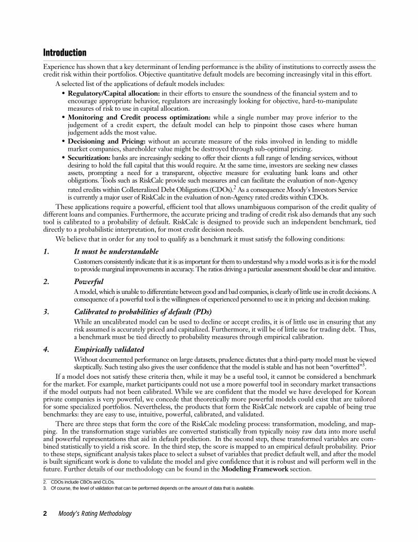
The RiskCalc Korea WeightsOne way to understand how the model works is to consider the approximate weightings13 on various factors. If weconsider broad risk categories we get the following weight distribution for the RiskCalc model for Korean privatecompanies. Top three risk factors are debt coverage, leverage and retained earnings, which are closely followed byprofitability, size and activity factors. Finally, liquidity accounts for about 8% of the overall weight in the model.

9. Specifically, a probit function.10. We use local regression techniques (loess) in this process.

Figure 10: Mapping To Sample Default Probabilities

Model Output Is Calibrated To Sample Default Probabilities Via A Smoothing Algorithm

11. See the discussion on the population default rate in the Dataset section.12. See Appendix C for a description of the relationship between the “.pd” rating grade scale used with RiskCalc models and the widely recognized Moody’s Investors Ser-

vice ratings grade scale.13. The reported figures are weights that correspond to the average firm in the sample.

f (x, β) = β0 + T1 (x1) β1 + T2 (x2) β2 + ... + T10 (x10) β10

0%2%4%6%8%

10%12%14%16%

1 2 3 4 5 6 7 8 9 10 11 12 13 14 15 16 17 18 19 20 21 22 23 24 25Immediate Model Output Bin

Defa

ult R

ate

Sample Bin Deafault Rate M apped Sample Default Rate

PDPopulation = PDSample xsample default rate

population default rate


To control for variations in the default rate across industry groups we adjust the constant term in the regression forthe industry. This calls for a positive adjustment in some industries, and negative in others. Figure 11 summarizes theimpacts of different industries on the estimated PD. Consistent with our previous modeling experience in severalother countries, the largest positive adjustment to the PD is observed in the case of construction industry. In the caseof mining industry, on the other hand the model reduces the estimated PD level.

Validation And Empirical TestsThe primary goals of validation and testing are to:

• determine how well a model performs;• ensure that a model has not been overfitted and that its performance is reliable and well understood;• confirm that the modeling approach, not just an individual model, is robust through time and credit cycles.

Model validation is an essential step to credit model development. We take care to perform tests in a rigorous androbust manner while also guarding against unintended errors. For example, it is important to compare all models onthe same data. We have found that the same model may get different performance results on different datasets, evenwhen there is no specific selection bias in choosing the data. To facilitate comparison, and avoid misleading results, weuse the same dataset to evaluate RiskCalc and competing models.

Model PowerHistorically, the primary model performance (power) measure employed by academic researchers has been the level ofmisclassification errors for a model, which assumes that there is some score/cut-off below which firms are rejected (andabove which they are accepted), and then measures the percentage of misclassifications.14 This measure is calculatedbased on the percentage of defaulting firms that are accepted, and the percentage of non-defaulting firms that arerejected, and depends upon the cut-off selected. Essentially, power curves extend this analysis by plotting the cumula-tive percentage of defaults excluded at each possible cut-off point for a given model.15

Table 1: Relative Weights Of Risk FactorsRiskCalc Korea

Debt coverage 24%Leverage 16%Retained Earnings 14%Profitability 11%Size 10%Activity 7%Liquidity 8%

Top Three Risk Factors Are Debt Coverage, Leverage And Retained Earnings

Figure 11: Relative Impact Of Industry

14. Statistically speaking, the Type I and Type II error rates, where Type I error indicates accepting a firm which defaults, and Type II indicates rejecting a firm which does not default.

15. In fact, if you know the default rate in a sample, you can calculate the Type I and Type II error rates for a particular cut-off from the power curve.

Manufacturing Construction Trade Services Mining,Transportation, and

UtilitiesIndustry Group

1 year 5year


One way of interpreting the power curve is that it illustrates the percentage of defaulting firms that would beexcluded as one excluded more and more of the worst “rated” firms in a data set. Thus one could interpret a powercurve, which went through (10%, 50%) as meaning that if one excluded the 10% of firms with the worst scores, onewould exclude 50% of all firms, which subsequently defaulted. In comparing the performance of two models on thesame data set,16 the more powerful model will “exclude” a higher percentage of defaults for a given percentage of firmsexcluded (so the power curve will appear more bowed towards the top left corner of the chart).

Based on this interpretation, one can also conceive of a “perfect” model, which would give all defaults worse scoresthan non-defaults, and a “random” or uninformative model, which would “exclude” defaults at the same rate as non-defaults. Figure 12 shows what the power curves for a typical model, a “perfect” model and a “random” model wouldlook like.

The accuracy ratio summarizes the power curve for a model on a data set, and compares this with that of the “per-fect” and “random” model. The accuracy ratio measures the area under the power curve for a model and compares thiswith the area under the “perfect” and “random” models, as shown in Figure 11 above. Thus the “perfect” model wouldhave an accuracy ratio of 100%, and the random model would have an accuracy ratio of 0%. When comparing the per-formance of two models on a data set, the more powerful model on that data set will have a higher accuracy ratio.

Table 2 presents overall accuracy ratios for RiskCalc Korea for the 1- and 5-year horizons. In order to providesome benchmark, we also report the accuracy ratios for the Z-Score5.17

As the table illustrates, RiskCalc Korea clearly outperforms the Z-Score by a wide margin, both for the 1- and 5-year horizons.

16. It should be noted that most performance statistics are sensitive to the underlying data set and hence that a meaningful comparison can only be made between two models if the same data set is used. See: Stein 2002 for a discussion and empirical examples.

Figure 12: Example Of A Power Curve And Accuracy Ratio

17. Altman's Z-score5 (Altman, 1968) is defined as: 0.717*[Working Capital/Assets] + 0.847*[Retained Earning/Assets] + 3.107*[EBIT/Assets] + 0.420*[Net Worth/Liabil-ities] + 0.998*[Sales/Assets]

Table 2: Accuracy Ratios As Measured On The Korea DatasetModel 1-year AR 5-Year AR

RiskCalc™ Korea 53.6% 47.4%

Z-score 28.3% 22.9%

0%

10%

20%

30%

40%

50%

60%

70%

80%

90%

100%

0% 10% 20% 30% 40% 50% 60% 70% 80% 90% 100%

B

A

Percent Of Sample Excluded

Perc

ent o

f Def

aulte

rs E

xclu

ded

Perfect Model

Random Model

Accuracy Ratio = B / [A + B]

Model Under Consideration


In the next several sub-sections, we evaluate the power of RiskCalc for Korean companies for specific subsets ofthe population. In particular, we examine the performance of the model for different industries, sizes and years.

Model Power By Industry And Size GroupsA performance test in which many analysts are interested is the power of the model in different industry segments. Putdifferently, the question is whether the model is capable in providing powerful estimates across different industries.Practitioners are also concerned with a model’s performance across different size brackets. In order to address theseissues, we performed a series of model power tests by industry and size groups. We also include the power of Z-scorefor reference. The results are summarized for short and long term horizons in Tables 3a and 3b and Tables 4a and4b, for model power by industry and by size, respectively.

Tables 3a and 3b show that RiskCalc outperforms Z-score in all industry groups (in both the 1-year and 5-yearhorizons). The model exhibits highest accuracy ratios in the services, trade and manufacturing sector both in the shortand long horizons. As manufacturing industry category is fairly broad, and includes consumer products, industrialproducts as well as electrical, electronic and other non-consumer products, we further segmented that category andchecked for the respective power in those subsamples. We found that the model power is fairly stable across differentsubsectors within the manufacturing industry: the corresponding ARs turn out to be 49%, 49% and 51% for 1-yearhorizon and 41%, 45% and 43% for 5-year horizon, respectively. Similarly, if when we segmented manufacturingindustry by size into three groups (W 1-4 billions, 4-11 billions and 11+ billions in assets) we found that the corre-sponding ARs are 43%, 53% and 58% for the 1-year horizon. Similarly, in the five –year horizon we the correspond-ing power statistics are 36%, 49% and 51%. Thus, the model is fairly stable across different types of manufacturingindustry, yet its performance increases with increasing firm size within the same sector.

Expanding this analysis, we also performed an AR analysis by firm size on the overall data, and summarized theresults in Table 4a and 4b.

Table 3a: Model Power By Industry – 1-Year Model*Industry Percent Of Defaults RC Korea Z-ScoreManufacturing 62% 50.3% 30.7%Construction 27% 48.2% 32.7%Trade 7% 53.7% 33.1%Services 2% 64.7% 37.4%Mining, Transportation, and Utilities 2% 53.4% 36.2% Other or Unknown 1% 76.4% 45.4%

Table 3b: Model Power By Industry – 5-year ModelIndustry Percent Of Defaults RC Korea Z-ScoreManufacturing 60% 44.1% 21.1%Construction 27% 41.7% 26.8%Trade 7% 50.3% 24.6%Services 3% 61.2% 33.6%Mining, Transportation, and Utilities 2% 44.1% 27.7% Other or Unknown 1% 66.0% 17.1%* Industries With Very Few Defaults (Less Then 1% Of Overall Sample) Are Omitted In Tables 3a And 3b.

Table 4a: Model Power By Size – 1-Year ModelSize Percent Of Defaults AR – RC Korea Z-ScoreW1bil - W2bil 11% 44.0% 20.3%W2bil - W5bil 17% 45.9% 15.4%W5bil - W10bil 19% 53.9% 23.3%W10bil - W20bil 27% 58.4% 23.9%> W20bil 26% 57.5% 30.5%

Table 4b: Model Power By Size – 5-Year ModelSize Percent Of Defaults AR – RC Korea Z-ScoreW1bil - W2bil 11% 37.0% 11.7%W2bil - W5bil 17% 44.4% 12.1%W5bil - W10bil 23% 50.0% 17.4%W10bil - W20bil 27% 54.6% 23.1%> W20bil 22% 52.3% 24.8%


The performance of the model by asset size exhibits a similar pattern as above: The ARs tend to increase with assetsize of the firms. In addition, we note that RiskCalc Korea outperforms Z-score in all size classes: it should be notedthat in all categories the differences in ARs are quite notable (20-30% for both 1-year and 5-year horizons), and thereare no exceptions to this finding in either time horizon.

Power Performance By YearSince models are designed to be implemented at various points in time over a business cycle, one may be interested inevaluating the performance of the model at different points in time. In order to address this issue, we conducted modelpower tests by year (Tables 5a and 5b). This way, one can observe whether the model performance is excessively timedependent and exhibits big swings in power depending on time.

Examining the model power results over time (by year) illustrates once again that RiskCalc Korea statisticallydominates Z-score in both short and long-term horizons. Moreover, as the volatility of AR is rather low for RiskCalcwe conclude that the model performance is robust across time.

K-Fold TestsAs the in-sample performance evaluation of the model shows (in Table 2), the model exhibits a high degree of powerin distinguishing good credits from bad ones. A natural follow-up question that one may raise is whether these perfor-mance statistics would hold for different segments of the sample as well. Put differently, in order to increase our confi-dence in the model we would like to know whether the model performance is robust throughout the sample and it isnot driven by a particular subsample of it.

A standard test for evaluating the robustness of a model is the so-called “k-fold test.” In order to implement thistest one divides the defaulting and non-defaulting companies into k equally-sized segments. This yields k equally-sizedobservation subsamples that exhibit the identical overall default rate and are temporally and cross-sectionally indepen-dent. Accordingly, we estimate the model on k-1 sub-samples, and score the k-th subsample. We repeat this procedurefor all possible combinations, and put the k scored “out-of-sample” subsamples together and calculate an accuracyratio on this combined data set.

Table 6 summarizes the k-fold test results (with k=5). The reported figures are the accuracy ratios by the corre-sponding sample and time horizons.

Table 5a: Model Power By Year – 1-Year ModelYear Percent Of Defaults RC Korea Z-Score1991 2% 58.2% 29.1%1992 5% 50.6% 20.9%1993 6% 54.8% 18.4%1994 5% 54.7% 19.2%1995 9% 48.6% 24.8%1996 25% 52.0% 35.1%1997 14% 56.7% 46.9%1998 10% 51.6% 34.4%1999 19% 51.7% 18.7%2000 5% 55.9% 22.7%

Table 5b: Model Power By Year – 5-Year ModelYear Percent Of Defaults RC Korea Z-Score1988 1% 52.9% 15.4%1989 2% 46.7% 27.9%1990 4% 50.3% 24.5%1991 5% 49.7% 25.2%1992 7% 45.9% 16.7%1993 10% 47.0% 21.7%1994 12% 50.4% 26.2%1995 14% 48.6% 23.4%1996 18% 48.9% 29.0%1997 12% 45.3% 24.2%1998 9% 44.1% 14.5%1999 7% 50.8% 19.0%2000 2% 54.1% 22.7%


Examining Table 6, one observes that the overall k-fold AR results are very close to the in-sample test results,which provides evidence that that there do not appear to be any subsegments of the dataset that influence the modelparameters excessively, and thus the model performance appears to be robust across the data set.

Walk-Forward TestsOnce the robustness of the model is established, a subsequent issue of concern is assessing whether it may be overfit tothe development dataset: if that is the case the model may appear to be very powerful based on in-sample statistics,nevertheless its power out of sample may be drastically worse. The best way to address this issue is to see how themodel would have performed in the past against future data by comparing its predictions against what actually hap-pened. This can be accomplished by means of a so-called walk-forward test.

In the walk-forward test, we estimate the model on the data up to a certain point in the past and score the futureyear (relative to that point) with that model.18 Next, the cut-off for the estimation data is advanced a year and the pro-cess is repeated. The process is continued in this manner until there is no future data available. Then all the scoredout-of-sample subsamples are combined and the accuracy ratio (AR) and power curve on the combined set are calcu-lated. Note that this test is always out-of-sample and out-of-time for the data being tested since no prediction is evermade using a model estimated on the data being tested.

The walk-forward power curves are displayed in Figures 13 for the 1-year horizon.

As Figure 13 illustrates, the model performs relatively well in an out-of-sample context. This holds both for shortand long-term horizons with ARs of 52.2% and 49.7%, respectively (the corresponding in-sample ARs are 53.6% and47.4%). Thus, the results suggest that the model provides rather robust results in an out-of-sample context and it doesnot present any symptoms of overfitting.

In sum, the findings affirm that our model performs better than any publicly available alternative on an overallbasis. Furthermore, model performance analysis by industry, size category, and year also reveals that the model isrobust across different subpopulations. Finally, k-fold and walk-forward results re-affirm that the model performanceis stable with respect to sample and is very powerful as measured in an out-of-sample context.

Table 6: K-Fold Test ResultsValidation Sample 1 Year AR 5 Year ARSubsample 1 52.1% 48.7%Subsample 2 52.4% 50.5%Subsample 3 52.4% 49.7%Subsample 4 51.9% 50.2%Subsample 5 51.3% 50.0%K-Fold Overall AR 53.3% 47.3%In sample AR (Table 2) 53.6% 47.4%

18. For details on walk-forward testing procedure please see Stein (2002).

Figure 13: Walk-Forward Test Results

0%

20%

40%

60%

80%

100%

0 0.2 0.4 0.6 0.8 1% Of Sample Excluded

% O

f Def

aulte

rs E

xclu

ded

RiskCalc - 1 yr Walk-Forward - 1 yr


Multicollinearity CheckAlthough less directly related to model predictive power, an important check of the model, and one of the first tests weperformed, is an econometric evaluation of the model where we check for the potential presence of multicollinearity.One would like to avoid constructing a model that includes highly collinear variables as this would imply the presenceof multicollinearity in the model and thus the undesirable econometric consequences related to this problem.

Variance Inflation Factors The diagonal elements of the inverse correlation matrix for variables that are in the equation are also sometimes calledvariance inflation factors (VIF; e.g., see Neter, Wasserman, Kutner, 1985). If the predictor variables are uncorrelated, thenthe diagonal elements of the inverse correlation matrix are equal to 1.0; thus, for correlated predictors, these elementsrepresent an "inflation factor" for the variance of the regression coefficients, due to the redundancy of the predictors.19

As Table 7 illustrates, in the case of all model variables the estimated VIF values are notably below the thresholdlevels of 4 and 10 that are commonly used in VIF analysis when testing for presence of multicollinearity.20 Thus, weconclude that the findings strongly indicate that the model variables do not present any substantial multicollinearity.

The DatasetOne of the design objectives of each model in the RiskCalc™ network of models is to provide credit risk benchmarksfor those firms for which well-understood credit measures are not available. The goal of the current RiskCalc™ modelis to provide a probability of default (PD) for private Korean companies in the middle market.

However, the use of a single model to cover all company types and industries is often inappropriate due to the verydifferent nature of some firms. In order to create a more powerful model for the Korean middle market, we eliminatedthe following types of companies from our data set:

• Small companies – the future success of the smallest firms is often as dependent on the finances of thekey individuals as that of the company. For this reason, we excluded companies that never had assets ofmore than 1 billion won.

• Financial institutions – the balance sheets of financial institutions (banks, insurance companies, andinvestment companies) exhibit significantly different characteristics than those of other private firms.(For example, they tend to exhibit relatively high gearing/leverage.) Furthermore, the fact that financialinstitutions are generally regulated, and often required to hold capital, suggests that they should beconsidered separately.

19. The sampling distribution variance for OLS slope coefficients can be expressed as:

In this formula, Rj2 is the explained variance we obtain when regressing xj on the other x variables in the model, and Sj

2 is the variance of xj. Recall that the variance of bj is used in constructing the t-ratios that we use to evaluate significance. This variance is increased if either σe

2 is large, Sj2 is small, or Rj

2 is large. The first term of the expression above is called the variance inflation factor (VIF). If xj is highly correlated with the other x variables, then Rj

2 will be large, making the denominator of the VIF small, and hence the VIF very large. This inflates the variance of bj, making it difficult to obtain a significant t-ratio. To some extent, we can offset this problem if σe

2 is very small (e.g., there is little noise in the dependent variable—or alternatively, that the x’s account for most of the variation in y). We can also offset some of the problem if Sj

2 is large. Increasing the variance of xj will also help generate more noise in the regression of xj on the other x’s, and will thus tend to make Rj2 smaller.

Table 7: Variance Inflation FactorsVariable VIFCash and Marketable Securities to Current Assets 1.16EBITDA to Interest Expense 1.41Inventory to Net Sales 1.27Total Liabilities to Total Assets 1.74Gross Profit to Current Assets 1.14Retained Earnings to Total Assets 1.69 Real Total Assets 1.11

20. As Woolridge (2000) shows VIF is inversely related to the tolerance value (1-R2), such that a VIF of 10 corresponds to a tolerance value of 0.10. Clearly, any threshold is somewhat arbitrary. Nevertheless, if any of the R2 values are greater than 0.75 (so that VIF is greater than 4.0), we suspect that multicollinearity might be a problem. If any of the R2 values are greater than 0.90 (so that VIF is greater than 10) we then conclude that multicollinearity is a serious problem.

2

2

2 )1(11)(

j

e

jj SnR

bV−

⋅−

=σ


• Real estate development companies – the success or failure of a real estate development andinvestment company often hinges on a particular development, so that the annual accounts oftenprovide only a partial description of the dynamics of the firm and its likelihood of default21.

• Public Sector and Non-Profit institutions – estimating default probabilities for government runcompanies can be complicated by the fact that the states or municipalities which use/own them havehistorically often been unwilling to allow them to fail.

It is widely accepted in the financial analysis and accounting communities that the financial statements of smallercompanies, such as those in the middle market, can be on average less accurate and of lower quality than those of largercompanies. Therefore, we further cleaned the database to ensure that we did not include financial statements withhighly suspect accounting. For example, we excluded financial statements from our database based on plausibilitychecks of particular positions in financial statements (e.g. assets not equal liabilities plus net worth) or where the finan-cial statement covered a period of less than twelve months.

Descriptive Statistics Of The DataMoody’s KMV’s proprietary Credit Research Database (CRD) is critical to the development of RiskCalc models in themarkets we serve. Due to the opacity of private firm financial and default histories, the primary sources of CRD dataare the active portfolios of domestic financial institutions through CRD Participation. In the case of Korea, KIS(Korean Information Service) has granted us the rights to use their database -- the largest known repository of Koreanobligor financial statement and credit performance data.

Table 8 provides a summary of the data set used in development, validation and calibration of RiskCalc™ modelfor Korean private companies and compares it with those used in developing other RiskCalc™ models, such as the US,Canada as well as the new version of the Australian model.

Figure 14 shows that our Korean financial statement data peak around 1999-2000, where the majority of state-ments are from the 1997-2000 period in the sample. Default behavior also exhibits a peak in frequency in 1998-2000.We suspect that the low default figures in early 1990s merely reflect a data collection problem rather than a near-zerodefault environment.22

21. This is also the case for many types of “project finance” firms, and we would recommend use of separate models for these. At the time of writing, this characteristic is explicitly recognized within the proposals for the new Basel capital accord.

Table 8: Information On Private Firm Sample DataCountry Time Span Unique Firms Unique Firm Defaults Financial StatementsKorea 1986-2001 32,228 3,297 115,723Australia (v 1.5) 1990-2001 29,636 2,519 93,701Canada 1989-1999 8,115 501 27,274United States 1989-1999 33,964 1,393 139,060

22. We should mention in passing that this issue does not pose a problem for our modeling strategy as we correlate past financial statements with future default events (with a separate constant window size for the 1- and 5-year models).

Figure 14: Date Distribution Of Financial Statement And Default Data

Majority Of The Defaulters In Our Sample Is From 1998-2001 Period

0.00

0.05

0.10

0.15

0.20

0.25

1986 1987 1988 1989 1990 1991 1992 1993 1994 1995 1996 1997 1998 1999 2000 2001

Statements Defaults


Figure 15 shows the relative industry concentrations in our dataset. Note that the largest categories are manufac-turing (49%), construction (22%), and trade (13%). Unknown sector information constitutes only about 1% thedataset. Services and mining-transportation-utilities firms account for the remaining 15%.

Figure 16 below exhibits the distribution of our financial statement data by size groups. As can be seen from thechart, close to half of the companies in our dataset have assets in the range of 2 billion to 10 billion Wons.

Definition of DefaultSince most companies do not default, defaulting companies are relatively rare and thus more valuable from an infor-mation perspective. Much of the dearth in default data is due to the data storage issues within financial institutions.Defaulting companies are sometimes purged from the system after their troubles begin which results in a sample biasin that the default probability implicit in current bank databases is invariably low.

Our intention in developing RiskCalc™ models is to provide assistance to banks and other institutions or inves-tors in determining the risk of incurring losses as a result of company defaults, missed payments or other credit events.The proposals for the new Basel Capital Accord (BIS II) have stimulated debates about what constitutes an appropriatedefinition of default. As there are no definitions that can be applied universally across all countries we have found thatthe criteria outlined below apply to most of the advanced economies in the world.

Figure 15: Industry Distribution Of Financial Statements

Most Korean Firms Are In Manufacturing, Construction And Trade

Figure 16: Size Distribution Of Financial Statements

Trade13%

Services9%

Construction22%

Manufacturing49%

Other or Unknown1%

Mining, Transportation, and

Utilities5.5%

0

0.05

0.1

0.15

0.2

0.25

W1bil - W2bil W2bil - W5bil W5bil - W10bil W10bil - W20bil > W20bil


In the current study default is defined as any of the following events:• bankruptcy• placement on internal non-accrual list• troubled-debt restructure

• write-down23

If we determine any of these actions being taken we consider the obligor defaulted as of that date.

Aggregate Default Probability Assumptions The estimate of an aggregate probability of default is important because it serves as an anchor point for the model.Changing it upward will move all predicted probabilities of default upwards and vice versa. In deriving this estimate, itis important to consider the structure of the sample used in developing and calibrating a rating tool as well as itsintended use. Thus, a model that was developed for use only on the very largest Korean firms would have a very differ-ent mean default rate than one developed for use only on the very smallest. Users should therefore bear in mind thatthe figure we use as the mean default rate has been selected because we believe that it is an appropriate figure for themodel development portfolio we have used in estimating the RiskCalc Korea model.

In order to determine the mean default rate figure we calculated the annual default rates for cohorts over severalyears and calculated the average of them. When computing the default rates, we used the defaulters that had a financialstatement in the previous year (if previous year is missing the year prior to that). For the denominator we includedcompanies that had a financial statement or a default flag in the following year. The motivation for this is to avoid thepitfalls of over-counting (as in a case of a merger), or under-counting (as in a case of a company not filing a financialstatement in the year before default), as well as having incompatible numerator and denominator in the default rateratio. This procedure yielded us the table below. Taking the average of the observed default rates we arrived at 2.1%.

Consequently, we consulted with Moody's analysts familiar with Korean market about the default rate: these dis-cussions suggested that the appropriate window is approximately between 1.9% and 2.3% over long run. As our esti-mate happens to be in the middle of this range, this further enforces our view that the 2.1% default rate seemsappropriate for the Korean middle market.

In deriving the central tendency rate for the cumulative 5 year PD, we have again faced challenges given the rela-tive lack of publicly available data. In developing the North American private model, Moody’s KMV spent consider-able time in examining the relationship between the 1 and cumulative 5 year PDs24 and the result of this work providesthe initial basis for deriving a 5 year cumulative anchor point. The benefit of this work is that it covers a substantialperiod of time, and can be used to supplement the information provided by our database. The results of these analysessuggest that 5 year cumulative default rate is, on average25, approximately 4 times the level of the 1-year default rate.Thus in calibrating RiskCalc model for Korean private companies for the 5-year horizon, we have used an anchorpoint of 8.4%.

23. When we expand the definition of default to include “90 days past due,” the model performance drops marginally to 51.3% and 45.7% in one and five years, respectively.

Year Annual Default Rate1993 2.8%1994 2.4%1995 2.8%1996 1.0%1997 1.8%1998 3.0%1999 1.0%2000 2.0%Average 2.1%

24. For more details on this work, we refer the reader to the description in “RiskCalc™ For Private Companies: Moody’s Default Model”.25. Bond default studies (e.g. Moody’s Special Comment, January 2000, “Historical Default Rates of Corporate Bond Issuers, 1920-1999”), and experience working with

bank loan portfolios, show that the relationship between 1 and 5 year cumulative default rates varies by credit quality. Thus, whilst the “average” is a factor of 4, the average 5 year cumulative default rate for Aa rated bonds is more than 10 times higher than the average 1-year default rate. This variation is caused by credit migration, whereby the credit quality of highly-rated firms tends to deteriorate, whilst poorly-rated firms, if they survive, improve in credit quality.


Implementation TipsOur aim in developing the RiskCalc™ network of products is not merely to provide a set of powerful tools, but also toensure that they can be used without imposing onerous data requirements on users. As a result we have chosen to useinformation that is reliable and readily available. Based only on information in the annual accounts, RiskCalc™ Koreaproduces very powerful results. However, prudence dictates that if an analyst has access to additional relevant informa-tion, which is not captured by the model but yet may have credit risk implications, he or she should consider it. Forexample, if the analyst were aware that there are strong ties between the firm being evaluated and a subsidiary, and thatthe subsidiary is experiencing difficulties, then this information should be considered when making pricing or lendingdecisions. As recognized in the new Basel capital accord, successful analysis depends not just on having high qualityinformation and powerful tools, but also on how these are implemented into an overall credit process.

However, as acknowledged in proposals for the new capital accord, and demonstrated by our validation resultsabove, information contained in a firm’s financial statements can prove a very powerful predictor of default. Thus, inaddition to its use as a validated objective measure of default probability, we also see significant scope for use of Risk-Calc within an internal credit rating system along with the bank’s own expertise to take into account some of the non-financial elements mentioned above.26

It is widely accepted that in using financial statement information to assess the credit-worthiness of a firm, it isdesirable to use the most recent and representative information. However, while it may therefore be desirable to useinformation from interim statements, it is important to bear in mind that any P&L (income statement) figures must becarefully annualized27 and that such statements are usually unaudited.

Similarly, while RiskCalc is powerful at a variety of horizons, and while we believe that using a score based on theprevious year’s statement would generally be preferable to not using a quantitative score at all, the user should considerthe extent to which an older financial statement reflects the current situation of a firm. For example, if the user knowsthat a firm has undergone significant re-structuring since publishing their last annual statement (e.g. a merger or dives-titure) clearly using these numbers alone could produce misleading results. In such a case, one should aim to use themost comparable figures available.

Target For RiskCalc™ For Korean Private CompaniesIt is also important to bear in mind that while we have attempted to build a robust tool, which can be used on mostcompanies, it would be inappropriate to use it on all companies. Clearly where less, or erroneous, information is avail-able, the tool will have difficulties in differentiating the riskiness of a firm.

The types of firms where we would recommend that users treat the results with caution are: financial institutions; publicsector firms; firms whose shares are actively traded/listed; firms whose performance is dominated by a couple of specificprojects (e.g. real estate development firms); firms with assets of less than W1 billion; and the youngest firms where the littleinformation that is available is rarely stable or a true reflection of the status of the firm. Inaccuracies in the ratings for thesefirms will creep in, not only because their financial statements may not capture the whole picture, but also because the aggre-gate probability of default for these types of firms may well be significantly different from the population norm.28

Localization IssuesIn developing and evaluating credit risk models for private (non-quoted) companies across different countries there arethree important potential risk factors: (i) idiosyncratic factors, (ii) market-related (systematic) risk, and (ii) local (coun-try-specific) differences.

In the private firm universe one does not have access to market price information and other related measures ofriskiness that can be implemented to track the riskiness of a company. Moreover, unlike the public companies, theimportance of idiosyncratic factors by far outweighs the systematic factors in the case of private companies.29 Thus, mod-els that are developed based on public firm universe need to make particular assumptions to circumvent the missingvariable problem, and they need to be specially tailored to account for this heightened level of idiosyncratic risk.

Another technical issue, which becomes prevalent in modeling credit risk across different geographies is presenceof local differences that are specific to the country that is being modeled, i.e., due to tax code, regulations, local busi-ness law, and so forth. Clearly, variations in regulations and the business and tax law may affect and alter the behaviorof local companies, and thus the sensitivities (coefficients) of different factors vis-à-vis default behavior.

26. Moody’s Risk Advisor is another Moody’s KMV product, which has been used by many banks to capture and combine non-financial elements within an internal rating system, and can be used to combine the outputs of RiskCalc with non-financial elements.

27. Failure to annualize an interim statement might well lead to very poor profitability and debt coverage ratios while poor annualization (e.g. simply multiplying income statement items by 4 for a quarterly statement) could be misleading in cyclical/seasonal industries.

28. For example, as a result of the careful regulation of financial institutions, the default rates for these firms are generally very low.29.See “Systematic And Idiosyncratic Risk In Middle-Market Default Prediction: A Study Of The RiskCalc™ And PFM™ Models,” February 2003, Stein, Roger M. et al.


One may argue that firms in a given industry behave the same way irrespective where the firm may be located: thisargument may hold from a technological point of view. Nevertheless, from the point of view of financing the operationsand credit worthiness of a firm, differences due to localization is a crucial issue, and a model which scores companies inthe same industry the same way irrespective of their locale, is likely to yield erroneous results. Moreover, if it were amodel, which was originally estimated on a non-local dataset, the extent of this error would be further exacerbated.

To illustrate the importance of localization, we test the (AR) performance of three alternative models on theKorean data: RiskCalc Korea, RiskCalc North America and the Z-Score, where the latter two are estimated based onnon-local (North American) default experience.

As Figure 17 illustrates graphically, RiskCalc Korea model which addresses idiosyncratic as well as country-spe-cific risk, exhibits a significant improvement over the Z-score benchmark and RiskCalc North America, which is amodel that was estimated on non-local (non-Korean) data. Since RiskCalc network of models, by definition addressthe idiosyncratic and local factors of risk, this finding is not surprising.30

Figure 17: Localization Is An Important Factor In Model Performance

30. As RiskCalc network of models are estimated for each country individually, the modeling framework by definition captures any potential differences local business environment, regulations and so forth.

0%

20%

40%

60%

80%

100%

0 0.2 0.4 0.6 0.8 1

% Of Sample Excluded

% O

f Def

aulte

rs E

xclu

ded

RC Korea RC North America Zscore


ConclusionsIn this document we describe the RiskCalc™ model for Korean private companies, a predictive statistical model ofdefault, the factors in the model, the modeling approach, and the accuracy of the model.

The RiskCalc™ methodology is true to the essence of applied econometrics: based on sound theory and years ofpractical experience. The model is non-structural, well understood, and sophisticatedly simple, relying on well-estab-lished risk factors. By transforming, or “mini-modeling,” the input ratios and then combining them into a multivariatemodel, we capture and integrate a non-linear problem, yet retain transparency. The final mapping process takes intoaccount our ”top-down” view of default rates.

We see default modeling as a forward-looking problem and so we are careful to check for robustness, both throughcross-validation and out-of-sample tests, and through an emphasis on simplicity. For our Korean model, careful attentionhas been paid to how financial ratios could differ between Korea and other countries considering the particularities of theKorean economy both from a micro and macro perspective. Careful attention has also been paid to how these ratiosrelate to default and to selecting the most parsimonious, yet robust, way to integrate them into a powerful model. Thefinal result is a model that we believe is well tuned to forecast tomorrow’s defaults, not just explain yesterday’s.

The RiskCalc model for Korean companies was estimated utilizing a dataset with over 115,000 financial state-ments from over 32,000 Korean middle market borrowers observed between 1986 and 2001 and almost 3,300 defaults.

We found that the RiskCalc model for Korean private companies outperforms other publicly available alternativesby a significant margin in- and out-of-sample testing. Moreover, it uniformly has more power across industry sectors,size brackets, and historical time periods.

Using the RiskCalc™ model for Korean private companies should help improve profitability through the creditcycle, be it through use in decisioning, pricing, monitoring or securitization. As a powerful, objective model, it servesthe interests of institutions, borrowers and investors alike. While RiskCalc™ is not intended as the ultimate measureof risk, it should be viewed as a very powerful aggregator of financial statement information, which generates a mean-ingful and validated number that allows for the consistent comparison of portfolio risks.


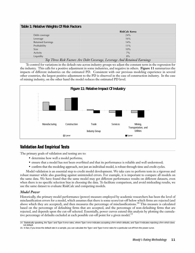
Appendix A: Testing MetricsA power curve31 is constructed by plotting, for each score, m, the proportion of defaults with a score worse than32 m,against the proportion of all firms with a score worse than m. In order to plot the power curve for a model, one shoulddo the following:

• Score all the firms with the model.

• For each score, m, calculate the percentage of all firms with scores worse than m - this is the x-axis value33.• For each score, m, calculate the percentage of defaulted firms with scores worse than m - this is the y-axis value.

Thus, if a particular model or metric M, gave 5% of all firms a score worse than m, and 10% of all defaults a score worsethan m, then its power curve would go through the point (0.05,0.1). This could be interpreted as meaning that if one were toreject all credits with a score in the worst 5% (based on M), then one would exclude 10% of all firms who go on to default.

If we consider a particular metric M, for which we bucket the scores into B different bins, then the height of thepower curve in a particular bin, b, would be calculated as follows:

where, power(b) is the height of the power curve in bin b and D(b) is the number of defaults in bin b.The result is Figure 18 below, which plots the power curve for a metric M (the line Power(M), which relates to the

left hand axis). In this case we rank-order the firms from risky (left) to less risky (right). This model would quickly have“excluded” most of the bad companies: a 20% exclusion of the worst companies according to the M score wouldexclude 70% of the future defaulters.

31. Also known as the CAP plot.32. Here “worse than” is taken to indicate that the firm is higher risk, i.e. more likely to default.33. We use percentage on the x-axis rather than the score output so that two models, with possibly different ranges of scores, can be compared to one another on the same data set.

Figure 18: Power Curve And Calibration Curve

power (b) = ,

ΣB

i=1D(i)

Σb

i=1D(i)

M

Default Probability

0

0.02

0.04

0.06

0.08

0.10

0%

20%

40%

60%

80%

100%

Perc

ent o

f Bad

s Exc

luded

Prob of Default-Calib(M) Percent Bads Excluded-Power(M)

Less RiskyMore Risky


Figure 18 also demonstrates the fact that a power curve, together with a default rate, implies a particular calibra-tion curve (this is plotted as Calib(M) which relates to the right hand axis). The default rate for a particular percentileis equal to the slope of the power curve at that point, multiplied by the average default rate for the sample. Thus, forany point m along a default metric:

where p is the mean probability of default, and is the slope of the power curve at point m.

Accuracy RatioWhile the graphical or tabular display of power is informative, and has the advantage of allowing one to examinepower at a variety of thresholds, it is useful to aggregate the power curve information into a single number that allowsunambiguous comparison. The metric that we use, called the Accuracy Ratio, compares the area under the powercurve for the model with the area under the random and perfect models. A more powerful model will be bowed outtowards the left, and will have a larger area, resulting in a higher accuracy ratio.

The accuracy ratio is defined as the ratio of the area between the actual model and the random model to the areabetween the perfect model and the random model (see Figure 12 in the Validation and Empirical Tests section for agraphical demonstration). Thus the perfect model would have an accuracy ratio of 100% and a random model wouldhave an accuracy ratio of 0%.

Using the area under the power curve implies that there can exist threshold levels such that a model with a smallertotal area has a momentary advantage. Thus the accuracy ratio is not a measure of global or complete dominance, justan intuitive measure of dominance on average.

It should be noted that it would be inappropriate to compare the accuracy ratios for two models on two differentdata sets, since any model tested on two different data sets will get different accuracy ratios on the data sets. The accu-racy ratio does however allow one to compare the performance of two models on the same underlying data set.

p(m) = p * ∂m∂Power (m)

,][

mmpower

∂∂ )(


Appendix B: Power Curve Construction DetailsThe testing approach is as follows. Typically we have annual financial statements for each firm until they default. If afirm defaults within 90 days of the financial statement that firm-year observation is dropped (see next paragraph forjustification). We assign a default score to each financial statement. If the difference between the default date and thefinancial statement date (days until default) is within the default window (90 to 730 days for the 1 year model and 90 to1825 days for the 5 year model) that firm-year observation is labeled a bad. Likewise, if the firm does not defaultwithin the window that firm-year observation is labeled as a good. We retain all good firm-year observations, but onlyone bad firm-year observation per firm. Specifically, we retain the earliest bad firm-year observation for each firm.Each remaining firm-year observation is then mapped into a percentile according to their score, and this collection ofpercentiles is the basis by which the power curve is created.

We exclude firms that default within 90 days of the financial statement date to avoid the misleading results thatcome from model performance over irrelevant time periods, such as 60 days after a statement date. Predicting defaultof very short horizons, such as less than 90 days, is basically useless, as very few statements are completed within thistime. Many lenders take 6 months to be confident that most of their middle market exposures have delivered their lat-est annual statements. By using defaulting firms once in the creation of a set of percentiles of defaulted firm scores, weavoid double counting firms. Double counting can also cause problems, especially with standard errors that usuallyassume independence within the sample.


Appendix C: The Relation Between RiskCalc PDs And Dot-PD Ratings And Moody’s Investor Services Long-Term Bond RatingsRiskCalc PDs and Moody’s long-term bond ratings are not directly comparable. They are two different, thoughrelated, credit risk measures. Exhibit 1 compares many aspects of the two systems side-by-side, highlighting similari-ties and differences.

Despite the important differences between RiskCalc PDs and Moody's long-term bond ratings, some users of oneor both risk nomenclatures find it helpful to compare them. Moody’s bond default study provides a basis for such acomparison. This study rigorously correlates Moody’s long-term corporate bond ratings with ex-post default fre-quency, allowing us to calculate historical average bond default rates for each rating category. By mapping a firm’s PDinto the historical average bond default rates, we create dot-PD ratings (e.g., Aaa.pd, Aa1.pd, Aa2.pd, … Caa2.pd,Caa3.pd, Ca.pd, C.pd), which facilitate comparison with long-term bond ratings. Moody’s bond default study is avail-able over Moody’s KMV’s web site at http://www.moodyskmv.com. The details of the PD mapping to historical aver-age long-term bond default rates are described in the May 2000 Special Comment, “Moody’s Default Model forPrivate Firms: RiskCalc for Private Firms,” also available from the web site.

Dot-pd ratings carry no additional information beyond PDs and are not long-term bond ratings for all of the rea-sons highlighted in Exhibit 1. They are, rather, a re-statement of the PDs and provide a shorthand nomenclature forprobabilities of default. Our clients have found that, for some purposes, communicating risk levels in terms of alpha-numeric ratings rather than probabilities is more intuitive. For example, for many, the difference between two compa-nies with 0.0075 and 0.0131 probabilities of default is not as easily understood as the difference between an A3.pdcompany and a Baa1.pd company.

While dot-pd ratings are not the same as long-term bond ratings, there is a correlation between them. The corre-lation, by construction, is not exact. Ratings, as indicated in Exhibit 1, are functions of not only PD, but also of theseverity of loss in the event of default (which incorporates key structural differences in instruments such as senior vs.subordinate, secured vs. unsecured, external supports) and an issuer’s risk of sudden, large changes in credit quality.Moody’s bond default study correlates ratings with only one of these risk dimensions, probability of default, whileholding constant the severity of loss and ignoring transition risk. For this reason, by construction, the correlationbetween the two systems is imprecise.

An analogous situation is the relationship between a person’s weight to their height and girth. There is a strongenough correlation between weight and height that we may draw the conclusion that taller people, on average, weighmore than shorter people. However, we could more accurately predict weight if we knew not only height but alsogirth. Analogously, we could more accurately predict Moody’s bond ratings if, in addition to PD, we know the severityof loss34, the transition risk, and the other differences outlined in Exhibit 1.

The intent of Moody's RiskCalc models is not to substitute or predict Moody's bond ratings. They are designed tocalculate expected probabilities of default for defined time horizons. The output of these models, combined with correla-tion estimates, will facilitate quantification of risk at the obligor and portfolio level. In contrast to PDs, which are pro-duced by a formula that relates information in selected financial ratios to probabilities of default, Moody's analyst ratingsare based on a more flexible and focused review of qualitative and quantitative factors, distilled by an analyst (and ratingcommittee) with sectoral expertise and in-depth understanding of an issuer’s competitive position and strategic direction.

Despite the structural difficulties in directly comparing PDs with long-term bond ratings, many of our customerswill find the systems complementary and valuable in different ways as part of a risk management solution.

Exhibit 1: Similarities & Differences Between RiskCalc PDs And Moody’s Long-Term Bond RatingsCharacteristic RiskCalc PDs Moody's Long-Term Bond RatingsUnit of Study Obligor Obligation and/or ObligorTime Horizon Specific, one or five years Non-specific, long termRisk Dimension One dimensional: Probability of default Multi-dimensional: Probability of default, severity of default & transition riskInformation Requirements Large, reliable, electronic datasets Robust to poor quality or missing dataVolatility High Low - maintained through the cycleCost Low HighSupport Technical Technical + Analyst contact & insightScale Continuous/Absolute 21 Risk Buckets/RelativeStructure Simple, codified analysis of few variables Flexible as situation may require

34. The severity of loss can be captured through use of LossCalc, another Moody’s KMV product, which provides a measure of the expected loss in the event of default.


References

Altman, E.I., 1968, Financial Ratios, Discriminant Analysis, and the Prediction of Corporate Bankruptcy, Journal of Finance 23.

Falkenstein, E., L.V. Carty, and A.K. Boral, 2000, RiskCalc for Private Companies: Moody’s Default Model, Moody’s Risk Management Services - Special Comment, May.

Falkenstein, E., A.K. Boral, and A.E. Kocagil, 2000, RiskCalc for Private Companies: Australia, Moody’s Risk Management Services - Special Comment, December.

Gupton, G., D. Gates, and L.V. Carty, 2000, Bank Loan Loss Given Default, Moody’s Investors Service Special Comment, November.

Neter, J., W. Wasserman, and M.H. Kutner, 1985 Applied Linear Statistical Models: Regression, Analysis of Variance, and Experimental Design.

Sobehart, J.R., S.C. Keenan, and R. Stein, 2000, Benchmarking Quantitative Default Risk Models: A Validation Methodology, Moody’s Investors Service Special Comment, March.

Stein, R., 2002, Benchmarking Default Prediction Models: Pitfalls and Remedies in Model Validation, Moody’s KMV, Technical Report, June.

Stein, R., A. E. Kocagil, J. Bonn and J. Akhavein, 2003, Systematic And Idiosyncratic Risk In Middle-Market Default Prediction: A Study Of The RiskCalc™ And PFM™ Models, February.

Woolridge, J.M., 2000, Introductory Econometrics: A Modern Approach, South Western.


© Copyright 2003, Moody’s Investors Service, Inc. and/or its licensors including Moody’s Assurance Company, Inc. (together, “MOODY’S”). All rights reserved. ALL INFORMATION CON-TAINED HEREIN IS PROTECTED BY COPYRIGHT LAW AND NONE OF SUCH INFORMATION MAY BE COPIED OR OTHERWISE REPRODUCED, REPACKAGED, FURTHER TRANSMIT-TED, TRANSFERRED, DISSEMINATED, REDISTRIBUTED OR RESOLD, OR STORED FOR SUBSEQUENT USE FOR ANY SUCH PURPOSE, IN WHOLE OR IN PART, IN ANY FORM ORMANNER OR BY ANY MEANS WHATSOEVER, BY ANY PERSON WITHOUT MOODY’S PRIOR WRITTEN CONSENT. All information contained herein is obtained by MOODY’S fromsources believed by it to be accurate and reliable. Because of the possibility of human or mechanical error as well as other factors, however, such information is provided “as is” without war-ranty of any kind and MOODY’S, in particular, makes no representation or warranty, express or implied, as to the accuracy, timeliness, completeness, merchantability or fitness for any partic-ular purpose of any such information. Under no circumstances shall MOODY’S have any liability to any person or entity for (a) any loss or damage in whole or in part caused by, resultingfrom, or relating to, any error (negligent or otherwise) or other circumstance or contingency within or outside the control of MOODY’S or any of its directors, officers, employees or agents inconnection with the procurement, collection, compilation, analysis, interpretation, communication, publication or delivery of any such information, or (b) any direct, indirect, special, con-sequential, compensatory or incidental damages whatsoever (including without limitation, lost profits), even if MOODY’S is advised in advance of the possibility of such damages, resultingfrom the use of or inability to use, any such information. The credit ratings, if any, constituting part of the information contained herein are, and must be construed solely as, statements ofopinion and not statements of fact or recommendations to purchase, sell or hold any securities. NO WARRANTY, EXPRESS OR IMPLIED, AS TO THE ACCURACY, TIMELINESS, COMPLETE-NESS, MERCHANTABILITY OR FITNESS FOR ANY PARTICULAR PURPOSE OF ANY SUCH RATING OR OTHER OPINION OR INFORMATION IS GIVEN OR MADE BY MOODY’S INANY FORM OR MANNER WHATSOEVER. Each rating or other opinion must be weighed solely as one factor in any investment decision made by or on behalf of any user of the informationcontained herein, and each such user must accordingly make its own study and evaluation of each security and of each issuer and guarantor of, and each provider of credit support for, eachsecurity that it may consider purchasing, holding or selling. Pursuant to Section 17(b) of the Securities Act of 1933, MOODY’S hereby discloses that most issuers of debt securities (includingcorporate and municipal bonds, debentures, notes and commercial paper) and preferred stock rated by MOODY’S have, prior to assignment of any rating, agreed to pay to MOODY’S forappraisal and rating services rendered by it fees ranging from $1,500 to $1,500,000.


To order reprints of this report (100 copies minimum), please call 1.212.553.1658.

Report Number: 78121

Authors Production Specialist

Ahmet E. Kocagil John TzanosAlexander Reyngold

moody's riskcalc™ for private companies: korea · for estimating firm default probabilities...

Documents