moore 1966
TRANSCRIPT

8/6/2019 Moore 1966
http://slidepdf.com/reader/full/moore-1966 1/234

8/6/2019 Moore 1966
http://slidepdf.com/reader/full/moore-1966 2/234
Introduction to
INTERVAL ANALYSIS
Ramon E. MooreWorthington, Ohio
R. Baker KearfottUniversity of Louisiana at Lafayette
Lafayette, Louisiana
Michael J. Cloud
Lawrence Technological UniversitySouthfield, Michigan
Society for Industrial and Applied Mathematics
Philadelphia
8/6/2019 Moore 1966
http://slidepdf.com/reader/full/moore-1966 3/234
Copyright © 2009 by the Society for Industrial and Applied Mathematics
10 9 8 7 6 5 4 3 2 1
All rights reserved. Printed in the United States of America. No part of this book may be reproduced, stored,
or transmitted in any manner without the written permission of the publisher. For information, write to
the Society for Industrial and Applied Mathematics, 3600 Market Street, 6th Floor, Philadelphia, PA,
19104-2688 USA.
Trademarked names may be used in this book without the inclusion of a trademark symbol. These names are
used in an editorial context only; no infringement of trademark is intended.
COSY INFINITY is copyrighted by the Board of Trustees of Michigan State University.
GlobSol is covered by the Boost Software License Version 1.0, August 17th, 2003. Permission is hereby
granted, free of charge, to any person or organization obtaining a copy of the software and accompanying
documentation covered by this license (the “Software”) to use, reproduce, display, distribute, execute, andtransmit the Software, and to prepare derivative works of the software, and to permit third-parties to whom
the Software is furnished to do so, all subject to the following:
The copyright notices in the Software and this entire statement, including he above license grant, thisrestriction and the following disclaimer, must be included in all copies of the Software, in whole or in part,
and all derivative works of the Software, unless such copies or derivative works are solely in the form of
machine-executable object code generated by a source language processor.
THE SOFTWARE IS PROVIDED “AS IS”, WITHOUT WARRANTY OF ANY KIND, EXPRESS OR IMPLIED, INCLUDING BUT
NOT LIMITED TO THE WARRANTIES OF MERCHANTABILITY, FITNESS FOR A PARTICULAR PURPOSE, TITLE AND
NON-INFRINGEMENT. IN NO EVENT SHALL THE COPYRIGHT HOLDERS OR ANYONE DISTRIBUTING THE SOFTWARE
BE LIABLE FOR ANY DAMAGES OR OTHER LIABILITY, WHETHER IN CONTRACT, TORT OR OTHERWISE, ARISING
FROM, OUT OF OR IN CONNECTION WITH THE SOFTWARE OR THE USE OR OTHER DEALINGS IN THE SOFTWARE.
INTLAB is copyrighted © 1998-2008 by Siegfried M. Rump @ TUHH, Institute for Reliable Computing.
Linux is a registered trademark of Linus Torvalds.Mac OS is a trademark of Apple Computer, Inc., registered in the United States and other countries. Introduction to Interval Analysis is an independent publication and has not been authorized, sponsored,
or otherwise approved by Apple Computer, Inc.
Maple is a registered trademark of Waterloo Maple, Inc.
Mathematica is a registered trademark of Wolfram Research, Inc.
MATLAB is a registered trademark of The MathWorks, Inc. For MATLAB product information, please contact
The MathWorks, Inc., 3 Apple Hill Drive, Natick, MA 01760-2098 USA, 508-647-7000, Fax: 508-647-7001,[email protected], www.mathworks.com.
Windows is a registered trademark of Microsoft Corporation in the United States and/or other countries.
Library of Congress Cataloging-in-Publication Data
Moore, Ramon E.
Introduction to interval analysis / Ramon E. Moore, R. Baker Kearfott, Michael J. Cloud.
p. cm.
Includes bibliographical references and index.
ISBN 978-0-898716-69-6
1. Interval analysis (Mathematics) I. Kearfott, R. Baker. II. Cloud, Michael J. III. Title.
QA297.75.M656 2009
511’.42—dc22
2008042348
is a registered trademark.

8/6/2019 Moore 1966
http://slidepdf.com/reader/full/moore-1966 4/234
Contents
Preface ix
1 Introduction 1
1.1 Enclosing a Solution . . . . . . . . . . . . . . . . . . . . . . . . . . . 1
1.2 Bounding Roundoff Error . . . . . . . . . . . . . . . . . . . . . . . . 3
1.3 Number Pair Extensions . . . . . . . . . . . . . . . . . . . . . . . . . 5
2 The Interval Number System 7
2.1 Basic Terms and Concepts . . . . . . . . . . . . . . . . . . . . . . . . 72.2 Order Relations for Intervals . . . . . . . . . . . . . . . . . . . . . . 9
2.3 Operations of Interval Arithmetic . . . . . . . . . . . . . . . . . . . . 10
2.4 Interval Vectors and Matrices . . . . . . . . . . . . . . . . . . . . . . 14
2.5 Some Historical References . . . . . . . . . . . . . . . . . . . . . . . 16
3 First Applications of Interval Arithmetic 19
3.1 Examples . . . . . . . . . . . . . . . . . . . . . . . . . . . . . . . . . 19
3.2 Outwardly Rounded Interval Arithmetic . . . . . . . . . . . . . . . . 22
3.3 INTLAB . . . . . . . . . . . . . . . . . . . . . . . . . . . . . . . . . 22
3.4 Other Systems and Considerations . . . . . . . . . . . . . . . . . . . 28
4 Further Properties of Interval Arithmetic 31
4.1 Algebraic Properties . . . . . . . . . . . . . . . . . . . . . . . . . . . 31
4.2 Symmetric Intervals . . . . . . . . . . . . . . . . . . . . . . . . . . . 33
4.3 Inclusion Isotonicity of Interval Arithmetic . . . . . . . . . . . . . . . 34
5 Introduction to Interval Functions 37
5.1 Set Images and United Extension . . . . . . . . . . . . . . . . . . . . 37
5.2 Elementary Functions of Interval Arguments . . . . . . . . . . . . . . 38
5.3 Interval-Valued Extensions of Real Functions . . . . . . . . . . . . . 42
5.4 The Fundamental Theorem and Its Applications . . . . . . . . . . . . 45
5.5 Remarks on Numerical Computation . . . . . . . . . . . . . . . . . . 49
6 Interval Sequences 51
6.1 A Metric for the Set of Intervals . . . . . . . . . . . . . . . . . . . . . 51
6.2 Refinement . . . . . . . . . . . . . . . . . . . . . . . . . . . . . . . . 53
v

8/6/2019 Moore 1966
http://slidepdf.com/reader/full/moore-1966 5/234
vi Contents
6.3 Finite Convergence and Stopping Criteria . . . . . . . . . . . . . . . . 57
6.4 More Efficient Refinements . . . . . . . . . . . . . . . . . . . . . . . 64
6.5 Summary . . . . . . . . . . . . . . . . . . . . . . . . . . . . . . . . . 83
7 Interval Matrices 85
7.1 Definitions . . . . . . . . . . . . . . . . . . . . . . . . . . . . . . . . 85
7.2 Interval Matrices and Dependency . . . . . . . . . . . . . . . . . . . 86
7.3 INTLAB Support for Matrix Operations . . . . . . . . . . . . . . . . 87
7.4 Systems of Linear Equations . . . . . . . . . . . . . . . . . . . . . . 88
7.5 Linear Systems with Inexact Data . . . . . . . . . . . . . . . . . . . . 927.6 More on Gaussian Elimination . . . . . . . . . . . . . . . . . . . . . 100
7.7 Sparse Linear Systems Within INTLAB . . . . . . . . . . . . . . . . 101
7.8 Final Notes . . . . . . . . . . . . . . . . . . . . . . . . . . . . . . . . 103
8 Interval Newton Methods 105
8.1 Newton’s Method in One Dimension . . . . . . . . . . . . . . . . . . 105
8.2 The Krawczyk Method . . . . . . . . . . . . . . . . . . . . . . . . . 116
8.3 Safe Starting Intervals . . . . . . . . . . . . . . . . . . . . . . . . . . 121
8.4 Multivariate Interval Newton Methods . . . . . . . . . . . . . . . . . 123
8.5 Concluding Remarks . . . . . . . . . . . . . . . . . . . . . . . . . . 127
9 Integration of Interval Functions 129
9.1 Definition and Properties of the Integral . . . . . . . . . . . . . . . . 129
9.2 Integration of Polynomials . . . . . . . . . . . . . . . . . . . . . . . 133
9.3 Polynomial Enclosure, Automatic Differentiation . . . . . . . . . . . 135
9.4 Computing Enclosures for Integrals . . . . . . . . . . . . . . . . . . . 141
9.5 Further Remarks on Interval Integration . . . . . . . . . . . . . . . . 145
9.6 Software and Further References . . . . . . . . . . . . . . . . . . . . 147
10 Integral and Differential Equations 149
10.1 Integral Equations . . . . . . . . . . . . . . . . . . . . . . . . . . . . 149
10.2 ODEs and Initial Value Problems . . . . . . . . . . . . . . . . . . . . 151
10.3 ODEs and Boundary Value Problems . . . . . . . . . . . . . . . . . . 156
10.4 Partial Differential Equations . . . . . . . . . . . . . . . . . . . . . . 156
11 Applications 157
11.1 Computer-Assisted Proofs . . . . . . . . . . . . . . . . . . . . . . . . 157
11.2 Global Optimization and Constraint Satisfaction . . . . . . . . . . . . 159
11.2.1 A Prototypical Algorithm . . . . . . . . . . . . . . . . . 159
11.2.2 Parameter Estimation . . . . . . . . . . . . . . . . . . . 161
11.2.3 Robotics Applications . . . . . . . . . . . . . . . . . . . 16211.2.4 Chemical Engineering Applications . . . . . . . . . . . . 163
11.2.5 Water Distribution Network Design . . . . . . . . . . . . 164
11.2.6 Pitfalls and Clarifications . . . . . . . . . . . . . . . . . 164
11.2.7 Additional Centers of Study . . . . . . . . . . . . . . . . 167
11.2.8 Summary of Links for Further Study . . . . . . . . . . . 168

8/6/2019 Moore 1966
http://slidepdf.com/reader/full/moore-1966 6/234
Contents vii
11.3 Structural Engineering Applications . . . . . . . . . . . . . . . . . . . 168
11.4 Computer Graphics . . . . . . . . . . . . . . . . . . . . . . . . . . . 169
11.5 Computation of Physical Constants . . . . . . . . . . . . . . . . . . . 169
11.6 Other Applications . . . . . . . . . . . . . . . . . . . . . . . . . . . . 170
11.7 For Further Study . . . . . . . . . . . . . . . . . . . . . . . . . . . . 170
A Sets and Functions 171
B Formulary 177
C Hints for Selected Exercises 185
D Internet Resources 195
E INTLAB Commands and Functions 197
References 201
Index 219

8/6/2019 Moore 1966
http://slidepdf.com/reader/full/moore-1966 7/234
8/6/2019 Moore 1966
http://slidepdf.com/reader/full/moore-1966 8/234
Preface
This book is intended primarily for those not yet familiar with methods for computing
with intervals of real numbers and what can be done with these methods.
Using a pair [a, b] of computer numbers to represent an interval of real numbers
a ≤ x ≤ b, we define an arithmetic for intervals and interval valued extensions of functions
commonlyused in computing. In this way, an interval [a, b] has a dualnature. Itis a new kind
of number pair, and it represents a set [a, b] = {x : a ≤ x ≤ b}. We combine set operations
on intervals with interval function evaluations to get algorithms for computing enclosures
of sets of solutions to computational problems. A procedure known as outward rounding
guarantees that these enclosures are rigorous, despite the roundoff errors that are inherent
in finite machine arithmetic. With interval computation we can program a computer to find
intervals that contain—with absolute certainty—the exact answers to various mathematical
problems. In effect, interval analysis allows us to compute with sets on the real line.
Interval vectors give us sets in higher-dimensional spaces. Using multinomials with interval
coefficients, we can compute with sets in function spaces.
In applications, interval analysis provides rigorous enclosures of solutions to model
equations. In this way we can at least know for sure what a mathematical model tells
us, and, from that, we might determine whether it adequately represents reality. Without
rigorous bounds on computational errors, a comparison of numerical results with physical
measurements does not tell us how realistic a mathematical model is.
Methods of computational error control, based on order estimates for approximation
errors, are not rigorous—nor do they take into account rounding error accumulation. Linear
sensitivity analysis is not a rigorous way to determine the effects of uncertainty in initial
parameters. Nor are Monte Carlo methods, based on repetitive computation, sampling
assumed density distributions for uncertain inputs. We will not go into interval statistics
here or into the use of interval arithmetic in fuzzy set theory.
By contrast, interval algorithms are designed to automatically provide rigorous bounds
on accumulated rounding errors, approximation errors, and propagated uncertainties in
initial data during the course of the computation.
Practical application areas include chemical and structural engineering, economics,
control circuitry design, beam physics, global optimization, constraint satisfaction, asteroidorbits, robotics, signal processing, computer graphics, and behavioral ecology.
Interval analysis has been used in rigorous computer-assisted proofs, for example,
Hales’ proof of the Kepler conjecture.
An interval Newton method has been developed for solving systems of nonlinear equa-
tions. While inheriting the local quadratic convergence properties of the ordinary Newton
ix
8/6/2019 Moore 1966
http://slidepdf.com/reader/full/moore-1966 9/234
x Preface
method, the interval Newton method can be used in an algorithm that is mathematically
guaranteed to find all roots within a given starting interval.
Interval analysis permits us to compute interval enclosures for the exact values of
integrals. Interval methods can bound the solutions of linear systems with inexact data.
There are rigorous interval branch-and-bound methods for global optimization, constraint
satisfaction, and parameter estimation problems.
The book opens with a brief chapter intended to get the reader into a proper mindset
for learning interval analysis. Hence its main purpose is to provide a bit of motivation and
perspective. Chapter 2 introduces the interval number system and defines the set operations
(intersection and union) and arithmetic operations (addition, subtraction, multiplication,and division) needed to work within this system.
The first applications of interval arithmetic appear in Chapter 3. Here we introduce
outward rounding and demonstrate how interval computation can automatically handle
the propagation of uncertainties all the way through a lengthy numerical calculation. We
also introduce INTLAB, a powerful and flexible MATLAB toolbox capable of performing
interval calculations.
In Chapter 4, some further properties of interval arithmetic are covered. Here the
reader becomes aware that not all the familiar algebraic properties of real arithmetic carry
over to interval arithmetic. Interval functions—residing at the heart of interval analysis—are
introduced in Chapter 5. Chapter 6 deals with sequences of intervals and interval functions,
material needed as preparation for the iterative methods to be treated in Chapter 7 (on
matrices) and Chapter 8 (on root finding). Chapter 9 is devoted to integration of interval
functions, with an introduction to automatic differentiation, an important tool in its own
right. Chapter 10 treats integral and differential equations. Finally, Chapter 11 introduces
an array of applications including several of those (optimization, etc.) mentioned above.
Various appendices serve to round out the book. Appendix A offers a brief review
of set and function terminology that may prove useful for students of engineering and the
sciences. Appendix B, the quick-reference Formulary, provides a convenient handbook-
style listing of major definitions, formulas, and results covered in the text. In Appendix C
we include hints and answers for most of the exercises that appear throughout the book.
Appendix D discusses Internet resources (such as additional reading material and software
packages—most of them freely available for download) relevant to interval computation.
Finally, Appendix E offers a list of INTLAB commands.
Research, development, and application of interval methods is now taking place in
many countries around the world, especially in Germany, but also in Austria, Belgium,
Brazil, Bulgaria, Canada, China, Denmark, Finland, France, Hungary, India, Japan, Mexico,
Norway, Poland, Spain, Sweden, Russia, the UK, and the USA. There are published works
in many languages. However, our references are largely to those in English and German,
with which the authors are most familiar. We cannot provide a comprehensive bibliography
of publications, but we have attempted to include at least a sampling of works in a broad
range of topics.The assumed background for the first 10 chapters is basic calculus plus some famil-
iarity with the elements of scientific computing. The application topics of Chapter 11 may
require a bit more background, butan attempt hasbeen made to keep much of the presentation
accessible to the nonspecialist, including senior undergraduates or beginning graduate stu-
dents in engineering, the sciences (physical, biological, economic, etc.), and mathematics.
8/6/2019 Moore 1966
http://slidepdf.com/reader/full/moore-1966 10/234
Preface xi
Of the various interval-based software packages that are available, we chose INTLAB
for several reasons. It is fully integrated into the interactive, programmable, and highly
popular MATLAB system. It is carefully written, with all basic interval computations
represented. Finally, both MATLAB and INTLAB code can be written in a fashion that is
clear and easy to debug.
We wish to cordially thank George Corliss, Andreas Frommer, and Siegfried Rump,
as well as the anonymous reviewers, for their many constructive comments. We owe
Siegfried Rump additional thanks for developing INTLAB and granting us permission to
use it in this book. Edward Rothwell and Mark Thompson provided useful feedback on
the manuscript. We are deeply grateful to the staff of SIAM, including Senior AcquisitionsEditor Elizabeth Greenspan, Developmental Editor Sara J. Murphy, Managing Editor Kelly
Thomas, Production Manager Donna Witzleben, Production Editor Ann Manning Allen,
Copy Editor Susan Fleshman, and Graphic Designer Lois Sellers.
The book is dedicated to our wives: Adena, Ruth, and Beth.
Ramon E. Moore
R. Baker Kearfott
Michael J. Cloud

8/6/2019 Moore 1966
http://slidepdf.com/reader/full/moore-1966 11/234
8/6/2019 Moore 1966
http://slidepdf.com/reader/full/moore-1966 12/234
Chapter 1
Introduction
1.1 Enclosing a Solution
In elementary mathematics, a problem is “solved” when we write down an exact solution.
We solve the equation
x
2 + x − 6 = 0
by factoring and obtaining the roots x1 = −3 and x2 = +2. Few high school algebra
teachers would be satisfied with an answer of the form
One root lies between −4 and −2, while the other lies between 1 and 3.
We need not look far, however, to find even elementary problems where answers of precisely
this form are appropriate. The quadratic equation
x2 − 2 = 0
has the positive solution √ 2. We understand that there is more to this symbol than meetsthe eye; the number it designates cannot be represented exactly with a finite number of
digits. Indeed, the notion of irrational number entails some process of approximation from
above and below. Archimedes (287–212BCE) was able to bracket π by taking a circle and
considering inscribed and circumscribed polygons. Increasing the numbers of polygonal
sides, he obtained both an increasing sequence of lower bounds and a decreasing sequence
of upper bounds for this irrational number.
Exercise 1.1. Carry out the details of Archimedes’ method for a square and a hexagon.
( Note: Hints and answers to many of the exercises can be found in Appendix C.)
Aside from irrational numbers, many situations involve quantities that are not exactlyrepresentable. In machine computation, representable lower and upper bounds are required
to describe a solution rigorously. This statement deserves much elaboration; we shall return
to it later on.
The need to enclose a number also arises in the physical sciences. Since an exper-
imentally measured quantity will be known with only limited accuracy, any calculation
1
8/6/2019 Moore 1966
http://slidepdf.com/reader/full/moore-1966 13/234
2 Chapter 1. Introduction
involving this quantity must begin with inexact initial data. Newton’s law
F = ma (1.1)
permits us to solve for the acceleration a of a body exactly only when the force F and mass
m are known exactly (i.e., to unlimited decimal precision). If the latter quantities are known
only to lie in certain ranges, say,
F 0 − F ≤ F ≤ F 0 + F and
m0 − m ≤ m ≤ m0 + m,
then a can only be bounded above and below:
al ≤ a ≤ au. (1.2)
For a relation as simple as (1.1), it is easy to determine how al and au depend on F 0, m0,
F , and m.
Exercise 1.2. Carry out this derivation to find explicit bounds on a.
For more complicated relations, however, ordinary algebra can be cumbersome. The
techniques of interval analysis will render the computation of bounds routine. In fact,
interval computation was designed for machine implementation! Examples involving hand
computation will appear throughout the book, but the reader should bear in mind that this
is only for learning purposes.
In interval analysis, we phrase inequality statements in terms of closed intervals on
the real line. We think of an interval as a set of numbers, which we commonly1 represent
as an ordered pair. Instead of (1.2), for instance, we write
a ∈ [al , au] . (1.3)
We call the interval [al , au] an enclosure of a. The use of simple set notation will repay us
many times over in the book; the reader can find a review and summary of this notation in
Appendix A. Henceforth, we will prefer notation of the form (1.3) to that of (1.2). However,
it is important to keep in mind that placing a number within a closed interval is the same as
bounding it above and below.
Let us return to our discussion of scientific calculations. We noted above that mea-
surement error can give rise to uncertainty in “initial data” such as F and m in (1.1). The
general sense is that we would like to know F and m exactly so that we can get a exactly.
In other circumstances, however, we might wish to treat F and m as parameters and inten-
tionally vary them to see how a varies. Mathematically, this problem is still treated as in
Exercise 1.2, but the shift in viewpoint is evident.
We have one more comment before we end this section. The act of merely enclosing
a solution might seem rather weak. After all, it fails to yield the solution itself. While this
is true, the degree of satisfaction involved in enclosing a solution can depend strongly onthe tightness of the enclosure obtained. The hypothetical math teacher of the first paragraph
might be much happier with answers of the form
x1 ∈ [−3.001,−2.999], x2 ∈ [1.999, 2.001].
1Other representations are discussed in Chapter 3.

8/6/2019 Moore 1966
http://slidepdf.com/reader/full/moore-1966 14/234
1.2. Bounding Roundoff Error 3
In fact, it is worth noting that if we obtain something like
x ∈ [0.66666, 0.66667],
then we do know x to four places. Moreover, there are times when we can and should be
satisfied with rather loose bounds on a solution. It might be better to know that y ∈ [59, 62]
rigorously than to have an “answer” of the form y ≈ 60 with no idea of how much error
might be present. If we can compute an interval [a, b] containing an exact solution x to some
problem, then we can take the midpoint m = (a + b)/2 of the interval as an approximation
to x and have |x − m| ≤ w/2, where w = b − a is the width of the interval. Hence we
obtain both an approximate solution and error bounds on the approximation.
Exercise 1.3. A computation shows that the mass M of a certain body lies in the
interval [3.7, 3.8] kg. State an approximation for M along with error bounds on this
approximation.
1.2 Bounding Roundoff Error
The effects of finite number representation are familiar to anyone who has done scientific
computing. Rounding error, if it manages to accumulate sufficiently, can destroy a numerical
solution.The folklore surrounding this subject can be misleading. Here we will provide one
example of a computation—involving only a small number of arithmetic operations—that
already foils a scheme often thought to be adequate for estimating roundoff error. The idea
is to perform the same computation twice, using higher-precision arithmetic the second
time. The number of figures to which the two results agree is supposed to be the number of
correct figures in the first result.
Example 1.1. Consider the recursion formula
xn+1
= x2
n(n =
0,
1,
2, . . . ) ,
(1.4)
and suppose that x0 = 1 − 10−21. We seek x75. Performing the computation with 10-place
arithmetic, we obtain the approximate values
x0 = 1, x1 = 1, . . . , x75 = 1.
Using 20-place arithmetic, we obtain the same sequence of values; hence the two values of
x75 agree to all 10 places carried in the first computation. However, the exact value satisfies
x75 < 10−10.
Exercise 1.4. Verify this.
Example 1.1 illustrates that repeating a calculation with higher-precision arithmetic
and obtaining the same answer does not show that the answer is correct. The reason
was simply that x1 is not representable exactly in either 10- or 20-place arithmetic. The
next example, first given by Rump in [220], shows that the problem can occur in a more
subtle way.

8/6/2019 Moore 1966
http://slidepdf.com/reader/full/moore-1966 15/234
4 Chapter 1. Introduction
Example 1.2. Consider evaluation of f defined by
f = 333.75 b6+ a2(11a2b2
− b6− 121 b4
− 2)+ 5.5 b8+ a/(2b)
with a = 77617.0 and b = 33096.0.
Computing powers by successive multiplications on an IBM 370 system using single, dou-
ble, and extended precision (approximately 7, 16, and 33 decimal digits, respectively),
Rump obtained the following results:
single precision f = 1.17260361 . . .double precision f = 1.17260394005317847 . . .
extended precision f = 1.17260394005317863185 . . . .
The underlining indicates agreement in digits from one computation to the next. We might
be tempted to conclude that f is close to 1.172603. However, the exact result is f =
−0.827396 . . . .
Exercise 1.5. How many digits of precision are required to find the value of f in Exam-
ple 1.2 correct to six decimal digits? Can we know when we have these six digits correct?
Preliminary hint : We will discuss INTLAB in Chapter 3, after explaining machine imple-mentations of interval arithmetic. Example 3.6 gives an INTLAB program that can compute
rigorous bounds for f to a specified accuracy.
These examples make it clear that repeating a calculation with more precision does
not necessarily provide a basis for determining the accuracy of the results. In many cases2
it is true that by carrying enough places a result of arbitrarily high accuracy can be found in
any computation involving only a finite number of real arithmetic operations beginning with
exactly known real numbers. However, it is often prohibitively difficult to tell in advance of
a computation how many places must be carried to guarantee results of required accuracy.
If instead of simply computing a numerical approximation using limited-precisionarithmetic and then worrying later about the accuracy of the results, we proceed in the spirit
of the method of Archimedes to construct intervals known in advance to contain the desired
exact result, then our main concerns will be the narrowness of the intervals we obtain and
the amount of computation required to get them. The methods treated in this book will
yield for Example 1.1, for instance, an interval close to [0, 1] using only 10-place interval
arithmetic. However, they will yield an interval of arbitrarily small width containing the
exact result by carrying enough places. In this case, obviously, more than 20 places are
needed to avoid getting 1 for the value of x0.
We have chosen just two examples for illustration. There are many others in which
the results of single, double, and quadruple precision arithmetic all agree to the number of places carried but are all wrong—even in the first digit.
2There are cases in which no amount of precision can rectify a problem, such as when a final result depends on
testing exact equality between the result of a floating point computation and another floating point number. The
code “IF sin(2 · arccos(0)) == 0 THEN f = 0 ELSE f = 1” should return f = 0, but it may always return
f = 1 regardless of the precision used.

8/6/2019 Moore 1966
http://slidepdf.com/reader/full/moore-1966 16/234
1.3. Number Pair Extensions 5
1.3 Number Pair Extensions
From time to time, mathematicians have found it necessary to produce a new number system
by extending an old one. Extensions of number systems involving ordered pairs of numbers
from a given system are commonplace. The rational numbers are essentially ordered pairs
of integers m/n. The complex numbers are ordered pairs of real numbers (x,y). In each
case, arithmetic operations are defined with rules for computing the components of a pair
resulting from an arithmetic operation on a pair of pairs. For example, we use the rule
(x1, y1)+ (x2, y2) = (x1 + x2, y1 + y2)
to add complex numbers. Pairs of special form are equivalent to numbers of the original
type: for example, each complex number of the form (x, 0) is equivalent to a real number x.
In Chapter 2 we will consider another such extension of the real numbers—this time,
to the system of closed intervals.

8/6/2019 Moore 1966
http://slidepdf.com/reader/full/moore-1966 17/234

8/6/2019 Moore 1966
http://slidepdf.com/reader/full/moore-1966 18/234
Chapter 2
The Interval NumberSystem
2.1 Basic Terms and Concepts
Recall that the closed interval denoted by [a, b] is the set of real numbers given by
[a, b] = {x ∈ R : a ≤ x ≤ b}.
Although various other types of intervals (open, half-open) appear throughout mathematics,
our work will center primarily on closed intervals. In this book, the term interval will mean
closed interval.
Endpoint Notation, Interval Equality
We will adopt the convention of denoting intervals and their endpoints by capital letters.
The left and right endpoints of an interval X will be denoted by X and X, respectively.
Thus,
X =X ,X
. (2.1)
Two intervals X and Y are said to be equal if they are the same sets. Operationally, this
happens if their corresponding endpoints are equal:
X = Y if X = Y and X = Y . (2.2)
Degenerate Intervals
We say that X is degenerate if X = X. Such an interval contains a single real number x.
By convention, we agree to identify a degenerate interval [x, x] with the real number x. In
this sense, we may write such equations as
0 = [0, 0]. (2.3)
7

8/6/2019 Moore 1966
http://slidepdf.com/reader/full/moore-1966 19/234
8 Chapter 2. The Interval Number System
Intersection, Union, and Interval Hull
The intersection of two intervals X and Y is empty if either Y < X or X < Y . In this case
we let ∅ denote the empty set and write
X ∩ Y = ∅,
indicating that X and Y have no points in common. Otherwise, we may define the intersec-
tion X ∩ Y as the interval
X ∩ Y = {z : z ∈ X and z ∈ Y }
=
max{X, Y } , min{X, Y }
. (2.4)
In this latter case, the union of X and Y is also an interval:
X ∪ Y = {z : z ∈ X or z ∈ Y }
=
min{X, Y } , max{X, Y }
. (2.5)
In general, the union of two intervals is not an interval. However, the interval hull of two
intervals, defined by
X ∪ Y =
min{X, Y } , max{X, Y }
, (2.6)
is always an interval and can be used in interval computations. We have
X ∪ Y ⊆ X ∪ Y (2.7)
for any two intervals X and Y .
Example 2.1. If X = [−1, 0] and Y = [1, 2], then X ∪ Y = [−1, 2]. Although X ∪ Y
is a disconnected set that cannot be expressed as an interval, relation (2.7) still holds.
Information is lost when we replace X ∪ Y with X ∪ Y , but X ∪ Y is easier to work with,
and the lost information is sometimes not critical.
On occasion we wish to save both parts of an interval that gets split into two disjoint
intervals. This occurs with the use of the interval Newton method discussed in Chapter 8.
Importance of Intersection
Intersection plays a key role in interval analysis. If we have two intervals containing a
result of interest—regardless of how they were obtained—then the intersection, which may
be narrower, also contains the result.
Example 2.2. Suppose two people make independent measurements of the same physicalquantity q. One finds that q = 10.3 with a measurement error less than 0.2. The other
finds that q = 10.4 with an error less than 0.2. We can represent these measurements as the
intervals X = [10.1, 10.5] and Y = [10.2, 10.6], respectively. Since q lies in both, it also
lies in X ∩ Y = [10.2, 10.5]. An empty intersection would imply that at least one of the
measurements is wrong.
8/6/2019 Moore 1966
http://slidepdf.com/reader/full/moore-1966 20/234
2.2. Order Relations for Intervals 9
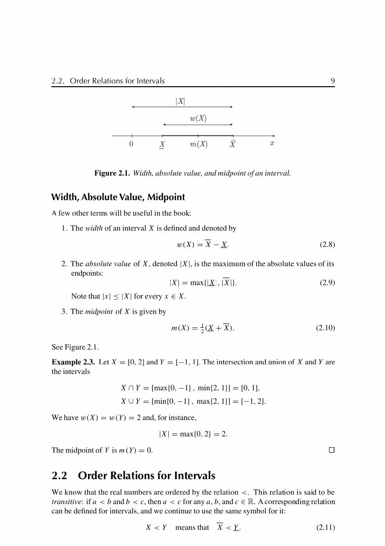
Figure 2.1. Width, absolute value, and midpoint of an interval.
Width, Absolute Value, Midpoint
A few other terms will be useful in the book:
1. The width of an interval X is defined and denoted by
w(X) = X − X. (2.8)
2. The absolute value of X, denoted |X|, is the maximum of the absolute values of its
endpoints:
|X| = max{|X|, |X|}. (2.9)
Note that |x| ≤ |X| for every x ∈ X.
3. The midpoint of X is given by
m(X) = 12
(X + X). (2.10)
See Figure 2.1.
Example 2.3. Let X = [0, 2] and Y = [−1, 1]. The intersection and union of X and Y are
the intervals
X ∩ Y = [max{0, −1} , min{2, 1}] = [0, 1],
X ∪ Y = [min{0, −1} , max{2, 1}] = [−1, 2].
We have w(X) = w(Y) = 2 and, for instance,
|X| = max{0, 2} = 2.
The midpoint of Y is m(Y) = 0.
2.2 Order Relations for IntervalsWe know that the real numbers are ordered by the relation <. This relation is said to be
transitive: if a < b and b < c, then a < c for any a, b, and c ∈ R. A corresponding relation
can be defined for intervals, and we continue to use the same symbol for it:
X < Y means that X < Y . (2.11)
8/6/2019 Moore 1966
http://slidepdf.com/reader/full/moore-1966 21/234
10 Chapter 2. The Interval Number System
For instance, [0, 1] < [2, 3], and we still have
A < B and B < C =⇒ A < C. (2.12)
Recalling the notation of (2.3), we can call X positive if X > 0 or negative if X < 0. That
is, we have X > 0 if x > 0 for all x ∈ X.
Another transitive order relation for intervals is set inclusion:
X ⊆ Y if and only if Y ≤ X and X ≤ Y . (2.13)
For example, we have [1, 3] ⊆ [0, 3]. This is a partial ordering: not every pair of intervalsis comparable under set inclusion. For example, if X and Y are overlapping intervals such
as X = [2, 5] and Y = [4, 20], then X is not contained in Y , nor is Y contained in X.
However, X ∩ Y = [4, 5], contained in both X and Y .
2.3 Operations of Interval Arithmetic
The notion of the degenerate interval permits us to regard the system of closed intervals as
an extension of the real number system. Indeed, there is an obvious one-to-one pairing
[x, x] ↔ x (2.14)
between the elements of the two systems. Let us take the next step in regarding an interval
as a new type of numerical quantity.
Definitions of the Arithmetic Operations
We are about to define the basic arithmetic operations between intervals. The key point
in these definitions is that computing with intervals is computing with sets. For example,
when we add two intervals, the resulting interval is a set containing the sums of all pairs of
numbers, one from each of the two initial sets. By definition then, the sum of two intervals
X and Y is the set
X + Y = {x + y : x ∈ X, y ∈ Y }. (2.15)
We will return to an operational description of addition momentarily (that is, to the task
of obtaining a formula by which addition can be easily carried out). But let us define the
remaining three arithmetic operations. The difference of two intervals X and Y is the set
X − Y = {x − y : x ∈ X, y ∈ Y }. (2.16)
The product of X and Y is given by
X · Y = {xy : x ∈ X, y ∈ Y }. (2.17)
We sometimes write X · Y more briefly as XY . Finally, the quotient X/Y is defined as
X/Y = {x/y : x ∈ X, y ∈ Y } (2.18)
8/6/2019 Moore 1966
http://slidepdf.com/reader/full/moore-1966 22/234
2.3. Operations of Interval Arithmetic 11
provided3 that 0 /∈ Y . Since all these definitions have the same general form, we can
summarize them by writing
X Y = {x y : x ∈ X, y ∈ Y }, (2.19)
where stands for any of the four binary operations introduced above. We could, in fact,
go further and define functions of interval variables by treating these, in a similar fashion,
as “unary operations.” That is, we can define
f(X) = {f(x) : x ∈ X}, (2.20)
where, say, f(x) = x2 or f(x) = sin x. However, we shall postpone further discussion of
interval functions until Chapter 5.
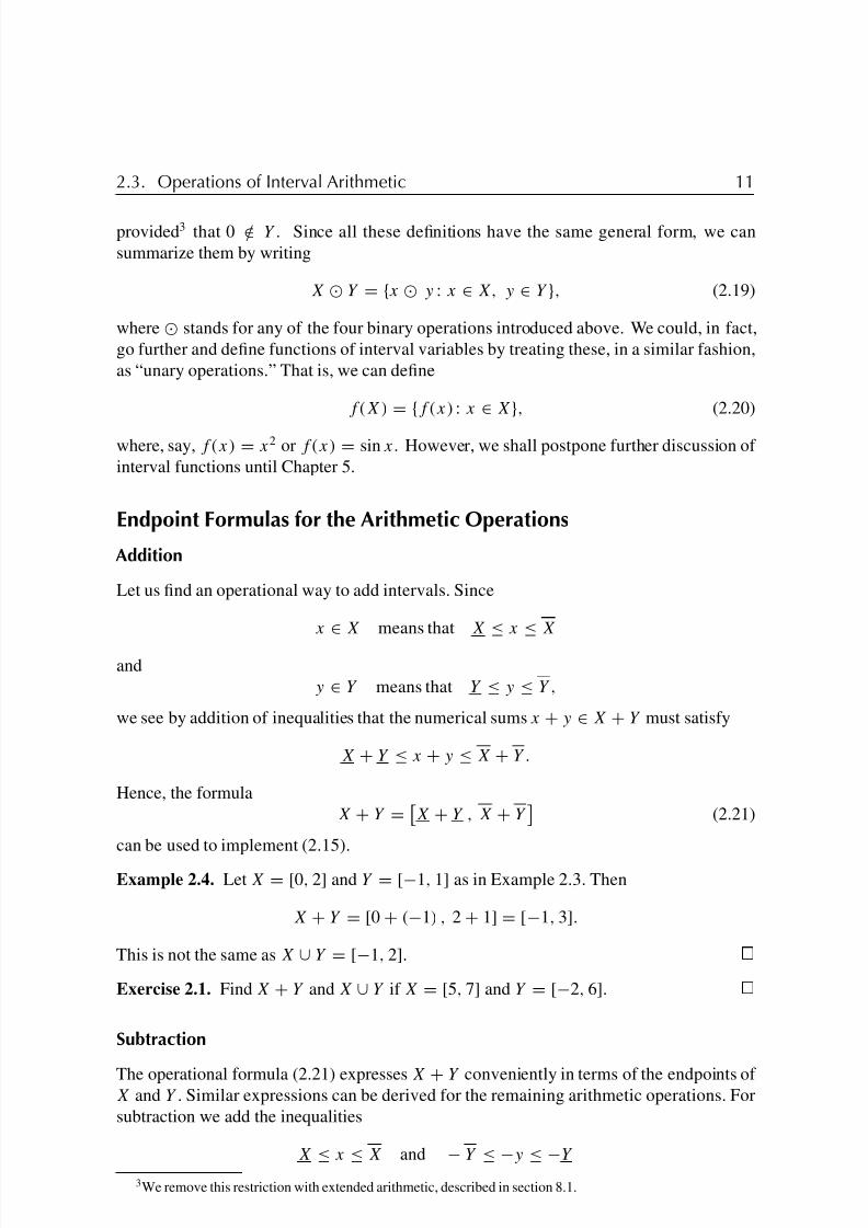
Endpoint Formulas for the Arithmetic Operations
Addition
Let us find an operational way to add intervals. Since
x ∈ X means that X ≤ x ≤ X
and
y ∈ Y means that Y ≤ y ≤ Y ,
we see by addition of inequalities that the numerical sums x + y ∈ X + Y must satisfy
X + Y ≤ x + y ≤ X + Y .
Hence, the formula
X + Y =
X + Y , X + Y
(2.21)
can be used to implement (2.15).
Example 2.4. Let X = [0, 2] and Y = [−1, 1] as in Example 2.3. Then
X + Y = [0 + (−1) , 2 + 1] = [−1, 3].
This is not the same as X ∪ Y = [−1, 2].
Exercise 2.1. Find X + Y and X ∪ Y if X = [5, 7] and Y = [−2, 6].
Subtraction
The operational formula (2.21) expresses X + Y conveniently in terms of the endpoints of X and Y . Similar expressions can be derived for the remaining arithmetic operations. For
subtraction we add the inequalities
X ≤ x ≤ X and − Y ≤ −y ≤ −Y
3We remove this restriction with extended arithmetic, described in section 8.1.

8/6/2019 Moore 1966
http://slidepdf.com/reader/full/moore-1966 23/234
12 Chapter 2. The Interval Number System
to get
X − Y ≤ x − y ≤ X − Y .
It follows that
X − Y =
X − Y , X − Y
. (2.22)
Note that
X − Y = X + (−Y ),
where
−Y =
−Y , −Y
= {y : − y ∈ Y }.
Observe the reversal of endpoints that occurs when we find the negative of an interval.
Example 2.5. If X = [−1, 0] and Y = [1, 2], then
−Y = [−2, −1]
and X − Y = X + (−Y ) = [−3, −1].
Exercise 2.2. Find X − Y if X = [5, 6] and Y = [−2, 4].
Exercise 2.3. Do we have X − X = 0 in general? Why or why not?
Multiplication
In terms of endpoints, the product X · Y of two intervals X and Y is given by
X · Y = [min S , max S ] , where S = {XY , XY , XY , XY }. (2.23)
Example 2.6. Let X = [−1, 0] and Y = [1, 2]. Then
S = {−1 · 1 , −1 · 2 , 0 · 1 , 0 · 2} = {−1 , −2 , 0}
and X · Y = [min S, max S ] = [−2, 0]. We also have, for instance, 2Y = [2, 2] · [1, 2] =
[2, 4].
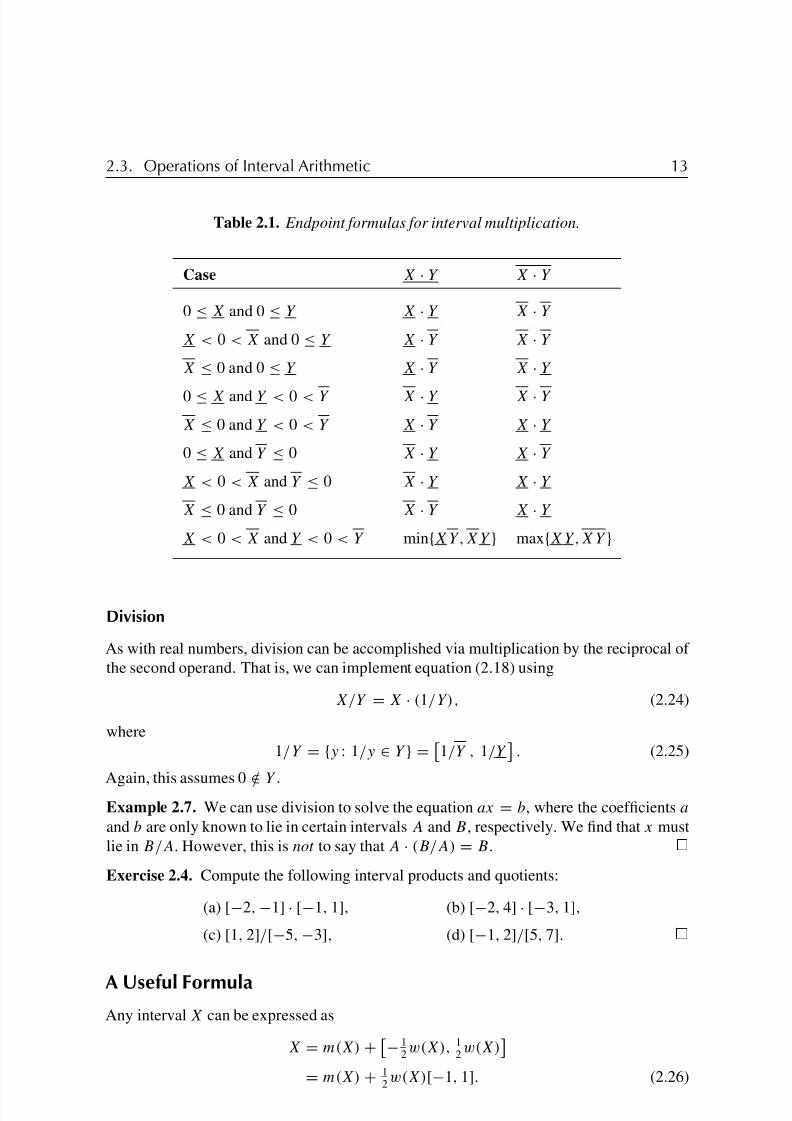
The multiplication of intervals is given in terms of the minimum and maximum of
four products of endpoints. Actually, by testing for the signs of the endpoints X, X, Y ,
and Y , the formula for the endpoints of the interval product can be broken into nine special
cases. In eight of these, only two products need be computed. The cases are shown in
Table 2.1. Whether this table, equation (2.23), or some other scheme is most efficientin an implementation of interval arithmetic depends on the programming language and
the host hardware. Before proceeding further, we briefly mention the wide availability of
self-contained interval software. Many programming languages allow interval data types
for which all necessary computational details—such as those in Table 2.1—are handled
automatically. See Appendix D for further information.
8/6/2019 Moore 1966
http://slidepdf.com/reader/full/moore-1966 24/234
2.3. Operations of Interval Arithmetic 13
Table 2.1. Endpoint formulas for interval multiplication.
Case X · Y X · Y
0 ≤ X and 0 ≤ Y X · Y X · Y
X < 0 < X and 0 ≤ Y X · Y X · Y
X ≤ 0 and 0 ≤ Y X · Y X · Y
0 ≤ X and Y < 0 < Y X · Y X · Y
X ≤ 0 and Y < 0 < Y X · Y X · Y
0 ≤ X and Y ≤ 0 X · Y X · Y
X < 0 < X and Y ≤ 0 X · Y X · Y
X ≤ 0 and Y ≤ 0 X · Y X · Y
X < 0 < X and Y < 0 < Y min{XY,XY } max{XY,XY }
Division
As with real numbers, division can be accomplished via multiplication by the reciprocal of
the second operand. That is, we can implement equation (2.18) using
X/Y = X · (1/Y), (2.24)
where
1/Y = {y : 1/y ∈ Y } =
1/Y , 1/Y
. (2.25)
Again, this assumes 0 /∈ Y .Example 2.7. We can use division to solve the equation ax = b, where the coefficients a
and b are only known to lie in certain intervals A and B, respectively. We find that x must
lie in B/A. However, this is not to say that A · (B/A) = B.
Exercise 2.4. Compute the following interval products and quotients:
(a) [−2, −1] · [−1, 1], (b) [−2, 4] · [−3, 1],
(c) [1, 2]/[−5, −3], (d) [−1, 2]/[5, 7].
A Useful Formula
Any interval X can be expressed as
X = m(X) +
− 12
w(X), 12
w(X)
= m(X) + 12
w(X)[−1, 1]. (2.26)
8/6/2019 Moore 1966
http://slidepdf.com/reader/full/moore-1966 25/234
14 Chapter 2. The Interval Number System
Example 2.8. If X = [0, 2], then by (2.26) we can write X = 1 + [−1, 1].
This idea is useful when we employ an interval to describe a quantity in terms of its
measured value m and a measurement uncertainty of no more than ±w/2:
m ± w2=
m − w
2, m + w
2
. (2.27)
2.4 Interval Vectors and Matrices
By an n-dimensional interval vector , we mean an ordered n-tuple of intervals
(X1, . . . , Xn).
We will also denote interval vectors by capital letters such as X.
Example 2.9. A two-dimensional interval vector
X = (X1, X2) =
X1, X1
,
X2, X2
can be represented as a rectangle in the x1x2-plane: it is the set of all points (x1, x2) such
that
X1 ≤ x1 ≤ X1 and X2 ≤ x2 ≤ X2.
With suitable modifications, many of the notions for ordinary intervals can be extended
to interval vectors.
1. If x = (x1, . . . , xn) is a real vector and X = (X1, . . . , Xn) is an interval vector, then
we write
x ∈ X if xi ∈ Xi for i = 1, . . . , n .
2. The intersection of two interval vectors is empty if the intersection of any of their
corresponding components is empty; that is, if Xi∩Y i = ∅ for some i, then X∩Y = ∅.
Otherwise, for X = (X1
, . . . , Xn
) and Y = (Y 1
, . . . , Y n
) we have
X ∩ Y = (X1 ∩ Y 1 , . . . , Xn ∩ Y n).
This is again an interval vector.
3. If X = (X1, . . . , Xn) and Y = (Y 1, . . . , Y n) are interval vectors, we have
X ⊆ Y if Xi ⊆ Y i for i = 1, . . . , n .
4. The width of an interval vector X = (X1, . . . , Xn) is the largest of the widths of any
of its component intervals:
w(X) = maxi
w(Xi ).
5. The midpoint of an interval vector X = (X1, . . . , Xn) is
m(X) = (m(X1) , . . . , m ( Xn)).

8/6/2019 Moore 1966
http://slidepdf.com/reader/full/moore-1966 26/234
2.4. Interval Vectors and Matrices 15
Figure 2.2. Width, norm, and midpoint of an interval vector X = (X1, X2).
6. The norm of an interval vector X = (X1, . . . , Xn) is
X = maxi
|Xi |.
This serves as a generalization of absolute value.
Example 2.10. Consider the two-dimensional constant interval vector
X = (X1, X2),
where X1 = [1, 2] and X2 = [4, 7]. We have
w(X) = max{2 − 1, 7 − 4} = 3,
m(X) =
1+22, 4+7
2
=
32, 11
2
,
andX = max { max{|1|, |2|} , max{|4|, |7|} } = max{2, 7} = 7.
These concepts are illustrated in Figure 2.2.
Example 2.10 suggests that an interval vector can be thought of as an n-dimensional
“box.” We will see applications of this idea. Any bounded set of points in n-space can be
enclosed by a union of such boxes. Furthermore, we can come arbitrarily close to a given
set of points, regardless of its geometric shape. All this leads toward the idea of computing
with sets, which can be much more general and powerful than computing with single points
(i.e., with numbers or vectors of numbers).
We can also define an inner product
P = U 1V 1 + · · · + U nV n
between two interval vectors (U 1, . . . , U n) and (V 1, . . . , V n). The interval P contains all
the real numbers defined by values of the inner product of real vectors u and v with real
components taken from the given intervals U 1, . . . , U n and V 1, . . . , V n.

8/6/2019 Moore 1966
http://slidepdf.com/reader/full/moore-1966 27/234
16 Chapter 2. The Interval Number System
Exercise 2.5. A family of Cartesian vectors is given by (f, 6,−7), where 1 ≤ f ≤ 3.
Calculate the range of inner products between these vectors and 1√ 5(1, 2, 0).
By an interval matrix we mean a mean a matrix whose elements are interval numbers.
Such matrices are covered further in Chapter 7. In particular, there are some pitfalls,
subtleties, and interesting properties of interval matrix-vector multiplication that we will
discuss there.
2.5 Some Historical References
Much of the modern literature on interval arithmetic can be traced to R. E. Moore’s disser-
tation [146], through his book [148]. A collection of early papers by Moore and coworkers
can be found on the web (see Appendix D for some starting links relevant to the material
in this section). The earlier work [238], written independently and often overlooked, also
contained many of the ideas expressed in [146]. The paper [238], as well as other early
papers dealing with similar concepts, are available on the web. Moore describes the thought
process and inspiration that led to his seminal dissertation in [155].
Other researchers began work with interval computations almost contemporary with
or shortly after (that is, within a decade of) Moore’s early work.
• Eldon Hansen investigated reliable solution of linear systems and other topics; see
[58, 59, 60, 61, 62, 67, 68], etc. A decade or so later, he began a lasting collaboration
with Bill Walster, including [69, 247]. A notable recent reference is [57].
• William Kahan, known for his work in standardization of floating point arithmetic, had
several publications on interval computations, including [87, 88, 89, 90, 91] within
several years of Moore’s dissertation. Often cited is [89] on extended arithmetic.
Kahan devised a closed system in which an interval divided by an interval containing
0 is well defined. Kahan arithmetic was originally meant for dealing with continued
fractions, a task for which it is particularly suited. It is also consistent with Kahan’s
philosophy of nonstop exception-free arithmetic, embodied in the IEEE 754 standardfor binary floating point arithmetic. In fact, some properties of the binary floating point
standard, most notably directed roundings, are important for interval computations;
others, such as operations with ∞, facilitate extended arithmetic. The details of
both the operations with ∞ in the floating point standard, as well as the details and
mathematical underpinnings of extended interval arithmetic, continue to be debated
and revised.
• Several researchers at the University of Karlsruhe started a tradition in interval com-
putation that continues to influence mathematics and computer science in Germany:
– Karl Nickel began at Karlsruhe, where he helped establish the discipline of computer science in Germany. His early publications on interval computations
include [19, 41, 175, 176, 177, 178, 179]. Nickel later moved to the Univer-
sity of Freiburg, where he supported the field with work such as editing the
Freiburger Intervallberichte preprint series, in which there are many gems,
some not published elsewhere. One researcher he encouraged at Freiburg is

8/6/2019 Moore 1966
http://slidepdf.com/reader/full/moore-1966 28/234
2.5. Some Historical References 17
Arnold Neumaier, presently at the University of Vienna. Neumaier continues
to be active in interval computations and global optimization.
– Ulrich Kulisch, starting in 1966, has been influential through his work and that
of his students. His early work includes [15, 16, 17, 18, 19, 122, 123], as well
as slightly later technical reports at the University of Wisconsin at Madison
and the IBM Thomas Watson Research Center. Many of his 49 students hold
prominent academic positions in German universities. Two of his early students
are Götz Alefeld and Jürgen Herzberger, both receiving the Ph.D. in 1969.
Alefeld’s early work includes [4, 6, 5]; he has mentored 29 Ph.D. students
and continues to hold a chair at the University of Karlsruhe. Herzberger’searly work includes his dissertation [73], [74, 75, 76, 77, 78], and a productive
collaboration with Alefeld, including [7, 8, 9, 10, 11, 14]. The most famous
fruit of this collaboration is the classic introduction to interval analysis [12],
which Jon Rokne translated into English a decade later [13]. Another student
of Kulisch is Siegfried Rump (1980), presently head of the Institute of Reliable
Computing at the Technical University of Hamburg. Rump has done work in
error bounds for solutions to linear and nonlinear systems, among other things.
He developed the INTLAB toolbox that we use throughout this book.
– Rudolf Krawczyk was at Karlsruhe in 1969 when he published [119], where the
much-studied Krawczyk method first appeared. (See section 8.2 of this work.)
• Soon after publication of Moore’s dissertation, he was invited to give a talk at a
seminar on error in digital computing at the Mathematics Research Center (MRC) at
the University of Wisconsin. The proceedings of this seminar, published as [195, 196],
were edited by Louis Rall. Moore joined MRC and wrote Interval Analysis during the
summer of 1965. Ulrich Kulisch and Karl Nickel visited the MRC, and the work in
interval analysis at the MRC continued through the 1980s, as evidenced in technical
reports such as [26, 30, 32, 124, 127, 180, 181, 182, 183, 197, 198, 199, 201, 202,
203, 204, 205, 206, 207, 208, 215, 251, 252, 253, 254, 255].
• There is early work other than at the aforementioned centers. For example, Peter
Henrici et al. have studied complex interval arithmetic, such as in [47].
We will draw upon these and more recent references throughout the book.

8/6/2019 Moore 1966
http://slidepdf.com/reader/full/moore-1966 29/234

8/6/2019 Moore 1966
http://slidepdf.com/reader/full/moore-1966 30/234

8/6/2019 Moore 1966
http://slidepdf.com/reader/full/moore-1966 31/234
20 Chapter 3. First Applications of Interval Arithmetic
Clearly, if we were to round the endpoints of A both upward by one digit to obtain
A = [1.9985003 , 2.0015003] m2,
this new interval A would not contain the value (3.2). Such an event would defeat the
entire purpose of rigorous computation! Instead, we will always implement a procedure
called outward rounding: we will round in such a way that the left endpoint moves to the
left (on the number line) and the right endpoint moves to the right. The resulting interval
contains the one we started with and hence still has a as a member. In the present example,
we could round outwardly to the nearest square millimeter and obtain the interval
A = [1.998, 2.002] m2.
The statement
1.998 m2 ≤ a ≤ 2.002 m2
is definitely true, and the ability to depend on this is essential as we proceed.
Exercise 3.1. Perform outward rounding, at the third decimal place, on the interval [1.23456,
1.45678].
Exercise 3.2. The dimensions of a rectangular box are measured as w = 7.2 ± 0.1, l =14.9 ± 0.1, and h = 405.6 ± 0.2. Find several intervals containing the volume of the
box.
Exercise 3.3. A Wien bridge electric circuit oscillates at frequency f 0 given by f 0 =
1/(2πRC) Hz. If components having nominal values C = 1 nF and R = 15 k with
manufacturing tolerances of 10% are used, in what range must f 0 lie?
Interval arithmetic also makes it easy to track the propagation of initial uncertainties
through a series of calculations.
Example 3.2. Consider the formula
V =
2gM
E(M + E)− V 0, (3.3)
which has an application discussed in [149]. Suppose we know that
g ∈ [1.32710, 1.32715](1020),
V 0 ∈ [2.929, 3.029](104),
M ∈ [2.066, 2.493](1011
),
E ∈ [1.470, 1.521](1011),
and we seek an interval containing V . The necessary calculations are laborious if done by
hand, and in Example 3.3 we will show how they can be easily done with INTLAB. It is
worth examining the final results at this time, however. We will discuss functions such as
8/6/2019 Moore 1966
http://slidepdf.com/reader/full/moore-1966 32/234
3.1. Examples 21
square roots systemically in Chapter 5, but for now it will suffice to note that if x ∈ [a, b]with a and b positive numbers such that a < b, then
√ x ∈
√ a ,
√ b
.
Carrying out the operations indicated in (3.3), we find that
V ∈ [−324, 6394]. (3.4)
The interesting part is that instead of (3.3) we can use the expression
V =
2g
E(1 + EM
)− V 0.
This is equivalent in ordinary arithmetic, but gives the sharper (i.e., narrower) result
V ∈ [1411.7, 4413.5]. (3.5)
So two expressions that are equivalent in ordinary arithmetic can fail to be equivalent in
interval arithmetic. This is a very important issue that we will continue to discuss.
Let us pursue the phenomenon of the previous example using the simpler formula
M
1 + M = 1
1 + 1M
.
For the interval data M = [14, 15], the first expression yields
[14, 15]1 + [14, 15] =
[14, 15][15, 16] =
1416
, 1515
= [0.875, 1.0]
because we divide by the largest number in the denominator to get the left endpoint of the
result. The second expression yields the sharper result
11 + 1
[14,15]= 1
1 +
115
, 114
= 11615
, 1514
= 1415
, 1516
∈ [0.933, 0.938].
The result just shown, namely, 1415
, 1516
∈ [0.933, 0.938]illustrates how we can maintain rigorous enclosure despite machine rounding error. In
decimal form, we would have the exact result,
1415
, 1516 = [0.933333 . . . , 0.9375].
However, the left endpoint is a repeating decimal and cannot be exactly represented by afinite string of digits. Since we can compute only with finite strings of digits, we maintain
rigorous enclosure of interval results through outward rounding. Sometimes no rounding is
needed, if we have the exact result in no more than the maximum number of digits allowed.
If we allow only three places, we get the result shown above. We see that [0.933, 0.938] is
the narrowest interval, using only three places, that contains the interval
1415
, 1516
.

8/6/2019 Moore 1966
http://slidepdf.com/reader/full/moore-1966 33/234
22 Chapter 3. First Applications of Interval Arithmetic
3.2 Outwardly Rounded Interval Arithmetic
In practice, outward rounding is implemented at every arithmetic operation—always at the
last digit carried. In optimal outward rounding, the outwardly rounded left endpoint is
the closest machine number less than or equal to the exact left endpoint, and the outwardly
rounded right endpoint is the closest machine number greater than or equal to the exact right
endpoint. Numerous interval software systems do this automatically (see Appendix D).
Definition 3.1. By outwardly rounded interval arithmetic (IA), we mean interval arithmetic,
implemented on a computer, with outward rounding at the last digit carried.
The classic reference on IA is the mathematically rigorous treatment by Kulisch and
Miranker [125].
3.3 INTLAB
Software packages that implement interval arithmetic use outward rounding and implement
elementary functions of interval arguments (which we will see in Chapter 5). Particularly
convenient is INTLAB, available free of charge for noncommercial use. INTLAB provides
an interactive environment within MATLAB, a commonly used interactive and program-
ming system both for academic and commercial purposes. One who has MATLAB and hasinstalled INTLAB can easily experiment with interval arithmetic.4
Example 3.3. We can use INTLAB to perform the calculations for Example 3.2. At theMATLAB prompt (>>), we begin by issuing the command
intvalinit(’DisplayInfsup’)
which directs INTLAB to display intervals using its infimum-supremum notation (or lowerbound–upper bound representation, i.e., our usual endpoint notation). After providing con-firmation5 of this default display setting, INTLAB returns to the MATLAB prompt and
awaits further instruction. We now type
>> g = infsup(1.32710e20,1.32715e20)
and hit enter; INTLAB responds (MATLAB style) with
intval g = 1.0e+020 * [ 1.3271 , 1.3272 ]
which merely confirms the value of g that we entered. We can suppress this echoing featureby appending a semicolon to the end of our variable assignment:
g = infsup(1.32710e20,1.32715e20);
Similarly, we can continue to enter the remaining values needed in Example 3.2. Ourinteractive session appears on screen as
4Many books on MATLAB are available (e.g., [79, 145, 214]). The interested reader may wish to consult one
before attempting to read further.5For brevity we omit this confirmation from our examples. MATLAB output has been lightly edited to conserve
space.
8/6/2019 Moore 1966
http://slidepdf.com/reader/full/moore-1966 34/234
3.3. INTLAB 23
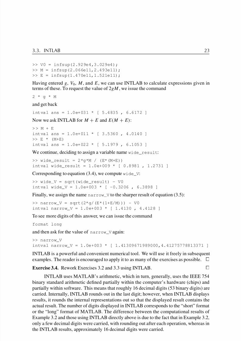
>> V0 = infsup(2.929e4,3.029e4);
>> M = infsup(2.066e11,2.493e11);
>> E = infsup(1.470e11,1.521e11);
Having entered g, V 0, M , and E, we can use INTLAB to calculate expressions given interms of these. To request the value of 2gM , we issue the command
2 * g * M
and get back
intval ans = 1.0e+031 * [ 5.4835 , 6.6172 ]
Now we ask INTLAB for M + E and E(M + E):
> > M + E
intval ans = 1.0e+011 * [ 3.5360 , 4.0140 ]
>> E * (M+E)
intval ans = 1.0e+022 * [ 5.1979 , 6.1053 ]
We continue, deciding to assign a variable name wide_result:
>> wide_result = 2*g*M / (E*(M+E))
intval wide_result = 1.0e+009 * [ 0.8981 , 1.2731 ]
Corresponding to equation (3.4), we compute wide_V:
>> wide_V = sqrt(wide_result) - V0
intval wide_V = 1.0e+003 * [ -0.3206 , 6.3898 ]
Finally, we assign the name narrow_V to the sharper result of equation (3.5):
>> narrow_V = sqrt(2*g/(E*(1+E/M))) - V0
intval narrow_V = 1.0e+003 * [ 1.4130 , 4.4128 ]
To see more digits of this answer, we can issue the command
format long
and then ask for the value of narrow_V again:
>> narrow_Vintval narrow_V = 1.0e+003 * [ 1.41309671989000,4.41275778813371 ]
INTLAB is a powerful and convenient numerical tool. We will use it freely in subsequent
examples. The reader is encouraged to apply it to as many of the exercises as possible.
Exercise 3.4. Rework Exercises 3.2 and 3.3 using INTLAB.
INTLAB uses MATLAB’s arithmetic, which in turn, generally, uses the IEEE 754
binary standard arithmetic defined partially within the computer’s hardware (chips) and
partially within software. This means that roughly 16 decimal digits (53 binary digits) are
carried. Internally, INTLAB rounds out in the last digit; however, when INTLAB displays
results, it rounds the internal representations out so that the displayed result contains theactual result. The number of digits displayed in INTLAB corresponds to the “short” format
or the “long” format of MATLAB. The difference between the computational results of
Example 3.2 and those using INTLAB directly above is due to the fact that in Example 3.2,
only a few decimal digits were carried, with rounding out after each operation, whereas in
the INTLAB results, approximately 16 decimal digits were carried.

8/6/2019 Moore 1966
http://slidepdf.com/reader/full/moore-1966 35/234
24 Chapter 3. First Applications of Interval Arithmetic
Example 3.4. The following MATLAB/INTLAB computations illustrate the display of intervals in INTLAB.
>> format short
>> rx = 2/3
rx = 0.6667
>> format long
>> rx
rx = 0.666666666666667
>> format short
>> intvalinit(’DisplayInfsup’)
===> Default display of intervals by infimum/supremum
>> x = infsup(2/3,2/3)
intval x = [ 0.6666 , 0.6667 ]
>> format long
>> x
intval x = [ 0.66666666666666 , 0.66666666666667 ]
In these computations, when 2/3 is entered into MATLAB, it is converted (presumably6)
to the closest IEEE double precision binary number to 2/3 and stored in rx. When rx
is printed, this binary number is converted back to a decimal number, according to the
format (short or long) in effect when the output is requested. When the INTLAB commandx = midrad(2/3,0) is issued, an internal representation7 corresponding to an interval
whose lower bound is less than 2/3 (a number that is not exactly representable in any binary
format) and whose upper bound is greater than 2/3 is generated. The lower bound and upper
bound are very close together in this case, possibly with no binary numbers in the system
between. When output in the short format, the decimal representation of the lower bound is
produced to be smaller than or equal to the exact lower bound of the stored binary interval,
and the decimal representation of the upper bound is greater than or equal to the exact upper
bound of the stored binary interval. Thus, the output interval is wider in the short format
than in the long format, but, in any case, the output will always contain the exact value 2/3.
INTLAB provides a special syntax for mathematically rigorous enclosures of decimalnumbers that are entered. For example, one may obtain a mathematically rigorous enclosurefor the interval [1.32710 × 10²⁰, 1.32715 × 10²⁰] from Example 3.3 with the followingMATLAB dialogue:
>> g = hull(intval(’1.32710e20’),intval(’1.32715e20’))
intval g = 1.0e+020 * [ 1.3271 , 1.3272 ]
The following MATLAB m-file8 could also be used:
function [ivl] = rigorinfsup(x,y)
% [ivl] = rigorinfsup(x,y) returns an interval whose internal
% representation contains a rigorous enclosure for the
% decimal strings x and y. It is an error to call this function
6We have not verified this on all systems for all inputs.7The representation is not necessarily in terms of lower bound andupper bound, but maybe in terms of midpoint
and radius.8An m-file is essentially a MATLAB program. Appendix D contains instructions on how to obtain the m-files
used in this book. We will say more about m-files later.

8/6/2019 Moore 1966
http://slidepdf.com/reader/full/moore-1966 36/234
3.3. INTLAB 25
% if the arguments are not character.
if (ischar(x) & ischar(y))
ilower = intval(x);
iupper = intval(y);
ivl = infsup(inf(ilower), sup(iupper));
else
display(’Error in rigorinfsup; one of arguments is not’);
display(’a character string.’);
ivl = infsup(-Inf, Inf);
end;
Use of rigorinfsup is exemplified in the following short MATLAB dialogue:
>> g = rigorinfsup(’1.32710e20’,’1.32715e20’)
intval g = 1.0e+020 * [ 1.3271 , 1.3272 ]
Above, the output of rigorinfsup is given in short format. This is the default format
when MATLAB starts, unless the format long command has previously been issued in
the startup.m script or elsewhere in the session.
Caution There is a reason for this special syntax with quotation marks.9 In particu-
lar, we should mention a subtle aspect of INTLAB and other languages implementinginterval arithmetic in a similar way.10 The problem is that when one enters a constant
in decimal form, such as 1.32710e20, the system needs to convert this constant into
its internal binary format for further use. However, unless the constant is representable
as a fraction whose denominator is a power of 2, there is no internal binary number
that corresponds exactly to the decimal number that was entered. The conversion is
to a binary number that is near to the decimal number but is not guaranteed to be less
than or greater than the corresponding decimal number. Thus, issuing the command g =
infsup(1.32710e20,1.32715e20) in MATLAB results in an internally stored binary in-
terval for g that may not contain the decimal interval [1.32710×10²⁰, 1.32715×10²⁰]. This
discrepancy usually is not noticed but occasionally causes unexpected results. In contrast,
when one uses infsup(’1.32710e20’,’1.32715e20’), INTLAB provides a conver-
sion with rigorous rounding. For example, the internal representation for intval(0.1) or
infsup(0.1,0.1) does not necessarily include the exact value 0.1, but intval(’0.1’)
does.11
Three representations for intervals can appear in INTLAB computations: the infimum-
supremum representation, which we have already discussed, the midpoint-radius represen-
tation, mentioned in Example 3.4, and the significant digits representation. The midpoint-
radius representation is analogous to the specification of tolerances familiar to engineers.
For example, if an electrical resistor is given by R = 10 ± 1 , then the midpoint-radius
representation of the set of values for R would be 10, 1, whereas the infimum-supremum
representation of the interval for R would be [9, 11]. (In the midpoint-radius represen-
tation, the radius is rounded up for display, to ensure that the displayed interval contains
9The quotation marks tell MATLAB that the argument is a string of characters, not a usual number. This allows
INTLAB to use a special routine to process this string.10With “operator overloading.”11infsup(’0.1’,’0.1’) does not give the expected results in INTLAB version 5.4 or earlier.

8/6/2019 Moore 1966
http://slidepdf.com/reader/full/moore-1966 37/234
26 Chapter 3. First Applications of Interval Arithmetic
the actual interval.) There are certain advantages and disadvantages to the midpoint-radius
representation, both in the display of intervals and in internal computations with intervals.
Example 3.5. Suppose an electrical resistor has a nominal value of 100 and a manufac-turing tolerance of 10%. INTLAB permits us to enter this information as follows:
>> Ohms = 100;
>> R = midrad(Ohms,0.1*Ohms)
intval R = [ 90.0000 , 110.0000 ]
Note, however, that R is still displayed in the current default mode, which is Infsup. The
command
intvalinit(’DisplayMidrad’)
will change INTLAB to Midrad mode. Now we can see
>> R
intval R = < 100.0000 , 10.0000 >
Note that we can input a “thin” interval by specifying its radius as zero or by simply notspecifying the radius:
>> thin = midrad(1,0)
intval thin = < 1.0000 , 0.0000 >
We can always switch back to Infsup mode and see thin in that notation:
>> intvalinit(’DisplayInfsup’)
>> thin
intval thin = [ 1.0000 , 1.0000 ]
The significant digits or uncertainty representation is appropriate when we are ap-proximating a single real number and wish to easily see how many digits of it are knownwith mathematical certainty. The interval is displayed as a single real number, and the lastdigit displayed is correct to within one unit. The following MATLAB dialogue gives some
examples:
>> intvalinit(’Display_’)
>> infsup(1.11,1.12)
intval ans = 1.12__
>> infsup(1.1,1.5)
intval ans = 1.____
>> infsup(1.11,1.13)
intval ans = 1.12__
>> infsup(1.1111111,1.1111112)
intval ans = 1.1111
>> format long>> infsup(1.11,1.12)
intval ans = 1.12____________
>> infsup(1.11111,1.11113)
intval ans = 1.11112_________
>> infsup(2,4)
intval ans = 1_.______________
8/6/2019 Moore 1966
http://slidepdf.com/reader/full/moore-1966 38/234
3.3. INTLAB 27
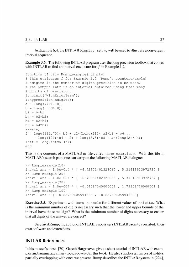
In Example 6.4, the INTLAB Display_ setting will be used to illustrate a convergent
interval sequence.
Example 3.6. The following INTLAB program uses the long precision toolbox that comeswith INTLAB to find an interval enclosure for f in Example 1.2:
function [Intf]= Rump_example(ndigits)
% This evaluates f for Example 1.2 (Rump’s counterexample)
% ndigits is the number of digits precision to be used.
% The output Intf is an interval obtained using that many
% digits of precision.
longinit(’WithErrorTerm’);
longprecision(ndigits);
a = long(77617.0);
b = long(33096.0);
b2 = b*b;
b4 = b2*b2;
b6 = b2*b4;
b8 = b4*b4;
a2=a*a;
f = long(333.75)* b6 + a2*(long(11)* a2*b2 - b6...
- long(121)*b4 - 2) + long(5.5)*b8 + a/(long(2)* b);
Intf = long2intval(f);
end
This is the contents of a MATLAB m-file called Rump_example.m. With this file inMATLAB’s search path, one can carry on the following MATLAB dialogue:
>> Rump_example(10)
intval ans = 1.0e+014 * [ -6.72351402328065 , 5.31613913972737 ]
>> Rump_example(20)
intval ans = 1.0e+014 * [ -6.72351402328065 , 5.31613913972737 ]
>> Rump_example(30)
intval ans = 1.0e+007 * [ -0.04587540000001 , 1.72359720000001 ]>> Rump_example(100)
intval ans = [ -0.82739605994683 , -0.82739605994682 ]
Exercise 3.5. Experiment with Rump_example for different values of ndigits. What
is the minimum number of digits necessary such that the lower and upper bounds of the
interval have the same sign? What is the minimum number of digits necessary to ensure
that all digits of the answer are correct?
Siegfried Rump, the author of INTLAB, encourages INTLAB users to contribute their
own software and extensions.
INTLAB References
In his master’s thesis [70], Gareth Hargreaves gives a short tutorial of INTLAB with exam-
ples and summarizes many topics covered in this book. He also supplies a number of m-files,
partially overlapping with ones we present. Rump describes the INTLAB system in [224],

8/6/2019 Moore 1966
http://slidepdf.com/reader/full/moore-1966 39/234
28 Chapter 3. First Applications of Interval Arithmetic
while extensive documentation for INTLAB is integrated into MATLAB’s “demo” system,
starting with INTLAB version 5.4. Rump describes the way interval arithmetic is imple-
mented within INTLAB in [223]. The INTLAB toolbox features prominently in the solution
of 5 of the 10 problems posed in the SIAM 100-digit challenge; 12 this is described in [27].
3.4 Other Systems and Considerations
Shin’ichi Oishi has developed SLAB, a stand-alone MATLAB-like system specifically for
interval computations and the automatic result verification it provides. It is available for
free (under the GNU license), and has builds for MS-Windows, Linux, and Mac OS. A short
description appears in [104].
Tools are available for doing interval computations within traditional programming
languages. In Fortran, there are the ACM Transactions on Mathematical Software algorithms
[101] and [96]. Various groups have also developed tools for use with C++. Prominent
among these is C-XSC [80], developed by a group of researchers associated with Ulrich
Kulisch at the University of Karlsruhe and presently supported from members of that group
at the University of Wuppertal. Extensive libraries have been developed for automatically
verified versions of standard computations in numerical analysis using C-XSC; an early
version of this toolbox is described in [56], while an update containing more advanced
algorithms is [117]. Alternate, widely used class libraries for interval arithmetic in C++ arePROFIL/BIAS [111] and FILIB++ [132]. See Appendix D.
Under certain circumstances, it may be desirable to use higher precision (i.e., more
digits) in the interval representations than is available in, say, the IEEE 754 standard for
binary floating point arithmetic. Along these lines, Nathalie Revol et al. have developed
the multiple precision interval library MPFI [217].
A major thrust by Kulisch and his students at the University of Karlsruhe has been
to develop algorithms that provide narrow intervals to rigorously enclose the solutions to
point linear systems of equations, even if these linear systems happen to be ill-conditioned.
Central to this is the concept of accurate dot product . In particular, methods for solving
and for verifying bounds on the solutions of linear systems of equations involve repeatedcomputation of dot products. If outward roundings are done after each addition and mul-
tiplication in the dot product, then the widths of the intervals can rapidly increase during
the computation, resulting in an enclosure for the dot product that is too wide to be useful.
This is especially true if there is much cancelation during the computation, something that
can happen for an ill-conditioned system, even if the components of the original vectors
are points. Kulisch has advocated a long accumulator , described in [126] among other
publications. The concept is that the sum in the dot product is stored in a register having so
many digits that, when the final result is rounded to the usual number of digits, the result is
the closest number less than or the closest number greater than the mathematically correct
result. This long accumulator has been implemented in hardware in several machines andis implemented in software in C-XSC and the other XSC languages. However, the accurate
dot product is relatively slow when implemented in software, and its necessity has been
12The SIAM 100-digit challenge was a series of 10 numerical problems posed by Nick Trefethen in which the
goal was to supply 10 correct digits. A nominal prize was given for the best answers, and the contestants took it
upon themselves to rigorously verify the correctness of the digits supplied.

8/6/2019 Moore 1966
http://slidepdf.com/reader/full/moore-1966 40/234
3.4. Other Systems and Considerations 29
controversial. Ogita et al. have proposed and analyzed methods for computing sums and
dot products accurately and quickly using standard hardware, without a long accumulator
[185]. Such algorithms do not always give a result that rounds to the nearest number to the
correct result, but, with quadruple precision13 give results that are within one or two units
of the correct result except in certain cases; Rump et al. have a formalized analysis of this.
This group has used these techniques in algorithms for verification of solutions of linear
systems [186, 189, 226].
Accurate dot products in general will not help when there is interval uncertainty
in the coefficients of the original linear system and the coefficients are assumed to vary
independently.Interval arithmetic is also available in the Mathematica [109] and Maple [37, 116]
computer algebra systems. Finally, other and older implementations of interval arithmetic
are described in [97, pp. 102–112].
13Now common and perhaps specified in the revision of the IEEE binary floating point standard.

8/6/2019 Moore 1966
http://slidepdf.com/reader/full/moore-1966 41/234

8/6/2019 Moore 1966
http://slidepdf.com/reader/full/moore-1966 42/234
Chapter 4
Further Properties of Interval Arithmetic
In Chapter 2 we introduced the definitions of the basic interval arithmetic operations. With
proper understanding of the notation, it is possible to summarize them neatly in one line:
X Y = {x y : x ∈ X, y ∈ Y }, where can be + , − , · , or / . (4.1)
(Until Chapter 8, the quotient X/Y is defined only if 0 /∈ Y .) These definitions lead to anumber of familiar looking algebraic properties. In addition, however, their set-theoretic
character implies certain important relationships involving set containment. The material
of the present chapter constitutes essential preparation for the study of interval functions in
Chapter 5 and beyond.
4.1 Algebraic Properties
Commutativity and Associativity
It is easy to show that both interval addition and multiplication are commutative and asso-ciative; we have
X + Y = Y + X, X + (Y + Z) = (X + Y ) + Z,
XY = Y X, X(Y Z) = (XY)Z
for any three intervals X, Y , and Z.
Additive and Multiplicative Identity Elements
The degenerate intervals 0 and 1 are additive and multiplicative identity elements in the
system of intervals:0 + X = X + 0 = X,
1 · X = X · 1 = X,
0 · X = X · 0 = 0
for any X.
31

8/6/2019 Moore 1966
http://slidepdf.com/reader/full/moore-1966 43/234
32 Chapter 4. Further Properties of Interval Arithmetic
Nonexistence of Inverse Elements
We caution that −X is not an additive inverse for X in the system of intervals. Indeed, we
have
X + (−X) =
X , X
+
−X , −X
=
X − X , X − X
,
and this equals [0, 0] only if X = X. If X does not have zero width, then
X − X = w(X)[−1, 1]. (4.2)
Similarly, X/X = 1 only if w(X) = 0. In general,
X/X =
X/X, X/X
if 0 < X,
X/X , X/X
if X < 0.
(4.3)
We do not have additive or multiplicative inverses except for degenerate intervals. However,
we always have the inclusions 0 ∈ X − X and 1 ∈ X/X.
Exercise 4.1. Show that X · [−1, 1] = max(|X|, |X|)[−1, 1].
Exercise 4.2. Show that if c > 0, then [c, c] ·
X , X
=
c X , c X
for any X.
Subdistributivity
The distributive law
x(y + z) = xy + xz
of ordinary arithmetic also fails to hold for intervals. An easy counterexample can be
obtained by taking X = [1, 2], Y = [1, 1], and Z = −[1, 1]:
X(Y + Z) = [1, 2] · ([1, 1] − [1, 1])
= [1, 2] · [0, 0]
= [0, 0],
whereas (4.2) gives
XY + XZ = [1, 2] · [1, 1] − [1, 2] · [1, 1]
= [min(1, 2) , max(1, 2)] − [min(1, 2) , max(1, 2)]
= [1, 2] − [1, 2]= [−1, 1].
However, there is a subdistributive law:
X(Y + Z) ⊆ XY + XZ. (4.4)

8/6/2019 Moore 1966
http://slidepdf.com/reader/full/moore-1966 44/234
4.2. Symmetric Intervals 33
We can see this in the example above. Full distributivity does hold in certain special cases.
In particular, for any real number x we have
x(Y + Z) = xY + xZ. (4.5)
Interval multiplication can be distributed over a sum of intervals as long as those intervals
have the same sign:
X(Y + Z) = XY + XZ provided that Y Z > 0. (4.6)
Example 4.1. We have
[1, 2] ([−3,−2]+ [−5,−1]) = [−16,−3] = [1, 2][−3,−2] + [1, 2][−5,−1]
as an example of (4.6).
Exercise 4.3. Prove properties (4.4)–(4.6).
Cancellation
The cancellation law
X + Z = Y + Z =⇒ X = Y (4.7)
holds for interval addition.
Exercise 4.4. Prove (4.7).
Exercise 4.5. Show that multiplicative cancellation does not hold in interval arithmetic;
that is, ZX = ZY does not imply X = Y .
We should emphasize that, with the identification of degenerate intervals and real
numbers, interval arithmetic is an extension of real arithmetic. It reduces to ordinary real
arithmetic for intervals of zero width.
4.2 Symmetric Intervals
An interval X is said to be symmetric if
X = −X. (4.8)
Hence, [−5, 5] and [−π, π ] are symmetric intervals. Any symmetric interval has midpoint
0. If X is symmetric, then according to (2.8) and (2.9),
|X| = 12 w(X) and X = |X|[−1, 1].
Exercise 4.6. Show that any interval X can be expressed as the sum of a real number (i.e.,
degenerate interval) and a symmetric interval:
X = m + W, where m = m(X) and W = 12
w(X)[−1, 1].

8/6/2019 Moore 1966
http://slidepdf.com/reader/full/moore-1966 45/234
34 Chapter 4. Further Properties of Interval Arithmetic
The rules of interval arithmetic are slightly simpler when symmetric intervals are
involved. If X, Y , and Z are all symmetric, then
X + Y = X − Y = (|X| + |Y |)[−1, 1],
XY = |X||Y |[−1, 1],
X(Y ± Z) = XY +XZ = |X|(|Y | + |Z|)[−1, 1].
If Y is symmetric and X is any interval, then
XY = |X|Y.
It follows that if Y and Z are symmetric, then
X(Y + Z) = XY +XZ
for any interval X. Compare this with the subdistributive property (4.4).
Numerical Exploitation of Interval Symmetry
Oliver Aberth’s RANGE software, detailed in [1] and referenced several times later in this
book, makes extensive use of the properties of symmetric intervals. See Appendix D.In INTLAB, symmetric intervals can be exploited through the use of midpoint-radius
arithmetic. Although there is, in general, overestimation in multiplication if midpoint-
radius arithmetic is used, the operations are exact when the intervals are symmetric, and
the resulting operations can be very fast. (See [223] for formulas for midpoint radius arith-
metic, an analysis of its overestimation, and an analysis of speed that can be gained by
using it.) Midpoint-radius arithmetic is used internally in certain places in INTLAB for ma-
trix multiplication.14 In INTLAB, midpoint-radius arithmetic can be selected to be used in
those places by issuing the command intvalinit(’FastIVmult’), while endpoint arith-
metic15 can be selected by issuingthe INTLABcommand intvalinit(’SharpIVmult’).
The type of multiplication in effect in those selected internal routines can be queried by issu-ing the MATLAB command intvalinit(’IVmult’), which returns either FastIVmult
or SharpIVmult.
4.3 Inclusion Isotonicity of Interval Arithmetic
Let stand for interval addition, subtraction, multiplication, or division. If A, B, C, and
D are intervals such that
A ⊆ C and B ⊆ D,
then
A B ⊆ C D.
These relations follow directly from the definitions given in Chapter 2. However, these
relations are not purely algebraic; they serve to connect the algebraic and set properties of
14See our Chapter 7 for more about linear algebra with intervals.15Executed with our formulas (2.21), (2.22), (2.23) or Table 2.1, and (2.24) on p. 13.

8/6/2019 Moore 1966
http://slidepdf.com/reader/full/moore-1966 46/234
4.3. Inclusion Isotonicity of Interval Arithmetic 35
interval arithmetic. Interval arithmetic is said to be inclusion isotonic. We will see important
applications of this idea later on.
In the next chapter, we extend the concept of interval expressions to include functions,
such as sin x and ex .

8/6/2019 Moore 1966
http://slidepdf.com/reader/full/moore-1966 47/234

8/6/2019 Moore 1966
http://slidepdf.com/reader/full/moore-1966 48/234
Chapter 5
Introduction to IntervalFunctions
In Example 3.1, we used the simple formula
A = L · W
to bound the area of a rectangle in terms of given bounds on its side lengths. Such a formulacan be used to define an interval-valued function A of two interval variables L and W .
This chapter treats the basics of interval-valued functions. Standard functions such
as exponentials can be applied directly to interval arguments, with interval results. More
importantly, we will need the general notion of an interval-valued mapping to progress
beyond interval arithmetic and into the realm of interval analysis. The reader can find a
brief review of function terminology in Appendix A.
5.1 Set Images and United Extension
Let f be a real-valued function of a single real variable x. Ultimately, we would like to
know the precise range of values taken by f(x) as x varies through a given interval X. In
other words, we would like to be able to find the image of the set X under the mapping f :
f (X) = {f(x) : x ∈ X}. (5.1)
More generally, given a function f = f (x1, . . . , xn) of several variables, we will wish to
find the image set
f (X1, . . . , Xn) = {f (x1, . . . , xn) : x1 ∈ X1, . . . , xn ∈ Xn}, (5.2)
where X1, . . . , Xn are specified intervals. Much of the present chapter will be devoted to
this goal.
The set images described above can be characterized in a slightly different manner.
We state the next definition mainly for completeness and for the convenient terminology
that it provides.
37

8/6/2019 Moore 1966
http://slidepdf.com/reader/full/moore-1966 49/234
38 Chapter 5. Introduction to Interval Functions
Definition 5.1. Let g : M 1 → M 2 be a mapping between sets M 1 and M 2, and denote by
S(M 1) and S(M 2) the families of subsets of M 1 and M 2, respectively. The united extension
of g is the set-valued mapping g : S(M 1) → S(M 2) such that
g(X) = {g(x) : x ∈ X, X ∈ S(M 1)}. (5.3)
The mapping g is sometimes of interest as a single-valued mapping on S(M 1) with
values in S(M 2). For our purposes, however, it is merely necessary to note that16
g(X) =x∈X{g(x)},
i.e., that g(X) contains precisely the same elements as the set image g(X). For this reason,
and because the usage is common, we shall apply the term united extension to set images
such as those described in (5.1) and (5.2).
5.2 Elementary Functions of Interval Arguments
For some functions, (5.1) is rather easy to compute. For example, consider
f(x) = x2, x ∈ R.
If X =
X, X
, it is evident that the set
f (X) = {x2 : x ∈ X} (5.4)
can be expressed as
f (X) =
X2, X
2
, 0 ≤ X ≤ X,
X2
, X2
, X ≤ X ≤ 0,
0, max X2, X2
, X < 0 < X.
(5.5)
We will use (5.4) as the definition of X2. This is not the same as X · X. For instance,
[−1, 1]2 = [0, 1], whereas [−1, 1] · [−1, 1] = [−1, 1].
However, [−1, 1] does contain [0, 1]. The overestimation when we compute a bound on
the range of X2 as X · X is due to the phenomenon of interval dependency. Namely, if we
assume x is an unknown number known to lie in the interval X, then, when we form the
product x · x, the x in the second factor, although known only to lie in X must be the same as
the x in the first factor, whereas, in the definition of the interval product X · X, it is assumed
that the values in the first factor and the values in the second factor vary independently.Interval dependency is a crucial consideration when using interval computations. It is
a major reason why simply replacing floating point computations by intervals in an existing
algorithm is not likely to lead to satisfactory results.
16This accounts for the term united . The united extension g is an extension of g in the sense that we can identify
singleton sets {x} ∈ S(M 1) with their corresponding elements x ∈ M 1.

8/6/2019 Moore 1966
http://slidepdf.com/reader/full/moore-1966 50/234
5.2. Elementary Functions of Interval Arguments 39
Figure 5.1. The image of an interval X under an increasing function f (x).
Exercise 5.1. Within a MATLAB command window and with INTLAB running, issue thesequence of commands:
intvalinit(’DisplayInfSup’)
x = infsup(-1,1)
xˆ2
x*x
What does INTLAB return? Does it account for interval dependency in computing bounds
on the range of f (x) = x2?
Use of Monotonic Functions
Let us apply some other familiar functions to interval arguments. The reasoning is particu-
larly straightforward with functions f (x) that happen to be monotonic, i.e., either increasing
or decreasing with increasing x. An increasing function is depicted in Figure 5.1. Note that
it maps an interval X =
X, X
into the interval
f (X) =
f (X), f (X)
.
Let us take an example. As x varies through an interval X = [X, X], the exponential
function
f (x) = exp(x) = ex (x ∈ R)
takes values from exp(X) to exp(X). That is, we can define
exp(X) =
exp(X) , exp(X)
. (5.6)

8/6/2019 Moore 1966
http://slidepdf.com/reader/full/moore-1966 51/234
40 Chapter 5. Introduction to Interval Functions
The situation is similar for the logarithmic function
f(x) = log x (x > 0);
we have
log X = log X , log X
for X > 0. (5.7)
Exercise 5.2. The capacity of a binary communication channel is given by the Hartley–
Shannon equation C = B log2(1 + S/N) (bits/s), where B is the channel bandwidth, and
S/N is the signal-to-noise ratio. The formula (S/N)dB
=10 log10(S/N) defines the signal-
to-noise ratio in decibels (dB). Find the possible range of C for a set of channels that may
range in bandwidth from 4–8 kHz and in S/N from 20–25 dB.
We could give many examples in this same vein. The square root of an interval is
given by √ X =
X ,
X
for X ≥ 0. (5.8)
Exercise 5.3. Find the diagonal of the rectangle discussed in Example 3.1.
Exercise 5.4. For an antenna located h feet above the ground, the distance in miles to the
line-of-sight radio horizon is given by d = √ 2h. Hence, if a transmitting antenna sits atopa tower of height h1 ft, and a receiving antenna sits atop a building at height h2 ft, their
maximum allowed separation for line-of-sight communication is s = √ 2h1 +
√ 2h2 miles.
Evaluate the possible range of s values for towers ranging in height from 1000 to 1500 ft
and buildings ranging in height from 20 to 50 ft.
The more general exponential function f(x) = xy with x > 0 and y > 0 leads us to
write
Xy =
Xy , Xy
for X > 0 and y > 0. (5.9)
All these functions have been increasing. With decreasing functions, we must be carefulto order the endpoints correctly. For example, as x increases from X to X, the values of
exp(−x) decrease from exp(−X) to exp(−X). Therefore,
exp(−X) =
exp(−X) , exp(−X)
. (5.10)
We should also note that some restrictions of a nonmonotonic function could be monotonic.
The function f given by
f(x) = sin x, x ∈ R,
is not monotonic, but its restriction f A to the set A
= [−π2
, π2
]is increasing. Hence,
sin X = sin X , sin X
for X ⊆ [−π
2, π
2]. (5.11)
We can make use of known properties of the sine function to find interval extensions for
any interval argument. We know, for instance, that sin(kπ + x) = (−1)k sin x and sin x is
in [−1, 1] for all real x.
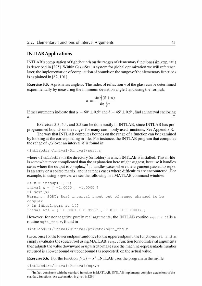
8/6/2019 Moore 1966
http://slidepdf.com/reader/full/moore-1966 52/234
5.2. Elementary Functions of Interval Arguments 41
INTLAB Applications
INTLAB’s computation of tight bounds on the ranges of elementary functions (sin, exp, etc.)
is described in [225]. Within GlobSol, a system for global optimization we will reference
later, the implementation of computation of bounds on the ranges of the elementary functions
is explained in [82, 101].
Exercise 5.5. A prism has angle α. The index of refractionn of the glass can be determined
experimentally by measuring the minimum deviation angle δ and using the formula
n =sin 1
2
(δ+
α)
sin 12α
.
If measurements indicate that α = 60◦±0.5◦ and δ = 45◦±0.5◦, find an interval enclosing
n.
Exercises 5.3, 5.4, and 5.5 can be done easily in INTLAB, since INTLAB has pre-
programmed bounds on the ranges for many commonly used functions. See Appendix E.The way that INTLAB computes bounds on the range of a function can be examined
by looking at the corresponding m-file. For instance, the INTLAB program that computesthe range of
√ x over an interval X is found in
<intlabdir>/intval/@intval/sqrt.m
where <intlabdir> is the directory (or folder) in which INTLAB is installed. This m-fileis somewhat more complicated than the explanation here might suggest, because it handlescases where the output is complex,17 it handles cases where the argument passed to sqrt
is an array or a sparse matrix, and it catches cases where difficulties are encountered. Forexample, in using sqrt.m, we see the following in a MATLAB command window:
>> x = infsup(-1,-1)
intval x = [ -1.0000 , -1.0000 ]
>> sqrt(x)
Warning: SQRT: Real interval input out of range changed to be
complex> In intval.sqrt at 140
intval ans = [ -0.0001 + 0.9999i , 0.0001 + 1.0001i ]
However, for nonnegative purely real arguments, the INTLAB routine sqrt.m calls aroutine sqrt_rnd.m, found in
<intlabdir>/intval/@intval/private/sqrt_rnd.m
twice, once for the lower endpoint andonce for the upperendpoint; the function sqrt_rnd.m
simply evaluates the square root using MATLAB’s sqrt function for noninterval arguments
then adjusts the value downward or upward to make sure the machine-representable number
returned is a lower bound or upper bound (as requested) on the actual value.
Exercise 5.6. For the function f(x) = x2, INTLAB uses the program in the m-file
<intlabdir>/intval/@intval/sqr.m
17In fact, consistent with the standard functions in MATLAB, INTLAB implements complex extensions of the
standard functions. An explanation is given in [29].

8/6/2019 Moore 1966
http://slidepdf.com/reader/full/moore-1966 53/234
42 Chapter 5. Introduction to Interval Functions
Print out this file and annotate it, identifying where the lower and upper bounds on X2 are
computed.
Looking back, we see that equations (5.6)–(5.11) define interval-valued functions of
interval variables. We stress that evaluation of one of these functions F , as indicated, at
a given interval X, yields precisely the set f (X) described by equation (5.1). The serious
issue of interval dependency is lurking, however, as we are about to see.
5.3 Interval-Valued Extensions of Real Functions
In the last section, we were able to define a few interval-valued functions. We did this by
selecting a real-valued function f and computing the range of values f (x) taken as x varied
through some interval X. By definition, the result was equal to the set image f (X).
Here we will consider a different process: that of extending a given real-valued
function f by applying its formula directly to interval arguments.
Formulas and Interval Extensions
Let us begin with an example. Consider the real-valued function f given by
f (x) = 1 − x, x ∈ R. (5.12)
Note carefully that a function is defined by two things: (1) a domain over which it acts, and
(2) a rule that specifies how elements of that domain are mapped under the function. Both
of these are specified in (5.12): the elements of Dom f are real numbers x, and the mapping
rule is x → 1 − x. Taken in isolation, the entity
f (x) = 1 − x (5.13)
is a formula—not a function. Often this distinction is ignored; in many elementary math
books, for example, we would interpret (5.13) as a function whose domain should be taken
as the largest possible set over which the formula makes sense (in this case, all of R).
However, we will understand that Dom f is just as essential to the definition of f as is the
formula f (x).
Now suppose we take the formula (5.13) that describes function (5.12) and apply it
to interval arguments. The resulting interval-valued function
F(X) = 1 − X, X =
X, X
, (5.14)
is an extension of the function (5.12): we have enlarged the domain to include nondegenerate
intervals X as well as the degenerate intervals x = [x, x].
Definition 5.2. We say that F is an interval extension of f , if for degenerate interval
arguments, F agrees with f :F ([x, x]) = f (x). (5.15)
Let us compare F(X) with the set image f (X). We have, according to the laws of
interval arithmetic,
F(X) = [1, 1] −
X, X
= [1, 1] +
−X, −X
=
1 − X, 1 − X
.
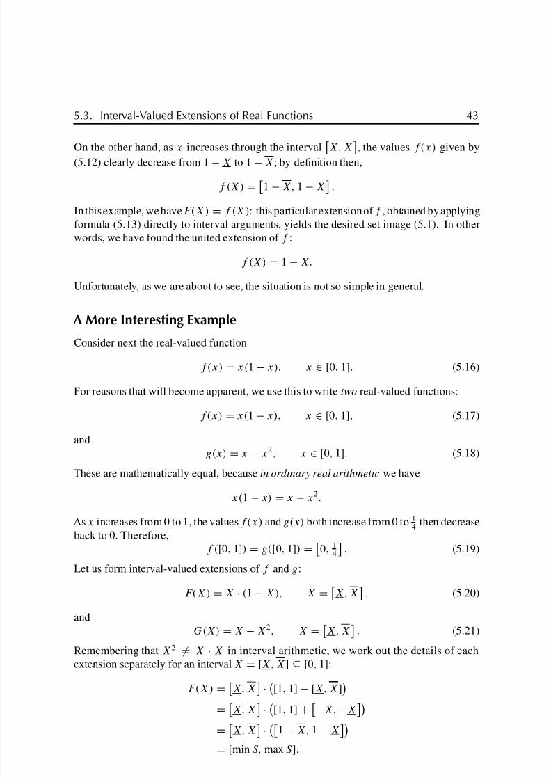
8/6/2019 Moore 1966
http://slidepdf.com/reader/full/moore-1966 54/234
5.3. Interval-Valued Extensions of Real Functions 43
On the other hand, as x increases through the interval
X, X
, the values f(x) given by
(5.12) clearly decrease from 1 − X to 1 − X; by definition then,
f (X) =
1 − X, 1 − X
.
In this example, we have F(X) = f (X): this particular extension of f , obtained by applying
formula (5.13) directly to interval arguments, yields the desired set image (5.1). In other
words, we have found the united extension of f :
f (X) = 1 − X.
Unfortunately, as we are about to see, the situation is not so simple in general.
A More Interesting Example
Consider next the real-valued function
f(x) = x(1 − x), x ∈ [0, 1]. (5.16)
For reasons that will become apparent, we use this to write two real-valued functions:
f(x) = x(1 − x), x ∈ [0, 1], (5.17)
and
g(x) = x − x2, x ∈ [0, 1]. (5.18)
These are mathematically equal, because in ordinary real arithmetic we have
x(1 − x) = x − x2.
As x increases from 0 to 1, the values f(x) and g(x) both increase from 0 to 14
then decrease
back to 0. Therefore,
f ([0, 1]) = g([0, 1]) =
0, 14
. (5.19)
Let us form interval-valued extensions of f and g:
F(X) = X · (1 − X), X =
X, X
, (5.20)
and
G(X) = X − X2, X =
X, X
. (5.21)
Remembering that X2 = X · X in interval arithmetic, we work out the details of each
extension separately for an interval X = [X, X] ⊆ [0, 1]:
F(X) =
X, X
·
[1, 1] − [X, X]
=
X, X
·
[1, 1] +
−X, −X
=
X, X
·
1 − X, 1 − X
= [min S, max S ],

8/6/2019 Moore 1966
http://slidepdf.com/reader/full/moore-1966 55/234
44 Chapter 5. Introduction to Interval Functions
where
S = { X(1 − X), X(1 − X), X(1 − X), X(1 − X)},
while
G(X) =
X, X
−
X, X2
=
X, X
−
X2, X
2
=
X, X
+
−X2
, −X2
=
X − X2
, X − X2
.
Putting, say, X = [0, 1], we see that G(X) = F(X); the two formulas involved in (5.17)
and (5.18)—again, identical in ordinary arithmetic—give rise to different extensions, and
neither of these maps the interval [0, 1] into the interval
0, 14
. We have F ([0, 1]) = [0, 1]
and G([0, 1]) = [−1, 1].
We stress that two expressions can be equivalent in real arithmetic but not equivalent
in interval arithmetic. This is due to the lack of distributivity and additive and multiplicative
inverses in interval arithmetic.
It turns out that the united extension of the original function f arises from use of a
third equivalent formula:h(x) = 1
4−
x − 12
2.
We get
H(X) = 14
−
X − 12
2
=
14
, 14
−
X, X
−
12
, 12
2
=
14
, 14
−
X − 12
, X − 12
2
=
14
, 14
−
(X − 1
2)2, (X − 1
2)2 , X ≥ 1
2,
(X − 1
2)2, (X − 1
2)2
, X ≤ 12
,
0, max{(X − 12
)2, (X − 12
)2}
, X < 12
< X,
so that
H(X) =
14
− (X − 12
)2, 14
− (X − 12
)2
, X ≥ 12
,14
− (X − 12
)2, 14
− (X − 12
)2
, X ≤ 12
,14
− max{(X − 12
)2, (X − 12
)2}, 14
, X < 1
2< X.
It is easily verified that this is f(X). We have H ([0, 1]) = 0, 1
4.
Exercise5.7. Let A1 = [0, 1], A2 = [1, 2],and A3 = [−2, 1]. Evaluate the two expressions
(A1 − A2) · (A3/A2) and (A1/A2 − 1) · A3
and compare the results. Note that these expressions would be equivalent in ordinary
arithmetic.
8/6/2019 Moore 1966
http://slidepdf.com/reader/full/moore-1966 56/234
5.4. The Fundamental Theorem and Its Applications 45
Exercise 5.8. Show that there is never a unique interval extension of a given real
function.
Exercise 5.9. Evaluation of (x − 1)6 for values near x = 1 is sometimes used in traditional
numerical analysis courses to illustrate the effects of roundoff error. In particular, if we
define
f(x) = x6 − 6x5 + 15x4 − 20x3 + 15x2 − 6x + 1,
g(x) = 1 + x(−6 + x(15 + x(−20 + x(15 + x(−6 + x))))),
h(x) = (x − 1)6,
then f , g, and h define the same real-valued function. However, if one evaluates f , g, and
h using floating point arithmetic at points near x = 1 and plots the results, one obtains very
different graphs. A related phenomenon occurs with interval values.
1. Use floating point evaluation within MATLAB to make approximate plots of f , g,
and h at 100 points in [0.999, 1.001].
2. Using INTLAB, set X = infsup(0.999,1.001) and evaluate f,g,h over X.
3. Compare parts 1 and 2. Observe the effects of roundoff error in the floating point
plots of f , g, and h. Which expression is most prone to roundoff “noise”? Does the
susceptibility to roundoff noise correlate with the width of the corresponding interval
extension?
5.4 The Fundamental Theorem and Its Applications
Subset Property of United Extension
Looking back at (5.3), we see that the united extension g has the following subset property:
X,Y ∈ S(M 1) with X ⊆ Y =⇒ g(X) ⊆ g(Y). (5.22)
We will return to this observation momentarily.
Interval Extensions of Multivariable Functions
So far, we have limited ourselves to functions of a single interval variable X. In principle,
there is no reason we should avoid more general functions,
f = f (X1, . . . , Xn),
depending on n interval variables X1, . . . , Xn.
Definition 5.3. By an interval extension of f , we mean an interval-valued function F of ninterval variables X1, . . . , Xn such that for real arguments x1, . . . , xn we have
F(x1, . . . , xn) = f (x1, . . . , xn). (5.23)
That is, if the arguments of F are degenerate intervals, then the left-hand side of (5.23) is
a degenerate interval equal to the right-hand side.

8/6/2019 Moore 1966
http://slidepdf.com/reader/full/moore-1966 57/234
46 Chapter 5. Introduction to Interval Functions
As simple yet crucial examples of two-variable functions, we have the operations
of interval arithmetic. Let us take interval addition as an example. Although we do not
normally do so, we could denote this binary operation as a function of two variables:
f (X1, X2) = X1 + X2 = {x1 + x2 : x1 ∈ X1, x2 ∈ X2}.
The notation is consistent with our previous usage: indeed, it follows from the set definition
on the right that interval addition is the united extension of the function
f (x1, x2) = x1 + x2
that describes ordinary numerical addition. The operations of interval arithmetic are all
defined in this way—recall (4.1). The essential observation is that the interval arithmetic
functions are united extensions of the corresponding real arithmetic functions.
Inclusion Isotonicity
Definition 5.4. We say that F = F (X1, . . . , Xn) is inclusion isotonic if
Y i ⊆ Xi for i = 1, . . . , n =⇒ F (Y 1, . . . , Y n) ⊆ F (X1, . . . , Xn).
Observe carefully that united extensions, which all have the subset property, areinclusion isotonic. In particular, then, the operations of interval arithmetic must satisfy
Y 1 ⊆ X1, Y 2 ⊆ X2 =⇒ Y 1 Y 2 ⊆ X1 X2. (5.24)
We made this observation in section 4.3. Here, we will go a step further.
Rational Interval Functions
Definition 5.5. A rational interval function is an interval-valued function whose values are
defined by a specific finite sequence of interval arithmetic operations.
Example 5.1. Consider the function given by
F (X1, X2) = ([1, 2]X1 + [0, 1]) X2.
The computation of F (X1, X2) can be broken down into the finite sequence of interval
arithmetic operations described by
T 1 = [1, 2]X1 (one interval multiplication),
T 2 = T 1 + [0, 1] (one interval addition),
F (X1, X2) = T 2X2 (one interval multiplication).
Hence F is a rational interval function.
By nature, a rational interval function must arise as an extension of some real-valued
function. In the example above, F (X1, X2) extends a real function of the form
f (x1, x2) = (c1x1 + c2)x2,

8/6/2019 Moore 1966
http://slidepdf.com/reader/full/moore-1966 58/234
5.4. The Fundamental Theorem and Its Applications 47
where c1 and c2 are constants. The function
F(X) = m(X)+ 12(X −m(X))
is not a rational interval function (even though its computation entails only a finite number
of operations) because m(X) = (X +X)/2 is not an interval arithmetic operation.
Lemma 5.1. All rational interval functions are inclusion isotonic.
Proof. The lemma follows by finite induction from (5.24) and the transitivity of the relation
⊆.
The Fundamental Theorem
We are now ready to state a central theorem.
Theorem 5.1 (Fundamental Theorem of Interval Analysis [148]). If F is an inclusion
isotonic interval extension of f , then
f (X1, . . . , Xn) ⊆ F(X1, . . . , Xn).
Proof. By definition of an interval extension, f (x1, . . . , xn) = F(x1, . . . , xn). If F is
inclusion isotonic, then the value of f is contained in the interval F(X1, . . . , Xn) for every
(x1, . . . , xn) in (X1, . . . , Xn).
Natural Interval Extensions
In section 5.3, we obtained extensions F of real rational functions f by replacing (1) the
real variable x with an interval variable X and (2) the real arithmetic operations with corre-
sponding interval operations. The result F is called a natural interval extension of f . The
same procedure can be performed with functions of n variables, and our general observationfrom section 5.3 bears repeating:
Two rational expressions which are equivalent in real arithmetic may not be
equivalent in interval arithmetic.
However, since rational interval functions are inclusion isotonic, we have the following
corollary to Theorem 5.1.
Corollary 5.1. If F is a rational interval function and an interval extension of f , then
f (X1, . . . , Xn)⊆
F(X1, . . . , Xn).
That is, an interval value of F contains the range of values of the corresponding real function
f when the real arguments of f lie in the intervals shown.
Therefore, we have a means for the finite evaluation of upper and lower bounds on
the ranges of values of real rational functions.

8/6/2019 Moore 1966
http://slidepdf.com/reader/full/moore-1966 59/234
48 Chapter 5. Introduction to Interval Functions
Example 5.2. Consider the polynomial
p(x) = 1 − 5x + 13x3. (5.25)
Suppose we wish to know the range of values of p(x) when 2 ≤ x ≤ 3. Since the interval
polynomial
P(X) = 1 − 5X + 13X ·X ·X (5.26)
is a natural interval extension of p(x), the actual range of p(x) values is contained in the
interval
P ([2, 3
])=
1−
5[2, 3
] +1
3 [8, 27
] = −34
3
, 0 .A different extension can be obtained by first rewriting p(x) as
q(x) = 1 − x(5 − x2/3).
A natural interval extension of this is
Q(X) = 1 −X(5 −X · X/3), (5.27)
and a straightforward calculation yields
Q(
[2, 3
])
= [−10,
−3
].
This narrower interval provides a better estimate for the desired range of values of
p(x).
Using ordinary calculus, it is easy to verify that the exact range of values for p(x) in
the preceding example is
p(x) ∈− 10
3
√ 5 + 1 , −5
= [−6.453559 . . . ,−5] for x ∈ [2, 3]. (5.28)
Exercise 5.10. Verify (5.28).
However, an important point is that we can find intervals containing the exact rangeof values without calculus — just by a single evaluation of an interval expression.
We cannot find (5.28) exactly by any finite sequence of arithmetic operations with
rational numbers, since√
5 is irrational. In Chapter 6, we will discuss interval methods for
computing convergent sequences of upper and lower bounds to exact ranges of values.
At this time, we point out that for polynomials, the nested form
A0 +X(A1 +X(A2 + · · · +X(An) · · · )usually gives better (and never gives worse) results than the sum-of-powers form
A0 +
A1X+A
2X·X+ · · · +
AnX·X· · · · ·
X.
This statement holds by (4.4).
It turns out that any natural interval extension of a rational function in which each
variable occurs only once (if at all) and to the first power only will compute the exact range
of values provided that no division by an interval containing zero occurs. Equation (5.14)
was a simple example of such an extension. A proof will be provided in Chapter 6.
8/6/2019 Moore 1966
http://slidepdf.com/reader/full/moore-1966 60/234
5.5. Remarks on Numerical Computation 49
Exercise 5.11. Show by a counterexample that the interval function
F(X) = m(X) + 12
(X − m(X))
is not inclusion isotonic.
Exercise 5.12. The resistance of a parallel combination of two electrical resistors is given
by the formula R−1 = R−11 + R−1
2 . If R1 and R2 have nominal values of 47 and 10 ,
respectively, and manufacturing tolerances of 10%, find an interval enclosure for R. Repeat
using the formula R = (R1R2)/(R1 + R2), which is equivalent in real arithmetic.
Exercise 5.13. Find f ([0, 3]) if f(x) = 13
x3 − 2x. Compare with enclosures found by
evaluating some interval extensions of f .
A Further Property of Natural Extensions
Suppose that F(X) is a natural interval extension of a real rational function f(x), and
suppose we can evaluate F (X0) for some interval X0 without encountering a division by
an interval containing zero. Then the range of values of f(x) for x in X0 is bounded by
F (X0) ≤ f(x) ≤ F (X0).
Hence, f(x) cannot have any poles in X0. Furthermore, by the inclusion isotonicity of the
interval arithmetic operations (and hence of F(X)), no division by an interval containing
zero will occur during the evaluation of the same expression for F(X) for any X ⊆ X0. In
other words, if F (X0) is defined, then F(X) also is for every X ⊆ X0.
5.5 Remarks on Numerical Computation
As we close this chapter, let us remember that interval methods are for use with computers.
In particular, IAis an integral part of these methods. A principal goal of interval computationis to use computers to produce pairs of numbers, between which there are exact solutions
of various kinds of computational problems.
In section 5.2 we defined X2, where X is an interval. Higher integral powers Xn are
defined by
Xn =
Xn, X
n
if X > 0 or n is odd,X
n, Xn
if X < 0 and n is even,
[0, |X|n] if 0 ∈ X and n is even.
(5.29)
This way we have Xn = {xn : x ∈ X}
for each n. To take the limited precision of machine arithmetic into account, we can treat X,
X, and |X| as degenerate intervals and compute Xn, Xn
, and |X| in IA, using the appropriate
endpoint obtained in this way in (5.29). Thus we can compute, in each case, a machine
interval containing the exact result.

8/6/2019 Moore 1966
http://slidepdf.com/reader/full/moore-1966 61/234
50 Chapter 5. Introduction to Interval Functions
Exercise 5.14. Study the INTLAB file
<intlabdir>/intval/@intval/power.m
Explain where (5.29) is implemented. What other necessary complication exists in this
function?
In section 5.2 we used monotonicity to calculate the images of intervals X under
certain common functions. We saw examples of the fact that if f is increasing, then
f (X) =
f (X), f (X)
,
while if f is decreasing, then
f (X) =
f (X), f (X)
.
These united extension values are, of course, inaccessible in practice because the required
endpoints cannot be computed exactly. However, we can extend the machine-computed
endpoints outward in each case by an amount just great enough to include the approximation
error for each such function. This is done automatically by interval software packages such
as INTLAB. In this way we can compute, on the machine, intervals containing the exact
ranges of values. The resulting functions are inclusion isotonic.Using similar approaches, we can construct inclusion isotonic interval extensions of
all functions commonly used in computing.
In the next chapter, we introduce theory and practice for computing refinements of
interval extensions, such that we enclose the corresponding united extensions arbitrarily
closely.

8/6/2019 Moore 1966
http://slidepdf.com/reader/full/moore-1966 62/234
Chapter 6
Sequences of Intervals andInterval Functions
6.1 A Metric for the Set of Intervals
Review of Convergence and Continuity
In real analysis, we call a sequence {xk} convergent if there exists a real number x∗
suchthat for every ε > 0 there is a natural number N = N(ε) such that
|xk − x∗| < ε (6.1)
whenever k > N . In this case, we write
x∗ = limk→∞
xk or xk → x∗
and refer to x∗ as the limit of {xk}. The quantity |xk−x∗| in (6.1) is just the distance between
xk and x∗ as measured along the real line.
The notion of sequence convergence appears throughout mathematics. One can con-
sider convergent sequences of complex numbers, real-valued functions of a real variable,etc. All that is needed is a suitable measure of “distance” between the objects of interest.
Let us also recall the definition of ordinary function continuity. We say that f(x) is
continuous at a point x0 if for every ε > 0 there is a positive number δ = δ(ε) such that
|f(x) − f (x0)| < ε (6.2)
whenever |x − x0| < δ. In this case, |f(x) − f (x0)| is the distance between the y-axis
points f(x) and f (x0), corresponding to the distance |x − x0| along the x-axis.
It is said that convergence and continuity are the two central concepts of analysis. We
see, in turn, how they both hinge on having a suitable way to express distance. The need to
discuss convergence and continuity outside of ordinary real analysis has led to a powerful
generalization of the distance idea.
Notion of Metric
Let S be any set, and suppose that a real-valued function d is defined such that for any two
elements x, y ∈ S the following statements hold:
51

8/6/2019 Moore 1966
http://slidepdf.com/reader/full/moore-1966 63/234

8/6/2019 Moore 1966
http://slidepdf.com/reader/full/moore-1966 64/234
6.2. Refinement 53
Exercise 6.4. Show that (6.3) has the following additionalproperties: (a)d(X+Z, Y +Z) =
d(X,Y); (b) d(X,Y) ≤ w(Y) when X ⊆ Y ; (c) d(X, 0) = |X|.
Exercise 6.5. In INTLAB, (6.3) is implemented with the function qdist(X,Y):
>> X = infsup(-1,1);
>> Y = infsup(1/2,5/2);
>> qdist(X,Y)
ans = 1.5000
Similarly, the width of an interval X is implemented with the function diam(X). (For a listof these and other INTLAB functions, see Appendix E. Help for a specific function listed
there can be obtained in the command window with the “help” command. For example,
issuing help diam gives a summary of how to use the INTLAB diam function.18) Illustrate
Exercise 6.4 by using the INTLAB functions qdist and diam.
6.2 Refinement
According to the fundamental theorem of interval analysis, we have
f (X1, . . . , Xn) ⊆ F(X1, . . . , Xn) (6.4)
for any inclusion isotonic interval extension F of a real function f . This means that an
interval value of F contains the range of values of the corresponding real function f when
the real arguments of f lie in the intervals X1, . . . , Xn. In Chapter 5, we saw an example in
which equality held in (6.4), but we also saw examples in which the width of the right-hand
side substantially exceeded that of the left-hand side.
Lipschitz Interval ExtensionsWe now examine a process by which f (X1, . . . , Xn) may be approximated as closely as
desired by a finite union of intervals. We begin with a concept closely related to continuity.
Definition 6.1. An interval extension F is said to be Lipschitz in X0 if there is a constant L
such that w(F(X)) ≤ Lw(X) for every X ⊆ X0.
Hence, the width of F(X) approaches zero at least linearly with the width of X. Here
X may be an interval or an interval vector X = (X1, . . . , Xn).
Lemma 6.1.If F is a natural interval extension of a real rational function with F(X)
defined for X ⊆ X0, where X and X0 are intervals or n-dimensional interval vectors, then
F is Lipschitz in X0.
18Issuing the help command for a particular function will also list, in blue, different versions of the function,
for different data types. Clicking on one of these links gives information about the function when used with that
data type.

8/6/2019 Moore 1966
http://slidepdf.com/reader/full/moore-1966 65/234
54 Chapter 6. Interval Sequences
Proof. For any real numbers a and b and any intervals Xi and Y i , we have the following
relations (which are not hard to prove):
w(aXi + bY i ) = |a|w(Xi ) + |b|w(Y i ),
w(Xi Y i ) ≤ |Xi |w(Y i ) + |Y i |w(Xi ),
w(1/Y i ) ≤ |1/Y i |2w(Y i ) if 0 /∈ Y i . (6.5)
Since the natural interval extension has interval values F(X) obtained by a fixed finite
sequence of interval arithmetic operations on real constants (from a given finite set of
coefficients) and on the components of X (if X is an interval vector) and since X ⊆ X0
implies that |Xi | ≤ X0 for every component of X, it follows that a finite number of
applications of (6.5) will produce a constant L such that w(F(X)) ≤ Lw(X) for all X ⊆
X0.
By the following result, certain interval extensions of irrational functions are also
Lipschitz.
Lemma 6.2. If a real-valued function f(x) satisfies an ordinary Lipschitz condition in X0,
|f(x) − f(y)| ≤ L|x − y| for x, y ∈ X0,
then the united extension of f is a Lipschitz interval extension in X0.
Proof. The function f is necessarily continuous. The interval (or interval vector) X0 is
compact. Thus, w(f (X)) = |f (x1) − f (x2)| for some x1, x2 ∈ X ⊆ X0. But |x1 − x2| ≤
w(X); therefore, w(f (X)) ≤ Lw(X) for X ⊆ X0.
It follows that interval extensions which are united extensions, such as the following,
are also Lipschitz in X0:
1. Xn given by (5.29);
2. eX
= [eX
, eX
];
3. X1/2 = [X1/2 , X1/2
] for 0 < X0;
4. ln X =
ln X , ln X
for 0 < X0;
5. sin X =
sin X , sin X
for X0 ⊆
− π2
, π2
;
6. sin X = [minx∈X(sin x) , maxx∈X(sin x)] for arbitrary X0.
Lemma 6.3. Let F and G be inclusion isotonic interval extensions with F Lipschitz in Y 0,
G Lipschitz in X0, and G(X0) ⊆ Y 0. Then the composition H(X) = F (G(X)) is Lipschitz
in X0 and is inclusion isotonic.
Proof. The inequality
w(H(X)) = w(F (G(X)) ≤ L2w(G(X)) ≤ L2L1w(X)
shows that H is Lipschitz in X0.
8/6/2019 Moore 1966
http://slidepdf.com/reader/full/moore-1966 66/234

8/6/2019 Moore 1966
http://slidepdf.com/reader/full/moore-1966 67/234
56 Chapter 6. Interval Sequences
Proof. Relation (6.9) follows from the fact that f(X) = ∪s f (Xs ), where the Xs are the
elements of the uniform subdivision. We have F (Xs ) = f (Xs ) + Es for some Es and
w(Es ) = w(F(Xs )) − w(f (Xs )) ≤ w(F(Xs )) ≤ Lw(Xs ) ≤ Lw(X)/N
for each Xs . The inequality for w(EN ) holds with K = 2L since, in the worst case,
the maximum excess width may have to be added to both upper and lower bounds in the
union.
We can compute arbitrarily sharp lower and upper bounds on the exact range of values
of a wide variety of real-valued functions of n variables by subdividing the domain of arguments and taking the union of interval evaluations over the elements of the subdivision.
This technique, also known as splitting, converges at least linearly in the width of the pieces
in the subdivision.
Example 6.3. Consider the function f(x) = x − x2 for x ∈ [0, 1]. It is easily verified that
f ([0, 1]) =
0, 14
. The interval extension
F(X) = X − X · X
has F ([0, 1]) = [−1, 1]. Hence, its excess width is 2 − 14
= 74
. Let us split [0, 1] into n
subintervals Xi = [(i − 1)/n,i/n], 1 ≤ i ≤ n. We now compute the range of values of F(X) over each of these subintervals and then take the union of the resulting intervals to
find a narrower interval still containing the range of values of F(X). The table below gives
numerical results for a few values of n:
n F (n)(X)
1 [−1, 1]
2 [−0.5, 0.75]
10 [−0.1, 0.35]
100 [−0.01, 0.26]
1000 [−0.001, 0.251]10000 [−0.0001, 0.2501]
These strongly suggest convergence, and every F (n)(X) contains the exact range of values0, 1
4
.
Exercise 6.6. The computations in Example 6.3 can be done neatly in MATLAB using theINTLAB toolbox. In particular, F(X) can be programmed:
function Y = example6p3(X)
Y = X - X * X ;
(The above MATLAB code should be put into a file named example6p3.m. This happensautomatically if MATLAB’s editor is used and the default “save file” is done the first timethe file is saved.) Computation of a row of the table in Example 6.3 can be done with thefollowing function:
function Y = refinement(X,f,N)
% Y = refinement(X,f,N)

8/6/2019 Moore 1966
http://slidepdf.com/reader/full/moore-1966 68/234
6.3. Finite Convergence and Stopping Criteria 57
% computes a uniform refinement of the interval X with N
% subintervals, to compute an interval enclosure for
% the range of the interval function f (passed as a
% character string). See Section 6.2 of "Introduction
% to Interval Analysis" by Moore, Kearfott, and Cloud.
% First form the N subintervals --
h = (sup(X)-inf(X))/N;
xi=inf(X);
x1=xi;
for i=1:N% This is more accurate for large N than
% x i p 1 = x i + h
xip1 = x1 + i*h;
Xs(i) =infsup(xi,xip1);
% Do it this way so there are no "cracks" due
% to roundoff error --
xi=xip1;
end
% Redefine the upper bound to eliminate roundoff
% error problems --
Xs(N) = infsup(inf(Xs(N)),sup(X));
% Now compute the extension by computing the natural
% extensions over the subintervals and taking the union --
Y = feval(f,Xs(1));
if N>1
for i=2:N
Y = hull(Y,feval(f,Xs(i)));
end
end
For example, we might create the following dialogue in the MATLAB command window:
>> X = infsup(0,1);>> Y = refinement(X,’example6p3’,10)
intval Y = [ -0.1000 , 0.3501 ]
Use this to check the table in Example 6.3.
6.3 Finite Convergence and Stopping Criteria
Nested Interval Sequences
Definition 6.5. An interval sequence {Xk} is nested if Xk+1 ⊆ Xk for all k.
Lemma 6.4. Every nested sequence {Xk} converges and has the limit∩∞k=1Xk.
Proof. {Xk} is a nondecreasing sequence of real numbers, bounded above by X1, and so
has a limit X. Similarly, {Xk} is nonincreasing and bounded below by X1 and so has a
limit X. Furthermore, since Xk ≤ Xk for all k, we have X ≤ X. Thus {Xk} converges to
X =X,X
= ∩∞
k=1Xk.

8/6/2019 Moore 1966
http://slidepdf.com/reader/full/moore-1966 69/234
58 Chapter 6. Interval Sequences
Lemma 6.5. Suppose {Xk} is such that there is a real number x ∈ Xk for all k. Define {Y k}
by Y 1 = X1 and Y k+1 = Xk+1 ∩ Y k for k = 1, 2, . . .. Then Y k is nested with limit Y , and
x ∈ Y ⊆ Y k for all k. (6.10)
Proof. By induction, the intersection defining Y k+1 is nonempty so {Y k} is well defined. It
is nested by construction. Relation (6.10) follows from Lemma 6.4.
Finite Convergence
Definition 6.6. By the finite convergence of a sequence {Xk }, we mean there is a positive
integer K such that Xk = XK for k ≥ K. Such a sequence converges in K steps.
Example 6.4. It is not hard to see that
X0 = [1, 2], Xk+1 = 1 + Xk/3 (k = 0, 1, 2, . . . ) ,
generates a nested sequence {Xk}. The rational interval function F(X) = 1 + X/3 is
inclusion isotonic. Therefore, X1 = F (X0) = 1 + [1, 2]/3 =
43
, 53
⊆ X0 = [1, 2]. It
follows that Xk+1 = F (Xk) ⊆ Xk for all k by finite induction. By Lemma 6.4, the sequence
has a limit X. If we compute {Xk} using IA, we will obtain a sequence {X∗
k
} with Xk ⊆ X∗
kfor all k. More precisely, let X∗k be defined by X∗
0 = X0 = [1, 2], and
X∗k+1 = {1 + X∗
k /3 : computed in IA} ∩ X∗k
for k = 0, 1, 2, . . . (which we can apply, since X ⊆ Xk for all k). It follows from Lemma 6.5
that X∗k is nested and that the limit of {Xk} is contained in the limit X∗ of {X∗
k }. The sequence
{X∗k } will converge in a finite number of steps. For instance, with three-digit IA we find
X∗0 = [1, 2],
X∗1 = [1.33, 1.67],
X∗2 = [1.44, 1.56],
X∗3 = [1.48, 1.52],
X∗4 = [1.49, 1.51],
X∗5 = [1.49, 1.51],
and X∗k = X∗ for all k ≥ 4. We have finite convergence in four steps. The real sequence
xk+1 = 1 + xk/3 converges to 1.50 (after infinitely many steps) from any x0.
We can also illustrate the finite convergence of the sequence in Example 6.4, as well asillustrate use of the uncertainty representation within INTLAB, with the following INTLAB
function:
function [X] = finite_convergence_example()
% Implements the computations for the finite convergence
% example in Chapter 6 of Moore / Kearfott / Cloud
format long;
intvalinit(’Display_’);

8/6/2019 Moore 1966
http://slidepdf.com/reader/full/moore-1966 70/234
6.3. Finite Convergence and Stopping Criteria 59
X = infsup(1,2);
X_new = infsup(-Inf,Inf);
i=0;
while (X_new ˜= X)
i=i+1;
X = intersect(X,X_new);
i,X
X_new = 1+ X/3;
end
When finite_convergence_example is issued from the MATLAB command prompt,
the following output (edited for brevity) ensues:
finite_convergence_example
===> Default display of intervals with uncertainty (e.g. 3.14_),
inf/sup or mid/rad if input too wide
i = 1, intval X = [ 1.00000000000000 , 2.00000000000000 ]
i = 2, intval X = [ 1.33333333333333 , 1.66666666666667 ]
i = 3, intval X = [ 1.44444444444444 , 1.55555555555556 ]
i = 4, intval X = 1.5_____________
i = 5, intval X = 1.50____________
i = 6, intval X = 1.50____________
i = 7, intval X = 1.500___________i = 8, intval X = 1.500___________
.
.
.
i = 28, intval X = 1.5000000000000_
i = 29, intval X = 1.5000000000000_
i = 30, intval X = 1.50000000000000
i = 31, intval X = 1.50000000000000
i = 32, intval X = 1.50000000000000
i = 33, intval X = 1.50000000000000
i = 34, intval X = 1.50000000000000diary off
This illustrates that approximately half a decimal point of accuracy is gained on each iteration
and that, indeed, the convergence ends after a finite number of steps (34 steps) when using
standard binary arithmetic.
Next we examine a sequence of refinements computed in IA and intersected to yield
a nested sequence that converges in a finite number of steps.
Example 6.5. Consider the interval polynomial F(X) = X(1 − X) and its refinements
F (N )(X). Let X = [0, 1] and take the sequence
Y 1 = F (1)([0, 1]) = F ([0, 1]), Y k+1 = F (k+1)([0, 1]) ∩ Y k (k = 1, 2, . . . ) .
The intersections are nonempty because each refinement contains the range of values of
f(x) = x(1 − x) for x ∈ [0, 1], namely [0, 14
]. By construction, {Y k} is nested. By
Theorem 6.1 and Lemma 6.5,
f(X) =∞
k=1 F (k)(X) = limk→∞
Y k . (6.11)

8/6/2019 Moore 1966
http://slidepdf.com/reader/full/moore-1966 71/234
60 Chapter 6. Interval Sequences
We have
F (k)([0, 1]) =
0, 1
4+ 1/(2k) + 1/(4k2)
, k odd,
0, 14
+ 1/(2k)
, k even.
We can compute a subsequence of {Y k}, for example, for k of the form k = 2t , t = 1, 2, . . ..
If we compute the nested sequence of intervals Y ∗1 = [0, 1], and for t = 1, 2, . . .,
Y ∗t +1 = F ∗(2t )([0, 1]) ∩ Y ∗i ,
where F ∗(k)([0, 1]) is F (k) ([0, 1]) computed in three-place IA, we obtain again a nested
sequence {Y ∗t }. This converges in nine steps to the interval [0, 0.251]. We have Y ∗t =
[0, 0.251] for all t ≥ 9.
Natural Stopping Criterion
For any fixed (as opposed to “variable”) precision representation of machine numbers,
there is a finite set of machine numbers represented by strings of bits b0b1 . . . bs with s
fixed. Hence there is only a finite set of intervals with machine number endpoints. Any
nested sequence of such intervals is necessarily finitely convergent.
For any iterative interval method that produces a nested sequence with endpoints
represented by fixed precision machine numbers, we have a natural stopping criterion.
Since the sequence {Xk} converges in a finite number of steps, we can compute the Xk until
Xk+1 = Xk. (6.12)
If the Xk are generated by a procedure of the form
Xk+1 = F (Xk) (6.13)
such that each Xk+1 depends only on the previous Xk, then it is clear that (6.12) is sufficient
to guarantee convergence.
In particular, if F(X) is a rational expression in X and if X0 is an interval such that
F (X0) ⊆ X0, which can be tested on the computer, it follows that {Xk } defined by
Xk+1 = F (Xk) (k = 0, 1, 2, . . .) (6.14)
is nested with
X0 ⊇ X1 ⊇ X2 ⊇ · · ·
and hence converges to some X∗ with X∗ = F (X∗) and X∗ ⊆ Xk for all k = 0, 1, 2, . . ..
With IA, it may happen that X1 = F (X0) ⊆ X0 but that Xk+1 Xk for some k. If
instead of (6.14), we compute
Xk+1 = F (Xk) ∩ Xk (6.15)
and stop when (6.12) is satisfied (which will happen always for some k using fixed finite
precision IA), we have the narrowest possible interval containing X∗ = F (X∗). A narrowerinterval would require using higher-precision arithmetic.
Furthermore, if for a chosen X0, the interval F (X0) ∩ X0 is empty, then X0 contains
no fixed points of F (i.e., there is no X ∈ X0 such that F(X) = X). This follows from the
inclusion isotonicity of F , for if F(X) = X and X ⊆ X0, then X = F(X) ⊆ F (X0) and so
X ⊆ F (X0) ∩ X0; therefore, if F (X0) ∩ X0 is empty, there is no such X.

8/6/2019 Moore 1966
http://slidepdf.com/reader/full/moore-1966 72/234
6.3. Finite Convergence and Stopping Criteria 61
Example 6.6. Let
F(X) = 12
X + 2.
If we take X0 = [1, 2], then
F (X0) = 12
[1, 2] + 2 =
52
, 3
.
Since F (X0) ∩ X0 = ∅, there is no fixed point of F in [1, 2]. If we take X0 =
2, 72
instead,
then
F (X0) = 12
2, 7
2
+ 2 =
3, 15
4
.
Here F (X0) ∩ X0 =
3, 72
; we cannot conclude anything since F (X0) X0. Finally, with
X0 = [2, 5], we have F (X0) = F ([2, 5]) =
3, 92
. This time, F (X0) ⊆ X0, so F has a
fixed point X in X0. The iterations
Xk+1 = F (Xk) ∩ Xk, k = 0, 1, 2, . . . , (6.16)
produce, in three-digit IA,
X1 = [3, 4.5] ∩ [2, 5] = [3, 4.5],
X2 = [3.5, 4.25] ∩ [3, 4.5] = [3.5, 4.25],
X3 = [3.75, 4.13] ∩ [3.5, 4.25] = [3.75, 4.13],
X4 = [3.87, 4.07],
X5 = [3.93, 4.04],
X6 = [3.96, 4.02],
X7 = [3.98, 4.01],
X8 = [3.99, 4.01],
X9 = [3.99, 4.01],
Xk+1 = Xk, k = 8, 9, 10, . . . .
F has a fixed point in [3.99, 4.01].
If the process generating the sequence depends explicitly on k as well as on Xk , say,
Xk+1 = F (k, Xk),
then we might have Xk+1 = Xk for some k and yet Xk+2 = Xk even though {Xk } is nested.
An example is
Xk+1 = ([0, 2]/k) ∩ Xk, X1 = [0, 1]. (6.17)

8/6/2019 Moore 1966
http://slidepdf.com/reader/full/moore-1966 73/234
62 Chapter 6. Interval Sequences
Here
X1 = [0, 1],
X2 = [0, 1],
X3 = [0, 1],
X4 = [0, 23
],
X5 = [0, 12
],
...
Xk+1 = [0, 2/k], k > 2.
Hence, (6.12) is a valid stopping criterion if and only if {Xk} is nested and generated by
(6.16) with F (Xk) depending only on Xk.
Remarks on Branching
Let us close this section with some comments about branching in computer programs. For
real numbers x and y, the relation x ≤ y is either true or false. If it is false, then we have
x > y. If all we know about x and y is that they lie in intervals x ∈ X and y ∈ Y , then wecan only deduce one of three possibilities:
(1) If X ≤ Y , then x ≤ y.
(2) If X > Y , then x > y.
(3) Otherwise, we don’t know whether x ≤ y or x > y.
We can modify any computer program by using IA instead of ordinary machine arithmetic
whenever rounding error is possible in an arithmetic operation and by using the above three-
valued logic for all branch tests involving computed quantities which are only known to
lie in certain computed intervals. If we stop the computation whenever a “don’t know”logical value is obtained, then all intervals computed up to that point by the modified
problem contain the exact result of the corresponding finite sequence of operations using
exact (infinite precision) real arithmetic for all arithmetic operations.
Note Although we may, in principle, apply this to all computer programs originally written
with floating point arithmetic, it is unlikely to lead to good results without additional careful
analysis and redesign. For example, if we “don’t know” whether x ≤ y or x > y, we must
take the union of the values of the separate branches, resulting in more computation and
wider intervals. This is often impractical, especially if there are many such branches, and
can lead to unusefully wide enclosures.
Exercise 6.7. The following MATLAB function (which uses INTLAB) performs a singlestep of the iteration (6.15):
function new_X = interval_fixed_point_step(f,X)
% X_star = interval_fixed_point_step(f,X)

8/6/2019 Moore 1966
http://slidepdf.com/reader/full/moore-1966 74/234
6.3. Finite Convergence and Stopping Criteria 63
% returns the result of a step of interval
% fixed point iteration
% X_{k+1} = intersect(X_k, f(X_k)) as explained
% in Section 6.3.
new_X = intersect(X,feval(f,X));
For example, with the function
function Y = example6p4(X)
Y = 1 + X / 3 ;
we can reproduce an analogue of the sequence in Example 6.4, but with correctly outwardlyrounded intervals displayed roughly to machine precision, with the following MATLABdialogue:
>> format long
>> intvalinit(’DisplayInfsup’)
>> X = infsup(1,2)
intval X = [ 1.00000000000000 , 2.00000000000000 ]
>> X = interval_fixed_point_step(’example6p4’,X)
intval X = [ 1.33333333333333 , 1.66666666666667 ]
>> X = interval_fixed_point_step(’example6p4’,X)
intval X = [ 1.44444444444444 , 1.55555555555556 ]
>> X = interval_fixed_point_step(’example6p4’,X)
intval X = [ 1.48148148148148 , 1.51851851851852 ]
>> X = interval_fixed_point_step(’example6p4’,X)
intval X = [ 1.49382716049382 , 1.50617283950618 ]
>> X = interval_fixed_point_step(’example6p4’,X)
intval X = [ 1.49794238683127 , 1.50205761316873 ]
Do the same iteration for Example 6.6.
Exercise 6.8. The MATLAB function from Exercise 6.7 implementing a step of intervalfixed point iteration can be called iteratively to convergence with the following MATLABfunction:
function [X_limit,N] = interval_fixed_point_limit(f,X)
% [X_limit,N] = interval_fixed_point_convergence(f,X) returns
% the limit of fixed point iteration X_{k+1} = f(X_k) as
% explained in Section 6.3, and returns the number of iterations
% required in N. If one or both of the bounds of X_limit is NaN,
% then the limit is the empty set.
old_X = infsup(-Inf,Inf);
N = 0 ;
while (old_X ˜= X) & ˜( isnan(inf(X)) | isnan(sup(X)) )
N = N+1;old_X = X;
X = interval_fixed_point_step(f,X);
end
X_limit = X;
For instance, we might have the following MATLAB dialogue for Example 6.4:

8/6/2019 Moore 1966
http://slidepdf.com/reader/full/moore-1966 75/234
64 Chapter 6. Interval Sequences
>> X = infsup(1,2)
intval X = [ 1.00000000000000 , 2.00000000000000 ]
>> [Y,N] = interval_fixed_point_limit(’example6p4’,X)
intval Y = [ 1.49999999999999 , 1.50000000000001 ]
N = 3 4
(The displayed interval [1.49999999999999, 1.50000000000001] represents an out-
wardly rounded binary-to-decimal conversion of the actual binary representation of the
interval.)
1. Does interval_fixed_point_limit work for Examples 6.5 and 6.6?
2. Can interval_fixed_point_limit fail? If so, how?
3. Do you think an upper bound on the number of iterations allowed in the loop in
interval_fixed_point_limit should be given? If not, then, assuming IEEE
double precision arithmetic, can you compute an upper bound on the number of
iterations actually needed?
6.4 More Efficient Refinements
We have seen that refinement of an interval extension is a method for computing arbitrarily
sharp upper and lower bounds on the range of values of a real function, but it is of prac-
tical importance to be able to obtain these bounds as efficiently as possible. We begin by
characterizing the class of functions most commonly used in computing.
Code Lists and the Class FC
Let FCn(X0) be the class of real-valued functions f of n real variables whose values
f (x1, . . . , xn) for each f are defined for all x = (x1, . . . , xn) in the interval vector X0 =(X10, . . . , Xn0) by some fixed, finite sequence of operations
T 1 = h1(y1, z1)
T 2 = h2(y2, z2)
... (6.18)
f(x) = T M = hM (ym, zm)
for y1, z1 ∈ S 1 = {x1, . . . , xn, c1, . . . , cp}, where c1, . . . , cp are given real numbers (the
coefficients of f ), and where h1, . . . , hM are the arithmetic functions +, −, ·, /, or unary
functions (of only one of the variables yi , zi ) of elementary type: exp(·), ln(·),√ ·, etc.
Furthermore, yi+1, zi+1 ∈ S i+1 = S i ∪ {T i}, i = 1, . . . , M − 1. The integer M , the
coefficients c1, . . . , cp (if any), and the sequence of operations h1, . . . , hM define a particularfunction f ∈ FCn(X0). Each yi , zi may be an x; or a constant ci or one of the previous T j(j < i).
Example 6.7. The function f defined by
f (x1, x2) = x1ex1+x22 − x2
2

8/6/2019 Moore 1966
http://slidepdf.com/reader/full/moore-1966 76/234
6.4. More Efficient Refinements 65
can be expressed as the sequence (commonly called a code list or computational graph)
T 1 = x22 ,
T 2 = x1 + T 1,
T 3 = eT 2,
T 4 = T 3x1,
f (x1, x2) = T 4 − T 1.
Therefore, it belongs to FC2(X0) for any X0.
We assume that we can compute arbitrarily sharp bounds on the exact range of values
of each of the unary functions occurring in the sequence of operations for f(x). The class
FCn is further assumed to include only functions f that are defined for all x ∈ X0 and
that have inclusion isotonic, Lipschitz, interval extensions F(X) for X ⊆ X0. For some of
the discussion to follow, we also assume that the first and second partial derivatives of f
satisfy the same conditions as f . This final assumption, concerning the existence of interval
extensions with desirable properties (inclusion isotonicity, etc.) is satisfied automatically
for all f ∈ FCn(X0), provided only that F(X0) is defined, where F(X) is the interval
extension
T 1 = H 1(Y 1, Z1),
T 2 = H 2(Y 2, Z2),
... (6.19)
F(x) = T M = H M (Y m, Zm),
whereH 1, . . . , H M are the united extensions of the functionsh1, . . . , hM , respectively. This
is the case, replacing real arithmetic operations by interval arithmetic operations and using
the united extensions of the unary functions, as long as for the interval vectorX0, no division
by an interval containing 0 occurs during the computation of T 1, . . . , T M and provided thatno arguments containing zero occur for such unary operations as ln(·) or
√ ·. (The latter
would spoil the Lipschitz property for the interval extension.) Since such an F is inclusion
isotonic, F(X) is defined for every X ⊆ X0.
Under these conditions, Theorem 6.1 states that the excess width of the refinement
F (N)(X) of the interval extension F(X) given by (6.19) of a function f ∈ FCn(X0) satisfies
w(En) ≤ Kf w(X)/N for some Kf depending only on f . (6.20)
An evaluation of F requires one pass through the finite sequence of operations (6.19), just
as an evaluation of f requires one pass through (6.18). An evaluation of F (N)(X), given
by (6.9), requires N n evaluations of F(X). If n is at all large, this involves a prohibitiveamount of computation to achieve the result (6.20) for large N . Even for n = 2 we have,
for N = 1000 (perhaps to reduce the excess width to 0.001), 10002 = 106 evaluations to
carry out.
Fortunately, by using more information about a particular functionf , we can compute
an interval containing the exact range of values and having arbitrarily small excess width

8/6/2019 Moore 1966
http://slidepdf.com/reader/full/moore-1966 77/234
66 Chapter 6. Interval Sequences
with far less work. In some cases, we can even compute an interval with zero excess width
in one evaluation of F(X). In the remainder of this section, we assume that f ∈ FCn(X0)
with F(X) defined for X ⊆ X0 by (6.19).
Theorem 6.2. Ifeachofthevariables x1, . . . , xn occursatmostonceinthelist y1, z1, . . . , yn,
zn of arguments in the sequence (6.18) defining f(x), then the interval extension F(X) de-
fined by (6.19) is the united extension of f for all X ⊆ X0.
Proof. We have F(X) = f(X) if and only if f(X) ⊆ F(X) and F(X) ⊆ f(X). The
first inclusion holds under our assumptions on F(X). Under the further hypothesis of the
theorem, every real number r ∈ F(X) is expressible as r = f(x) for some x = (x1, . . . , xn)with xi ∈ Xi for i = 1, . . . , n. In fact, each H i is the united extension of hi . Therefore
F(X) ⊆ f(X).
Hence, for a function f satisfying the hypotheses of Theorem 6.2, we can compute
the exact range of values of f(x) for x ∈ X ⊆ X0 with one evaluation of F(X) using (6.19).
If some xi occurs more than once in the list of arguments in (6.18), then the corre-
sponding Xi occurs more than once in the list of arguments in (6.19). In this case, there
may be real numbers in F(X) which are not expressible as f(x) for any x ∈ X.
Example 6.8. Consider f ∈ FC1([0, 1]) defined by
T 1 = 1 − x1, f (x1) = T 2 = T 1x1.
The variable x1 occurs twice as an argument. The corresponding list for F(X) is
T 1 = 1 − X1, F (X1) = T 2 = T 1X1.
Now F ([0, 1]) = [0, 1], but there isno x1 ∈ [0, 1] such that f (x1) = (1−x1)x1 = 1 ∈ [0, 1].
On the other hand, the interval function
T 1 = 1 − X1, F (X1, X2) = T 2 = T 1X2,
is the united extension of the real function
T 1 = 1 − x1, f (x1, x2) = T 2 = T 1x2.
In particular, F ([0, 1], [0, 1]) = [0, 1] is the exact range of values of f (x1, x2) = (1 −x1)x2
for x1 ∈ [0, 1] and x2 ∈ [0, 1].
Another explanation for the difference between these two results is the following. In
both cases, we first compute 1 − [0, 1] = [0, 1]. This is the exact range of values of 1 − x1
for x1 ∈ [0, 1]. The discrepancy comes at the next step. When we compute T 1X1 with
T 1 = [0, 1] and X1 = [0, 1], we obtain [0, 1]. We obtain the same result for T 1X2 with
T 1 = [0, 1] and X2 = [0, 1].In the second case, this is the desired exact range of values of f (x1, x2). In the first
case, we get an overestimation of the range of values of f (x1) = (1 − x1)x1 because, during
the numerical evaluation of T 1X1, we have not made use of the information that T 1 = [0, 1]
represents the range of values of 1 − x1 for x1 ∈ X1. We have not distinguished between
this and T 1 = [0, 1] as the range of values of 1 − x2 for a variable x2 independent of x1.
8/6/2019 Moore 1966
http://slidepdf.com/reader/full/moore-1966 78/234
6.4. More Efficient Refinements 67
Example 6.8 shows that it is better to use the interval extension Xn defined by (5.29)
for integer powers xn than to use X ·X ·· · ··X. For X = [−1, 2] we obtainX ·X = [−2, 4],
whereas X2 using (5.29) yields the correct result, [−1, 2]2 = [0, 4] = {x2 : x ∈ [−1, 2]}.
Exercise 6.9. Find the range of values of
g(x,y,z,u,v,w) = (33 − 2x + yz)/(10 − uvw)
over the unit 6-cube x,y,z,u,v,w ∈ [0, 1].
Sometimes we can reduce the number of occurrences of a variable in a real rational
expression by algebraic manipulation.Example 6.9. Let f (x1, x2, x3) be defined by
f (x1, x2, x3) =x1 + x2
x1 − x2
x3, (6.21)
which we can rewrite as
f (x1, x2, x3) = x3
1 +
2
(x1/x2) − 1
. (6.22)
For x1 ∈ [1, 2], x2 ∈ [5, 10], and x3 ∈ [2, 3], the natural interval extension of (6.22)
produces the correct range of values
−7,−
22
9
since each variable occurs only once. How-ever, the natural interval extension of (6.21) produces
−12,− 12
9
with an excess width
of 559
.
Given a function f ∈ FCn(X0) defined by a finite sequence of the form (6.18), we
can construct interval extensions of f other than the natural extension given by (6.19). We
will discuss four: the centered form, the mean value form, a variant of the mean value form
we call the slope form, and the monotonicity-test form.
The Centered Form
We now discuss the centered form, a second-order interval extension. To obtain the centered
form F c(X1, . . . , Xn), we first rewrite f (x1, . . . , xn) as
f (x1, . . . , xn) = f (c1, . . . , cn) + g(y1, . . . , yn) (6.23)
with yi = xi − ci and with g defined by (6.23):
g(y1, . . . , yn) = f (y1 + c1, . . . , yn + cn) − f (c1, . . . , cn).
For rational f , we can express g in the form
g(y1, . . . , yn) = y1h1(y1, . . . , yn) + · · · + ynhn(y1, . . . , yn),
where hi is rational and hi(0, . . . , 0) is defined if f (c1, . . . , cn) is. We define F c by
F c(X1, . . . , Xn) = f (c1, . . . , cn) +
ni=1
Y iH i(Y 1, . . . , Y n), (6.24)
where ci = m(Xi), Y i = Xi − ci , and H i is the natural interval extension of hi .

8/6/2019 Moore 1966
http://slidepdf.com/reader/full/moore-1966 79/234
68 Chapter 6. Interval Sequences
Example 6.10. We reconsider the polynomial p(x) = 1 − 5x + 13
x3 given in (5.25). We
rewrite p(x) as
p(x) = 1 − 5c + 13
c3 + g(y), where y = x − c,
and
g(y) = p(x) − p(c) = y(−5 + 13
((y + c)2 + (y + c)c + c2)).
We define P c by
P c(X) = p(c) + YH(Y),
where c = m(X), Y = X − m(X), and
H( Y ) = −5 + 13
((Y + c)2 + (Y + c)c + c2).
Now, for X = [2, 3], we obtain
c = m(X) = 52
, Y =− 1
2, 1
2
, p(c) = p( 5
2) = − 151
24.
We have H( Y ) =
112
, 3112
, so
P c([2, 3]) = −91
12 ,−5] = [ −7.5833333 . . . ,−5
.
Compare this with the bounds computed using (5.26) and (5.27). Again, the exact range of
values is [− 103
√ 5 + 1,−5] = [ −6.454559 . . . ,−5].
From (6.20) it follows (with N = 1) that the excess width of the natural interval ex-
tension of a rational function is of order w(X). Hansen [63] has shown that the excess width
of the centered form is of order w(X)2. Thus, using the centered form in the computation
of F (N )(X) defined in (6.7), we have
w(EN )
≤Kf w(X)/N 2 for some Kf
instead of (6.20). Using the centered form instead of the natural interval extension for
rational functions, we can reduce the excess width of refinements to a prescribed amount
with about the square root of the number of function evaluations required for the natural
extensions. This often remains prohibitively large, and we will discuss methods for further
reduction. Nonetheless, for a single evaluation of an interval extension on an interval vector
of small width, the centered form can give very small excess width compared to the natural
extension for rational functions. Ratschek [209] has found higher-order centered forms.
Exercise 6.10. Apply the centered form technique to the expression f(x) = 13
x3 − 2x and
the interval [1.2, 1.6].
Mean Value Form
Another useful interval extension is the mean value form. We can apply this to functions
in FCn(X0). Let X be an interval vector in X0 and let m = m(X). Let Di F be an interval
8/6/2019 Moore 1966
http://slidepdf.com/reader/full/moore-1966 80/234
6.4. More Efficient Refinements 69
extension of ∂f/∂xi ; we will show how to obtain these presently. By the mean value theorem
we have, for all X ⊆ X0,
f(X) ⊆ F mv(X) = f (m) +
n
i=1
Di F(X)(Xi − mi ). (6.25)
F mv(X) is the mean value extension of f on X.
Example 6.11. Consider
f (x1, x2) = x1ex1+x22 − x2
2
defined by the sequence
T 1 = x22 ,
T 2 = x1 + T 1,
T 3 = eT 2 ,
T 4 = T 3x1,
f(x) = T 4 − T 1. (6.26)
Noting that Di Xj = 1 if j = i and 0 if j = i, we have
D1T 1 = 0, D2T 1 = 2X2,
D1T 2 = 1, D2T 2 = D2T 1,
D1T 3 = 0, D2T 3 = T 3(D2T 2),
D1T 4 = T 3 + X1(D1T 3), D2T 4 = (D2T 3)X1,
D1F(X) = D1T 4, D2F(X) = D2T 4 − D2T 1. (6.27)
For X1 = [1, 2] and X2 = [0, 1], we find m = ( 32
, 12
), and from (6.26), f (m) = (3/2)e7/4−14= 8.3819040 . . .. In (6.27), the quantities T 1, T 2, T 3, T 4 must first be computed in interval
arithmetic using the natural extensions (or united extensions) of the operations in (6.26)
beginning with the given interval values for X1 and X2. We find
T 1 = [0, 1],
T 2 = [1, 3],
T 3 = [e1, e3] = [2.7182818 . . . , 20.0855369 . . .],
T 4 ⊆ [2.7182818, 40.171074].

8/6/2019 Moore 1966
http://slidepdf.com/reader/full/moore-1966 81/234
70 Chapter 6. Interval Sequences
We next compute
D1T 1 = 0,
D1T 2 = 1,
D1T 3 = [2.7182818 . . . , 20.0855369 . . .],
D1T 4 ⊆ [5.4365636 . . . , 60.256611],
D1F(X) ⊆ [5.4365636, 60.256611],
D2T 1 = [0, 2],
D2T 2 = [0, 2],D2T 3 ⊆ [0, 40.171074],
D2T 4 ⊆ [0, 80.342148],
D2F(X) ⊆ [−2, 80.342148].
Finally,
F mv([1, 2], [0, 1]) ⊆ [−61.917477, 78.681284]
by (6.25).
Exercise 6.11. Repeat Exercise 6.10 using the mean value form.
The Mean Value Form and INTLAB
The process in Example 6.11 can be fully automated, using a process called operator over-loading; for example, see [200] for one of the first explanations or [97, section 1.4.4, p. 43ff]for some perspective. Operator overloading consists of extension of the definitions of arith-metic and logical operators and standard functions such as sin, to user-defined data types,such as an interval as an array of two double precision words. Then subroutines are written toimplement the arithmetic and logical operations on this data type. In our context, we wouldhave a Taylor data type, and we would compute Taylor coefficients by performing arith-
metic operations on this data type. This technique has been implemented in the gradienttoolbox distributed with INTLAB. While running INTLAB, issuing the command demo
from within MATLAB’s command window opens the demo tab of MATLAB’s help screen,from which you can select help on the gradient toolbox and other topics.19 Computationsfor Example 6.11 can be done with the following MATLAB command window dialogue:
>> format short
>> X = [infsup(1,2), infsup(0,1)]
intval X =
[ 1.0000 , 2.0000 ] [ 0.0000 , 1.0000 ]
>> m = mid(X)
m =
1.5000 0.5000
>> Xg = gradientinit(X)
intval gradient value Xg.x =
19Beginning with INTLAB version 5.4, extensive documentation for INTLAB is integrated into MATLAB’s
help system. In earlier releases of INTLAB, typing help in the MATLAB command window gives a list of
toolbox help files, including those for INTLAB, upon which one can click.
8/6/2019 Moore 1966
http://slidepdf.com/reader/full/moore-1966 82/234
6.4. More Efficient Refinements 71
[ 1.0000 , 2.0000 ] [ 0.0000 , 1.0000 ]
intval gradient derivative(s) Xg.dx =
intval Xg.dx(1,1,:) =
[ 1.0000 , 1.0000 ] [ 0.0000 , 0.0000 ]
intval Xg.dx(1,2,:) =
[ 0.0000 , 0.0000 ] [ 1.0000 , 1.0000 ]
>> fm = m(1)*exp(m(1)+m(2)ˆ2) - m(2)ˆ2
fm = 8.3819
>> DFX = Xg(1)*exp(Xg(1)+Xg(2)ˆ2) - Xg(2)ˆ2
intval gradient value DFX.x = [ 1.7182 , 40.1711 ]
intval gradient derivative(s) DFX.dx =[ 5.4365 , 60.2567 ] [ -2.0000 , 80.3422 ]
>> Xminusm = X-m
intval Xminusm =
[ -0.5000 , 0.5000 ] [ -0.5000 , 0.5000 ]
>> Fmv = fm + DFX.dx * Xminusm’
intval Fmv = [ -61.9175 , 78.6813 ]
In fact, using the gradient toolbox, we can write the following m-file to compute the meanvalue form of a general function:
function Fmv = mean_value_form(f,X)
% Fmv = mean_value_form(f,X) returns the value for the
% mean value form for f evaluated over the interval X,
% as explained in Section 6.3. If X has more
% than one coordinate, it must be represented as a
% row vector.
m = mid(X);
Xg = gradientinit(X);
fm = feval(f,m);
DFX = feval(f,Xg);
Xminusm = X-m;
Fmv = fm + DFX.dx * Xminusm’;
If we supply a file example6p11.m containing
function f = example6p11(x)
f = x(1) * exp(x(1)+x(2)ˆ2) - x(2)ˆ2;
then the following MATLAB command window dialogue computes the mean value formcorresponding to Example 6.11:
>> X = [infsup(1,2), infsup(0,1)];
>> Fmv = mean_value_form(’example6p11’,X)
intval Fmv = [ -61.9175 , 78.6813 ]
Exercise 6.12. Repeat Exercise 6.11 using INTLAB.

8/6/2019 Moore 1966
http://slidepdf.com/reader/full/moore-1966 83/234
72 Chapter 6. Interval Sequences
Exercise 6.13. The code list such as (6.27) for Example 6.11 is not unique for a given
expression. For example, if f(x) = x4 + x2 + 1, one sequence might be
T 1 = x2,
T 2 = T 21 ,
T 3 = T 1 + T 2,
f(x) = T 3 + 1,
while another might be
T 1 = x4,
T 2 = x2,
T 3 = T 2 + 1,
f(x) = T 3 + T 1.
Thus, when operator overloading is used in a compiled language (such as one of the newer
Fortran standards or C++) or an interpreted language (such as MATLAB), different code
lists might be produced for f with different compilers or different versions of the interpreter.
This is usually not of much consequence, unless the compiler also rearranges the expressionfor “optimization” (typically to reduce the number of operations or to make it possible to
evaluate the expression more quickly on particular computer circuitry); as we have seen,
rearrangement can result in a different interval enclosure.
(a) Write down two different code lists for
f(x) = x1ex2 + x2e
2x2,
assuming the system is not rearranged.
(b) Write down a third code list for f , assuming the expression has been rearranged, suchas by factoring out an ex2 from both terms.
(c) Evaluate your three code lists step by step using INTLAB. Try different intervals,
such as (X1, X2) = ([−1, 1], [−1, 1]), (X1, X2) = ([−1, 1], [1, 2]), etc. What do
you observe?
Slope Form
It is possible to replace the interval extensions DiF(X) in the mean value form (6.25) by
intervals S i(F,X,m) that are often narrower thanDiF(X) but that still result in an enclosure
for f (X). The S i(F,X,m) are interval enclosures for the slope of f at m over X.
Definition 6.7. Suppose f : D ⊆ Rn → R, and suppose x ∈ Rn, y ∈ Rn. Then the slope
s(f,x,y) is defined to be that number such that
f(y)− f(x) = s(f,x,y)(y − x).

8/6/2019 Moore 1966
http://slidepdf.com/reader/full/moore-1966 84/234
6.4. More Efficient Refinements 73
Note that s(f,x,y) exists for particular f , x, and y under various assumptions. For
instance, if f has a continuous first derivative, then the mean value theorem states that
s(f,x,y) = f (ξ) for some ξ between x and y.
The power of slopes lies in the fact that interval extensions of them can be computed
that are narrower than corresponding interval extensions of derivatives. That is, thinking
of x as the variable and y as fixed, we can compute an interval extension S(f,X,y) of
s(f,x,y) that is narrower than a corresponding interval extension F (X).
Example 6.12. If f(x) = x2, then s(f,x,y) = x + y. Thus, an interval enclosure
S(f,X,y) is X + y. For instance, if X = [1, 3] and y = 2, then X + y = [3, 5]. However,
f (x) = 2x, so the range of f over X = [1, 3] is 2[1, 3] = [2, 6], a wider intervalthan [3, 5].
For multivariate functions, interval bounds on slopes with respect to particular vari-
ables, analogous to interval enclosures for partial derivatives, can be included. We will
denote such a bound for the ith variable by S i(f,X,y). Assuming we have such slope
enclosures, we obtain, for x ∈ X and Y i = Xi − yi ,
f(x) ∈ F s(X, y) = f(y) +
n
i=1
Y iS i(f,X,y). (6.28)
We call this the slope form.Example 6.13. Take f(x) = x2, and take X = [−0.5, 0.5]. For the mean value form
(6.25), we generally take m to be the midpoint of X, but m must in any case lie within X.
However, for the slope form, the base point y can in principle be any point in the domain
of f . Let us choose y = 1.5. Then, the exact range f (X) = 2[−0.5, 0.5] = [ −1, 1]
has lower bound equal to the slope of the left dotted line in Figure 6.1 and upper bound
equal to the slope of the right dotted line in Figure 6.1, while the exact range s(f,X,y) =
1.52 − [−0.5, 0.5]2 = [2, 2.25] has lower bound equal to the slope of the left solid line in
Figure 6.1 and upper bound equal to the slope of the right solid line in Figure 6.1. The mean
value form is thus
f (0) + [−1, 1][−0.5, 0.5] = [−0.5, 0.5],
while the slope form for this particular y is
f (1.5) + [2, 2.25]([−0.5, 0.5] − 1.5) = [−2.25, 0.25].
Similarly, if we take y = −1.5, we see by symmetry that we get an interval enclosure of
[−0.25, 2.25] for f ([−0.5, 0.5]). In this case intersecting these two enclosures gives us the
exact range:
[−2.25, 0.25] ∩ [ −0.25, 2.25] = [−0.25, 0.25] = f ([−0.5, 0.5]).
Interval boundson slopes can be computed via a process similar to that described above
for computing interval bounds on partial derivatives. An early, if not the first, reference tothis in the literature is [120]. Complementary to that development, in [64], Hansen proposed
a technique similar to computation of slope enclosures, in which some of the variables in
the expressions for interval enclosures for derivatives are replaced by points. Hansen’s
technique and other techniques for slope enclosures can be combined. Details, examples,
and illustrations appear in [97, section 1.3.1, p. 26ff].

8/6/2019 Moore 1966
http://slidepdf.com/reader/full/moore-1966 85/234
74 Chapter 6. Interval Sequences
−0.5 0 0.5 1 1.5
0.5
1
1.5
2
2.5
X y
f(x) = x2
Figure 6.1. Slope extensions versus mean value extension (Example 6.13).
INTLAB and the Slope Form
Such slope computations are implemented in INTLAB. For information and references,type help slopeinit and help slope from the MATLAB command window. Also see[222] for an explanation of the improved version of slopes that is used in INTLAB. Thefollowing function will compute slope enclosures of the form (6.28):
function Fs = slope_form(f,X,y)
% Fs = slope_form(f,X,y) returns the value for the
% slope form for f evaluated over the interval X,
% with center y, as explained in Section 6.4 and
% in the references. Note that, if X and y have more
% than one coordinate, they must be represented as
% row vectors.
Xs = slopeinit(y,X);
fy = feval(f,y);
S = feval(f,Xs);
Y = X-y;
F s = f y + S . s * Y ’ ;
With this function, the following MATLAB command window dialogue computes the slopeform corresponding to Example 6.11:
>> X = [infsup(1,2), infsup(0,1)];
>> y = [1.5 0.5];

8/6/2019 Moore 1966
http://slidepdf.com/reader/full/moore-1966 86/234
6.4. More Efficient Refinements 75
>> Fs = slope_form(’example6p11’,X,y)
intval Fs = [ -22.9073 , 39.6711 ]
Exercise 6.14. On an abstract level, slopes and centered forms are related. Explain the
relationship of the centered form (6.24) to Definition 6.7 and to the slope form (6.28).
(Note that people who use the term “centered form” have developed somewhat different
computational techniques than the people who use the term “slope.”)
Exercise 6.15. Repeat Exercise 6.12 using the slope form.
Exercise 6.16. In Example 6.13, we saw that different center pointsy in the slope or centered
form (6.28) lead to different but valid enclosures and that it is not even necessary thaty ∈ X.(However,y must be contained inX for the mean value form.) We also saw that the different
enclosures can be intersected to obtain an even tighter enclosure; optimal choice of centers
to maximize the left endpoint or minimize the right endpoint of the enclosure is studied in
[20]. Redo Exercise 6.12, experimenting with different points y.
Notes
1. From Definition 6.7, one sees that s(f,x,y) is the first-order divided difference of f
between x and y. Reps and Rall [216] discuss automatically computing such slopes,
including higher-order divided differences.2. More recently, Schnurr [229] has carefully described a second-order version of slopes
in an interval context, as well as use of this in global optimization.
The Monotonicity Test Form
We can also obtain narrower bounds on the range of values for many functions in FCn(X0)
by using a modification of the mean value form known as the monotonicity test form. Let
us reconsider Example 6.11. Because D1F(X) turned out to lie completely in an interval of
positive real numbers, we see that f (x1, x2) is monotonic increasing with x1 for all (x1, x2)
inX = ([1, 2], [0, 1]). Hence, we can find a lower bound on the range of values of f (x1, x2)
in X by finding a lower bound on the range of values of f (1, x2). Similarly, we can find an
upper bound by finding an upper bound on the range of values of f (2, x2). For instance,
we can do this with
f(X) ⊆ [F mv(1, X2), F mv(2, X2)] ⊆ [−36.9308, 58.8966]. (6.29)
For Example 6.11, the natural extension gives the bounds [1.7182818, 40.171074]. This is
sharper than the mean value form, and is sharper on one end than the slope form given by
INTLAB.
By (6.27) we have D2T 1 = 2X2, …, D2F(X) = D2T 4 −D2T 1. If we substitute each
expression into the following ones as appropriate, we can rewrite D2F(X) as
D2F(X) = 2X2(eT 2X1 − 1) (6.30)
by factoring out 2X2. Using (6.30), we find that
D2F([1, 2], [0, 1]) = 2[0, 1](e[1,2]+[0,1]2
[1, 2] − 1) = [0, 78.342148]. (6.31)

8/6/2019 Moore 1966
http://slidepdf.com/reader/full/moore-1966 87/234
76 Chapter 6. Interval Sequences
By (6.31), we see that f (x1, x2) is also monotonic increasing with x2 for all (x1, x2) ∈ X,
so the exact range of values can be bounded sharply by computing
f(X) = [F mv(1, 0), F mv(2, 1)]
= [f (1, 0) , f (2, 1)]
⊆ [2.7182818, 39.171074]. (6.32)
It follows from a theorem of Alefeld and Herzberger [13] that the mean value extension, like
the centered form or slope form, has excess width of order w(X)2. When w(X) is small, both
forms yield tight enclosures. For wider intervals, they may actually give wider enclosures
than the natural extension, as in the example just discussed. However, we obtain, for the
same function (6.26) with the narrower arguments X1 = [1, 1.01] and X2 = [.4, .401] from
(6.25) and (6.27),
F mv(X) = [3.029529, 3.096156],
whereas the natural extension
F(X) = X1eX1+X22 − X2
2
yieldsF(X) = [3.029132, 3.096821].
The excess width of F(X) is 0.001602, while that of F mv (X) is only 0.000539.
We can modify (6.25) to obtain the monotonicity test form F mt (X) as follows. Let S
be the set of integers i (indices) such that
Di F (X) < 0 < Di F(X).
Then, we define
F mt (X) = [f(u),f(v)] +i∈S
Di F(X)(Xi − m(Xi )), (6.33)
where we specify the ith components of the point vectors u and v by
(ui , vi ) =
(Xi , Xi ), Di F(X) ≥ 0,
(Xi , Xi ), Di F (X) < 0 and Di F(X) ≤ 0,
(m(Xi ), m(Xi )) otherwise.
(6.34)
Theorem 6.3. For f ∈ FCn
(X0
) with F(X) and DiF(X) (i = 1, . . . , n) expressible in the
form (6.19) and extensions of its partial derivatives (e.g., (6.27)), we have f(X) ⊆ F mt (X)
for all X ⊆ X0.
Proof. Without loss of generality, let S = {i : j ≤ i ≤ n}. Write mi = m(Xi ). We have
f (x1, . . . , xj −1, mj , . . . , mn) ∈ [f (u), f (v)] (6.35)

8/6/2019 Moore 1966
http://slidepdf.com/reader/full/moore-1966 88/234
6.4. More Efficient Refinements 77
for all xi ∈ Xi , i = 1, . . . , j − 1. Here, u = (u1, . . . , un) and v = (v1, . . . , vn), where uiand vi are defined by (6.34). Now
f (x1, . . . , xj , . . . , xn)− f (x1, . . . , mj , . . . , mn) ∈
i∈S
DiF(X)(Xi −mi) (6.36)
for all xi ∈ Xi , i = 1, . . . , n. Adding (6.35) and (6.36), we get f(x) ∈ F mt (X) for all
x ∈ X.
As the previous example shows, the better the extensions DiF(X) of the partial
derivatives, the better the results for the form F mv(X). (Compare (6.32) using (6.30) with(6.29) using (6.27).)
Skelboe’s Algorithm
Skelboe [232] introduced a much more efficient algorithm for computing refinements. We
first seek a lower bound on the range of values of f , then repeat the process for the lower
bound of −f which is the upper bound of f . During the sequence of bisections, we evaluate
f only on a finite subsequence of regions producing the smallest lower bounds. While the
interval extensions used for the evaluations can be any of the forms discussed here (or
others), there is an advantage in using forms such as the centered form or the mean valueform (or the monotonicity test modification of it) because of the more rapid convergence of
the excess width to zero as the size of the regions grows small.
Skelboe [232] shows that, in computing refinements, no subdivision is necessary of
argument intervals for arguments which occur only once in the expression used for the
interval extension. We present next a simplification of Skelboe’s algorithm, known as the
Skelboe–Moore algorithm.
Suppose we are given an interval extension F(X) of f ∈ FCn(X0), and we want to
bound the range of values of f in X0 using refinements of F . We first find a lower bound
and then, replacing F(X) by −F(X), repeat the procedure to be described to find an upper
bound. If the evaluations are done in IA, the procedure will converge in a finite number of steps. To find a lower bound, we create a list of pairs (Y,F(Y)), ordered so that (Y,F(Y))
comes before (Z, F (Z)) in the list only if F(Y) ≤ F(Z). The interval extension used could
be the mean value form, the centered form, the monotonicity test form, or any other form
having inclusion isotonicity. The better the extension, the fewer the steps to convergence.
The Skelboe–Moore algorithm is as follows.
Algorithm 6.1 (Skelboe–Moore). Given an interval extension F of f , a tolerance , and
a box X0, this algorithm returns a lower bound LB on the range of f over X that is within
of the actual minimal value of lower bound as well as lists C and L of boxes that has been
produced during the process of computing these, such that C ∪ L = X0.
(1) Set20 f ub ← f (m(X0)), where f (m(X0)) is computed with either upward rounding
or interval arithmetic21 as F(m(X0));
20We use← to denote the operation of setting a value equal to another value, while we reserve = to assert that
what’s on the left of the = is equal to what’s on the right.21f ub represents a mathematically rigorous upper bound on the lower bound of f over X.
8/6/2019 Moore 1966
http://slidepdf.com/reader/full/moore-1966 89/234
78 Chapter 6. Interval Sequences
(2) set X ← X0;
(3) initially, the lists L and C are empty;
(4) bisect X in coordinate direction i such that w(Xi ) = w(X) = max1≤i≤n w(Xi ):
X = X(1) ∪ X(2);
(5) f ub ← min
f ub,F(m(X(1))), F (m(X(2)))
;
(6) IF max{F (X(1)),F(X(2))} − min{F (X(1)),F(X(2))} < , then
(a) Place X(1) and X(2) into C in order
(b) IF L is not empty THEN
(i) remove the first item fromL and place its box into X;
(ii) IF F (X) > f ub THEN
RETURN with LB equal to lower bound on the first box in C and with
the lists C and L
END IF
ELSE
RETURN with LB equal to the lower bound on the first box in C and withlist C
END IF
ELSE
(a) enter the items (X(1), F ( X(1))) and (X(2), F ( X(2))) in proper order in the list L;
(b) set X ← the argument (first member of the pair) of the first item in the list L
(with lowest F(X)) and remove the item (X, F (X)) from the list;
END IF
(7) IF L isn’t empty THEN return to step (4).
Step (4) means we replace X by two interval vectors,
X(1) = (X1, . . . , Xi−1, X(1)i , Xi+1, . . . , Xn),
X(2) = (X1, . . . , Xi−1, X(2)i , Xi+1, . . . , Xn),
where
X(1)i = [Xi , 1
2(Xi + Xi )], X
(2)i = [ 1
2(Xi + Xi ) , Xi ].
Straightforward refinement with uniform subdivision into N subintervals in each of
n coordinates requires N n evaluations of F(X). On the other hand, for most functions with
only a finite number of isolated extrema in X0, the algorithm above produces bounds on the
range of values, of comparable excess width, in about Cn(log2 N ) evaluations of F(X) for
some constant C independent of n and N .We have implemented Algorithm 6.1 using INTLAB. Its header is as follows.

8/6/2019 Moore 1966
http://slidepdf.com/reader/full/moore-1966 90/234
6.4. More Efficient Refinements 79
function [LB, X_lb, N_iter, completed_list]...
= Skelboe_Moore (f, X0, epsilon)
% [LB, X_lb, N_iter, completed_list]...
% = Skelboe_Moore (f, X0, epsilon)
% implements the Skelboe -- Moore algorithm in Chapter 6
% of Moore / Kearfott / Cloud. f is the function handle
% for the objective, while X0 is the starting box, and
% epsilon is the tolerance by which the returned lower bound
% can fail to be sharp.
% On return --
% LB is the mathematically rigorous lower bound on% f over X0.
% X_lb is a box over which this lower bound has
% been computed by interval evaluation of f.
% N_iter is the number of bisections that were done
% to complete the computation.
% completed_list is the linked list of boxes produced
% during the subdivision process. It may be plotted
% using "plot_list."
% It is assumed that X0 is an interval column vector.
To simplify programming Skelboe_Moore, we have written some simple linked list pro-
cessing functions new_linked_list.m, insert.m, is_empty.m,and remove_first.m,
as well as bisect.m and a plotting function plot.m, which uses plotpts.m from our
GlobSol package.To compare this algorithm with uniform refinement to obtain good lower and upper
bounds, we have run Algorithm 6.1, using the interval extension of f (x) = x − x2 as inExample 6.3, using the following MATLAB dialogue:22
>> [LB, X_lb, N_iter, completed_list] ...
= Skelboe_Moore(’example6p3’,[infsup(-1,1)],1e-4)
intval LB = [ -2.0000 , -2.0000 ]
intval X_lb = [ -1.0000 , -0.9999 ]
N_iter = 18
>> plot_list(completed_list,1,0,’Example 6.3’)
>> [LB, X_lb, N_iter, completed_list]...
= Skelboe_Moore(’minus_example6p3’,[infsup(-1,1)],1e-4)
intval LB = [ -0.2501 , -0.2500 ]
intval X_lb = [ 0.5000 , 0.5001 ]
N_iter = 875
>> plot_list(completed_list,1,0,’Minus Example 6.3’,1)
Observe that more work is required (875 bisections) to get the upper bound of 0.2500 than
to get the lower bound (only 18 boxes) of −2.000 to within 10−4. However, this total is
much less than the comparable amount of work that would be required (about 10,000 boxes;see the table on p. 56) if a uniform subdivision were used. The reason it takes more work
to obtain an upper bound that is sharp to within 10−4 is related to the fact that the upper
bound occurs at a critical point. The basic problem is that the expression for the function
22Somewhat abridged. Also, note that the lower bound is output as an interval, so INTLAB will display the
result rigorously rounded down.

8/6/2019 Moore 1966
http://slidepdf.com/reader/full/moore-1966 91/234
80 Chapter 6. Interval Sequences
exhibits more interval dependency due to lack of monotonicity when it is evaluated over
boxes containing this critical point, so the refinement must be finer there.
In addition to the output seen in the preceding MATLAB dialogue, the routine
plot_list, as seen in the dialogue, produces a one-dimensional graph with the intervals
in the list plotted in cyclically varying colors.
Example 6.14. We will use Skelboe_Moore.m to find rigorous lower and upper bounds
on the range of
f(x,y) = x2 − 2y2 + 5
over the box X = ([−1, 1], [−1, 1]). We programmed f in the m-files simple_2d.m andminus_simple_2d.m, and we proceed with the following dialogue:23
>> [LB, X_lb, N_iter, completed_list] ...
= Skelboe_Moore(’simple_2d’,[infsup(-1,1);infsup(-1,1)],1e-4)
intval LB = [ 3.0000 , 3.0000 ]
intval X_lb = [ 0.0000 , 0.0001 ] [ -1.0000 , -0.9999 ]
N_iter = 4417
completed_list = 1x8000 struct array
>> plot_list(completed_list,1,2,’’,0)
>> [LB, X_lb, N_iter, completed_list] ...
= Skelboe_Moore(’minus_simple_2d’,[infsup(-1,1);infsup(-1,1)],1e-4)intval LB = [ -6.0000 , -6.0000 ]
intval X_lb = [ 0.9999 , 1.0000 ] [ -0.0001 , 0.0000 ]
N_iter = 856
completed_list = 1x1000 struct array
>> plot_list(completed_list,1,2,’’,0)
This computation shows that 4417 bisections were required to get the lower bound to within
10−4 and 856 bisections were required to get the upper bound to within 10−4. The boxes
produced during the process appear in Figures 6.2 and 6.3, respectively, while a contoured
surface plot of f is in Figure 6.4. (Figures 6.2 and 6.3 were produced with the calls to
plot_list shown.) Examining the map of f in Figure 6.4, we see that the boxes areneatly clustered about the points where the lower bound and upper bound are achieved.
Since Algorithm 6.1 uses a range tolerance, and since uniform subdivision uses a
domain tolerance, it is unclear how many subdivisions would be required to achieve a range
tolerance of 10−4. However, if it is assumed the function values vary proportionally to the
increments in the variables24 with constant of proportionality 1, then 2/10−4 subdivisions
would be required in each direction, to reduce the box diameters to 10−4. That is, 4 × 10⁸
boxes would be required.
Greater efficiency can be gained by incorporating acceleration devices into the Skelboe–
Moore algorithm. For example, ourGlobSol software, using interval Newton methods (see
Chapter 8) and other techniques, obtains the lower bound by considering just two intervalsand also obtains the upper bound by considering just two intervals.25 Furthermore, other
software has compared favorably to GlobSol in the literature. We comment more on this
23Abbreviated.24Not true at critical points.25However, more work is required per interval.

8/6/2019 Moore 1966
http://slidepdf.com/reader/full/moore-1966 92/234
6.4. More Efficient Refinements 81
−1 −0.5 0 0.5 1−1
−0.8
−0.6
−0.4
−0.2
0
0.2
0.4
0.6
0.8
1
Figure 6.2. Boxes for the lower bound in Example 6.14.
−1 −0.5 0 0.5 1−1
−0.8
−0.6
−0.4
−0.2
0
0.2
0.4
0.6
0.8
1
Figure 6.3. Boxes for the upper bound in Example 6.14.
in the next section and in Chapters 8 and 11. However, such acceleration techniques may
require the function to have additional properties, such as smoothness, to work well.
Modern Context of the Skelboe–Moore Algorithm:Global Optimization
Examination of the Skelboe–Moore algorithm shows that although we have set out to find
the range of f over a box X, this is equivalent to finding the unconstrained global minimum
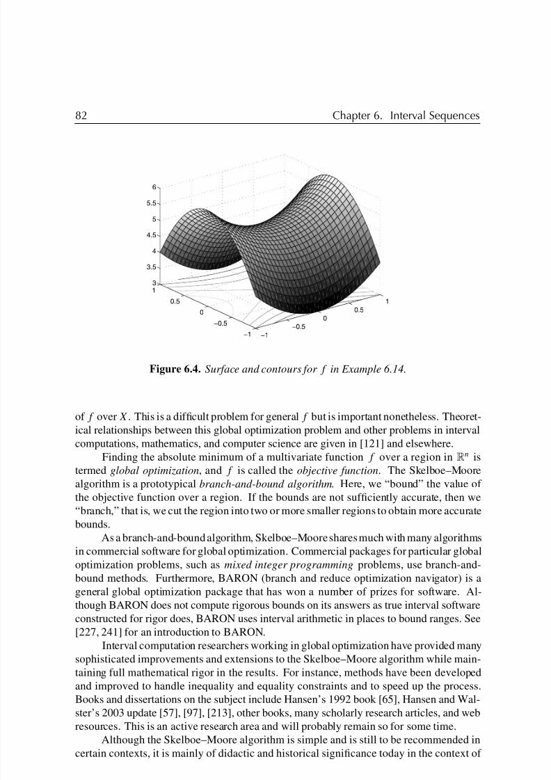
8/6/2019 Moore 1966
http://slidepdf.com/reader/full/moore-1966 93/234
82 Chapter 6. Interval Sequences
−1
−0.5
0
0.5
1
−1
−0.5
0
0.5
1
3
3.5
4
4.5
5
5.5
6
Figure 6.4. Surface and contours for f in Example 6.14.
of f over X. This is a difficult problem for general f but is important nonetheless. Theoret-
ical relationships between this global optimization problem and other problems in interval
computations, mathematics, and computer science are given in [121] and elsewhere.
Finding the absolute minimum of a multivariate function f over a region in Rn is
termed global optimization, and f is called the objective function. The Skelboe–Moore
algorithm is a prototypical branch-and-bound algorithm. Here, we “bound” the value of
the objective function over a region. If the bounds are not sufficiently accurate, then we
“branch,” that is, we cut the region into two or more smaller regions to obtain more accurate
bounds.
As a branch-and-bound algorithm, Skelboe–Moore shares much with many algorithms
in commercial software for global optimization. Commercial packages for particular global
optimization problems, such as mixed integer programming problems, use branch-and-
bound methods. Furthermore, BARON (branch and reduce optimization navigator) is a
general global optimization package that has won a number of prizes for software. Al-
though BARON does not compute rigorous bounds on its answers as true interval software
constructed for rigor does, BARON uses interval arithmetic in places to bound ranges. See
[227, 241] for an introduction to BARON.
Interval computation researchers working in global optimization have provided many
sophisticated improvements and extensions to the Skelboe–Moore algorithm while main-
taining full mathematical rigor in the results. For instance, methods have been developed
and improved to handle inequality and equality constraints and to speed up the process.Books and dissertations on the subject include Hansen’s 1992 book [65], Hansen and Wal-
ster’s 2003 update [57], [97], [213], other books, many scholarly research articles, and web
resources. This is an active research area and will probably remain so for some time.
Although the Skelboe–Moore algorithm is simple and is still to be recommended in
certain contexts, it is mainly of didactic and historical significance today in the context of
8/6/2019 Moore 1966
http://slidepdf.com/reader/full/moore-1966 94/234
6.5. Summary 83
global optimization. Algorithms in the above books, and algorithms tailored to specific
applications, described in various scholarly articles, generally are more practical today.
In the remainder of this section, we describe a few improvements to the Skelboe–Moore
algorithm.
For functions f having only one (or perhaps a few) isolated simple maximum or
minimum point(s) in X, we can use interval versions of Newton’s method to further reduce
the number of evaluations required to obtain sharp bounds on the range of values of f in
X. See also [210].
A clustering problem, perhaps first described in [44] and [102, 43], is the accumulation
of a large number of tiny boxes near a global minimum point of f (x1, . . . , xn). Thisphenomenon occurs, especially for large n. If interval Newton methods are used with
methods for finding local optimizers, the cluster problem can be avoided with a process
called epsilon inflation;26 see [97, section 4.2]. Also, the cluster problem can be avoided,
even for singular Hessian matrices, by astute selection of tolerances and construction of
boxes about approximate optimizers. A very early example of such an algorithm is Step 4 in
Algorithm 2.6 in [93]. Neumaier has further clarified the clustering problem mathematically,
and gives additional insight into how to avoid it; see [170].
We will give a few more details concerning global optimization in section 11.2.
6.5 SummaryAlgorithms based on refinements, discussed in this chapter, are used in interval software
to reduce overestimation, often in combination with other methods we will discuss in the
remaining chapters.
In the next chapter, we introduce interval computations in the context of numerical
linear algebra.
26The first use of the term “epsilon inflation” of which we are aware occurs in [218] as “ -Aufblähung,” near
the top of p. 99 of that work.

8/6/2019 Moore 1966
http://slidepdf.com/reader/full/moore-1966 95/234

8/6/2019 Moore 1966
http://slidepdf.com/reader/full/moore-1966 96/234
Chapter 7
Interval Matrices
7.1 Definitions
By an interval matrix, we mean a mean a matrix whose elements are interval numbers. For
example, we might have
A =
A11 A12
A21 A22
=
[1, 2] [−1, 1]
[0, 4] [6, 8]
. (7.1)
If A is an interval matrix with elements Aij and B is a matrix with real elements Bij such
that Bij ∈ Aij for all i and j , then we write B ∈ A.
Matrix Norm, Width, and Midpoint
We use the matrix norm
A = maxi
j
|Aij | (7.2)
for an interval matrix A. This is an interval extension of the maximum row sum norm for
real matrices. If B is any real matrix contained in an interval matrix A, then B ≤ A.
We define the width w(A) of an interval matrix A by
w(A) = maxi,j
w(Aij). (7.3)
The midpoint of A is the real matrix m(A) whose elements are the midpoints of the corre-
sponding elements of A:
(m(A))ij = m(Aij).
Clearly, m(A)∈A.
Example 7.1. For the interval matrix (7.1), we have
A = max{|[1, 2]| + |[−1, 1]| , |[0, 4]| + |[6, 8]|}
= max{2 + 1 , 4 + 8}
= 12,
85

8/6/2019 Moore 1966
http://slidepdf.com/reader/full/moore-1966 97/234
86 Chapter 7. Interval Matrices
w(A) = max{w([1, 2]), w([−1, 1]), w([0, 4]), w([6, 8])}
= max{1, 2, 4}
= 4,
and
m(A) =
m([1, 2]) m([−1, 1])
m([0, 4]) m([6, 8])
=
0.5 0
2 7
.
Exercise 7.1. Show that the product of two interval matrices using interval arithmetic is
again an interval matrix consisting of interval elements each of which is exactly the range of
values of the corresponding element of the product of a pair of real matrices whose elements
are chosen independently from the corresponding elements of the interval matrices.
7.2 Interval Matrices and Dependency
Even though, as indicated in Exercise 7.1, the ijth element Cij of the product C = AB of
an m by p interval matrix A and a p by n interval matrix B gives sharp bounds on the range
Cij = M ij =
p
k=1
P ik Qkj : P ik ∈ Aik and Qkj ∈ Bkj for 1 ≤ k ≤ pfor each i, 1 ≤ i ≤ m, and each j , 1 ≤ j ≤ n, the resulting interval matrix C may contain
point matrices D that are not the result of the multiplication of point matrices P ∈ A and
Q ∈ B. The multiplication of practically any two interval matrices such that the second
matrix has more than one column can serve as an example.
Example 7.2. Consider
A =
[1, 2] [3, 4]
and B =
[5,6] [7,8]
[9,10] [11,12]
.
Then the product of the interval matrices A and B is
C = AB =
[32,52] [40,64]
.
However, D = (32 64) ∈ C, but D does not correspond to the product of any point matrix
P ∈ A with any point matrix Q ∈ B. In fact, the first element 32 of D is taken by taking
the product of the lower bound matrix A = (1 3) ∈ A with the lower bounds (5 9)T of
the first column of B, while the second element of D is obtained by taking the upper bound
matrix A ∈ A with the upper bounds (8 12)T of the second column of B. This type of
interval dependency occurs because the interval arithmetic does not assume that the same
point elements are chosen from the interval elements of A in forming the sets comprising thedifferent columns of the product interval matrix C. This is similar to interval dependency
in scalar expressions, as introduced on p. 38 and treated in the Fundamental Theorem of
Interval Analysis (Theorem 5.1). In terms of the Fundamental Theorem, if you think of each
interval element of the left matrix A as being a variable, then this variable occurs multiple
times, once for each column, in forming the columns of the interval product matrix C.

8/6/2019 Moore 1966
http://slidepdf.com/reader/full/moore-1966 98/234
7.3. INTLAB Support for Matrix Operations 87
7.3 INTLAB Support for Matrix Operations
INTLAB has extensive support for linear algebra operations involving interval matrices.
INTLAB uses the MATLAB environment, which originated as a system for interactively
doing numerical linear algebra and continues to have numerical linear algebra as its foun-
dation. The following exercises deal with some elementary matrix and norm capabilities in
INTLAB.
Exercise 7.2. Several functions of intervals are related to the absolute value function of a
real number.
mag: mag(X), the magnitude of the interval X, is the real number representing the maxi-
mum absolute value of any real number in X.
mig: mig(X), the mignitude of the intervalX, is the real number representing the minimum
absolute value of any real number in X. (For example, the mignitude is used, in
determining whether every matrix within an interval matrix is diagonally dominant.)
abs: abs(X) is an interval that represents the range of the absolute value function over the
interval X.
INTLAB has the functions mag, mig, and abs that operate on intervals, interval vectors,
and interval matrices. Use INTLAB to compute abs(X), mag(X), and mig(X) for the
following X:
1. X = [1, 2],
2. X = [−1, 2],
3. X = [−2,−1],
4. X the matrix A from Example 7.1.
Hint : The matrix A may be entered:
>> A = [infsup(1,2) infsup(-1,1)
infsup(0,4) infsup(6,8)]
intval A =
[ 1.0000 , 2.0000 ] [ -1.0000 , 1.0000 ]
[ 0.0000 , 4.0000 ] [ 6.0000 , 8.0000 ]
Exercise 7.3. INTLAB implements norm and midpoint for matrices with the functions norm
and mid, respectively. The function norm is an extension of the MATLAB function that
computes the norm of a matrix. If A is a real matrix, then norm(A) in MATLAB computes
the 2-norm of A and is the same as norm(A,2), while norm(A,1) and norm(A,inf)
compute the 1-norm and ∞-norm of A, respectively. INTLAB does not define norm(A,2)when A is an interval matrix, but it does define norm(A,1) and norm(A,inf); the norm
defined in (7.2) corresponds to mag(norm(A,inf)). (The command norm(A) does not
work when A is an interval matrix.) The midpoint matrix for a matrix A cannot be the exact
midpoint matrix, but it is a floating point approximation. Use INTLAB to compute A
and m(A) for A as in Example 7.1.

8/6/2019 Moore 1966
http://slidepdf.com/reader/full/moore-1966 99/234
88 Chapter 7. Interval Matrices
Exercise 7.4. For scalar intervals, the INTLAB function diam corresponds to width. How-
ever, diam acts componentwise, returning a matrix when acting on a matrix.
(a) For A the matrix of Example 7.1, issue the following commands:
(i) diam(A),
(ii) max(diam(A)),
(iii) max(max(diam(A))).
Explain each result. ( Hint : Look up max in MATLAB’s help system.)
(b) Using this experimentation, write a MATLAB function wid.m, callable by width
= wid(A), such that the returned value is the width of the matrix A as defined by
(7.3).
7.4 Systems of Linear Equations
In this section, we consider finite systems of linear algebraic equations
Ax = b, (7.4)
where A is an n-by-n matrix and b is an n-dimensional vector. There are two cases to
consider for the coefficients of A and b:
(1) they are real numbers exactly representable by machine numbers, and
(2) they are only known to lie in certain intervals Aij and Bi .
There are two types of methods for the numerical solution of such problems. Direct
methods, such as Gaussian elimination (with or without various “pivoting” schemes) can
produce exact results in case 1 in a finite number of arithmetic operations if A is nonsingular
and if infinite precision arithmetic is used. Indirect (or iterative) methods for the solution of
(7.4) in case 1 produce a sequence of approximate solutions which converge to the uniquesolution if, for instance, A is of the form
A = I − M,
where I is the identity matrix and M has norm less than 1, such as for the norm (maximum
row sum norm)
M = maxi
j
|M ij |. (7.5)
An exact solution in case (2) is much more difficult; the set of all solutions to (7.4),
when the coefficients of A and b can range over intervals, may be a very complicated set,27
and its computation is, in general, an NP-hard problem [121]. An example of such a solution
set, with
A =
[ 2, 4] [−2, 1]
[−1, 2] [ 2, 4]
, B =
[−2, 2]
[−2, 2]
, (7.6)
27See, for instance [97, section 1.2.1] and the references there for a discussion of different kinds of solution sets.

8/6/2019 Moore 1966
http://slidepdf.com/reader/full/moore-1966 100/234
7.4. Systems of Linear Equations 89
T
E r
r
r r
r
r
r
r
¨ ¨ ¨ ¨ ¨ ¨ d
d d
d d e e e e e e
¨ ¨ ¨ ¨
¨ ¨ d d d
d de
e e e e e
(1, 0)
(3,−4)
(4, 3)(0, 1)
¢ ¢ ¢
(−3, 4)
(−1, 0)
(−4,−3)
(0,−1)
Figure 7.1. Exact solution set to Ax = B , A , and B in Equation (7.6).
appears in Figure 7.1 (from [97, p. 20]). However, such a solution set can be enclosed in an
interval vector (an n-dimensional rectangle). As an immediate consequence of Corollary
5.1, we have the following computable test for existence of solutions to (7.4), with real or
interval coefficients.
Theorem 7.1. If we can carry out all the steps of a direct method for solving (7.4) in IA (if no attempted division by an interval containing zero occurs, nor any overflow or underflow),
then the system (7.4) has a unique solution for every real matrix in A and every real vector
in b, and the solution is contained in the resulting interval vector X.
Consider the general 2-by-2 linear system
a11x1 + a12x2 = b1,
a21x1 + a22x2 = b2.
Formally, we can eliminatex1 from the second equation by subtracting term by terma21/a11
times the first equation, as done in Gaussian elimination. Doing that, we can solve for x2
by a division from the equation
(a22 − (a21/a11)a12)x2 = b2 − (a21/a11)b1.
Then we can use that value of x2 and the first equation to solve for x1 by another division
from
a11x1 = b1 − a12x2.
We can carry out all that numerically with interval coefficients for all the a’s and b’s to obtain
intervals X1 and X2 containing all the possible solutions (x1, x2) for any choices of real
coefficients in the corresponding interval coefficients. All this can be done if the intervalfor a11 does not contain zero and if the computed interval containing a22 − (a21/a11)a12
does not contain zero.
The determinant of the matrix is the product of those two quantities: a11(a22 −
(a21/a11)a12). The conditions stated above are sufficient for the matrix to be nonsingu-
lar for any choice of real coefficients in the interval coefficients.
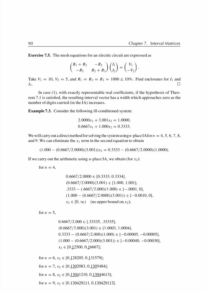
8/6/2019 Moore 1966
http://slidepdf.com/reader/full/moore-1966 101/234
90 Chapter 7. Interval Matrices
Exercise 7.5. The mesh equations for an electric circuit are expressed as
R1 + R2 −R2
−R2 R2 + R3
I 1
I 2
=
V 1
−V 2
.
Take V 1 = 10, V 2 = 5, and R1 = R2 = R3 = 1000 ± 10%. Find enclosures for I 1 and
I 2.
In case (1), with exactly representable real coefficients, if the hypothesis of Theo-
rem 7.1 is satisfied, the resulting interval vector has a width which approaches zero as the
number of digits carried (in the IA) increases.
Example 7.3. Consider the following ill-conditioned system:
2.0000x1 + 3.001x2 = 1.0000,
0.6667x1 + 1.000x2 = 0.3333.
We will carry out a direct method for solving the system using n-place IAfor n = 4, 5, 6, 7, 8,
and 9. We can eliminate the x1 term in the second equation to obtain
(1.000 − (0.6667/2.0000)(3.001))x2 = 0.3333 − (0.6667/2.0000)(1.0000).
If we carry out the arithmetic using n-place IA, we obtain (for x2):
for n = 4,
0.6667/2.0000 ∈ [0.3333, 0.3334],
(0.6667/2.0000)(3.001) ∈ [1.000, 1.001],
.3333 − (.6667/2.000)(1.000) ∈ [−.0001, 0],
(1.000 − (0.6667/2.0000)(3.001)) ∈ [−0.0010, 0],
x2 ∈ [0,∞) (no upper bound on x2);
for n = 5,
0.6667/2.000 ∈ [.33335, .33335],
(0.6667/2.000)(3.001) ∈ [1.0003, 1.0004],
0.3333 − (0.6667/2.000)(1.000) ∈ [−0.00005,−0.00005],
(1.000 − (0.6667/2.000)(3.001)) ∈ [−0.00040,−0.00030],
x2 ∈ [0.12500, 0.16667];
for n = 6, x2 ∈ [0.128205, 0.131579];
for n = 7, x2 ∈ [0.1302083, 0.1305484];
for n = 8, x2 ∈ [0.13041210, 0.13044613];
for n = 9, x2 ∈ [0.130429111, 0.130429112].
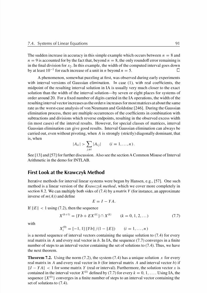
8/6/2019 Moore 1966
http://slidepdf.com/reader/full/moore-1966 102/234

8/6/2019 Moore 1966
http://slidepdf.com/reader/full/moore-1966 103/234
92 Chapter 7. Interval Matrices
Example 7.4. Consider (7.4) with
A =
3 1
3 2
, b =
1
0
.
If we choose
Y =
0.6 −0.3
−1 1
, an approximate inverse of A,
we find, using three-digit IA,
E =
0.1 00 0
, Y b =
0.6−1
, X(0)
=[−1.12, 1.12][−1.12, 1.12]
,
and we obtain
X(1)=
[0.478, 0.712]
−1
, X(2)
=
[0.647, 0.672]
−1
,
X(3)=
[0.664, 0.668]
−1
, X(4)
=
[0.666, 0.667]
−1
,
with X(k)
= X(4)
for k ≥ 4.
The iterative method (7.7) is also applicable in case A and b have interval components.
Alternate methods and methods that give sharper bounds on the set of solutions to linear
systems with interval coefficients may be found in [13], [57], [218], and [221]. Method
(7.7) is a linear version of the Krawczyk method that we will explain in more detail in
section 8.2. In fact, because nonlinearities in a system can be encompassed by intervals in
a linear system, as we shall see in the next chapter, in some contexts there is less distinction
between interval methods for linear systems and interval methods for nonlinear systems
than there is with point methods.
Additional Notes
1. We will say more about convergence of the Krawczyk method in section 8.2.
2. Better enclosures of the solution can be obtained in practice througha defect-correction
scheme than with just the simple method we have presented here. This was observed
in [218, section 2.b, p. 53], was later explained in [221], and is implemented within
routine verifylss in INTLAB.
7.5 Linear Systems with Inexact DataThere are a few special types of matrices for which satisfactory results can be obtained.
Unfortunately, the use of direct methods, such as Gaussian elimination with interval arith-
metic, cannot be recommended in the general case for finding enclosures of the set of all
solutions to linear systems with inexact data, represented by interval coefficients. Bounds
of intermediate quantities tend to grow rapidly especially because of dependence among

8/6/2019 Moore 1966
http://slidepdf.com/reader/full/moore-1966 104/234
7.5. Linear Systems with Inexact Data 93
generated intervals and the endpoint reversals occurring in subtractions. The exact solution
set can be quite complicated, but we can nevertheless compute an enclosure of it, using the
iterative method outlined in the previous section. Let us revisit Exercise 7.5 to illustrate its
application.
Example 7.5. The mesh equations for an electric circuit are expressed asR1 + R2 −R2
−R2 R2 + R3
I 1
I 2
=
V 1
−V 2
with V 1 = 10, V 2 = 5, and R1 = R2 = R3 = 1000 ± 10%. We can use the iterative method
(7.7) to find enclosures for I 1 and I 2. In this example, the matrix A in (7.7) can be written
A =
[1800, 2200] −[900, 1100]
−[900, 1100] [1800, 2200]
,
and the right-hand side vector is
b =
10
−5
.
Now the midpoint matrix is
m(A) = 2000 −1000
−1000 2000 = 2000 1 − 1
2
−12 1
,which has the inverse
[m(A)]−1 =1
2000
43
23
23
43
=
4
60002
6000
26000
46000
=
6.666 . . . × 10−4 3.333 . . . × 10−4
3.333 . . . × 10−4 6.666 . . . × 10−4
.
It is not necessary to find the exact inverse, although in this simple case, we can do it. In
fact, it will suffice to choose as our approximation to [m(A)]−1 the matrix
Y = 10−4
6 3
3 6
.
What we need is a matrix Y that makes the norm of E = I − YA smaller than 1, and the
smaller the better. Here, we have
E =
1 0
0 1
−
6 3
3 6
[0.1800, 0.2200] −[0.0900, 0.1100]
−[0.0900, 0.1100] [0.1800, 0.2200]
= [−0.05, 0.25] [−0.12, 0.12]
[−0.12, 0.12] [−0.05, 0.25] ,so E = 0.37 < 1. It follows that we can obtain a nested sequence of enclosures of the set
of solutions to the linear system with inexact data (known only to be in the given intervals),
from the iterative method (7.7), beginning with
X(0) =Yb
1 − E
[−1, 1]
[−1, 1]
,
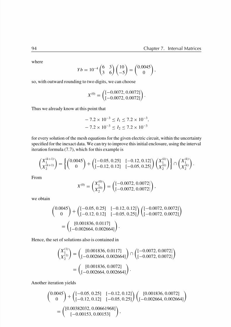
8/6/2019 Moore 1966
http://slidepdf.com/reader/full/moore-1966 105/234

8/6/2019 Moore 1966
http://slidepdf.com/reader/full/moore-1966 106/234
7.5. Linear Systems with Inexact Data 95
so the set of solutions is also contained inX
(2)1
X(2)
2
=
[0.00382032, 0.00661968]
[−0.00153, 0.00153]
∩
[0.001836, 0.0117]
[−0.002664, 0.002664]
=
[0.00382032, 0.00661968]
[−0.00153, 0.00153]
.
We could continue the iterations to further sharpen the enclosure. The computations dis-
played above illustrate the interval operations needed.
For this example, we can compare the enclosure above with the one found in the
solution of Exercise 7.5. Using a direct method for this small linear system, we found the
sharper enclosure
I 1 = [0.00433, 0.00582], I 2 = [−0.000419, 0.000419].
Exercise 7.6. Use INTLAB to check the above computations. Hint : There are severalways of doing this. One is to check the computations directly by entering the matrices andvectors, then doing the matrix-vector multiplications, taking midpoints, inversions, etc., inINTLAB. You can also use the function Krawczyk_step displayed on p. 118 with y = 0and f(y) = Ay − b, but you will need to check the starting vector separately. Here is a setof commands to get you started:
A = [infsup(1800,2200), -infsup(900,1100);...-infsup(900,1100), infsup(1800,2200)]
B = [10;-5]
Y = 10ˆ(-4) * [6 3; 3 6]
E = eye(2) - Y*A
xmult = norm(Y*B)/(1-mag(norm(E,inf)))
X = xmult * [infsup(-1,1);infsup(-1,1)]
(Above, you see mag(norm(E,inf)) because INTLAB computes the matrix norm as aninterval, and mag(norm(E,inf)) corresponds to the matrix norm we have defined.) Youcan then duplicate the first step of the above computations via
X1 = Y*B + E*X
etc. Alternately, to use Krawczyk_step, issue the line
X = intersect(Krawcayk_step(X,[0.0],’example7p5’),X)
where example7p5 (also supplied) is as follows:
function [val] = example7p5(x)
% [y] = example7p5(x) implements Example 7.5 for
% Krawczyk_step
A = [ infsup(1800,2200) -infsup(900,1100)
-infsup(900,1100) infsup(1800,2200)];
b = [midrad(10,0);midrad(-5,0)];val = A*x - b;
You can then iterate the Krawczyk method by pressing the up-arrow key followed by the
return key. However, the results from Krawczyk_step will differ a bit from those on the
preceding pages, because Krawczyk_step uses a more accurate approximation to m(A)−1
for Y . (See p. 200 for other possible discrepancies.)

8/6/2019 Moore 1966
http://slidepdf.com/reader/full/moore-1966 107/234
96 Chapter 7. Interval Matrices
Exercise 7.7. The INTLAB routine verifylss computes verified enclosures to linear
systems of equations using a combination of the Krawczyk method and an improved method
originating from work of Hansen, [218], and [184], [168]; type help verifylss from
the MATLAB command window for more information. Use verifylss on the linear
system just worked out in Example 7.5 and compare the results you obtain with the above
results.
An Additional Note As mentioned, we will treat the Krawczyk method more generally
in section 8.2, starting on p. 116. There, we treat it as a method for bounding the solutions
to nonlinear systems as well as give additional background.
Interval Gauss–Seidel
An alternate method, also commonly used in practice, was originally introduced by Hansen
et al. in the Hansen–Sengupta method [66] and is an interval version of classical Gauss–
Seidel iteration. As in the Krawczyk method, assume A is an interval matrix, B is an interval
vector (where either A or B can have zero width or nonzero width), and we wish to bound
the solution set to
Ax = B. (7.8)
We use a preconditioner matrix Y typically but not necessarily chosen to be m(A)−1 (see
[97, Chapter 3]), obtaining
Gx = C, where G = Y A and C = Y B. (7.9)
Formally solving the ith row of the preconditioned system (7.9) for xi , and assuming we
iterate to obtain a new range for Xi by substituting the ranges for Xj , j = i, using the
most recent value of Xj wherever possible, we obtain the iteration equations for the interval
Gauss–Seidel method:
X(0)i is given, 1 ≤ i ≤ n,
X(k+1)i ←
1
Gi,i
Ci −
i−1j =1
Gi,j X(k+1)j −
nj =i+1
Gi,j X(k)j
, i = 1, 2, . . . , n,
X(k+1)i ← X
(k+1)i ∩ X
(k)i ,
(7.10)
where G = {Gi,j }.In the Krawczyk method, as long as a preconditioner matrix Y is available, the iteration
(7.7) contains no divisions and consists of a single box. However, it could happen that
0 ∈ Gi,i , where the diagonal element Gi,i of G is the denominator in (7.10); thus, analogousto what we will see in section 8.1 for the univariate interval Newton method, extendedinterval arithmetic can be used, and the result of a step of (7.10) can be two boxes. Thefollowing m-file computes a step of (7.10) for a single i without intersecting. (That is,gauss_seidel_step evaluates the right side of the middle assignment in (7.10) for agiven i.) The preconditioner is not given as a matrix but rather is given as a row Y i to allowthe preconditioner matrix to be computed rowwise, as explained in [97, Chapter 3]. The

8/6/2019 Moore 1966
http://slidepdf.com/reader/full/moore-1966 108/234
7.5. Linear Systems with Inexact Data 97
result of a division by zero is computed according to the Cset theory of [194], using thevariant that views −∞ and ∞ as part of the number system. (We explain Cset theory onp. 113.)
function [new_X_i, second_new_X_i, there_are_2,...
numerator, denominator]...
= gauss_seidel_step(i, Y_i, A, B, X)
% [new_X_i, second_new_X_i, there_are_2]...
% = gauss_seidel_step(i, Y_i, A, B, X) returns
% the result of applying a Gauss--Seidel step with variable i,
% preconditioner matriX Y_i, and initial guess X. The variable% there_are_2 is set to 1 if 2 semi-infinite intervals are returned,
% in which case second_new_X_i has the second interval; there_are_2
% is set to 0 and second_new_X_i is not set if there is only
% one interval returned.
n = size(A,2);
G_i = Y_i*A;
C_i = Y_i*B;
numerator = C_i;
new_X_i = X(i);
second_new_X_i = X(i);i f ( n > 1 )
i f ( i > 1 )
numerator = numerator - G_i(1:i-1)*X(1:i-1);
end
i f ( i < n )
numerator = numerator - G_i(i+1:n)*X(i+1:n);
end
end
denominator = G_i(i);
numerator;
denominator;if (˜in(0,denominator))
there_are_2 = 0;
new_X_i = numerator / denominator;
elseif (˜in(0,numerator))
there_are_2 = 1;
supnum = sup(numerator);
if(supnum < 0)
if sup(denominator)==0
tmp1 = infsup(-Inf,-Inf);
else
tmp1 = midrad(supnum,0) / midrad(sup(denominator),0);end
if inf(denominator) == 0
tmp2 = infsup(Inf,Inf);
else
tmp2 = midrad(supnum,0) / midrad(inf(denominator),0);
end

8/6/2019 Moore 1966
http://slidepdf.com/reader/full/moore-1966 109/234
98 Chapter 7. Interval Matrices
new_X_i = infsup(-Inf,sup(tmp1));
second_new_X_i = infsup(inf(tmp2),inf);
else
infnum = inf(numerator);
if inf(denominator)==0
tmp1 = infsup(-Inf,-Inf)
else
tmp1 = midrad(infnum,0) / midrad(inf(denominator),0);
end
if sup(denominator) == 0
tmp2 = infsup(Inf,Inf)else
tmp2 = midrad(infnum,0) / midrad(sup(denominator),0);
end
new_X_i = infsup(-Inf,sup(tmp1));
second_new_X_i = infsup(inf(tmp2),Inf);
end
else
there_are_2=0;
new_X_i = infsup(-Inf,Inf);
end
end
The following m-file repeatedly calls gauss_seidel_step to do an entire sweep of
(7.10), that is, to compute X(k+1)i , 1 ≤ i ≤ n, given X
(k)
i , 1 ≤ i ≤ n:
function [X_kp1,is_empty, error_occurred] =...
Gauss_Seidel_image(A, B, X_k)
% X_kp1] = Gauss_Seidel_image(A,B,X_k) returns the image after a
% sweep of Gauss--Seidel iteration ( that is, (7.8) of the text)
% for the interval linear system A X = B, beginning with box X_k,
% 1 < = i < = n .
% This is done using the inverse midpoint preconditioner.
% Upon return:% if error_occurred = 1, then the computation could not proceed.
% (For example, the midpoint preconditioner may have been
% singular, or the denominator may have contained zero; the
% case of more than one box in the image is not handled
% with this routine.) Otherwise, error_occurred = 0.
% If error_occurred = 0 but is_empty = 1, this means that
% an intersection of a coordinate extent was empty. In this
% case, there are no solutions to A X = B within X_k.
% If error_occurred = 0 and is_empty = 0, then the image under
% the Gauss--Seidel sweep is returned in X_kp1.
n = length(B);
Y = inv(mid(A));
error_occurred = 0;
is_empty = 0;
i=1;
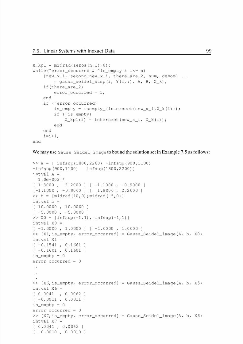
8/6/2019 Moore 1966
http://slidepdf.com/reader/full/moore-1966 110/234
7.5. Linear Systems with Inexact Data 99
X_kp1 = midrad(zeros(n,1),0);
while(˜error_occurred & ˜is_empty & i<= n)
[new_x_i, second_new_x_i, there_are_2, num, denom] ...
= gauss_seidel_step(i, Y(i,:), A, B, X_k);
if(there_are_2)
error_occurred = 1;
end
if (˜error_occurred)
is_empty = isempty_(intersect(new_x_i,X_k(i)));
if (˜is_empty)
X_kp1(i) = intersect(new_x_i, X_k(i));end
end
i=i+1;
end
We may use Gauss_Seidel_image to bound the solution set in Example 7.5 as follows:
>> A = [ infsup(1800,2200) -infsup(900,1100)
-infsup(900,1100) infsup(1800,2200)]
intval A =
1.0e+003 *[ 1.8000 , 2.2000 ] [ -1.1000 , -0.9000 ]
[-1.1000 , -0.9000 ] [ 1.8000 , 2.2000 ]
>> b = [midrad(10,0);midrad(-5,0)]
intval b =
[ 10.0000 , 10.0000 ]
[ -5.0000 , -5.0000 ]
>> X0 = [infsup(-1,1), infsup(-1,1)]
intval X0 =
[ -1.0000 , 1.0000 ] [ -1.0000 , 1.0000 ]
>> [X1,is_empty, error_occurred] = Gauss_Seidel_image(A, b, X0)
intval X1 =[ -0.1541 , 0.1661 ]
[ -0.1601 , 0.1601 ]
is_empty = 0
error_occurred = 0
.
.
.
>> [X6,is_empty, error_occurred] = Gauss_Seidel_image(A, b, X5)
intval X6 =
[ 0.0041 , 0.0062 ]
[ -0.0011 , 0.0011 ]is_empty = 0
error_occurred = 0
>> [X7,is_empty, error_occurred] = Gauss_Seidel_image(A, b, X6)
intval X7 =
[ 0.0041 , 0.0062 ]
[ -0.0010 , 0.0010 ]

8/6/2019 Moore 1966
http://slidepdf.com/reader/full/moore-1966 111/234

8/6/2019 Moore 1966
http://slidepdf.com/reader/full/moore-1966 112/234
7.7. Sparse Linear Systems Within INTLAB 101
element should be chosen, since the pivots become intervals.30 Indeed, it is likely that all
potential pivots in the j th column will contain zero at some step, due to magnification of
widths, so that production of finite bounds on the solution becomes impossible.
There are various ways in which Gaussian elimination can be used to get tight bounds
on the solutions to point systems of linear equations. For instance, one may precondition,
just as we did for the interval Gauss–Seidel method or, in a way, with the matrix Y in the
Krawczyk method. That is, we first use floating point arithmetic to produce an approximate
inverse Y ≈ A−1, then use interval arithmetic to do the matrix-matrix multiplication and
matrix-vector multiplication, to produce an interval matrix G that contains the exact matrix
YA and an interval vectorC that contains the exact vectorYb. The solution set to the systemof equations Gx = C must then contain the exact solution to the original noninterval system
Ax = b. The Gaussian elimination algorithm can then be performed on Gx = C, leading
to reasonable bounds on the solution set to Ax = b.
If the original systemAx = B is an interval system of equations, that is, if the elements
of the matrix A and the vector B have nonzero widths at the start, we may multiply by a
preconditioner matrix Y ≈ m(A)−1, just as we did for the interval Gauss–Seidel method.
The Gaussian elimination algorithm is then more likely to succeed for the resulting system
of equations.
Interval Gaussian elimination is analyzed theoretically in [12], [13], and [167] as well
as in other papers and reference works.
7.7 Sparse Linear Systems Within INTLAB
MATLAB has a sparse matrix format, and the routines in INTLAB (and in particular
verifylss) can use this sparse format. Depending upon how wide the intervals are,
the structure of the matrix, and the condition of the matrix, meaningful answers can be
obtained for some very large matrices. Here, we will give an example with cursory ex-
planation; complete understanding of this example can be obtained by studying the sparse
matrix format within MATLAB’s help system.
Example 7.6. Suppose we wish to bound the solutions to Ax = b, where A is the 1000 by
1000 matrix given by
A =
[2.9999, 3.0001] −1 0 · · ·
−1 [2.9999, 3.0001] −1 0 · · ·
.... . .
0 · · · 0 −1 [2.9999, 3.0001]
,
and b ∈ R1000 has all entries equal to −1. If such a matrix is passed to verifylss,
there is an implicit assumption that the diagonal entries vary independently, that is, that the
diagonal matrices A are xi where, in general xi = xj , although each xi lies in the interval
30One way of choosing a pivot element during the j th step would be to choose Ai0,j to be the pivot row, where
i0 = argmaxi
mig(Ai,j )
, where “mig” is the mignitude defined on p. 87.

8/6/2019 Moore 1966
http://slidepdf.com/reader/full/moore-1966 113/234
102 Chapter 7. Interval Matrices
[2.9999, 3.0001]. (If the diagonal entries are all the same value, even though that value is
known to lie only within [2.9999, 3.0001], then sharper bounds on the solution set possibly
can be obtained by taking account of this fact.)A MATLAB dialogue that gives us bounds on the solution set follows:
>> n = 1000;
>> intvalinit(’Display_’)
>> for i=1:n;b(i,1)=-1;end;
>> diag_uncertainty = midrad(3,1e-4)
intval diag_uncertainty = 3.0000__________
>> for i=1:n;B(i,1) = midrad(-1,0);
B(i,2)=diag_uncertainty;
B(i,3) = midrad(-1,0);end
>> d = [-1;0;1];
>> A = spdiags(B,d,n,n);
>> A(1:3,1:3)
intval ans =
(1,1) 3.0000__________
(2,1) -1.00000000000000
(1,2) -1.00000000000000
(2,2) 3.0000__________
(3,2) -1.00000000000000(2,3) -1.00000000000000
(3,3) 3.0000__________
>> X=verifylss(A,b);
>> X(1:4)
intval ans =
-0.62____________
-0.85____________
-0.94____________
-0.98____________
>> X(500:503)
intval ans =-1.00____________
-1.00____________
-1.00____________
-1.00____________
>> X(997:1000)
intval ans =
-0.98____________
-0.94____________
-0.85____________
-0.62____________
The response and solution process in this interactive dialogue were almost immediate
(small fractions of a second).
Material on mathematically rigorous bounds to solutions of sparse systems of equa-
tions can be found in [221] and [226].

8/6/2019 Moore 1966
http://slidepdf.com/reader/full/moore-1966 114/234
7.8. Final Notes 103
7.8 Final Notes
Mayer, Alefeld, Rohn, and others have made significant advances in characterizing the
solution sets to interval linear systems. These results include characterizing necessary
and sufficient conditions for when interval Gaussian elimination and other algorithms for
bounding solution sets can be carried out and when they give sharp enclosures for the
solution sets. They also include results for interval matrices with assumed dependency in
their entries, such as for symmetric, persymmetric, Toeplitz, and Hankel matrices. Günter
Mayer provided an excellent review of this in [140].
Jiri Rohn, aside from his role as a leader in these developments and in the analysis
of computational complexity in interval numerical linear algebra, has made available a
sizeable suite of INTLAB programs for interval linear systems of equations. He has written
a concise summary of results on interval linear problems. See Appendix D.
In the next chapter, the ideas and techniques discussed in Chapters 6 and 7 are used to
develop methods for mathematically rigorous bounds on the solutions to nonlinear systems
of equations.

8/6/2019 Moore 1966
http://slidepdf.com/reader/full/moore-1966 115/234

8/6/2019 Moore 1966
http://slidepdf.com/reader/full/moore-1966 116/234
Chapter 8
Interval Newton Methods
In Chapter 6, we discussed iterative interval methods for solving equations in fixed-point
form. Given an equation
x = f (x), (8.1)
we take an interval extension F of f (which is automatically inclusion isotonic if f is
rational) and set up an iterative procedure of the form
Xk+1 = F(Xk) ∩Xk (k = 0, 1, 2, . . . ) . (8.2)
If we start with an X0 such that F(X0) ⊆ X0, then (8.2) produces a nested sequence of
intervals {Xk} convergent to an interval X∗ such that X∗ = F(X∗) and X∗ ⊆ Xk for all
k = 0, 1, 2, . . .. On a computer, the procedure can be halted when Xk+1 = Xk ; using IA
at a specific number of digits, this yields the narrowest interval possible (with that many
digits) containing X∗.
The Krawczyk method, considered in Chapter 6 in the linear case, falls under the
same general scheme as (8.2) and can be used to solve nonlinear systems of equations.More generally, interval Newton methods share properties with the Krawczyk method, can
be implemented with iteration (8.2), and can be used to prove existence and uniqueness of a
solution to a nonlinear system of equations in a given box, even though the interval Newton
operator is not inclusion isotonic as is F in (8.2). We describe these methods below.
8.1 Newton’s Method in One Dimension
Our approach will be to initially develop Newton’s method in its simplest form. Let f be a
real-valued function of a real variable x, and suppose that f is continuously differentiable.
By the mean value theorem, we can write
f(x) = f(y)+ f (s)(x − y) (8.3)
for some s between x and y. Now let [a, b] be an interval in which we seek a solution of
the equation
f(x) = 0. (8.4)
105

8/6/2019 Moore 1966
http://slidepdf.com/reader/full/moore-1966 117/234
106 Chapter 8. Interval Newton Methods
A solution x, if it exists, would satisfy
f(y) + f (s)(x − y) = 0 (8.5)
for any y ∈ [a, b], in particular for y = m([a, b]) = (a + b)/2. Hence,
x = y − f (y)/f (s). (8.6)
Let F (X) be an inclusion monotonic interval extension of f (x) and consider the algorithm
X(k+1)
=X(k)
∩N(X(k)) (k
=0, 1, 2, . . . ) , (8.7)
where
N(X) = m(X) − f (m(X))/F (X). (8.8)
It follows from (8.6) that x is contained in N(X) if y = m(X), and if x is contained in X,
then s in (8.3) is also contained in X. In this case, x is also contained in X(k) for all k if it
is contained in X(0). We have the following theorem.
Theorem 8.1. If an interval X(0) contains a zero x of f(x), then so does X(k) for all
k = 0, 1, 2, . . ., defined by (8.7). Furthermore, the intervals X(k) form a nested sequence
converging to x if 0 /∈ F (X(0)).
Proof. If 0 /∈ F (X(0)), then 0 /∈ F (X(k)) for all k and m(X(k) ) is not contained in N (X(k) ),
unless f (m(X(k) ) = 0. Therefore w(X(k+1)) < 12
w(X(k)). Convergence of the sequence
follows.
Exercise 8.1. What happens if f (m(X(k) ) = 0?
Example 8.1. Suppose we wish to solve (8.4) with
f(x) = x2 − 2. (8.9)
An interval extension of f (x)
=2x is F (X)
=2X. Hence,
N(X) = m(X) − [m(X)]2 − 2
2X,
and (8.7) looks like
X(k+1) = X(k) ∩
m(X(k)) − [m(X(k))]2 − 2
2X(k)
.
Taking X(0) = [1, 2], we obtain
X(1)
= [22
16, 23
16 ],
X(2) = [1.41406 . . . , 1.41441 . . .],
X(3) = [1.414213559 . . . , 1.414213566 . . .].
Of course, (8.4) has solution x =√
2. Rounding X(3) out at the eighth place, we see that√ 2 lies in [1.41421355, 1.41421357].

8/6/2019 Moore 1966
http://slidepdf.com/reader/full/moore-1966 118/234

8/6/2019 Moore 1966
http://slidepdf.com/reader/full/moore-1966 119/234
108 Chapter 8. Interval Newton Methods
If the intersection X(k) ∩ N(X(k)) in (8.7) is empty, there is no zero of f in X(k) .
Exercise 8.3. Illustrate this by taking X(0) = [4, 6] in Example 8.1.
Example 8.2. The iteration equation (8.7) can be implemented easily with INTLAB in thefollowing m-file i_newton_step.m:
function [NX_intersect_X, is_empty] = i_newton_step(f,f_prime,X)
% [NX_intersect_X, is_empty] = i_newton_step(f,f_prime,X)
% returns the result of a single step of the interval Newton
% method for a single variable, as defined in (8.8) of
% the text, using X as initial interval. The string f should% be the name of an "m" file for evaluating the function,
% while the string "f_prime" should be the name of an "m"
% file for evaluating the derivative of f. The flag "is_empty"
% is set to "0" if the intersection is non-empty, and is set
% to "1" if the intersection is empty.
midX = infsup(mid(X),mid(X));
NX = midX - feval(f,midX) / feval(f_prime,X)
NX_intersect_X = intersect(NX,X);
is_empty = isempty_(NX_intersect_X);
The function in Example 8.1 can be implemented in the following two m-files:
function [y] = example8p1(x);
% y = example8p1(x) returns xˆ2 -2 in y, regardless of the
% variable type of x; y will be of the same variable type
% a s x .
y = x . ˆ 2 - 2 ;
and
function [y] = example8p1_prime(x);
% y = example8p1(x) returns the derivative of xˆ2 -2 in y,
% regardless of the variable type of x; y will be of the
% same variable type as x.
y = 2*x;
With these three m-files, we may produce the following MATLAB console dialogue:
>> format long
>> X = infsup(1,2)
intval X = [ 1.00000000000000 , 2.00000000000000 ]
>> [X,is_empty] = i_newton_step(’example8p1’,’example8p1_prime’,X)
intval X = [ 1.37499999999999 , 1.43750000000001 ]
is_empty = 0>> [X,is_empty] = i_newton_step(’example8p1’,’example8p1_prime’,X)
intval X = [ 1.41406249999999 , 1.41441761363637 ]
is_empty = 0
>> [X,is_empty] = i_newton_step(’example8p1’,’example8p1_prime’,X)
intval X = [ 1.41421355929452 , 1.41421356594718 ]
is_empty = 0

8/6/2019 Moore 1966
http://slidepdf.com/reader/full/moore-1966 120/234

8/6/2019 Moore 1966
http://slidepdf.com/reader/full/moore-1966 121/234
110 Chapter 8. Interval Newton Methods
condition 0 /∈ F (X(0)) in the proof of Theorem 8.1. This situation can be handled using
extended interval arithmetic.
The definition of interval division can be extended as follows. Recall that
[a, b]/[c, d ] = [a, b](1/[c, d ]),
where
1/[c, d ] = {1/y : y ∈ [c, d ]} (c < d any real numbers).
If 0 /∈ [c, d ], we are using ordinary interval arithmetic. If 0 ∈ [c, d ], extended interval
arithmetic specifies three cases:31
1. If c = 0 < d , then 1/[c, d ] = [1/d, +∞).
2. If c < 0 < d , then 1/[c, d ] = (−∞, 1/c] ∪ [1/d, +∞).
3. If c < d = 0, then 1/[c, d ] = (−∞, 1/c].
We will not allow the case c = d = 0 here.
This definition makes the most sense if we keep in mind that the result of the operation
should be the set of all possible values that can be obtained as we select numbers from the
interval operand.
Exercise 8.6. Use extended interval arithmetic to compute 1/[−24, 3].
With this, we can allow the range of values of the derivative f (x) to contain zero and
the quotient f (x)/f (X) occurring in the computation of N(X) = m(X) − f (x)/f (X) to
split into two unbounded intervals. Then, upon intersecting N(X) with the finite interval X
in the iteration formula
X(k+1) = N (X(k) ) ∩ X(k) ,
we obtain two disjoint finite intervals. For (8.9), we could take X(0) = [−2, 2]. We would
obtainm(X(0)) = 0, f (m(X(0))) = −2,
and
f (X(0)) = 2[−2, 2] = [−4, 4].
Hence,
N(X(0)) = m(X(0)) − f (m(X(0)))/f (X(0))
= 0 − {−2/[−4, 4]}
= 1/[−2, 2]=
−∞, − 1
2
∪
12
, ∞
.
31These definitions can be derived according to Cset theory, which we briefly describe on p. 113. There is some
variation, depending on whether −∞ and ∞ are included in the underlying set. These definitions assume the
underlying set is the real numbers, rather than the set of extended real numbers, including −∞ and ∞. This has
practical consequences. See note 4 on p. 115.
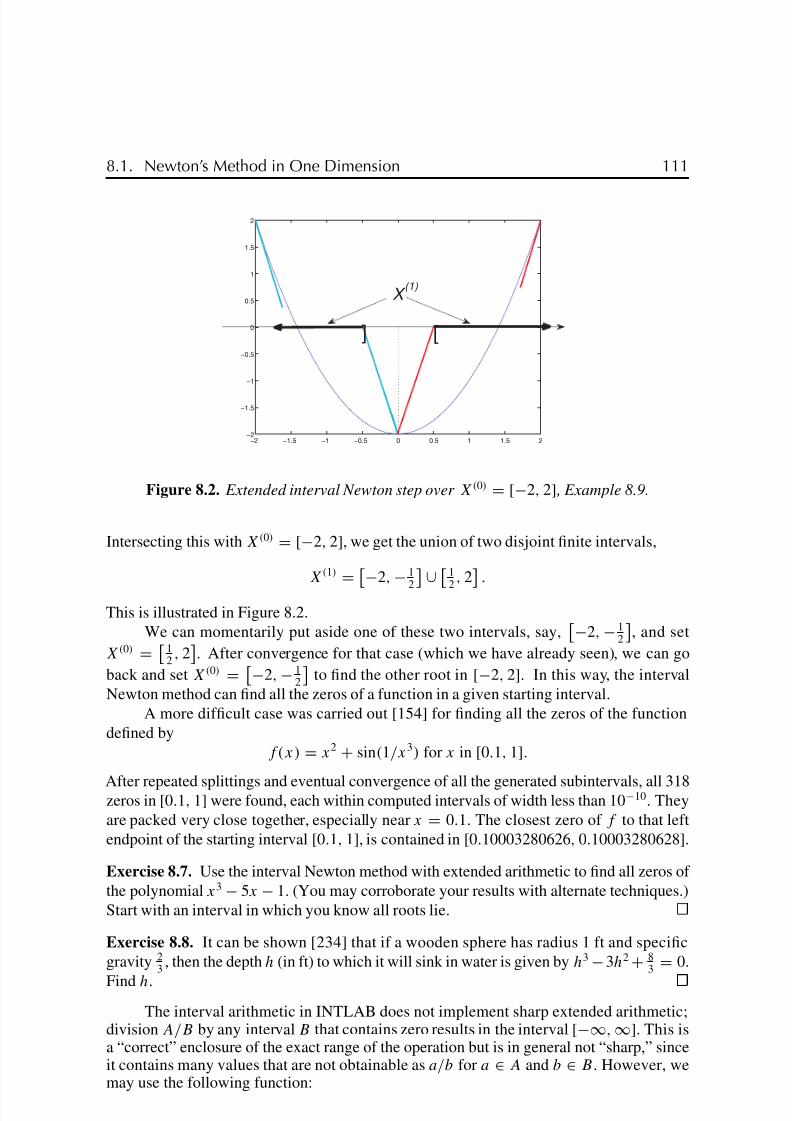
8/6/2019 Moore 1966
http://slidepdf.com/reader/full/moore-1966 122/234
8.1. Newton’s Method in One Dimension 111
−2 −1.5 −1 −0.5 0 0.5 1 1.5 2−2
−1.5
−1
−0.5
0
0.5
1
1.5
2
]
X
[
(1)
Figure 8.2. Extended interval Newton step over X(0) = [−2, 2] , Example 8.9.
Intersecting this with X(0) = [−2, 2], we get the union of two disjoint finite intervals,
X(1) =
−2, − 1
2
∪
1
2
, 2.
This is illustrated in Figure 8.2.
We can momentarily put aside one of these two intervals, say,
−2, − 12
, and set
X(0) =
12, 2
. After convergence for that case (which we have already seen), we can go
back and set X(0) =
−2, − 12
to find the other root in [−2, 2]. In this way, the interval
Newton method can find all the zeros of a function in a given starting interval.
A more difficult case was carried out [154] for finding all the zeros of the function
defined by
f(x) = x2 + sin(1/x3) for x in [0.1, 1].
After repeated splittings and eventual convergence of all the generated subintervals, all 318zeros in [0.1, 1] were found, each within computed intervals of width less than 10−10. They
are packed very close together, especially near x = 0.1. The closest zero of f to that left
endpoint of the starting interval [0.1, 1], is contained in [0.10003280626, 0.10003280628].
Exercise 8.7. Use the interval Newton method with extended arithmetic to find all zeros of
the polynomial x3 − 5x − 1. (You may corroborate your results with alternate techniques.)
Start with an interval in which you know all roots lie.
Exercise 8.8. It can be shown [234] that if a wooden sphere has radius 1 ft and specific
gravity 23
, then the depth h (in ft) to which it will sink in water is given by h3 − 3h2 + 83
= 0.
Find h.
The interval arithmetic in INTLAB does not implement sharp extended arithmetic;division A/B by any interval B that contains zero results in the interval [−∞, ∞]. This isa “correct” enclosure of the exact range of the operation but is in general not “sharp,” sinceit contains many values that are not obtainable as a/b for a ∈ A and b ∈ B. However, wemay use the following function:

8/6/2019 Moore 1966
http://slidepdf.com/reader/full/moore-1966 123/234

8/6/2019 Moore 1966
http://slidepdf.com/reader/full/moore-1966 124/234
8.1. Newton’s Method in One Dimension 113
In case we wish to find intervals containing the roots of a rational function f which
has coefficients known only to lie in certain intervals, we can take an interval extension F
which evaluates the range of values of f over the intervals of coefficients and use the more
general form
N(X) = m(X) − F(m(X))
F (X)(8.10)
for the Newton iteration function N(X).
Example 8.3. To find the roots of f(x) = x2 −c that lie in the interval [1, 2], for c ∈ [2, 3],
we can put
F(X) = X2 − [2, 3], F (X) = 2X, X0 = [1, 2],
and find N(X0) ⊆ [1.39, 1.76]. After one application of X(k+1) = N (X(k) ) ∩ X(k) , we have
{x : x2 − c = 0, c ∈ [2, 3] }∩ [1, 2] = [√
2,√
3] ⊆ [1.39, 1.76].
A fundamental distinction between the interval Newton method and the ordinary
Newton method is that the former uses computation with sets instead of computation with
points. Again, this permits us to find all the zeros of a function in a given starting interval.
Whereas the ordinary Newton method is prone to erratic behavior, the interval version
practically always converges. The difference in performance of the two methods can be
dramatic, and the interested reader is referred to Moore [152] for specific examples.
Exercise 8.11. The current I (mA) flowing in a diode circuit satisfies the equation 1 − I −0.0052 ln(109I ) = 0. Solve by the Newton method.
Exercise 8.12. The odd-numbered transverse electric modes of a glass slab waveguide have
permitted incidence angles θi given by [83],
tan
3
2π cos θi
=
sin2 θi − (9/4)−1
cos θi
.
Find all solutions θi that lie in the interval
π8
, π2
. (Be sure to choose starting intervals in
such a way that singularities are avoided.)
Notes
1. Extended interval arithmetic involving reciprocation or division by intervals that con-
tain zero has been the subject of much discussion and some controversy among experts
in interval computation. In particular, various systems have been devised for doing
computations on objects in which the system is closed under division by intervals
that contain zero. The first such work, still widely referenced and the basis of what
followed, is “Kahan arithmetic” [89]; the extended reciprocation defined here canbe considered to contain elements of Kahan arithmetic. The extended reciprocation
defined here serves well in the context of our univariate interval Newton algorithm.
However, there are contexts when it is useful to represent both semi-infinite intervals
resulting from the division as a single object, continuing to do nonstop, exception-
free arithmetic on these objects. In such arithmetics, there are issues of efficiency

8/6/2019 Moore 1966
http://slidepdf.com/reader/full/moore-1966 125/234
114 Chapter 8. Interval Newton Methods
of the operations when using standards such as the IEEE 745 standard for binary
floating point arithmetic, as well as issues of sharpness in enclosing exact ranges.
There are also issues of consistency and mathematical elegance. For instance, some
analyses suggest that it is preferable to have a system where, when c = 0 < d , the
set {−∞} ∪ [1/d, ∞] is returned instead of [1/d, ∞]. In such arithmetics, cases 1
and 3 of the reciprocation described above are limiting cases of case 2. A recent
work discussing this is [194]. In this work, a consistent mathematical system, Cset
arithmetic, is developed. The Cset , or “containment set” of an arithmetic expression
of n variables at a point in Rn is the set of all limits of the expression as the variables
in the expression tend to the point, and the Cset evaluation of a set or interval vector isthe union of the Csets of the points in the set. The interval evaluation of an expression
over an interval vector is then defined to be an enclosure of the Cset of the expression
over that interval vector.
Cset arithmetic is compelling from the points of view of simplicity and connections
with classical mathematical analysis. It also provides an unambiguous theoretical
guide about how the arithmetic operations and function definitions (exponentials,
trigonometric functions, etc.) should be extended.
2. The representations in function xreciprocal are presently subject to discussion
as part of an effort to standardize interval arithmetic, and the ultimate standardized
representation may differ from that seen in xreciprocal. For example, some view
1/0astheset [−∞, −∞]∪[∞, ∞], rather than the empty set; furthermore, ultimately,
the empty set might be represented by something other than [NaN,NaN].
3. A related controversial issue is whether the underlying set is the set of real numbers
or the set of extended real numbers, including −∞ and ∞. As an example of the
difference, consider applying the interval Newton method to the function f(x) =
sin(πx)/π with starting interval X = [−2.5, 2.5], so m(X) = 0, while the exact
range of f over X is [−1, 1]. Thus, the iteration (8.10) becomes
N(X) = 0 −0
[−1, 1] .
If we take the underlying model to be the set of real numbers but interpret 0/0
according to Cset theory to be the set of all limits of x/y as x → 0 and y → 0, then
we obtain 0/0 = (−∞, ∞), so N(X) = (−∞, ∞), and N(X) contains all solutions
of f(x) = 0 in X. (The solutions are x = −2, −1, 0, 1, and 2.) On the other hand,
suppose we write N(X) as
N(X) = m(X) − F(m(X)) ·1
F (X).
Assuming the underlying model is the set of real numbers, and not the extended reals,we have 1/F (X) = 0 · (−∞, ∞) = 0, and N(X) = [0, 0]. Thus, in this case, N(X)
does not contain all solutions to f(x) = 0 that are in X, that is, Theorem 8.1 is not
true with this extension of interval arithmetic. However, these operational definitions
of 0/[−1, 1] and 0 · (−∞, ∞) are implemented in many currently available and
proposed systems for doing interval arithmetic.

8/6/2019 Moore 1966
http://slidepdf.com/reader/full/moore-1966 126/234

8/6/2019 Moore 1966
http://slidepdf.com/reader/full/moore-1966 127/234
116 Chapter 8. Interval Newton Methods
8.2 The Krawczyk Method
In this and the following sections, we consider finite systems of nonlinear equations
f 1(x1, . . . , xn) = 0,
... (8.11)
f n(x1, . . . , xn) = 0,
which we may write in vector notation as
f(x) = 0. (8.12)
In this section, we consider the Krawczyk method (first introduced for linear systems
as (7.7)), while in section 8.4 we consider a somewhat more straightforward generalization
of the univariate interval Newton method. Each approach has its own advantages, and both
are used in practice.
We can consider two cases: (1) the functions f i are exactly representable real-valued
functions, or (2) the functions f i have coefficients known only to lie in certain intervals.
We will discuss case (1) first and extend the results to case (2).
Suppose that f in (8.12) is continuously differentiable in an open domainD. Suppose
that we can compute inclusion isotonic interval extensions F and F for f and f , defined
on interval vectors X ⊆ D. We have the following computational test for the existence of
a solution [119, 150].
Theorem 8.2. Let Y be a nonsingular real matrix approximating the inverse of the real
Jacobian matrix F (m(X)) with elements F (m(X))ij = ∂f i(x)/∂xj at x = m(X). Let y
be a real vector contained in the interval vector X ⊆ D. Define K(X) by
K(X) = y − Yf(y)+ {I − YF (X)}(X − y). (8.13)
If K(X) ⊆ X, then (8.12) has a solution in X. It is also in K(X).
An early work containing the proof of this theorem is [150]. The proof is based on
a generalization of the Brouwer fixed-point theorem, or a specific instance of the Schauder
fixed-point theorem. Namely, if X is a closed convex subset of Rn, and g maps X into itself,
then g has a fixed point x∗, x∗ = g(x∗), x∗ ∈ X.
Proof (of Theorem 8.2). Define g(y) = y−Yf(y). Then, since Y is nonsingular, g(y) = y
if and only if f(y) = 0. Thus, if there exists an x ∈ X such that g(x) = x, that is, if there
is a fixed point of g in x, then there is a solution to f(x) = 0 in x. However, if by g(y) we
mean the Jacobian matrix of g at y, then
g
(y) = I − Yf
(y).
Therefore, the mean value extension (see (6.25)) of g over X about the point y ∈ X is
simply34
y − Yf(y) + {I − YF (X)}(X − y) = K(X).
34Here, we have (6.25) for each component of f .
8/6/2019 Moore 1966
http://slidepdf.com/reader/full/moore-1966 128/234
8.2. The Krawczyk Method 117
Thus, K(X) must contain the range of g over X, that is, g(X) ⊆ K(X). Thus, if K(X) ⊆ X,
then g(X) ⊆ X, the hypotheses of the Schauder fixed-point theorem hold, so g has a fixed
point in X, so f(x) = 0 has a solution in X.
If the interval vector X = (X1, . . . , Xn) is an n-cube so that w(Xi ) = w(X) for
i = 1, . . . , n, and if we choose y = m(X), then K(X) lies in the interior of X if
K(X) − m(X) < w(X)/2. (8.14)
Thus, for an n-cube X, (8.14) is sufficient for the existence of a solution to (8.12) in X. The
same condition (8.14), which can be verified computationally by evaluating K(X), is also
sufficient to guarantee convergence of the interval Krawczyk method.
Theorem 8.3. Let X be an n-cube, y = m(X), and Y a nonsingular real matrix. Suppose
(8.14) is satisfied. Put X(0) = X, Y (0) = Y and consider an arbitrary real vector x(0) in X(0).
Then the system (8.11) has a unique solution in X, and the following algorithm converges
to the solution [150, 151]:
X(k+1) = X(k) ∩ K(X(k)) (k = 1, 2, . . . ) , (8.15)
whereK(X(k)) = y(k) − Y (k) f (y(k) ) + {I − Y (k)F (X(k) )}Z(k)
and
y(k) = m(X(k) ), Z(k) = X(k) − m(y(k)),
and where Y (k) is chosen as
Y (k) =
Y, an approximation to [m(F (X(k)))]−1
if
I − Y F (X(k) )
≤
I − Y (k−1)F (X(k−1))
,
Y
(k−1)
otherwise.
Example 8.4. Consider the system of equations
f 1(x1, x2) = x21 + x2
2 − 1 = 0,
f 2(x1, x2) = x1 − x22 = 0. (8.16)
For f we have the Jacobian matrix
f (x) = 2x1 2x2
1 −2x2 . (8.17)
For the interval extensions F and F , we can take the natural interval extensions of the corre-
sponding real rational functions, simply evaluating (8.16) and (8.17) in interval arithmetic:
F 1(X) = X21 + X2
2 − 1,
F 2(X) = X1 − X22 ,
and F (X) =
2X1 2X2
1 −2X2
.

8/6/2019 Moore 1966
http://slidepdf.com/reader/full/moore-1966 129/234
118 Chapter 8. Interval Newton Methods
Suppose we decide to try X = ([0.5, 0.8], [0.6, 0.9])T . Then, we have
m(F (X)) =
m([1, 1.6]) m([1.2, 1.8])
m([1, 1]) m([−1.8,−1.2])
=
1.3 1.5
1 −1.5
.
As an approximate inverse of this matrix, we will take
Y =
0.43 0.43
0.29 −0.37
. (8.18)
Putting y = (0.65, 0.75)
T
= m(X), we find from (8.13) for the 2-cube X,
K(X) ⊆ ([0.559, 0.68], [0.74, 0.84])T .
Since K(X) − m(X) = 0.091 < w(X)/2 = .15, the hypotheses for Theorem 8.3 are
satisfied. The iterative method (8.15) converges to a solution of (8.16) using Y given
by (8.18) from X(0) = ([0.5, 0.8], [0.6, 0.9])T . It produces a nested sequence of interval
vectors containing the solution, and using IA converges in a finite number of steps to an
interval vector containing a solution of (8.16).
It can be shown [159] that the widths of the containing interval vectors converge
quadratically to zero if F
(X) is a Lipschitz extension of f
(x).
INTLAB Implementation
The Krawczyk method can be implemented in INTLAB with the following m-file:
function [KX] = Krawczyk_step(X,y,f)
% [KX] = Krawczyk_step(X,y,f,fprime) returns the image of X
% from a step of the Krawczyk method, with base point y, where
% the function is programmed in the function whose name is in
% the string f. There is no need to program the Jacobian matrix,
% since the "gradient" automatic differentiation toolbox,% distributed with INTLAB, is used. It is the user’s
% responsibility to ensure that X is an interval column vector,
% that y is a non-interval column vector contained in X, and
% that f is the desired function in an "m" file that returns
% a column vector.
% First compute f(y) using interval arithmetic to bound
% roundoff error --
n=length(X);
iy = midrad(y,0);
fy = feval(f,iy);
% Now compute F’(X) and the preconditioning matrix Y --
Xg = gradientinit(X);
FXg = feval(f,Xg);
Y = inv(mid(FXg.dx));

8/6/2019 Moore 1966
http://slidepdf.com/reader/full/moore-1966 130/234

8/6/2019 Moore 1966
http://slidepdf.com/reader/full/moore-1966 131/234
8/6/2019 Moore 1966
http://slidepdf.com/reader/full/moore-1966 132/234
8.3. Safe Starting Intervals 121
the sequence of interval vectors generated by (8.15), starting with X(0) = X, Y (0) = Y , is a
nested sequence and converges in a finite number of steps (using IA) to an interval vector
containing all the solutions to (8.11) in X for any choice of the real coefficients from the
given interval coefficients. Thus we can compute bounds on the set of possible solutions
in X.
8.3 Safe Starting Intervals
A safe starting interval for the interval Newton method is an X(0) from which the method
(8.15) converges to a solution of a given nonlinear system of the form (8.11) or (8.12). FromTheorem 8.3, X(0) is a safe starting interval if (8.14) holds; equivalently if K(X(0)) ⊂ X(0),
that is, if K(X(0)) is contained in the interior of X(0),
K(X(0)) ⊂ X(0) =⇒ a solution is in K(X(0)). (8.19)
From Theorem 8.2, with K(X) defined by (8.13), if K(X) ⊆ X, there is a solution
in X, and it is also in K(X), so there is a solution in the intersection K(X) ∩ X. It follows
that if K(X) ∩ X is empty, there is no solution in X:
K(X)
∩X
= ∅ =⇒no solution in X. (8.20)
In searching within a region B of interest, where we would like to find solutions, we
can delete any part of B for which (8.20) holds. Furthermore, the extended definition of
interval division discussed following Exercise 8.3, which splits an interval and produces a
gap containing no solutions, can be extended to systems of nonlinear equations.
Example 8.5. We reconsider Exercise 8.12 to illustrate how we can find safe starting
intervals. We are interested in finding all solutions that lie in the interval [π8, π
2] to the
equation
tan 3
2
π cos θi =
sin2 θi − (9/4)−1
cos θi
.
We can rewrite the equation in the form f(x) = 0, using x instead of θi , where
f(x) = cos(x) tan
32π cos x
−(sin x)2 − 4
9.
The problem presents the interesting challenge that f(x) is not defined on all of the interval
of interestπ8, π
2
.
We can find the expression for
K(X) = y − Yf(y)+ {I − YF (X)}(X − y)
for this example as follows. For the derivative of f (x), we find that
f (x) = − tan
32π cos x
(sin x) − 3
2π
sin x
cos2
32π cos x
(cos x)
− 3sin x√
5 − 9cos2 xcos x. (8.21)
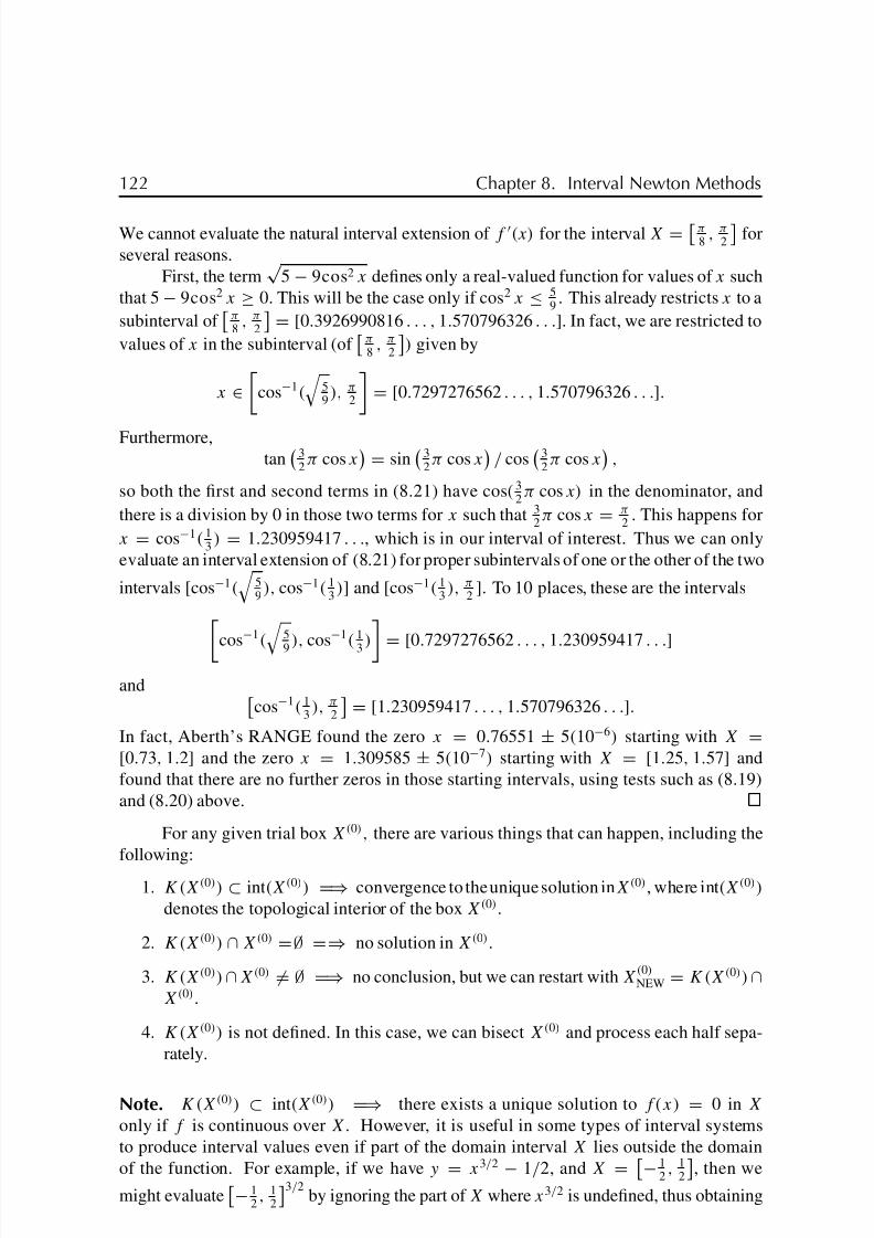
8/6/2019 Moore 1966
http://slidepdf.com/reader/full/moore-1966 133/234
122 Chapter 8. Interval Newton Methods
We cannot evaluate the natural interval extension of f (x) for the interval X = π8, π
2
for
several reasons.
First, the term√
5 − 9cos2 x defines only a real-valued function for values of x such
that 5 − 9cos2 x ≥ 0. This will be the case only if cos2 x ≤ 59
. This already restricts x to a
subinterval of π8, π
2
= [0.3926990816 . . . , 1.570796326 . . .]. In fact, we are restricted to
values of x in the subinterval (of π8, π
2
) given by
x ∈
cos−1(
59), π
2
= [0.7297276562 . . . , 1.570796326 . . .].
Furthermore,tan
32π cos x
= sin
32π cos x
/ cos
32π cos x
,
so both the first and second terms in (8.21) have cos( 32π cos x) in the denominator, and
there is a division by 0 in those two terms for x such that 32π cos x = π
2. This happens for
x = cos−1( 13) = 1.230959417 . . ., which is in our interval of interest. Thus we can only
evaluate an interval extension of (8.21) for proper subintervals of one or the other of the two
intervals [cos−1(
59), cos−1( 1
3)] and [cos−1( 1
3), π
2]. To 10 places, these are the intervals
cos−1( 5
9), cos−1( 1
3) = [
0.7297276562 . . . , 1.230959417 . . .]
and cos−1( 1
3), π
2
= [1.230959417 . . . , 1.570796326 . . .].In fact, Aberth’s RANGE found the zero x = 0.76551 ± 5(10−6) starting with X =[0.73, 1.2] and the zero x = 1.309585 ± 5(10−7) starting with X = [1.25, 1.57] and
found that there are no further zeros in those starting intervals, using tests such as (8.19)
and (8.20) above.
For any given trial box X(0), there are various things that can happen, including the
following:
1. K(X(0)) ⊂ int(X(0)) =⇒ convergence to the unique solution inX(0), where int(X(0))
denotes the topological interior of the box X(0).
2. K(X(0)) ∩ X(0) =∅ =⇒ no solution in X(0).
3. K(X(0))∩X(0) = ∅ =⇒ no conclusion, but we can restart with X(0)NEW = K(X(0))∩
X(0).
4. K(X(0)) is not defined. In this case, we can bisect X(0) and process each half sepa-
rately.
Note. K(X(0)) ⊂ int(X(0)) =⇒ there exists a unique solution to f(x) = 0 in X
only if f is continuous over X. However, it is useful in some types of interval systems
to produce interval values even if part of the domain interval X lies outside the domain
of the function. For example, if we have y = x3/2 − 1/2, and X = − 12, 1
2
, then we
might evaluate− 1
2, 1
2
3/2by ignoring the part of X where x3/2 is undefined, thus obtaining
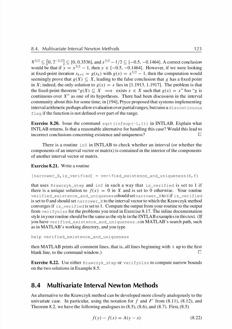
8/6/2019 Moore 1966
http://slidepdf.com/reader/full/moore-1966 134/234
8.4. Multivariate Interval Newton Methods 123
X3/2 ⊆
0, 2−3/2
⊆ [0, 0.3536], and x3/2 − 1/2 ⊆ [−0.5, −0.1464]. A correct conclusion
would be that if y = x3/2 − 1, then y ∈ [−0.5, −0.1464]. However, if we were looking
at fixed-point iteration xk+1 = g(xk) with g(x) = x3/2 − 1, then the computation would
seemingly prove that g(X) ⊆ X, leading to the false conclusion that g has a fixed point
in X; indeed, the only solution to g(x) = x lies in [1.1913, 1.1917]. The problem is that
the fixed-point theorem “g(X) ⊆ X =⇒ exists x ∈ X such that g(x) = x” has “g is
continuous over X” as one of its hypotheses. There had been discussion in the interval
community about this for some time; in [194], Pryce proposed that systems implementing
interval arithmetic perhaps allow evaluation over partial ranges, but raise a discontinuous
flag if the function is not defined over part of the range.
Exercise 8.20. Issue the command sqrt(infsup(-1,1)) in INTLAB. Explain what
INTLAB returns. Is that a reasonable alternative for handling this case? Would this lead to
incorrect conclusions concerning existence and uniqueness?
There is a routine in0 in INTLAB to check whether an interval (or whether the
components of an interval vector or matrix) is contained in the interior of the components
of another interval vector or matrix.
Exercise 8.21. Write a routine
[narrower_X,is_verified] = verified_existence_and_uniqueness(X,f)
that uses Krawczyk_step and in0 in such a way that is_verified is set to 1 if there is a unique solution to f(x) = 0 in X and is set to 0 otherwise. Your routineverified_existence_and_uniqueness should set narrower_X to X if is_verified
is set to 0 and should set narrower_X to the interval vector to which the Krawczyk methodconverges if is_verified is set to 1. Compare the output from your routine to the outputfrom verifynlss for the problems you tried in Exercise 8.17. The inline documentationstyle in your routine should be the same as the style in the INTLAB examples in this text. (If you have verified_existence_and_uniqueness.m in MATLAB’s search path, suchas in MATLAB’s working directory, and you type
help verified_existence_and_uniqueness
then MATLAB prints all comment lines, that is, all lines beginning with % up to the first
blank line, to the command window.)
Exercise 8.22. Use either Krawczyk_step or verifynlss to compute narrow bounds
on the two solutions in Example 8.5.
8.4 Multivariate Interval Newton Methods
An alternative to the Krawczyk method can be developed more closely analogously to the
univariate case. In particular, using the notation for f and F from (8.11), (8.12), and
Theorem 8.2, we have the following analogues to (8.5), (8.6), and (8.7). First, (8.5)
f(y) − f(x) = A(y − x) (8.22)

8/6/2019 Moore 1966
http://slidepdf.com/reader/full/moore-1966 135/234
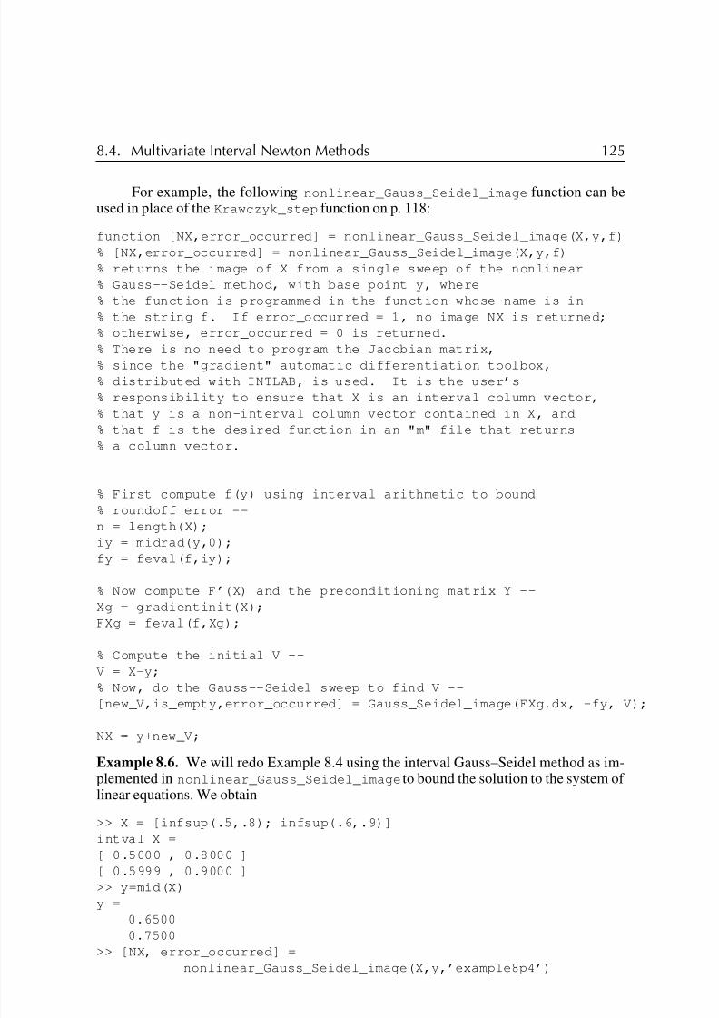
8/6/2019 Moore 1966
http://slidepdf.com/reader/full/moore-1966 136/234

8/6/2019 Moore 1966
http://slidepdf.com/reader/full/moore-1966 137/234
126 Chapter 8. Interval Newton Methods
intval NX =
[ 0.5687 , 0.6588 ]
[ 0.7702 , 0.8130 ]
error_occurred = 0
.
.
.
intval X =
[ 0.6172 , 0.6179 ]
[ 0.7848 , 0.7853 ]
>> [NX, error_occurred] =nonlinear_Gauss_Seidel_image(X,y,’example8p4’)
intval NX =
[ 0.6175 , 0.6176 ]
[ 0.7850 , 0.7851 ]
error_occurred = 0
Observe that the image after the first iteration is contained in the corresponding image afterthe first iteration of the Krawczyk method. This is true in general; the result occurs in [167](and possibly earlier). For this example, this is due to intrinsic mathematical properties of the Krawczyk method and the Gauss–Seidel method, not to the fact that the matrix Y in(8.18) is only an approximation. To see this, we can redo the computation with the loose
approximation (8.18):
>> X = [infsup(.5,.8); infsup(.6,.9)]
intval X =
[ 0.5000 , 0.8000 ]
[ 0.5999 , 0.9000 ]
>> y=mid(X)
y =
0.6500
0.7500
>> fprimex = [2*X(1) 2*X(2); 1 -2*X(2)]
intval fprimex =
[ 1.0000 , 1.6000] [ 1.1999, 1.8000 ]
[ 1.0000 , 1.0000] [ -1.8000, -1.1999 ]
>> fy = [y(1)ˆ2 + y(2)ˆ2-1;y(1)-y(2)ˆ2]
fy =
-0.0150
0.0875
>> y = midrad(y,0)
intval y =
[ 0.6499 , 0.6501 ]
[ 0.7499 , 0.7501 ]
> > V = X - y
intval V =
[ -0.1501 , 0.1500 ]
[ -0.1501 , 0.1500 ]
>> Y = [.43 .43; .29 -.37]
Y =
0.4300 0.4300
0.2900 -0.3700

8/6/2019 Moore 1966
http://slidepdf.com/reader/full/moore-1966 138/234
8.5. Concluding Remarks 127
>> [new_V_1, V12, there_are_2, num, denom] ...
= gauss_seidel_step(1,Y(1,:),fprimex, -fy, V)
intval new_V_1 = [ -0.0813 , 0.0088 ]
intval V12 = [ -0.1501 , 0.1500 ]
there_are_2 = 0
intval num = [ -0.0699 , 0.0076 ]
intval denom = [ 0.8599 , 1.1181 ]
>> new_X(1) = y(1)+new_V_1
intval new_X = [ 0.5687 , 0.6588 ]
Note We have stated the multidimensional interval Newton method somewhat more gen-
erally than the univariate one. In the univariate case, we fixed the base point y to be the
midpoint of X, but here, we left y arbitrary other than y ∈ X. In fact, the only requirement
for the univariate case is also y ∈ X, and there may be some advantages to choosing y other
than m(X).
8.5 Concluding Remarks
See Hansen and Walster [57] (especially their Chapters 9 and 11) for a thorough discussion
of interval Newton methods for nonlinear equations and nonlinear systems of equations.A treatment of the theory underlying the Krawczyk operator, the interval Gauss–Seidel
operator, and other aspects of interval techniques for linear and nonlinear systems appears
in [167].
It is possible to use a slope matrix (see p. 72) instead of a componentwise extension
to the Jacobian matrix in the interval Newton method. In [257], Shen and Wolfe study slope
enclosures and show that, in using them in the Krawczyk method, the method has higher
existence-proving power than the Newton–Kantorovich theorem.36 However, if slopes are
used in interval Newton methods, uniqueness is lost. In [219], Rump discusses this and
explains an efficient two-stage method whereby slopes can be used to prove both existence
and uniqueness.A number of experts in interval computations have produced software that automati-
cally finds all solutions, with mathematical rigor, to systems of nonlinear equations. Some
of our work, publicly available, is GlobSol. GlobSol implements a branch-and-bound
method in combination with computational existence and uniqueness based on a multivari-
ate interval Newton method to find all global optimizers of unconstrained or constrained
optimization problems or (with configuration variable NONLINEAR_SYSTEM set to .TRUE.)
all solutions to nonlinear systems of equations within a particular box. A brief description of
the history and capabilities of GlobSol can be found in [104], while an in-depth description
of some of the techniques in GlobSol, along with details concerning a very early version
of GlobSol (which was called intopt_90), can be found in [97]. The system of equationsor optimization problem is provided to GlobSol in the form of a Fortran 90 program. A
self-contained, easily installed version of GlobSol (distributed with a copy of the GNU
Fortran 95 compiler) for MS Windows is available.
36One place where this theorem is stated is [188, p. 421]. Interestingly, the hypotheses of the Newton–
Kantorovich theorem can be verified using interval arithmetic.

8/6/2019 Moore 1966
http://slidepdf.com/reader/full/moore-1966 139/234
128 Chapter 8. Interval Newton Methods
Interval versions of Newton’s method in Banach spaces are presented in Moore and
Cloud [156].
While the previous two chapters dealt with linear and nonlinear algebra, the next
chapter will use interval evaluations to bound error terms, for numerical integration with
verified error bounds.

8/6/2019 Moore 1966
http://slidepdf.com/reader/full/moore-1966 140/234
Chapter 9
Integration of IntervalFunctions
In this chapter we introduce the interval integral
[a,b]
F(t)dt
and use it to compute enclosures for the definite integrals of real-valued functions. We
also revisit the subject of automatic differentiation, whose origins date to the appearance
of modern computers [92], which appeared in the context of interval analysis in [157],
and which is an extensive subject in its own right [21, 54, 200]. Finally, we outline some
relationships between interval integration and the other, more familiar types of integration
(Riemann, Lebesgue, etc.).
9.1 Definition and Properties of the Integral
Let us begin with a real-valued continuous function f . We typically denote the ordinarydefinite integral
ba
f(t)dt by either
[a,b]
f(t)dt or
X
f(t)dt .
where X = [a, b].
Lemma 9.1. If f is continuous in X = [a, b], then
X
f(t)dt ∈ f (X)w(X). (9.1)
Proof. According to the mean value theorem for integrals, we can write
[a,b]
f(t)dt = f (s)(b − a) for some s ∈ [a, b]. (9.2)
But f(s) ∈ f(X), so the lemma follows.
129

8/6/2019 Moore 1966
http://slidepdf.com/reader/full/moore-1966 141/234

8/6/2019 Moore 1966
http://slidepdf.com/reader/full/moore-1966 142/234
9.1. Definition and Properties of the Integral 131
Theorem 9.2. [a,b]
f ( t ) d t =∞
N =1 S N (F ; [a, b]) = limN →∞
S N (F ; [a, b]). (9.9)
Proof. By (9.7), inequality (9.4) becomes
w(S N ) ≤ L(b − a)2/N. (9.10)
Therefore, w(S N ) → 0 as N → ∞, with the value of the integral lying in every S N by
(9.3).
It follows from Lemma 6.5 that the sequence of intervals defined by
Y 1 = S 1, Y k+1 = S k+1 ∩ Y k (k = 1, 2, . . . )
is nested and converges to the value of the integral. We have finite convergence if IA is
used.
We can use Theorem 9.2 to define the integral of an interval-valued function of a
real variable t . However, we first note that, while F(t) must be real-valued for a Lipschitz
interval extension F , this is not true for all useful inclusion isotonic interval functions. The
interval polynomial enclosures discussed later have interval number coefficients. In such
cases, the width of F(t) may not be zero for real t .
Suppose that an interval-valued function with values F(X) is continuous and inclusion
isotonic for X ⊆ X0. If [a, b] ⊆ X0, the sums S N (F ; [a, b]) given in (9.8) are well defined.
For real arguments t (degenerate intervals [t, t ]), the values of F(t) may be real numbers
or intervals.
Definition 9.1. We define the interval integral [a,b]
F(t)d t =∞
N =1 S N (F ; [a, b]). (9.11)
It follows from the continuity of F that there are two continuous real-valued functions
F and F such that, for real t ,F(t) =
F(t),F(t)
.
Moreover, the integral defined by (9.11) is equivalent to [a,b]
F(t)d t =
[a,b]
F(t) dt ,
[a,b]
F(t)d t
. (9.12)
Example 9.1. Suppose 0 < a < b and let F(t) = A t k , where A =
A, A
and k is a
positive integer. By (9.12) we have
[a,b] F(t)d t =
[a,b] A t
k
dt ,
[a,b] A t
k
dt
=
A
bk+1 − ak+1
k + 1, A
bk+1 − ak+1
k + 1
= Abk+1 − ak+1
k + 1.
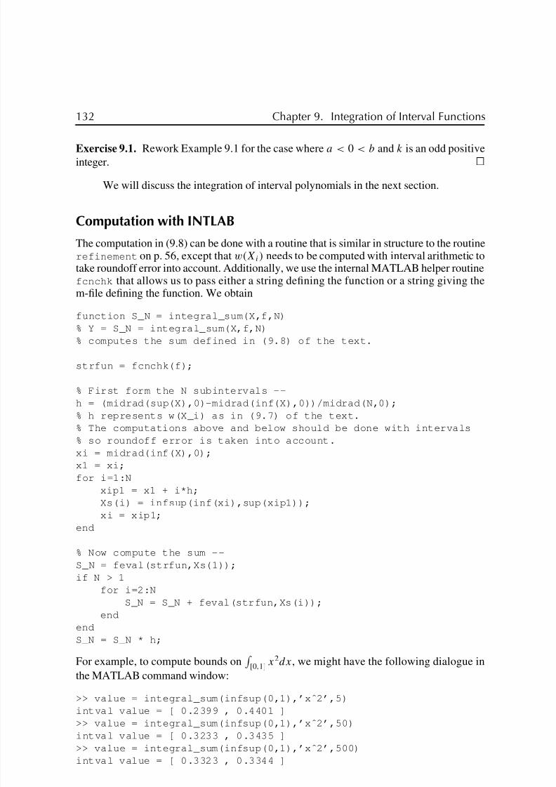
8/6/2019 Moore 1966
http://slidepdf.com/reader/full/moore-1966 143/234
8/6/2019 Moore 1966
http://slidepdf.com/reader/full/moore-1966 144/234
9.2. Integration of Polynomials 133
>> value = integral_sum(infsup(0,1),’xˆ2’,5000)
intval value = [ 0.3332 , 0.3335 ]
Just as Riemann sums are not the most efficient or accurate way to approximately
evaluate integrals using floating point arithmetic, (9.8) is not the most efficient or sharpest
way to obtain bounds on an interval integral. For instance, the call above to integral_sum
with N=5000 took a noticeable amount of time, in part because that execution of explicitly
programmed loops in MATLAB is much slower than in compiled languages. However,
efficient implementations of more sophisticated methods to get sharp bounds for the interval
integral exist. We will explain some of the more advanced techniques later in this chapter.
Exercise 9.2. Use integral_sum with various N to compute bounds on the following
integrals:
(a) the elliptic integral of the first kindF(k,φ) = φ
0(1−k2 sin2 t)−1/2 dt with parameters
φ = 2π and k = 0.5;
(b) the Fresnel sine integral f(x) = x
0sin(t 2) dt at x = 100.
Exercise 9.3. If you have Aberth’s RANGE software, repeat Exercise 9.2 using that soft-
ware.37
Inclusion Property
We end this section by stating one more property of the interval integral:
If F(t) ⊆ G(t) for all t ∈ [a, b], then
[a,b]
F(t)dt ⊆
[a,b]
G(t)dt. (9.13)
In other words, interval integration preserves inclusion.
Exercise 9.4. Prove (9.13).
9.2 Integration of Polynomials
Exercise 9.1 shows that care must be taken when integrating power-type functions having
interval coefficients. Here we will summarize the results for an interval polynomial of the
form
P(t) = A0 + A1t + · · · + Aq t q , (9.14)
where t is real and Ai = [Ai, Ai] for i = 0, 1, . . . , q. There are two cases:
Case 1. If a and b have the same sign, then
[a,b]
P(t)dt = A0(b − a) + · · · + Aq(bq+1 − aq+1)/(q + 1).
37See the web page for this book, www.siam.org/books/ot110.

8/6/2019 Moore 1966
http://slidepdf.com/reader/full/moore-1966 145/234
134 Chapter 9. Integration of Interval Functions
Case 2. If a < 0 < b, then [a,b]
P( t) d t = T 0 + T 1 + · · · + T q ,
where
T i =
Ai (bi+1 − ai+1)/(i + 1), i even,
(Ai bi+1 − Aai+1)/(i + 1) , (Ai bi+1 − Aai+1)/(i + 1)
, i odd.
Note that for “real” (degenerate interval) coefficients Ai , with Ai = Ai , both cases reduceto the usual formal integration of polynomials.
INTLAB Implementation
The following MATLAB function implements the above formulas:
function I = interval_poly_integral(X,A)
% I = interval_poly_integral(X,A) returns the interval integral
% over the interval X of the polynomial with interval coefficients
% given by A(1) + A(2) x + ... + A(q+1) xˆq, using the
% formulas given in Section 8.2 of the text by Moore, Kearfott,% and Cloud.
q = length(A)-1;
a = inf(X);
b = sup(X);
ia = midrad(a,0);
ib = midrad(b,0);
if ( (a >=0) & (b >=0) ) | ( (a <=0) & (b <=0) )
I = midrad(0,0);
for i=1:q+1;
I = I + A(i)*(ibˆi - iaˆi)/midrad(i,0);
endelse
I = midrad(0,0);
for i=1:q+1;
if mod(i,2)
T_i = A(i)*(ibˆi-iaˆi)/midrad(i,0);
else
lb = ( midrad(inf(A(i)),0) * ibˆi...
-midrad(sup(A(i)),0) * iaˆi )...
/ midrad(i,0)
ub = ( midrad(sup(A(i)),0) * ibˆi ...
-midrad(inf(A(i)),0) * iaˆi ) .../ midrad(i,0)
T_i = infsup(inf(lb),sup(ub));
end
I = I + T _ i ;
end
end

8/6/2019 Moore 1966
http://slidepdf.com/reader/full/moore-1966 146/234
9.3. Polynomial Enclosure, Automatic Differentiation 135
Exercise 9.5. Try interval_poly_integral to compute
[−1,1]
[1, 2]+ [−3, 4]x + [−0.5, 0.5]x2
dx.
Check the result by hand.
9.3 Polynomial Enclosure and Automatic Differentiation
The main goal of this chapter is to discuss the computation of enclosures for the values of definite integrals such as
[a,b]
f(t)dt .
Broadly speaking, the approach is to (1) enclose f(t) with a suitable interval function G(t)
and then (2) integrate G(t). We carry out this procedure in section 9.4. The present section is
devoted to step (1)—the definition and efficient computation of useful function enclosures.
Definition 9.2. Let T 0 be an interval and x a real-valued function of the real variable t , with
x(t) defined for all t ∈ T 0. An interval enclosure of x is an inclusion isotonic interval-valued
function X of an interval variable T , with X(T) defined for all T ⊆ T 0, having the property
that
x(t) ∈ X(t) for all t ∈ T 0. (9.15)
Hence, x(T) ⊆ X(T) for all T ⊆ T 0.
Example 9.2. Suppose x(t) satisfies a ≤ x(t) ≤ b for all t ∈ T 0. Then the constant interval
function X(T) ≡ [a, b] is an interval enclosure of x.
Note that X(t) in (9.15) is not necessarily real; it may be a nondegenerate interval
for each value of t . If X(t) = x(t) for all t ∈ T 0, then X is an inclusion isotonic interval
extension of x. This latter case will hold if X(t) takes the form of a polynomial in t with
interval coefficients, i.e., the form (9.14).
Definition 9.3. If X(t) in Definition 9.2 takes the form (9.14), it is called an interval
polynomial enclosure of x.
Example 9.3. Suppose x(t) is continuously differentiable on T 0 and that X(T ) is an in-
clusion isotonic interval extension of x (t). By the mean value theorem we have, for any
t 0 ∈ T 0,
x(t) = x(t 0)+ x (s)(t − t 0) for some s between t and t 0. (9.16)
It follows that X(T) = x(t 0)+X(T 0)(T − t 0) is an interval enclosure of x. The interval-
valued function X(t) of the real variable t is an interval polynomial enclosure of x. We
have
x(t) ∈ X(t) = x(t 0)+X(T 0)(t − t 0) for all t ∈ T 0. (9.17)

8/6/2019 Moore 1966
http://slidepdf.com/reader/full/moore-1966 147/234
136 Chapter 9. Integration of Interval Functions
We can extend the idea of (9.16) by working with Taylor expansions, for which we
introduce some notation. Suppose x(t) is analytic in t in some neighborhood of t 0. We
define
(x)0 = x(t 0),
(x)k =1
k!
d k x
dt k(t 0) (k = 1, 2, . . . ) . (9.18)
That is, (x)k is the kth Taylor coefficient in the expansion of x(t) about t = t 0:
x(t) =
∞
k=0
(x)k (t − t 0)k . (9.19)
For the finite Taylor expansion with Lagrange form of the remainder, we have
x(t) =
N −1
k=0
(x)k (t − t 0)k + (x)N (s)(t − t 0)N for some s ∈ [t 0, t ]. (9.20)
If RN is an interval enclosure of xN (s) so that
(x)N (s) ∈ RN ([t 0, t ]) for all s ∈ [t 0, t ],
for t within the radius of convergence of (9.19), we have
x(t) ∈
N −1
k=0
(x)k (t − t 0)k + RN ([t 0, t ])(t − t 0)N . (9.21)
The right-hand side is an enclosure for the Taylor series with remainder (9.20).
Example 9.4. If x(t) is analytic for t ∈ T 0, the interval polynomial
XN (t ) =
N −1
k=0
(x)k (t − t 0)
k
+ RN (T 0)(t − t 0)
N
(9.22)
is an enclosure of x. The values of XN (T ) for nondegenerate intervals T ⊆ T 0 are also
defined, and we have
x(t) ∈ XN (t ) ⊆ XN (T ) =
N −1
k=0
(x)k (T − t 0)k + RN (T 0)(T − t 0)N (9.23)
for all t ∈ T ⊆ T 0. As a specific application of (9.22), let x(t) = et and take t 0 = 0,
T 0 = [0, 1], N = 2. We have
et ∈ 1 + t + 12
[1, e] t 2 =
1 + t + 12
t 2 , 1 + t + e
2t 2
for all t ∈ [0, 1].
For a finite representation, which is still an interval polynomial enclosure, we can take
X(t) = 1 + t + [0.5, 1.359141] t 2. For a sharper enclosure, we can take N = 10 in (9.22)
to obtain
et ∈ X10(t ) = 1 + t + 1
2t 2 + · · · + 1
9!t 9 + 1
10![1, e] t 10.

8/6/2019 Moore 1966
http://slidepdf.com/reader/full/moore-1966 148/234
9.3. Polynomial Enclosure, Automatic Differentiation 137
Only the last coefficient is a nondegenerate interval. It is contained in the finitely represented
interval [0.27 · 10−6, 0.75 · 10−6]. We can enclose the real coefficients in narrow intervals
to obtain a finitely represented interval polynomial enclosure X(t) which contains X10(t)
for every t ∈ [0, 1]. Of course, X(t) also contains et for every t ∈ [0, 1].
Note Use of Taylor polynomials in this way is a heuristic that often, but not always,
reduces overestimation and excess width as we take polynomials and error terms of increas-
ingly higher order. For example, if high-order Taylor polynomials centered on t = 0 were
used to approximate et for |t | large and t negative, then the interval widths would increase as
higher-order polynomials were taken. This phenomenon is analogous to the cancelation er-
ror we would observe, were we to approximate such et with a high-order Taylor polynomial
with floating point arithmetic.
It remains to discuss how the Taylor coefficients (x)k can be evaluated efficiently.
An inefficient approach would be to use (9.18) to generate formulas for the (x)k in terms
of t and then evaluate them at t 0. Indeed, the expressions for the successive derivatives of
practical functions x typically become so involved that things can seem hopeless for all but
the smallest values of k. Fortunately, it is not necessary to generate explicit formulas for
the (x)k to obtain the values (x)k(t 0). The latter can be computed numerically using the
techniques of automatic differentiation.The approach amounts to differentiating computer subroutines (or function subpro-
grams). The result of differentiating a program is another program. When executed, the
derived program produces a value of the derivative of the function defined by the first pro-
gram. In fact, we can write a general-purpose program which, when applied to a function
defined by another program, will produce a Kth derivative program for general K for that
function. If we supply it with an integer K and argument values, it will produce values
of the derivatives (or Taylor coefficients) up to order K of the given function at the given
argument values. This can be carried out in machine arithmetic or in IA. Partial derivatives
can be obtained in a similar way. Early references on this are [147, 148, 157]; a somewhat
more recent one is [200], while a more recent, comprehensive overview in technical termsis [53].
We will now show how to compute the real and interval values (x)k and RN ([t 0, t ]).
The technique will apply to almost any quantity dependent on x that is computed with a
computer program. From (9.18) we find that x(t 0) = (x)1, so
(x)k =1
k((x)1)k−1. (9.24)
This relation is important, because if we have a function x(t) defined by a differential
equation, for instance,
x (t) = g(t, x(t)) with a given x(t 0),
then we can use
(x)k =1
k(g)k−1
8/6/2019 Moore 1966
http://slidepdf.com/reader/full/moore-1966 149/234
138 Chapter 9. Integration of Interval Functions
recursively to compute the Taylor coefficients for x(t) about t 0—provided, of course, that
we can handle g(t,x(t)). Similarly,
(x)k =2
k(k − 1)((x)2)k−2.
As far as the arithmetic operations are concerned, if u and v are analytic functions of
t in some neighborhood of t = t 0, then
(u + v)k = (u)k + (v)k,
(u − v)k = (u)k − (v)k,
(uv)k =
kj=0
(u)j (v)k−j ,
uv
k
=
1
(v)0
(u)k −
kj=1
(v)j
uv
k−j
.
(9.25)
Exercise 9.6. Derive a few of these formulas.
All the commonly used “elementary” functions satisfy rational differential equations.Any second-order differential equations that may occur can be rewritten as pairs of first-
order equations. With this and (9.24), we can derive recursion relations for the kth Taylor
coefficients of elementary functions of an arbitrary analytic function u(t). For example,38
(ua)k =
1
u
k−1j=0
a −
j (a + 1)
k
(u)k−j (u
a)j ,
(eu)k =
k−1j=0
1 −
j
k
(eu)j (u)k−j ,
(ln u)k =
1
u
(u)k −
k−1j=1
1 −
j
k
(u)j (ln u)k−j
,
(sin u)k =
1
k
k−1j=0
(j + 1)(cos u)k−1−j (u)j+1,
(cos u)k = −
1
k
k−1j=0
(j + 1)(sin u)k−1−j (u)j+1.
(9.26)
Similar relations are available for the hyperbolic functions, the Bessel functions, and various
other functions commonly used in applied mathematics.
Exercise 9.7. Show the following:
(a) If u(t) = constant, then (uv)k = u(v)k.
38In the relation for (ln u)k , the sum is deleted if k = 1.

8/6/2019 Moore 1966
http://slidepdf.com/reader/full/moore-1966 150/234
9.3. Polynomial Enclosure, Automatic Differentiation 139
(b) When u(t) = t , we have
(et )k =1
k(et )k−1 and the pair
(sin t)k =
1k(cos t)k−1,
(cos t)k = −1k(sin t)k−1.
The sine and cosine formulas should be computed together, even if only one is needed
directly. This will be illustrated in Example 9.6.
A general procedure for computing the Taylor coefficients of functions x(t) can be
programmed to operate as follows:
1. Represent x(t) (or x(t) or x (t) · · · ) by a finite list of binary or unary operations
(e.g., T 3 = T 1 + T 2, T 4 = eT 3 , etc.).
2. On a line-by-line basis, generate subprograms for Taylor coefficients for each item in
the list, using the recursion relation appropriate for the operation in that item.
3. Organize the subprograms and the data handling so that the derived program will
accept initial values for N, t 0,x(t 0) (and x (t 0), x (t 0) , . . . , if required); the derived
program will evaluate and store, in order, the first Taylor coefficients of each item in
the list, then the second Taylor coefficient of each item in the list (which may requiresome of the stored values of the first coefficients and initial data), etc., until the entire
array of coefficients has been computed; the process can be carried out either in real
computer arithmetic or in IA.
4. The list in step 1 can be generated from a subprogram description of x(t).
Example 9.5. Consider the function x(t) defined (when t 0 and x(t 0) are given) by the
differential equation
x (t) = x2+ t 2. (9.27)
For simplicity (to use the formula in (9.25) for multiplication, rather than the first formulain (9.26)), we write x2 as x · x and t 2 as t · t . (We would prefer (9.26) for sharpness in
interval evaluations.) We have
(T 1)0 = t · t,
(T 2)0 = (x)0 · (x)0,
(x)1 = T 1 + T 2.
(9.28)
Applying the third recursion in (9.25), we obtain
(T 1)k =
kj=0
(t)j (t)k−j ,
(T 2)k =
kj=0
(x)j (x)k−j ,
(x)k+1 = ((T 1)k + (T 2)k)/(k + 1).
(9.29)

8/6/2019 Moore 1966
http://slidepdf.com/reader/full/moore-1966 151/234
140 Chapter 9. Integration of Interval Functions
Since (t)1 = 1 and (t)j = 0 for j > 1, the straightforward application of the recursion
relations (9.29) could be modified to recognize that (T 1)k = 0 when k ≥ 3. Even without
any such simplification, the relations (9.29) suffice for the numerical evaluation of any
number of Taylor coefficients (x)k , k = 1, 2, . . ., for the function x(t). The total number
of arithmetic operations required to find (x)k for k = 1, . . . , N not taking into account
simplifications possible because of zero terms is (from (9.28) and (9.29)) N 2 + N − 1
additions, N 2 + N multiplications, and N − 1 divisions.
Exercise 9.8. Repeat Example 9.29 using T 1 = t 2 and T 2 = x2. Assuming t 0 = 1 and
x(t 0) = 0, use the recursions you so obtain to compute the first five Taylor coefficients for
x(t) expanded about t = 1.
The number of arithmetic operations to compute the kth Taylor coefficient of any func-
tion expressible as a finite combination of rational, elementary, and composition functions
grows at most linearly with k once the coefficients of lower orders have been obtained and
stored by the process described. Thus, the total number of arithmetic operations to obtain
the set of Taylor coefficients of orders 1, . . . , N grows no faster than cN 2 for some constant
c independent of N and depending only on the particular function in question.
Example 9.6. Consider
x(t) = e− sin t
ln(1+ t). (9.30)
We can represent x(t) by the list
T 1 = sin t,
T 2 = ln(1 + t),
T 3 = e−T 1 ,
T 4 = cos t,
x(t) = T 2 · T 3.
(9.31)
Applying the appropriate relations from (9.25) and (9.26) on a line-by-line basis, we obtain,
using (t)0 = t , (t)1 = 1, and (t)j = 0 for j > 1,
(T 1)k =1
k(T 4)k−1,
(T 2)k =1
1 + t
ak −
1 −
1
k
(T 2)k−1
, ak =
1, k = 1,
0, k > 1,
(T 3)k =
k−1
j=01 −
j
k (T 3)j (−T 1)k−j ,
(T 4)k = −1
k(T 1)k−1,
(x)k =
kj=0
(T 2)j (T 3)k−j . (9.32)

8/6/2019 Moore 1966
http://slidepdf.com/reader/full/moore-1966 152/234
9.4. Computing Enclosures for Integrals 141
We compute and store the following two-dimensional array of quantities proceeding down-
ward through the elements of a given column before continuing with the first element of the
next column to the right:
T 1 (T 1)1 (T 1)2 · · ·
T 2 (T 2)1 (T 2)2 · · ·
T 2 (T 2)1 (T 2)2 · · ·
T 4 (T 4)1 (T 4)2 · · ·
x (x)1 (x)2 · · ·
Again the total arithmetic computation required to find the Taylor coefficients of orders
1, . . . , N for x(t) defined by (9.30) at any value of t is of order N 2
(about32 N
2
additionsand multiplications). Note that the functions sin t , cos t , ln(1+t), e− sin t need to be evaluated
only once each, at the outset of the process.
We can bound the remainder term in (9.20) for this x(t) by using interval extensions
of sin t , cos t , ln(1 + t), and e−T 1 . Carrying out evaluations of those interval extensions
for the interval [t 0, t ] and following this with evaluations of the Taylor coefficients, using
(9.32) in interval arithmetic, we can obtain RN ([t 0, t ]) in (9.21).
Notes
1. Martin Berz, Kyoko Makino, and collaborators have provided an implementation of
computation of multivariate Taylor coefficients that is highly successful in applica-
tions; see the COSY web page.
2. In many instances, it is more efficient to arrange the computations in automatic dif-
ferentiation in a different order than has been presented here. This is particularly so
if just the function, gradient, and, perhaps, directional second-order derivatives are
needed. The computational scheme presented here is commonly called the forward
mode. To compute the value of gradient of a function of n variables, the forward mode
typically requires n times the amount of work required to compute the value of the
function itself. An alternative is thebackward mode, in which the intermediate results
in the computation are first computed and stored, then a system is solved to obtain thevalues. In contrast to the forward mode, computing the values of the function and the
gradient using the backward mode requires only a constant multiple (around 5) times
the amount of work required to compute just the value of the function but requires
storage that is proportional to the number of operations required to compute the func-
tion. The backward mode was perhaps first introduced by Speelpenning [235] and
has since been strongly advocated by Griewank [53], Christianson [36], and others.
The backward mode is explained in elementary terms in texts such as [3]. A compre-
hensive monograph including details of efficient implementation of both the forward
mode and backward mode is [53].
9.4 Computing Enclosures for Integrals
It follows from (9.13) that if G is an interval polynomial enclosure of f , then [a,b]
f ( t ) d t ∈
[a,b]
G(t)dt. (9.33)

8/6/2019 Moore 1966
http://slidepdf.com/reader/full/moore-1966 153/234
142 Chapter 9. Integration of Interval Functions
More generally, (9.33) holds if f is real-valued and G is interval-valued, continuous, and
inclusion isotonic, with f(t) ∈ G(t) for all t ∈ [a, b].
Example 9.7. Consider f(t) = 1/t and put F(X) = 1/X. From (9.5) we have
[1,2]
(1/t)dt ∈ (1/[1, 2]) =
12, 1. (9.34)
From (9.8), we have
S N =
N i=1
(1/(1 + [i − 1, i]/N))/N
=
N i=1
[1/(N + i), 1/(N + i − 1)].
Using three-digit IA we obtain
S ∗1 = [0.5, 1.0],
S ∗2 = [0.583, 0.834],
S
∗
3 = [0.617, 0.783],...
S ∗10 = [0.663, 0.722].
Exercise 9.9. Use the MATLAB function integral_sum on p. 132 from section 9.1 to
compute S 1 through S 10 in Example 9.7, using INTLAB’s internal interval arithmetic.
For the exact value of S N in Example 9.7, we have the actual widths w(S N ) =
1/N − 1/(2N) = 1/(2N), so the sequence Y ∗k+1S ∗k+1 ∩ Y ∗k with Y ∗1 = S ∗1 converges (using
three-digit IA) in no more than 500 steps to an interval of width no less than 0.001 containing
the exact value of the integral. This is slow convergence for such an easy integral; we willintroduce faster methods for bounding integrals in this section. First, however, an example
is needed to illustrate the application of (9.33) and (9.11).
Example 9.8. Suppose we wish to find upper and lower bounds on the integral
I =
1
0
e−t 2 dt. (9.35)
For the integrand in (9.35) we have the interval polynomial enclosure P defined by
e−t 2
∈ P(t) = 1 − t 2
+
1
2 t 4
− [0.0613, 0.1667] t 6
(9.36)
for all t ∈ [0, 1]. The interval coefficient [0.0613, 0.1667] bounds the range of values of 16e−s2
for all s ∈ [0, 1]. From (9.33) we find, for I in (9.35),
I ∈
[0,1]
P(t)dt. (9.37)

8/6/2019 Moore 1966
http://slidepdf.com/reader/full/moore-1966 154/234
9.4. Computing Enclosures for Integrals 143
It follows from (9.12) and (9.36) that
I ∈
[0,1]
P(t)dt =
1 − 13+ 1
10−
.16677
, 1 − 13+ 1
10−
.06137
⊆ [0.742, 0.758]. (9.38)
By using narrower interval polynomial enclosures, we can, as we shall see, compute arbi-
trarily sharp bounds on the exact value of integrals such as (9.35).
Using automatic differentiation, we can efficiently compute enclosures for integrals.
From (9.21) and (9.6) we have the following theorem for any positive integers K and N , if
a and b have the same sign.
Theorem 9.3. [a,b]
f(t)dt ∈
N i=1
K−1k=0
1
k + 1(f )k(Xi)w(Xi)
k+1
+1
K + 1(f )K(Xi)w(Xi)
K+1
(9.39)
for functions f with inclusion isotonic interval extensions of f and its first K derivatives.
This includes the class FCn(X0).
Proof. From the Lipschitz property of the interval extensions, there is a constant LK suchthat
w((f)K(Xi)) ≤ LKw(Xi) for all Xi ⊆ [a, b] ⊆ X0. (9.40)
Let us denote the right-hand side of (9.39) by I N,K . Since only the (f )K(Xi) con-
tribute anything to the width of I N,K , we have
w(I N,K ) = w
N i=1
1
K + 1(f )K(Xi)w(Xi)
K+1
=
1
K + 1
N i=1
w [(f )K(Xi)]w(Xi)K+1
≤LK
K + 1
N i=1
w(Xi)w(Xi)K+1 by (9.40)
=LK
K + 1
N i=1
w(Xi)K+2.
Hence,
w(I N,K ) ≤
LK
K + 1
N i=1
w(Xi)K+2
. (9.41)
For a uniform subdivision of [a, b], we have w(Xi) = (b − a)/N for i = 1, . . . , N , and
(9.41) becomes
w(I N,K ) ≤ CKhK+1, where CK =
LK
K + 1(b− a) and h =
b − a
N . (9.42)

8/6/2019 Moore 1966
http://slidepdf.com/reader/full/moore-1966 155/234
144 Chapter 9. Integration of Interval Functions
Thus, for fixed K, I N,K contains the exact value of the integral and has width no more than
some constant CK times the (K + 1)st power of the “step size” h.
Example 9.9. For (9.34), we can take LK = K + 1 (cf. Exercise 9.10), and hence CK = 1
for all K. Thus, I N ,K for the application of (9.39) to (9.34) is, for uniform subdivision, an
interval of width no more than (1/N)K+1 for any positive integers N and K. Furthermore,
we have
(f )k(Xi ) = (−1)k/Xk+1i , (f )K (Xi ) = (−1)K /XK+1
i ,
with
Xi = 1 + (i − 1)/N, w(Xi ) = 1/N, Xi = 1 + [i − 1, i]/N.To make the w(I N,K ) ≤ 0.001, we can take N ≥ 103/(K+1). The simpler method (9.8) with
width bounded by (9.10) corresponds to putting K = 0 in (9.39) and deleting the sum over
k. The following pairs of integers satisfy N ≥ 103/(K+1).
K N
0 1000
1 32
2 10
3 6
4 4
5 4
6 3
7 3
8 3
9 2
For K > 9 we still need N = 2.
Since the exact value of the integral is contained in I N,K for every pair of integers
N ≥ 1, K ≥ 0, we can intersect the intervals I N,K for any sequence of pairs of integers
{(N,K)} and obtain an interval which still contains the exact value of the integral. If wecarry out all the computations in I N,K using IA, then any sequence of such intersections
will converge in some finite number of steps to an interval containing the exact value of the
integral. We could fix N and take an increasing sequence of values of K, or fix K and take
an increasing sequence of values of N , for instance.
Exercise 9.10. Verify that we may take LK = K + 1 in Example 9.9.
Example 9.10. For (9.35) we can also apply (9.39) to compute I N,K for any N ≥ 1, K ≥ 0,
using the recursion formulas
(f )0(X) = e−X2
,(f )1(X) = −2X(f)0(X),
(f )k(X) = −(2/k)(X(f )k−1(X) + (f )k−2(X)) for n ≥ 2. (9.43)
For N = 2 and K = 6, using IA, we find I N,K = I 2,6 = [0.746, 0.748]. Compare with
(9.38).

8/6/2019 Moore 1966
http://slidepdf.com/reader/full/moore-1966 156/234
9.5. Further Remarks on Interval Integration 145
We can also apply (9.39) to more complicated functions in FC n(X0), e.g. x(t) in
(9.30) using the recursion relations (9.32) for the derivatives.
Note that, during the computation of I N,K using (9.39) in IA, we must also compute
the coefficients (f )k(Xi ) in IA to ensure that the computed interval value of I N,K contains
the value defined by (9.39).
9.5 Further Remarks on Interval Integration
A computer implementation of an interval integration routine typically finds the Taylor
coefficients automatically, generates the interval enclosure of the associated remainder term,and adaptively chooses intervals of expansion within the interval of integration, until the
entire integral is computed. If the data is given precisely, this can even be done to specified
accuracy. If there is uncertainty in the data itself, for instance, if all we know about α is an
interval that contains its value, we cannot expect to find a narrower interval containing the
integral than is allowed by the uncertainty in the data. In any case, an interval enclosure of
the integral still can be obtained.
Lang et al. [81, 129] as well as Krämer et al. [118] have successfully applied the
techniques we have been describing to adaptive Gaussian quadrature, for rigorously verified
enclosures of integrals.
We can also carry out interval integration over domains in more than one dimension,that is, we can compute multiple integrals. Let us briefly discuss interval integration over
a simplex. A nondegenerate simplex S d in Rd can be represented by
S d =
x =
d i=0
xi p(i) : 0 ≤ xi ≤ 1,
d i=0
xi ≤ 1
,
where {p(0), p(1), . . . , p(d)} is the set of d + 1 vertices. For d = 3, S 3 is a tetrahedron.
The barycentric coordinates {xi} transform S 3 into the standard simplex with p(0) = 0 and
p(i)j = δij . So integration over S d can be written as integration over the standard simplex.
Integration over a tetrahedron can be written as S 3
f (x,y, z) dx dy dz =
1
0
1−x1
0
1−x1−x2
0
f (x1, x2, x3) dx3 dx2 dx1.
We can transform this problem further into integration over the unit cube as
1
0
1
0
1
0
g(x1, y2, y3) dy3 dy2 dx1
by using the substitutions
x3 = (1 − x2 − x1)y3, x2 = (1 − x1)y2,
where
g(x1, y2, y3) = (1 − x2 − x1)(1 − x1)f (x1, (1 − x1)y2, (1 − x2 − x1)y3).

8/6/2019 Moore 1966
http://slidepdf.com/reader/full/moore-1966 157/234
146 Chapter 9. Integration of Interval Functions
There is interval software for multiple integrals of more general types, and even allow-
ing singular integrands (with certain restrictions), e.g., Aberth’s RANGE software, when
the integrand is precisely defined. A RANGE result, using interval methods, integration of
Taylor series with interval remainder, plus adaptive subdivision of the region of integration,
is rigorous. Although non-interval-based software packages will be able to compute many
integrals (such as that in Exercise 9.11) accurately as well, they still lack the mathematical
rigor of interval integration.
Exercise 9.11. Use RANGE to integrate (x21 +x2
2 +x23)e
−x1x2x3 over the standard tetrahedron
S 3
. (See the web page for this book, www.siam.org/books/ot110, to obtain RANGE.)
We also mention some relations between the interval integral defined by (9.11) and
other familiar types of integrals [33].
1. Let F L andF R be real-valued functions with common domain that includes an interval
[a, b], and such that F L(x) ≤ F R(x) for all x ∈ [a, b]. Let F be the interval-valued
function defined by F(x) = [F L(x),F R(x)]. The interval integral baF(x)dx is
equal to the interval from the lower Darboux integral of F L to the upper Darboux
integral of F R:
ba
F(x)dx =
b
a
F L(x)dx,
b
a
F R(x)dx
.
The lower Darboux integral of a real-valued function f(x) is the supremum of all
the sums of step functions below f(x) for any partition of the interval of integration,
and the upper Darboux integral is the infimum of all the upper sums. The upper and
lower Darboux integrals always exist in the extended real number system for any
real-valued functions F L and F R. It follows that all interval-valued and hence all
real- (degenerate interval-) valued functions are interval integrable.
2. The interval integral of a real- (degenerate interval-) valued function is a real number
(degenerate interval) if and only if the function is Riemann integrable, which is
equivalent to the upper and lower Darboux integrals being equal.
3. The interval integral of an interval-valued function F contains the Riemann integrals
of all Riemann integrable functions in F , and the Lebesgue integrals of all Lebesgue
integrable functions in F . Thus, f(x) ∈ F(x) for all x ∈ [a, b] implies that
ba
f(x)dx ∈ ba
F(x)dx,
where the integral of f may be either the Riemann or Lebesgue integral as is appro-
priate for a given f . For example, the interval integral of the characteristic function
of the rationals in the unit interval is the interval [0, 1], which contains the Lebesgue
integral, namely, zero.

8/6/2019 Moore 1966
http://slidepdf.com/reader/full/moore-1966 158/234

8/6/2019 Moore 1966
http://slidepdf.com/reader/full/moore-1966 159/234
8/6/2019 Moore 1966
http://slidepdf.com/reader/full/moore-1966 160/234
Chapter 10
Integral Equations andDifferential Equations
10.1 Integral Equations
Recall that an interval enclosure of a real-valued functionf is an inclusion isotonic interval-
valued function F such that f(t) ∈ F(t). Interval polynomial enclosures are particularly
useful. Recall that we can formally integrate interval polynomials and that interval in-tegration preserves inclusion. In this section, we will consider operator equations of the
form
y(t) = p(y)(t), (10.1)
where the operator p may include integrals of the function y(t).
We will consider some interval methods for establishing the existence of solutions to
(10.1) and computational tests for existence of solutions and for convergence of iterative
methods for approximate solution of (10.1). For clarity of notation, we will restrict our
attention in this section to equations of the form (10.1) in which we seek a real-valued
function y(t) of a single real variable t . The methods can be extended easily to the case of
a vector-valued function of a real variable as in systems of ordinary differential equations,and some of the methods can be extended to cover vector-valued functions of vector-valued
t (e.g., systems of partial differential equations).
If X(t) and Y(t) are interval- (or interval vector-) valued functions with a common
domain, we write
X ⊆ Y if X(t) ⊆ Y(t) for all t (in the common domain). (10.2)
Similarly, if x(t) is a real- (or real vector-) valued function, we write
x ∈ X if x(t) ∈ X(t) for all t. (10.3)
Suppose the operator p in (10.1) is defined for some class M r of real-valued functions y
with common domain a ≤ t ≤ b, and suppose p : M r → M r . Let the interval operator
P : M → M be defined on a class M of interval enclosures of elements of M r withM r ⊆M .
We call P an interval majorant of p if
p(y) ∈ P(Y) for y ∈ Y. (10.4)
149
8/6/2019 Moore 1966
http://slidepdf.com/reader/full/moore-1966 161/234
150 Chapter 10. Integral and Differential Equations
An interval operator P is inclusion isotonic if
X ⊆ Y implies P(X) ⊆ P(Y). (10.5)
We can usually write such an operator P immediately, given p. For example, if H and F
are inclusion isotonic, then the interval operators of the form
P(Y)(t) = H(t,Y(t))+
t
0
F(t,s,Y(s))d s (10.6)
are inclusion isotonic because of (9.13).
The following theorem provides a basis for useful computational tests for existence
of solutions to (10.1) and for the convergence of iterative algorithms for solving operator
equations.
Theorem 10.1. If P is an inclusion isotonic interval majorant of p, and if P (Y (0)) ⊆ Y (0),
then the sequence defined by
Y (k+1)= P (Y (k)) (k = 0, 1, 2, . . . ) (10.7)
has the following properties:
(1) Y (k+1) ⊆ Y (k) , k = 0, 1, 2, . . ..
(2) For every a ≤ t ≤ b, the limit
Y(t) =∞
k=0 Y (k) (t) (10.8)
exists as an interval Y(t) ⊆ Y (k)(t), k = 0, 1, 2, . . ..
(3) Any solution of (10.1) which is in Y (0) is also in Y (k) for all k and in Y as well. That
is, if y(t) ∈ Y (0)(t) for all a ≤ t ≤ b, then y(t) ∈ Y (k)(t) for all k and all a ≤ t ≤ b;
(4) If there is a real number c such that 0 ≤ c < 1, for which X ⊆ Y (0) implies
supt
w(P (X)(t)) ≤ c supt
w(X(t )), a ≤ t ≤ b, (10.9)
for every X ∈ M , then (10.1) has the unique solution Y(t) in Y (0) given by (10.8).
Proof. Property (1) follows by induction from Y (1) = P (Y (0)) ⊆ Y (0), using the inclusion
isotonicity of P . For any fixed t , the sequence Y (k)(t) of nested intervals converges to
an interval Y(t) which is expressible as the intersection in property (2). If y is a solutionof (10.1), then y ∈ Y (0) implies p(y) ∈ P (Y (0)), since P is an interval majorant of p.
However, y = p(y), so y ∈ Y (1) = P (Y (0)). By induction, we obtain property (3). From
(10.9), it follows that the limit Y(t) in property (2) is a degenerate interval of zero width
(real-valued) for every t , and Y(t) = P(Y)(t). From (10.4), it follows that Y(t) is a solution
to (10.1). Uniqueness in Y (0) follows from the contraction property (10.9).

8/6/2019 Moore 1966
http://slidepdf.com/reader/full/moore-1966 162/234
10.2. ODEs and Initial Value Problems 151
10.2 ODEs and Initial Value Problems
A special case of the integral equation of the form
y(t) = h(t, y(t))+
t
0
f(t,s,y(s))ds
is the integral equation
y(t) = y0 +
t
0
f(s,y(s))ds,
which is formally equivalent to the initial value problem for the ODE
dy(t)
dt = f(t,y(t))
with initial condition
y(t) = y0 at t = 0.
A solution to the initial value problem is also a solution to the integral equation.
Example 10.1. The initial value problem
dy/dt = t 2
+ y(t)2
, y(0) = 0, (10.10)
can be written in the form (10.1) with
p(y)(t) =
t
0
(s2 + y(s)2)d s. (10.11)
We define in a natural way the interval operator P by
P(Y)(t) =
t
0
(s2+ Y(s)2)d s. (10.12)
Let Y (0)(t) = [0, w] for 0 ≤ t ≤ b; then we have
P (Y (0))(t) =
t
0
(s2+ [0, w2
]) ds = t 3/3 + [0, w2] t.
We have P (Y (0)) ⊆ Y (0) if b3/3 + w2b ≤ w. This is the case if, for instance, w = 0.5 and
b = 0.9. Since P is (by construction) an inclusion isotonic majorant of p (see (5.24) and
(9.13)), we can satisfy the hypotheses of Theorem 10.1 for this choice of w and b.
The operators p and P are defined for continuous functions y and Y . From (10.12),
we find that, for 0 ≤ t ≤ b and Y = [Y , Y ] ⊆ Y (0) = [0, w],
w(P(Y)(t)) =
t
0
(Y(s)2− Y(s)2) ds ≤ 2bw sup
t
w(Y(t)). (10.13)
Therefore, (10.9) is satisfied with c = 2bw if 2bw ≤ 1. It turns out here that the b and
w we found to satisfy P (Y (0)) ⊆ Y (0), namely, w = 0.5 and b = 0.9, also satisfy (10.9).
In other examples, we might have to reduce b to satisfy (10.9) after we have found w and

8/6/2019 Moore 1966
http://slidepdf.com/reader/full/moore-1966 163/234
152 Chapter 10. Integral and Differential Equations
b to satisfy P (Y (0)) ⊆ Y (0). It follows that the initial value problem (10.10) has a unique
solution (expressible as the limit of the convergent sequence (10.7)) at least for 0 ≤ t ≤ 0.9.
We can apply the procedure again with t = 0.9 and Y (0.9) as a new initial point to continue
the solution beyond t = 0.9.
Note that, even without (10.9), we will have convergence of the sequence (10.7) to
some interval-valued function Y(t).
Example 10.2. The initial value problem
dy/dt = √ y for y ≥ 0, with the initial condition y(0) = 0
can be written in the form (10.1) with
p(y)(t) = t
0
y(s)ds.
We define the interval operator P by
P(Y)(t) = t
0
Y(s)ds, (10.14)
where Y(s) =
Y(s), Y (s)
=
Y(s),
Y(s)
for 0 ≤ Y(s).
This operator does not satisfy (10.9) (cf. Exercise 10.2). Let Y 0(t) = [0, w], with w > 0,
for 0 ≤ t ≤ b. Then
P (Y 0)(t) = t
0
[0, w] ds = [0,
√ w]t.
We have P (Y 0) ⊆ Y 0 if √
wb ≤ w. This is the case if b ≤ √ w. As a numerical example,
take w = 1 and b = 1. Then the sequence generated by (10.7) with Y 0(t) = [0, 1]t ,0 ≤ t ≤ 1, is
Y (k+1)(t) = P (Y (k) )(t) = t
0
Y (k)(s) ds (k = 0, 1, 2, 3, . . . ) ,
so
Y (1)(t) = t
0
√ s d s = 2
3t 3/2[0, 1],
Y (2)(t)
= t
0
2
3
s3/2 ds
=4
21
√ t 3/2 t
√ 6
=4
21
t 7/4√
6
[0, 1
]...
By Theorem 10.1, the sequence is nested, has an interval-valued function
Y(t) = ∞k=0 Y (k) (t)

8/6/2019 Moore 1966
http://slidepdf.com/reader/full/moore-1966 164/234

8/6/2019 Moore 1966
http://slidepdf.com/reader/full/moore-1966 165/234
154 Chapter 10. Integral and Differential Equations
It follows that the initial value problem has a solution such that y(t) ∈ [0, 2] for all t ∈
[0, 0.24]. It is not hard to show that P in this example satisfies (10.9), so the solution is
unique, and the sequence (10.7) converges to it.
Alternatively, since the formal integrations get a bit messy, we can compute an en-
closure of the solution y(t) of the form (9.21) with interval enclosure of the remainder. To
illustrate, we choose N = 5. Then
y(t) ∈
4
k=0
(y)kt k + R5([0, 0.24])t 5 for all t ∈ [0, 0.24].
The recursive formulas given in Chapter 9, for this example, become
(y)1 = dy/dt = t 2 + y2,
(y)2 =1
2(2t + 2(y)0(y)1),
(y)3 =1
3(1 + 2(y)0(y)2 + (y)2
1),
(y)4 =1
4(2(y)0(y)3 + 2(y)1(y)2),
(y)5 =
1
5 (2(y)0(y)4 + 2(y)1(y)3 + (y)22).
From the initial condition at t = 0, we have (y)0 = y(0) = 1. We find the initial coefficients
(y)1 = 1, (y)2 = 1, (y)3 =4
3, (y)4 =
7
6.
It remains to find R5([0, 0.24]) such that (y)5(s) ∈ R5([0, 0.24]) for all s ∈ [0, 0.24]. For
this, we recall that Y 0(t) = [0, 2], so for s ∈ [0, 0.24] and y(s) ∈ [0, 2], using interval
arithmetic, we find
(y)0 = y(s) ∈ [0, 2],
(y)1 = dy/dt = s2 + y2
∈ [0, 0.24]2 + [0, 2]2 ⊂ [0, 4.1],
(y)2 = s + y(y)1
∈ [0, 0.24] + [0, 2][0, 4.1] ⊂ [0, 8.44],
(y)3 =1
3(1 + 2y(y)2 + (y)2
1)
∈1
3(1 + 2[0, 2][0, 8.44] + [0, 4.1]
2) ⊂ [0.33, 17.2],
(y)4 = 14
(2(y)0(y)3 + 2(y)1(y)2)
∈1
2([0, 2][0.33, 17.2] + [0, 4.1][0, 8.44]) ⊂ [0, 34.51],
(y)5 =1
5(2(y)0(y)4 + 2(y)1(y)3 + (y)2
2),

8/6/2019 Moore 1966
http://slidepdf.com/reader/full/moore-1966 166/234
10.2. ODEs and Initial Value Problems 155
so
(y)5(s) ∈ R5([0, 0.24])
⊂1
5(2[0, 2][0, 34.51] + 2[0, 4.1][0.33, 17.2] + [0, 8.44]2) for all s ∈ [0, 0.24].
Thus, we can take R5([0, 0.24]) = [0, 70.1], and we have the result that the initial value
problem (10.15) has a unique solution y(t) at least for t ∈ [0, 0.24] with an interval poly-
nomial enclosure Y(t) given by
y(t) ∈ Y(t) = 1 + t + t 2 + 43
t 3 + 76
t 4 + [0, 70.1] t 5 for all t ∈ [0, 0.24].
In particular,
y(0.1) ∈ [1.1114, 1.1122] = 1.1118 ± 4(10−4).
Aberth’s RANGE finds y(0.1) = 1.11146˜, which means that the exact solution is, in fact,
contained in the interval we found.39
We show the calculations in detail above to give an idea of how some of the software
works. What is shown is a relatively simple version of much more sophisticated but similar
techniques in existing software. It is important to point out that everything shown can
be carried out automatically by software, given only the differential equations and initialconditions, and at whatever values of t the solution is desired.
We can continue an interval enclosure, such as the Y(t) found above, for further
values of the independent variable t > 0.24 by restarting the procedure with a new initial
condition, such as y(0.24) ∈ [1.1114, 1.1122].
The interval Taylor method extends to systems of differential equations and allows
for intervals of initial conditions and parameters in the functions.
Exercise 10.3. Apply the interval Taylor method to the following initial value problems:
(a) dy/dt = y2 with y(0) = 1 and (b) dy/dt = −y with y(0) = 1.
A difficulty arises in connection with the continuation of sets of solutions to an initial
value problem for a system of n ordinary differential equations. Suppose a set of initial points
x(0) is enclosed in a finitely representable set S 0 such as an interval vector, an ellipsoid, or
a polytope. The set of solution points
S t = {x(t) = (x1( t ) , . . . , xn(t)) : x(0) ∈ S 0}
for t > 0 is, in general, not exactly representable by the same type of geometrical object as
S 0. Thus if S t is enclosed again in an interval vector, ellipsoid, or polytope, the resulting
bounded region will contain extra points, not in the solutions emanating from S 0. This
phenomenon has been dubbed the wrapping effect [152] and has been studied in a variety of ways. Successful attempts to reduce the growth of bounds due to the wrapping effect have
been based on various ideas, the most successful of which is the Taylor model approach of
Berz and Makino. See, for instance, [22, 24, 25, 138, 139]. Earlier references on interval
methods for ODEs can be found in [146, 147, 148, 152] as well as by searching the web.
39Here, the tilde means that the exact result is 1.11146 ± 0.000005.

8/6/2019 Moore 1966
http://slidepdf.com/reader/full/moore-1966 167/234
156 Chapter 10. Integral and Differential Equations
10.3 ODEs and Boundary Value Problems
A two-point boundary value problem of the form
d 2y
dt 2= f (t, y(t )), y(0) = y(1) = 0,
is equivalent to the integral equation
y(t) = p(y)(t) = (t − 1) t
0
sf(s,y(s))ds + t 1
t
(s − 1)f(s,y(s))ds.
Exercise 10.4. Verify this.
If F is an interval enclosure of f , the interval operator P defined by
P(Y)(t) = (t − 1)
t
0
sF(s,Y(s))ds + t
1
t
(s − 1)F(s,Y(s))ds
is an interval majorant of p, and we can apply Theorem 10.1.
Many published papers on this topic can be found with a web search. Examples are
[107, 133, 187].
10.4 Partial Differential Equations
In the area of partial differential equations, IA has been used in computer-aided rigorous
computation of error bounds, as well as for obtaining mathematically rigorous results in
eigenvalue problems and the analysis of operators. See, e.g., [113, 164, 166, 193, 231, 242,
250].
Details are well beyond the scope of this introductory volume. Much remains to be
done in the area of interval methods for partial differential equations.
For additional examples of the application of interval analysis to operator equations,as well as a brief discussion of interval analysis in the context of lattice theory, see Moore
and Cloud [156].
In our final chapter, we discuss applications of the concepts and techniques introduced
to this point. Some of these applications, such as computer-assisted proofs and global
optimization, are general, with many specific examples. Our coverage of these applications
is necessarily uneven, based on our own expertise. Also, detailed treatment of the derivation
of these applications is outside the scope of this book. The interested reader should pursue
the references we provide to obtain a fuller understanding of particular applications.

8/6/2019 Moore 1966
http://slidepdf.com/reader/full/moore-1966 168/234
Chapter 11
Applications
11.1 Computer-Assisted Proofs
Any computation using IA, and rigorous methods of interval analysis, proves something.
The intervals found by the computer will, by construction, certainly contain the results they
are constructed to contain.Because of the rigor of interval computation, it is finding use in computer-aided
proofs in mathematical analysis, among other areas [42]. Interval analysis has been used,
for example, in computational parts of a proof of Kepler’s Conjecture on the densest packing
of spheres. The following is quoted from Szpiro [240]:
The fascinating story of a problem that perplexed mathematicians for nearly
400 years. In 1611, Johannes Kepler proposed that the best way to pack spheres
as densely as possible was to pile them up in the same way that grocers stack
oranges or tomatoes. This proposition, known as Kepler’s Conjecture, seemed
obvious to everyone except mathematicians, who seldom take anyone’s wordfor anything. In the tradition of Fermat’s Enigma, George Szpiro shows how
the problem engaged and stymied many men of genius over the centuries—Sir
Walter Raleigh, astronomer Tycho Brahe, Sir Isaac Newton, mathematicians
C. F. Gauss and David Hilbert, and R. Buckminster Fuller, to name a few—
until Thomas Hales of the University of Michigan submitted what seems to be
a definitive proof in 1998.
Another proof that used interval arithmetic for rigor was that of the “double bubble
conjecture.” It had been conjectured that two equal partial spheres sharing a boundary of
a flat disk separate two volumes of air using a total surface area that is less than any other
boundary. This equal-volume case was proved by Hass et al. [71], who reduced the problemto a set of 200,260 integrals, which they carried out on an ordinary PC.
Warwick Tucker has given a rigorous proof that the Lorenz attractor exists for the
parameter values provided by Lorenz. This was a long-standing challenge to the dynamical
system community and was included by Smale in his list of problems for the new millen-
nium. The proof uses computer estimates with rigorous bounds based on interval analysis.
157
8/6/2019 Moore 1966
http://slidepdf.com/reader/full/moore-1966 169/234
158 Chapter 11. Applications
In later work, Warwick Tucker made further significant contributions to the development
and application of this area [244].
In a chapter on computer-assisted proofs in Einarsson’s book [45], Siegfried Rump
listed the following examples of computer-assisted proofs, all of which make use of interval
methods:
• verification of the existence of the Lorenz attractor,
• verification of the existence of chaos,
• double-bubble conjecture,
• verification of the instability for the Orr–Sommerfeld equations with a Blasius profile,
• dynamics of the Jouanolou foliation,
• solution of the heat convection problem,
• verified bounds for the Feigenbaum constant,
• existence of an eigenvalue below the essential spectrum of the Sturm–Liouville prob-
lem,
• eigenfrequencies of a turbine,
• SPICE program for circuit analysis,
• extreme currents in Lake Constance,
• forest planning,
• global optimization,
• all the zeros of a nonlinear system in a box,
• least squares problems.
See also Meyer and Schmidt [143], in which more than half the papers involve the use of
interval methods, including
• computer-assisted approach to small divisors problems arising in Hamiltonian dy-
namics,
• computer-assisted proofs of stability of matter,
• accurate strategies for Kolmogorov–Arnold–Moser (K.A.M.) bounds and their
implementation,
• software tool for analysis in function spaces,
• interval tools for computer-aided proofs in analysis,
• computer-assisted lower bounds for atomic energies.
8/6/2019 Moore 1966
http://slidepdf.com/reader/full/moore-1966 170/234
11.2. Global Optimization and Constraint Satisfaction 159
11.2 Global Optimization and Constraint Satisfaction
It has long been asserted that rigorous global optimization by a computer is impossible in
the nonlinear case, and this may be true using only evaluations of functions at points. At
the very least we need to be able to compute upper and lower bounds on ranges of values
of functions over sets. IA, as we have seen, provides upper and lower bounds on ranges
of values of functions over continua, including intervals and vectors of intervals. This
fact alone provides a basic algorithm for global optimization without using derivatives,
which we describe in this section. If the objective function and the constraint functions
are differentiable, there are more efficient interval methods using, for instance, the interval,
Newton method, but we will not cover those here. See the references at the end of this
section for more efficient methods.
For an n-dimensional region (“box”) such as an interval vector
B = (B1, B2, . . . , Bn)
using IA, we can test, on a computer, the truth of a relation such as
f(x) = f (x1, x2, . . . , xn) ≤ 0
for all points x = (x1, x2, . . . , xn) ∈ B, where f is a real-valued function with an inclusion
isotonic interval extension F . For example, if F(B) = [L, U ] ≤ 0, that is, if U ≤ 0, thenf(x) ≤ 0 for all x ∈ B.
We consider now the following global optimization problem:
minimize f(x)
subject to the constraints
x ∈ B and
pi (x) ≤ 0, i = 1, 2, . . . , k .
(11.1)
Points satisfying the constraints are called feasible.
That is, we wish to find the set X∗ of all global minimizers x∗ ∈ B and the global
minimum value f ∗
such thatf (x∗) = f ∗ ≤ f(x)
for all feasible points x.
11.2.1 A Prototypical Algorithm
The following simple algorithm will find a list of small boxes whose union contains the set
X∗ of all feasible global minimizers, along with an interval containing f ∗. It is a simple
branch-and-bound algorithm, using interval computation for rigor and completeness.
The algorithm proceeds by deleting parts of the initial box B which cannot contain
a global minimizer, leaving a list of subboxes whose union still contains the set X∗ of allglobal minimizers. During this process, we obtain upper and lower bounds on f ∗.
In the algorithm, X is any subbox of B, which may even be a point (degenerate box) in
B. We assume we have inclusion isotonic interval extensions, F of f and P i of pi , defined
on B, and hence defined on subboxes of B. There are two kinds of deletion tests on X made
in the algorithm:

8/6/2019 Moore 1966
http://slidepdf.com/reader/full/moore-1966 171/234
160 Chapter 11. Applications
1. Feasibility test.
(a) If P i (X) ≤ 0 for all i = 1, 2, . . . , k, then X is certainly feasible.
That every point in X is feasible is guaranteed despite rounding errors in the
computer floating point arithmetic because of the outward rounding used in IA.
Thus P i (X) ≤ 0 implies that pi (x) ≤ 0 for all x ∈ X.
(b) If for some i, P i (X) > 0, then X is certainly infeasible (contains no feasible
points), delete X.
2. Midpoint test.If m(X) is feasible, we compute F(m(X)). Denotethis interval by [ LFMX , UFMX ] =
F(m(X)). It is certainly the case that f ∗ ≤ UFMX , because f ∗ ≤ f (m(X)) ≤
UFMX . If Y is another subbox of B, and we evaluate F(Y) to find [ LFY , UFY ] =
F(Y), then we can make the following test. Let U F ∗ be the smallest UFMX yet
found.
(a) If LF Y > U F ∗, then Y cannot contain a feasible global minimizer in B, and
we delete Y .
Using tests 1 and 2, we can construct a list (queue) of items consisting of pairs (X, LFX),
where F(X) = [LFX,UFX]. We LIST items at the end and UNLIST items from thebeginning of the list.
Every time we UNLIST a box, we bisect it in a coordinate direction of maximum
width. We test each half. If it is not deleted, we put it at the end of the list. As a result,
the widest box remaining is always the first one in the list. If it is narrower than some pre-
specified tolerance EPSB (epsilon B), then so are all the other remaining subboxes, and we
terminate the algorithm. The bisections are always in a coordinate direction of maximum
width.
Algorithm 11.1.
initialize the list with the single item (B,LFB) and set U F ∗ = U F B
DO WHILE (the first box on the list has width > EPSB.)
unlist first box on the list
bisect X = X1 ∪ X2
delete X1 if 1(b) applies for X = X1 or if 2(a) applies for Y = X1
otherwise list (X1, L F X1) at end of list and update U F ∗ = U F X1, if MX1
is feasible and U F X1 reduces U F ∗
delete X2
if 1(b) applies for X = X2
or if 2(a) applies for Y = X2
otherwise list (X2, L F X2) at end of list and update U F ∗ = U F X2 if MX2
is feasible and U F X2 reduces U F ∗
END DO
output box list items

8/6/2019 Moore 1966
http://slidepdf.com/reader/full/moore-1966 172/234
11.2. Global Optimization and Constraint Satisfaction 161
LF ∗ = min(LFX), over the finite set of all items (X,LFX) in the list
UF ∗ is the current UF ∗
stop
When we stop, we will have LF ∗ ≤ f ∗ ≤ UF ∗, and the union of the boxes X in the
list of items (X,LFX) will certainly contain all the feasible global optimizers of f in B.
This algorithm has appeared in Moore et al. [158]. There, various improvements in
efficiency are discussed for differentiable problems, including use of the interval Newtonmethod. Also, it is shown how to parallelize the procedure for further improvement in
efficiency with application to photoelectron spectroscopy.
Algorithm 11.1, while not efficient for differentiable problems, is applicable in general.
In [158], the following nondifferentiable example is discussed:
minimize
f(x) = (|x21 + x2
2 − 1| + 0.001)|x21 + x2
2 − 0.25|
subject to
p(x) = max{(1 − max{|x1|
0.6,
|x2|
0.25}), (1 − max{
|x1|
0.25,
|x2−0.4|
0.3})} ≤ 0
and x = (x1, x2) ∈ B = ([−1.2, 1.2], [−1.2, 1.2]).
The objective function f and constraint function p are nondifferentiable and non-
convex, and the feasible region is nonconvex.
The set X∗ of all global minimizers consists of three disconnected continua, three
disjoint arcs on the circle x21 + x2
2 = 0.25. The arcs lie outside the union of two rectangles
cutting through the circle. The entire unit circle x21 + x2
2 = 1 consists of local minimizers.
The local, but not the global, minimizers are eliminated by choosing the final box width
tolerance EPSB ≤ 0.1. The algorithm produces a list of small boxes whose union covers
the set X∗ of all global minimizers. For EPSB = 0.0125, the paper cited shows the graph of
X∗. It is the familiar “smiley face.”
11.2.2 Parameter Estimation
Simple variations of Algorithm 1 can solve other types of problems. For example consider
the following variation. Here, 1(a) and 1(b) refer to the feasibility test on p. 160. The
bisections are, as before, in a coordinate direction of maximum width.
Algorithm 11.2.
initialize the list with the single item B , and max box width for termination EPSB.
DO WHILE (the first box on the list has width > EPSB.)
unlist first box on the list

8/6/2019 Moore 1966
http://slidepdf.com/reader/full/moore-1966 173/234
162 Chapter 11. Applications
bisect X = X1 ∪X2
delete X1 if 1(a) or 1(b) applies for X = X1
otherwise list X1 at end of list
delete X2 if 1(a) or 1(b) applies for X = X2
otherwise list X2 at end of list
END DO
output box list items
stop
The union of the sets represented by the boxes output at the termination of the algorithm
will contain all the boundary points of the set of all feasible points {x : P i(x) ≤ 0 for all
i = 1, 2, . . . , k}, because the only parts of B that are deleted byAlgorithm 11.2 are subboxes
containing only all feasible or all infeasible points. Any point on the boundary of the feasible
region will contain both feasible and infeasible points in any neighborhood. Such points
will all lie in the union of the remaining subboxes.
Algorithm 11.2 has been applied to estimating the set of all parameters of a modelfor which the output errors are within given bounds. See Moore [153]. A more thorough
discussion of related methods, with applications to robust control and robotics, can be found
in Jaulin et al. [86].
11.2.3 Robotics Applications
Although there are various global optimization problems and problems involving the so-
lution of nonlinear systems that we do not yet know how to solve efficiently with interval
techniques, we have been largely successful with applications involving robotics. An earlysuch application was an example from [243] and has since become a classic test problem for
interval methods for nonlinear systems. The mathematical formulation consists of finding
all solutions to f(x) = 0, where f : R8 → R8, and the components of f are defined by
f 1 = α1x1x3 + α2x2x3 + α3x1 + α4x2 + α5x4 + α6x7 + α7,
f 2 = α8x1x3 + α9x2x3 + α10x1 + α11x2 + α12x4 + α13,
f 3 = α14x6x8 + α15x1 + α16x2,
f 4 = α17x1 + α18x2 + α19,
f 5 = x21 + x2
2 − 1,
f 6 = x23 + x2
4 − 1,
f 7 = x25 + x2
6 − 1,
f 8 = x27 + x2
8 − 1, (11.2)

8/6/2019 Moore 1966
http://slidepdf.com/reader/full/moore-1966 174/234

8/6/2019 Moore 1966
http://slidepdf.com/reader/full/moore-1966 175/234
164 Chapter 11. Applications
global optimization to rigorously determine parameters in differential equation models of
processes.
A classic kinetics equilibrium problem, originally from [141], now not so challenging
for interval techniques, consists of finding all solutions to f (x) = 0, where f : R4 → R4
and the components of f are defined by
f 1 = α1x2x4 + α2x2 + α3x1x4 + α4x1 + α5x4
f 2 = β1x2x4 + β2x1x3 + β3x1x4 + β4x3x4 + β5x3 + β6x4 + β7
f 3 = x2
1
− x2
f 4 = x24 − x3 (11.3)
with
α1 = −1.697 · 107, α2 = 2.177 · 107, α3 = 0.550 · 100,
α4 = 0.450 · 100, α5 = −1.000 · 100,
and
β1 = 1.585 · 1014
, β2 = 4.126 · 107
, β3 = −8.285 · 106
,
β4 = 2.284 · 107, β5 = −1.918 · 107, β6 = 4.840 · 101,
β7 = −2.773 · 101.
The search box is set to xi ∈ [−0.01, 1.01], 1 ≤ i ≤ 4. GlobSol finds a box with
coordinate endpoints differing in the fourth digit, processing a total of nine boxes in the
branch-and-bound process, and with three calls to a local approximate root finder.
11.2.5 Water Distribution Network Design
Angelika Hailer has recently presented a dissertation [55] in which she both provides a
more accurate model of water distribution networks than previously found in the literature
and successfully designs a global optimization algorithm and software package that provide
automatically verified optima of this model.
11.2.6 Pitfalls and Clarifications
It is well known that the general global optimization problem (11.1) is NP-complete, that is,
that there is no known algorithm that will solve all possible instances of this problem, even
if the objective function f is quadratic and the pi are linear, in a time that is bounded by apolynomial function of the number of variables and constraints. Because of these theoretical
results, we cannot expect any software designed to solve this problem in general to be
practical for all such problems. This holds for all solvers that claim to find an approximation
to the global optimum within a specified error tolerance, regardless of whether interval
arithmetic is used to bound roundoff error and provide mathematically rigorous results.

8/6/2019 Moore 1966
http://slidepdf.com/reader/full/moore-1966 176/234
11.2. Global Optimization and Constraint Satisfaction 165
In fact, it is not hard to find global optimization problems that cannot be solved effi-
ciently with existing software claiming to find solutions with automatic result verification.
An example of this is found on Siegfried Rump’s website, listed on the web page for this
book.40
Nonetheless, there are notable additional successes (not mentioned above) in finding
verified solutions to global optimization problems, based on carefully defining and limiting
what we mean by “verified” or taking full advantage of the special structure of the problems.
Before we enumerate these additional successes, we will clarify what a “verified solution”
can mean. Doing so, we distinguish between what operations researchers call a feasible
solution, an optimum value of the objective function f , and an optimizer :
A global optimum is a value of f of f such that f ≤ f(x) for every feasible point x.
A feasible solution is any point x for which x ∈ B and pi (x) ≤ 0, for every i, but is not
necessarily a point at which f takes on its global minimum value. Feasible solutions
are of interest in operations research problems for which an operating scheme that is
possible to carry through is needed, but for which it may be difficult or impractical to
find such a point at which f takes on its global optimum.41
A global optimizing point is a feasible point x such that f(x) is the global optimum.
With this terminology, we can clarify different interpretations of the statement “solvethe global optimization problem,” that is, we define varying specifications for a computer
program that deals with (11.1):
1. Find all feasible points x at which f(x) = f , and output a list C of narrow boxes X
such that the computer has proven that every feasible point x at which f(x) = f is
in some X ∈ C.
2. Find the global optimum f to within some specified tolerance , and find a box X
within which we can prove there is a feasible point x such that f(x)− f < .
3. Output a small box X that is proved to contain a feasible point whose objective valueis within some tolerance of the global optimum.
4. Output a small box X that has been proved to contain a feasible point x.
Specification 1 is the most difficult to meet and is likely to be practical to meet for the
fewest number of problems. In computer programs whose goal is to meet specification 1,
implementations are higher quality if the total number of boxes in C is minimal, there are
no X ∈ C that do not contain any global optimizing points, each isolated global optimizing
point is in a separate X ∈ C, and the width of each component of each X ∈ C is as small as
possible. Except for a very restricted set of problems, these quality conditions are impossible
to meet in practice,42 so we must settle for some boxes X that might not contain feasiblepoints or optimizing points and boxes X that are not optimally narrow. In a computer
40www.siam.org/books/ot110.41A term common to mathematical literature on optimization, a “feasible solution” is not a solution to the
optimization problem but is simply a feasible point, that is, a point at which the constraints are satisfied.42Using fixed-precision machine arithmetic, or even using variable precision and a finite amount of time.
8/6/2019 Moore 1966
http://slidepdf.com/reader/full/moore-1966 177/234
166 Chapter 11. Applications
code whose goal is to meet specification 1, if the code exits with a list C, then we may
graph two-dimensional cross sections of C; these graphs typically exhibit clusters of boxes
about isolated solution points and solution sets, and the widths of these clusters decrease
by decreasing the stopping tolerances.43 The “clustering effect” and ways of reducing the
total number of boxes in such clusters are discussed first in [44] and [102], then in [228].
Software based on specification 2 is practical for a significantly wider set of problems
than software based on specification 1. In particular, for certain nonsmooth problems and
ill-conditioned or ill-posed problems, the algorithm may quit when U F ∗ − LF ∗ < and
the box containing the point x at which f(x) = U F ∗ may be printed; the other boxes
need not be further resolved or verified. Christian Keil and Christian Jansson [108] havebeen successful at handling a variety of difficult test problems from the Netlib LP test set44
with this criterion. Basically, this process first uses an efficient commercial or open-source
solver to compute an approximate solution with floating point arithmetic. The approximate
primal and dual variables then enter a short interval computation45 to obtain upper and lower
bounds on the optimum value.46 The approximate optimizing point is then perturbed into the
interior of the feasible region similarly to the techniques in [98], a small box is constructed
about the perturbed point, and interval evaluation of the inequality constraints combined
with the Krawczyk or other interval Newton method applied in a subspace for the equality
constraints, proves existence of a feasible point within that small box. Interval evaluation
of the objective over the tiny box obtained from applying the Krawczyk or interval Newton
method then supplies an upper bound that is close to the optimum objective value. See [108]
for the numerical results. Also see [85] for application of similar techniques in semidefinite
programming.
Specification 2 can be met in the cases just outlined because a good approximation
to the optimum and at least one optimizing point can usually be found by a noninterval
solver, and theory particular to these cases allows us to use these approximations to obtain
rigorous bounds. However, linear programs are often ill-posed in the sense that there is an
entire manifold of optimizing points. In such instances, specification 2 and specification 1
lead to different results, even for linear problems, and trying to meet specification 1 is much
more difficult than trying to meet specification 2. A discussion, as well as some techniques
relevant to this case, appears in [100].
Specification 3 is essentially practical for most instances of the optimization prob-
lem (11.1) for which the form of the objective f and constraints pi are sufficiently simple
or can be put into a form in which there is not excessive overestimation in the interval eval-
uations over boxes within a few orders of magnitude of the machine precision, for which
a sufficiently good approximation to a local optimizer can be found47 and for which the
local optimizer is isolated and for which the Kuhn–Tucker matrix48 is sufficiently well-
conditioned at the local optimizer. Essentially, to meet this specification, all that needs to
be done is to construct an appropriately sized box about the local optimizer and perform the
Krawczyk method or some other interval Newton method.
43With corresponding increases in computational time.44See the web page for our book, www.siam.org/books/ot110.45Involving only several interval matrix-vector multiplications.46Neumaier and Shcherbina [173] and Jansson [84] discovered this process independently.47Using, for example, a floating point nonlinear programming solver such as IPOPT from the COIN project.48That is, the matrix of partial derivatives of the equations formed from the Lagrange multiplier conditions.

8/6/2019 Moore 1966
http://slidepdf.com/reader/full/moore-1966 178/234

8/6/2019 Moore 1966
http://slidepdf.com/reader/full/moore-1966 179/234
168 Chapter 11. Applications
Ferenc Domes, also at the University of Vienna, is developing a MATLAB-based
solver Gloptlab for rigorous global optimization and for use as a test bed within the
COCONUT project.
There has been interest in interval techniques in constraint propagation within the
French company ILOG, beginning with a commercial release of Pascal Van Hentenryck’s
Numerica optimization software in the 1990s [245], incorporation into the ILOG solver,
and continuing with efforts by Christian Bliek, in conjunction with the COCONUT project
[171]. ILOG has been in a position to provide quality products in this area, since they
can interface their CPLEX linear programming solver with techniques for rigorous linear
relaxations [28] and the Neumaier–Shcherbina–Jansson technique for providing rigorousbounds on the global optimum [84, 173]. Meanwhile, associates Laurent Granvilliers and
Frédéric Benhamou have produced the freely available constraint propagation package [52].
Similarly, Lebbah et al. have studied interval constraint solving in their QUADSOLVER
algorithm [130], while Lebbah has been making available his ICOS package for solving
systems of constraints.
Researchers in Hungary, led by Tibor Csendes at the University of Szeged, have con-
sistently done high-quality work in verified global optimization over the years. Particularly
noteworthy are the successes of this group in concrete applications, exemplified by the
advances made with interval-based optimization methods in understanding the problem of
circle-packing on the square, reviewed in the book 53[239].
11.2.8 Summary of Links for Further Study
An excellent summary of available software for global optimization and constraint satis-
faction problems is given in Neumaier [170]. See also Ratschek and Rokne [211], Hansen
and Walster [57], and Kearfott [97]. An excellent introduction to applied interval analysis,
which we also mention in section 11.7, is [86].
A number of interesting websites are also available. See Appendix D.
11.3 Structural Engineering ApplicationsRigorous numerical analysis of models involving partial differential equations is particu-
larly challenging. For instance, when a partial differential equation is solved numerically,
the rigorous error bounds should reflect not only the roundoff error incurred in the solu-
tion process but also the discretization error in transforming the equations (differential or
integral) into a linear or nonlinear algebraic system. Furthermore, the motivation for em-
ploying interval methods may be that the input data has uncertainties; these uncertainties
correspond to intervals whose widths are typically much larger than the widths of inter-
vals corresponding to roundoff error alone. It is more challenging to obtain meaningful
results when propagating these larger widths through a solution process for a large linear ornonlinear system. Nonetheless, there have been some notable successes.
Structural engineering problems typically give rise to large, structured matrices when
the finite element method is used for the discretization. These matrices are typically “as-
sembled” from smaller matrices corresponding to the individual elements into which the
53With collaboration of other European researchers.

8/6/2019 Moore 1966
http://slidepdf.com/reader/full/moore-1966 180/234
11.4. Computer Graphics 169
structure is partitioned or triangulated. There are uncertainties, such as the length or ten-
sile strength of a particular beam to be used in the construction, that translate into interval
values associated with each element. If the elements are assembled in the traditional way
to form the system of equations to be solved, and we attempt to use off-the-shelf interval
methods (such as the Krawczyk method, preconditioned Gauss–Seidel method, or precon-
ditioned Gaussian elimination, as explained in section 7.4), the resulting solution bounds
are usually so wide that they are meaningless. Part of the problem is that dependency is
introduced during the assembly process, and there is additional dependency in the system
itself. Despite this, there is a sizeable advantage to being able to predict sharp bounds on
the behavior of a structural system, corresponding to uncertainties in the properties of thebuilding materials used. For instance, this allows guaranteeing the safety of the structures
with less construction cost.
Rafi Muhanna and Robert Mullen have been highly successful in bounding the so-
lutions to structural engineering problems with uncertain parameters. To do so, they have
taken advantage of the “structure” of the systems of equations, integrating the assembly and
solution process. Examples of this work are [144, 160, 161, 162, 163]. Muhanna has estab-
lished the Center for Reliable Engineering Computing, in which these and other methods
featuring rigorous bounds are studied, and conferences featuring these methods have been
held periodically there.
Additional papers in this area include [39] and [172].
11.4 Computer Graphics
Problems in computer graphics typically include finding the intersection points of a surface
and a line segment, determining that intersection point of a surface and a line segment
closest to one end of the line segment, tracing the intersection curves of two surfaces,
finding the intersection points of two curves, determining whether one surface is in “front”
of another surface, and the like. Typically, the lines, curves, and surfaces are given as
parameterizations of relatively low-order polynomials or piecewise polynomials. This gives
rise to low-dimensional systems of low-order polynomial equations, something that can behandled relatively easily with interval computations. Furthermore, it is advantageous to have
rigorous bounds on such solutions, since the computations are typically embedded into and
carried out repeatedly in relatively sophisticated graphical modeling systems; missing a
solution or coming to an incorrect conclusion can result in large problems with the final
output, or even cause the system to crash.
Challenges in solving such problems involve, among other things, implementing the
solution process to be sufficiently efficient for smooth operation of the system in which it
is embedded.
Some references in the area are [233] and [46].
11.5 Computation of Physical Constants
One example of use of interval arithmetic in determining precise values of physical con-
stants is described in [81] and [128]. The authors of these articles are at the University
of Wuppertal, where experiments are in progress to more accurately determine Newton’s
8/6/2019 Moore 1966
http://slidepdf.com/reader/full/moore-1966 181/234
170 Chapter 11. Applications
gravitational constant. The gravitational constant is determined through a computation,
involving quadrature, that relates experimentally measured quantities to the value of the
constant. Holzmann, Lang, and Schütt used verified Gaussian quadrature to determine
which of the measured quantities were of critical influence on the error in the computed
value of the gravitational constant.
11.6 Other Applications
Interval analysis has found applications in a wide variety of different areas. We mention
some of these below, along with a few suitable references, just to whet the reader’s appetite:
• computation of complex roots of polynomials and complex eigenvalues [35, 47, 72,
165, 190];
• electrical engineering [31, 51, 114, 212, 230];
• mechanical engineering [115, 162, 256].
11.7 For Further Study
A collection of applications, both proposed and completed in 1996, appears in [103]. An
excellent applied introduction, including description of global optimization and parameter
estimation techniques in some detail and application to robust control, and robotics, as well
as details of implementation for automatic differentiation, implementation using the IEEE
arithmetic standard, and use of PROFIL/BIAS [111, 112] and C++ for interval arithmetic
applications, is [86].

8/6/2019 Moore 1966
http://slidepdf.com/reader/full/moore-1966 182/234
Appendix A
Sets and Functions
Review of Set Concepts
Set theory occupies the very foundations of mathematics, and its terminology is indispens-
able in a subject such as ours. We therefore devote a few pages to a brief review of some
necessary concepts and notation.
Set Notation
A set is a collection or assemblage of objects. The objects are called elements or members
of the set. In this section we use uppercase letters such as A , B , C , . . . , to denote sets, and
lowercase letters such as a , b , c , . . . , to denote set elements. The notation a ∈ A means
that a is an element of A. The notation a /∈ A means that a is not an element of A. We
may specify a set by listing its members between braces as, for instance, A = {a , b , c}. This
method works best for sets having finitely many elements but is also acceptable for some
infinite sets such as the integers:
{. . . , −3, −2, −1, 0, 1, 2, 3, . . .}.
Alternatively, we may use the set-builder notation
S = {x : P (x)},
which defines S as the set of all elements x such that a proposition P (x) holds. For instance,
if R is the set of all real numbers and a, b are real numbers with a ≤ b, then we can define
the closed interval [a, b] as
[a, b] = {x ∈ R : a ≤ x ≤ b}. (A.1)
The empty set , denoted ∅, is a set with no elements. For example, the set of all odd
integers that are multiples of two is empty. Another example is the set {x : x ∈ [1, 2]∩[3, 4]}.
(We will review the intersection operation ∩ shortly.)
171

8/6/2019 Moore 1966
http://slidepdf.com/reader/full/moore-1966 183/234

8/6/2019 Moore 1966
http://slidepdf.com/reader/full/moore-1966 184/234
173
The set difference A − B (sometimes denoted A \ B) is the set of all elements that
belong to A but not to B:
A − B = {x : x ∈ A and x /∈ B}.
Relations, Equivalence Relations, and Partial Orderings
Let X and Y be sets. The Cartesian product of X and Y , denoted X × Y , is the set of all
ordered pairs having first element from X and second element from Y :
X × Y = {(x,y) : x ∈ X, y ∈ Y }.
A relation R from X to Y is a subset of X × Y . If (x,y) ∈ R, we write x R y .
Example A.1. Let X and Y be the intervals [1, 2] and [3, 4], respectively. The Cartesian
product X × Y is the set of all ordered pairs (x,y) such that 1 ≤ x ≤ 2 and 3 ≤ y ≤ 4.
This is, of course, a unit square in the xy-plane. We could define many different relations
R from X to Y . One example would be the set [1, 2] × {3}.
A relation R from X to X is said to be a relation on X. Such a relation is called
1. reflexive if x R x for all x ∈ X;
2. symmetric if x R y implies y R x for all x, y ∈ X;
3. transitive if x R y and y R z imply x R z for all x , y , z ∈ X;
4. antisymmetric if x R y and y R x imply x = y for all x, y ∈ X.
A relation on a set is an equivalence relation if and only if it is reflexive, symmetric, and
transitive.
Example A.2. The relation of geometric similarity (e.g., between similar triangles) is anequivalence relation.
ExampleA.3. In modular arithmetic we write a ≡ b (N) whenever a −b is exactly divisible
by N . In mod-12 (i.e., “clock”) arithmetic, for example, 13 ≡ 1 (12). It is easily verified
that equivalence mod-N is an equivalence relation.
Let R be an equivalence relation on X, and let x ∈ X. The equivalence class of x
under R is the set
Cx = {y ∈ X : y R x}.
It can be shown that the family {Cx : x ∈ X}
is a partition of X, i.e., a collection of subsets of X such that every element of X belongs
to one and only one set in the collection.
A relation R on a set X is called a partial ordering of X if and only if it is transitive.
The relations < and ≤, for example, are both partial orderings of R.
8/6/2019 Moore 1966
http://slidepdf.com/reader/full/moore-1966 185/234
174 Appendix A. Sets and Functions
Functions
A relation f from X to Y is a function from X to Y if for every x ∈ X there is exactly one
y ∈ Y such that (x,y) ∈ f . We write
f : X → Y.
The set X is the domain of f , and Y is the codomain of f . The element
y = f(x)
is the image of x under f , and x is a preimage of y under f . The range of f is the set
Ran f = {f(x) : x ∈ X}.
We sometimes denote the domain of f by Dom f .
Example A.4. The relation given at the end of Example A.1 is a function
f : [1, 2] → [3, 4].
It happens to be a constant function whose range contains the single value 3.
The definition of equality of sets allows us to formulate a condition for the equality of functions. Two functionsf and g are equal if and only if Dom f = Dom g and f(x) = g(x)
for all x ∈ Dom f . Hence two functions are equal if and only if their domains are the same
and they both map elements from that common domain in precisely the same way.
If f : X → Y with A a nonempty subset of X, the function f A : A → Y such that
f A(x) = f(x) for all x ∈ A is the restriction of f to A.
By an extension of a function f : D → W , we mean54 a function F : T → Z such
that D ⊆ T , W ⊆ Z, and F(x) = f(x) for all x ∈ D.
A function f : X → Y is said to be
1. onto if Ran f = Y ;
2. one-to-one if f (x1) = f (x2) =⇒ x1 = x2 whenever x1, x2 ∈ X.
If f : X → Y and g : Y → Z, then the composition g ◦ f is the function from X to
Z such that
g ◦ f(x) = g(f(x)) for all x ∈ X.
Because functions are defined only over their domains, g ◦ f can exist only if the range of
f is included in the domain of g. Composition is generally not commutative; consider, for
example, the two functions f(x) = x2 and g(x) = x + 1:
f ◦ g(x) = (x + 1)2 = g ◦ f(x) = x2 + 1.
Composition is associative, however, with
h ◦ (g ◦ f ) = (h ◦ g) ◦ f.
54In this definition, subset containment permits isomorphisms defined by equivalence relations. In our case, we
will be able to write F([x, x]) = f(x) because we have already agreed on the equivalence relation x ∼ [x, x].

8/6/2019 Moore 1966
http://slidepdf.com/reader/full/moore-1966 186/234
175
The identity function for a set X is the function I X : X → X such that I X(x) = x for
all x ∈ X. A function f : X → Y is invertible if there exists a function g : Y → X such
that g ◦f = I X and f ◦g = I Y . The function g (if it exists) is unique and is the inverse f −1
of f . It can be shown that a function is invertible if and only if it is one-to-one and onto.
Set Functions
Let
f : X → Y.
If A ⊆ X, we define
f (A) = {y ∈ Y : y = f(x) for some x ∈ A}. (A.4)
This is called the image of the set A under f . If B ⊆ Y , the preimage of B under f is the
set
f −1(B) = {x ∈ X : f(x) ∈ B}. (A.5)
Example A.5. Let f be defined by g(x) = x2 for all x ∈ R. The image of the interval
[−1, 1] under g is the interval [0, 1], and we may write
g ([−1, 1]) = [0, 1].
The preimage of the interval [1, 4] under g is the union [−2, −1] ∪ [1, 2].
Note carefully the distinction between a set preimage and an inverse function; the
function g of the preceding example is not invertible, but we can still consider preimages
of various sets under g.
The reader may wish to verify some simple facts about set functions:
1. f (∅) = ∅ and f −1(∅) = ∅;
2. S 1 ⊆ S 2 =⇒ f (S 1) ⊆ f (S 2);
3. R1 ⊆ R2 =⇒ f −1(R1) ⊆ f −1(R2);
4. R = f(S) =⇒ S ⊆ f −1(R);
5. S = f −1(R) =⇒ f(S) ⊆ R.
In addition, if X and Y are nonempty sets and f : X → Y , then the following statements
hold:
1. If {Xi} is a family of subsets of X, then
(a) f
i Xi
=
i f (Xi),
(b) f
i Xi
⊆
i f (Xi).
2. If {Y i} is a family of subsets of Y , then

8/6/2019 Moore 1966
http://slidepdf.com/reader/full/moore-1966 187/234
176 Appendix A. Sets and Functions
(a) f −1
i Y i=
i f −1(Y i ),
(b) f −1
i Y i=
i f −1(Y i ).
Note that if f : X → Y with A and B arbitrary subsets of X and Y , respectively, then
it is not true general that f −1(f (A)) = A or f (f −1(B)) = B. However, we can see that
f −1(f (A)) ⊇ A, f (f −1(B)) ⊆ B.
We also see that the process of taking preimages preserves set containments, unions, and
intersections, while the process of taking images preserves only containments and unions.

8/6/2019 Moore 1966
http://slidepdf.com/reader/full/moore-1966 188/234
Appendix B
Formulary
One-Dimensional Intervals
Interval
X=
X , X= {
x∈R
:X
≤x
≤X
}
Degenerate interval
x = [x, x]
Union and intersection
X ∩ Y = {z : z ∈ X and z ∈ Y }
X ∪ Y = {z : z ∈ X or z ∈ Y }
X ∩ Y = ∅ =⇒
X ∩ Y =
max( X , Y ) , min( X, Y )
,
X ∪ Y =min( X , Y ) , max( X, Y )
Interval hull
X ∪ Y =min{X, Y } , max{X, Y }
X ∪ Y == X ∪ Y if X ∩ Y = ∅,
⊃ X ∪ Y otherwise.
Width, absolute value, midpoint
w(X) = X − X, |X| = max(|X|, |X|), m(X) = 12
(X + X)
177
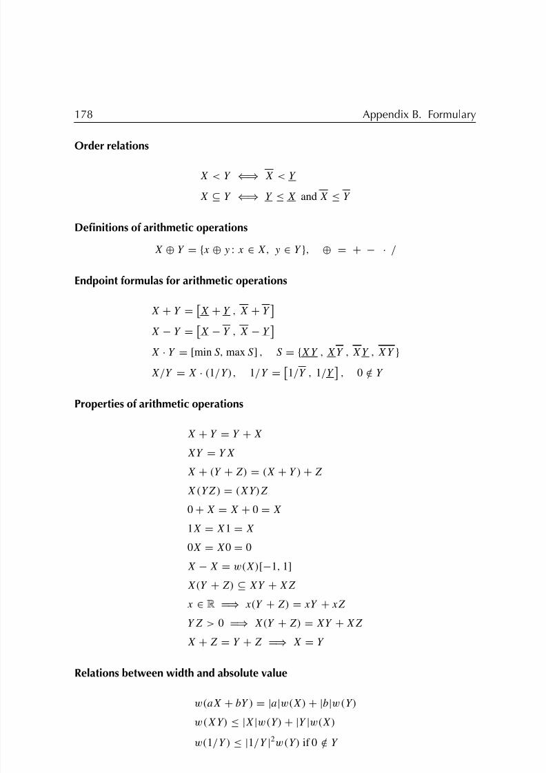
8/6/2019 Moore 1966
http://slidepdf.com/reader/full/moore-1966 189/234
178 Appendix B. Formulary
Order relations
X < Y ⇐⇒ X < Y
X ⊆ Y ⇐⇒ Y ≤ X and X ≤ Y
Definitions of arithmetic operations
X ⊕ Y = {x ⊕ y : x ∈ X, y ∈ Y }, ⊕ = + − · /
Endpoint formulas for arithmetic operations
X + Y =
X + Y , X + Y
X − Y =
X − Y , X − Y
X · Y = [min S, max S ] , S = {XY , XY , XY , XY }
X/Y = X · (1/Y), 1/Y =
1/Y , 1/Y
, 0 /∈ Y
Properties of arithmetic operations
X + Y = Y + X
XY = Y X
X + (Y + Z) = (X + Y ) + Z
X(YZ) = (XY)Z
0 + X = X + 0 = X
1X = X1 = X
0X = X0 = 0
X − X = w(X)[−1, 1]
X(Y + Z) ⊆ XY + XZ
x ∈ R =⇒ x(Y + Z) = xY + xZ
Y Z > 0 =⇒ X(Y + Z) = XY + XZ
X + Z = Y + Z =⇒ X = Y
Relations between width and absolute value
w(aX + bY ) = |a|w(X) + |b|w(Y)
w(XY) ≤ |X|w(Y) + |Y |w(X)
w(1/Y ) ≤ |1/Y |2w(Y) if 0 /∈ Y
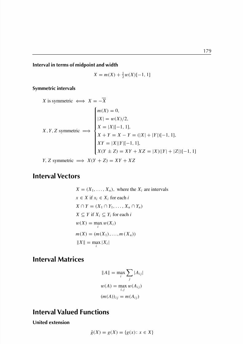
8/6/2019 Moore 1966
http://slidepdf.com/reader/full/moore-1966 190/234
179
Interval in terms of midpoint and width
X = m(X) + 12w(X)[−1, 1]
Symmetric intervals
X is symmetric ⇐⇒ X = −X
X,Y,Z symmetric =⇒
m(X) = 0,
|X| = w(X)/2,X = |X|[−1, 1],
X + Y = X − Y = (|X| + |Y |)[−1, 1],
XY = |X||Y |[−1, 1],
X(Y ± Z) = XY + XZ = |X|(|Y | + |Z|)[−1, 1]
Y, Z symmetric =⇒ X(Y + Z) = XY + XZ
Interval Vectors
X = (X1, . . . , Xn), where the Xi are intervals
x ∈ X if xi ∈ Xi for each i
X ∩ Y = (X1 ∩ Y 1, . . . , Xn ∩ Y n)
X ⊆ Y if Xi ⊆ Y i for each i
w(X) = maxi
w(Xi)
m(X) = (m(X1), . . . ,m(Xn))
X = maxi
|Xi |
Interval Matrices
A = maxi
j
|Aij |
w(A) = maxi,j
w(Aij)
(m(A))ij = m(Aij)
Interval Valued Functions
United extension
g(X) = g(X) = {g(x) : x ∈ X}

8/6/2019 Moore 1966
http://slidepdf.com/reader/full/moore-1966 191/234
180 Appendix B. Formulary
(The united extension is simply the exact range of g over X.)
Monotonicity
f(X) =
f(X),f(X)
, f increasing,
f(X),f(X)
, f decreasing
Inclusion isotonicity
Y i ⊆ Xi for each i =⇒ F (Y 1, . . . , Y n) ⊆ F (X1, . . . , Xn)
Fundamental theorem of interval analysis
F an inclusion isotonic
interval extension of f
=⇒ f (X1, . . . , Xn) ⊆ F (X1, . . . , Xn)
Power function
Xn = {xn : x ∈ X} =Xn, X
n
, X > 0 or n odd (or both),Xn, Xn
, X < 0 and n even,
[0, |X|n] , 0 ∈ X and n even
Sequences
Metric
d(X,Y) = max{|X − Y |, |X − Y |}
d(X,Y) = 0 ⇐⇒ X = Y
d(X,Y) = d(Y,X)
d(X,Y) ≤ d(X, Z) + d(Z,Y)
d(X + Z, Y + Z) = d(X,Y)
X ⊆ Y =⇒ d(X,Y) ≤ w(Y)
d(X, 0) = |X|
Convergence
∀ε > 0, ∃N such that n > N =⇒ d(Xk , X) < ε
Lipschitz condition
∃L such that X ⊆ X0 =⇒ w(F(X)) ≤ Lw(X)

8/6/2019 Moore 1966
http://slidepdf.com/reader/full/moore-1966 192/234
181
Uniform subdivision of interval vector
Xi,j =
Xi + (j − 1)w(Xi )/N , Xi + j w(Xi )/N
Xi = ∪N j =1Xi,j
w(Xi,j ) = w(Xi )/N
X = ∪N ji =1(X1,j1
, . . . , Xn,jn)
w(X1,j1, . . . , Xn,jn
) = w(X)/N
Refinement
F (N )(X) =N
ji =1 F (X1,j1, . . . , Xn,jn
)
Excess width
w(E(X)) = w(F(X)) − w(f (X))
Nested sequence
Xk+1 ⊆ Xk (k = 0, 1, 2, . . . )
Finite convergence in K steps
∃K such that k ≥ K =⇒ Xk = XK
Iteration
Xk+1 = F (Xk ) ∩ Xk (k = 0, 1, 2, . . . ) .
One-dimensional Newton’s method
X(k+1)= X(k)
∩ N (X(k) ), N (X) = m(X) − f (m(X))/F (X)
Here, m(X) may be replaced by any y ∈ X, and there may be advantages to doing so in
particular instances and for particular k.
IntegrationEndpoint formula
[a,b]
F(t)d t =
[a,b]
F(t) dt ,
[a,b]
F(t)d t

8/6/2019 Moore 1966
http://slidepdf.com/reader/full/moore-1966 193/234
182 Appendix B. Formulary
Polynomials
a, b have same sign =⇒
[a,b]
(A0 + · · · + Aq t q ) dt = A0(b − a) + · · · + Aq (bq+1 − aq+1)/(q + 1);
a, b have opposite signs =⇒
[a,b]
(A0 + · · · + Aq t q ) dt = T 0 + T 1 + · · · + T q , where
T i =
Ai (bi+1 − ai+1)/(i + 1), i even,
(Ai bi+1 − Aai+1)/(i + 1) , (Ai bi+1 − Aai+1)/(i + 1)
, i odd.
Enclosure by Taylor expansion
x(t) ∈
N −1k=0
(x)k (t − t 0)k + RN ([t 0, t ])(t − t 0)N ,
where RN ([t 0, t ]) is an interval enclosure for xN ([t 0, t ])
(x)0 = x(t 0), (x)k =1
k!
d kx
dt k(t 0)
Recursions for automatic differentiation
(uv)k =
kj =0
(u)j (v)k−j
(u/v)k =
1
v
(u)k −
kj =1
(v)j (u/v)k−j
(ua )k =
1
u
k−1j =0
a −
j (a + 1)
k
(u)k−j (ua )j
(eu)k =
k−1j =0
1 −
j
k
(eu)j (u)k−j

8/6/2019 Moore 1966
http://slidepdf.com/reader/full/moore-1966 194/234
183
(ln u)k =
1
u
(u)k −
k−1j=1
1−
j
k
(u)j (ln u)k−j
(sin u)k =
1
k
k−1j=0
(j + 1)(cosu)k−1−j (u)j+1
(cosu)k = −
1
k
k−1j=0
(j + 1)(sin u)k−1−j (u)j+1.

8/6/2019 Moore 1966
http://slidepdf.com/reader/full/moore-1966 195/234
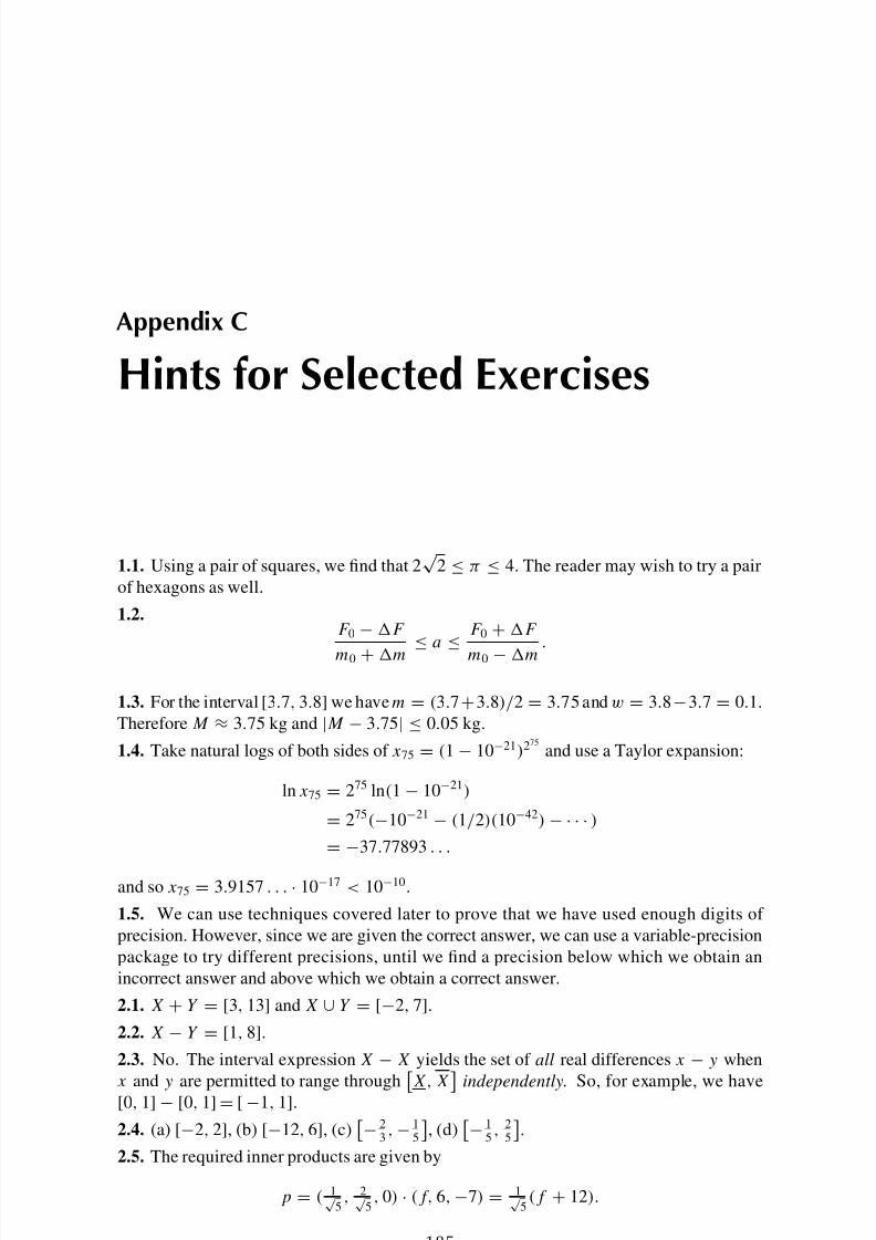
8/6/2019 Moore 1966
http://slidepdf.com/reader/full/moore-1966 196/234
Appendix C
Hints for Selected Exercises
1.1. Using a pair of squares, we find that 2√
2 ≤ π ≤ 4. The reader may wish to try a pair
of hexagons as well.
1.2.F 0 −F
m0 +m ≤a≤
F 0 +F
m0 −m.
1.3. For the interval [3.7, 3.8]we havem = (3.7+3.8)/2 = 3.75 andw = 3.8−3.7 = 0.1.
Therefore M ≈ 3.75 kg and |M − 3.75| ≤ 0.05 kg.
1.4. Take natural logs of both sides of x75 = (1 − 10−21)275
and use a Taylor expansion:
ln x75 = 275 ln(1 − 10−21)
= 275(−10−21 − (1/2)(10−42)− · · · )
= −37.77893 . . .
and so x75 = 3.9157 . . . · 10−17 < 10−10.
1.5. We can use techniques covered later to prove that we have used enough digits of
precision. However, since we are given the correct answer, we can use a variable-precision
package to try different precisions, until we find a precision below which we obtain an
incorrect answer and above which we obtain a correct answer.
2.1. X + Y = [3, 13] and X ∪ Y = [−2, 7].2.2. X − Y = [1, 8].2.3. No. The interval expression X − X yields the set of all real differences x − y when
x and y are permitted to range throughX, X
independently. So, for example, we have[0, 1] − [0, 1] = [ −1, 1].
2.4. (a) [−2, 2], (b) [−12, 6], (c)− 2
3,− 1
5
, (d)
− 1
5, 2
5
.
2.5. The required inner products are given by
p = ( 1√ 5, 2√
5, 0) · (f, 6,−7) = 1√
5(f + 12).
185
8/6/2019 Moore 1966
http://slidepdf.com/reader/full/moore-1966 197/234
8/6/2019 Moore 1966
http://slidepdf.com/reader/full/moore-1966 198/234
187
4.5. Take Z = [0, 2], X = [0, 1], and Y = [1, 1].
4.6.
X =
X, X
= 1
2(X + X) + 1
2(X − X)[−1, 1].
5.6. The command setround(-1) sets the rounding to “round down,” the command
setround(1) sets the rounding to “round up,” while the command setround(0) sets the
rounding to “round to the nearest machine number.” There is also some complication in
this routine, so it can handle arrays and complex interval arguments, and so it exits with
the machine in the same rounding mode as when the routine was entered. However, try to
identify the part where the lower and upper bounds of the interval value y are set.
5.8. If F is an interval extension of f such that F(x) = f(x) for real x, then F 1(X) =F(X) + X − X defines a different interval extension of f .
5.9. This can be done in various ways, plotting on a single window or in multiple windows.For example, plotting f in its own window could be done with the following sequence:
>> x = linspace(0.999,1.001);
>> y = x.ˆ6-6*x.ˆ5.+15.*x.ˆ4-20.*x.ˆ3.+15.*x.ˆ2-6.*x+1;
>> plot(x,y)
5.10. Setting p(x) = −5 + x2 = 0, we obtain x = ±√
5. Now√
5 is in [2, 3] and
furthermore, p(x)
=2x > 0 for x in
[2, 3
], so
√ 5 is a local minimum of p(x) for x in
[2, 3]. Since it is the only place in [2, 3] where p(x) = 0, it remains only to evaluate p(x)at the endpoints 2 and 3. Since p(2) = −6.3333 . . . and p(3) = −5, we obtain (5.28).
5.11. F ([0, 2]) =
12
, 32
, but F ([0, 1]) =
14
, 34
F ([0, 2]).
5.13. Since f (x) = x2 − 2, we have f (x) = 0 at x =√
2 ∈ [0, 3]. So f(x) has a
minimum value at x =√
2, namely, f (√
2) = − 43
√ 2. Now the maximum value is easily
seen to be f (3) = 3. Therefore f ([0, 3]) = [− 43
√ 2, 3]. With further calculation, we find
that f ([0, 3]) ⊆ [−1.88562, 3].
Without using calculus, we can find intervals enclosing the range of values found
above. First, f ([0, 3
])
⊆1
3 [0, 3
]3
−2[0, 3
] = [−6, 9
]. The form f(x)
=x( 1
3
x2
−2),
equivalent in real arithmetic, gives f ([0, 3]) ⊆ [0, 3]( 13[0, 3]2 − 2) = [0, 3][−2, 1] =
[−6, 3].
6.2. (a) We say that F(X) is continuous at X0 if for every ε > 0 there is a positive number
δ = δ(ε) such that d(F(X),F(X0)) < ε whenever d(X,X0) < δ. Here, again, d is the
interval metric given by (6.3).

8/6/2019 Moore 1966
http://slidepdf.com/reader/full/moore-1966 199/234

8/6/2019 Moore 1966
http://slidepdf.com/reader/full/moore-1966 200/234
189
Using this interval multiplier, the Gaussian formulas, evaluated in IA at the third or fourth
nonzero digit, yield the results
([1800, 2200] − (−[0.45, 0.55])(−[900, 1100]))I 2 = −5− (−[0.45, 0.55])10,
[1800, 2200]I 1 = 10 − (−[900, 1100])I 2,
so
[1195, 1795]I 2 = −5 + [4.5, 5.5] = [−0.5, 0.5]
and
I 2 = [1/1795, 1/1195][−0.5, 0.5] = [−0.000419, 0.000419]
and
I 1 = [1/2200, 1/1800](10 + [900, 1100][−0.000419, 0.000419])
= [1/2200, 1/1800](10 + [−0.4609, 0.4609])
= [1/2200, 1/1800][9.5291, 10.4609].
Our result is that the interval vector (I 1, I 2) encloses the set of all real vector solution points
for any real number choices of coefficients from the given interval coefficients, where
I 1 = [0.00433, 0.00582] and I 2 = [−0.000419, 0.000419].
8.3.
m(X(0))−[m(X(0))]2 − 2
2X(0)= 5 −
25 − 2
2[4, 6]= [ 17
8, 37
12].
8.6. (−∞,− 124] ∪ [ 1
3,∞).
8.7. We seek x such that x3 = 5x + 1. To find a good starting interval, examine the graphs
of y = x3
and y = 5x + 1.8.8. First note that an object with specific gravity < 1 will float. The given polynomial has
three real roots in the interval [−1, 3]. However, only a root lying in [0, 2] makes sense as
an answer. We find h = 1.22 ± 0.01.
8.10. In Case 1, although the numerator and denominator of the quotient 1/X are both real
numbers, we convert them to intervals to obtain a mathematically rigorous lower bound. (It
is necessary that the computed result contain the exact mathematical result.) Thus, 1/X is
computed with interval arithmetic, and the lower boundof that result is used to form the lower
bound of the semi-infinite interval. A similar technique is used for Case 2 and Case 3. Also,
the Cset model used in this function has underlying set of numbers the finite reals (i.e., it does
not include−∞and∞ as numbers). If the extended reals were used as the underlying model,then in Case 1 we would have Y2 = infsup(-Inf,-Inf), in Case 3 we would have Y2
= infsup(Inf,Inf), and in Case 4 we would have Y1 = infsup(-Inf,-Inf) and
Y2 = infsup(Inf,Inf). Caution should thus be exercised when using xreciprocal
in either case, since INTLAB follows the finite version of Cset theory in some cases, if one
interprets [NaN,NaN] as the empty set, but INTLAB does not follow it consistently: Try

8/6/2019 Moore 1966
http://slidepdf.com/reader/full/moore-1966 201/234
190 Appendix C. Hints for Selected Exercises
computing infsup(0,0)/infsup(-1,1), infsup(0,0)/infsup(0,0), etc. Also see
Note 3 on p. 114.
8.11. In the given equation f ( I ) = 0, the function f ( I ) can be simplified:
ln(109I ) = ln(109) + ln(I),
so
f ( I ) = 0.8922390 − I − 0.0052 ln(I).
f ( I ) is clearly negative for I > 1 and positive for I < 0.892239. Thus, there is exactly
one real positive zero in [0.8922390, 1.0]. We have
f (I ) = −1 − 0.0052/I
so starting with X = [0.892239, 1.0], we can compute an interval Newton iteration as
follows:
m(X) = 0.9461195,
f (m(X)) = 0.892239 − 0.9461195 − 0.0052 ln(0.9461195)
= −0.053592491,
f (X) = f ([0.892239, 1.0])
= −1 − 0.0052/[0.892239, 1.0]
= [−1.005828036, −1.0052],
N(X) = 0.9461195 − {−0.053592491/[−1.005828036, −1.0052]}
= [0.8928042, 0.8928376].
Intersecting that with X = [0.892239, 1.0] does not change it, because N(X) is already
contained in X. In fact it contains the unique solution to the problem and is already an
interval of width about 3 × 10⁻⁵.
8.12. Aberth’s RANGE yields the following solutions: (1) forthe search interval [1.25, 1.35],
the solution θi = 1.30958 radians (75.0334◦); (2) for the search interval [0.73, 0.9], the so-
lution θi = 0.76551 radians (43.8605◦).
8.13. As can be seen graphically, there are two solutions
X = ±
0.7071 · · ·
0.7071 · · ·
.
8.14. I = 0.94641, V = 1.071715.
8.15. There are three critical points: to five places they are (0.06264, 0.75824), (0.28537,
0.60975), and (0.88443, 0.21038).
To see that the starting box X0 = ([0, 1], [0, 1]) is large enough, superpose two plots
of x2 vs. x1: one from the first equation (involving the fifth-degree polynomial) and one fromthe second equation (straight line). It should be obvious that there are three intersection
points, all having x1 ∈ [0, 1]. Then return to the straight line equation to see that these
intersections all have x2 ∈ [0, 1] as well.
8.20. First, your results may differ, depending upon how INTLAB is set to display intervals.Observe the following dialogue:

8/6/2019 Moore 1966
http://slidepdf.com/reader/full/moore-1966 202/234
191
>> intvalinit(’DisplayMidrad’)
>> sqrt(infsup(-1,1))
intval ans = < 0.0000 + 0.0000i , 1.0000 >
>> intvalinit(’Display__’)
>> sqrt(infsup(-1,1))
intval ans = 0_.____ + 0_.____i
>> intvalinit(’DisplayInfsup’)
>> sqrt(infsup(-1,1))
intval ans = [ -1.0000 - 1.0000i , 1.0000 + 1.0000i ]
In the first case, the result is represented as a disk of radius 1 in the complex plane, while,in the last case, the result is represented as a rectangle in the complex plane, whose lower
left corner is −1 − i and whose upper right corner is 1 + i. Thus, INTLAB interprets sqrt
as being complex-valued for negative values of its argument. In fact, INTLAB uses the
principal value of the square root; you can see this when sqrt(infsup(-1,-1)) returns a
small region about i. This interpretation of the square root is appropriate in some contexts,
but not in others, such as in constraint propagation with real variables or in interval Newton
methods dealing with real variables.
9.1. For k odd we have
At k =
At k , At k
=t k A , t kA , t > 0,
t k A , t kA
, t < 0.
Therefore [a,b]
At k dt =
[a,0]
At k dt +
[0,b]
At k dt
=
[a,0]
At k dt ,
[a,0]
At k dt
+
[0,b]
At k dt ,
[0,b]
At k dt
=
[a,0]At k dt ,
[a,0]
At k dt
+
[0,b]At k dt ,
[0,b]
At k dt
=
−
ak+1
k + 1A , −
ak+1
k + 1A
+
bk+1
k + 1A ,
bk+1
k + 1A
=
bk+1A − ak+1A
k + 1,
bk+1A − ak+1A
k + 1
.
Note: The result is equivalent to
{bk+1/(k + 1)}A − {ak+1/(k + 1)}A, (*)
but this is not the same as {bk+1/(k + 1) − ak+1/(k + 1)}A. For example, if k = 3
and A = [1, 2], and [a, b] = [ −1, 1], then (*) is (1/4)[1, 2] − (1/4)[1, 2], which is
[−1/4, 1/4]—not [0, 0].
9.3. To 10 places, Aberth’s RANGE finds (a) 6.74300141925; (b) 0.6314179219.

8/6/2019 Moore 1966
http://slidepdf.com/reader/full/moore-1966 203/234

8/6/2019 Moore 1966
http://slidepdf.com/reader/full/moore-1966 204/234
193
9.11.
1
0
1−x1
0
1−x1−x2
0
(x21 + x2
2 + x23 )e−x1x2x3 dx3 dx2 dx1 = 0.04955715430˜.
10.3. (a) We can take Y (0) = [1, b] for b > 1 and find that
P (Y (0))(t) = 1 +
t
0
[1, b2] ds = 1 + [1, b2]t ⊆ [1, b] for t ∈ [0, (b − 1)/b2].
The maximum value that (b− 1)/b2 can have for any b ≥ 1 is 1/4 when b = 2. The exact
solution is y(t) = 1/(1− t), which blows up as t → 1. (b) The exact solution is y(t) = e−t .

8/6/2019 Moore 1966
http://slidepdf.com/reader/full/moore-1966 205/234

8/6/2019 Moore 1966
http://slidepdf.com/reader/full/moore-1966 206/234
Appendix D
Internet Resources
Interval analysis is a rapidly evolving area with an ever-expanding set of applications. Since
the subject is inherently computational, it is not surprising that the Internet has played an
essential role in its growth. The World Wide Web is replete with information on interval
analysis—both theoretical and applied—and the reader is strongly urged to explore as much
of this material as may interest him or her. The purpose of this appendix is merely to suggesttwo starting points.
Interval Computations Site
The Interval Computations site
http://www.cs.utep.edu/interval-comp/
serves as a main hub for the interval analysis community and is strongly recommended. It
enumerates various programming languages for interval analysis, provides links to interval
and related software packages, and lists homepages of some active interval researchers.
Interval Computations originated in 1995 during an international workshop held at El Paso,
Texas. According to Vladik Kreinovich, comaintainer of the site, its goal is to disseminate
information and facilitate collaboration between researchers both inside and outside the
interval community. There are two mirror sites: one at the University of Texas at El Paso
and one in Spain.
Web Page for This Book
The authors will maintain a web page at
http://www.siam.org/books/ot110
Here they will endeavor to offer current links to the computational tools mentioned in the
book (such as INTLAB, RANGE, and GlobSol), as well as other resources of interest to
the reader.
195

8/6/2019 Moore 1966
http://slidepdf.com/reader/full/moore-1966 207/234

8/6/2019 Moore 1966
http://slidepdf.com/reader/full/moore-1966 208/234
Appendix E
INTLAB Commands andFunctions
Here, we list some INTLAB commands and functions. Many MATLAB functions and
commands are overloaded in INTLAB, and not all of these may be listed here. MATLAB’s
help feature may provide information about whether a particular function can be applied to
intervals. For example, if you are interested in an interval extension of the sine function, you
can type help sin from a MATLAB command window. You will then see basic MATLABhelp for sin, along with a listing, in blue, of links to directories of definitions for other data
types. In particular, you will see help intval/sin.m. This indicates that there is support
for an interval version of sin. Click on this blue link for further information.
With INTLAB installed, it is useful to go through the INTLAB part of MATLAB’s
Help→Demos menu. Finally, information and various examples are available at the
INTLAB web page.
We have not included functions from INTLAB’s accurate sum, gradient, Hessian,
slope, and variable precision arithmetic toolboxes in this appendix. The information here
applies to version 5.5 of INTLAB (and, presumably, later versions).
Some Basic Commands
Here we let X denote an interval, and a, b, c, and d real numbers.
intvalinit(’DisplayInfsup’): inf-sup default display
intvalinit(’DisplayMidrad’): midpoint-radius default display
intvalinit(’Display_’): uncertainty representation default display
X = infsup(a,b): defines X as [a, b]
X = midrad(a,b): defines X as [c, d ] = [a − b, a + b]
+, -, *, /, \, ∧, : interval arithmetic operations, as defined in MATLAB. As in
MATLAB, these can be applied to matrices.
= = , > = , < = , > , < , ∼= : logical operators, as in MATLAB, but with interval inter-
pretations
197

8/6/2019 Moore 1966
http://slidepdf.com/reader/full/moore-1966 209/234
198 Appendix E. INTLAB Commands and Functions
Some Special Interval Functions
These are functions special to the interval computations. Many can be applied when X and
Y are interval vectors or matrices.
diam(X): width of X
hull(X,Y): interval hull of X and Y
in(X,Y): returns 1 if and only if X is in Y (X may be real or interval, and X and Y may
be matrices)
in0(X,Y): returns 1 if and only if X is in the interior of Y (X may be real or interval, and
X and Y may be matrices)
inf(X): lower bound on X
intersect(X,Y): intersection of X and Y
inv(A): interval inverse of the matrix A, if it can be computed
isempty(X): returns 1 if and only if X is the empty interval
isintval(X): returns 1 if and only if X is an interval data type
mag(X): magnitude of X (applied componentwise for arrays)
mid(A): midpoint of A
mig(X): mignitude of X
rad(X): radius of the interval X (half of diam(X))
sup(X):
upper bound onX
Some Standard Functions Implemented in INTLAB
These functions return interval bounds on the ranges of the corresponding real-valued func-
tions. The bounds are generally good approximations to the narrowest possible bounds.
abs asin coth sin
acos asinh csc sinh
acosh atan exp sqrt
acot atanh log sum
acoth cos log10 tan
acsc cosh log2 tanh
asec cot sec

8/6/2019 Moore 1966
http://slidepdf.com/reader/full/moore-1966 210/234
199
INTLAB’s Plotting Facilities
INTLAB has overloaded MATLAB’s plot, semilogx, and semilogy routines and also
has special routines plotintval and plotlinsol.
plot(x,Y), plot(X,y), plot(X,Y): For the abscissa vector x real and the correspond-
ing ordinate vector Y interval, the INTLAB version plots the lower bounds on Y and
the upper bounds on Y as curves, shading in between. For both X and Y intervals,
plot(X,Y) plots shaded boxes for each (Xi, Y i) pair. If X is interval and y is real,
plot(X,y) plots a horizontal line for each (X, y) pair.
semilogx(X,Y), semilogy(X,Y), loglog(X,Y): Overall, these behave as plot for
one or both of abscissa X and ordinate Y interval. However, when x is real and Y
is interval, the area between the lower bound curve and upper bound curve is not
shaded, as it is for plot. As in the versions that come with MATLAB, semilogx,
semilogy, and loglog plot the x-axis, y-axis, and both axes on a logarithmic scale,
respectively.
plotintval(X): If X is an n-dimensional complex interval vector, plotintval plots
each component as a circle in the complex plane. If X is a two-dimensional array of
real intervals with dimensions (2,N) representing lower bounds and upper bounds of an N -dimensional interval vector, plotintval plots each interval vector [X1,i, X2,i]
asaboxinthexy-plane. Neither the circles nor the boxes are shaded, but their outlines
are plotted in colors that cycle.
plotlinsol(A,B): This routine plots the solution set to an interval linear systemAX = B
in two unknowns. (Such a solution set is illustrated in Figure 7.1 on p. 89.) The actual
solution set is shaded, and the entire solution set is enclosed in its interval hull (the
narrowest possible interval vector enclosing the solution set).
Some Other MATLAB Functions Overloaded in INTLAB
The following is a partial list of additional MATLAB functions that can be applied to interval
data types:
diag isnan norm spdiags
dim isreal real spones
disp2str issparse repmat spy
display iszero reshape trace
find length numel transposefull imag relerr tril
isfinite logical size triu
isinf nonzeros sparse
Particularly noteworthy is INTLAB’s support for sparse matrices.

8/6/2019 Moore 1966
http://slidepdf.com/reader/full/moore-1966 211/234
200 Appendix E. INTLAB Commands and Functions
INTLAB’s Matrix-Vector Arithmetic
INTLAB uses midpoint-radius representation of intervals in matrix-vector multiplicationin such a way that the rounding mode (round down or round up) need not be switchedafter each individual interval-interval multiplication. However, a consequence is that theresult of the individual multiplications is not sharp. The results are sharp when the intervalsare symmetric about 0, e.g., [−3, 3], and such intervals occur in the Krawczyk method inE = I − YA when Y is a good approximation to m(A)−1 (see (7.7) on p. 91) or in (X− y)when y−m(X) (see (8.13) on p. 116). In other cases, the results can be far from exact. Forexample, to check Example 7.2 on p. 86, we see the following:
>> intvalinit(’FastIVmult’)
===> Fast interval matrix multiplication in use (maximum
overestimation factor 1.5 in radius)
>> A = [infsup(1,2) infsup(3,4)]
intval A =
[ 1.0000 , 2.0000 ] [ 3.0000 , 4.0000 ]
>> B = [infsup(5,6) infsup(7,8); infsup(9,10), infsup(11,12)]
intval B =
[ 5.0000 , 6.0000 ] [ 7.0000 , 8.0000 ]
[ 9.0000 , 10.0000 ] [ 11.0000 , 12.0000 ]
>> A*B
intval ans =
[ 31.0000 , 52.0000 ] [ 39.0000 , 64.0000 ]
intvalinit(’SharpIVmult’)
===> Slow but sharp interval matrix multiplication in use
>> A*B
intval ans =
[ 32.0000 , 52.0000 ] [ 40.0000 , 64.0000 ]
The startintlab.m file distributed with INTLAB may specify fast matrix-vector multi-
plication, so you will need to issue intvalinit(’SharpIVmult’) to get results that are
almost exact. Nonetheless, in contexts such as the Krawczyk method and for very large sys-
tems that are point matrices or almost point matrices, the fast multiplication is appropriate.INTLAB uses the fast multiplication internally for various computations.
Some Other INTLAB Routines
These implement some other useful features only in INTLAB, as well as certain less fun-
damental algorithms in interval computations:
circulant, gershgorin, lssresidual, toeplitz.
Users of INTLAB have contributed numerous other routines besides the ones listed here.For instance, Jiri Rohn has made publicly available an extensive library of routines for the
analysis of interval linear systems.

8/6/2019 Moore 1966
http://slidepdf.com/reader/full/moore-1966 212/234
References
[1] OliverAberth. Precise Numerical Methods Using C++. Academic Press, New York,1998.
[2] Oliver Aberth. Introduction to Precise Numerical Methods. Academic Press, NewYork, 2007.
[3] Azmy S. Ackleh, Edward J. Allen, Ralph Baker Kearfott, and Padmanabhan Se-shaiyer, editors. Classical and Modern Numerical Analysis: Theory, Methods, and
Practice. Taylor and Francis, Boca Raton, FL, 2009.
[4] Götz Alefeld. Intervallrechnung über den komplexen Zahlen und einige Anwendun-
gen. Dissertation, Universität Karlsruhe, Germany, 1968.
[5] Götz Alefeld. Bemerkungen zur Einschließung der Lösung eines linearen Gle-ichungssystems. Z. Angew. Math. Mech., 50:T33–T35, 1970.
[6] Götz Alefeld and Nikolaos Apostolatos. Praktische Anwendung von Ab-schätzunsformeln bei Iterationsverfahren. Z. Angew. Math. Mech., 48:T46–T49,1968.
[7] Götz Alefeld and Jürgen Herzberger. Über de Verbesserung von Schranken für dieLösung bei linearen Gleichungssystemen. Angew. Informatik (Elektron. Datenver-
arbeitung), 13:107–112, 1971.
[8] Götz Alefeld and Jürgen Herzberger. Zur Invertierung linearer und beschränkterOperatoren. Math. Zeitschr., 120:309–317, 1971.
[9] Götz Alefeld and Jürgen Herzberger. Einschließungsverfahren zur Berechnung desinversen Operators. Z. Angew. Math. Mech., 52:T197–T198, 1972.
[10] Götz Alefeld and Jürgen Herzberger. Nullstelleneinschließung mit dem Newton-Verfahren ohne Invertierung von Intervallmatrizen. Numer. Math., 19(1):56–64,Feb. 1972.
[11] Götz Alefeld and Jürgen Herzberger. Ein Verfahren zur monotonen Einschließungvon Lösungen nichtlinearer Gleichungssysteme. Z. Angew. Math. Mech., 53:T176–T177, 1973.
201

8/6/2019 Moore 1966
http://slidepdf.com/reader/full/moore-1966 213/234
202 References
[12] Götz Alefeld and Jürgen Herzberger. Einführung in die Intervallrechnung. Springer-Verlag, Berlin, 1974.
[13] Götz Alefeld and Jürgen Herzberger. Introduction to Interval Computations. Aca-demic Press, New York, 1983.
[14] Götz Alefeld, Jürgen Herzberger, and Otto Mayer. Über neuere Gesichtspunkte beimnumerischen Rechnen. Math. Naturw. Unterricht , 24:458–467, 1971.
[15] Nikolaos Apostolatos and Ulrich W. Kulisch. Approximation der erweiterten Inter-
vallarithmetik durch die einfache Maschinenintervallarithmetik.Computing
, 2:181–194, 1967.
[16] Nikolaos Apostolatos and Ulrich W. Kulisch. Grundlagen einer Maschineninterval-larithmetik. Computing, 2:89–104, 1967.
[17] Nikolaos Apostolatos and Ulrich W. Kulisch. Grundzüge einer Intervallrechnung fürMatrizen und einige Anwendungen. Elektronische Rechenanlagen, 10:73–83, 1968.
[18] NikolaosApostolatos, UlrichW. Kulisch, Rudolf Krawczyk, B. Lortz, Karl L. Nickel,and Hans-Wilm Wippermann. The algorithmic languageTriplex-ALGOL 60. Numer.
Math., 11(2):175–180, Feb. 1968.
[19] NikolaosApostolatos, Ulrich W. Kulisch, and KarlL. Nickel. Ein Einschliessungsver-fahren für Nullstellen. Computing, 2:195–201, 1967.
[20] Eckart Baumann. Optimal centered forms. BIT , 28(1):80–87, 1988.
[21] Martin Berz, Christian Bischof, George F. Corliss, and Andreas Griewank, edi-tors. Computational Differentiation: Techniques, Applications, and Tools. SIAM,Philadelphia, 1996.
[22] Martin Berz and Kyoko Makino. Higher order multivariate automatic differentiation
and validated computation of remainder bounds. WSEAS Trans. Math., 3(1):37–44,Jan. 1998.
[23] Martin Berz and Kyoko Makino. New methods for high-dimensional verified quadra-ture. Reliable Computing, 5:13–22, Feb. 1999.
[24] Martin Berz and Kyoko Makino. Performance of Taylor model methods for validatedintegration of ODEs. In Jack Dongarra, Kaj Madsen, and Jerzy Wasniewski, editors,Applied Parallel Computing, Lecture Notes in Computer Science 3732, Springer-Verlag, New York, 2005, pp. 65–74.
[25] Martin Berz, Kyoko Makino, and Youn-Kyung Kim. Long-term stability of the teva-tron by verified global optimization. Nuclear Instruments Methods Physics Research
A, 558:1–10, March 2006.
[26] W. Binstock, J. Hawkes, and N.-T. Hsu. An Interval Input / Output Package for the
Univac 1108. Technical Report 1212, Mathematics Research Center, University of Wisconsin, Sept. 1973.
8/6/2019 Moore 1966
http://slidepdf.com/reader/full/moore-1966 214/234
References 203
[27] Folkmar Bornemann, Dirk Laurie, Stanley Wagon, and Jörg Waldvogel. The SIAM
100-Digit Challenge: A Study in High-Accuracy Numerical Computing. SIAM,
Philadelphia, 2004.
[28] Glencora Borradaile and Pascal Van Hentenryck. Safe and tight linear estimators for
global optimization. Math. Program., 102(3):495–517, 2005.
[29] Norbert C. Börsken. Komplexe Kreis-Standardfunktionen. Dissertation, Universität
Freiburg, Freiburg, Germany, 1978.
[30] Judy A. Braun and Ramon E. Moore. A Program for the Solution of Differential
Equations Using Interval Arithmetic (DIFEQ) for the CDC 3600 and 1604. Technical
Report 901, Mathematics Research Center, University of Wisconsin, Dec. 1967.
[31] Robert P. Broadwater, Hesham E. Shaalan, and Wolter J. Fabrycky. Decision evalua-
tion with interval mathematics: A power distribution system case study. IEEE Trans.
Power Systems, 20(2):725–7334, May 2005.
[32] Ole Caprani, Kaj Madsen, and Louis B. Rall. Integration of Interval Functions. SIAM
J. Math. Anal., vol 2: 321–341, 1981.
[33] Ole Caprani, Kaj Madsen, and Louis B. Rall. Integration of interval functions. SIAM
J. Math. Anal., 12(3):321–341, 1981.
[34] Damien Chablat, Philippe Wenger, Félix Majou, and Jean-Pierre Merlet. An interval
analysis based study for the design and the comparison of three-degrees-of-freedom
parallel kinematic machines. I. J. Robotic Res., 23(6):615–624, 2004.
[35] Su Huan Chen, Hua Dong Lian, and Xiao Wei Yang. Interval eigenvalue analysis
for structures with interval parameters. Finite Elements Anal. Design, 39:419–431,
March 2003.
[36] Bruce Christianson. Reverse accumulation and accurate rounding error estimates for
Taylor series coefficients. Optimization Methods and Software, 1(1):81–94, 1991.
[37] Amanda E. Connell and Robert. M. Corless. An experimental interval arithmetic
package in Maple. Interval Comput., 2:120–134, 1993.
[38] George F. Corliss, Christèle Faure, Andreas Griewank, Laurent Hascoët, and Uwe
Naumann, editors. Automatic Differentiation of Algorithms: From Simulation to
Optimization. Computer and Information Science. Springer, New York, 2001.
[39] George F. Corliss, Christopher Foley, and Ralph Baker Kearfott. Formulation for
reliable analysis of structural frames. Reliable Comput., 13:125–147, April 2007.
[40] George F. Corliss and Louis B. Rall. Adaptive, self-validating numerical quadrature.
SIAM J. Sci. Statist. Comput., 8(5):831–847, 1987.
[41] I. Csajka, W. Muenzer, and Karl L. Nickel. Subroutines add, neg, sub, div, mul,
for Use in an Error-Bound Arithmetic. Technical report, IBM Research Laboratory,
Rueschlikon, Switzerland, 1966.

8/6/2019 Moore 1966
http://slidepdf.com/reader/full/moore-1966 215/234
204 References
[42] Brian Davies. Whither mathematics? Notices Amer. Math. Soc., 52(11):1350–1356,
Dec. 2005.
[43] Kaisheng Du. Cluster Problem in Global Optimization Using Interval Arithmetic.
Ph.D. thesis, University of Southwestern Louisiana, 1994.
[44] Kaisheng Du and Ralph Baker Kearfott. The cluster problem in global optimization:
The univariate case. Computing (Suppl.), 9:117–127, 1992.
[45] Bo Einarsson, editor. Accuracy and Reliability in Scientific Computing. SIAM,
Philadelphia, 2005.
[46] Andrea Fusiello, Arrigo Benedetti, Michela Farenzena, and Alessandro Busti. Glob-
ally convergent autocalibration using interval analysis. IEEE Trans. Pattern Anal.
Mach. Intell., 26(12):1633–1638, 2004.
[47] Irene Gargantini and Peter Henrici. Circular arithmetic and the determination of
polynomial zeros. Numer. Math., 18(4):305–320, Aug. 1972.
[48] Chao-Yang Gau and Mark A. Stadtherr. Dynamic load balancing for parallel interval-
Newton using message passing. Comput. Chemical Engrg., 26:811–815, June 2002.
[49] Chao-Yang Gau and Mark A. Stadtherr. New interval methodologies for reliablechemical process modeling. Comput. Chemical Engrg., 26:827–840, June 2002.
[50] Gene H. Golub and Charles F. van Loan. Matrix Computations, 3rd ed. Johns Hopkins
University Press, Baltimore, 1996.
[51] Laurent Granvilliers and Frédéric Benhamou. Progress in the solving of a circuit
design problem. J. Global Optim., 20:155–168, June 2001.
[52] Laurent Granvilliers and Frédéric Benhamou. Algorithm 852: RealPaver: An interval
solver using constraint satisfaction techniques. ACM Trans. Math. Softw., 32(1):138–
156, 2006.
[53] Andreas Griewank. Evaluating Derivatives: Principles and Techniques of Algorith-
mic Differentiation. Frontiers in Appl. Math., 19, SIAM, Philadelphia, 2000.
[54] Andreas Griewank and George F. F. Corliss, editors. Automatic Differentiation of
Algorithms: Theory, Implementation, and Application. SIAM, Philadelphia, 1991.
[55] Angelika C. Hailer. Verification of Branch and Bound Algorithms Applied to Water
Distribution Network Design. Logos Verlag, Berlin, 2006. Dissertation, Technische
Universität Hamburg, Harburg.
[56] Rolf Hammer, Matthias Hocks, Ulrich W. Kulisch, and Dietmar Ratz. Numerical
Toolbox for Verified Computing I—Basic Numerical Problems. Springer-Verlag,
Heidelberg, 1993.
[57] E. Hansen and G. W. Walster. Global Optimization Using Interval Analysis. Marcel
Dekker, New York, 2003.

8/6/2019 Moore 1966
http://slidepdf.com/reader/full/moore-1966 216/234
References 205
[58] Eldon R. Hansen. Interval arithmetic in matrix computations, part I. J. Soc. Indust.
Appl. Math. Ser. B Numer. Anal., 2(2):308–320, 1965.
[59] Eldon R. Hansen. On solving systems of equations using interval arithmetic. Math.
Comput., 22(102):374–384, April 1968.
[60] Eldon R. Hansen. The centered form. In Eldon R. Hansen, editor, Topics in Interval
Analysis, Oxford University Press, London, 1969, pp. 102–106.
[61] Eldon R. Hansen. On linear algebraic equations with interval coefficients. In Eldon R.
Hansen, editor, Topics in Interval Analysis, Oxford University Press, London, 1969,pp. 35–46.
[62] Eldon R. Hansen. On solving two-point boundary-value problems using interval
arithmetic. In Eldon R. Hansen, editor, Topics in Interval Analysis, Oxford University
Press, London, 1969, pp. 74–90.
[63] Eldon R. Hansen. Topics in Interval Analysis. Oxford University Press, London,
1969.
[64] Eldon R. Hansen. Interval forms of Newton’s method. Computing, 20:153–163,
1978.
[65] Eldon R. Hansen. Global Optimization Using Interval Analysis. Marcel Dekker,
New York, 1992.
[66] Eldon R. Hansen and Saumyendra Sengupta. Bounding solutions of systems of
equations using interval analysis. BIT (Nordisk tidskrift for informationsbehandling),
21(2):203–211, June 1981.
[67] Eldon R. Hansen and Roberta Smith. A Computer Program for Solving a System
of Linear Equations and Matrix Inversion with Automatic Error Bounding Using
Interval Arithmetic. Technical Report LMSC 4-22-66-3, Lockheed Missiles and
Space Co., Palo Alto, CA, 1966.
[68] Eldon R. Hansen and Roberta Smith. Interval arithmetic in matrix computations, part
II. SIAM J. Numer. Anal., 4(1):1–9, March 1967.
[69] Eldon R. Hansen and G. William Walster. Global optimization in nonlinear mixed
integer problems. In William F. Ames and R. Vichnevetsky, editors, Proceedings of
the 10th IMACS World Congress on Systems Simulation and Scientific Computing,
vol. 1, IMACS, Plantation, FL, 1982, pp. 379–381.
[70] G. I. Hargreaves. Interval Analysis in MATLAB. Master’s thesis, Department of
Mathematics, University of Manchester, 2002.
[71] Joel Hass, Michael Hutchings, and Roger Schlafly. The double bubble conjecture.
Electronic Research Announcements of the American Mathematical Society, 1:98–
102, 1995.

8/6/2019 Moore 1966
http://slidepdf.com/reader/full/moore-1966 217/234

8/6/2019 Moore 1966
http://slidepdf.com/reader/full/moore-1966 218/234
References 207
[88] William M. Kahan. Circumscribing an ellipsoid about the intersection of two ellip-
soids. Can. Math. Bull., 11:437–441, 1968.
[89] William M. Kahan. A More Complete Interval Arithmetic: Lecture Notes for an
Engineering Summer Course in Numerical Analysis at the University of Michigan.
Technical report, University of Michigan, 1968.
[90] William M. Kahan. Invited commentary (concerning the invited paper of Karl L.
Nickel: Error bounds and computer arithmetic). In A. Morrell, editor, Proceedings
of IFIP Congress 1968, vol. I, North–Holland, Amsterdam, 1969, pp. 60–62.
[91] William M. Kahan. A survey of error analysis. In C. V. Freiman, J. E. Griffith, and
J. L. Rosenfeld, editors, Proceedings of IFIP Congress 1971, vol. II, North–Holland,
Amsterdam, 1972, pp. 1214–1239.
[92] Leonid Vitalevich Kantorovich. On a mathematical symbolism convenient for per-
forming machine calculations (in Russian). Dokl. Akad. Nauk SSSR, 113(4):738–741,
1957.
[93] Ralph Baker Kearfott. Abstract generalized bisection and a cost bound. Math.
Comput., 49(179):187–202, July 1987.
[94] Ralph Baker Kearfott. Some tests of generalized bisection. ACM Trans. Math.
Software, 13(3):197–220, Sept. 1987.
[95] Ralph Baker Kearfott. Corrigenda: Some Tests of Generalized Bisection. ACM
Trans. Math. Software, 14(4):399–399, Dec. 1988.
[96] Ralph Baker Kearfott. Algorithm 763: INTERVAL_ARITHMETIC: A Fortran 90
module for an interval data type. ACM Trans. Math. Software, 22(4):385–392, Dec.
1996.
[97] Ralph Baker Kearfott. Rigorous Global Search: Continuous Problems. Nonconvex
Optimization and Its Applications 13, Kluwer Academic Publishers, Dordrecht, TheNetherlands, 1996.
[98] Ralph Baker Kearfott. On proving existence of feasible points in equality constrained
optimization problems. Math. Program., 83(1):89–100, 1998.
[99] Ralph Baker Kearfott. GlobSol User Guide, 2008. To appear in Optim. Methods
Software.
[100] Ralph Baker Kearfott. Verified branch and bound for singular linear and nonlinear
programs: An epsilon-inflation process, April 2007. Available from the author.
[101] Ralph Baker Kearfott, Milinde Dawande, Kaisheng Du, and Chenyi Hu. Algorithm
737: INTLIB: A portable Fortran-77 elementary function library. ACM Trans. Math.
Software, 20(4):447–459, Dec. 1994.
[102] Ralph Baker Kearfott and Kaisheng Du. The cluster problem in multivariate global
optimization. J. Global Optim., 5:253–265, 1994.
8/6/2019 Moore 1966
http://slidepdf.com/reader/full/moore-1966 219/234
208 References
[103] Ralph Baker Kearfott and Vladik Kreinovich, editors. Applications of Interval Com-
putations: Papers Presented at an International Workshop in El Paso, Texas, February
23–25, 1995, Applied Optimization 3, Kluwer, Dordrecht, The Netherlands, 1996.
[104] Ralph Baker Kearfott, Markus Neher, Shin’ichi Oishi, and Fabien Rico. Libraries,
tools, and interactive systems for verified computations: Four case studies. Lecture
Notes in Comput. Sci., 2991, Springer-Verlag, New York, 2004, pp. 36–63.
[105] Ralph Baker Kearfott and Manuel Novoa III. Algorithm 681: INTBIS, a portable
interval Newton/bisection package. ACM Trans. Math. Software, 16(2):152–157,
June 1990.
[106] Ralph Baker Kearfott and G. William Walster. On stopping criteria in verified nonlin-
ear systems or optimization algorithms. ACM Trans. Math. Software, 26(3):373–389,
Sept. 2000.
[107] Gershon Kedem. A posteriori error bounds for two-point boundary value problems.
SIAM J. Numer. Anal., 18(3):431–448, June 1981.
[108] Christian Keil and Christian Jansson. Computational experience with rigorous error
bounds for the netlib linear programming library. Reliable Comput., 12(4):303–321,
2006.
[109] J. B. Keiper. Interval arithmetic in Mathematica. Interval Comput., 1993(3):76–87,
1993.
[110] Hassan K. Khalil. Nonlinear Systems. MacMillan, New York, 1992.
[111] Olaf Knüppel. PROFIL/BIAS—A fast interval library. Computing, 53(3–4):277–287,
Sept. 1994.
[112] Olaf Knüppel. PROFIL/BIAS v 2.0. Bericht 99.1, Technische Universität Hamburg-
Harburg, Harburg, Germany, Feb. 1999.
[113] Martin Koeber. Inclusion of solutions of Darboux problems for quasilinear hyperbolic
equations. J. Comput. Appl. Math., 152:243–262, March 2003.
[114] Lubo Kolev. Interval Methods for Circuit Analysis. World Scientific, Singapore,
2003.
[115] Hasan Ugur Köylüoglu, Ahmet S. Çakmak, and Søren R. K. Neilson. Interval algebra
to deal with pattern loading and structural uncertainty. J. Engrg. Mech., 121:1149–
1157, 1995.
[116] Walter Krämer. intpakX—An Interval Arithmetic Package for Maple. In Proceedings
of the 12th GAMM, IMACS International Symposium on Scientific Computing, Com-
puter Arithmetic and Validated Numerics (SCAN 2006), IEEE Computer Society,
Washington, DC, 2006, p. 26.
[117] Walter Krämer, UlrichW. Kulisch, and Rudolf Lohner. Numerical Toolbox for Verified
Computing II: Advanced Numerical Problems. Springer-Verlag, New York, 2006.

8/6/2019 Moore 1966
http://slidepdf.com/reader/full/moore-1966 220/234
References 209
[118] Walter Krämer and Stefan Wedner. Two adaptive Gauss–Legendre type algorithms
for the verified computation of definite integrals. Reliable Comput., 2(3):241–254,
1996.
[119] Rudolf Krawczyk. Newton-Algorithmen zur Bestimmung von Nullstellen mit Fehler-
schranken. Interner Bericht des Inst. für Informatik 68/6, Universität Karlsruhe, 1968.
Computing, 4:187–201, 1969.
[120] Rudolf Krawczyk and Arnold Neumaier. Interval slopes for rational functions and
associated centered forms. SIAM J. Numer. Anal., 22(3):604–616, June 1985.
[121] Vladik Kreinovich, Anatoly Lakeyev, Jiri Rohn, and Patrick Kahl. Computational
Complexity and Feasibility of Data Processing and Interval Computations, Applied Optimization 10, Kluwer Academic Publishers, Dordrecht, The Netherlands, 1998.
[122] Ulrich W. Kulisch. An axiomatic approach to rounded computations. Numer. Math.,18:1–17, 1971.
[123] Ulrich W. Kulisch. Grundzüge der Intervallrechnung. In Detlef Laugwitz, editor,
Überblicke Mathematik 2, Bibliographisches Institut, Mannheim, 1969, pp. 51–98.
[124] Ulrich W. Kulisch. Interval Arithmetic Over Completely Ordered Ringoids. TechnicalReport 1105, Mathematics Research Center, University of Wisconsin, May 1972.
[125] Ulrich W. Kulisch and Willard L. Miranker. Computer Arithmetic in Theory and Practice. Academic Press, New York, 1981.
[126] Ulrich W. Kulisch and Willard L. Miranker. The arithmetic of the digital computer:
A new approach. SIAM Rev., 28(1):1–40, March 1986.
[127] Thomas D. Ladner and J. Michael Yohe. An Interval Arithmetic Package for theUnivac 1108. Technical Report 1055, Mathematics Research Center, University of
Wisconsin, Aug. 1970.
[128] Bruno Lang. Verified quadrature in determining Newton’s constant of gravitation.
J. Universal Comput. Sci., 4(1):16–24, Jan. 1998.
[129] Bruno Lang. Derivative-based subdivision in multi-dimensional verified Gaussian
quadrature. In Götz Alefeld, Jiri Rohn, Siegfried M. Rump, and Tetsuro Yamamoto,
editors, Symbolic Algebraic Methods and Verification Methods, Springer-Verlag,
New York, 2001, pp. 145–152.
[130] Yahia Lebbah, Claude Michel, Michel Rueher, David Daney, and Jean-Pierre Merlet.
Efficient and safe global constraints for handling numerical constraint systems. SIAM J. Numer. Anal., 42(5):2076–2097, 2005.
[131] Eric Lee, Constantinos Mavroidis, and Jean-Pierre Merlet. Five precision point
synthesis of spatial RRR manipulators using interval analysis. J. Mech. Design,
126:842–849, 2004.

8/6/2019 Moore 1966
http://slidepdf.com/reader/full/moore-1966 221/234
210 References
[132] Michael Lerch, German Tischler, Jürgen Wolff von Gudenberg, Werner Hofschus-
ter, and Walter Krämer. FILIB++, a fast interval library supporting containment
computations. ACM Trans. Math. Software, 32(2):299–324, June 2006.
[133] Youdong Lin, JoshuaA. Enszer, and Mark A. Stadtherr. Enclosing all solutions of two-
point boundary value problems for ODEs. Comput. Chemical Engrg., 32(8):1714–
1725, August 2008.
[134] Youdong Lin and Mark A. Stadtherr. Advances in interval methods for deterministic
global optimization in chemical engineering. J. Global Optim., 29:281–296, July
2004.
[135] Youdong Lin and Mark A. Stadtherr. Locating stationary points of sorbate-zeolite
potential energy surfaces using interval analysis. J. Chem. Phys., 121:10159–10166,
2004.
[136] Youdong Lin and Mark A. Stadtherr. LP strategy for interval-Newton method in
deterministic global optimization. Ind. Engrg. Chem. Res., 43:3741–3749, 2004.
[137] Youdong Lin and Mark A. Stadtherr. Deterministic global optimization of molecular
structures using interval analysis. J. Comput. Chem., 26:1413–1420, 2005.
[138] Kyoko Makino and Martin Berz. Taylor models and other validated functional in-
clusion methods. Internat. J. Pure Appl. Math., 4,4:379–456, 2003.
[139] Kyoko Makino and Martin Berz. Suppression of the wrapping effect by Taylor model-
based verified integrators: Long-term stabilization by preconditioning. Int. J. Differ.
Equ. Appl., 10(4):353–384, 2005.
[140] Günter Mayer. Direct methods for linear systems with inexact input data, 2008. To
appear in Japan J. Industrial Appl. Math.
[141] Keith Meintjes and Alexander P. Morgan. A Methodology for Solving Chemical
Equilibrium Systems. General Motors Research Report GMR-4971. General MotorsResearch Laboratories, Warren, MI, 1985.
[142] Jean-Pierre Merlet. ALIAS: An interval analysis based library for solving and ana-
lyzing system of equations. In SEA, Toulouse, June 2000.
[143] Kenneth R. Meyer and Dieter S. Schmidt, editors. ComputerAided Proofs in Analysis.
Springer-Verlag, New York, 1991.
[144] Mehdi Modares, Robert L. Mullen, Paul X. Bellini, and R. Muhanna. Buckling anal-
ysis of structures with interval uncertainties. SAE Transactions Journal of Passenger
Cars—Mechanical Systems, March 1996, pp. 284–290.
[145] Cleve B. Moler. Numerical Computing with MATLAB. SIAM, Philadelphia, 2004.
[146] Ramon E. Moore. Interval Arithmetic and Automatic Error Analysis in Digital Com-
puting. Ph.D. dissertation, Department of Mathematics, Stanford University, Stan-
ford, CA, 1962.

8/6/2019 Moore 1966
http://slidepdf.com/reader/full/moore-1966 222/234
8/6/2019 Moore 1966
http://slidepdf.com/reader/full/moore-1966 223/234
8/6/2019 Moore 1966
http://slidepdf.com/reader/full/moore-1966 224/234
8/6/2019 Moore 1966
http://slidepdf.com/reader/full/moore-1966 225/234
214 References
[193] Michael Plum. Computer-assisted enclosure methods for elliptic differential
equations. Linear Algebra and Its Applications, 324:147–187, Feb. 2001.
[194] John Derwent Pryce and George F. Corliss. Interval arithmetic with containment
sets. Computing, 78(3):251–276, 2006.
[195] Louis B. Rall, editor. Error in Digital Computation, vol. I. Wiley, New York, 1965.
[196] Louis B. Rall, editor. Error in Digital Computation, vol. II. Wiley, New York, 1965.
[197] Louis B. Rall. Application of interval integration to the solution of integral equations. J. Integral Equations, 6:127–141, 1984.
[198] Louis B. Rall. Representations of intervals and optimal error bounds. Math. Comput.,
41:219–227, 1983.
[199] Louis B. Rall. Application of interval integration to the solution of integral equations
II—the finite case. SIAM J. Math. Anal., 13:690–697, 1982.
[200] Louis B. Rall. Automatic Differentiation: Techniques and Applications. Lecture
Notes in Computer Science 120. Springer-Verlag, Berlin, 1981.
[201] Louis B. Rall. Interval analysis: A new tool for applied mathematics. In Transactions
of the Twenty-Seventh Conference of Army Mathematicians, Army Research Office,
Research Triangle Park, NC, 1982, pp. 283–301.
[202] Louis B. Rall. Mean value and Taylor forms in interval analysis. SIAM J. Math.
Anal., 14:223–238, 1983.
[203] Louis B. Rall. Solution of Finite Systems of Equations by Interval Iteration. Technical
Report 2271, Mathematics Research Center, University of Wisconsin, Aug. 1981.
[204] Louis B. Rall. A theory of interval iteration. Proceedings of the American Mathematical Society, 86:625–631, 1982.
[205] Louis B. Rall. Interval bounds for stationary values of functionals. Nonlinear Anal.,
6:855–861, 1982.
[206] Louis B. Rall. Interval methods for fixed-point problems. Numerical Functional
Analysis and Optimization, 9:35–59, 1987.
[207] Louis B. Rall. Global Optimization Using Automatic Differentiation and Interval
Iteration. Technical Report 2832, Mathematics Research Center, University of
Wisconsin, June 1985.
[208] Louis B. Rall. Improved interval bounds for ranges of functions. Lecture Notes
in Comput. Sci. 212, Karl L. Nickel, editor, Springer-Verlag, New York, 1986,
pp. 143–155.
[209] Helmut Ratschek. Centered forms. SIAM J. Numer. Anal., 17(5):656–662, 1980.

8/6/2019 Moore 1966
http://slidepdf.com/reader/full/moore-1966 226/234
References 215
[210] Helmut Ratschek and Jon G. Rokne. Computer Methods for the Range of Functions.
Ellis Horwood Ser.: Math. Appl. Ellis Horwood, Chichester, UK, 1984.
[211] Helmut Ratschek and Jon G. Rokne. New Computer Methods for Global
Optimization. Wiley, New York, 1988.
[212] Helmut Ratschek and Jon G. Rokne. Experiments using interval analysis for solving
a circuit design problem. J. Global Optim., 3:501–518, Dec. 1993.
[213] Dietmar Ratz. Automatic Slope Computation and Its Application in Nonsmooth
Global Optimization. Shaker Verlag, Aachen, 1998.
[214] Gerald Recktenwald. Numerical Methods with MATLAB: Implementations and
Applications. Prentice–Hall, Englewood Cliffs, NJ, 2000.
[215] Allen Reiter. Interval Arithmetic Package (INTERVAL) for the CDC 1604 and
CDC 3600. Technical Report 794, Mathematics Research Center, University of
Wisconsin, Dec. 1967.
[216] Thomas W. Reps and Louis B. Rall. Computational divided differencing and divided-
difference arithmetics. Higher Order Symbol. Comput., 16(1-2):93–149, 2003.
[217] Nathalie Revol and Fabrice Rouillier. Motivations for an arbitrary precision interval
arithmetic and the MPFI library. Reliable Comput., 11(4):275–290, 2005.
[218] Siegfried M. Rump. Kleine Fehlerschranken bei Matrixproblemen. Dissertation,
Universität Karlsruhe, Germany, 1980.
[219] Siegfried M. Rump. Solving algebraic systems with high accuracy. In Ulrich W.
Kulisch and Willard L. Miranker, editors, A New Approach to Scientific Computation,
Academic Press, New York, 1983, pp. 51–120.
[220] Siegfried M. Rump. Algebraic Computation, Numerical Computation and Verified
Inclusions. In R. Janssen, editor, Trends in Computer Algebra, Lecture Notes in
Computer Science 296, 1988, pp. 177–197.
[221] Siegfried M. Rump. Verification methods for dense and sparse systems of equations.
In Jürgen Herzberger, editor, Topics in Validated Computations: Proceedings of
IMACS-GAMM International Workshop on Validated Computation, Oldenburg,
Germany, 30 August–3 September 1993, Studies in Computational Mathematics 5,
Elsevier, Amsterdam, The Netherlands, 1994, pp. 63–136.
[222] Siegfried M. Rump. Expansion and estimation of the range of nonlinear functions.
Math. Comput., 65(216):1503–1512, Oct. 1996.
[223] Siegfried M. Rump. Fast and parallel interval arithmetic. BIT Numer. Math.,
39(3):534–554, Sep. 1999.
8/6/2019 Moore 1966
http://slidepdf.com/reader/full/moore-1966 227/234
216 References
[224] Siegfried M. Rump. INTLAB–INTerval LABoratory. In Tibor Csendes, editor,
Developments in Reliable Computing: Papers presented at the International Sym-
posium on Scientific Computing, Computer Arithmetic, and Validated Numerics,
SCAN-98, in Szeged, Hungary, Reliable Computing 5(3), Kluwer Academic
Publishers, Dordrecht, The Netherlands, 1999, pp. 77–104.
[225] Siegfried M. Rump. Rigorous and portable standard functions. BIT Numer. Math.,
41(3):540–562, June 2001.
[226] Siegfried M. Rump and Takeshi Ogita. Super-fast validated solution of linear
systems. J. Comput. Appl. Math., 199(2):199–206, 2007.
[227] Nikolaos V. Sahinidis. BARON: A general purpose global optimization software
package. J. Global Optim., 8(2):201–205, 1996.
[228] Hermann Schichl and Arnold Neumaier. Exclusion regions for systems of equations.
SIAM J. Numer. Anal., 42(1):383–408, 2004.
[229] Marco Schnurr. Steigungen höherer Ordnung zur verifizierten globalen Optimierung.
Ph.D. dissertation, Department of Mathematics, University of Karlsruhe, Germany,
May 2007.
[230] Hesham E. Shaalan and Robert P. Broadwater. Using interval mathematics in cost
benefit analysis of distribution automation. Electric Power Systems Research,
27:145–152, 1993.
[231] Zhixin Shi and Brian Hassard. Precise solution of Laplace’s equation. Math.
Comput., 64(210):515–536, April 1995.
[232] Stig Skelboe. Computation of rational interval functions. BIT , 14:187–195, 1974.
[233] John M. Snyder. Generative Modeling for Computer Graphics and CAD: Symbolic
Shape Design Using Interval Analysis. Academic Press Professional, San Diego,
CA, 1992.
[234] Ivan S. Sokolnikoff and Raymond M. Redheffer. Mathematics of Physics and
Modern Engineering. McGraw-Hill, New York, 1966.
[235] Bert Speelpenning. Compiling Fast Partial Derivatives of Functions Given by
Algorithms. Ph.D. thesis, Department of Computer Science, University of Illinois,
Urbana-Champaign, Jan. 1980.
[236] Mark A. Stadtherr. Interval analysis: Application to chemical engineering design
problems. In Arieh Iserles, editor, Encyclopedia of Optimization, Kluwer Academic
Publishers, Dordrecht, The Netherlands, 2001.
[237] Mark A. Stadtherr. Interval analysis: Application to phase equilibrium problems. In
Arieh Iserles, editor, Encyclopedia of Optimization. Kluwer Academic Publishers,
Dordrecht, The Netherlands, 2001.

8/6/2019 Moore 1966
http://slidepdf.com/reader/full/moore-1966 228/234

8/6/2019 Moore 1966
http://slidepdf.com/reader/full/moore-1966 229/234
218 References
[252] J. Michael Yohe. Application of Interval Analysis to Error Control. Technical Report
1686, Mathematics Research Center, University of Wisconsin, Sep. 1976.
[253] J. Michael Yohe. The Interval Arithmetic Package. Technical Report 1755,
Mathematics Research Center, University of Wisconsin, June 1977.
[254] J. Michael Yohe. Software for interval arithmetic: A reasonably portable package.
ACM Trans. Math. Software, 5:50–65, 1979.
[255] J. MichaelYohe. The IntervalArithmeticPackage—Multiple Precision Version. Tech-
nical Report 1908, Mathematics Research Center, University of Wisconsin, Jan. 1979.
[256] Jiyuan. Zhang and Shoufan Shen. Interval analysis method for determining
kinematic solutions of mechanisms. Chinese J. Mech. Engrg., 27:75–99, 1991.
[257] Shen Zuhe and Michael A. Wolfe. On interval enclosures using slope arithmetic.
Appl. Math. Comput., 39(1):89–105, 1990.

8/6/2019 Moore 1966
http://slidepdf.com/reader/full/moore-1966 230/234
Index
Aberth, O., 34, 122, 133, 146, 147, 155absolute value, 9
accurate dot product, 28
addition of intervals, 10, 11
associativity, 31
commutativity, 31
additive identity element, 31
Alefeld, G., 17, 76
Archimedes’ method, 1, 4
associative laws, 31
atomic energy lower bounds, 158
automatic differentiation, 109, 129, 137
backward mode, 141
forward mode, 141
backward mode, automatic differentiation,
141
Banach spaces, 128
BARON, 82, 167
barycentric coordinates, 145
Berz, M., 147, 155
binary arithmetic, IEEE, 23
box, 15
branch-and-bound algorithm, 82
branching, 62
C-XSC, 28
cancellation law, 33
Cartesian product, 173
Center for Reliable Engineering Comput-
ing, 169
centered form, 67chaos, 158
chemical engineering, 163
chemical kinetics equilibrium, 163
closed interval, 2, 7
clustering problem, 83
code list, 65codomain, 174
commutative laws, 31
complement, 172
complex eigenvalues, 170
complex roots, 170
composition, 174
computational differentiation, 109
computational graph, 65
computer assisted proofs, 157
computer graphics, 169
computing with sets, 10, 15, 113
constraint propagation, 115, 168
continuous function, 51
convergent sequence, 51
COSY, 147
Cset arithmetic, 114
Darboux integrals, 146
degenerate interval, 7
difference of intervals, 10, 11
differential equation, 149
direct method, 88
directed roundings, 16
discontinuous flag, 123
disjoints sets, 172
division of intervals, 10, 13
domain
of function, 174
dot product, accurate, 28
double-bubble conjecture, 158
Einarsson, B., 158
electrical engineering, 170
empty set, 171
enclosure, 2
tightness of, 2
219

8/6/2019 Moore 1966
http://slidepdf.com/reader/full/moore-1966 231/234
220 Index
endpoints, 7
epsilon inflation, 83, 120
equality of intervals, 7
equivalence class, 173
equivalence relation, 173
error-squaring property, 107
excess width, 55
exponential function, 39, 40
extended arithmetic, 16
extended interval arithmetic, 110extension, 42, 174
feasibility test, 160
feasible point, 159
feasible solution, 165
Feigenbaum constant, 158
FILIB++, 28
finite convergence, 58, 60, 107
finite element method, 168
fixed-point theorem, 116
forest planning, 158
formula, 42
forward mode, automatic differentiation,
141
function(s), 174
codomain, 174
composition of, 55, 174
continuous, 51
domain, 174
exponential, 39, 40
extension, 174
identity, 175
image, 174
interval extension of, 42, 45
interval-valued, 37
invertible, 175
logarithmic, 40
monotonic, 39, 50
natural interval extension, 47
nonmonotonic, 40
one-to-one, 174onto, 174
preimage, 174
range, 174
rational interval, 46
restriction, 174
square root, 40
unary, 64
Fundamental Theorem of Interval Analy-
sis, 47, 53, 86
Gauss–Seidel method, interval, 96
Gaussian elimination, interval, 100
Gaussian quadrature, verified, 145
global optimization, 82
global optimizing point, 165global optimum, 165
GlobSol, 41, 127, 163, 164, 167
gravitational constant, 170
Hankel matrices, 103
Hansen, E., 16, 68, 73, 82, 91, 96, 127,
168
Hansen–Sengupta method, 96
Hargreaves, G., 27
Hass, J., 157
heat convection, 158
Herzberger, J., 17, 76
historical references, 16
IA, 22
iCOs, 167, 168
identity element
additive, 31
multiplicative, 31
identity function, 175
IEEE binary arithmetic, 23
ill-conditioned system, 90
image, 175
of function, 174
inclusion isotonicity, 35, 46, 55, 150
indirect method, 88
initial value problem, 151
inner product, 15
Institute of Reliable Computing, 17
integral, 129, 131
integral equation, 149intersection, 8, 172
interval addition, 10, 11
interval arithmetic, 10
inclusion isotonicity, 34
outwardly rounded, 22
8/6/2019 Moore 1966
http://slidepdf.com/reader/full/moore-1966 232/234
Index 221
properties of, 31
interval dependency, 38, 42
interval division, 10, 13
interval enclosure, 135
interval extension, 42, 45
Lipschitz, 53
interval Gauss–Seidel method, 96
interval Gaussian elimination, 100
interval hull, 8
interval integral, 129interval majorant, 149
interval matrices, 16, 85
midpoint, 85
norm, 85
width, 85
interval multiplication, 10, 12
interval operator, 149
interval polynomial enclosure, 135
interval subtraction, 10, 11
interval vector(s), 14
intersection of, 14
membership in, 14
midpoint, 14
norm, 15
set containment, 14
width, 14
interval(s), 7
absolute value of, 9
addition of, 11
closed, 2, 7
degenerate, 7
division of, 13
endpoints, 7
equality of, 7
intersection of, 8
midpoint of, 3, 9
multiplication of, 12
negative, 10
negative of, 12
order relations for, 9
positive, 10product of, 10, 12
quotient of, 10, 13
reciprocal of, 13
subdistributive law for, 32
subtraction of, 10, 11
sum of, 10, 11
symmetric, 33
union of, 8
width of, 3, 9
interval-valued function, 37
INTLAB, 4, 22, 41, 70, 74, 87, 101, 118
references, 27
representation
infimum-supremum, 22
midpoint-radius, 25significant digits, 25, 26
uncertainty, 26, 59
inverse, 175
isometric embedding, 53
isometry, 53
Jacobian matrix, 116
Jaulin, L., 162
Jouanolou foliation, 158
K. A. M. bounds, 158
Kahan arithmetic, 16, 113
Kahan, W., 16
Kantorovich theorem, 127
Kearfott, R. B., 168
Kepler’s conjecture, 157
Krawczyk method, 17, 91, 92, 116
Krawczyk, R., 17
Kreinovich, V., 195
Kulisch, U., 17, 28
Lake Constance currents, 158
lattice theory, 156
least squares problems, 158
limit, 51
Lin, Y., 163
Lipschitz condition, 53
logarithmic function, 40
long accumulator, 28
Lorenz attractor, 157, 158
Makino, K., 155
Mathematics Research Center, 17
Mayer, G., 103
mean value extension, 69
mean value form, 69

8/6/2019 Moore 1966
http://slidepdf.com/reader/full/moore-1966 233/234

8/6/2019 Moore 1966
http://slidepdf.com/reader/full/moore-1966 234/234