moorundi wetlands groundwater monitoring network

Moorundi Wetlands Groundwater

Monitoring Network Case Study – Morgan’s Lagoon

Chris Smitt, Ian Jolly and Kate Holland CSIRO Land and Water

******************************************************************* © 2003 CSIRO To the extent permitted by law, all rights are reserved and no part of this publication covered by copyright may be reproduced or copied in any form or by any means except with the written permission of CSIRO Land and Water. Important Disclaimer: CSIRO Land and Water advises that the information contained in this publication comprises general statements based on scientific research. The reader is advised and needs to be aware that such information may be incomplete or unable to be used in any specific situation. No reliance or actions must therefore be made on that information without seeking prior expert professional, scientific and technical advice. To the extent permitted by law, CSIRO Land and Water (including its employees and consultants) excludes all liability to any person for any consequences, including but not limited to all losses, damages, costs, expenses and any other compensation, arising directly or indirectly from using this publication (in part or in whole) and any information or material contained in *******************************************************************

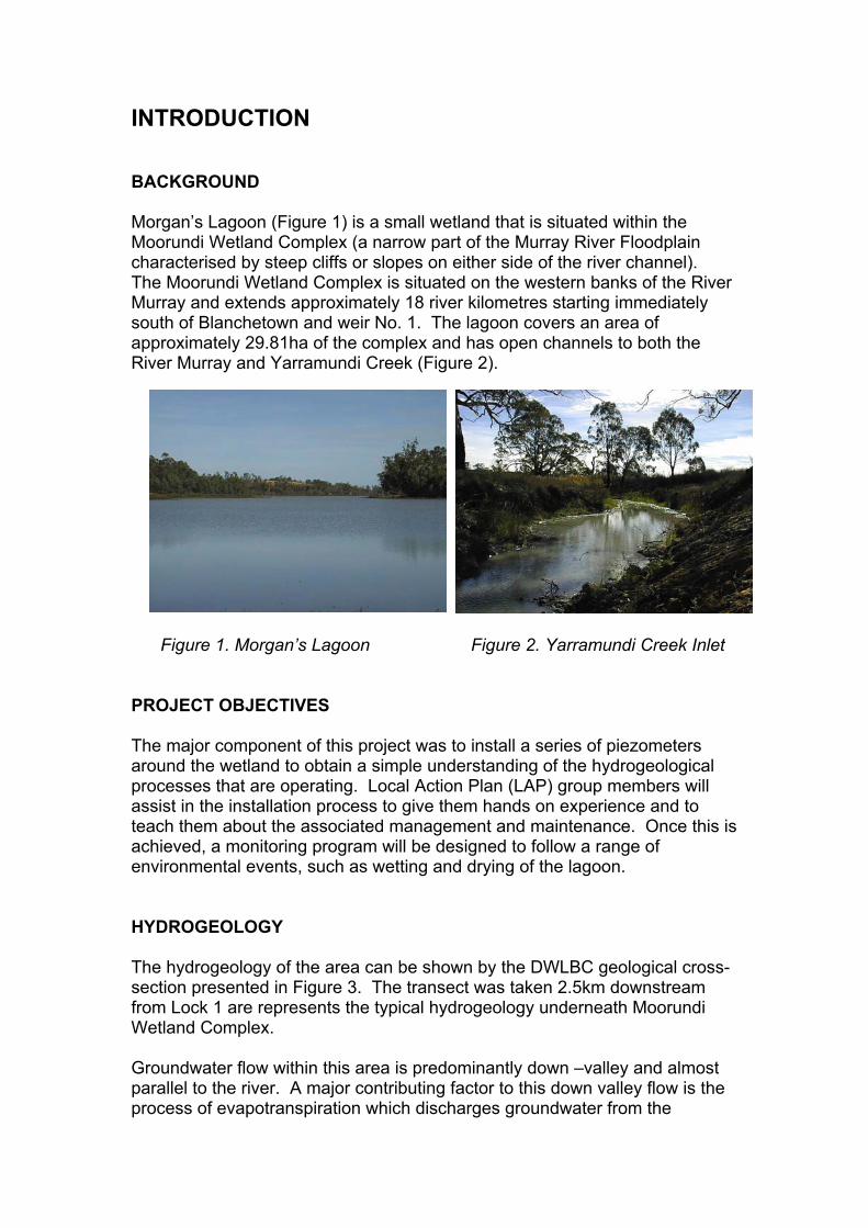
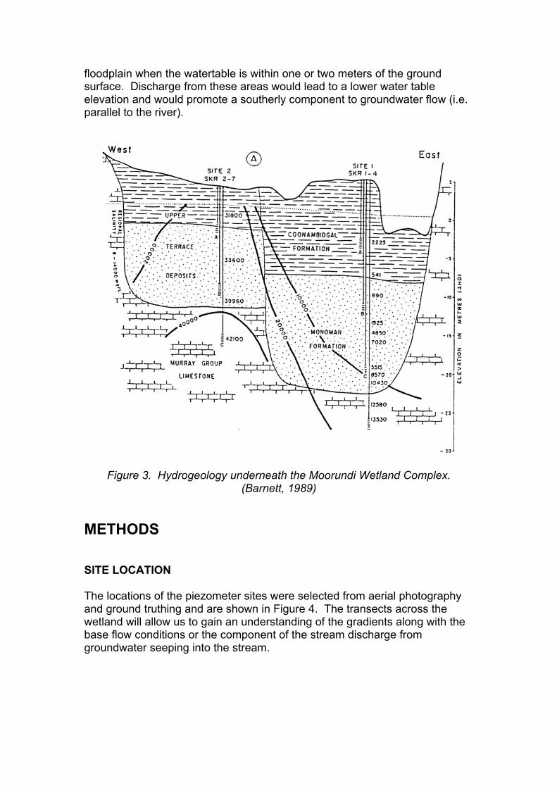
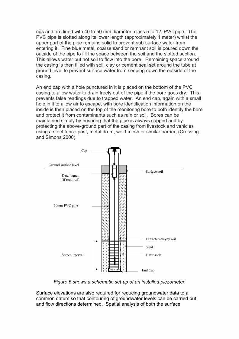
INTRODUCTION BACKGROUND Morgan’s Lagoon (Figure 1) is a small wetland that is situated within the Moorundi Wetland Complex (a narrow part of the Murray River Floodplain characterised by steep cliffs or slopes on either side of the river channel). The Moorundi Wetland Complex is situated on the western banks of the River Murray and extends approximately 18 river kilometres starting immediately south of Blanchetown and weir No. 1. The lagoon covers an area of approximately 29.81ha of the complex and has open channels to both the River Murray and Yarramundi Creek (Figure 2). Figure 1. Morgan’s Lagoon Figure 2. Yarramundi Creek Inlet PROJECT OBJECTIVES The major component of this project was to install a series of piezometers around the wetland to obtain a simple understanding of the hydrogeological processes that are operating. Local Action Plan (LAP) group members will assist in the installation process to give them hands on experience and to teach them about the associated management and maintenance. Once this is achieved, a monitoring program will be designed to follow a range of environmental events, such as wetting and drying of the lagoon. HYDROGEOLOGY The hydrogeology of the area can be shown by the DWLBC geological cross-section presented in Figure 3. The transect was taken 2.5km downstream from Lock 1 are represents the typical hydrogeology underneath Moorundi Wetland Complex. Groundwater flow within this area is predominantly down –valley and almost parallel to the river. A major contributing factor to this down valley flow is the process of evapotranspiration which discharges groundwater from the

floodplain when the watertable is within one or two meters of the ground surface. Discharge from these areas would lead to a lower water table elevation and would promote a southerly component to groundwater flow (i.e. parallel to the river).

Figure 3. Hydrogeology underneath the Moorundi Wetland Complex. (Barnett, 1989)

METHODS SITE LOCATION The locations of the piezometer sites were selected from aerial photography and ground truthing and are shown in Figure 4. The transects across the wetland will allow us to gain an understanding of the gradients along with the base flow conditions or the component of the stream discharge from groundwater seeping into the stream.

Figure 4. Location of the piezometers around Morgan’s Lagoon

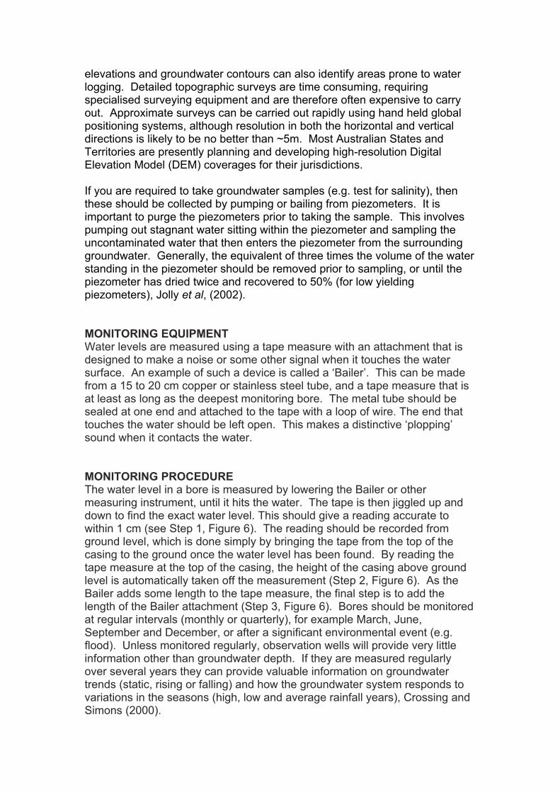
INSTALLATION OF GROUNDWATER MONITORING WELL/PIEZOMETERS Groundwater levels are measured using observation wells or piezometers (see Figure 5) and are generally drilled using rotary auger or rotary air blast

rigs and are lined with 40 to 50 mm diameter, class 5 to 12, PVC pipe. The PVC pipe is slotted along its lower length (approximately 1 meter) whilst the upper part of the pipe remains solid to prevent sub-surface water from entering it. Fine blue metal, coarse sand or remnant soil is poured down the outside of the pipe to fill the space between the soil and the slotted section. This allows water but not soil to flow into the bore. Remaining space around the casing is then filled with soil, clay or cement seal set around the tube at ground level to prevent surface water from seeping down the outside of the casing. An end cap with a hole punctured in it is placed on the bottom of the PVC casing to allow water to drain freely out of the pipe if the bore goes dry. This prevents false readings due to trapped water. An end cap, again with a small hole in it to allow air to escape, with bore identification information on the inside is then placed on the top of the monitoring bore to both identify the bore and protect it from contaminants such as rain or soil. Bores can be maintained simply by ensuring that the pipe is always capped and by protecting the above-ground part of the casing from livestock and vehicles using a steel fence post, metal drum, weld mesh or similar barrier, (Crossing and Simons 2000).

50mm

D(

S

Surface soil

Ground surface level

Cap

Figu Surface elevcommon datand flow dire

ata logger if required)

PVC pipe

creen interval

Sand

Extracted clayey soil

Filter sock

End Cap

re 5 shows a schematic set-up of an installed piezometer.

ations are also required for reducing groundwater data to a um so that contouring of groundwater levels can be carried out ctions determined. Spatial analysis of both the surface

elevations and groundwater contours can also identify areas prone to water logging. Detailed topographic surveys are time consuming, requiring specialised surveying equipment and are therefore often expensive to carry out. Approximate surveys can be carried out rapidly using hand held global positioning systems, although resolution in both the horizontal and vertical directions is likely to be no better than ~5m. Most Australian States and Territories are presently planning and developing high-resolution Digital Elevation Model (DEM) coverages for their jurisdictions. If you are required to take groundwater samples (e.g. test for salinity), then these should be collected by pumping or bailing from piezometers. It is important to purge the piezometers prior to taking the sample. This involves pumping out stagnant water sitting within the piezometer and sampling the uncontaminated water that then enters the piezometer from the surrounding groundwater. Generally, the equivalent of three times the volume of the water standing in the piezometer should be removed prior to sampling, or until the piezometer has dried twice and recovered to 50% (for low yielding piezometers), Jolly et al, (2002). MONITORING EQUIPMENT Water levels are measured using a tape measure with an attachment that is designed to make a noise or some other signal when it touches the water surface. An example of such a device is called a ‘Bailer’. This can be made from a 15 to 20 cm copper or stainless steel tube, and a tape measure that is at least as long as the deepest monitoring bore. The metal tube should be sealed at one end and attached to the tape with a loop of wire. The end that touches the water should be left open. This makes a distinctive ‘plopping’ sound when it contacts the water. MONITORING PROCEDURE The water level in a bore is measured by lowering the Bailer or other measuring instrument, until it hits the water. The tape is then jiggled up and down to find the exact water level. This should give a reading accurate to within 1 cm (see Step 1, Figure 6). The reading should be recorded from ground level, which is done simply by bringing the tape from the top of the casing to the ground once the water level has been found. By reading the tape measure at the top of the casing, the height of the casing above ground level is automatically taken off the measurement (Step 2, Figure 6). As the Bailer adds some length to the tape measure, the final step is to add the length of the Bailer attachment (Step 3, Figure 6). Bores should be monitored at regular intervals (monthly or quarterly), for example March, June, September and December, or after a significant environmental event (e.g. flood). Unless monitored regularly, observation wells will provide very little information other than groundwater depth. If they are measured regularly over several years they can provide valuable information on groundwater trends (static, rising or falling) and how the groundwater system responds to variations in the seasons (high, low and average rainfall years), Crossing and Simons (2000).

Figure 6. Diagram showing the monitoring procedure after Crossing and Simons (2000).

RESULTS Water table elevations shown in Table 1 were determined from dropping down an electronic water level meter in the installed piezometers. It should be noted that the obtained heights do not represent the hydraulic head as the aquifer as the site was not surveyed to the Australian Height Datum (AHD) or other known benchmark. Therefore, no conclusions can be made about the direction of the groundwater flow. However, after visiting the site it does seem that groundwater is moving away Morgan’s Lagoon and discharging into either the River Murray or Yarramundi Creek. It is also obvious that the water level in Morgan’s Lagoon was slightly higher than in the River Murray. It is believed that southerly winds push the water up Yarramundi Creek and into Morgan’s Lagoon. The main geology that was encountered whilst installing the piezometers was the Coonambidgal Formation, an alluvial grey to brown cracking clay. This has a tendency to act as a confining barrier to any surface recharge.

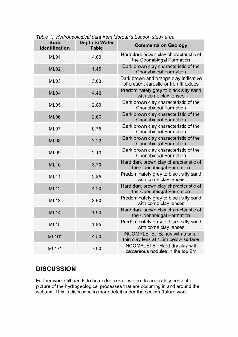
Table 1. Hydrogeological data from Morgan’s Lagoon study area

Bore Identification

Depth to Water Table Comments on Geology

ML01 4.00 Hard dark brown clay characteristic of the Coonabidgal Formation

ML02 1.45 Dark brown clay characteristic of the Coonabidgal Formation

ML03 3.03 Dark brown and orange clay indicative of present Jarosite or Iron III oxides

ML04 4.46 Predominately grey to black silty sand with come clay lenses












ML16* 4.50 INCOMPLETE. Sandy with a small thin clay lens at 1.5m below surface

ML17* 7.00 INCOMPLETE. Hard dry clay with calcareous nodules in the top 2m

DISCUSSION Further work still needs to be undertaken if we are to accurately present a picture of the hydrogeological processes that are occurring in and around the wetland. This is discussed in more detail under the section “future work”.

MONITORING Records of groundwater depth are most useful for assessing risk when sufficiently long and frequent data are available. When interpreting groundwater data it is important to be aware that water tables can fluctuate at a range of temporal scales. For example they can be episodic in response to very large rainfall events, fluctuate due to varying climatic conditions, or can exhibit long-term water table rise or fall in response to land use changes. They can also demonstrate various combinations of these behaviours. In order to account for seasonal and episodic variation in groundwater levels and establish long-term trends, it is necessary to monitor water table depths on at least a monthly basis. It is also important to be aware that in many situations rising water tables are driven by increasing pressures in underlying semi-confined and confined aquifers, and so installation of piezometers at multiple depths at a site is often required. Also of importance is to interpret the data in the context of the groundwater flow systems they are monitoring. Tools such as FLOWTUBE (Dawes et al., 2000) can assist in reviewing and interpreting groundwater level data in this context. Groundwater salinities generally fluctuate much less than water table levels and so annual measurements are usually sufficient. LONG TERM MONITORING To detect whether the watertable is rising, falling or is, stationary over a period of years, check watertable depths regularly and record or graph them in the farm office. The most suitable time for measuring depths is in October, when the risk of capillary rise is greatest. A measurement in April should give the deepest watertable readings and one in August the shallowest depth to water. Annual checking of the vegetation boundary will also indicate whether the salt land problem is getting worse or is stable. Regular soil sampling near the holes, every three years or so, will also confirm any changes in the soil salinity suggested by the vegetation. Take the samples at the same time of year in mid-summer, but not within three weeks of heavy rain. You have evidence of a worsening situation and of its rate of change, if, over a period of years:

• the watertable levels in spring and summer are rising; • the clover/barley grass boundary is moving outwards; and • topsoil salinity levels are increasing.

However, you have evidence of a stable situation under the present climatic and management regime, if the watertable levels, vegetation boundaries and topsoil salinities are not changing. Adopting this monitoring system win enable you to concentrate your concern and action where salt encroachment is most significant.

MANAGEMENT Goal setting, while seemingly obvious, this is the most important step in the management process. With very few exceptions, it will not be possible to completely restore a native vegetation community back to its natural condition. Cramer and Hobbs (2002) highlight the need to set priorities for the protection and restoration of native vegetation at risk based on an assessment of relative threat and probability of persistence or recovery. It is therefore important to clearly identify what is achievable for a given situation. Management goals can be summarised into three main categories: (i) recovery of the ecosystem; (ii) containment of further impacts; and (iii) adaptation to the new salinity regime. The decision will be based on the financial and technical resources available, ecological significance of the area and its current health, stakeholder aspirations, and other considerations. In most instances tradeoffs will be needed. FUTURE WORK The following is a recommendation list only;

• Surveying the area to AHD to obtain actual hydraulic heads. It may be feasible to investigate whether a high-resolution Digital Elevation Model covers the area. Heights obtained from a Global Positioning Systems (GPS) have a fairly low resolution (~5) and considering that the land in this area is relatively flat, a detailed topographic survey might be a better option.

• Use a numerical groundwater model such as MODFLOW or

FLOWTUBE to assist in reviewing and interpreting groundwater level data. This would increase the understanding of the hydrogeology within this part of the Moorundi Wetland Complex and hence, allow us to potentially transfer management practices to other parts of the complex.

REFERENCES Barnett, S. R., (1989). The hydrogeology of the Murray Basin in South Australia with special reference to the alluvium of the River Murray floodplain. Unpublished M.Sc. Thesis, Flinders University of South Australia. Cramer, V.A. and Hobbs, R.J. (2002). Ecological consequences of altered hydrological regimes in fragmented ecosystems in southern Australia: impacts and possible management responses. Austral Ecology (in press). Crossing, L. and Simons, J. (2000). Monitoring Groundwater Levels. Farmnote. Agriculture Western Australia, Perth.

Dawes, W.R., Stauffacher, M. and Walker, G.R. (2000). Calibration and modelling of groundwater processes in the Liverpool Plains, CSIRO Land and Water Technical Report 05/2000 Jensen, A., and Turner, R. (2002). Moorundi Wetland Complex Management Plan. Report for the Mid Murray Local Action Plan Association. Jolly, I., McEwan, K., Cox, J., Walker, G., and Holland, K., (2002). Managing Groundwater and Surface Water for Native Terrestrial Vegetation Health in Saline Areas. CSIRO Land and Water Technical Report 23/02

moorundi wetlands groundwater monitoring network

Documents