more-advanced statistical sampling concepts for...

Fourth Pass

smi87468_app10B_10B1-10B67 10B-1 09/15/15 07:17 PM

A P P E N D I X 1 0 B

More-Advanced Statistical Sampling Concepts for Tests of Controls and Tests of BalancesAppendix 10B contains more mathematical and statistical details related to the test of controls sampling introduced in Chapter 10. In fact, it is like a technical appendix on test of controls sampling and substantive testing. In this appendix you will find more-specific explanations of how to do statistical sampling in the test of controls phase of the control risk assessment work, and for substantive tests of details. After studying this appendix in conjunction with Chapter 10, you should be familiar with and able to perform the listed topic items.

LO8 Demonstrate that you can apply statistical sampling concepts for tests of controls and tests of balances

using the audit risk model.

Appendix TopicsPart I: Some More Theory on the Behaviour of Sampling Risks

Part II: Test of Controls with Attribute Sampling Risk and Rate Quantifications

• Explain how risks behave under the hypothesis testing approach in statistical sampling. • Explain the role of professional judgment in assigning numbers to risk of assessing control risk too

low, risk of assessing control risk too high (efficiency risk), and tolerable deviation rate. • Use statistical tables or calculations to determine test of controls sample sizes when there is more than

one population. • Use tables and calculations to compute statistical results (the computed upper error limit (UEL), which

is the same as achieved P in Chapter 10) for evidence obtained with detail test of controls procedures. • Use the discovery sampling evaluation table for assessment of audit evidence. • Choose a test of controls sample size from among several equally acceptable alternatives.

10B-1

Fourth Pass

10B-2 PART 2 Basic Auditing Concepts and Techniques

smi87468_app10B_10B1-10B67 10B-2 09/15/15 07:17 PM

Part III: Audit of an Account Balance • Calculate a risk of incorrect acceptance, given judgments about inherent risk, control risk, and ana-

lytical procedures risk, using the audit risk model, such as in the CPA Canada Handbook Section 5095, Guideline on Materiality (AuG-41, paragraphs 41 and 42).

• Explain the considerations in controlling the risk of incorrect rejection. • Explain the characteristics of monetary-unit sampling (MUS) and its relationship to attribute sampling. • Calculate a monetary-unit sample size for the audit of the details of an account balance. • Describe a method for selecting a monetary unit, define a logical unit, and explain the stratification

effect of MUS. • Calculate a UEL for the evaluation of monetary-value evidence, and discuss the relative merits of

alternatives for determining an amount by which a monetary balance should be adjusted. • Use your critical thinking skills to evaluate newspaper articles about auditor applications of statistical

sampling.

Part IV: Other Topics in Statistical Auditing: Regression for Analytical Review, Monetary-Unit Sampling for Tests of Controls, and the Audit Risk Model

• Explain how linear regression can be used as an analytical review procedure. • Describe the advantages of using MUS to test controls. • Explain how the audit risk model evolved from the adoption of statistical sampling in auditing.

Part I: Some More Theory on the Behaviour of Sampling Risks This appendix continues the discussion that began in Chapter 10 regarding statistical sampling in auditing. As you will recall, Chapter 10 ends with some of the mechanics of using statistical formulas and tables in auditing. Here, in this appendix, you will find more details on the theory and mechanics of statistical audit-ing. We begin with an overview of some theory about how risks are controlled with all statistical audit pro-cedures, using the concept of hypothesis testing. We then review applications to attribute sampling in tests of controls, followed by statistical applications of substantive testing of details on balances. The appendix ends with statistical applications of regression models to analytical review procedures.

Under the negative approach, confidence level equals one minus effectiveness risk, while under the positive approach, confidence level equals one minus efficiency risk.

Recall that the negative approach is the more important and common approach in auditing. In particular, it underlies all attribute sampling tables and formulas. MUS always uses the negative approach. The positive approach frequently underlies formulas using the normal distribution assumption; this is briefly discussed at the end of the appendix. Because of its simplicity and straightforward relationship to audit objectives, the negative approach is used throughout the appendix. However, it should be noted that the positive approach is much more important in the sciences, and, in particular, the efficiency risk when associated with the null hypothesis of “no difference” is the more important risk of the sciences. In contrast, the effectiveness or effectiveness risk is more important in auditing because it is related to the more important hypothesis of “material misstatement” or “significant difference,” which it is the auditor’s job to detect. In fact, some have characterized the purpose of the auditing profession as “controlling effectiveness risk” associated with financial statements. For this reason, effectiveness risk is associated with audit effectiveness.

Fourth Pass

APPENDIX 10B More-Advanced Statistical Sampling Concepts for Tests of Controls and Tests of Balances 10B-3

smi87468_app10B_10B1-10B67 10B-3 09/15/15 07:17 PM

How Sampling Risks Are Controlled in Statistical AuditingWhen using statistical sampling concepts in auditing, we need to develop a decision rule, which must be used consistently if we are to control risks objectively. It is the assumption of the consistent use of a strict decision rule that allows the risks to be predicted and thus controlled via the sample size. The decision rule is frequently referred to as a hypothesis test, and the auditor is typically interested in distinguishing between two hypotheses:

Hypothesis 1: There exists a material misstatement in the total amount recorded for the accounting population.

Hypothesis 2: There exists no misstatement in the amount recorded for the accounting population.

The decision rule the auditor uses in statistical auditing is to select one of these two hypotheses based on the results of the statistical sample. The mechanics of this will be discussed later in this appendix. For now, we are interested in depicting what happens to sampling risks (risks that arise when testing only a portion of the population statistically) when a consistent decision rule is used. This is when the summary concept of a probability of acceptance curve becomes useful. This curve can be used to represent all the possibili-ties of sampling risk about a sample result.

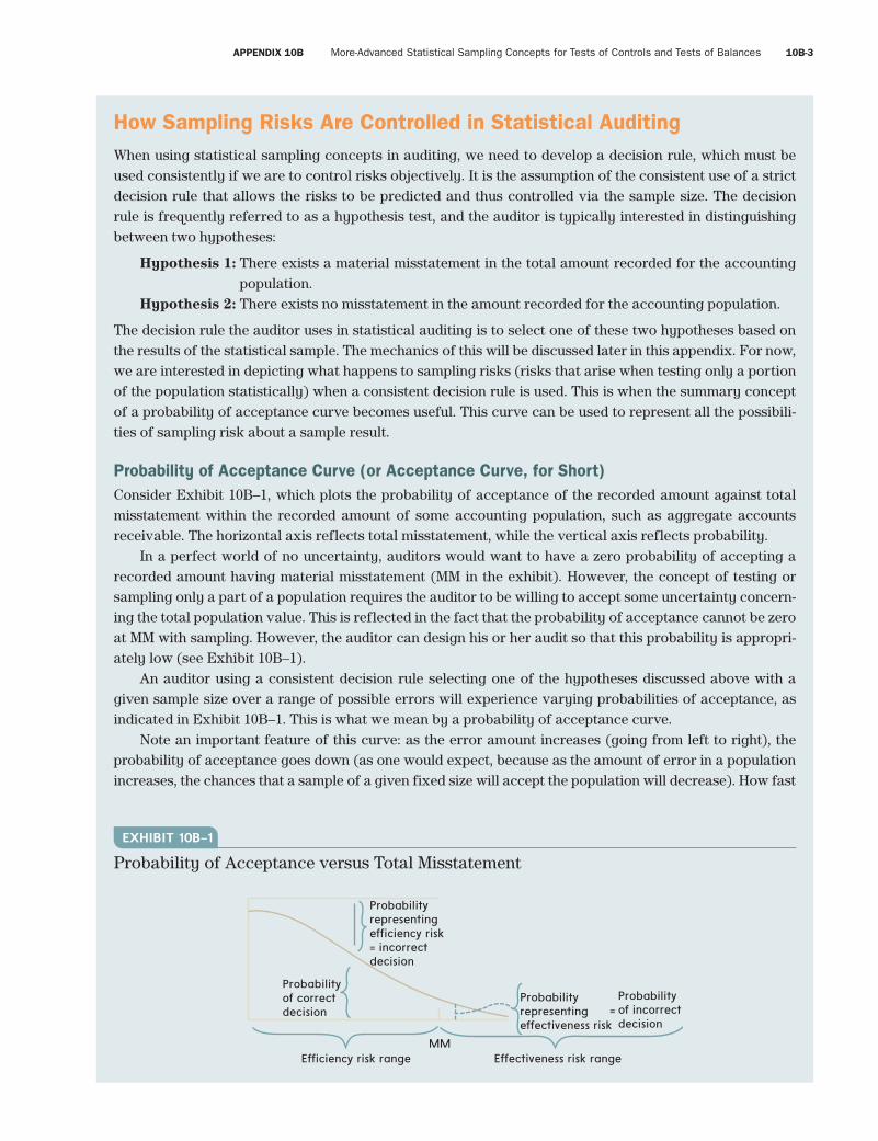
Probability of Acceptance Curve (or Acceptance Curve, for Short)Consider Exhibit 10B–1, which plots the probability of acceptance of the recorded amount against total misstatement within the recorded amount of some accounting population, such as aggregate accounts receivable. The horizontal axis reflects total misstatement, while the vertical axis reflects probability.

In a perfect world of no uncertainty, auditors would want to have a zero probability of accepting a recorded amount having material misstatement (MM in the exhibit). However, the concept of testing or sampling only a part of a population requires the auditor to be willing to accept some uncertainty concern-ing the total population value. This is reflected in the fact that the probability of acceptance cannot be zero at MM with sampling. However, the auditor can design his or her audit so that this probability is appropri-ately low (see Exhibit 10B–1).

An auditor using a consistent decision rule selecting one of the hypotheses discussed above with a given sample size over a range of possible errors will experience varying probabilities of acceptance, as indicated in Exhibit 10B–1. This is what we mean by a probability of acceptance curve.

Note an important feature of this curve: as the error amount increases (going from left to right), the probability of acceptance goes down (as one would expect, because as the amount of error in a population increases, the chances that a sample of a given fixed size will accept the population will decrease). How fast

Probabilityrepresentingefficiency risk= incorrectdecision

Probabilityrepresentingeffectiveness risk

Probabilityof correctdecision

MMEfficiency risk range Effectiveness risk range

Probabilityof incorrectdecision

=

EXHIBIT 10B–1

Probability of Acceptance versus Total Misstatement

Fourth Pass


smi87468_app10B_10B1-10B67 10B-4 09/15/15 07:17 PM

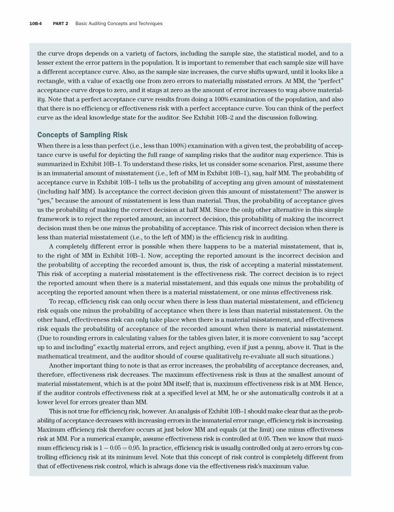
the curve drops depends on a variety of factors, including the sample size, the statistical model, and to a lesser extent the error pattern in the population. It is important to remember that each sample size will have a different acceptance curve. Also, as the sample size increases, the curve shifts upward, until it looks like a rectangle, with a value of exactly one from zero errors to materially misstated errors. At MM, the “perfect” acceptance curve drops to zero, and it stays at zero as the amount of error increases to way above material-ity. Note that a perfect acceptance curve results from doing a 100% examination of the population, and also that there is no efficiency or effectiveness risk with a perfect acceptance curve. You can think of the perfect curve as the ideal knowledge state for the auditor. See Exhibit 10B–2 and the discussion following.

Concepts of Sampling RiskWhen there is a less than perfect (i.e., less than 100%) examination with a given test, the probability of accep-tance curve is useful for depicting the full range of sampling risks that the auditor may experience. This is summarized in Exhibit 10B–1. To understand these risks, let us consider some scenarios. First, assume there is an immaterial amount of misstatement (i.e., left of MM in Exhibit 10B–1), say, half MM. The probability of acceptance curve in Exhibit 10B–1 tells us the probability of accepting any given amount of misstatement (including half MM). Is acceptance the correct decision given this amount of misstatement? The answer is “yes,” because the amount of misstatement is less than material. Thus, the probability of acceptance gives us the probability of making the correct decision at half MM. Since the only other alternative in this simple framework is to reject the reported amount, an incorrect decision, this probability of making the incorrect decision must then be one minus the probability of acceptance. This risk of incorrect decision when there is less than material misstatement (i.e., to the left of MM) is the efficiency risk in auditing.

A completely different error is possible when there happens to be a material misstatement, that is, to the right of MM in Exhibit 10B–1. Now, accepting the reported amount is the incorrect decision and the probability of accepting the recorded amount is, thus, the risk of accepting a material misstatement. This risk of accepting a material misstatement is the effectiveness risk. The correct decision is to reject the reported amount when there is a material misstatement, and this equals one minus the probability of accepting the reported amount when there is a material misstatement, or one minus effectiveness risk.

To recap, efficiency risk can only occur when there is less than material misstatement, and efficiency risk equals one minus the probability of acceptance when there is less than material misstatement. On the other hand, effectiveness risk can only take place when there is a material misstatement, and effectiveness risk equals the probability of acceptance of the recorded amount when there is material misstatement. (Due to rounding errors in calculating values for the tables given later, it is more convenient to say “accept up to and including” exactly material errors, and reject anything, even if just a penny, above it. That is the mathematical treatment, and the auditor should of course qualitatively re-evaluate all such situations.)

Another important thing to note is that as error increases, the probability of acceptance decreases, and, therefore, effectiveness risk decreases. The maximum effectiveness risk is thus at the smallest amount of material misstatement, which is at the point MM itself; that is, maximum effectiveness risk is at MM. Hence, if the auditor controls effectiveness risk at a specified level at MM, he or she automatically controls it at a lower level for errors greater than MM.

This is not true for efficiency risk, however. An analysis of Exhibit 10B–1 should make clear that as the prob-ability of acceptance decreases with increasing errors in the immaterial error range, efficiency risk is increasing. Maximum efficiency risk therefore occurs at just below MM and equals (at the limit) one minus effectiveness risk at MM. For a numerical example, assume effectiveness risk is controlled at 0.05. Then we know that maxi-mum efficiency risk is 1 − 0.05 = 0.95. In practice, efficiency risk is usually controlled only at zero errors by con-trolling efficiency risk at its minimum level. Note that this concept of risk control is completely different from that of effectiveness risk control, which is always done via the effectiveness risk’s maximum value.

Fourth Pass


smi87468_app10B_10B1-10B67 10B-5 09/15/15 07:17 PM

The difference between behaviours of the two sampling risks and the different concepts of control of efficiency and effectiveness risks have important implications for auditors. First, note that it is a very good thing that we can control effectiveness risk at its maximum! This is because effectiveness risk is the more important risk for auditors. It is so important that some people characterize the reason for the existence of the audit profession as being to control effectiveness risk. If auditors do not detect material misstatements in financial statements, then who will? Thus, effectiveness risk can be said to relate to audit effectiveness.

Note also that effectiveness risk is very treacherous. This is so because the auditor has no idea that an effectiveness-type incorrect decision is being made. The sample evidence gives no indication that the amount of misstatement is material. The only way to control effectiveness risk is by planning for it in advance during the sample planning stage of the audit. In statistical sampling formulas, this is done through the calculation of the sample size using a planned precision for the test, similar to the polling example discussed in the chapter. More illustrations will be provided later in this appendix.

The consequences of an efficiency-type error are much less dire for the auditor but could be important nevertheless. The auditor is aware that there may be a problem because by rejecting a sample result, there is either a material misstatement or an efficiency error. At this point, auditors have several options: (a) review evidence of related tests, (b) expand audit work by increasing the sample size of the test and related procedures (the audit risk model can assist in this task), (c) ask for an adjustment of the recorded amount of the population so that the estimated probability of material misstatement is reduced to an acceptable amount, or (d) perhaps modify the audit opinion based on the test results. The appropriate action, again, depends on professional judgment and the circumstances. The auditor should, however, be prepared to give good reasons for the decision. Generally, an efficiency-type incorrect decision increases the amount of audit work unnecessarily, and thus it is characterized as an audit efficiency error. There is more com-plete discussion of auditor options at various stages of the audit later in the appendix.

Positive and Negative Approaches and Confidence LevelIn the statistical literature, there is frequent reference to the concept of the confidence level of a statistical test. How does this relate to efficiency and effectiveness risks as used in auditing? The answer depends on a number of things, such as the way the hypothesis tests are constructed. Confidence level is related to the primary or null hypothesis of the test. Specifically, confidence level equals one minus the risk of rejecting the null hypothesis when it is true. Thus, confidence level depends on the null hypothesis used. In auditing, a distinctive statistical terminology has evolved over the years: if hypothesis 1 is the null hypothesis, then we are using the negative approach to hypothesis testing, and if hypothesis 2 is the null hypothesis, then we are using the positive approach to hypothesis testing. Under the negative approach, confidence level equals one minus effectiveness risk, while under the positive approach, confidence level equals one minus efficiency risk.

The negative approach is the more important and common approach in auditing. Most important is that the effectiveness risk is controlled by selecting the appropriate confidence level, since confidence level equals one minus effectiveness risk. This also means that the confidence level is aligned with the assurance level provided by the test. This can be seen by noting that effectiveness risk is very similar to the definitions of the audit risk model and its various component risks. This aspect of the audit risk model is further discussed in the Application Case for this appendix. The negative approach is normally used to statistically test inter-nal controls. In particular, it underlies all attribute sampling tables and formulas. MUS, discussed later in the appendix, always uses the negative approach.

On the other hand, the positive approach frequently underlies formulas using the normal distribution assumption. The consequences of this are briefly discussed at the end of the appendix. Because of its simplicity and straightforward relationship to audit objectives, the negative approach is used throughout the remain-der of the appendix. However, it should be noted that the positive approach is much more important in the

Fourth Pass


smi87468_app10B_10B1-10B67 10B-6 09/15/15 07:17 PM

sciences, and, in particular, the efficiency risk, when associated with the null hypothesis of “no difference,” is the more important risk of the sciences. Thus, your statistics course may have used a positive approach, and so within that course confidence level equals one minus efficiency risk. Under the positive approach, there is a less-straightforward relationship between assurance, as the auditor uses that term, and the con-fidence level. Hence, under the positive approach the auditor needs to make adjustments to the confidence level in determining the assurance level provided by the statistical test. These adjustments are particularly important if the statistical test is to be used with the audit risk model.

If we use the negative approach, then the effectiveness risk is controlled directly through the confidence level, as discussed above. But then, how is efficiency risk controlled using the negative approach? The first thing to remember is that efficiency risk cannot be “controlled” the same way that effectiveness risk is con-trolled (at effectiveness risk’s maximum level). As discussed above, you can only “control” efficiency risk at its minimum value. This is true regardless of whether the positive or negative approach is used. With the formulas we use, this minimum efficiency risk is zero. Under the negative approach, the way to reduce effi-ciency risk throughout its range is to use a sample size that is bigger than the minimum for the confidence level of the test. Remember that under the negative approach, confidence level equals one minus effective-ness risk, so you are already controlling effectiveness risk once you set the confidence level. Any audit plan that wants to reduce efficiency risk across the entire efficiency risk range needs to do so by increasing the sample size beyond that of the minimum for the stated confidence level. This is illustrated in the end-of-appendix discussion case and discussed in more detail later in this appendix.

Effect of Changing the Sample Size under the Negative ApproachUnder the negative approach, confidence level (CL) = 1 − effectiveness risk. Under some interpretations, auditors can equate the confidence level with audit assurance, and so these auditors work with assurance or confidence factors rather than risk factors. The underlying principles remain essentially the same, how-ever, whether the auditor works with risk or confidence levels.

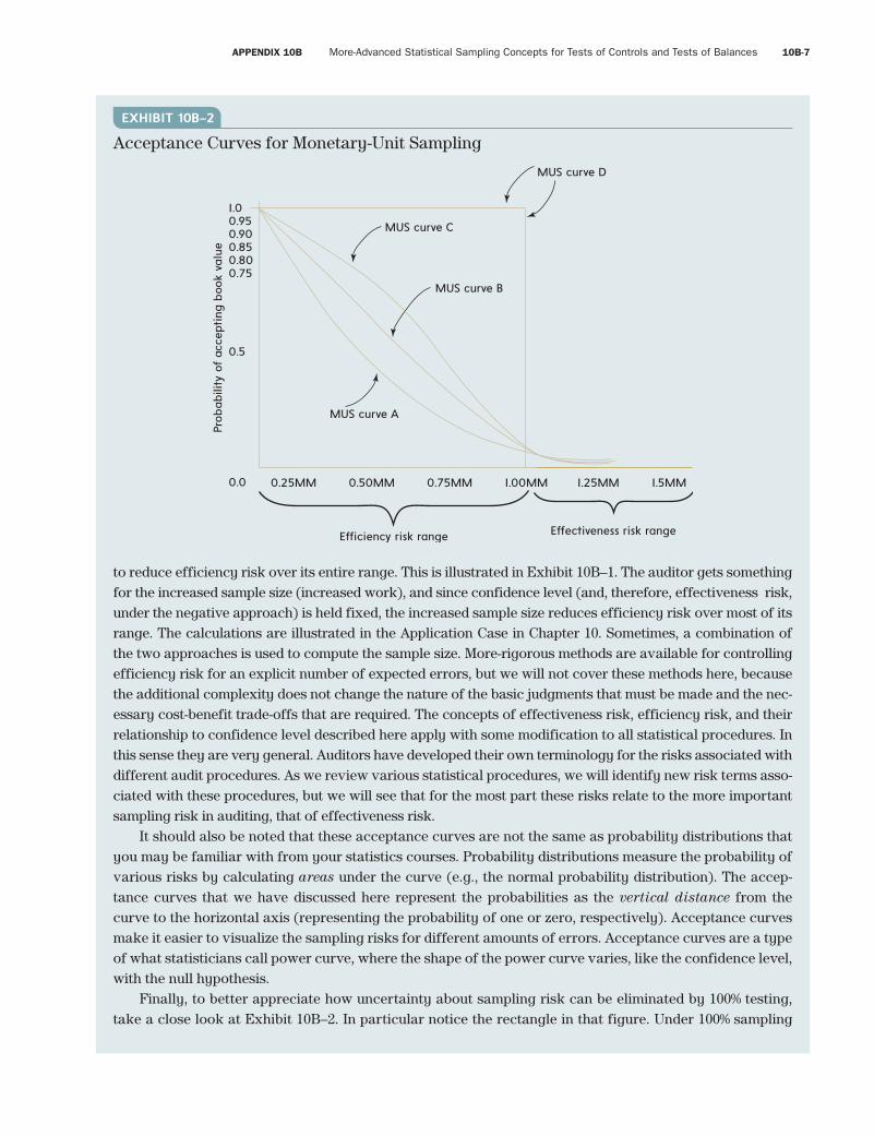
What if the auditor varies the sample size while keeping the confidence level constant?Exhibit 10B–2 illustrates what happens: curve A is the probability of acceptance with the smallest sample

size possible for given effectiveness risk, curve B results from using twice the curve A sample size, and curve C results from four times the curve A sample size, whereas curve D represents a “perfect acceptance curve” with no sampling risk. Curve D occurs when a population is examined 100%. From Exhibit 10B–2, it is evident that if confidence level (and thus effectiveness risk, under the negative approach) and material misstatement (MM) are held constant while changing the sample size, it is the efficiency risk that changes with the sample size—specifically, efficiency risk is reduced throughout its range when the sample size is increased, and vice versa. This illustrates that if the auditor wishes to reduce efficiency risk while keeping effectiveness risk and MM unchanged, then a larger sample size needs to be used. In fact, if any one of efficiency risk, effectiveness risk, and MM were to be reduced, sample size would need to be increased, and vice versa.

Curve A reflects the acceptance curve with the smallest sample size possible with MUS for a given effec-tiveness risk (1 – CL). This smallest sample size is called a discovery sample. If the auditor wishes to control efficiency risk to a lower level than indicated by curve A, the sample size should be increased, while keep-ing the planned precision and confidence level fixed. Sample size increases in practice are normally imple-mented through formulas by one of two major approaches: (1) increase the number of errors to be accepted by the sample, or (2) increase the planned expected error rate in computing the sample size. The second approach is the one suggested in CAS 530. This approach also helps explain the concept of performance materiality in Chapter 5 and CAS 530. If the smaller performance materiality is used in planning a sample size but the overall (or specific) materiality of Chapter 5 is used to evaluate the sample results, then the effect is

Fourth Pass


smi87468_app10B_10B1-10B67 10B-7 09/15/15 07:17 PM

to reduce efficiency risk over its entire range. This is illustrated in Exhibit 10B–1. The auditor gets something for the increased sample size (increased work), and since confidence level (and, therefore, effectiveness risk, under the negative approach) is held fixed, the increased sample size reduces efficiency risk over most of its range. The calculations are illustrated in the Application Case in Chapter 10. Sometimes, a combination of the two approaches is used to compute the sample size. More-rigorous methods are available for controlling efficiency risk for an explicit number of expected errors, but we will not cover these methods here, because the additional complexity does not change the nature of the basic judgments that must be made and the nec-essary cost-benefit trade-offs that are required. The concepts of effectiveness risk, efficiency risk, and their relationship to confidence level described here apply with some modification to all statistical procedures. In this sense they are very general. Auditors have developed their own terminology for the risks associated with different audit procedures. As we review various statistical procedures, we will identify new risk terms asso-ciated with these procedures, but we will see that for the most part these risks relate to the more important sampling risk in auditing, that of effectiveness risk.

It should also be noted that these acceptance curves are not the same as probability distributions that you may be familiar with from your statistics courses. Probability distributions measure the probability of various risks by calculating areas under the curve (e.g., the normal probability distribution). The accep-tance curves that we have discussed here represent the probabilities as the vertical distance from the curve to the horizontal axis (representing the probability of one or zero, respectively). Acceptance curves make it easier to visualize the sampling risks for different amounts of errors. Acceptance curves are a type of what statisticians call power curve, where the shape of the power curve varies, like the confidence level, with the null hypothesis.

Finally, to better appreciate how uncertainty about sampling risk can be eliminated by 100% testing, take a close look at Exhibit 10B–2. In particular notice the rectangle in that figure. Under 100% sampling

EXHIBIT 10B–2

Acceptance Curves for Monetary-Unit Sampling

MUS curve D

MUS curve C

MUS curve B

MUS curve A

1.00.950.900.850.800.75

0.5

0.0

Probabili

ty o

f ac

cept

ing b

ook

valu

e

Efficiency risk range Effectiveness risk range

0.50MM 0.25MM 0.75MM 1.00MM 1.5MM1.25MM

Fourth Pass


smi87468_app10B_10B1-10B67 10B-8 09/15/15 07:17 PM

the vertical part of the rectangle drops at exactly 1.00MM. This mean that even one penny above MM the probability of acceptance drops to zero, meaning the effectiveness risk is zero at MM. The rectangle also means that just to the left of (i.e., below) MM the probability of acceptance is exactly one (meaning there is no efficiency risk). Thus, with no sampling risk the auditor always accepts the recorded amount at or below MM and rejects just above MM. In other words, the auditor can perfectly distinguish between the material and immaterial amount of error with 100% testing. This is something one would expect with per-fect knowledge of the population.

But, logically, the perfect rectangular acceptance curve occurs only with the negative testing approach to hypothesis testing. Under the positive approach to hypothesis testing, perfect knowledge represented by 100% testing would mean the auditor accepts only the zero errors null hypothesis and rejects all non-zero errors. This follows from the different logics underlying the two testing approaches and illustrates that the negative approach is more consistent with the logic of auditing.

Part II: Test of Controls with Attribute Sampling Risk and Rate QuantificationsThe quantification of sampling risk is an exercise of professional judgment. When using statistical sam-pling methods, auditors must quantify the two risks of decision error. The risk of assessing control risk too low is generally considered more important than the risk of assessing control risk too high. Auditors must also exercise professional judgment to determine the extent of deviation allowable (tolerable rate) in assessing control risk.

Tolerable Deviation Rate: A Professional JudgmentAuditors should have an idea about the correspondence of rates of deviation in the population with control risk assessments. Perfect control compliance is not necessary, so the question is what rate of deviation in the population signals control risk of 10%, 20%, or 30%, and so forth, up to 100%? To answer this question, you need to relate material misstatement of an account to a tolerable deviation rate for the control proce-dures affecting that account.

Assume that a material dollar misstatement of $30,000 is used in planning the audit of accounts receiv-able for possible overstatement. This amount is relevant to the audit of control over sales transactions because uncorrected errors in sales transactions misstate the financial statements by remaining uncor-rected in the accounts receivable balance. In other words, we test the controls over sales transaction pro-cessing in order to determine the control risk relevant to our audit of the accounts receivable balance. Therefore, if sales transactions are in error by $30,000 or more, the accounts receivable balance may be materially misstated.

However, a deviation in a sales transaction (e.g., one unsupported by shipping documents) does not necessarily mean the transaction amount is totally in error. After all, missing paperwork may be the only problem. Perhaps a better example is a mathematical accuracy deviation; if a sales invoice is computed incorrectly to charge the customer $2,000 instead of $1,800, there is a 100% control deviation (the inaccu-racy), but it does not describe a 100% dollar error. Therefore, more than $30,000 in sales transactions can be “exposed” to control deviation without generating a $30,000 error in the sales and the accounts receiv-able balances. This “exposure” is sometimes called the smoke/fire concept, meaning that there can be more exposure to error (smoke) than actual error (fire), just as in a conflagration.

Fourth Pass


smi87468_app10B_10B1-10B67 10B-9 09/15/15 07:17 PM

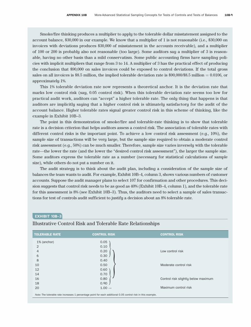
Smoke/fire thinking produces a multiplier to apply to the tolerable dollar misstatement assigned to the account balance, $30,000 in our example. We know that a multiplier of 1 is not reasonable (i.e., $30,000 on invoices with deviations produces $30,000 of misstatement in the accounts receivable), and a multiplier of 100 or 200 is probably also not reasonable (too large). Some auditors say a multiplier of 3 is reason-able, having no other basis than a mild conservatism. Some public accounting firms have sampling poli-cies with implicit multipliers that range from 3 to 14. A multiplier of 3 has the practical effect of producing the conclusion that $90,000 on sales invoices could be exposed to control deviations. If the total gross sales on all invoices is $8.5 million, the implied tolerable deviation rate is $90,000/$8.5 million = 0.0106, or approximately 1%.

This 1% tolerable deviation rate now represents a theoretical anchor. It is the deviation rate that marks low control risk (say, 0.05 control risk). When this tolerable deviation rate seems too low for practical audit work, auditors can “accept” a higher tolerable rate. The only thing that happens is that auditors are implicitly saying that a higher control risk is ultimately satisfactory for the audit of the account balance. Higher tolerable rates signal greater control risk in this scheme of thinking, like the example in Exhibit 10B–3.

The point in this demonstration of smoke/fire and tolerable-rate thinking is to show that tolerable rate is a decision criterion that helps auditors assess a control risk. The association of tolerable rates with different control risks is the important point. To achieve a low control risk assessment (e.g., 10%), the sample size of transactions will be very large, but the sample size required to obtain a moderate control risk assessment (e.g., 50%) can be much smaller. Therefore, sample size varies inversely with the tolerable rate—the lower the rate (and the lower the “desired control risk assessment”), the larger the sample size. Some auditors express the tolerable rate as a number (necessary for statistical calculations of sample size), while others do not put a number on it.

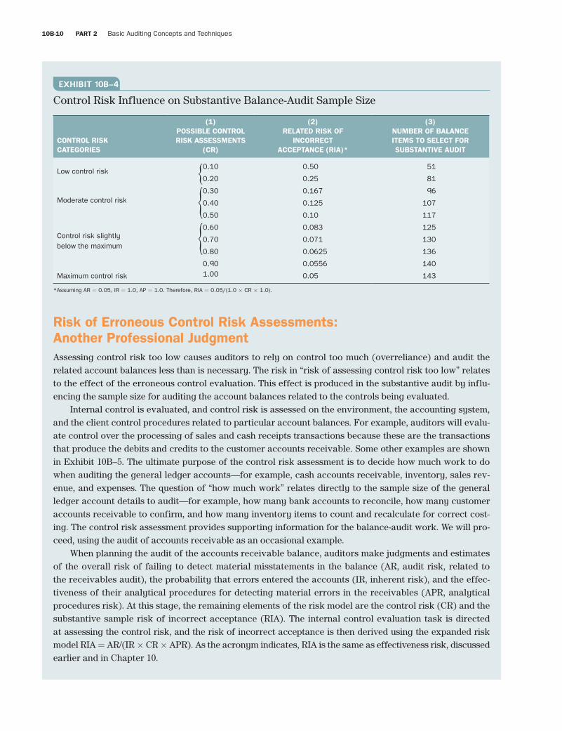
The audit strategy is to think about the audit plan, including a consideration of the sample size of balances the team wants to audit. For example, Exhibit 10B–4, column 3, shows various numbers of customer accounts. Suppose the audit manager plans to select 107 for confirmation and other procedures. This deci-sion suggests that control risk needs to be as good as 40% (Exhibit 10B–4, column 1), and the tolerable rate for this assessment is 8% (see Exhibit 10B–3). Thus, the auditors need to select a sample of sales transac-tions for test of controls audit sufficient to justify a decision about an 8% tolerable rate.

EXHIBIT 10B–3

Illustrative Control Risk and Tolerable Rate Relationships

TOLERABLE RATE CONTROL RISK CONTROL RISK

1% (anchor) 2 4 6 8101214161820

0.050.100.200.300.400.500.600.700.800.901.00 →

Low control risk

Moderate control risk

Control risk slightly below maximum

Maximum control risk

Note: The tolerable rate increases 1 percentage point for each additional 0.05 control risk in this example.

Fourth Pass


smi87468_app10B_10B1-10B67 10B-10 09/15/15 07:17 PM

Risk of Erroneous Control Risk Assessments: Another Professional JudgmentAssessing control risk too low causes auditors to rely on control too much (overreliance) and audit the related account balances less than is necessary. The risk in “risk of assessing control risk too low” relates to the effect of the erroneous control evaluation. This effect is produced in the substantive audit by influ-encing the sample size for auditing the account balances related to the controls being evaluated.

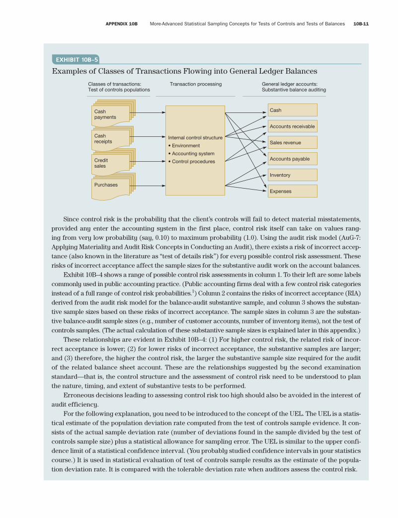
Internal control is evaluated, and control risk is assessed on the environment, the accounting system, and the client control procedures related to particular account balances. For example, auditors will evalu-ate control over the processing of sales and cash receipts transactions because these are the transactions that produce the debits and credits to the customer accounts receivable. Some other examples are shown in Exhibit 10B–5. The ultimate purpose of the control risk assessment is to decide how much work to do when auditing the general ledger accounts—for example, cash accounts receivable, inventory, sales rev-enue, and expenses. The question of “how much work” relates directly to the sample size of the general ledger account details to audit—for example, how many bank accounts to reconcile, how many customer accounts receivable to confirm, and how many inventory items to count and recalculate for correct cost-ing. The control risk assessment provides supporting information for the balance-audit work. We will pro-ceed, using the audit of accounts receivable as an occasional example.

When planning the audit of the accounts receivable balance, auditors make judgments and estimates of the overall risk of failing to detect material misstatements in the balance (AR, audit risk, related to the receivables audit), the probability that errors entered the accounts (IR, inherent risk), and the effec-tiveness of their analytical procedures for detecting material errors in the receivables (APR, analytical procedures risk). At this stage, the remaining elements of the risk model are the control risk (CR) and the substantive sample risk of incorrect acceptance (RIA). The internal control evaluation task is directed at assessing the control risk, and the risk of incorrect acceptance is then derived using the expanded risk model RIA = AR/(IR × CR × APR). As the acronym indicates, RIA is the same as effectiveness risk, discussed earlier and in Chapter 10.

EXHIBIT 10B–4

Control Risk Influence on Substantive Balance-Audit Sample Size

CONTROL RISK CATEGORIES

(1)POSSIBLE CONTROL RISK ASSESSMENTS

(CR)

(2)RELATED RISK OF

INCORRECT ACCEPTANCE (RIA)*

(3)NUMBER OF BALANCE ITEMS TO SELECT FOR SUBSTANTIVE AUDIT

Low control risk


Control risk slightly below the maximum

Maximum control risk

0.10

0.20

0.30

0.40

0.50

0.60

0.70

0.80

0.901.00

0.50

0.25

0.167

0.125

0.10

0.083

0.071

0.0625

0.0556

0.05

51

81

96

107

117

125

130

136

140

143

*Assuming AR = 0.05, IR = 1.0, AP = 1.0. Therefore, RIA = 0.05/(1.0 × CR × 1.0).

Fourth Pass


smi87468_app10B_10B1-10B67 10B-11 09/15/15 07:17 PM

Since control risk is the probability that the client’s controls will fail to detect material misstatements, provided any enter the accounting system in the first place, control risk itself can take on values rang-ing from very low probability (say, 0.10) to maximum probability (1.0). Using the audit risk model (AuG-7: Applying Materiality and Audit Risk Concepts in Conducting an Audit), there exists a risk of incorrect accep-tance (also known in the literature as “test of details risk”) for every possible control risk assessment. These risks of incorrect acceptance affect the sample sizes for the substantive audit work on the account balances.

Exhibit 10B–4 shows a range of possible control risk assessments in column 1. To their left are some labels commonly used in public accounting practice. (Public accounting firms deal with a few control risk categories instead of a full range of control risk probabilities.1) Column 2 contains the risks of incorrect acceptance (RIA) derived from the audit risk model for the balance-audit substantive sample, and column 3 shows the substan-tive sample sizes based on these risks of incorrect acceptance. The sample sizes in column 3 are the substan-tive balance-audit sample sizes (e.g., number of customer accounts, number of inventory items), not the test of controls samples. (The actual calculation of these substantive sample sizes is explained later in this appendix.)

These relationships are evident in Exhibit 10B–4: (1) For higher control risk, the related risk of incor-rect acceptance is lower; (2) for lower risks of incorrect acceptance, the substantive samples are larger; and (3) therefore, the higher the control risk, the larger the substantive sample size required for the audit of the related balance sheet account. These are the relationships suggested by the second examination standard—that is, the control structure and the assessment of control risk need to be understood to plan the nature, timing, and extent of substantive tests to be performed.

Erroneous decisions leading to assessing control risk too high should also be avoided in the interest of audit efficiency.

For the following explanation, you need to be introduced to the concept of the UEL. The UEL is a statis-tical estimate of the population deviation rate computed from the test of controls sample evidence. It con-sists of the actual sample deviation rate (number of deviations found in the sample divided by the test of controls sample size) plus a statistical allowance for sampling error. The UEL is similar to the upper confi-dence limit of a statistical confidence interval. (You probably studied confidence intervals in your statistics course.) It is used in statistical evaluation of test of controls sample results as the estimate of the popula-tion deviation rate. It is compared with the tolerable deviation rate when auditors assess the control risk.

Classes of transactions:Test of controls populations

Cash

Accounts receivable

Sales revenue

Accounts payable

Inventory

Expenses

Transaction processing General ledger accounts:Substantive balance auditing

Purchases

Creditsales

Cashreceipts

Cashpayments

Internal control structure

• Environment

• Accounting system

• Control procedures

EXHIBIT 10B–5

Examples of Classes of Transactions Flowing into General Ledger Balances

Fourth Pass


smi87468_app10B_10B1-10B67 10B-12 09/15/15 07:17 PM

If the number of deviations in a test of controls sample causes the UEL to be higher than the tolerable deviation rate, when the population deviation rate is actually equal to or lower than the tolerable deviation rate, the auditors may assess control risk too high. This causes them to perform more-substantive audit work on the related account balance than they would have performed had they obtained better informa-tion about the control risk.

Conversely, if achieved sample UEL is too low (specifically, below tolerable error), the auditor may assess control risk too low. This causes the auditor to do less-substantive audit work on the related account balance than would have been performed had he or she obtained better information on the control risk. This is a much more serious risk for the auditor because it ultimately relates to audit effectiveness. Note also that since this risk adversely affects the auditor’s ability to detect material misstatement, assessing control risk too low is the effectiveness risk associated with tests of control.

Public accounting firms frequently use a risk of assessing control risk too low of 10%. This is a rather arbitrary policy that eases the burden of the number of judgments auditors need to make. The implication is that auditors are willing to take a 1 in 10 chance of assessing control risk too low and suffering the consequences of auditing a substantive sample smaller than they would have audited had the decision error not been made. However, less arbitrary methods can be devised that link con-trol risk misassessments to the extent of substantive testing of details. These refined methods are not discussed here.

Review Checkpoints 10B-1 If inherent risk (IR) is assessed as 0.90 and the detection risk (DR) implicit in an audit plan is 0.10,

what audit risk (AR) is implied when the assessed level of control risk is each of 0.10, 0.50, 0.70,

0.90, and 1.0?

10B-2 What general considerations are important when an auditor decides on an acceptable risk of

assessing control too high?

10B-3 What general considerations are important when an auditor decides on an acceptable risk of

assessing control risk too low?

10B-4 What is the probability of finding one or more deviations in a sample of 100 if the population

deviation rate is actually 2%?

10B-5 What is the probability of finding one or more deviations in a sample of 100 units if the deviation rate

in the population is only 0.5%?

10B-6 What is the connection between possible assessments of control risk and a judgment about tolerable

rate, both considered prior to performing test of controls audit procedures?

10B-7 What is the connection between material dollar misstatement assigned for the substantive audit of a

balance and tolerable deviation rate used in a test of controls sample?

10B-8 What professional judgment and estimation decisions must be made by auditors when applying

statistical sampling in test of controls audit work?

Sample Size DeterminationAs noted in the introduction to this appendix, we will use the simplest formulas and tables to plan and evaluate statistical sampling in auditing. These formulas are based on MUS theory. One of the advan-tages of MUS is that the same formula and tables can be used for planning sample sizes for tests of

Fourth Pass


smi87468_app10B_10B1-10B67 10B-13 09/15/15 07:17 PM

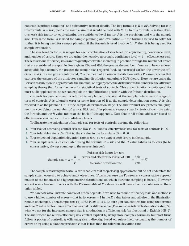
controls (attribute sampling) and substantive tests of details. The key formula is R = nP. Solving for n in this formula, n = R/P, yields the sample size that would be used with MUS. In this formula, R is the (effec-tiveness) risk factor or, equivalently, the confidence level factor; P is the precision; and n is the sample size. This same formula is used for sample planning and evaluation—if the formula is used to solve for n, then it is being used for sample planning; if the formula is used to solve for P, then it is being used for sample evaluation.

The risk level factor, R, is unique for each combination of risk level (or, equivalently, confidence level) and number of errors. Since we are using the negative approach, confidence level = 1 − effectiveness risk. The less-serious efficiency risks are frequently controlled indirectly in practice through the number of errors that are considered acceptable. For a given RIA and MM, the greater the number of errors to be considered acceptable by a sample, the greater the sample size required (and, as discussed earlier, the lower the effi-ciency risk). In case you are interested, R is the mean of a Poisson distribution with a Poisson process that captures the essence of the attributes sampling distribution underlying MUS theory. Here we are using the Poisson distribution to approximate the binomial or hypergeometric distributions that underlie the attribute sampling theory that forms the basis for statistical tests of controls. This approximation is quite good for most audit applications, so we can exploit the simplifications possible with the Poisson distribution.

P stands for precision and is referred to as planned precision at the sample determination stage. In tests of controls, P is tolerable error or some fraction of it at the sample determination stage. P is also referred to as the planned UEL at the sample determination stage. The auditor must use professional judg-ment in specifying the number of errors, RIA, and P in planning sample sizes for tests of controls using the formula and the R value tables at the back of this appendix. Note that the R value tables are based on effectiveness risk values = 1 − confidence levels.

To illustrate the calculation of sample size for tests of controls, assume the following:

1. Your risk of assessing control risk too low is 1%. That is, effectiveness risk for tests of controls is 1%. 2. Your tolerable rate is 6%. That is, the P value in the formula is 6% = 0.06. 3. Your expected population deviation rate is zero, so we expect zero errors in the sample. 4. Your sample size is 77 calculated using the formula R = nP and the R value tables as follows (to be

conservative, always round up to the nearest integer):

Sample size = n = R

P =

Poisson risk factor for zero errors and effectiveness risk of 0.01

tolerable deviation rate =

4.61

0.06 = 77

The sample sizes using the formula are reliable in that they closely approximate but do not understate the sample sizes necessary to achieve audit objectives. (This is because the Poisson is a conservative approxi-mation of the binomial and hypergeometric distributions on which attribute sampling is based.) However, since it is much easier to work with the Poisson table of R values, we will base all our calculations on the R value tables.

We can now also illustrate control of efficiency risk. If we wish to reduce efficiency risk, one method is to use a higher number of errors—that is, let errors = 1 in the R value tables and all else in the illustration remain unchanged. Then sample size (n) = 6.64/0.06 = 111. Be sure you can confirm this using the formula and the R value tables. Since effectiveness risk is still the same (1%) and so is tolerable deviation rate (6%), what we get for the increased sample size is a reduction in efficiency risk (as illustrated in Exhibit 10B–2). The auditor can make this efficiency risk control explicit by using more-complex formulas, but most firms follow a policy of controlling efficiency risk indirectly, based on subjectively estimating the number of errors or by using a planned precision P that is less than the tolerable deviation rate.

Fourth Pass


smi87468_app10B_10B1-10B67 10B-14 09/15/15 07:17 PM

The effect of using a lower planned precision in sample determination can also be illustrated. Let us assume the auditor uses a planned precision of 3% rather than the tolerable error rate of 6%. Now we get a sample size n = 4.61/0.03 = 154. Again, effectiveness risk is 1% and tolerable error rate is still 6% (it will be used in the sample evaluation decision rule for deciding if the sample error rate is acceptable), so that what the auditor obtains with the increased sample size is, again, a reduction in efficiency risk. A common way to reduce the planned precision from what is material or tolerable is to subtract the expected error rate from the material or tolerable error rate. For example, if the toler-able rate is 0.06 and the expected error rate is 0.03, then planned precision is 0.06 − 0.03 = 0.03. This is the main reason for considering the expected error rate in the audit under MUS. The expected error rate reduces the planned precision, thereby increasing the sample size and reducing the efficiency risks. This is true for either tests of controls or substantive tests of balances. Since sample size can be increased to virtually any amount, most audit firms put a restriction on planned precision by not let-ting it get below one half the tolerable deviation rate.

More about Defining Populations: StratificationAuditors can be flexible when defining populations. Accounting populations are often skewed, meaning that much of the dollar value in a population is in a small number of population units. For example, the 80/20 rule is that 80% of the value tends to be in 20% of the units. Many inventory and accounts receiv-able populations have this skewness. Sales invoice, cash receipt, and cash payment populations may be skewed, but usually not as much as inventory and receivables balances.

Theoretically, a company’s control procedures should apply to small-dollar as well as to large-dollar transactions. Nevertheless, many auditors believe that evidential matter is better when more dollars are covered in the test of controls part of the audit. This inclination can be accommodated in a sampling plan by subdividing (stratifying) a population according to a relevant characteristic of interest. For example, sales transactions might be subdivided into foreign and domestic, accounts receivable might be subdivided into sets of customers with balances of $5,000 or more and those with smaller balances, and payroll trans-actions might be subdivided into supervisory (salaried) and hourly payroll.

Nothing is wrong with this kind of stratification. However, you must remember that (1) an audit con-clusion based on a sample applies only to the population from which the sample was drawn and (2) the sample should be representative—random for statistical sampling. If 10,000 invoices represent 2,000 for-eign sales and 8,000 domestic sales, and you want to subdivide the population this way, you will have two

Review Checkpoints10B-9 What facts, estimates, and judgments do you need to figure a test of controls sample size using

the R value tables? What other relevant judgment is not used?

10B-10 Test yourself to see whether you can get the sample size of 87 from the R value table with these

specifications: effectiveness risk = 5%, tolerable deviation rate = 9%, expected errors = 3.

10B-11 What facts, estimates, and judgments do you need to figure a test of controls sample size using

the R value tables and Poisson risk factors? What other relevant judgment is not used?

10B-12 Test yourself to see whether you can get the sample size of 70 using the Poisson risk factor equation

with these specifications: effectiveness risk = 5%, tolerable deviation rate = 9%, expected errors = 2.

Fourth Pass


smi87468_app10B_10B1-10B67 10B-15 09/15/15 07:17 PM

populations. You can establish decision criteria of acceptable risk of assessing control risk too low and tolerable deviation rate for each population. You can also estimate an expected population deviation rate for each one. Suppose your specifications are these:

FOREIGN DOMESTIC

Risk of assessing control risk too low 5% 10%

Tolerable deviation rate 5 5

Expected population deviation rate 2 1

Then, sample size (R value tables; assume P is adjusted for expected error rate, e.g., foreign P = 0.05 – 0.02 = 0.03) is

100 58

You can evaluate each sample separately using the appropriate risk of assessing control risk too low, or you can combine the sample. To combine the sample sizes effectively, you would have to make the most conservative assumptions among the strata objectives. In the illustration, this means using an overall com-bined risk of assessing control risk too low of 10% and an expected combined population (strata) deviation rate of 1% so that both efficiency and effectiveness risks are at the lower of the two sample sizes.

Interestingly, if the population had not been stratified but treated as one population of 10,000 invoices, and the criteria had been effectiveness risk = 10%, tolerable deviation rate = 5%, and expected error rate = 1%, the sample size would be 58. Subdividing in two a population subject to test of controls sampling has the practical effect of doubling the extent of sampling. This is the price we pay for being able to make sepa-rate statistical statements about each stratum—the audit issue becomes: how important is it to evaluate the strata separately?

A Little More about Sampling-Unit Selection MethodsAudit sampling can be wrecked on the shoals of auditors’ impatience. Planning an imaginative selection method takes a little time, and auditors are sometimes in a big hurry to grab some units and audit them. A little imagination goes a long way. For example, suppose an auditor of a newspaper publishing client needs to audit the controls over the completeness of billings—specifically, the control procedure designed to ensure that customers were billed for classified ads printed in the paper. You have probably seen classified ad sections, so you likely know they consist of different-size ads, and you know that ad volume is greater on weekends than on weekdays. How can you get a random sample that can be considered representative of the printed ads?

The physical frame of printed ads defines the population. You probably cannot obtain a population count (size) of the number of ads. However, you know that the paper was printed on 365 days of the year, and the ad manager can probably show you a record of the number of pages of classified ads printed each day. Using this information, you can determine the number of ad pages for the year, say, 5,000. For a sample of 100 ads, you can choose 100 random numbers between 1 and 5,000 to obtain a random page. Then, you can choose a random number between 1 and 10 to identify one of the 10 columns on the page, and another random number between 1 and 500 (the number of lines on a page). The column-line coordi-nate identifies any ad on the random day. (This method approximates randomness, because larger ads are more likely to be chosen than smaller ads. In fact, the selection method probably approximates a sample selection stratified by the size of the ads.)

You can judge the representativeness by noticing the size of the ads selected. Also, since you will know the number of Friday-Saturday-Sunday pages (say, 70% of the total, or 3,500 pages), you can expect about 70 of the ads to come from weekend days.

Fourth Pass


smi87468_app10B_10B1-10B67 10B-16 09/15/15 07:17 PM

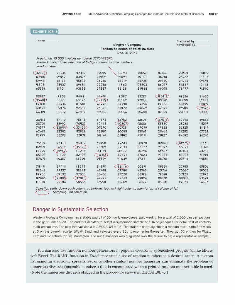
Random Number TableThe most accurate, although also most time-consuming, sampling unit selection device is a table of random digits, as in the one at the back of this appendix. This table contains rows and columns of digits from 0 to 9 in random order. When items in the population are associated with numbers in the table, the choice of a random number amounts to the choice of a sampling unit, and the resulting sample is ran-dom. Such a sample is called an unrestricted random sample. For example, in a population of 10,000 sales invoices, assume the first invoice in the year was 32071 and the last one was 42070. By obtaining a random start in the table and proceeding systematically through it, 100 invoices may be selected for audit.2 Assume that a random start is obtained at the five-digit number in the second row, 50th column—number 29094—and that the reading path in the table is down to the bottom of the column, then to the top of the next column, and so on. The first usable number and first invoice is 40807, the second is 32146, and so forth. Note that several of the random numbers were skipped because they did not correspond to the invoice number sequence.3 A page of random digits like the one at the back of this appendix can be annotated and made into your sample selection working paper to document the selection, as shown in Exhibit 10B–6.

Systematic Random SelectionAnother selection method commonly used in auditing because of its simplicity and relative ease of application is systematic random selection. This method is employed when direct association of the population with random numbers is cumbersome. Systematic selection consists of (a) dividing the population size by the sample size, obtaining a quotient k (a “skip interval”); (b) obtaining a random start in the population file; and (c) selecting every kth unit for the sample. A file of credit records is a good example. These may be filed alphabetically with no numbering system. Therefore, to select 50 from a population of 5,000, first find k = 5,000/50 = 100, then obtain a random start in the first 100 of the set of physical files, and pull out every 100th one thereafter, progressing systematically to the end of the file and returning to the beginning of the file to complete the selection. This method only approximates randomness, but the approximation can be improved by taking more than one random start in the process of selection. When more than one start is used, the interval k is changed. For example, if five starts are used, then every 500th item is selected. Five random starts give you five systematic passes through the population, and each pass produces 10 sampling items, for a total of 50.

Auditors usually require five or more random starts. You can see that when the number of random starts equals the predetermined sample size, the “systematic” method becomes the same as the unrestricted random selection method. Multiple random starts are a good idea because a population may have a non-random order that could be embedded in a single-start systematic method.

Computerized SelectionMost audit organizations have computerized random number generators available to cut short the drudg-ery of poring over printed random number tables. Such routines can print a tailored series of numbers with relatively brief turnaround time. Even so, some planning is required, and knowledge of how a random number table works is useful.

unrestricted random sample:sample obtained by means of unrestricted random selection

Fourth Pass


smi87468_app10B_10B1-10B67 10B-17 09/15/15 07:17 PM

You can also use random number generators in popular electronic spreadsheet programs, like Micro-soft Excel. The RAND function in Excel generates a list of random numbers in a desired range. A custom list using an electronic spreadsheet or another random number generator can eliminate the problem of numerous discards (unusable numbers) that is encountered when a printed random number table is used. (Note the numerous discards skipped in the procedure shown in Exhibit 10B–6.)

Danger in Systematic SelectionWestern Products Company has a stable payroll of 50 hourly employees, paid weekly, for a total of 2,600 pay transactions in the year under audit. The auditors decided to select a systematic sample of 104 paycheques for detail test of controls audit procedures. The skip interval was k = 2,600/104 = 25. The auditors carefully chose a random start in the first week at 3 on the payroll register (Wyatt Earp) and selected every 25th payroll entry thereafter. They got 52 entries for Wyatt Earp and 52 entries for Bat Masterson. The audit manager was disgusted over the failure to get a representative sample!

9541699859681552543751904

1925800301009361 507605212

8741056992338445234206293

76 1 311 6 91 93496991 10990357

5774179337595924188022346

3294207410599 814625165558

99187356411 40316067766314

2041628701745796261593945

7568902921142950530357071

7847189242149554244618534

4233983828456736965493123

864211609681 5189255467859

7564670423334268296822879

96837354241 42168240312901

1359959293970353741554556

5904521409762109971627887

1 6 40134775484402604289356

641766241507570755400 8 161

674509320903 1 914031208899

8439047481804304747217558

2669329094582191 1 56353138

1 939721562022182347220056

8275240807007288004501442

44 51 15 213361 6476 2 19 19 1 039

3214 607740872200451373689

4905765 1 1445738088032 1488

8329797983047566986930648

6360698086070795306975071

5042487327302966702367251

0087143345063924949414894

8749636701295508602709095

4 01 1 145040195066287787349

370 1 158850193222066521427

8284895897666679007328701

0935425716790280886005030

2062425762247365186778777

4932619200606951958420389

5734628968563252128294842

419756 517110 10 18320503846

227457002057123080381 956 1

1 4819128270957412 1 1 671240

8168616383884943957653805

6951245297848190776826210

7166320376632037134494589

6580654005528724362456517

Population: 10,000 invoices numbered 32701–42070.Method: unrestricted selection of 5-digit random invoice numbers.Random Start:

Index Prepared byReviewed by

Selection path: down each column to bottom, top next right column, then to top of column at left Sampling unit selection.

Kingston CompanyRandom Selection of Sales Invoices

Dec. 31, 20X2

EXHIBIT 10B–6

Fourth Pass


smi87468_app10B_10B1-10B67 10B-18 09/15/15 07:17 PM

Statistical EvaluationTo accomplish a statistical evaluation of test of controls audit evidence, you must know the tolerable rate and the acceptable effectiveness risk. These are your decision criteria—the standards for evaluation under the circumstances. You also need to know the size of the sample that was audited and the number of devia-tions. Now you can use the R value tables to make the evaluation. Again you use the Poisson risk factors in the R value tables, except now you use the R = nP formula to solve for P to get achieved precision = com-puted upper error limit = UEL: P = R/n. You already know n since you have already selected the sample; R is obtained from the R value tables with your knowledge of the number of errors found and planned effectiveness risk.

For example, suppose you audited a sample of 90 sales transactions and found 2 of them without proper shipping documents. Previously, you had decided an effectiveness risk of 5% was appropriate.

Using the formula above, UEL = Poisson risk factor for number of errors = effectiveness risk divided by sample size.

For example, the Poisson risk factor for effectiveness risk = 5% and 2 errors (deviations) found in a sample is 6.30; thus, with a sample of 90, UEL = 6.30/90 = 0.07, or 7%.

Applying a Decision RuleAfter you calculate the UEL, you can compare it to your previously determined tolerable deviation rate and apply an appropriate decision rule. Note that you do not compare the computed UEL to the planned precision that you used in determining the sample size if the planned precision was less than the tolerable rate. As discussed earlier, the sole reason for using a planned precision less than tolerable is to control for efficiency risk through a larger sample size. In sample evaluation, the planned precision has no role to play because we use the achieved precision resulting from the actual sample results.

A higher control risk assessment decision is not the same as a “rejection” decision. You can take the UEL derived from your sample and use it to assess the control risk. For example, assume you audited 30 sales transactions (tolerable deviation rate criterion of 8%, an effectiveness risk criterion of 10%, and an expecta-tion of zero deviations) to try to evaluate control risk at 0.40 (see Exhibit 10B–3) and justify the audit of 107 customer accounts in the accounts receivable total (see Exhibit 10B–4). You can achieve this control risk assessment if you find no deviations in the sample of 30 transactions (see the R value tables). If you find one actual deviation in the sample of 30, your computed UEL is 14% (see the R value tables and use the formula), and according to the decision rule, you should not assess control risk at 0.40. However, you can take UEL = 14%, assess a higher control risk (0.70 according to Exhibit 10B–3), and audit a sample of 130 customer accounts, which is appropriate for control risk of 0.70, instead of the sample of 107 appropriate if control risk had been assessed at 0.40.

Review Checkpoints10B-13 When you subdivide a population into two populations for attribute sampling, how do the two

samples compare to the one sample that would have been drawn if the population had not been

subdivided?

10B-14 Are you required to use all five digits of a random number when you have a random number table,

such as the one at the end of this appendix?

10B-15 What steps are involved in selecting a sample using the systematic random selection method?

Fourth Pass


smi87468_app10B_10B1-10B67 10B-19 09/15/15 07:17 PM

The computed upper error limit is a statistical calculation that takes sampling error into account. You know that a sample deviation rate (number of actual deviations in the sample divided by sample size) can-not be expressed as the exact population deviation rate. According to common sense and statistical theory, the actual but unknown population rate might be lower or higher. Since auditors are mainly concerned with the risk of assessing control risk too low (because it relates to the more-serious effectiveness risk), the higher limit is calculated to show how high the estimated population deviation rate may be.

Auditing standards tell you to “consider the risk that your sample deviation rate can be lower than your tolerable deviation rate for the population, even though the actual population rate exceeds the tol-erable rate.” In statistical evaluation, you accomplish this consideration by holding the risk of assessing the control risk too low constant at the acceptable level while computing UEL and then comparing UEL to your tolerable deviation rate. In short, if achieved UEL > tolerable error for tests of controls, then reject reliance at planned level; otherwise, you can rely. How much reliance depends on the auditor’s judgment and the decision rule he or she uses. (Exhibit 10B–3 is an example of such a decision rule.)

Example of Satisfactory ResultsSuppose you selected 200 recorded sales invoices and vouched them to supporting shipping orders. You found no shipping orders for one invoice. When you followed up, no one could explain the missing documents, but nothing about the sampling unit appeared to indicate an intentional irregularity. You have already decided that a 10% risk of assessing control risk too low—that is, effectiveness risk for test of controls = 10%—and a 3% tolerable deviation rate, adequately define your decision criteria for the test of controls audit. Calcu-late UEL using the R = nP formula and the R value tables. From R = nP solve for P: P = R/n. From the R value tables find the appropriate value for R using effectiveness risk = 10% and 1 error: R = 3.89. So the calculated upper error limit = UEL = 3.89/200 = 1.945%.

Audit conclusion: The probability is 10% that the population deviation rate is greater than 2%. This finding (UEL of 2%, less than tolerable rate of 3%) satisfies your decision criteria, and you can assess control risk as you had originally planned.

Example of Unsatisfactory ResultsThe situation is the same as above, except you found four invoices with missing shipping orders. Now, P = R/n = 8/200 = 4% = computed upper error limit = UEL.

Audit conclusion: The probability is 10% that the population deviation rate is greater than 4%. This UEL finding exceeds your tolerable rate criterion of 3%, and you ought to assess a higher control risk than you had originally planned.

Test of Controls Decision RuleIf the computed UEL is less than your tolerable deviation rate, you can conclude that the population deviation rate is low enough to meet your tolerable rate decision criterion, and you can assess the control risk at the level associated with the tolerable deviation rate. (Alternatively, you can assess the control risk at the level associated with the UEL, or you can calculate a probability associated with the tolerable deviation rate based on the sample data.)

If UEL exceeds your tolerable deviation rate, you can conclude that the population deviation rate may be higher than your decision criterion, and you should assess a higher control risk—for example, the control risk associated with the UEL.

Fourth Pass


smi87468_app10B_10B1-10B67 10B-20 09/15/15 07:17 PM

Discovery Sampling—Fishing for FraudDiscovery sampling is essentially another kind of sampling design directed toward a specific objective. However, discovery sampling statistics also offer an additional means of evaluating the sufficiency of audit evidence in the event that no deviations are found in a sample.

A discovery sampling table is obtainable from the R value tables by simply reading the entries for the zero-errors line. That is, no errors are considered acceptable in the sample. As indicated in Exhibit 10B–1, this results in the highest efficiency risk over the range of immaterial errors. A discovery sampling plan deals with the following kind of question: If I believe some important kind of error or irregularity might exist in the records, what sample size will I have to audit to have assurance of finding at least one example? Ordinar-ily, discovery sampling is used to design procedures to search for such things as examples of forged cheques or intercompany sales improperly classified as sales to outside parties. However, discovery sampling may be used effectively whenever a low deviation rate is expected. Auditors must quantify a desired probability of at least one occurrence when the specified tolerable deviation rate occurs. In discovery sampling the tol-erable deviation rate is frequently referred to as the critical rate of occurrence. Generally, the critical rate is very low because the deviation is something very sensitive and important, such as a sign of fraud.

The probability in this case represents the desired probability of finding at least one occurrence (exam-ple of the deviation) in a sample. In the R value tables, you can read across the zero-errors column for the desired effectiveness risk (the effectiveness risk in the zero-errors row represents the probability of at least one occurrence), and critical rate is simply the P value in our formula: R = nP.

To illustrate, suppose that in the test of controls audit of recorded sales, you are especially concerned about finding an example of a deviation of as few as 50 outright fictitious sales (intentional irregularities) existing in the population of 10,000 recorded invoices (a critical rate of 0.5%). Furthermore, suppose you want to achieve at least 0.99 probability (or, in percentage terms, 99% probability) of finding at least one. The R value tables and our formula indicate a required sample size of 922 recorded sales invoices, as fol-lows: n = R/P = 4.61/0.005 = 922. If a sample of this size were audited and no fictitious sales were found, you could conclude that the actual rate of fictitious sales in the population was less than 0.5% with 0.99 probability of being right.

This feature of discovery sampling evaluation provides the additional means of evaluating the suf-ficiency of audit evidence whenever an attribute sample turns up zero deviations. You can scan across the different effectiveness risk tables at the back of this appendix until you find an R value in the zero-errors row that comes just below the one associated with the lowest effectiveness risk. As an illustration, suppose 200 sales invoices were audited and no deviations of missing shipping orders were found. The R value tables show that if the population deviation rate is 2%, the probability of including at least 1 deviation in a sample of 200 is 0.98 (i.e., R = nP = 200 × 0.02 = 4—the highest R value in the zero-errors rows of the R value tables not exceeding 4 occurs with effectiveness risk = 0.02—the complement of this risk is the prob-ability of finding more than zero errors). None were found, so, with 0.98 probability, you can believe that the occurrence rate of missing shipping orders is 2% or less.

Review Checkpoints10B-16 What is the auditing interpretation of the sampling error–adjusted deviation rate (UEL)?

10B-17 What is the UEL for these data: sample size audited = 46, actual deviations found = 3, effectiveness

risk = 35%?

10B-18 What is the proper interpretation of the probability in discovery sampling?

Fourth Pass


smi87468_app10B_10B1-10B67 10B-21 09/15/15 07:17 PM

Putting It All TogetherTo this point, you have learned some of the theoretical details about defining populations, perceiving con-trol risk as a probability ranging from low (e.g., 0.10) to high (e.g., 1.0), using smoke/fire multiple thinking to determine an anchor tolerable deviation rate, and using tables and Poisson risk factor calculations to determine the test of controls sample size (n). You also learned about an assignment of successively higher tolerable deviation rates to successively higher control risks as a means of identifying each control risk level with a tolerable deviation rate.

You also learned about the links that connect tests of controls sampling for control risk assessment to substantive sampling for the audit of an account balance. These links are (1) the smoke/fire multiplier judgment that relates tolerable dollar misstatement in the substantive balance-audit sample to the anchor tolerable deviation rate in the test of controls sample and (2) methods that relate an audit judgment of risk of incorrect acceptance for the substantive balance-audit sample to the risk of incorrect acceptance consequences of assessing control risk too low. There is one more link: (3) considering the cost of the substantive balance-audit sample to decide the test of controls sample size and the planned control risk assessment. The planned control risk assessment, with the emphasis on planned, is the auditors’ selection of a control risk level for which they want to justify a control risk assessment after completing the test of controls audit work. Conceptually, the auditor should pick that strategy of control testing combined with substantive tests of detail that minimizes total audit cost. This can be done formally through use of explicit cost assumptions or informally, for example, as in Exhibit 10B–3. Most firms use the informal approach, probably to facilitate implementation and a certain consistency and audit quality across all clients, and because cost estimates may not be that accurate.

Summary of Sampling for Tests of ControlsStatistical sampling for attributes in test of controls auditing provides quantitative measures of deviation rates and risks of assessing control risk too low. The statistics support the auditors’ professional judg-ments involved in control risk assessment. The most important judgments are the numbers assigned to the tolerable rate of deviation, the risk of assessing control risk too low, and the risk of assessing control risk too high. With these specifications and an estimate of the deviation rate in the population, a preliminary sample size can be determined. However, nothing is magic about a predetermined sample size. It will turn out to be too few, just right, or too many, depending on the evidence produced by it and the control risk assessment supported by it.

The easy part of attribute sampling is the statistical evaluation. The hard parts are (1) specifying the controls for audit and defining deviations, (2) quantifying the decision criteria, (3) using imagination to find a way to select a random sample, and (4) associating the quantitative evaluation with the assessment of control risk. The structure and formality of the steps involved in statistical sampling force auditors to plan the procedures exhaustively. The same structure and formality also contribute to good working paper

Review Checkpoints10B-19 What are the links that connect test of controls sample planning with substantive balance-audit sample

planning?

10B-20 When you have several alternative test of controls sample sizes to choose from, how do you choose

the one to audit?

Fourth Pass


smi87468_app10B_10B1-10B67 10B-22 09/15/15 07:17 PM

documentation because they clearly identify the things that should be recorded in the working papers. Alto-gether, statistical sampling facilitates auditors’ plans, procedures, and evaluations of defensible evidence.

Part III: Audit of an Account BalanceMost of the account balances that appear in financial statements consist of numerous subsidiary accounts, some more numerous than others. Many of these accounts may be audited with sampling methods—auditing less than 100% of the subsidiary accounts within a control account balance or financial statement total for the purpose of determining the fair presentation of one or more of the financial statement assertions. Some examples of such accounts are listed here:

• Cash: Usually not audited by sampling because there are few accounts; might be sampled if a company has a large number of bank accounts

• Accounts receivable: Usually audited by sampling when there is a modest to large number of customers • Inventory: Usually audited by sampling when there is a modest to large number of different inventory

items • Fixed assets: Sampling sometimes used to audit numerous additions or an “inventory-taking” of fixed

assets • Accounts payable: Some sampling used, but normally a judgment sample for missing payables • Notes payable: Usually not audited by sampling because of small number

This short list and description of accounts, however, is not a description of relevant data populations for all assertions. For example, you would select a sample from the recorded accounts receivable to audit for the existence, rights, valuation, and presentation and disclosure assertions, but not for the complete-ness assertion. To audit for missing accounts receivable, the recorded ones are the wrong population! (A selection of shipping documents to determine whether receivables from customers had been recorded, or an audit of cash receipts in the period after year-end to detect receipts applicable to the prior year, could be proper samples for auditing for accounts receivable completeness.) Likewise, a selection of recorded accounts payable does not produce evidence of completeness of liabilities recordings. After all, the unrecorded liabilities are not in that population. (A selection of cash payments made after the year-end to identify ones applicable to year-end liabilities could be one proper sample for auditing for liability completeness.)

The audit of an account balance with monetary-value sampling has a different objective than test of controls auditing with attribute sampling. Test of controls sampling has the main objective of produc-ing evidence about the rate of deviation from company control procedures for the purpose of assessing the control risk. Measuring the monetary effect of control deviations is a secondary consideration. On the other hand, a test of an account balance has the objective of producing direct evidence of monetary amounts of error in the account. This is called monetary-value sampling to indicate that the important unit of measure is a monetary amount (such as dollars, pennies, renminbi, euros, or yen). Sometimes, monetary-value sampling is called variables sampling just to distinguish it from attributes sampling and the control risk assessment objective.

There are two main types of monetary-value sampling. The one most frequently used in financial audit-ing is MUS. This method is the subject covered here. The other method is known as classical sampling—a name attached merely to distinguish it from MUS. Classical sampling is discussed briefly at the end of this appendix. The method is called “classical” because it was used before MUS was developed and because it

Fourth Pass


smi87468_app10B_10B1-10B67 10B-23 09/15/15 07:17 PM

depends on the well-known statistical mathematics of the normal distribution. MUS, by contrast, does not depend upon the normal distribution statistics.

Before we get to the techniques of MUS, however, two topics of common application need to be expanded—the risk of incorrect acceptance and the risk of incorrect rejection.

Risk of Incorrect AcceptanceIn Chapter 10, you saw the audit risk model expanded to include these terms:

AR = IR × CR × APR × RIA

Monetary-value sampling for account balance auditing is primarily concerned with the risk of incor-rect acceptance (RIA) in the risk model. The risk of incorrect acceptance is also called the test of details risk because it is the sampling risk of failing to detect a materiality magnitude of monetary error with audit procedures applied to the details (subsidiary units) in a control account. The other elements of the model are products of auditors’ professional judgment.

The audit risk (AR) is the overall risk the auditor is willing to take of failing to discover material misstatement in the account. Public accounting firms that quantify this risk usually set it at 0.05 or 0.10. Their policies are somewhat arbitrary, because there is no overall theory acceptable in the practice world to justify any particular quantification of the audit risk. The amounts of 5% and 10% just seem to work adequately.

The inherent risk (IR) is the auditors’ assessment of general factors relating to the probability of erro-neous transactions entering the accounting system in the first place. It is hard to assess, often consisting of auditors’ memory of no problems in previous audits or other aspects of their knowledge of the business. Some public accounting firms have questionnaires to document the findings of the know-the-business pro-cedures and to translate them into an inherent risk assessment.

Analytical procedures were introduced in Chapter 8. They basically consist of all evidence-gathering procedures other than direct audit of account details. They are substantive procedures, as are the substan-tive tests of details, but they are not applied on a sample basis. Thus, there is frequently no mathematical way to measure their risk of failure. The analytical procedures risk (APR) in the model is the auditors’ judgment of the probability that these non-detail procedures will fail to detect misstatement in the amount of tolerable misstatement in the account. Public accounting firms that quantify this risk assign values from 0.30 to 1.0.

The control risk (CR) is the auditors’ assessment of the quality of the client’s control structure. Control risk assessment was explained in detail in Chapters 9 and 10. Some public accounting firms combine the inherent risk judgment and the control risk assessment into one factor.

These risk elements are considered independent, meaning that their combined risk can be a product (multiplication). While theoretical arguments of the validity of the model rage, several public accounting firms have built it into their sampling plans. They determine the risk of incorrect acceptance for a sampling application by first making AR, IR, CR, and APR judgments and assessments, and then calculating the risk of incorrect acceptance:

Maximum RIA = 0.50, if the equation produces RIA > 0.50

However, be forewarned—not all public accounting firms or other audit organizations use the model in this fashion. Some quantify risk of incorrect acceptance for statistical sampling in the context of the client situation without reference to the model. Some say they do sampling without quantifying risk of incorrect acceptance. Some say they do audit sampling, but not statistical sampling. Practice varies.

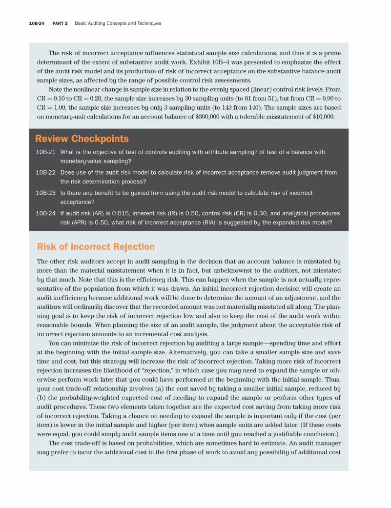
Fourth Pass


smi87468_app10B_10B1-10B67 10B-24 09/15/15 07:17 PM

The risk of incorrect acceptance influences statistical sample size calculations, and thus it is a prime determinant of the extent of substantive audit work. Exhibit 10B–4 was presented to emphasize the effect of the audit risk model and its production of risk of incorrect acceptance on the substantive balance-audit sample sizes, as affected by the range of possible control risk assessments.

Note the nonlinear change in sample size in relation to the evenly spaced (linear) control risk levels. From CR = 0.10 to CR = 0.20, the sample size increases by 30 sampling units (to 81 from 51), but from CR = 0.90 to CR = 1.00, the sample size increases by only 3 sampling units (to 143 from 140). The sample sizes are based on monetary-unit calculations for an account balance of $300,000 with a tolerable misstatement of $10,000.

Risk of Incorrect RejectionThe other risk auditors accept in audit sampling is the decision that an account balance is misstated by more than the material misstatement when it is in fact, but unbeknownst to the auditors, not misstated by that much. Note that this is the efficiency risk. This can happen when the sample is not actually repre-sentative of the population from which it was drawn. An initial incorrect rejection decision will create an audit inefficiency because additional work will be done to determine the amount of an adjustment, and the auditors will ordinarily discover that the recorded amount was not materially misstated all along. The plan-ning goal is to keep the risk of incorrect rejection low and also to keep the cost of the audit work within reasonable bounds. When planning the size of an audit sample, the judgment about the acceptable risk of incorrect rejection amounts to an incremental cost analysis.

You can minimize the risk of incorrect rejection by auditing a large sample—spending time and effort at the beginning with the initial sample size. Alternatively, you can take a smaller sample size and save time and cost, but this strategy will increase the risk of incorrect rejection. Taking more risk of incorrect rejection increases the likelihood of “rejection,” in which case you may need to expand the sample or oth-erwise perform work later that you could have performed at the beginning with the initial sample. Thus, your cost trade-off relationship involves (a) the cost saved by taking a smaller initial sample, reduced by (b) the probability-weighted expected cost of needing to expand the sample or perform other types of audit procedures. These two elements taken together are the expected cost saving from taking more risk of incorrect rejection. Taking a chance on needing to expand the sample is important only if the cost (per item) is lower in the initial sample and higher (per item) when sample units are added later. (If these costs were equal, you could simply audit sample items one at a time until you reached a justifiable conclusion.)

The cost trade-off is based on probabilities, which are sometimes hard to estimate. An audit manager may prefer to incur the additional cost in the first phase of work to avoid any possibility of additional cost

Review Checkpoints10B-21 What is the objective of test of controls auditing with attribute sampling? of test of a balance with

monetary-value sampling?

10B-22 Does use of the audit risk model to calculate risk of incorrect acceptance remove audit judgment from

the risk determination process?

10B-23 Is there any benefit to be gained from using the audit risk model to calculate risk of incorrect

acceptance?

10B-24 If audit risk (AR) is 0.015, inherent risk (IR) is 0.50, control risk (CR) is 0.30, and analytical procedures

risk (APR) is 0.50, what risk of incorrect acceptance (RIA) is suggested by the expanded risk model?

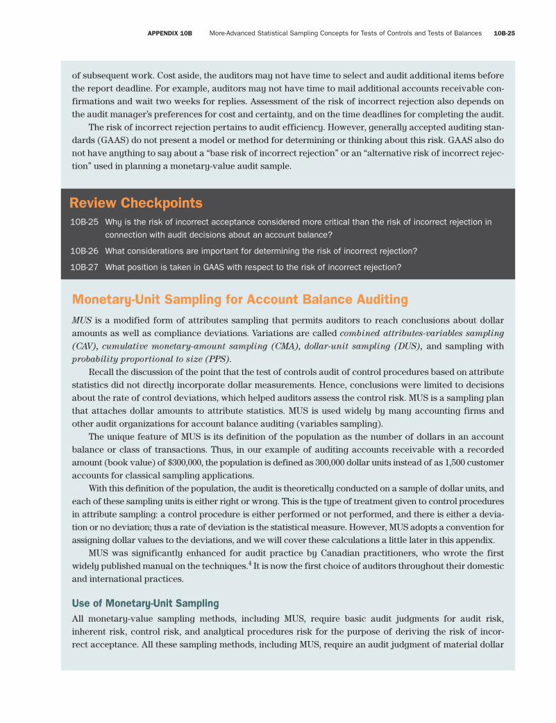
Fourth Pass


smi87468_app10B_10B1-10B67 10B-25 09/15/15 07:17 PM

of subsequent work. Cost aside, the auditors may not have time to select and audit additional items before the report deadline. For example, auditors may not have time to mail additional accounts receivable con-firmations and wait two weeks for replies. Assessment of the risk of incorrect rejection also depends on the audit manager’s preferences for cost and certainty, and on the time deadlines for completing the audit.

The risk of incorrect rejection pertains to audit efficiency. However, generally accepted auditing stan-dards (GAAS) do not present a model or method for determining or thinking about this risk. GAAS also do not have anything to say about a “base risk of incorrect rejection” or an “alternative risk of incorrect rejec-tion” used in planning a monetary-value audit sample.

Monetary-Unit Sampling for Account Balance AuditingMUS is a modified form of attributes sampling that permits auditors to reach conclusions about dollar amounts as well as compliance deviations. Variations are called combined attributes-variables sampling (CAV), cumulative monetary-amount sampling (CMA), dollar-unit sampling (DUS), and sampling with probability proportional to size (PPS).

Recall the discussion of the point that the test of controls audit of control procedures based on attribute statistics did not directly incorporate dollar measurements. Hence, conclusions were limited to decisions about the rate of control deviations, which helped auditors assess the control risk. MUS is a sampling plan that attaches dollar amounts to attribute statistics. MUS is used widely by many accounting firms and other audit organizations for account balance auditing (variables sampling).

The unique feature of MUS is its definition of the population as the number of dollars in an account balance or class of transactions. Thus, in our example of auditing accounts receivable with a recorded amount (book value) of $300,000, the population is defined as 300,000 dollar units instead of as 1,500 customer accounts for classical sampling applications.

With this definition of the population, the audit is theoretically conducted on a sample of dollar units, and each of these sampling units is either right or wrong. This is the type of treatment given to control procedures in attribute sampling: a control procedure is either performed or not performed, and there is either a devia-tion or no deviation; thus a rate of deviation is the statistical measure. However, MUS adopts a convention for assigning dollar values to the deviations, and we will cover these calculations a little later in this appendix.

MUS was significantly enhanced for audit practice by Canadian practitioners, who wrote the first widely published manual on the techniques.4 It is now the first choice of auditors throughout their domestic and international practices.

Use of Monetary-Unit SamplingAll monetary-value sampling methods, including MUS, require basic audit judgments for audit risk, inherent risk, control risk, and analytical procedures risk for the purpose of deriving the risk of incor-rect acceptance. All these sampling methods, including MUS, require an audit judgment of material dollar

Review Checkpoints10B-25 Why is the risk of incorrect acceptance considered more critical than the risk of incorrect rejection in

connection with audit decisions about an account balance?

10B-26 What considerations are important for determining the risk of incorrect rejection?

10B-27 What position is taken in GAAS with respect to the risk of incorrect rejection?

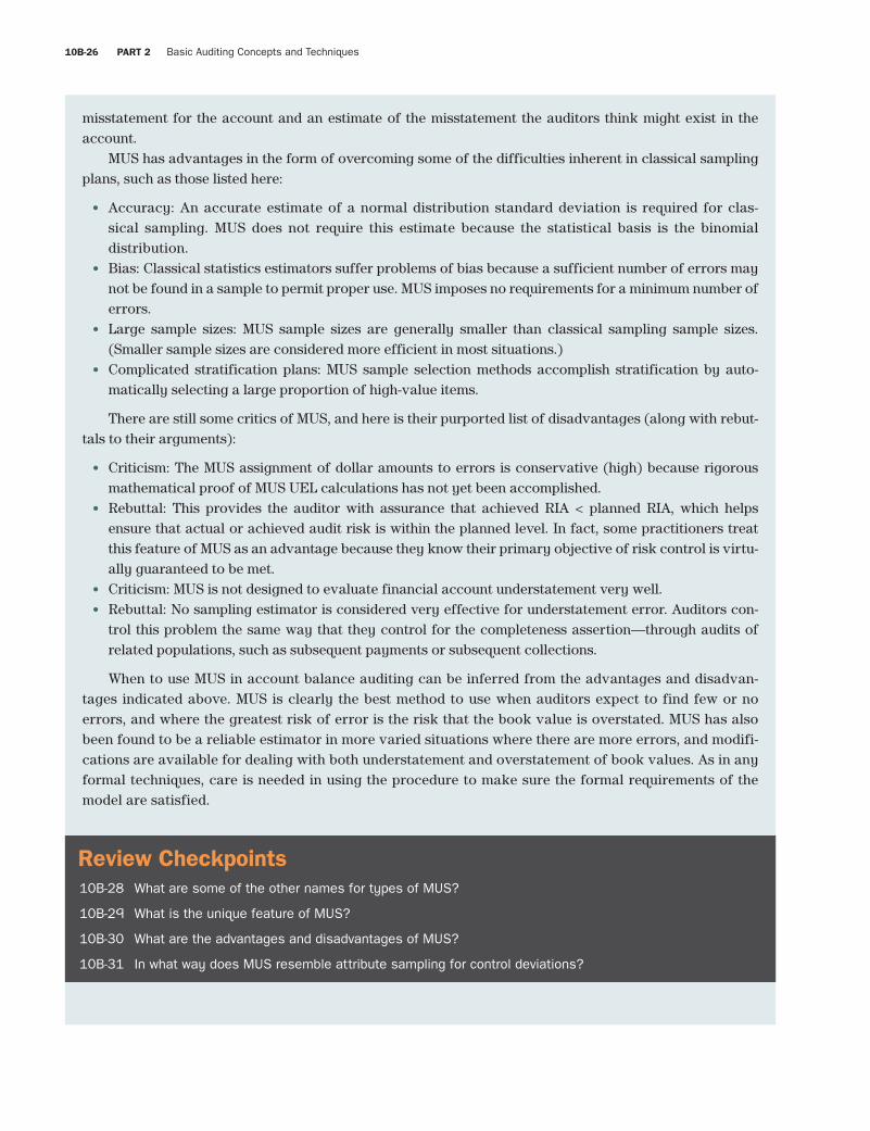
Fourth Pass


smi87468_app10B_10B1-10B67 10B-26 09/15/15 07:17 PM

misstatement for the account and an estimate of the misstatement the auditors think might exist in the account.

MUS has advantages in the form of overcoming some of the difficulties inherent in classical sampling plans, such as those listed here:

• Accuracy: An accurate estimate of a normal distribution standard deviation is required for clas-sical sampling. MUS does not require this estimate because the statistical basis is the binomial distribution.

• Bias: Classical statistics estimators suffer problems of bias because a sufficient number of errors may not be found in a sample to permit proper use. MUS imposes no requirements for a minimum number of errors.

• Large sample sizes: MUS sample sizes are generally smaller than classical sampling sample sizes. (Smaller sample sizes are considered more efficient in most situations.)

• Complicated stratification plans: MUS sample selection methods accomplish stratification by auto-matically selecting a large proportion of high-value items.

There are still some critics of MUS, and here is their purported list of disadvantages (along with rebut-tals to their arguments):

• Criticism: The MUS assignment of dollar amounts to errors is conservative (high) because rigorous mathematical proof of MUS UEL calculations has not yet been accomplished.

• Rebuttal: This provides the auditor with assurance that achieved RIA < planned RIA, which helps ensure that actual or achieved audit risk is within the planned level. In fact, some practitioners treat this feature of MUS as an advantage because they know their primary objective of risk control is virtu-ally guaranteed to be met.

• Criticism: MUS is not designed to evaluate financial account understatement very well. • Rebuttal: No sampling estimator is considered very effective for understatement error. Auditors con-

trol this problem the same way that they control for the completeness assertion—through audits of related populations, such as subsequent payments or subsequent collections.

When to use MUS in account balance auditing can be inferred from the advantages and disadvan-tages indicated above. MUS is clearly the best method to use when auditors expect to find few or no errors, and where the greatest risk of error is the risk that the book value is overstated. MUS has also been found to be a reliable estimator in more varied situations where there are more errors, and modifi-cations are available for dealing with both understatement and overstatement of book values. As in any formal techniques, care is needed in using the procedure to make sure the formal requirements of the model are satisfied.

Review Checkpoints10B-28 What are some of the other names for types of MUS?

10B-29 What is the unique feature of MUS?

10B-30 What are the advantages and disadvantages of MUS?

10B-31 In what way does MUS resemble attribute sampling for control deviations?

Fourth Pass


smi87468_app10B_10B1-10B67 10B-27 09/15/15 07:17 PM

Monetary-Unit Sample Size CalculationThe same formula is used for substantive testing of details as for testing of controls: n = R/P. The only adjustment is that planned precision must be converted from a dollar amount to a rate or percentage, as is used in control testing. This is achieved by simply dividing the planned precision in dollars by the recorded amount of the account balance.

The basic equation for calculating an MUS sample size for substantive testing of details is

n = (BV × R)/MM

where

BV = Total book value (recorded amount) of the account balance

R = Poisson risk factor appropriate for the risk of incorrect acceptance (RIA or effectiveness risk)

MM = Material misstatement for the account balanceNote that the above formula follows from n = R/P if we let P = MM/BV. That is, planned precision P is

represented as a rate in testing of details by dividing material misstatement by the reported amount of the account balance.

The recorded amount (BV) is the book balance of the account under audit, for example, a $300,000 accounts receivable total for 1,500 customers, subject to auditing by sampling.

The concept of material misstatement was covered in Chapter 8.As in attributes sampling, efficiency risk (risk of incorrect rejection) is usually controlled indirectly

following either or both of the following approaches: (a) select a number of errors greater than zero, and/or (b) use a planned precision that has been reduced by the amount of expected misstatement. For example, in using approach (b) assume that expected misstatement is EM; then planned precision to be used in the denominator in sample determination is (MM/BV − EM/BV) = (MM − EM)/BV. Auditors who use this technique do not allow planned precision to get below one half of MM/BV. Note that firms using this rule and setting the number of errors at zero in the R value tables never plan higher than twice the discovery sample for the given risk of incorrect acceptance (RIA = 1 − confidence level). To illustrate, assume, as before in Chapter 10, that MM = $10,000. Then a discovery sample size (the smallest possible for RIA = 1%) is n = 4.61/(10,000/300,000) = 4.61/0.0333 = 139 (round up to be con-servative). If the auditor wishes to accept a sample with one error and all else remains unchanged, the sample size will be n = 6.64/0.0333 = 200. Note that since risk of incorrect acceptance and materiality are the same, what the auditor gets for this increased work is a reduction in risk of incorrect rejection. (Remember Exhibit 10B–1.)

The other way to reduce risk of incorrect rejection is by adjusting planned precision P for expected misstatements (EM). As an illustration, assume EM = 4,000; then sample size can be increased to n = 4.61/((10,000 − 4,000)/300,000) = 4.61/(0.0333 − 0.0133) = 4.61/0.02 = 231.

Note that in the numerator we use the R value with zero errors, since we are already controlling risk of incorrect acceptance through the tighter precision (0.02 versus 0.0333) in the denominator. There is, thus, little need to combine the adjustment of planned precision approach with the zero-errors approach in con-trolling risk of incorrect rejection with MUS.

More formal, explicit approaches are available for controlling risk of incorrect rejection and risk of incorrect acceptance simultaneously, but since the basic principles are the same, we do not cover these refinements here.

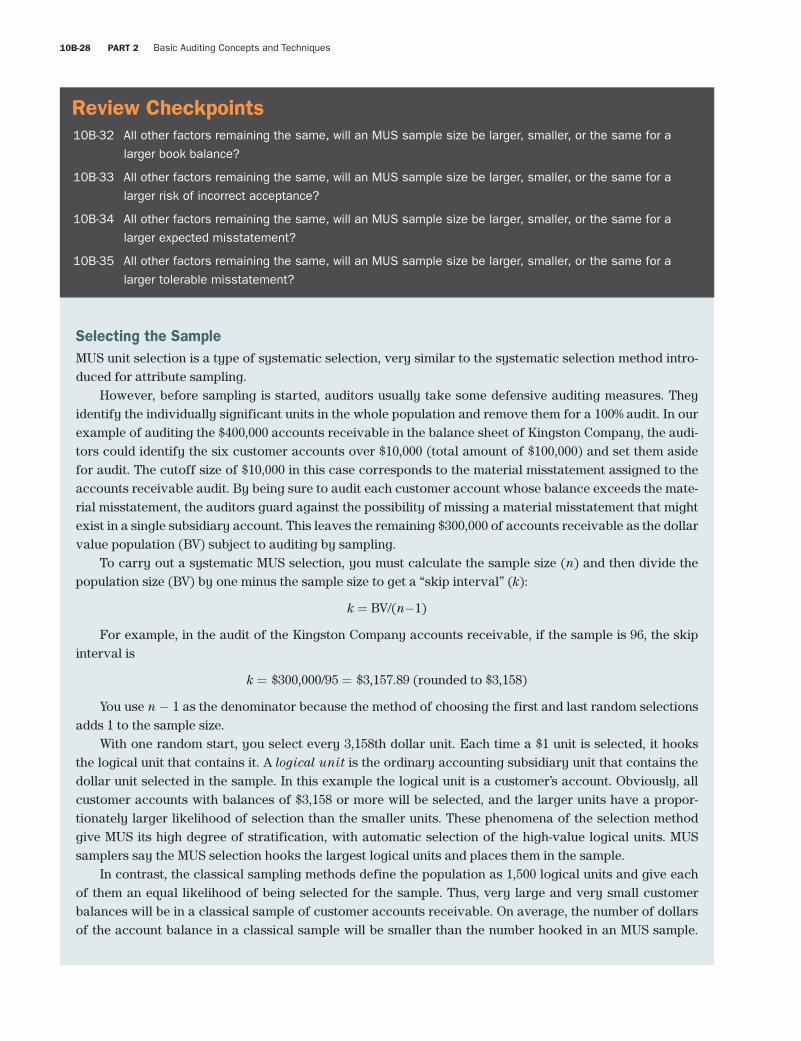
Fourth Pass


smi87468_app10B_10B1-10B67 10B-28 09/15/15 07:17 PM

Selecting the SampleMUS unit selection is a type of systematic selection, very similar to the systematic selection method intro-duced for attribute sampling.

However, before sampling is started, auditors usually take some defensive auditing measures. They identify the individually significant units in the whole population and remove them for a 100% audit. In our example of auditing the $400,000 accounts receivable in the balance sheet of Kingston Company, the audi-tors could identify the six customer accounts over $10,000 (total amount of $100,000) and set them aside for audit. The cutoff size of $10,000 in this case corresponds to the material misstatement assigned to the accounts receivable audit. By being sure to audit each customer account whose balance exceeds the mate-rial misstatement, the auditors guard against the possibility of missing a material misstatement that might exist in a single subsidiary account. This leaves the remaining $300,000 of accounts receivable as the dollar value population (BV) subject to auditing by sampling.

To carry out a systematic MUS selection, you must calculate the sample size (n) and then divide the population size (BV) by one minus the sample size to get a “skip interval” (k):

k = BV/(n-1)

For example, in the audit of the Kingston Company accounts receivable, if the sample is 96, the skip interval is

k = $300,000/95 = $3,157.89 (rounded to $3,158)

You use n − 1 as the denominator because the method of choosing the first and last random selections adds 1 to the sample size.

With one random start, you select every 3,158th dollar unit. Each time a $1 unit is selected, it hooks the logical unit that contains it. A logical unit is the ordinary accounting subsidiary unit that contains the dollar unit selected in the sample. In this example the logical unit is a customer’s account. Obviously, all customer accounts with balances of $3,158 or more will be selected, and the larger units have a propor-tionately larger likelihood of selection than the smaller units. These phenomena of the selection method give MUS its high degree of stratification, with automatic selection of the high-value logical units. MUS samplers say the MUS selection hooks the largest logical units and places them in the sample.

In contrast, the classical sampling methods define the population as 1,500 logical units and give each of them an equal likelihood of being selected for the sample. Thus, very large and very small customer balances will be in a classical sample of customer accounts receivable. On average, the number of dollars of the account balance in a classical sample will be smaller than the number hooked in an MUS sample.

Review Checkpoints10B-32 All other factors remaining the same, will an MUS sample size be larger, smaller, or the same for a

larger book balance?

10B-33 All other factors remaining the same, will an MUS sample size be larger, smaller, or the same for a

larger risk of incorrect acceptance?


larger expected misstatement?


larger tolerable misstatement?

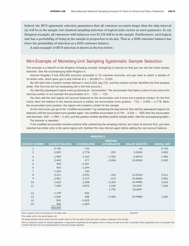
Fourth Pass


smi87468_app10B_10B1-10B67 10B-29 09/15/15 07:17 PM

Indeed, the MUS systematic selection guarantees that all customer accounts larger than the skip interval (k) will be in the sample, but classical sampling selection of logical units carries no such guarantee. In our Kingston example, all customers with balances over $3,158 will be in the sample. Furthermore, each logical unit has a probability of being in the sample in proportion to its size. That is, a $500 customer balance has twice the probability of selection as a $250 customer balance.

A mini-example of MUS selection is shown in the box below.

Mini-Example of Monetary-Unit Sampling Systematic Sample SelectionThis example is a takeoff on the Kingston Company example. Everything is reduced so that you can see the entire sample selection. See the accompanying table Kingston II.

Assume Kingston II has $30,000 accounts receivable in 15 customer accounts, and you want to select a sample of 10 dollar units, which gives you a skip interval of k = 30,000/9 = 3,333.

We still start with a random number between 1 and 3,333, say 722, and this random number identifies the first sampled dollar. (The first one will not necessarily fall in the first account.)

You identify subsequent logical units by starting an “accumulator.” The accumulator first takes a value of zero minus the starting number. In our example the accumulator is 0 − 722 = −722.

You then add the next logical unit account balances to the accumulator until it turns into a positive number. On the first round, when the balance in the second account is added, the accumulator turns positive: −722 + 3,500 = 2,778. When the accumulator turns positive, the logical unit contains a dollar for the sample.

On the next round, you go to the “modified accumulator” by subtracting the skip interval; then add the subsequent logical unit balances until the accumulator turns positive again. The modified accumulator is 2,778 − 3,333 = −555; then the accumulator next becomes –555 + 1,965 = 1,410, and this positive number identifies another sample dollar. (See the accompanying table.)

The process is repeated.If the modified accumulator remains positive after subtracting the sampling interval, as it does at account #12, you have

selected two dollar units in the same logical unit. Subtract the skip interval again before adding the next account balance.

KINGSTON II

ACCOUNT NUMBER ACCOUNT BALANCE ACCUMULATORMODIFIED

ACCUMULATOR DOLLAR SELECTED LOGICAL UNIT

1 $ 750 −722 1st $ 7502 3,500 2,778 −555 3,334th 3,500

3 1,965 1,410 −1,923 6,667th 1,9654 2,400 477 −2,856 10,000th 2,4005 949 −1,9076 563 −1,3447 1,224 −1208 3,211 3,091 −242 13,333rd 3,2119 2,961 2,719 −614 16,666th 2,961

10 1,622 1,008 −2,325 19,999th 1,62211 7,200 4,875 1,542 23,332* 7,200

−1,791 26,665*12 1,199 −59213 1,000 408 −2,925 29,998th 1,00014 500 −2,42515 956 −1,469

$30,000

Total of logical units in the sample of 10 dollar units .......................................................................................................... $24,609

*Two dollar units in the same logical unit.

The dollar-selected column starts with the random start at 722 and adds 3,333 each time a dollar is selected in the sample.

This is a selection routine for manual application. It may seem complicated at first glance, but it is really not hard to do with a calculator. When populations are on computer files, a routine like this one can be programmed to make the sample selection.

Fourth Pass


smi87468_app10B_10B1-10B67 10B-30 09/15/15 07:17 PM

Express the Error Evidence in DollarsThe problem with attribute sampling is how to express the results in terms of a deviation rate instead of in dollars. In an audit context, expressing results in dollars is more meaningful when the audit objective is a decision about the fair presentation of a balance expressed in dollars. Therefore, dollar-unit sampling adopts some conventions for expressing the error evidence in dollars.

The first step is to determine an average sampling interval. This amount is slightly different from the sample selection skip interval. The average sampling interval (ASI) is

ASI = BV

___ n

In our example of the audit of Kingston Company’s accounts receivable with a sample of 96 customer accounts,

ASI = $300,000/96 = $3,125

You can work with the average sampling interval instead of the skip interval if you remember that the first random dollar is selected from the first interval of dollar units (in this case, 3,125 dollar units) and then simply add 3,125 a total of n − 1 times (in this case 95 times) to select n − 1 additional dollar units.

Calculate an Upper Error Limit: The No-Error CaseThe UEL is a statistical estimate of the greatest amount of dollar error that might exist in an account balance, with a likelihood (risk of incorrect acceptance) that the actual amount of error might be even greater. The easiest UEL calculation arises when the sample is audited and no dollar misstatements are discovered. Then the calculation is5

UEL = ASI × R

In our example, suppose the auditors audited 96 of Kingston’s customers’ accounts and found nothing wrong, no misstatements or arguments. If the auditors wish to evaluate the “greatest amount of error that might exist” at a risk of incorrect acceptance of 0.17, they will find the Poisson risk factor for RIA = 0.17 and zero errors in the R value tables, which is 1.77, and calculate the UEL:

UEL = ASI × R= $3,125 × 1.77= $5,531

This calculation follows from our basic formula R = n × P, except now we solve for P instead of for n as we do at the sample size determination stage. That is, P = R/n = 1.77/96 = 0.0184375. This is the achieved UEL represented as a rate or percentage (keep in mind the attributes sampling theory basis for MUS). How do we

Review Checkpoints10B-36 What effect does the identification of individually significant logical units have on the size of the

recorded amount population for MUS?

10B-37 How does MUS sample selection produce an automatic stratification of choosing the high-value logical

units in a control account balance?

10B-38 What happens when two dollar units for the sample fall in the same logical unit?

Fourth Pass


smi87468_app10B_10B1-10B67 10B-31 09/15/15 07:17 PM

convert this to a dollar amount? Simple! Multiply by BV: 0.0184375 × $300,000 = $5,531. Remember, we divided by BV to convert precision to a percentage. So, now we must multiply by BV to convert UEL to a dollar amount.

The risk of incorrect acceptance represented by the choice of the Poisson risk factor should be the risk of incorrect acceptance derived from the risk model the auditor uses to plan the audit work. This risk of incorrect acceptance is one of the auditors’ decision criteria for accepting the book value as materially accurate or for rejecting it as appearing to contain a material misstatement. The calculated UEL is simi-lar to an attribute sampling computed UEL (that is why we represent both by UEL). The auditor can say, “Based on the quantitative evidence, I estimate the greatest amount of error in the population is UEL (rate of deviation for UEL), with a likelihood of risk of incorrect acceptance [effectiveness risk] that the amount of misstatement error [or in the case of attitude sampling, the rate of deviation] might be greater.” The risk of incorrect acceptance represents the risk associated with MUS. Of course, other sources of evidence may have been used to derive a particular risk of incorrect acceptance from audit risk (AR). The audit risk model reflects these other sources. So, although 1 – RIA reflects the assurance provided by MUS, the total assurance from control-reliance, analytical-review procedures as well as MUS is 1 – AR.

The UEL must have a reference point to mean something. The reference point is the material misstate-ment assigned to the account, and it is the other decision criterion. You can use it with a “UEL decision rule,” as expressed in the following box.

Using this UEL decision rule in our Kingston Company example, where the risk of incorrect accep-tance is 0.17 and the tolerable misstatement is $10,000, the decision is that the evidence shows the $300,000 accounts receivable does not appear to contain a material misstatement. The UEL of $5,531 at RIA = 0.17 is less than the material misstatement.

The phenomenon of measuring a UEL amount of misstatement when no errors were found in the sam-ple is a reflection of the partial knowledge given by a sample from the population instead of knowledge of the entire population. Similarly, in attribute sampling for detail test of controls, a UEL greater than zero is expressed even when no deviations are found in a sample. This kind of measurement of sampling error is frequently called “further misstatement remaining undetected in the balance.” Auditors can take it into account by calculating the UEL.

The zero-error UEL is actually a reflection of the sufficiency of audit evidence as represented by the size of the sample audited. If the sample size is very small, indicating limited knowledge of the population, the average sampling interval will be large, and the UEL will be high. In these circumstances, the failure of the UEL decision rule (i.e., UEL greater than MM) is an indication of not enough evidence (sample size too small).

Calculate an Upper Error Limit: When Errors Are FoundWhen a dollar-unit sample is audited, the auditors determine (1) the dollar amount of difference between the book value and the audit value of the logical unit—the account or invoice—that contains the sampled dollar, and (2) the ratio of this difference to the recorded amount of the logical unit. This ratio is called the tainting percentage or taint%:

Upper Error Limit Decision RuleUsing actual sample data, calculate the UEL of monetary misstatement. Compare this UEL to the material misstatement decision amount. If the UEL is larger, make the “rejection” decision. If the UEL is smaller, make the “acceptance” decision. Note that the decision is based on the amount considered material, MM, not the planned precision, which may be less than material in order to control risk of incorrect rejection.

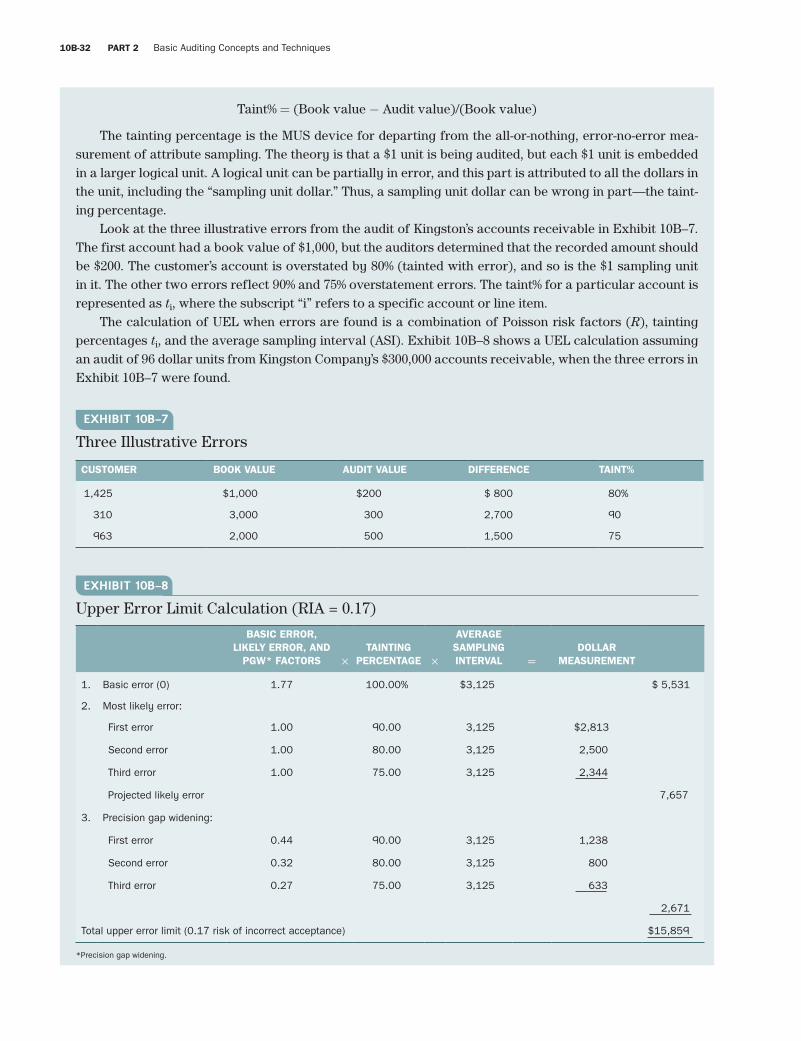
Fourth Pass


smi87468_app10B_10B1-10B67 10B-32 09/15/15 07:17 PM

Taint% = (Book value - Audit value)/(Book value)

The tainting percentage is the MUS device for departing from the all-or-nothing, error-no-error mea-surement of attribute sampling. The theory is that a $1 unit is being audited, but each $1 unit is embedded in a larger logical unit. A logical unit can be partially in error, and this part is attributed to all the dollars in the unit, including the “sampling unit dollar.” Thus, a sampling unit dollar can be wrong in part—the taint-ing percentage.

Look at the three illustrative errors from the audit of Kingston’s accounts receivable in Exhibit 10B–7. The first account had a book value of $1,000, but the auditors determined that the recorded amount should be $200. The customer’s account is overstated by 80% (tainted with error), and so is the $1 sampling unit in it. The other two errors reflect 90% and 75% overstatement errors. The taint% for a particular account is represented as ti, where the subscript “i” refers to a specific account or line item.

The calculation of UEL when errors are found is a combination of Poisson risk factors (R), tainting percentages ti, and the average sampling interval (ASI). Exhibit 10B–8 shows a UEL calculation assuming an audit of 96 dollar units from Kingston Company’s $300,000 accounts receivable, when the three errors in Exhibit 10B–7 were found.

CUSTOMER BOOK VALUE AUDIT VALUE DIFFERENCE TAINT%

1,425 $1,000 $200 $ 800 80%

310 3,000 300 2,700 90

963 2,000 500 1,500 75

EXHIBIT 10B–7

Three Illustrative Errors

*Precision gap widening.

BASIC ERROR, LIKELY ERROR, AND

PGW* FACTORS ×TAINTING

PERCENTAGE ×

AVERAGE SAMPLING INTERVAL =

DOLLAR MEASUREMENT

1. Basic error (0) 1.77 100.00% $3,125 $ 5,531

2. Most likely error:

First error 1.00 90.00 3,125 $2,813

Second error 1.00 80.00 3,125 2,500

Third error 1.00 75.00 3,125 2,344

Projected likely error 7,657

3. Precision gap widening:

First error 0.44 90.00 3,125 1,238

Second error 0.32 80.00 3,125 800

Third error 0.27 75.00 3,125 633

2,671

Total upper error limit (0.17 risk of incorrect acceptance) $15,859

EXHIBIT 10B–8

Upper Error Limit Calculation (RIA = 0.17)

Fourth Pass


smi87468_app10B_10B1-10B67 10B-33 09/15/15 07:17 PM

The “basic error,” calculated using the RF (risk factor) for the zero-error case, is the underlying sam-pling error associated with the sample size. It is weighted by a 100% tainting under the assumption that the maximum overstatement of a dollar unit is its recorded amount.

Next, the errors are put in descending order of their tainting percentages, the largest first and the smallest last. These are given a “likely error” factor of 1.0. The sum of 1.0 × respective tainting percent-ages × ASI for the errors is called the “projected likely error.” This is the auditor’s estimate of error based on the actual errors discovered ($5,000 = $800 + $2,700 + $1,500) projected to the population as $7,657.

The precision gap widening (PGW) is in addition to the sampling error generated by finding errors in the sample. These factors are in the R value tables. They bear a direct relationship to the Poisson risk (R) factors in the R value tables. Each PGW is the difference between the risk (R) factor for the error number and the risk (R) factor for the error number that preceded it minus 1.0 (the risk factor assigned to the actual error). Thus, the PGW for the first error at RIA = 0.17 is 0.44 = 3.21 − 1.77 − 1.00.

In terms of our UEL decision rule test of the accounts receivable, it appears that Kingston’s $300,000 accounts receivable may contain more than $10,000 material misstatement because the UEL of $15,859 is greater than $10,000 at risk of incorrect acceptance of 0.17. In other words, there is a 0.17 probability that overstatement in the receivables exceeds $15,859, when the auditors wanted to achieve a probability of 0.17 that misstatement could exceed only $10,000. We therefore have the “rejection” decision.

Exhibit 10B–8 calculations can be summarized by the following formula: (1/n) × (R0 + ((R1 − R0) × t1) + ((R2 − R1) × t2) + ((R3 − R2) × t3)) × BV = (1/n) × (R0 + ((1 + PGW1) × t1) + ((1 + PGW2) × t2) + ((1 + PGW3) × t3)) × BV = (1/n) × BV × (R0 + t1 + t2 + t3 + PGW1 × t1 + PGW2 × t2 + PGW3 × t3) = ((BV/n) × R) + ((BV/n) × (t1 + t2 + t3)) + ((BV/n) × ((PGW1 × t1) + (PGW2 × t2) + (PGW3 × t3))) = Basic error + Most likely error + Precision gap widening, where Basic error = ((BV/n) × R0), Most likely error = ((BV/n) × (t1 + t2 + t3)), and Precision gap widening = ((BV/n) × ((PGW1 × t1) + (PGW2 × t2) + (PGW3 × t3))). Note that (BV/n) is the sampling interval.

Although the above calculations may look rather complicated, they follow from the same evaluation formula used in testing of controls. Recall that achieved UEL in testing of controls for K errors found in the sample is P = R/n, where R is the Poisson risk factor for the specified effectiveness risk and K errors using the R value tables. This can be rewritten as follows:

R/n = (1/n) × (R0 + ∑Ki=1(Ri - Ri - l) × 1) = achieved UEL as a rate

In variables sampling, instead of just working with 0 and 1 values of attribute sampling (i.e., in the formula above there were K errors, or K “1” values, which determined the achieved UEL), one replaces the 1s with the concept of taintings. That is, instead of 1, use a tainting:

ti = (BVi - AVi)/BVi

It is through the concept of the tainting or fractional error that MUS is converted from a pure attributes sampling model to a variable sampling model that measures the total possible dollar error in a population.

The tainting concept has an interesting history. When MUS was first developed by Dutch statistician Dr. Van Heerden, he viewed it as a purely attributes sampling model applied to monetary units. There is no limit to how small the monetary unit can be, so the initial idea was to apply it to the smallest denomi-nation, say, the penny. In penny-unit sampling, you can apply strict attribute sampling because monetary error recorded is reducible only to the nearest penny. Thus, a penny is either in error or not. For exam-ple, suppose we have an accounts receivable recorded balance of 543.37, and we confirm that the actual amount is 347.85. Thus, under penny-unit sampling, 34,285 of the recorded pennies are “correct” while 54,337 − 34,785 = 19,552 of the pennies are completely in error; that is, there is a 19,552/54,337 = 36% recorded penny deviation rate in the account. From this perspective, we can view the entire accounts

Fourth Pass


smi87468_app10B_10B1-10B67 10B-34 09/15/15 07:17 PM

receivable population as having a certain attributes deviation rate, and attributes sampling is perfectly appropriate under such an interpretation. The only thing the auditor would have to do is develop a conven-tion to decide which penny of account A has been selected: one of the 19,552 pennies in error, or one of the 34,785 not in error. On selecting account A and determining the error, the auditor would have to use a con-sistent convention—for example, the in-error pennies can be assumed always at the head of the sequence of recorded pennies, such as the first 19,552 recorded pennies, not the last or the ones in the middle. Any consistent convention will do as long as the pennies in error continue having the same probability of being selected. Under such a convention there would be no need to modify any of the formulas used in testing of controls.

The difficulty with such an approach is that it may be impractical. For instance, if on following the con-vention the auditor knows of the $195.52 error but because of the convention he or she happens to select a penny not considered in error, the auditor would have to ignore this error. The auditor would be hard put to defend such an action in court!

The problem is that although such a convention is statistically valid, it is so in the long-term fre-quency sense, and the auditor has to consider the evidence in the specific case. So, as a compromise, auditors have developed the convention that when an account error is selected, the errors are presumed averaged in every monetary unit in the account. For this reason, the tainting is calculated and assumed to apply to every dollar unit, or penny unit, or whatever, in the misstated account. This approach maxi-mizes the information obtained from the sample. While this latter convention makes the treatment of errors in a given situation more acceptable to the auditor, and it closely approximates the “pure” conven-tion of Van Heerden, it does deviate from pure attribute sampling theory. Nevertheless, much research has shown this approach to result in conservative MUS bounds (the actual risk of incorrect acceptance is less than the planned level, or, to put it another way, the actual confidence level of MUS is greater than planned). This bias is acceptable and even considered preferable by many auditors because it means that the assurance they are getting from MUS is actually somewhat higher than what the formu-las indicate.

Calculate the Projected Likely MisstatementThe whole point of quantitative evidence evaluation is to extend the findings from the sample to the entire population. The first step is to calculate the projected likely misstatement, which is the auditors’ best esti-mate of misstatement based on the errors found in the sample. You can see the projected likely misstate-ment (PLM) of $7,657 at the middle right of Exhibit 10B–8.

Auditors are supposed to think about the amount of projected likely misstatement in relation to the material misstatement and consider whether there may be “further misstatement remaining undetected.” The difference between UEL and PLM ($8,202 = $15,859 − $7,657) is the MUS quasi-statistical measure-ment of sampling error and the “further misstatement remaining undetected.”

The projected likely misstatement plays a significant role in the auditors’ problem of deciding upon an amount to recommend for adjustment when they have made a “rejection” decision.

Determine the Amount of an AdjustmentThe problem of determining the amount to recommend for adjustment is troublesome because auditors usually do not know the exact amount of misstatement in an account. When the evidential base is a random sample, the three measurable aspects of monetary misstatement are (1) known misstatement, (2) projected likely misstatement, and (3) possible misstatement—the “further misstatement remaining undetected.”

Fourth Pass


smi87468_app10B_10B1-10B67 10B-35 09/15/15 07:17 PM

Quantitative ConsiderationsThe known misstatement is the sum of the actual dollar errors found in the sample. The projected likely misstatement is a calculation based on the known misstatements. Neither of these is affected by the auditors’ risk of incorrect acceptance criterion. However, the possible misstatement may be large or small. depending upon the risk of incorrect acceptance specification. This makes “possible misstatement” a slip-pery concept.

In our example of the audit of Kingston’s accounts receivable, we have

Known misstatement = $5,000PLM = $7,657

Possible misstatement = $8,202 (at RIA = 0.17)

The calculation of these components was illustrated earlier via the basic framework.Auditing standards and practice contain no hard and fast rules for determining the amount of adjust-

ment in sampling situations. Several measures of adjustment amounts can be derived from the data. Various sources have suggested the following:

• Adjust the amount of the known misstatement, in this case $5,000. Usually, the actual amount of known misstatement is smaller than the material misstatement. Often, this adjustment is too small and leaves too much potential for remaining error (in this case $10,859 = $15,859 − $5,000) unadjusted.

• Adjust the amount of the projected misstatement, in this case $7,657. The point estimate of likely mis-statement is considered the best single-value measurement available for recommending an adjustment to the client.

• In addition to adjusting for the projected likely misstatement amount, also adjust the amount of the possible misstatement, in this case another $8,202. This sum is the largest one an auditor can measure using the risk of incorrect acceptance in the audit plan. It contains an element of statis-tical measurement that auditors and clients may or may not be willing to accept for adjustment purposes.

• Adjust by the amount of material misstatement when the sum of projected and possible misstatement exceeds material misstatement, in this case $10,000. This kind of rule is somewhat arbitrary and is sub-ject to question when the sum exceeds 2 × MM.

• Adjust by the amount that the sum of projected and possible misstatement exceeds material misstate-ment, in this case $5,859 ($15,859 − $10,000). The theory here is that the amount of misstatement left in the account balance after adjustment will not exceed material misstatement ($10,000). This measure is somewhat arbitrary.

Statistical projections are used to recommend adjustment. Adjustments for known misstatements or projected misstatements have the most empirical and theoretical support. It can be shown that for any amount of error, sample size can be increased sufficiently so that adjusting for projected misstatements will always reduce the remaining error to less than a material amount at the stated confidence level. Of course, if the auditor cannot increase the sample size sufficiently, then the theo-retically best available adjustment is not an option and the auditor may have to rely on other audit procedures to determine the amount of adjustment or to make the appropriate reservation in the auditor’s report.

Not too much is known about public accounting firms’ use of statistical adjustments in financial audits, but, as noted in the following box, tax auditors may use such measures.

Fourth Pass


smi87468_app10B_10B1-10B67 10B-36 09/15/15 07:17 PM

As noted above, research suggests that adjusting for projected misstatement is a valid way of main-taining objective control of sampling risk after adjustment. For example, in Exhibit 10B–8 after adjust-ing accounts receivable for projected likely error of 7,657, a legitimate post-adjusted UEL with a risk of incorrect acceptance of 17% is 15,859 − 7,657 = 8,202—which would be an acceptable UEL under our deci-sion rule.

What happens if the difference between UEL and projected likely misstatement is greater than mate-rial? Then clearly an adjustment based on projected likely misstatement would not be sufficient. One way to develop an objective adjustment is to increase sample size. It can be shown that no matter how much error there is in the population, the difference between UEL and projected likely misstatement will be reduced as the sample size is increased. This means that theoretically there is a large enough sample size so that adjusting for projected likely misstatement will ensure that adjusted UEL is less than material and thus acceptable at the stated risk of incorrect acceptance level (or equivalently at a confidence level of 1 – RIA). Of course, as noted above, the auditor may not always be able to increase sample size as much as he or she needs.

Non-quantitative ConsiderationsYou can see that much latitude exists for determining the amount of an adjustment to recommend. Often, the amount recommended for one account depends on adjustment amounts recommended for other accounts. Auditors typically consider the findings in other audit areas when recommending adjustments.

The special characteristics of the accounts must also be considered. For example, in some cases the actual misstatement (overstatement in our Kingston accounts receivable example) may consist of over-charges to customers and undercharges from sales that were underbilled or simply not invoiced to cus-tomers (understatements). Management may make a policy decision not to try to recover the underbilled or unbilled amounts, so the audit manager must then deal with all the overstatement errors instead of a smaller net overstatement. Other accounts may be different. For example, both overstatements and under-statements in an inventory valuation may be adjustable simply by correcting the records, and no one needs to take customer relations into account.

Even though the lack of a definitive rule on how to figure the amount of an adjustment has revealed the lack of science in auditing, we can close the discussion with a more definite statement: as a general rule, all actual misstatements discovered in accounts audited completely should be adjusted, provided the amounts are material. The CPA Canada Handbook provides additional guidance, but first we must con-sider the case of both overstatement and understatement in the sample results.

Statistical Sampling as a Tool in Audits of Multinational ConcernsThe U.S. Internal Revenue Service (IRS) often tries to save resources in audits by projecting tax errors from samples of company data. It does this for travel and entertainment deductions. Now, the IRS is using sampling in challenging prices that a company charges for items sold to foreign subsidiaries. In such cases the IRS claims that a parent company is avoid-ing U.S. tax by undercharging its foreign units.

In a tax court dispute, Halliburton Company says the IRS was seeking to raise its income by $62.5 million for alleged underbilling; $29.5 million of the amount is from “adjustment for statistical sampling population.” The pending case shows that the IRS is using sampling more aggressively.

Source: Adapted from The Wall Street Journal, February 18, 1987.

Fourth Pass


smi87468_app10B_10B1-10B67 10B-37 09/15/15 07:17 PM

Overstatement and UnderstatementWhen both overstatement and understatement errors are discovered, you need to combine them properly. The calculations are not difficult.6 According to Leslie, Teitlebaum, and Anderson (1979):

1. Calculate separately the gross projected likely error (GPLEO) and the total upper error limit (TUELO) for overstatements, using an array of error taints only of the overstatement errors, ignoring under-statement errors.

2. Calculate separately the GPLEU and the TUELU for understatements, using an array of error taints only of the understatement errors, ignoring overstatement errors.

3. Calculate the net projected likely error (PLEN) by finding the net amount of the two gross projected likely error amounts, keeping track of whether the net amount is overstatement or understatement:

PLEN = GPLEO − GPLEU

4. Calculate the net upper limits (NUELO for overstatement and NUELU for understatement) by reducing each gross upper error limit (GUEL) by the gross projected likely error (GPLE) of the opposite direc-tion of misstatement; that is,

NUELO = TUELO − GPLEUNUELO = TUELU − GPLEO

The following example uses the overstatement amounts calculated in the preceding Kingston accounts receivable example and some hypothetical understatement amounts.

PROJECTED LIKELY ERROR

UPPER ERROR LIMIT

Gross errors:

Overstatements $7,657 $15,859

Understatements 5,000 10,000

Net errors:

Overstatements 2,657 10,859

Understatements NA = 0 2,343

NA means not applicable.

Now you can say that with risk of incorrect acceptance equal to the risk used to calculate both over-statement and understatement estimates, (1) the most likely misstatement amount is PLEN = $2,657

Review Checkpoints10B-39 Suppose you have audited a $600,000 recorded amount of inventory with a sample

of 100 dollar units and their logical units and found no errors. What is the UEL at

RIA = 0.05? RIA = 0.10? RIA = 0.25? RIA = 0.50?

10B-40 What is the risk-related interpretation of each of the UELs you calculated in question 10B-39?

10B-41 What is the UEL for the audit of 96 dollar units from the $300,000 accounts receivable, given the errors

shown in Exhibit 10B–7, for RIA = 0.48? for RIA = 0.05? What interpretation can you give to these UELs?

10B-42 If you had to pick the one best measure for an amount to recommend for adjustment based on a

sample, which one would you choose?

10B-43 Why do you think the auditing profession has no definite rules for deciding the amount of an adjustment?

Fourth Pass


smi87468_app10B_10B1-10B67 10B-38 09/15/15 07:17 PM

overstatement, but (2) the misstatement could be between NUELO = $10,859 overstatement and NUELU = $2,343 understatement. Since material misstatement for the receivables is $10,000, the total of $300,000 appears to be materially misstated because the NUELO exceeds $10,000.

With this background we can now develop operational guidelines for MUS adjustments consistent with the CPA Canada Handbook.

Audit Adjustments per the CPA Canada HandbookAccording to CAS 530.14, the auditor should estimate a likely aggregate misstatement by aggregating

(a) Known errors on other than representative samples

(b) Projection of misstatements on representative (e.g., statistical) samples (i.e., PLENs in MUS)

(c) Disagreements with accounting estimates

(d) Net effect of uncorrected misstatements in opening equity (note that this can include projections of misstatements

in some accounts, e.g., beginning inventory)

As noted in the earlier CICA Handbook, paragraph 5142.18–22, the above types of errors are aggregated in stages: in each stage the auditor determines whether the misstatement for each balance or class of transactions is material. If not, the auditor proceeds until the highest level of aggregation (net income, net assets) is reached.

If at any stage the auditor estimates a material likely aggregate misstatement, then the auditor should do the following:

(a) Arrange for the client to recheck the areas that contain the largest misstatements OR (b) Perform additional audit procedures (expand audit testing) OR (c) Insist on an adjustment OR (d) Issue a report reservation (CPA Canada Handbook, paragraph 5142.22)

An illustration of an adjustment based on known errors is given in Chapter 15. This example, however, does not consider projections or representative sample results.

The general rule in developing an adjustment policy for projections of errors based on statistical sam-pling is as follows (using the terminology in MUS mechanics):

1. If PLEN > materiality (situations 3 and 4 of AuG-41, paragraph 42), the auditor should insist on adjust-ment or, failing that, qualify the report. Note that PLEN is the same as = “Likely aggregate misstate-ment” (LAM) of the Risk and Materiality Guideline in the CICA Handbook.

2. If UEL net > materiality, but PLEN < materiality (situation 2 of AuG-41, paragraph 42, page 15), then the auditor will normally have to do further audit work to obtain more-persuasive evidence that mate-rial errors do not exist. Under this condition it is already improbable that (PLEN) material errors exist (since most likely errors projection lies below materiality) and so qualification may not be justified. But it is not sufficiently improbable without further work to justify a clear opinion (unless manage-ment agrees to some adjustments). Net UELs are also referred to as possible errors and in the risk and materiality guideline as further possible misstatements (less those due to non-sampling error). Since by definition non-sampling errors are impossible to measure objectively (e.g., the degree to which auditors inaccurately “take a random sample”), they are not explicitly considered in any formula.

The types of possible adjustments include the following:

1. Adjust for known errors only. Note that this can be applied to reduce both PLEN and UEL by the known errors. The auditor can then

use the above decision rules to decide if the population is acceptable after adjustment.

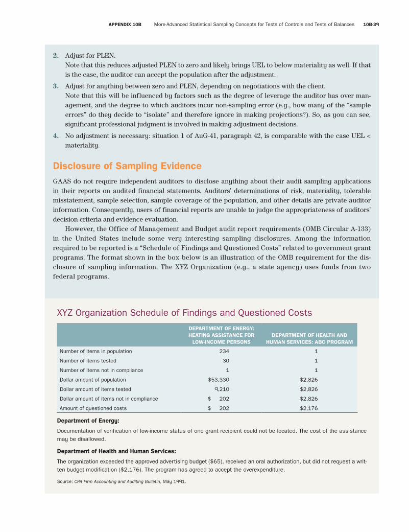
Fourth Pass


smi87468_app10B_10B1-10B67 10B-39 09/15/15 07:17 PM

2. Adjust for PLEN. Note that this reduces adjusted PLEN to zero and likely brings UEL to below materiality as well. If that

is the case, the auditor can accept the population after the adjustment.

3. Adjust for anything between zero and PLEN, depending on negotiations with the client. Note that this will be influenced by factors such as the degree of leverage the auditor has over man-

agement, and the degree to which auditors incur non-sampling error (e.g., how many of the “sample errors” do they decide to “isolate” and therefore ignore in making projections?). So, as you can see, significant professional judgment is involved in making adjustment decisions.

4. No adjustment is necessary: situation 1 of AuG-41, paragraph 42, is comparable with the case UEL < materiality.

Disclosure of Sampling EvidenceGAAS do not require independent auditors to disclose anything about their audit sampling applications in their reports on audited financial statements. Auditors’ determinations of risk, materiality, tolerable misstatement, sample selection, sample coverage of the population, and other details are private auditor information. Consequently, users of financial reports are unable to judge the appropriateness of auditors’ decision criteria and evidence evaluation.

However, the Office of Management and Budget audit report requirements (OMB Circular A-133) in the United States include some very interesting sampling disclosures. Among the information required to be reported is a “Schedule of Findings and Questioned Costs” related to government grant programs. The format shown in the box below is an illustration of the OMB requirement for the dis-closure of sampling information. The XYZ Organization (e.g., a state agency) uses funds from two federal programs.

XYZ Organization Schedule of Findings and Questioned Costs

DEPARTMENT OF ENERGY: HEATING ASSISTANCE FOR

LOW-INCOME PERSONSDEPARTMENT OF HEALTH AND

HUMAN SERVICES: ABC PROGRAM

Number of items in population 234 1

Number of items tested 30 1

Number of items not in compliance 1 1

Dollar amount of population $53,330 $2,826

Dollar amount of items tested 9,210 $2,826

Dollar amount of items not in compliance $ 202 $2,826

Amount of questioned costs $ 202 $2,176

Department of Energy:

Documentation of verification of low-income status of one grant recipient could not be located. The cost of the assistance may be disallowed.

Department of Health and Human Services:

The organization exceeded the approved advertising budget ($65), received an oral authorization, but did not request a writ-ten budget modification ($2,176). The program has agreed to accept the overexpenditure.

Source: CPA Firm Accounting and Auditing Bulletin, May 1991.

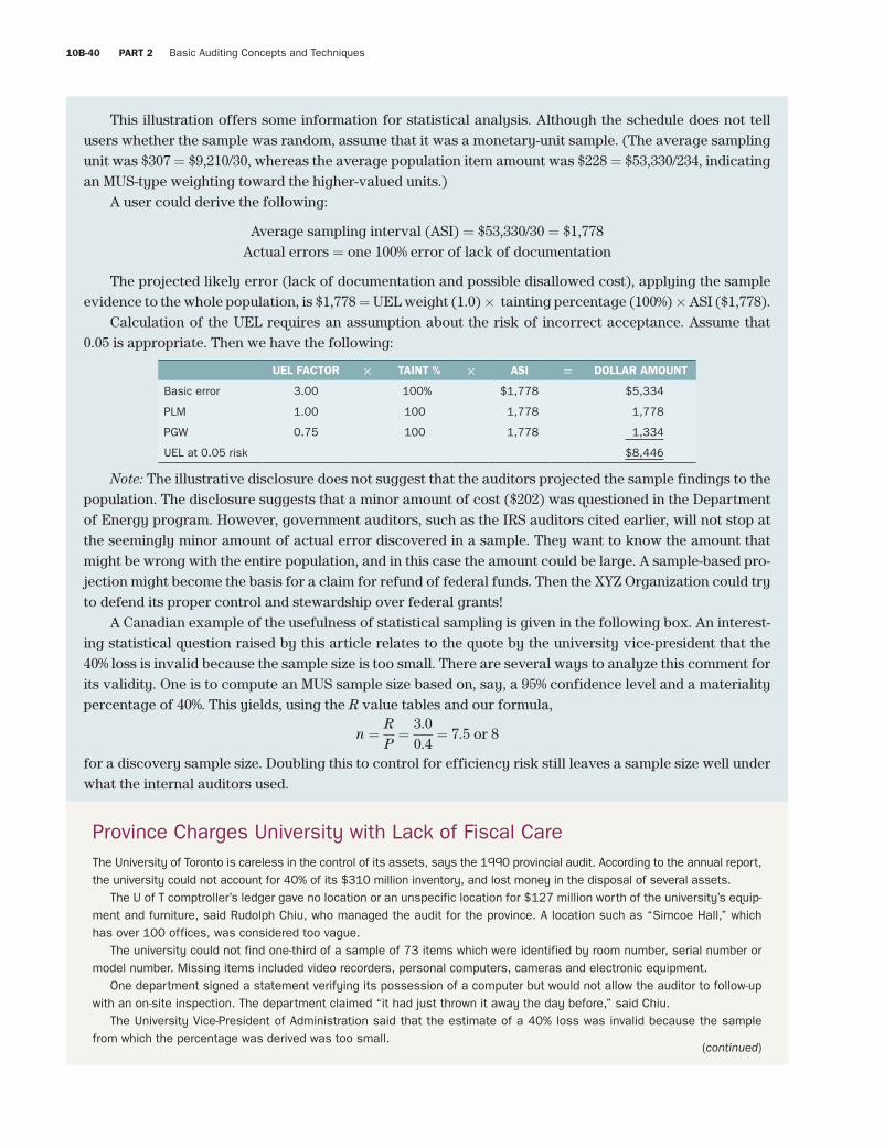
Fourth Pass


smi87468_app10B_10B1-10B67 10B-40 09/15/15 07:17 PM

This illustration offers some information for statistical analysis. Although the schedule does not tell users whether the sample was random, assume that it was a monetary-unit sample. (The average sampling unit was $307 = $9,210/30, whereas the average population item amount was $228 = $53,330/234, indicating an MUS-type weighting toward the higher-valued units.)

A user could derive the following:

Average sampling interval (ASI) = $53,330/30 = $1,778Actual errors = one 100% error of lack of documentation

The projected likely error (lack of documentation and possible disallowed cost), applying the sample evidence to the whole population, is $1,778 = UEL weight (1.0) × tainting percentage (100%) × ASI ($1,778).

Calculation of the UEL requires an assumption about the risk of incorrect acceptance. Assume that 0.05 is appropriate. Then we have the following:

UEL FACTOR × TAINT % × ASI = DOLLAR AMOUNT

Basic error 3.00 100% $1,778 $5,334

PLM 1.00 100 1,778 1,778

PGW 0.75 100 1,778 1,334

UEL at 0.05 risk $8,446

Note: The illustrative disclosure does not suggest that the auditors projected the sample findings to the population. The disclosure suggests that a minor amount of cost ($202) was questioned in the Department of Energy program. However, government auditors, such as the IRS auditors cited earlier, will not stop at the seemingly minor amount of actual error discovered in a sample. They want to know the amount that might be wrong with the entire population, and in this case the amount could be large. A sample-based pro-jection might become the basis for a claim for refund of federal funds. Then the XYZ Organization could try to defend its proper control and stewardship over federal grants!

A Canadian example of the usefulness of statistical sampling is given in the following box. An interest-ing statistical question raised by this article relates to the quote by the university vice-president that the 40% loss is invalid because the sample size is too small. There are several ways to analyze this comment for its validity. One is to compute an MUS sample size based on, say, a 95% confidence level and a materiality percentage of 40%. This yields, using the R value tables and our formula,

n = R

__ P

= 3.0

___ 0.4

= 7.5 or 8

for a discovery sample size. Doubling this to control for efficiency risk still leaves a sample size well under what the internal auditors used.

Province Charges University with Lack of Fiscal CareThe University of Toronto is careless in the control of its assets, says the 1990 provincial audit. According to the annual report, the university could not account for 40% of its $310 million inventory, and lost money in the disposal of several assets.

The U of T comptroller’s ledger gave no location or an unspecific location for $127 million worth of the university’s equip-ment and furniture, said Rudolph Chiu, who managed the audit for the province. A location such as “Simcoe Hall,” which has over 100 offices, was considered too vague.

The university could not find one-third of a sample of 73 items which were identified by room number, serial number or model number. Missing items included video recorders, personal computers, cameras and electronic equipment.

One department signed a statement verifying its possession of a computer but would not allow the auditor to follow-up with an on-site inspection. The department claimed “it had just thrown it away the day before,” said Chiu.

The University Vice-President of Administration said that the estimate of a 40% loss was invalid because the sample from which the percentage was derived was too small.

(continued)

Fourth Pass


smi87468_app10B_10B1-10B67 10B-41 09/15/15 07:17 PM

Another approach is to solve for the amount of error that would be considered material at sample size of 73 and a 95% confidence level (i.e., RIA = 0.05), and working backward solve 73 = 3.0/P. This yields a materiality of P = 3.0/73 = 0.041. In other words, the sample size was sufficient to detect an error rate of 4.1% or higher at a 95% confidence level. Several other analytical approaches could be followed, but they all point to the same consistent conclusion: the provincial auditor is likely correct and the 40% loss estimate is not invalid. Or, to put it in a more intuitive way, if you lost 40% of your belongings in a burglary you would realize it much more quickly than if, say, 1% of your belongings were missing. A vivid example of the importance of properly interpreting sample results and their consequences was provided by the uproar raised in February 2000 concerning federal spending on job grants. “The Boondoggle’s Big Picture” excerpt reproduces most of an article dealing with extrapolating the results of an internal audit and interpreting its social consequences.

“There’s no question we do not have an adequate way of checking inventory,” he added, “but it would cost us over a mil-lion dollars a year to hire someone to go out and physically check the equipment.” Budget reductions in 1979 forced the university to eliminate the three accounting positions responsible for checking inventory.

The report also criticized the university for failing to adhere to its own policy in the sale of equipment. The policy requires that the item be advertised and that a fair price be determined by the university purchasing department. If the sale is to an employee or relative of an employee, the sale must be approved by a university vice-president.

In one case, a six-month-old truck was sold unadvertised to a university employee at a 45% discount. One year later, the value of the truck was still higher than the sale price.

Criddle faulted an Ottawa truck dealer who had given the purchasing department too low a price on the truck. “The words [the auditor] chose give the wrong impression,” he said.

“It’s not a question of the university being careless,” he said, “It’s a question of people not following policy. That doesn’t surprise me. In a place this size there are a lot of procedures people don’t realize exist.”

He emphasized that the audit did not criticize the university for losing money, only for failing to adhere to its procedures.

Source: Adapted from Kate Zernike, The Newspaper, December 5, 1990. Used with permission from The Newspaper, University of Toronto’s Independent Community newspaper.

The Boondoggle’s Big PictureOttawa—Debate surrounding widespread financial mismanagement of government funds uncovered by an internal Human Resources audit has been dominated by 37 projects whose problems officials judged serious enough to require further review. Jean Chrétien, the Prime Minister, has rejected opposition suggestions of a “billion-dollar boondoggle” by stating, “It’s not $1-billion, it’s 37 cases. Some are worth $10,000 or less.”

However, extrapolating the problems identified by the audit sample across the total 30,000 projects from which the random sample was drawn shows thousands of projects could be in need of review.

The sample of 459 projects representing $200 million was drawn randomly from a total of 30,000 HRDC projects worth $1 billion a year in federal grants.

For a sample size of 459, Prof. Kalbfleisch said the true number of affected files can be estimated with an error of plus or minus 3%, 19 times out of 20.

The 35 affected files identified through the audit make up 7.6% of the sample. Extrapolated to 30,000 files, the esti-mated number of problem projects adds up to 2,280.

An error estimate of plus or minus 3% means the true number of affected grants would be between 4.6% and 10.6% of the total, or between 1,380 and 23,180 projects in all.

Prof. Kalbfleisch noted that the audit may not have been done by random sample, but by a stratified sample in which projects were chosen so as to represent geographic regions or grant sizes. In that case, the extrapolation would be more complex and the estimate of 2,280 would be incorrect. If the audit targets particularly high-risk files, for example, it could be an overestimate.

(continued)

Fourth Pass


smi87468_app10B_10B1-10B67 10B-42 09/15/15 07:17 PM

A number of other statistical issues are discussed at the end of this appendix following the questions. They include use of statistical regression in analytical review, use of MUS for compliance testing, and a more statistical interpretation of the audit risk model. It should be clear by now, however, that statistical auditing can help put auditing on a more scientific basis.

Ghislain Charron, a spokesman for HRDC, was not able yesterday to clarify the precise methodology of the audit.The internal audit looked at government-funded projects approved between April, 1997, and April, 1999. They ranged in

value from $300 to $14-million.Although only 37 projects were identified for further review, administrative problems were widespread. For example,

two-thirds of the projects did not contain an analysis or a rationale for recommending or accepting the project. Eight out of every ten reviewed projects did not show evidence of financial monitoring. Three out of four projects to which the govern-ment contributed money had no indication of monitoring for achievement of specific results.

Of 459 project files reviewed, 15% did not contain an application from the sponsor.

Source: Adapted from L. Chwialkowska, “Rot may have spread to 3,000 grants,” National Post, February 11, 2000, pp. A1 and A9.

A P P L I C AT I O N C A S E W I T H S O L U T I O N & A N A LY S I S

Monetary-Unit Sampling with Critical Thinking about Risk-Based Auditing

DISCUSSION CASE

The MUS concepts introduced in this chapter are good illustrations of the application of critical thinking, although the issues of critical thinking may be hidden in the assumptions underlying the mechanics of applying MUS. Can you identify the critical thinking steps, as outlined in Appendix 3A, in the MUS decision making as described in this appendix?

SOLUTION & ANALYSIS

Through MUS, the auditor arrives at a value for an accounting population. This is done by representative sampling (CAS 530).

Step 1 of critical thinking: Learn the views of others. In the sampling context, this step is represented by obtaining from management the total amount recorded for the population or some other claim about a population (e.g., that proper internal controls have been applied to the transactions of the reporting period).

The auditor’s views of the population for sampling purposes are relevant here. With MUS, the popula-tion is viewed as dollar units, with the total dollar amount recorded representing a population of individual dollars. The more traditional view, statistical sampling using tests based on the normal distribution, is of a population consisting of individual accounts or physical units of varying values (e.g., a population of individual accounts receivable or inventory items). These differences in viewpoints have consequences for the two theories themselves.

To summarize, effectiveness risk is the more serious as it relates directly to the audit risk model and its components, depending on whether we are talking about tests of controls or substantive tests.

Fourth Pass


smi87468_app10B_10B1-10B67 10B-43 09/15/15 07:17 PM

Effectiveness risk relates to audit effectiveness because the audit fails if it fails to detect a mate-rial misstatement. Efficiency risk, instead, relates to audit efficiency; it results in the auditors’ doing unnecessary work to clear up their mistake, something they are aware of by the end of the audit. This risk is implicitly controlled by the K value, as the higher the K value used in sample-size planning, the lower the efficiency risk and the larger the sample size. Another way to lower efficiency risk is to use a planned precision that is lower than overall or specific materiality. A common way to make this adjust-ment is to subtract expected errors from the overall or specific materiality. When auditors develop planned precision this way, they are really reducing efficiency risk over much of its range. (Remember that efficiency risk is controlled only at its lowest level; it grows automatically with the amount of mis-statement and reaches a peak at materiality.)

The differing theories result in planning differences, most notably in whether or not tolerable mis-statements or performance materialities of CAS 530.05 need to be less than overall materiality or specific materiality. These issues have also historically been related to whether materiality allocation is included in audit planning. Under MUS no allocation is needed. This means that MUS can restrict itself to using overall and specific materialities based on user needs in evaluating the sample results. In MUS, if the precision used in planning the sample size is a performance materiality, then the only reason for this is to help con-trol efficiency risk. The MUS formula examples below show this. For other statistical approaches, things are a bit more complicated. For these other statistical approaches, the model requirements, not user needs, make materiality allocation necessary.

MUS accommodates user needs by allowing the use of specific materialities of Chapter 5 without affecting the use of overall materialities in other populations. Also, the results of individual tests can be combined, as shown below, and the results compared with materiality for financial statements as a whole. In general, the process of combining the results of multiple tests is much simpler under MUS and helps explain its popularity.

Step 2: Identify the claims at issue. Management claims (asserts) that the recorded amount is materi-ally correct, and the main claim at issue is whether this is true or if, in fact, the population amount is mate-rially in error. The auditor must verify the assertion with the help of the statistical test.

Step 3: Reasons for the competing claims. Management will refer to its system of internal controls, corporate governance, and past track record. The auditor must be skeptical and consider the alternative claim that there is a material misstatement in the recorded amount, and show that the risk of this claim is at an appropriately low level (i.e., at an acceptable level).

Step 4: Evaluate the arguments. An argument, essentially, gives good reasons for a claim or conclu-sion. In statistical decision making, logically structured reasoning (see Appendix 3A, available on Con-nect, for more details) follows a pattern that is consistent with decision making throughout auditing and accounting.

The pattern of logical argumentation is as follows. First, identify assumptions (including theories), models, concepts, and principles that guide the overall reasoning process. MUS’s distinctiveness is in view-ing the population of interest as a population of dollar units and then applying attribute sampling theory to the dollar-unit population. With theories, many assumptions need to be made; some are more controversial than others, and critical thinking focuses on the more controversial ones, aiming to demonstrate their rea-sonableness. Often, the issues are a matter of firm policy, and much of the justification is embedded in firm practice manuals and policies.

Second, gather the evidence in conformity with the theory and consistent with the goal of the audit procedure. This includes proper specification of the population to be evaluated, as discussed in the chap-ter. For example, in representative sampling, each unit of the population must have a predictable chance of

Fourth Pass


smi87468_app10B_10B1-10B67 10B-44 09/15/15 07:17 PM

being selected. This is absolutely essential for objectively controlling sampling risk, which is the primary advantage of statistical audit techniques.

Third, reach a conclusion about the population that is consistent with the theory. For MUS, the conclu-sion is reached using the following decision rule:

Decision Rule (1):If achieved P > materiality or tolerable deviation rate, then reject the recorded amount for the popula-

tion; otherwise, accept it.This simple decision rule is effectively an evaluation of management’s claim that there is no material

error in the population or that no intolerable deviation rates exist in it.Step 5: Reach a conclusion. The decision rule above indicates the quantitative result. The auditor

must also consider qualitative aspects of the sample information, such as nature and cause of errors, before coming to a decision (CAS 530 and AuG-41). The above decision rule has already incorporated key quantitative risk and materiality considerations in the decision-making process.

Further Elaboration of the Critical Thinking Aspects of Adopting Monetary-Unit Sampling

Once a formal theory, such as MUS, has been accepted to assist in auditor decision making, it can be used to illustrate some basic concepts of auditing. For example, using our formulas and R value tables we can illustrate the law of diminishing marginal assurance to testing that explains why auditors use the sampling (testing) concept. For example, assuming materiality has a value of 0.01 (1%), then the sample sizes (n = R/P) for confidence levels of 80%, 95%, and 99%, respectively (equivalent effectiveness risks of 20%, 5%, and 1%), are as follows: 161, 300, and 451. Confidence levels translate roughly to assurance levels obtained from these samples. Thus, auditors using a materiality of 1% get 80% assurance for sample size 161, 95% assurance for sample size 300, and 99% assurance for sample size 451. These assurance levels relate to specific assertions, such as existence, depending on the audit purpose of the test. Testing is a generic term used for all types of sampling, whether random or not.

The above calculations indicate that the first 80% of assurance is achieved with a sample size of 161. To get an additional 15% assurance (to 95%), the necessary sample size almost doubles. In other words, the auditor gets less assurance for each additional item sampled. Note that to get an additional 4% assurance beyond 95%, the original sample size must almost triple. The final 1% assur-ance comes through testing the entire population. If, for instance, the population consisted of 10,000 items, such as inventory items, of varying amounts (not unusual for a medium-size auditee), the final 1% assurance eliminating all uncertainties regarding existence involves testing an additional 9,549 (10,000 − 451) items! This explains why auditors use sampling and illustrates the diminishing marginal assurance to testing (see figure below)—it is rarely economical to eliminate the last bit of uncertainty in order to get 100% assurance. Since assurance equals one minus risk, this also explains why auditors don’t wish to fully eliminate risk (nor are clients willing to pay for it) but will settle for some acceptable level of it.

Illustration Showing Why There Is No Need to Allocate Materiality with Monetary-Unit Sampling

With our formula, we can also show why there is no need to allocate materiality with MUS. This is impor-tant because if you use a statistical method other than MUS, the auditor can be required to use perfor-mance materialities, and related tolerable misstatements derived from them, that are based on the needs of the statistical method, not on user needs. This is an important advantage of MUS. Through these illus-trations, we show that the CAS 320 and 530 concepts of performance materiality and related tolerable

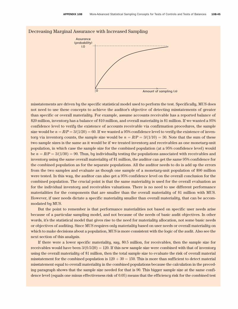
Fourth Pass


smi87468_app10B_10B1-10B67 10B-45 09/15/15 07:17 PM

misstatements are driven by the specific statistical model used to perform the test. Specifically, MUS does not need to use these concepts to achieve the auditor’s objective of detecting misstatements of greater than specific or overall materiality. For example, assume accounts receivable has a reported balance of $20 million, inventory has a balance of $10 million, and overall materiality is $1 million. If we wanted a 95% confidence level to verify the existence of accounts receivable via confirmation procedures, the sample size would be n = R/P = 3/(1/20) = 60. If we wanted a 95% confidence level to verify the existence of inven-tory via inventory counts, the sample size would be n = R/P = 3/(1/10) = 30. Note that the sum of these two sample sizes is the same as it would be if we treated inventory and receivables as one monetary-unit population, in which case the sample size for the combined population (at a 95% confidence level) would be n = R/P = 3/(1/30) = 90. Thus, by individually testing the populations associated with receivables and inventory using the same overall materiality of $1 million, the auditor can get the same 95% confidence for the combined population as for the separate populations. All the auditor needs to do is add up the errors from the two samples and evaluate as though one sample of a monetary-unit population of $90 million were tested. In this way, the auditor can also get a 95% confidence level on the overall conclusion for the combined population. The crucial point is that the same materiality is used for the overall evaluation as for the individual inventory and receivables valuations. There is no need to use different performance materialities for the components that are smaller than the overall materiality of $1 million with MUS. However, if user needs dictate a specific materiality smaller than overall materiality, that can be accom-modated by MUS.

But the point to remember is that performance materialities not based on specific user needs arise because of a particular sampling model, and not because of the needs of basic audit objectives. In other words, it’s the statistical model that gives rise to the need for materiality allocation, not some basic needs or objectives of auditing. Since MUS requires only materiality based on user needs or overall materiality on which to make decisions about a population, MUS is more consistent with the logic of the audit. Also see the next section of this analysis.

If there were a lower specific materiality, say, $0.5 million, for receivables, then the sample size for receivables would have been 3/(0.5/20) = 120. If this new sample size were combined with that of inventory using the overall materiality of $1 million, then the total sample size to evaluate the risk of overall material misstatement for the combined population is 120 + 30 = 150. This is more than sufficient to detect material misstatement equal to overall materiality in the combined populations because the calculation in the preced-ing paragraph shows that the sample size needed for that is 90. This bigger sample size at the same confi-dence level (equals one minus effectiveness risk of 0.05) means that the efficiency risk for the combined test

Decreasing Marginal Assurance with Increased Sampling

Assurance(probability)

1.0

0 Amount of sampling (n)

Fourth Pass


smi87468_app10B_10B1-10B67 10B-46 09/15/15 07:17 PM

has been reduced over the efficiency risk range. Sampling theory predicts you will get some benefit from the increased testing, and, in this case, that benefit takes the form of reduction in efficiency risk, because the effectiveness risk (and confidence level) for the test have been kept at a constant level. However, this is not necessarily the case for all statistical tests when materialities smaller than overall would be required to get the same confidence level for the combined population. MUS can use smaller materialities for specific popu-lations to meet specific user needs, but it does not require this, whereas non-MUS models can require smaller materiality, such as the performance materiality. This requirement has been referred to as materiality alloca-tion. The need for complex materiality allocation rules has been introduced to auditing primarily because of tests based on the normal distribution, further demonstrating how the needs of specific sampling models can affect audit reasoning about evidence gathering.

The calculations in the preceding paragraph also illustrate the chief effect of using smaller performance materialities. Assume that the $0.5 million materiality was a performance materiality instead of a specific (user needs–based) materiality. For example, assume the auditor expected mis-statements of $0.5 million. One way audit firms adjust for the user needs–based materiality to get a performance-based materiality is to subtract the expected misstatements from the user needs–based materiality. In this case, subtract $0.5 million of expected misstatements from the $1 million overall to get $0.5 million of performance materiality, to plan the sample size using performance materiality, as indicated above.

The important distinction to remember is as follows: use a smaller performance materiality to reduce efficiency risk when planning sample sizes, and use overall or specific materiality to control the effective-ness risk. Since efficiency risk can also be controlled by using a higher K value (effectively, more errors expected in the sample), we can summarize most concisely how the major risks and materiality are con-trolled by the following characterization of the MUS formula for sample size:

n = (efficiency riskReffectiveness risk)/(user-based materiality as a proportion of book value)

This formula attempts to concisely summarize the preceding discussion by showing the relationship of the extent of audit work and efficiency risk, effectiveness risk, and user-based materiality. Efficiency risk is affected by the K value chosen. That is why you see efficiency risk as the left-side subscript for R. User-based materiality means the overall or specific materiality of Chapter 5. And effectiveness risk at this user-based materiality is controlled by choosing the confidence level from the R value table. The next section describes how user-based specific materialities relate to the overall materiality in planning an audit.

The Difference between Overall Materiality and Specific Materiality Based on User Needs

According to CAS 320.10–11, overall materiality is for financial statements as a whole (i.e., overall conclu-sion of 5025), versus performance materialities, which are lesser amounts that would affect some users for particular transactions, account balances, or disclosures, a qualified opinion would normally be used if misstatements exceed performance materiality, and an adverse opinion or disclaimer would be used for overall materiality.

In order to better understand the distinction between overall materiality and performance materiality based on user needs (i.e., what we call specific materiality), assume there are a total of n users of the finan-cial statements of an auditee, and you can also assume that each user has a different (performance) mate-riality Mi. Next assume you rank these materialities from smallest to largest so that M1 less than or equal to M2 and so on until Mn, which is the largest materiality. The easiest way to understand CAS 320 is by the way the auditor selects overall materiality, Mo, relative to Mi, where i is greater than zero. A simple approach is to pick Mo = M1. Under this approach the auditor sets overall materiality so that it meets the needs of the

Fourth Pass


smi87468_app10B_10B1-10B67 10B-47 09/15/15 07:17 PM

most demanding user. Of course, by doing so the auditor also automatically satisfies the materiality needs of less demanding users. But this occurs at the cost of additional work on accounts where the additional work is not needed. But what suffers is audit efficiency, not audit effectiveness. Thus, using the smallest performance materiality, M1, for the entire audit results in possibly too much audit work but does not reduce audit effectiveness.

If the auditor picks Mo to be greater than M1, then there is a difference between overall materiality and performance materiality. Under these conditions the auditor does less work for accounts that use the per-formance materiality. You see how this works in practice with this Application Case.

Auditing as a Bayesian Reasoning Process

Perhaps the most important influence on audit reasoning is the Bayesian view of evidence (i.e., use of Bayes’ theorem and Bayesian logic to evaluate the evidence). Auditors tend to adopt the Bayesian phi-losophy. The important thing about this view for auditors is that under the Bayesian view of evidence the auditor interprets statistical test results as statements about the probability of material misstatement. If the only audit evidence is the MUS statistical test, and if the auditor accepts the population, then under the Bayesian perspective the auditor can interpret the confidence level as the probability of less than material misstatement and the effectiveness risk as the probability of material misstatement. This view permeates audit reasoning to the point of being reflected in the audit risk model. For our purposes, the importance of the Bayesian view is that it allows the assurance to correspond to the confidence level and the effectiveness risk to the probability of material misstatement. Under this Bayesian view, it can be shown that decision rule (1) is equivalent to the following:

Decision Rule (2):

If the probability of material misstatement is greater than the acceptable risk, then reject; otherwise, accept the recorded amount.

The interesting aspect of decision rule (2) is that it can be applied to all types of risk, not just sampling risk. In particular, this decision rule can be applied to the components of the audit risk model and to the accounting risk concept. Thus, decision rule (2) provides a means for introducing consistency in reasoning for financial reporting involving estimates as well as for other auditing issues. Consistency in reasoning is important to good logic, and it is best that audit reasoning processes be defended as logical. Inconsisten-cies in reasoning indicate that there is a contradiction, which, in turn, indicates flawed and illogical reason-ing. It would be very difficult for an auditor to defend his or her work if the courts or the Canadian Public Accountability Board (CPAB) could show that there is an unresolved contradiction. In fact, philosophers have shown that contradictions can be used to represent lying (i.e., stated belief contradicts actual belief).

Chapter 4 distinguishes accounting deficiencies from audit deficiencies. If auditors are to deal with these deficiencies consistently, then a reasoning process like decision rule (2) is one way of doing so. Note that since decision rule (2) focuses on risks, it is fully consistent with risk-based auditing and offers a way to deal with accounting risks of financial reporting as well as audit risk. We illustrate this in the Application Cases of Chapters 19 and 21 (available on Connect), where suitable criteria for financial reporting are discussed.

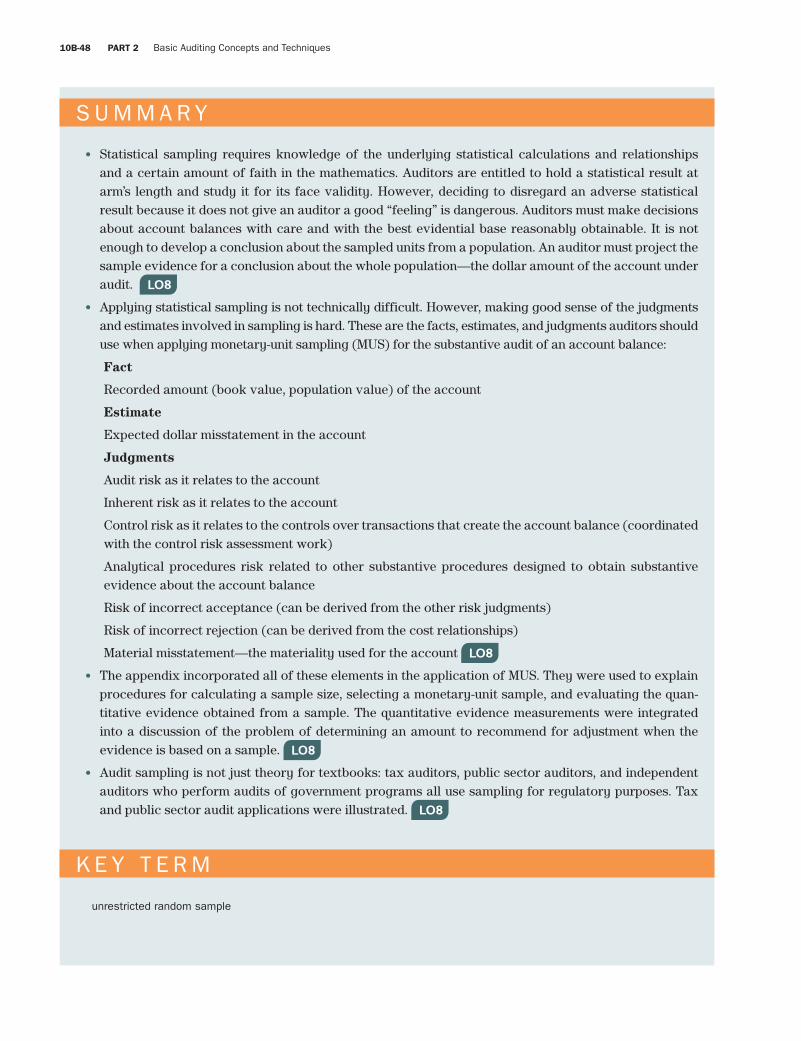
Fourth Pass


smi87468_app10B_10B1-10B67 10B-48 09/15/15 07:17 PM

S U M M A R Y

• Statistical sampling requires knowledge of the underlying statistical calculations and relationships and a certain amount of faith in the mathematics. Auditors are entitled to hold a statistical result at arm’s length and study it for its face validity. However, deciding to disregard an adverse statistical result because it does not give an auditor a good “feeling” is dangerous. Auditors must make decisions about account balances with care and with the best evidential base reasonably obtainable. It is not enough to develop a conclusion about the sampled units from a population. An auditor must project the sample evidence for a conclusion about the whole population—the dollar amount of the account under audit. LO8

• Applying statistical sampling is not technically difficult. However, making good sense of the judgments and estimates involved in sampling is hard. These are the facts, estimates, and judgments auditors should use when applying monetary-unit sampling (MUS) for the substantive audit of an account balance:

Fact

Recorded amount (book value, population value) of the account

Estimate

Expected dollar misstatement in the account

Judgments

Audit risk as it relates to the account

Inherent risk as it relates to the account

Control risk as it relates to the controls over transactions that create the account balance (coordinated with the control risk assessment work)

Analytical procedures risk related to other substantive procedures designed to obtain substantive evidence about the account balance

Risk of incorrect acceptance (can be derived from the other risk judgments)

Risk of incorrect rejection (can be derived from the cost relationships)

Material misstatement—the materiality used for the account LO8

• The appendix incorporated all of these elements in the application of MUS. They were used to explain procedures for calculating a sample size, selecting a monetary-unit sample, and evaluating the quan-titative evidence obtained from a sample. The quantitative evidence measurements were integrated into a discussion of the problem of determining an amount to recommend for adjustment when the evidence is based on a sample. LO8

• Audit sampling is not just theory for textbooks: tax auditors, public sector auditors, and independent auditors who perform audits of government programs all use sampling for regulatory purposes. Tax and public sector audit applications were illustrated. LO8

K E Y T E R M

unrestricted random sample

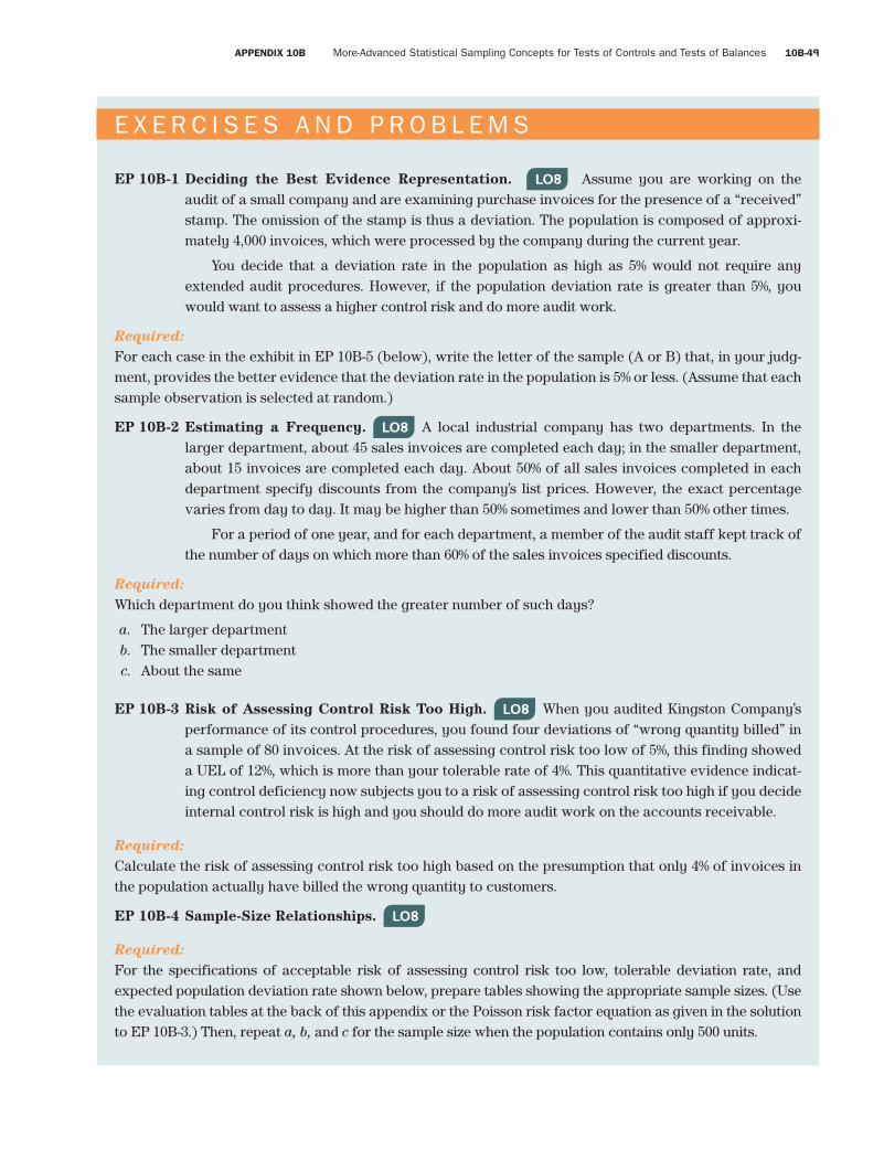
Fourth Pass


smi87468_app10B_10B1-10B67 10B-49 09/15/15 07:17 PM

E X E R C I S E S A N D P R O B L E M S

EP 10B-1 Deciding the Best Evidence Representation. LO8 Assume you are working on the audit of a small company and are examining purchase invoices for the presence of a “received” stamp. The omission of the stamp is thus a deviation. The population is composed of approxi-mately 4,000 invoices, which were processed by the company during the current year.

You decide that a deviation rate in the population as high as 5% would not require any extended audit procedures. However, if the population deviation rate is greater than 5%, you would want to assess a higher control risk and do more audit work.

Required:For each case in the exhibit in EP 10B-5 (below), write the letter of the sample (A or B) that, in your judg-ment, provides the better evidence that the deviation rate in the population is 5% or less. (Assume that each sample observation is selected at random.)

EP 10B-2 Estimating a Frequency. LO8 A local industrial company has two departments. In the larger department, about 45 sales invoices are completed each day; in the smaller department, about 15 invoices are completed each day. About 50% of all sales invoices completed in each department specify discounts from the company’s list prices. However, the exact percentage varies from day to day. It may be higher than 50% sometimes and lower than 50% other times.

For a period of one year, and for each department, a member of the audit staff kept track of the number of days on which more than 60% of the sales invoices specified discounts.

Required:Which department do you think showed the greater number of such days?

a. The larger department b. The smaller department c. About the same

EP 10B-3 Risk of Assessing Control Risk Too High. LO8 When you audited Kingston Company’s performance of its control procedures, you found four deviations of “wrong quantity billed” in a sample of 80 invoices. At the risk of assessing control risk too low of 5%, this finding showed a UEL of 12%, which is more than your tolerable rate of 4%. This quantitative evidence indicat-ing control deficiency now subjects you to a risk of assessing control risk too high if you decide internal control risk is high and you should do more audit work on the accounts receivable.

Required:Calculate the risk of assessing control risk too high based on the presumption that only 4% of invoices in the population actually have billed the wrong quantity to customers.

EP 10B-4 Sample-Size Relationships. LO8

Required:For the specifications of acceptable risk of assessing control risk too low, tolerable deviation rate, and expected population deviation rate shown below, prepare tables showing the appropriate sample sizes. (Use the evaluation tables at the back of this appendix or the Poisson risk factor equation as given in the solution to EP 10B-3.) Then, repeat a, b, and c for the sample size when the population contains only 500 units.

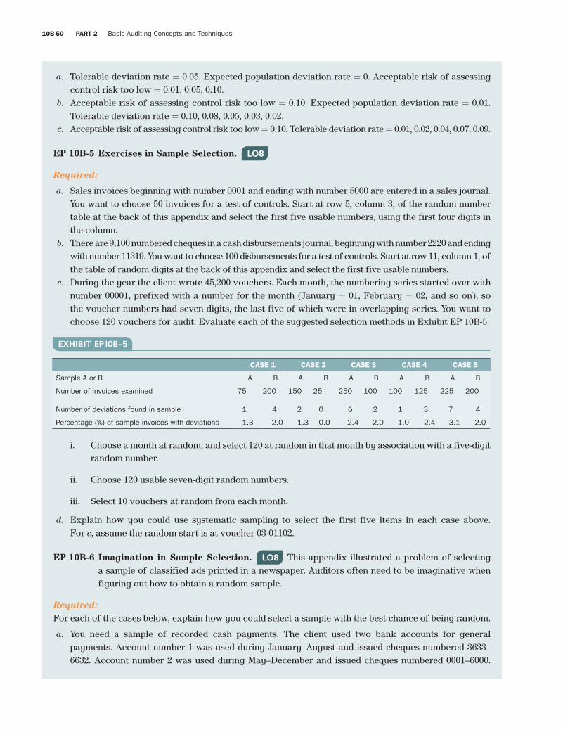
Fourth Pass


smi87468_app10B_10B1-10B67 10B-50 09/15/15 07:17 PM

a. Tolerable deviation rate = 0.05. Expected population deviation rate = 0. Acceptable risk of assessing control risk too low = 0.01, 0.05, 0.10.

b. Acceptable risk of assessing control risk too low = 0.10. Expected population deviation rate = 0.01. Tolerable deviation rate = 0.10, 0.08, 0.05, 0.03, 0.02.

c. Acceptable risk of assessing control risk too low = 0.10. Tolerable deviation rate = 0.01, 0.02, 0.04, 0.07, 0.09.

EP 10B-5 Exercises in Sample Selection. LO8

Required:

a. Sales invoices beginning with number 0001 and ending with number 5000 are entered in a sales journal. You want to choose 50 invoices for a test of controls. Start at row 5, column 3, of the random number table at the back of this appendix and select the first five usable numbers, using the first four digits in the column.

b. There are 9,100 numbered cheques in a cash disbursements journal, beginning with number 2220 and ending with number 11319. You want to choose 100 disbursements for a test of controls. Start at row 11, column 1, of the table of random digits at the back of this appendix and select the first five usable numbers.

c. During the year the client wrote 45,200 vouchers. Each month, the numbering series started over with number 00001, prefixed with a number for the month (January = 01, February = 02, and so on), so the voucher numbers had seven digits, the last five of which were in overlapping series. You want to choose 120 vouchers for audit. Evaluate each of the suggested selection methods in Exhibit EP 10B-5.

i. Choose a month at random, and select 120 at random in that month by association with a five-digit random number.

ii. Choose 120 usable seven-digit random numbers.

iii. Select 10 vouchers at random from each month.

d. Explain how you could use systematic sampling to select the first five items in each case above. For c, assume the random start is at voucher 03-01102.

EP 10B-6 Imagination in Sample Selection. LO8 This appendix illustrated a problem of selecting a sample of classified ads printed in a newspaper. Auditors often need to be imaginative when figuring out how to obtain a random sample.

Required:For each of the cases below, explain how you could select a sample with the best chance of being random.

a. You need a sample of recorded cash payments. The client used two bank accounts for general payments. Account number 1 was used during January–August and issued cheques numbered 3633–6632. Account number 2 was used during May–December and issued cheques numbered 0001–6000.

CASE 1 CASE 2 CASE 3 CASE 4 CASE 5

Sample A or B A B A B A B A B A B

Number of invoices examined 75 200 150 25 250 100 100 125 225 200

Number of deviations found in sample 1 4 2 0 6 2 1 3 7 4

Percentage (%) of sample invoices with deviations 1.3 2.0 1.3 0.0 2.4 2.0 1.0 2.4 3.1 2.0

EXHIBIT EP10B–5

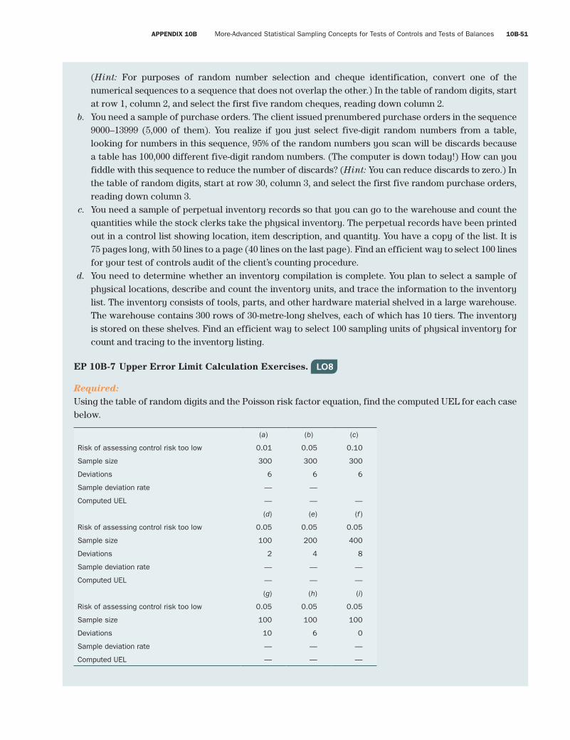
Fourth Pass


smi87468_app10B_10B1-10B67 10B-51 09/15/15 07:17 PM

(Hint: For purposes of random number selection and cheque identification, convert one of the numerical sequences to a sequence that does not overlap the other.) In the table of random digits, start at row 1, column 2, and select the first five random cheques, reading down column 2.

b. You need a sample of purchase orders. The client issued prenumbered purchase orders in the sequence 9000–13999 (5,000 of them). You realize if you just select five-digit random numbers from a table, looking for numbers in this sequence, 95% of the random numbers you scan will be discards because a table has 100,000 different five-digit random numbers. (The computer is down today!) How can you fiddle with this sequence to reduce the number of discards? (Hint: You can reduce discards to zero.) In the table of random digits, start at row 30, column 3, and select the first five random purchase orders, reading down column 3.

c. You need a sample of perpetual inventory records so that you can go to the warehouse and count the quantities while the stock clerks take the physical inventory. The perpetual records have been printed out in a control list showing location, item description, and quantity. You have a copy of the list. It is 75 pages long, with 50 lines to a page (40 lines on the last page). Find an efficient way to select 100 lines for your test of controls audit of the client’s counting procedure.

d. You need to determine whether an inventory compilation is complete. You plan to select a sample of physical locations, describe and count the inventory units, and trace the information to the inventory list. The inventory consists of tools, parts, and other hardware material shelved in a large warehouse. The warehouse contains 300 rows of 30-metre-long shelves, each of which has 10 tiers. The inventory is stored on these shelves. Find an efficient way to select 100 sampling units of physical inventory for count and tracing to the inventory listing.

EP 10B-7 Upper Error Limit Calculation Exercises. LO8

Required:Using the table of random digits and the Poisson risk factor equation, find the computed UEL for each case below.

(a) (b) (c)

Risk of assessing control risk too low 0.01 0.05 0.10

Sample size 300 300 300

Deviations 6 6 6

Sample deviation rate — —

Computed UEL — — —

(d) (e) (f)



Deviations 2 4 8

Sample deviation rate — — —


(g) (h) (i)



Deviations 10 6 0

Sample deviation rate — — —


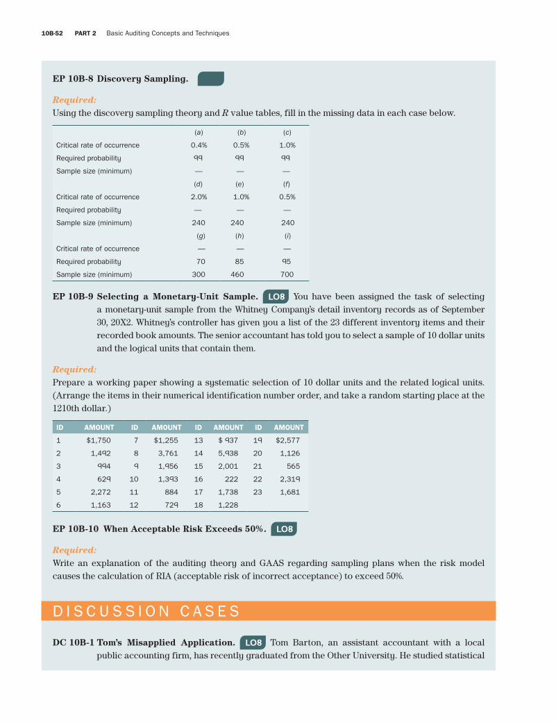
Fourth Pass


smi87468_app10B_10B1-10B67 10B-52 09/15/15 07:17 PM

EP 10B-8 Discovery Sampling. LO8

Required:Using the discovery sampling theory and R value tables, fill in the missing data in each case below.

(a) (b) (c)

Critical rate of occurrence 0.4% 0.5% 1.0%

Required probability 99 99 99

Sample size (minimum) — — —

(d) (e) (f)

Critical rate of occurrence 2.0% 1.0% 0.5%

Required probability — — —

Sample size (minimum) 240 240 240

(g) (h) (i)

Critical rate of occurrence — — —

Required probability 70 85 95

Sample size (minimum) 300 460 700

EP 10B-9 Selecting a Monetary-Unit Sample. LO8 You have been assigned the task of selecting a monetary-unit sample from the Whitney Company’s detail inventory records as of September 30, 20X2. Whitney’s controller has given you a list of the 23 different inventory items and their recorded book amounts. The senior accountant has told you to select a sample of 10 dollar units and the logical units that contain them.

Required:Prepare a working paper showing a systematic selection of 10 dollar units and the related logical units. (Arrange the items in their numerical identification number order, and take a random starting place at the 1210th dollar.)

ID AMOUNT ID AMOUNT ID AMOUNT ID AMOUNT

1 $1,750 7 $1,255 13 $ 937 19 $2,577

2 1,492 8 3,761 14 5,938 20 1,126

3 994 9 1,956 15 2,001 21 565

4 629 10 1,393 16 222 22 2,319

5 2,272 11 884 17 1,738 23 1,681

6 1,163 12 729 18 1,228

EP 10B-10 When Acceptable Risk Exceeds 50%. LO8

Required:Write an explanation of the auditing theory and GAAS regarding sampling plans when the risk model causes the calculation of RIA (acceptable risk of incorrect acceptance) to exceed 50%.

D I S C U S S I O N C A S E S

DC 10B-1 Tom’s Misapplied Application. LO8 Tom Barton, an assistant accountant with a local public accounting firm, has recently graduated from the Other University. He studied statistical

Fourth Pass


smi87468_app10B_10B1-10B67 10B-53 09/15/15 07:17 PM

sampling for auditing in university and wants to impress his employers with his knowledge of modern auditing methods.

He decided to select a random sample of payroll cheques for the test of controls, using a tolerable rate of 5% and an acceptable risk of assessing control risk too low of 5%. The senior accountant told Tom that 2% of the cheques audited last year had one or more errors in the cal-culation of net pay. Tom decided to audit 100 random cheques. Since supervisory personnel had larger paycheques than production workers, he selected 60 of the larger cheques and 40 of the others. He was very careful to see that the selections of 60 from the April payroll register and 40 from the August payroll register were random.

The audit of this sample yielded two deviations, exactly the 2% rate experienced last year. The first was the deduction of federal income taxes based on two exemptions for a supervisory employee. The other was payment to a production employee at a rate for a job classification one grade lower than his actual job. The worker had been promoted the week before, and Tom found that in the next payroll he was paid at the higher correct rate.

When he evaluated this evidence, Tom decided that these two findings were really not con-trol deviations at all. The withholding of too much tax did not affect the expense accounts, and the proper rate was paid the production worker as soon as the clerk caught up with his change orders. Tom decided that having found zero deviations in a sample of 100, the computed upper limit at 5% risk of assessing control risk too low was 3%, which easily satisfied his predetermined criterion.

The senior accountant was impressed. Last year, he had audited 15 cheques from each month, and Tom’s work represented a significant time savings. The reviewing partner on the audit was also impressed because he had never thought that statistical sampling could be so efficient, and that was the reason he had never studied the method.

Required:Identify and explain the mistakes made by Tom and the others.

DC 10B-2 Determine Sample Size for a Test of Controls. LO8 N. Wolfe, PA, is planning the audit of Goodwin Manufacturing Company’s inventory. Wolfe plans to audit the inventory by selecting a sample of items for physical observation and counting, followed by price testing. The price testing part of the work takes a large portion of the time on each sampling unit because the company’s costing method is complex. The estimated cost of auditing each sampling unit in this substantive balance-audit sample is estimated at $25.

Because this detailed substantive work is expensive, Wolfe would like to minimize the sample size by assessing a low control risk. She decided that control over accurate pricing of purchases (additions to the inventory) would be the most appropriate control attribute. The reasoning is that inventory balance misstatements could arise from either or both of miscounting or erro-neous pricing and costing calculations. If the basic purchase pricing were accurate, then the inventory count accuracy and the difficult inventory costing calculations would be the remain-ing source for error and audit attention. The estimated cost to audit a purchase transaction for pricing accuracy is estimated to be $12. She thinks the client’s staff makes few, if any, errors in pricing the purchase transactions.

For the audit of the inventory balance, Wolfe accepted the accounting firm’s policy of set-ting audit risk at 0.05. Since business activity in the client company had been hectic lately, she decided to be conservative and set inherent risk at 1.0. However, certain analytical procedures will be performed by comparing the inventory balance to prior years, the company budget, and

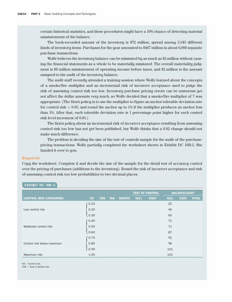
Fourth Pass


smi87468_app10B_10B1-10B67 10B-54 09/15/15 07:17 PM

certain historical statistics, and these procedures might have a 10% chance of detecting material misstatements of the balance.

The book-recorded amount of the inventory is $72 million, spread among 3,345 different kinds of inventory items. Purchases for the year amounted to $467 million in about 6,000 separate purchase transactions.

Wolfe believes the inventory balance can be misstated by as much as $2 million without caus-ing the financial statements as a whole to be materially misstated. The overall materiality judg-ment is $8 million misstatement of operating income before taxes, and $2 million is the amount assigned to the audit of the inventory balance.

The audit staff recently attended a training session where Wolfe learned about the concepts of a smoke/fire multiplier and an incremental risk of incorrect acceptance used to judge the risk of assessing control risk too low. Inventory purchase pricing errors can be numerous yet not affect the dollar amounts very much, so Wolfe decided that a smoke/fire multiplier of 7 was appropriate. (The firm’s policy is to use the multiplier to figure an anchor tolerable deviation rate for control risk = 0.05, and round the anchor up to 1% if the multiplier produces an anchor less than 1%. After that, each tolerable deviation rate is 1 percentage point higher for each control risk level increment of 0.05.)

The firm’s policy about an incremental risk of incorrect acceptance resulting from assessing control risk too low has not yet been published, but Wolfe thinks that a 0.02 change should not make much difference.

The problem is deciding the size of the test of controls sample for the audit of the purchase-pricing transactions. Wolfe partially completed the worksheet shown in Exhibit DC 10B-2. She handed it over to you.

Required:Copy the worksheet. Complete it and decide the size of the sample for the detail test of accuracy control over the pricing of purchases (additions to the inventory). Round the risk of incorrect acceptance and risk of assessing control risk too low probabilities to two decimal places.

CR = Control risk.TDR = Test of details risk.

TEST OF CONTROL BALANCE-AUDIT

CONTROL RISK CATEGORIES CR TDR RIA RACRTL N[C] COST N[S] COST TOTAL

Low control risk

0.10

0.20

0.30

25

46

60


0.40

0.50

0.60

71

71

87

Control risk below maximum

0.70

0.80

0.90

91

96

101

Maximum risk 1.00 101

EXHIBIT DC 10B–2

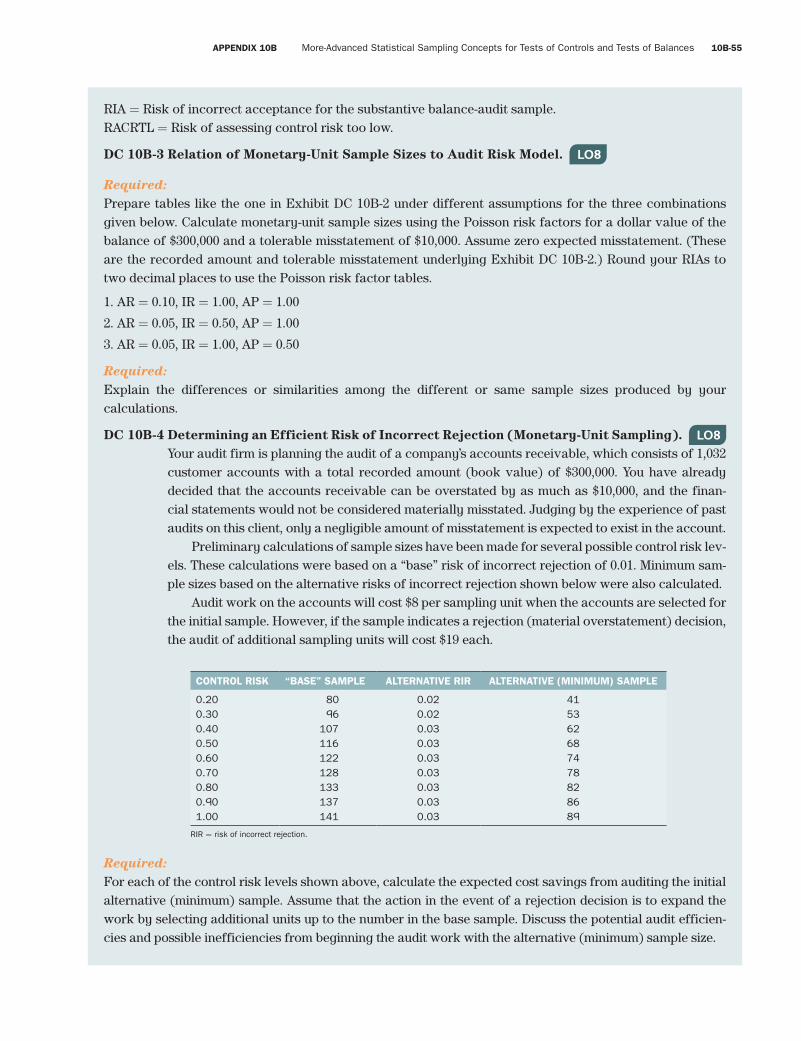
Fourth Pass


smi87468_app10B_10B1-10B67 10B-55 09/15/15 07:17 PM

RIA = Risk of incorrect acceptance for the substantive balance-audit sample.RACRTL = Risk of assessing control risk too low.

DC 10B-3 Relation of Monetary-Unit Sample Sizes to Audit Risk Model. LO8

Required:Prepare tables like the one in Exhibit DC 10B-2 under different assumptions for the three combinations given below. Calculate monetary-unit sample sizes using the Poisson risk factors for a dollar value of the balance of $300,000 and a tolerable misstatement of $10,000. Assume zero expected misstatement. (These are the recorded amount and tolerable misstatement underlying Exhibit DC 10B-2.) Round your RIAs to two decimal places to use the Poisson risk factor tables.

1. AR = 0.10, IR = 1.00, AP = 1.00

2. AR = 0.05, IR = 0.50, AP = 1.00

3. AR = 0.05, IR = 1.00, AP = 0.50

Required:Explain the differences or similarities among the different or same sample sizes produced by your calculations.

DC 10B-4 Determining an Efficient Risk of Incorrect Rejection (Monetary-Unit Sampling). LO8 Your audit firm is planning the audit of a company’s accounts receivable, which consists of 1,032 customer accounts with a total recorded amount (book value) of $300,000. You have already decided that the accounts receivable can be overstated by as much as $10,000, and the finan-cial statements would not be considered materially misstated. Judging by the experience of past audits on this client, only a negligible amount of misstatement is expected to exist in the account.

Preliminary calculations of sample sizes have been made for several possible control risk lev-els. These calculations were based on a “base” risk of incorrect rejection of 0.01. Minimum sam-ple sizes based on the alternative risks of incorrect rejection shown below were also calculated.

Audit work on the accounts will cost $8 per sampling unit when the accounts are selected for the initial sample. However, if the sample indicates a rejection (material overstatement) decision, the audit of additional sampling units will cost $19 each.

Required:For each of the control risk levels shown above, calculate the expected cost savings from auditing the initial alternative (minimum) sample. Assume that the action in the event of a rejection decision is to expand the work by selecting additional units up to the number in the base sample. Discuss the potential audit efficien-cies and possible inefficiencies from beginning the audit work with the alternative (minimum) sample size.

CONTROL RISK “BASE” SAMPLE ALTERNATIVE RIR ALTERNATIVE (MINIMUM) SAMPLE

0.200.300.400.500.600.700.800.901.00

8096

107116122128133137141

0.020.020.030.030.030.030.030.030.03

415362687478828689

RIR = risk of incorrect rejection.

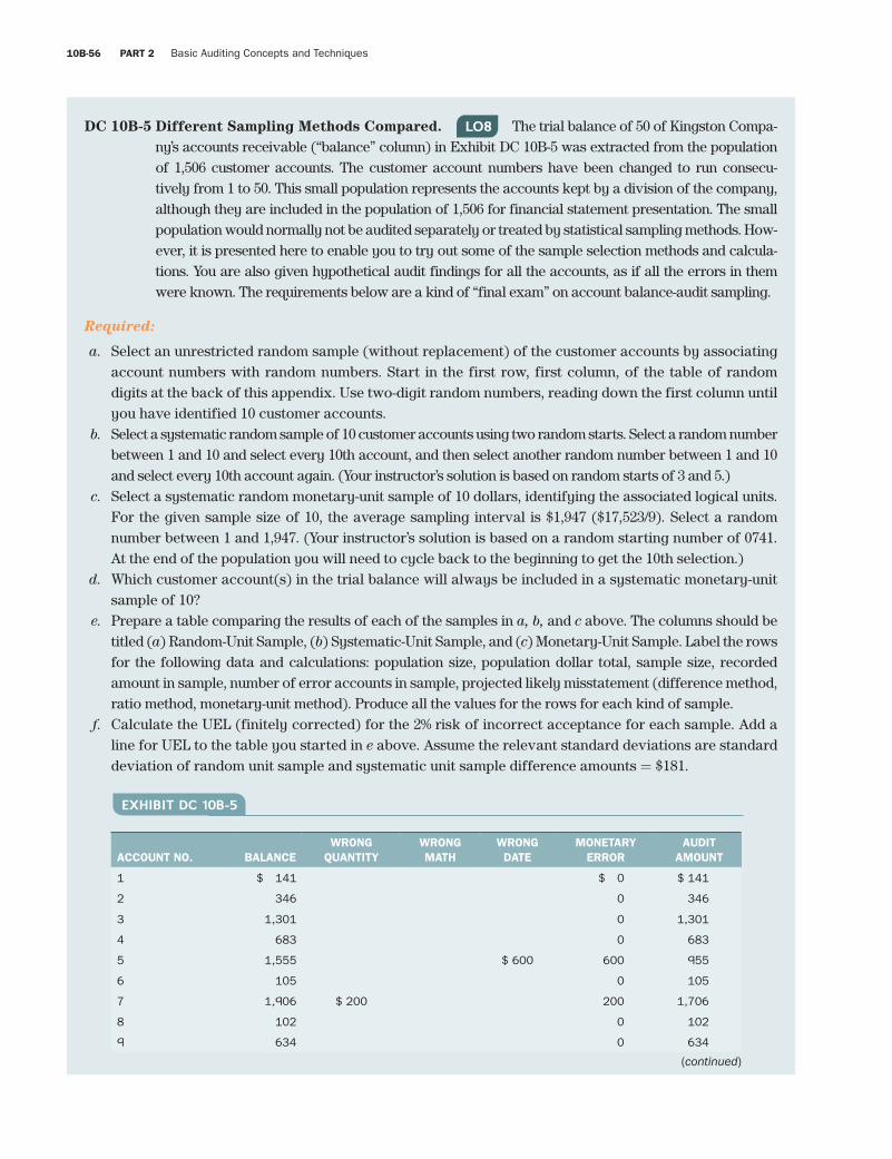
Fourth Pass


smi87468_app10B_10B1-10B67 10B-56 09/15/15 07:17 PM

DC 10B-5 Different Sampling Methods Compared. LO8 The trial balance of 50 of Kingston Compa-ny’s accounts receivable (“balance” column) in Exhibit DC 10B-5 was extracted from the population of 1,506 customer accounts. The customer account numbers have been changed to run consecu-tively from 1 to 50. This small population represents the accounts kept by a division of the company, although they are included in the population of 1,506 for financial statement presentation. The small population would normally not be audited separately or treated by statistical sampling methods. How-ever, it is presented here to enable you to try out some of the sample selection methods and calcula-tions. You are also given hypothetical audit findings for all the accounts, as if all the errors in them were known. The requirements below are a kind of “final exam” on account balance-audit sampling.

Required:

a. Select an unrestricted random sample (without replacement) of the customer accounts by associating account numbers with random numbers. Start in the first row, first column, of the table of random digits at the back of this appendix. Use two-digit random numbers, reading down the first column until you have identified 10 customer accounts.

b. Select a systematic random sample of 10 customer accounts using two random starts. Select a random number between 1 and 10 and select every 10th account, and then select another random number between 1 and 10 and select every 10th account again. (Your instructor’s solution is based on random starts of 3 and 5.)

c. Select a systematic random monetary-unit sample of 10 dollars, identifying the associated logical units. For the given sample size of 10, the average sampling interval is $1,947 ($17,523/9). Select a random number between 1 and 1,947. (Your instructor’s solution is based on a random starting number of 0741. At the end of the population you will need to cycle back to the beginning to get the 10th selection.)

d. Which customer account(s) in the trial balance will always be included in a systematic monetary-unit sample of 10?

e. Prepare a table comparing the results of each of the samples in a, b, and c above. The columns should be titled (a) Random-Unit Sample, (b) Systematic-Unit Sample, and (c) Monetary-Unit Sample. Label the rows for the following data and calculations: population size, population dollar total, sample size, recorded amount in sample, number of error accounts in sample, projected likely misstatement (difference method, ratio method, monetary-unit method). Produce all the values for the rows for each kind of sample.

f. Calculate the UEL (finitely corrected) for the 2% risk of incorrect acceptance for each sample. Add a line for UEL to the table you started in e above. Assume the relevant standard deviations are standard deviation of random unit sample and systematic unit sample difference amounts = $181.

ACCOUNT NO. BALANCEWRONG

QUANTITYWRONG MATH

WRONG DATE

MONETARY ERROR

AUDIT AMOUNT

1 $ 141 $ 0 $ 141

2 346 0 346

3 1,301 0 1,301

4 683 0 683

5 1,555 $ 600 600 955

6 105 0 105

7 1,906 $ 200 200 1,706

8 102 0 102

9 634 0 634

EXHIBIT DC 10B-5

(continued)

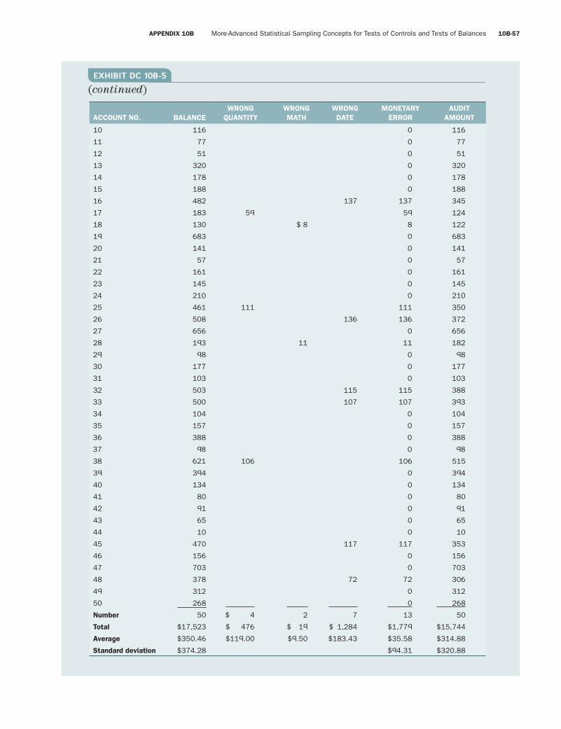
Fourth Pass


smi87468_app10B_10B1-10B67 10B-57 09/15/15 07:17 PM

ACCOUNT NO. BALANCEWRONG

QUANTITYWRONG MATH

WRONG DATE

MONETARY ERROR

AUDIT AMOUNT

10 116 0 116

11 77 0 77

12 51 0 51

13 320 0 320

14 178 0 178

15 188 0 188

16 482 137 137 345

17 183 59 59 124

18 130 $ 8 8 122

19 683 0 683

20 141 0 141

21 57 0 57

22 161 0 161

23 145 0 145

24 210 0 210

25 461 111 111 350

26 508 136 136 372

27 656 0 656

28 193 11 11 182

29 98 0 98

30 177 0 177

31 103 0 103

32 503 115 115 388

33 500 107 107 393

34 104 0 104

35 157 0 157

36 388 0 388

37 98 0 98

38 621 106 106 515

39 394 0 394

40 134 0 134

41 80 0 80

42 91 0 91

43 65 0 65

44 10 0 10

45 470 117 117 353

46 156 0 156

47 703 0 703

48 378 72 72 306

49 312 0 312

50 268 0 268

Number 50 $ 4 2 7 13 50

Total $17,523 $ 476 $ 19 $ 1,284 $1,779 $15,744

Average $350.46 $119.00 $9.50 $183.43 $35.58 $314.88

Standard deviation $374.28 $94.31 $320.88

EXHIBIT DC 10B-5

(continued)

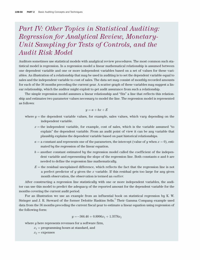
Fourth Pass


smi87468_app10B_10B1-10B67 10B-58 09/15/15 07:17 PM

Part IV: Other Topics in Statistical Auditing: Regression for Analytical Review, Monetary- Unit Sampling for Tests of Controls, and the Audit Risk ModelAuditors sometimes use statistical models with analytical review procedures. The most common such sta-tistical model is regression. In a regression model a linear mathematical relationship is assumed between one dependent variable and one or more independent variables based on a set of values for these vari-ables. An illustration of a relationship that may be used in auditing is to set the dependent variable equal to sales and the independent variable to cost of sales. The data set may consist of monthly recorded amounts for each of the 36 months preceding the current year. A scatter graph of these variables may suggest a lin-ear relationship, which the auditor might exploit to get audit assurance from such a relationship.

The simple regression model assumes a linear relationship and “fits” a line that reflects this relation-ship and estimates two parameter values necessary to model the line. The regression model is represented as follows:

y = a + bx + E

where y = the dependent variable values, for example, sales values, which vary depending on the independent variable.

x = the independent variable, for example, cost of sales, which is the variable assumed “to explain” the dependent variable. From an audit point of view it can be any variable that plausibly explains the dependent variable based on past historical relationships.

a = a constant and represents one of the parameters, the intercept (value of y when x = 0), esti-mated by the regression of the linear equation.

b = another constant estimated by the regression model called the coefficient of the indepen-dent variable and representing the slope of the regression line. Both constants a and b are needed to define the regression line mathematically.

E = the residual unexplained difference, which reflects the fact that the regression line is not a perfect predictor of y given the x variable. If this residual gets too large for any given month observation, the observation is termed an outlier.

After constructing a regression line statistically with one or more independent variables, the audi-tor can use this model to predict the adequacy of the reported amount for the dependent variable for the months covering the current audit period.

For an illustration we use an example from an influential book on statistical regression by K. W. Stringer and J. R. Steward of the former Deloitte Haskins Sells.7 Their Gamma Company example used data from the 36 months preceding the current fiscal year to estimate a linear equation using regression of the following form:

y =-366.46 + 0.8906x1 + 1.3578x2

where y here represents revenues for a software firm,x1 = programming hours at standard, andx2 = expenses

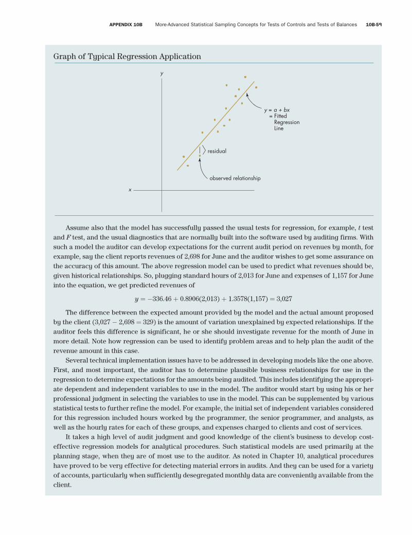
Fourth Pass


smi87468_app10B_10B1-10B67 10B-59 09/15/15 07:17 PM

Assume also that the model has successfully passed the usual tests for regression, for example, t test and F test, and the usual diagnostics that are normally built into the software used by auditing firms. With such a model the auditor can develop expectations for the current audit period on revenues by month, for example, say the client reports revenues of 2,698 for June and the auditor wishes to get some assurance on the accuracy of this amount. The above regression model can be used to predict what revenues should be, given historical relationships. So, plugging standard hours of 2,013 for June and expenses of 1,157 for June into the equation, we get predicted revenues of

y = −336.46 + 0.8906(2,013) + 1.3578(1,157) = 3,027

The difference between the expected amount provided by the model and the actual amount proposed by the client (3,027 − 2,698 = 329) is the amount of variation unexplained by expected relationships. If the auditor feels this difference is significant, he or she should investigate revenue for the month of June in more detail. Note how regression can be used to identify problem areas and to help plan the audit of the revenue amount in this case.

Several technical implementation issues have to be addressed in developing models like the one above. First, and most important, the auditor has to determine plausible business relationships for use in the regression to determine expectations for the amounts being audited. This includes identifying the appropri-ate dependent and independent variables to use in the model. The auditor would start by using his or her professional judgment in selecting the variables to use in the model. This can be supplemented by various statistical tests to further refine the model. For example, the initial set of independent variables considered for this regression included hours worked by the programmer, the senior programmer, and analysts, as well as the hourly rates for each of these groups, and expenses charged to clients and cost of services.

It takes a high level of audit judgment and good knowledge of the client’s business to develop cost-effective regression models for analytical procedures. Such statistical models are used primarily at the planning stage, when they are of most use to the auditor. As noted in Chapter 10, analytical procedures have proved to be very effective for detecting material errors in audits. And they can be used for a variety of accounts, particularly when sufficiently desegregated monthly data are conveniently available from the client.

y

x

y = a + bx = Fitted Regression Line

residual

observed relationship

Graph of Typical Regression Application

Fourth Pass


smi87468_app10B_10B1-10B67 10B-60 09/15/15 07:17 PM

However, caution is advisable since research has also shown that while statistical analytical review can be used to provide some audit assurance for client accounts, it should not be used to provide a high level or the sole amount of assurance for anything other than immaterial amounts.

Another caution is that because of the sensitivity of the regression results to materiality, the planned level of assurance (the confidence level), and the need to use the negative approach, auditors need to develop a special interface in applying regression models to audit practice. In other words, you cannot just take a regression package available from, say, Microsoft Excel and apply it to your audit data. Keep in mind that audit assurance is related to 1 – RIA, not 1 – RIR. Specifically, in most scientific applications the null hypothesis relates to there being no difference because the scientist is usually interested in the effects of some experimental treatment. In auditing, because the crucial null hypothesis assumes there is a material difference, the confidence level is the complement of the opposite risk that is normally used in the sciences. Specifically, in the sciences (and therefore in most statistical tables), the positive approach is used rather than the negative approach that is relevant to the auditor.

As a result, special adjustments normally need to be made for classical statistical estimators, including the regression model. That is why audit firms have developed a special audit interface to be used with the regression models. And you should be aware of the need for such an interface before applying off-the-shelf regression packages to audit applications. In fact, it is far better to obtain a package specially tailored for auditor use. Most of the large firms already have such packages, making the use of statistical analytical procedures very feasible.

Research has shown that the negative approach for analytical review in auditing is preferred to the positive approach in controlling both efficiency and effectiveness risks.8

Monetary-Unit Sampling for Tests of ControlsAlthough we have noted that MUS formulas can be used for tests of controls applications, we implicitly assumed in all our illustrations that the test of controls sampling was based on physical-unit selection. Some auditors argue that a more appropriate way of evaluating controls is to use MUS rather than physical-unit selection. This is because automatic stratification of the population results from MUS, so the evaluation of controls can be based on the maximum proportion of dollars (rather than the maximum proportion of physical units) in the population that is likely to contain errors. Research has shown that compliance devi-ation rates per recorded dollar can be substantially different from compliance deviation rates for physical units, such as sales invoices and shipping documents.

For example, in the stratification example in Chapter 10, compliance deviations for strata 3, 4, 5 may be much higher than for the high-valued items in strata 1 and 2. The auditor can incorporate such differ-ences judgmentally or let the MUS sampling technique automatically account for this effect in evaluat-ing controls. Note that such differences in controls for different strata could affect auditor strategies, as noted in Exhibit 10–5. In fact, we can take the position that unstratified physical-unit sampling for attri-butes ignores possible differing strengths of controls based on the value of items recorded—unstratified physical-unit sampling for tests of controls implicitly assumes controls are equally strong for high-value items and low-value items. Limited empirical evidence on this issue suggests that this is not the case in practice. Nevertheless, unstratified physical units is the most commonly used method in current practice. A Canadian research study has called for a change in this practice and increased reliance on MUS for control testing.9 As the importance of auditor reports on internal controls increases, perhaps this issue will gain increasing prominence.

Fourth Pass


smi87468_app10B_10B1-10B67 10B-61 09/15/15 07:17 PM

For example, the increasingly important concept of continuous auditing allows a way to calculate sample size and sampling interval without knowing the recorded amount for the entire period, that is, with-out knowing the recorded amount (BV) of an entire population, such as sales or purchases for the period. Tests of controls and substantive tests with MUS address this problem of continuous audits by allowing the calculation of sampling interval and sample size without knowing the BV for the population in advance. All that is required is for the auditor to specify materiality in dollar terms. But this is simply P × BV, that is, MM = P × BV. Note that if the auditor can directly specify MM (= P × BV), then the auditor can also determine the average sampling interval: BV/n. This is possible because n = R/P, and the sampling interval is algebraically equivalent to BV/(R/P) = (BV × P)/R = MM/R.

Thus, the auditor can determine the sampling interval without specifying BV itself or knowing BV in advance. This can be an important advantage in practice if the client has not yet compiled a total BV for his or her population, as would be the case in continuous audits involving continuous online real-time report-ing of sales and purchases as may be demanded in e-commerce audits. The auditor can take a systematic sample as he or she simply adds through the population of transactions as the transactions occur. This, however, would require embedded software.

We can now try to summarize all the various sampling risks with the audit risk model.

Sampling Risks and the Audit Risk ModelThe basic goal of the audit can be characterized as providing a high degree of assurance that there are no material errors, where Level of assurance = Probability that there is no material error after the audit = 1 − Probability of material error existing after the audit = 1 − Audit risk, and where audit risk according to the CPA Canada Handbook can be represented as audit risk = IR × CR × DR, where IR = inher-ent risk, CR = control risk, and DR = detection risk. Detection risk, in turn, is sometimes split up into a substantive testing of details risk (RIA) and risk of other audit procedures including analytical review (APR). Some auditors prefer to stress the audit assurance aspect provided by these various sources so that they refer to assurance from substantive testing of details risk (= 1 − RIA) or assurance from analytical procedures (= 1 − APR). This is just a different way of looking at these factors, and the amount of work would not be affected since the assessments are still the same.

Now, how do all these risks relate to sampling risk?

• IR = inherent risk has nothing to do with sampling risk, but note that it relates to the risk of having material errors (i.e., the negative approach null hypothesis underlying effectiveness risk).

• RIA = effectiveness risk for substantive tests of details. • CR = effectiveness risk for tests of control under some approaches; however, since there are usually

several tests of control, CR does not automatically equal effectiveness risk for a given test. Profes-sional judgment is also required in combining the results of several procedures on internal control (some statistical, some not) to assess CR for a given application.

• APR = effectiveness risk for regression equations for analytical review, but if combined with other non-statistical analytical procedures (which is normally the case), additional professional judgment is required to assess APR.

Now we can better appreciate why same practitioners say, “Minimization of the overall effectiveness risk is the reason for the existence of the public accounting profession.” Statistical auditing provides a more objective means of controlling these effectiveness risks for different procedures. Note moreover that efficiency risk is not directly considered anywhere in the risk model. Perhaps this explains why auditors are less likely to directly quantify efficiency risk in practice.

Fourth Pass


smi87468_app10B_10B1-10B67 10B-62 09/15/15 07:17 PM

Tucker (1989)10 provides a useful review of the development of the audit risk model. The basic idea for the risk model was developed by one of the earliest researchers in auditing, Ken Stringer, a former partner in what is now Deloitte. In the early 1960s he was one of the first auditors to develop sampling plans tai-lored to audit objectives. He was also a pioneer in introducing MUS and the original concepts underlying the audit risk model (see Tucker, 1989, Table A, for a summary) to auditing.

The audit risk model initially focused on sampling risks associated with tests of controls and substan-tive tests of details. Specifically, the model focused on effectiveness risks associated with the two types of tests. The two tests were treated as independent, allowing the representation of the multiplicative form of the model that you see in this appendix. Specifically, Stringer started the risk model in the form Audit risk = Internal control risk × Sampling risk (from substantive tests of detail).

The model focuses on the failure to detect material misstatements. It thus implicitly assumes that all detected material errors are corrected. This is an important assumption, as it means that if this assumption is made for all audit evidence, then the more extended risk model you saw in this appendix is basically appropriate or can be made appropriate with conditional probabilities for a specific sequence of audit procedures. You can view the CAS risk model as a generalization that incorporates statistical as well as non-statistical procedures. However, it has limitations that were recognized by Stringer, for example, that inherent risk and control risk cannot be assessed at zero. For these reasons, the CASs prefer to represent the model qualitatively in words and not quantitatively as a formula. Thus the approach to quantification reflects to some degree the importance attached to qualitative versus quantitative representation of the risk model. This difference in approach is partly a matter of preferences as well as professional judgment, and this is also reflected in attitudes toward statistical modelling in general.

Despite these different approaches to the audit risk model, the critical assumptions that all detected material misstatements can be corrected holds for all approaches. As we will see in Chapter 19, however, when it comes to accounting risk this assumption is not always true. That’s because errors associated with future events cannot be eliminated. And the risks associated with them can behave quite differently from the risks in the audit risk model.

One may ask, why not always represent the risk model qualitatively? The answer is to make the audit more objective. The current qualitative interpretation in CASs has been greatly influenced by the quantifi-cation efforts of Stringer (e.g., see Tucker, 1989). Stringer’s modelling efforts have helped clarify the rea-soning process of auditing as a whole. Quantification helps address problems associated with qualitative assessments, as is discussed in Appendix 3A, on critical thinking. A balance of both quantitative and quali-tative approaches seems needed to maximize audit effectiveness. This is part of professional judgment and the critical thinking that accompanies it.

R Value TablesR value tables give a unique R value for every combination of confidence level (CL) or effectiveness risk (= 1 − CL) and number of errors (K value) (PGW = precision gap widening):

EFFECTIVENESS RISKS (= 1 - CONFIDENCE LEVELS)

50% (CL = 50%) 45% (CL = 55%) 40% (CL = 60%) 35% (CL = 65%)

K ERRORS R PGW R PGW R PGW R PGW

0 0.70 — 0.80 — 0.92 — 1.05 —

1 1.70 0.00 1.84 0.04 2.02 0.10 2.22 0.17

2 2.70 0.00 2.88 0.04 3.11 0.09 3.35 0.13

3 3.70 0.00 3.92 0.04 4.18 0.07 4.45 0.10

(continued)

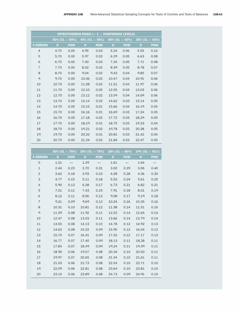
Fourth Pass


smi87468_app10B_10B1-10B67 10B-63 09/15/15 07:17 PM


50% (CL = 50%) 45% (CL = 55%) 40% (CL = 60%) 35% (CL = 65%)


4 4.70 0.00 4.95 0.03 5.24 0.06 5.55 0.10

5 5.70 0.00 5.97 0.02 6.29 0.05 6.63 0.08

6 6.70 0.00 7.00 0.03 7.34 0.05 7.71 0.08

7 7.70 0.00 8.02 0.02 8.39 0.05 8.78 0.07

8 8.70 0.00 9.04 0.02 9.43 0.04 9.85 0.07

9 9.70 0.00 10.06 0.02 10.47 0.04 10.91 0.06

10 10.70 0.00 11.08 0.02 11.51 0.04 11.97 0.06

11 11.70 0.00 12.10 0.02 12.55 0.04 13.03 0.06

12 12.70 0.00 13.12 0.02 13.59 0.04 14.09 0.06

13 13.70 0.00 14.14 0.02 14.62 0.03 15.14 0.05

14 14.70 0.00 15.15 0.01 15.66 0.04 16.19 0.05

15 15.70 0.00 16.16 0.01 16.69 0.03 17.24 0.05

16 16.70 0.00 17.18 0.02 17.72 0.03 18.29 0.05

17 17.70 0.00 18.19 0.01 18.75 0.03 19.33 0.04

18 18.70 0.00 19.21 0.02 19.78 0.03 20.38 0.05

19 19.70 0.00 20.22 0.01 20.81 0.03 21.42 0.04

20 20.70 0.00 21.24 0.02 21.84 0.03 22.47 0.05

30% (CL = 70%) 25% (CL = 75%) 20% (CL = 80%) 19% (CL = 81%)


0 1.21 — 1.39 — 1.61 — 1.66 —

1 2.44 0.23 2.70 0.31 3.00 0.39 3.06 0.40

2 3.62 0.18 3.93 0.23 4.28 0.28 4.36 0.30

3 4.77 0.15 5.11 0.18 5.52 0.24 5.61 0.25

4 5.90 0.13 6.28 0.17 6.73 0.21 6.82 0.21

5 7.01 0.11 7.43 0.15 7.91 0.18 8.01 0.19

6 8.12 0.11 8.56 0.13 9.08 0.17 9.19 0.18

7 9.21 0.09 9.69 0.13 10.24 0.16 10.35 0.16

8 10.31 0.10 10.81 0.12 11.38 0.14 11.51 0.16

9 11.39 0.08 11.92 0.11 12.52 0.14 12.65 0.14

10 12.47 0.08 13.03 0.11 13.66 0.14 13.79 0.14

11 13.55 0.08 14.13 0.10 14.78 0.12 14.92 0.13

12 14.63 0.08 15.22 0.09 15.90 0.12 16.04 0.12

13 15.70 0.07 16.31 0.09 17.02 0.12 17.17 0.13

14 16.77 0.07 17.40 0.09 18.13 0.11 18.28 0.11

15 17.84 0.07 18.49 0.09 19.24 0.11 19.39 0.11

16 18.90 0.06 19.57 0.08 20.34 0.10 20.50 0.11

17 19.97 0.07 20.65 0.08 21.44 0.10 21.61 0.11

18 21.03 0.06 21.73 0.08 22.54 0.10 22.71 0.10

19 22.09 0.06 22.81 0.08 23.64 0.10 23.81 0.10

20 23.15 0.06 23.89 0.08 24.73 0.09 24.91 0.10

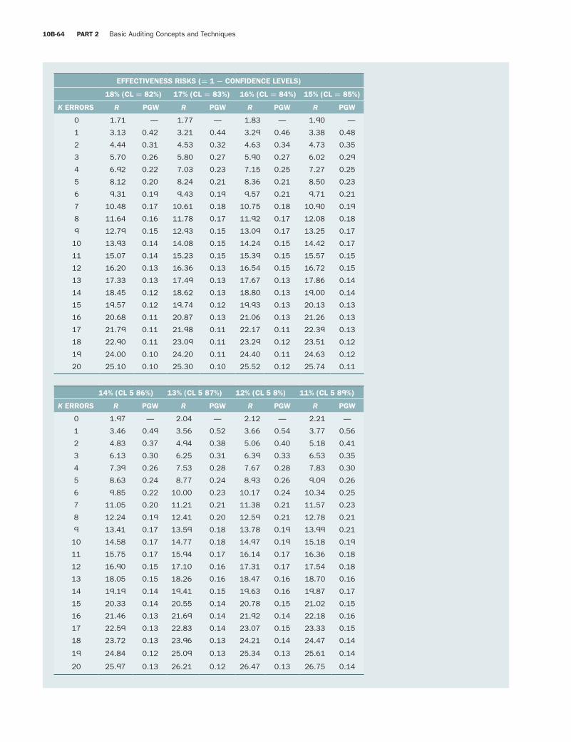
Fourth Pass


smi87468_app10B_10B1-10B67 10B-64 09/15/15 07:17 PM


18% (CL = 82%) 17% (CL = 83%) 16% (CL = 84%) 15% (CL = 85%)


0 1.71 — 1.77 — 1.83 — 1.90 —

1 3.13 0.42 3.21 0.44 3.29 0.46 3.38 0.48

2 4.44 0.31 4.53 0.32 4.63 0.34 4.73 0.35

3 5.70 0.26 5.80 0.27 5.90 0.27 6.02 0.29

4 6.92 0.22 7.03 0.23 7.15 0.25 7.27 0.25

5 8.12 0.20 8.24 0.21 8.36 0.21 8.50 0.23

6 9.31 0.19 9.43 0.19 9.57 0.21 9.71 0.21

7 10.48 0.17 10.61 0.18 10.75 0.18 10.90 0.19

8 11.64 0.16 11.78 0.17 11.92 0.17 12.08 0.18

9 12.79 0.15 12.93 0.15 13.09 0.17 13.25 0.17

10 13.93 0.14 14.08 0.15 14.24 0.15 14.42 0.17

11 15.07 0.14 15.23 0.15 15.39 0.15 15.57 0.15

12 16.20 0.13 16.36 0.13 16.54 0.15 16.72 0.15

13 17.33 0.13 17.49 0.13 17.67 0.13 17.86 0.14

14 18.45 0.12 18.62 0.13 18.80 0.13 19.00 0.14

15 19.57 0.12 19.74 0.12 19.93 0.13 20.13 0.13

16 20.68 0.11 20.87 0.13 21.06 0.13 21.26 0.13

17 21.79 0.11 21.98 0.11 22.17 0.11 22.39 0.13

18 22.90 0.11 23.09 0.11 23.29 0.12 23.51 0.12

19 24.00 0.10 24.20 0.11 24.40 0.11 24.63 0.12

20 25.10 0.10 25.30 0.10 25.52 0.12 25.74 0.11

14% (CL 5 86%) 13% (CL 5 87%) 12% (CL 5 8%) 11% (CL 5 89%)


0 1.97 — 2.04 — 2.12 — 2.21 —

1 3.46 0.49 3.56 0.52 3.66 0.54 3.77 0.56

2 4.83 0.37 4.94 0.38 5.06 0.40 5.18 0.41

3 6.13 0.30 6.25 0.31 6.39 0.33 6.53 0.35

4 7.39 0.26 7.53 0.28 7.67 0.28 7.83 0.30

5 8.63 0.24 8.77 0.24 8.93 0.26 9.09 0.26

6 9.85 0.22 10.00 0.23 10.17 0.24 10.34 0.25

7 11.05 0.20 11.21 0.21 11.38 0.21 11.57 0.23

8 12.24 0.19 12.41 0.20 12.59 0.21 12.78 0.21

9 13.41 0.17 13.59 0.18 13.78 0.19 13.99 0.21

10 14.58 0.17 14.77 0.18 14.97 0.19 15.18 0.19

11 15.75 0.17 15.94 0.17 16.14 0.17 16.36 0.18

12 16.90 0.15 17.10 0.16 17.31 0.17 17.54 0.18

13 18.05 0.15 18.26 0.16 18.47 0.16 18.70 0.16

14 19.19 0.14 19.41 0.15 19.63 0.16 19.87 0.17

15 20.33 0.14 20.55 0.14 20.78 0.15 21.02 0.15

16 21.46 0.13 21.69 0.14 21.92 0.14 22.18 0.16

17 22.59 0.13 22.83 0.14 23.07 0.15 23.33 0.15

18 23.72 0.13 23.96 0.13 24.21 0.14 24.47 0.14

19 24.84 0.12 25.09 0.13 25.34 0.13 25.61 0.14

20 25.97 0.13 26.21 0.12 26.47 0.13 26.75 0.14

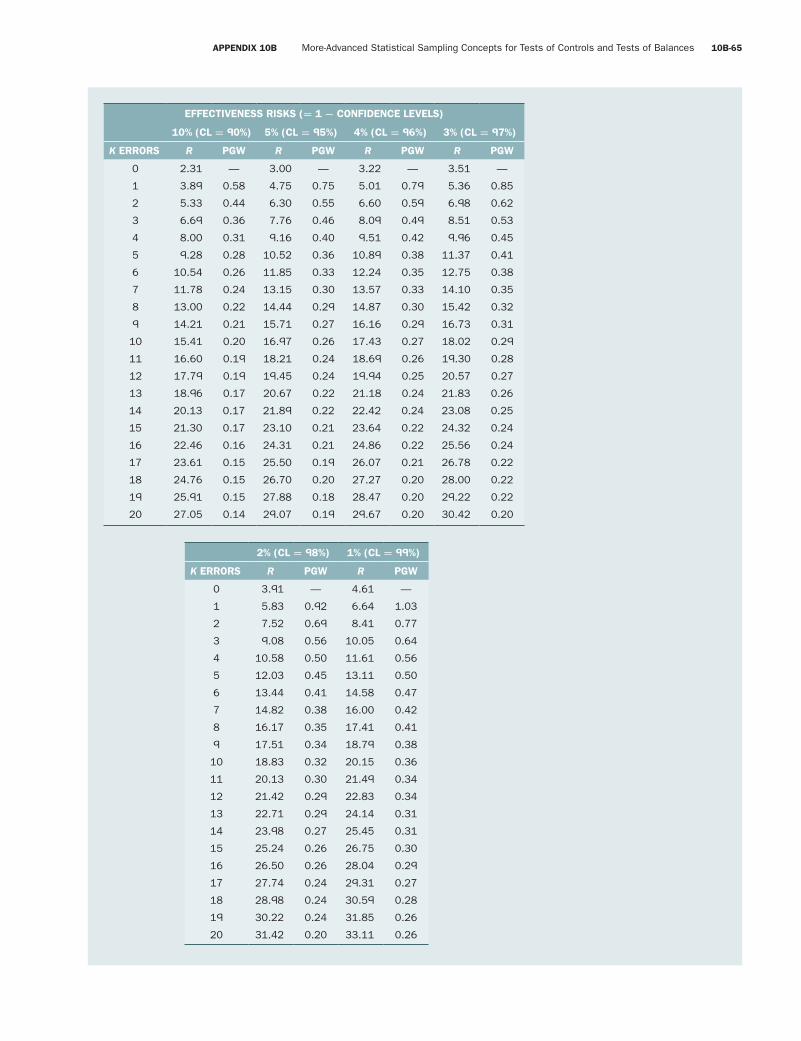
Fourth Pass


smi87468_app10B_10B1-10B67 10B-65 09/15/15 07:17 PM


10% (CL = 90%) 5% (CL = 95%) 4% (CL = 96%) 3% (CL = 97%)


0 2.31 — 3.00 — 3.22 — 3.51 —

1 3.89 0.58 4.75 0.75 5.01 0.79 5.36 0.85

2 5.33 0.44 6.30 0.55 6.60 0.59 6.98 0.62

3 6.69 0.36 7.76 0.46 8.09 0.49 8.51 0.53

4 8.00 0.31 9.16 0.40 9.51 0.42 9.96 0.45

5 9.28 0.28 10.52 0.36 10.89 0.38 11.37 0.41

6 10.54 0.26 11.85 0.33 12.24 0.35 12.75 0.38

7 11.78 0.24 13.15 0.30 13.57 0.33 14.10 0.35

8 13.00 0.22 14.44 0.29 14.87 0.30 15.42 0.32

9 14.21 0.21 15.71 0.27 16.16 0.29 16.73 0.31

10 15.41 0.20 16.97 0.26 17.43 0.27 18.02 0.29

11 16.60 0.19 18.21 0.24 18.69 0.26 19.30 0.28

12 17.79 0.19 19.45 0.24 19.94 0.25 20.57 0.27

13 18.96 0.17 20.67 0.22 21.18 0.24 21.83 0.26

14 20.13 0.17 21.89 0.22 22.42 0.24 23.08 0.25

15 21.30 0.17 23.10 0.21 23.64 0.22 24.32 0.24

16 22.46 0.16 24.31 0.21 24.86 0.22 25.56 0.24

17 23.61 0.15 25.50 0.19 26.07 0.21 26.78 0.22

18 24.76 0.15 26.70 0.20 27.27 0.20 28.00 0.22

19 25.91 0.15 27.88 0.18 28.47 0.20 29.22 0.22

20 27.05 0.14 29.07 0.19 29.67 0.20 30.42 0.20

2% (CL = 98%) 1% (CL = 99%)

K ERRORS R PGW R PGW

0 3.91 — 4.61 —

1 5.83 0.92 6.64 1.03

2 7.52 0.69 8.41 0.77

3 9.08 0.56 10.05 0.64

4 10.58 0.50 11.61 0.56

5 12.03 0.45 13.11 0.50

6 13.44 0.41 14.58 0.47

7 14.82 0.38 16.00 0.42

8 16.17 0.35 17.41 0.41

9 17.51 0.34 18.79 0.38

10 18.83 0.32 20.15 0.36

11 20.13 0.30 21.49 0.34

12 21.42 0.29 22.83 0.34

13 22.71 0.29 24.14 0.31

14 23.98 0.27 25.45 0.31

15 25.24 0.26 26.75 0.30

16 26.50 0.26 28.04 0.29

17 27.74 0.24 29.31 0.27

18 28.98 0.24 30.59 0.28

19 30.22 0.24 31.85 0.26

20 31.42 0.20 33.11 0.26

Fourth Pass


smi87468_app10B_10B1-10B67 10B-66 09/15/15 07:17 PM

Table of Random Digits

3294207410599814625165558

9541699859681552543751904

4233983828456736965493123

5904521409762109971627887

2669329094582191156353138

4905765114457380880321488

8749636701295508602709095

2062425762247365186778777

1481912827095741211671240

9918735641140316067766314

1925800301009361507605212

8642116096815189255467859

1640134775484402604289356

1939721562022182347220056

8329797983047566986930648

4011145040195066287787349

4932619200606951958420389

8168616383884943957653805

2041628701745796261593945

8741056992338445234206293

7564670423334268296822879

6417662415075707554008161

8275240807007288004501442

6360698086070795306975071

3701158850193222066521427

5734628968563252128294842

6951245297848190776826210

7568902921142950530357071

7613116919349699110990357

9683735424142168240312901

6745093209031914031208899

4451152133616476219191039

5042487327302966702367251

8284895897666679007328701

4197565171101018320503846

7166320376632037134494589

7847189242149554244618534

5774179337595924188022346

1359959293970353741554556

8439047481804304747217558

3214607740872200451373689

0087143345063924949414894

0935425716790280886005030

2274570020571230803819561

6580654005528724362456517

3928433922783550884501769

3373737329540139914571825

4251289911507749431655957

8641155876306668897498271

2375328379612052982802784

2969081031425749706966731

2609622058477739032740311

8136121487360276184288495

9309954613271742960418821

1763905851423961331860571

3828458653401121419254786

5947899949114699816726281

9040963505034767563101855

2199740409033287414130706

5619985551842382236966578

3006890729265703675732019

8280064938517908911765884

6969252403421225499858485

0953172865563247819264666

8185316829310932162634767

5933486542779249139997298

7092900396286220723592708

0354420363835430710401994

1851013010289127365253188

8954169645150596442578476

1355549608801928514907804

2116854738839647540962404

8220115360681421913828155

7569473776679573120003521

0280840914708963061636415

6598385190379831463978452

7437354278204874440692359

6669399054953504423681091

1309462944163715736056513

7418347351034268164488321

7302089098138959476197910

8797158147188757510935983

2903168841528095647403742

5178053625705947411176822

2737602059416493196612073

8105675223329352996959463

8615516783264307009384420

5548819272820969890115868

5059061994016058455099505

7451471090658462576911426

Source: The Rand Corporation, A Million Random Digits with 100,00 Normal Deviates (Glencoe: Free Press, 1955), p. 102.

Fourth Pass


smi87468_app10B_10B1-10B67 10B-67 09/15/15 07:17 PM

E N D N O T E S

1 Public accounting firms that use quantitative test of controls sampling policies have quantified probabilities underlying their categories, and they fall in the ranges indicated in Exhibit 10B–3.

2 A random start in a table may be obtained by poking a pencil at the table, or by checking the last four digits on your $10 bill to give row and column coordinates for a random start.

3 Most auditors will not allow the same sample item to appear twice in a selection—duplicate selections are counted only once. Strictly speaking, this amounts to sampling without replacement, and the hypergeometric probability distribution is appropriate instead of the binomial distribution. The binomial probabilities are exact only when each sample item is replaced after selection, thus giving it an equally likely chance of appearing in the sample more than once. For audit purposes, the practice of ignoring the distribution is acceptable because the difference is mathematically insignificant.

4 See D. A. Leslie, A. D. Teitlebaum, and R. J. Anderson, Dollar-Unit Sampling: A Practical Guide for Auditors (Toronto: Copp Clark Pitman, 1979).

5 There are other methods for calculating an MUS UEL. They are more complicated and require a computer.

6 The purpose of these calculations is to take into account both overstatement and understatement errors. It is not valid to (a) net the sample errors themselves and project the net error or (b) net the two total UELs to arrive at a net UEL. Actually, the calculations described in this chapter are the simplest of other more-complex calculations.

7 K. W. Stringer and J. R. Stewart, Statistical Techniques for Analytical Review (STAR) (New York: Deloitte, Haskins & Sells, 1985).

8 See Y. Chen and R. A. Leitch, “An analysis of the relative power characteristics of analytical procedures,” Auditing, A Journal of Practice and Theory, Fall 1999, pp. 35–69.

9 D. A. Leslie, Materiality, The Concept and Its Application to Auditing (Toronto: CICA, 1985), Ch. 8.

10 J. Tucker, “An early contribution of Kenneth W. Stringer: Development and dissemination of the audit risk model,” Accounting Horizons, June 1989, pp. 28–37.

more-advanced statistical sampling concepts for...

Documents