Morse TheoryGabor Pete

Trinity College, University of Cambridge, UK10 May 1999

Bolyai Institute, University of Szeged, Hungary20 July 2001

0

Contents

0. Introduction . . . . . . . . . . . . . . . . . . . . . . . . . . . . . . . . . . . . . . . . . . . . . . . . . . . . . . . . . . . . . . . . . . . . . . . . . . .10.1. The classical approach . . . . . . . . . . . . . . . . . . . . . . . . . . . . . . . . . . . . . . . . . . . . . . . . . . . . . . . . . . . . . . . . . . 20.2. First applications . . . . . . . . . . . . . . . . . . . . . . . . . . . . . . . . . . . . . . . . . . . . . . . . . . . . . . . . . . . . . . . . . . . . . . . 5

1. Preliminaries . . . . . . . . . . . . . . . . . . . . . . . . . . . . . . . . . . . . . . . . . . . . . . . . . . . . . . . . . . . . . . . . . . . . . . . . . . .91.1. Bundles on surfaces . . . . . . . . . . . . . . . . . . . . . . . . . . . . . . . . . . . . . . . . . . . . . . . . . . . . . . . . . . . . . . . . . . . . 91.2. Connexions and curvature . . . . . . . . . . . . . . . . . . . . . . . . . . . . . . . . . . . . . . . . . . . . . . . . . . . . . . . . . . . . . 121.3. Clifford bundles and Dirac complexes . . . . . . . . . . . . . . . . . . . . . . . . . . . . . . . . . . . . . . . . . . . . . . . . . . 161.4. The exterior bundle as a Dirac complex . . . . . . . . . . . . . . . . . . . . . . . . . . . . . . . . . . . . . . . . . . . . . . . 181.5. Analytic properties of the Dirac operator . . . . . . . . . . . . . . . . . . . . . . . . . . . . . . . . . . . . . . . . . . . . . .191.6. Hodge theory and the index of the Dirac operator . . . . . . . . . . . . . . . . . . . . . . . . . . . . . . . . . . . . . 211.7. The Atiyah-Bott-Lefschetz fixed point theorem . . . . . . . . . . . . . . . . . . . . . . . . . . . . . . . . . . . . . . . .221.8. The harmonic oscillator and quantum mechanics . . . . . . . . . . . . . . . . . . . . . . . . . . . . . . . . . . . . . . . 241.9. Supersymmetry theories . . . . . . . . . . . . . . . . . . . . . . . . . . . . . . . . . . . . . . . . . . . . . . . . . . . . . . . . . . . . . . 26

1.10. Around the Laplace operator . . . . . . . . . . . . . . . . . . . . . . . . . . . . . . . . . . . . . . . . . . . . . . . . . . . . . . . . . . 27

2. Supersymmetry and Morse theory . . . . . . . . . . . . . . . . . . . . . . . . . . . . . . . . . . . . . . . . . . . . . . . . . 29

3. Supersymmetry and Killing vector fields . . . . . . . . . . . . . . . . . . . . . . . . . . . . . . . . . . . . . . . . . . 33

4. Hamiltonian dynamical systems and Morse theory . . . . . . . . . . . . . . . . . . . . . . . . . . . . . . . . 364.1. Hamiltonian dynamical systems and symplectic geometry . . . . . . . . . . . . . . . . . . . . . . . . . . . . . . 364.2. The Morse theory of geodesics . . . . . . . . . . . . . . . . . . . . . . . . . . . . . . . . . . . . . . . . . . . . . . . . . . . . . . . . . 384.3. Volume growth and the complexity of the geodesic structure . . . . . . . . . . . . . . . . . . . . . . . . . . . 404.4. Morse theory on symplectic manifolds . . . . . . . . . . . . . . . . . . . . . . . . . . . . . . . . . . . . . . . . . . . . . . . . . .42

5. The Yang-Mills theory of connexions . . . . . . . . . . . . . . . . . . . . . . . . . . . . . . . . . . . . . . . . . . . . . . . 435.1. Characteristic classes and the Gauss-Bonnet-Chern theorem . . . . . . . . . . . . . . . . . . . . . . . . . . . 435.2. The YM functional and its critical points . . . . . . . . . . . . . . . . . . . . . . . . . . . . . . . . . . . . . . . . . . . . . . 455.3. Holomorphic line bundles and the Narasimhan-Seshadri theorem . . . . . . . . . . . . . . . . . . . . . . . 465.4. Some physics . . . . . . . . . . . . . . . . . . . . . . . . . . . . . . . . . . . . . . . . . . . . . . . . . . . . . . . . . . . . . . . . . . . . . . . . . . 47

6. Discrete Morse theory . . . . . . . . . . . . . . . . . . . . . . . . . . . . . . . . . . . . . . . . . . . . . . . . . . . . . . . . . . . . . . . .48

References . . . . . . . . . . . . . . . . . . . . . . . . . . . . . . . . . . . . . . . . . . . . . . . . . . . . . . . . . . . . . . . . . . . . . . . . . . . . . . . 50

1

0. Introduction

A first version of this essay was originally written in 1999 as one of my six Part III exams forthe degree Certificate of Advanced Study in Mathematics, at the University of Cambridge, UK.Now this is a slightly corrected and improved version, containing more details both on someintroductory and on some advanced topics. I would like to thank the help of Prof. GraemeSegal, who was my supervisor for this Part III essay topic, and Prof. Nandor Simanyi, whopatiently answers all my stupid questions concerning almost all parts of geometry. The summerschool Algebraic geometry in theoretical physics, organized by the Association of HungarianPhysicist Students (MAΦHE) in 2000, was a very nice and useful experience, too.

Morse theory is a method to determine the topology of a finite or infinite dimensional mani-fold (such as the space of paths or loops on a compact manifold) from the critical points of onlyone suitable function on the manifold. The theory has many far-reaching applications: Gauss-Bonnet theorem, Poincare-Hopf index theorem, the determination of the geodesic structure ofa manifold, Lefschetz singularity theory of hypersurfaces, Milnor’s exotic spheres, Bott’s peri-odicity theorem about the homotopy groups of the unitary and orthogonal groups, Yang-Millstheory on vector bundles, the planar n-body problem, geometry of Hamiltonian dynamical sys-tems, Floer homology, and has strong connections with the Atiyah-Bott-Lefschetz fixed pointand Atiyah-Singer index theorems.

The purpose of our essay is two-fold. The starting idea was to describe and explain E. Wit-ten’s supersymmetric approach to Morse theory. During writing this essay we found that thisexplanation should consist of not only a guide into tools used directly in this approach, butalso of an overview of connected geometrical notions and results. So we try to give an accountof a significant part of geometry from the point of view of Morse theory. We hope that thecommon roots and goals of the various mathematical theories described in this essay will helpthe Reader to gain a deeper insight into modern geometry.

The classical approach is beautifully written in J. Milnor’s book [M2] from 1963, containingsome of the older applications. In the first part of our Introduction we describe this originalproof of the basic result of the theory very briefly, just to give the Reader a general feeling aboutthe topic. The second part of the Introduction contains some well-known and/or conceptuallyeasier applications of Morse theory, such as Smale’s refinement of the theory, the Poincare-Hopfindex theorem, the Gauss-Bonnet theorem and Poincare duality.

In his 1982 paper [W1], Witten developed the whole theory with the help of some pertur-bated generalized Laplacian operators acting on the exterior bundle of differential forms on themanifold, using various ideas and techniques coming from supersymmetric quantum mechanics.Analyzing the asymptotic behaviour of these perturbated Laplacians he was able to prove notonly the strong Morse inequalities and the Poincare-Hopf index theorem, which are the mainresults of Morse theory, but also to develope a degenerate Morse and Poincare-Hopf theory, andto describe (conjecturally) the whole cohomology of the manifold through Morse theory, whichis a kind of finite-dimensional analogue of Floer homology. Since then this approach has beenapplied to serious problems in supersymmetry (SUSY) and also led to an asymptotic proof ofthe Atiyah-Singer index theorem, which has played a central role in the geometry of the pastfew decades.

First we overview the necessary background for Witten’s proof, including: connexions andcurvature in fibre bundles over differentiable and complex manifolds; the Dirac and Laplacianoperators of Clifford bundles; some PDE and functional analytic methods to prove the Hodgetheorem on the representation of cohomology by harmonic forms; the spectrum of the harmonicoscillator; the basics of quantum mechanics and supersymmetric theories. We also sketch theAtiyah-Bott-Lefschetz fixed point theorem together with some corollaries. As the key to thewhole theory is the intrinsic geometric meaning of the Laplacian and other elliptic differentialoperators on the manifold, we give a few different approaches to grap the geometry of a manifoldthrough the Laplacian, including some discrete probability theory, the Selberg trace formula,inverse spectral theory.

2

Next we give the proofs of Witten’s results mentioned above. As the original paper of himconcentrates on the mere ideas and not on the technicalities at all, there is a significant workin constructing the complete proofs in a clear way.

Among the many applications of Morse theory we focus on the description of the variationalcalculus of the geodesic flow and other Hamiltonian dynamical systems, and of the Yang-Millsfunctional defined on the space of connexions in a vector bundle. For instance, we prove theCartan-Hadamard theorem, the Gauss-Bonnet-Chern theorem, and give some account of theNarasimhan-Seshadri theory of curvature in vector bundles. We also overview certain othertopological consequencies of curvature, including some ergodic theory and geometric grouptheory. We end our essay with a short survey of discrete Morse theory, which is the analogueof the whole theory for simplicial complexes.

In understanding the background material for Witten’s approach my main help was thebook [R]. For a more elaborate treatise on differential geometry the Reader can always consultwith [DFN] or [KN]. For the Atiyah-Singer index theorem I can recommend [BGV] and [G]. Inparticular, [BGV] follows a description having deep similarities with the asymptotic methodsof [W1]. In writing this essay, the lecture notes [Se] and [Φ] were extremely useful. I also haveto recommend the beautiful short survey [B], which is a personal overview of the developmentof Morse theory. Finally, there is a very nice book [N], which I have encountered only veryrecently. This seems to be an excellent survey with almost the same purposes as I had in mind.

0.1. The classical approach

In this paper M usually denotes a compact n-dimensional smooth manifold. The ‘suitablefunction’ we mentioned at the beginning is meant to be a so-called Morse function. If we havethe manifold M , and a smooth function f : M −→ R, we call p ∈ M a critical point of fif in local coordinates around p we have ∂f/∂x1 = · · · = ∂f/∂xn = 0, i.e. if the differentialf∗ = Df has rank 0 (instead of 1). A critical point is non-degenerate if the Hessian matrixf∗∗ = (∂2f / ∂xi∂xj)n

i,j=1 is non-singular in p. In this case the number of its negative eigenvaluesis called the Morse index of the critical point. If the critical point is degenerate, then the numberof 0 eigenvalues is called the nullity of the critical point. A Morse function is a smooth functionf with only non-degenerate critical points (which are always isolated, as can be seen from thenext lemma). The following basic lemma gives a nice local description of a Morse function.

Lemma 0.1. (Morse lemma) If p ∈ M is a non-degenerate critical point of f then thereexist a neigbourhood U � p and local coordinates y1, . . . , yn such that yi(p) = 0 and f(q) =f(p) − y1(q)2 − · · · − yλ(q)2 + yλ+1(q)2 + · · · + yn(q)2 for q ∈ U , where λ is the index of f atp. �

Certainly, we can use our theory only if Morse functions do exist. One can find Morsefunctions among some kind of projection functions. The existence of a suitable point or directionfor such a projection can be proved by Sard’s theorem [DFN II, §10], [L], [MT], claiming thatthe set of critical values of a smooth function f : M −→ N between smooth manifolds is alwaysof measure 0 in N . Moreover, the set of Morse functions is dense in the space of all smoothfunctions on M in the C2-topology, which result is not significantly more difficult to prove.

The basic idea of classical Morse theory is that the homotopy (or, in better situations, eventhe homeomorphism or diffeomorphism) type of the submanifold Ma = {p ∈ M | f(p) ≤ a}changes only at the critical points of f . If there is no critical value in the interval [a, b], then thegradient flow of f provides a diffeomorphism between Ma and M b. At a critical value a, we cansuppose (after a small perturbation of f) that there is only one critical point p with f(p) = a.Now the key result is that we can get Ma+ε from Ma−ε by attaching a handle Bλ, a cell ofdimension of the index λ of f at the critical point f(p) = a. This handle Bλ can be constructedvia the description given by the Morse Lemma 0.1, and the attaching map is between ∂Bλ and∂Ma−ε. Then, using some technical results of Whitehead in homotopy theory, one can prove

3

the following theorem of crucial importance:

Theorem 0.2. If f is a Morse function on M such that Ma is compact for each a ∈ R thenM has the homotopy type of a cell complex with one λ-dimensional cell for each critical pointof index λ. �

Those results of Whitehead are needed to get not only a cell space, but a cell complex,which means that each cell is attached to cells of lower dimension. Instead of these homotopytheoretical methods there is a reformulation of the construction of the manifold by attachinghandles in the language of algebraic topology: one may use a Mayer-Vietoris type argument,e.g. the Excision theorem [DFN III, Thm. 5.9], [BT]:

If bk denotes the kth Betti number of M , i.e. the dimension of the cohomology groupHk(M ; R), and mk is the number of critical points of a Morse function f with index k, then

Theorem 0.3. (Morse inequalities) bk ≤ mk, moreover, we have

b0 ≤ m0

b1 − b0 ≤ m1 −m0

b2 − b1 + b0 ≤ m2 −m1 +m0

· · ·

χ(M) =n∑

k=0

(−1)kbk =n∑

k=0

(−1)kmk. �

The ‘official example’ of Morse theory is the height function on the torus embedded in R3 as adoughnut or bagel standing up vertically on a point of the great circle of the torus. This heightfunction has four critical points: one minimum (with index 0), two saddle points (with index 1)and one maximum (with index 2). And, in fact, the torus can be built up starting with a point,then attaching a segment to it, which form a circle together, then attaching another segment,resulting in a bouquet of two circles, then attaching a disk to this bouquet, resulting in the wholetorus. Another usual example is the complex projective space CP

n, with the Morse functionf(z0 : · · · : zn) =

∑i ci|zi|2, using the standard homogeneous coordinates, where the ci‘s are

different real numbers. Now f has exactly n+1 critical points (1 : 0 : · · · : 0), . . . , (0 : · · · : 0 : 1),with indices λi = 2|{j : cj < ci}|. Thus CP

n � B0 ∪ B2 · · · ∪ B2n, or, inductively, thecohomology of CP

n differs from that of CPn−1 by a single free generator in dimension 2n. A

basically similar method of computing the Betti numbers is to use the Weil conjectures (provedby Deligne, see [Si]), which involves counting the number of points of an algebraic variety overfinite fields. In particular, the inductive formula |FqPn| = |FqPn−1| + qn corresponds to thestratification of projective spaces we had earlier.

A closer look at the process of attaching the handles Bλ gives a decomposition of the manifoldinto handles in the smooth category:

Theorem 0.4. Every connected closed smooth manifold Mn is diffeomorphic to a union offinitely many handles Hn

λ = Bλ × Bn−λ, λ variable, where the handles Hnλ are in one-to-one

correspondence with the critical points of index λ. Conversely, given a decomposition of themanifold as a sum of handles, there exists a Morse function which gives rise to this given handledecomposition. �

Clearly, even if two manifolds have the same set of cells in their Morse decompositions,they do not have to be diffeomorphic, homeomorphic, or homotopic to each other — this stilldepends on the attaching maps between the handles!

A first interesting illustration of this problem is the following result, attributed to Reeb in[M2]: if f is an arbitrary smooth function having exactly 2 critical points on a compact n-manifold M , then M is homeomorphic to the n-sphere. For the case of non-degenarate criticalpoints this is a trivial consequence of Morse theory. If we allow for degenarate ones, as well,

4

then one can use the geodesic flow of f and the smooth Jordan curve (or sphere, in general)theorem for the level sets of f , which are diffeomorphic to an (n−1)-sphere. Then the manifoldcan be built up from two n-balls glued along an (n− 1)-sphere.

This result identifies Mn with Sn up to homeomorphism, but the diffeomorphism type ofMn depends on the smooth attaching map between the two standard (n − 1)-spheres at theboundaries. So the set of exotic differentiable n-spheres coincides with the set of essentiallydifferent orientation-preserving self-diffeomorphisms of the standard sphere Sn−1, i.e. with themapping class group Diff+(Sn−1). This group is usually non-trivial: the first exotic spheres inn = 7 dimension were found by Milnor [M1], and the number of them grows exponentially withn. Donaldson showed exotic differentiable structures e.g. on R4, see [DK]. On exotic spheressee also [M4] and [DFN III, Chp. 3].

Now we can already see how important it would be to describe the attaching maps viaMorse theory. A nice possibility could be to use the following transparent explanation on thedecomposition of the manifold into the handles Bλ. Consider the gradient flow φt

f : M −→Mof the Morse function f , corresponding to some Riemannian metric on M . The rest points ofthis flow are exactly the critical points of f , and the stable and unstable manifolds of a criticalpoint p,

W sp = {x ∈M : lim

t→∞φt(x) = p}, Wup = {x ∈M : lim

t→−∞φt(x) = p}

are λ(p) and (n − λ(p))-dimensional balls, where λ(p) is the Morse index at p. Therefore thestable manifolds give a decomposition of M into λ(p)-dimensional submanifolds, and we areroughly done. The problem is that this cell decomposition does not always represent a cellcomplex, and there could be problems with the attaching maps. S. Smale defined the gradient-like vector fields in [S1], which have two main properties: locally around every critical pointthere is a Riemannian structure in which the vector field is the gradient of a smooth function,and that the stable and unstable manifolds Wu

p and W sq intersect transversally in each of their

common points. He proved that for such a vector field we can find a so-called nice function(nowdays it is called a Morse-Smale function), whose gradient vector field coincides with thegiven vector field plus a constant around each critical point. These nice functions are those thathave only non-degenerate critical points, and have the self-indexing property: if f(p) = λ(p) forall critical points p. Secondly, he proved that every Morse function can be C1-approximatedby a nice function. Note that C2-approximation is impossible, since it would preserve Morseindices. As a corollary we can see that Morse-Smale functions always exist. An account ofMorse-Smale functions can be found in [DFN III, §17], too.

A careful inspection of the 2-dimensional case of Theorem 0.4, now already using a Morse-Smale function, easily gives the following classical result:

Theorem 0.5. (Classification of compact 2-manifolds) Every smooth, connected, compact2-manifold without boundary is homeomorphic (moreover, diffeomorphic) to a sphere with afinite number of handles and Mobius bands (crosscaps), attached in the usual way. In thepresence of at least one Mobius band, the sum of two Mobius bands is equivalent to one handle,and the manifold is orientable iff there are no Mobius bands at all. In such cases the numberof handles is called the genus g. The Euler characteristic is given by χ(M) = 2 − 2g. �

We have already mentioned that a manifold carrying a smooth function with only 2 criticalpoints is necessarily homeomorphic to a sphere. A natural problem is to minimize the numberof critical points on a given manifold M . First of all, when can the Morse inequalities mk ≥ bkbe sharp? Because of the second part of Theorem 0.4, if there is a cell decomposition of Mwith ck cells of dimension k, then we also have a Morse function with mk = ck, so the twominimalization problems are the same. I do not know about a manifold that forces a sharpMorse inequality, but Smale proved in [Sm3] that for n ≥ 5 dimensions the equalities mk = bkcan always be achieved. In fact, the problem ‘if an n-manifold M has the same Betti numbersas the n-sphere, does it follow that it can have a Morse function with exactly two critical points,and so it is homeomorphic to Sn?’ is known as the Poincare conjecture, which is solved for

5

n ≥ 5 by Smale [Sm2], for n = 4 by Freedman [DK], and is unsolved for n = 3. In [M3] wecan find a well-written Morse-theoretical proof of Smale’s h-cobordism theorem [Sm3], whichimplies the two theorems for n ≥ 5.

Theorem 0.6. (Smale’s h-cobordism theorem) If Wn+1 is a compact manifold-with-boundary with a disjoint union ∂W = V n

1 ∪ V n2 such that each Vi is 1-connected and is a

deformation retract of W , then W is diffeomorphic to Vi × [0, 1], and so V1 is diffeomorphic toV2. �

Here the basic idea is to pick a Morse-Smale function f on W , and, using the non-degeneracyconditions of Smale, to modify f such that the neighbouring critical points collapse (1st and2nd Cancellation Theorems), and we result in a Morse function f ′ without critical points atall. On cobordisms and smooth structures, besides [Sm2-3], see the above mentioned reference[DFN III, Chp. 3].

For the case of the tori Tn, now we desribe the solution to our problem. As Tn is a compactsymmetric space of Rn and also of itself as Lie-groups, its cohomology ring coincides with thering of its invariant differential forms [DFN III, Thm. 1.14], which is the free exterior algebraover the differentials dxi in our case. So bk(Tn) =

(nk

). On the other hand, if we construct the

torus by gluing the opposite faces of an n-cube, we get a cell decomposition with ck =(nk

), so

the optimum can be reached. An optimal Morse function can also be easily found: considerthe (π, . . . , π)- periodic function f(x1, . . . , xn) = cos2 x1 + · · ·+ cos2 xn on Rn. This is in fact asmooth function on Tn

π , having(nk

)critical points on the same level set of f for k = 0, 1, . . . , n.

The next question is what happens if we do not insist on Morse-functions, but allow forisolated degenerate critical points as well. The answer is given by the Lyusternik-Shnirelmantheory, see [DFN III, §19]. For a closed subset A ⊆ X of a Hausdorff space let us define itscategory catX(A) to be the least number k for which A can be written as a union of k closedsets Ai that are contractible in X . The two main results of the theory are that the number ofcritical points of a smooth function on M is always at least cat(M), and that cat(M) ≥ l + 1,where l = l(M) is the cohomological length of M . This length is the largest integer k such thatthere exist non-zero products α1 · · ·αk of k elements of positive degree in the comology ringH∗(M,Z). On cohomological multiplication see [DFN III, §7]. Calculating the exact value ofcat(M) is usually very difficult, but e.g. l(Tn) ≥ n is clear from our previous description of thering H∗(Tn,R). On the other hand, there is a smooth function on Tn having exactly n + 1critical points. Indeed, the Morse function f considered above can be perturbated so that the(nk

)critical points on each level set collapse, and we result in a function with n + 1 critical

points. Thus cat(Tn) = n+ 1, and this is the minimal number of isolated critical points.

One can continue the search for the topological consequences of few critical points. Forexample, for exactly three critical points (then the indices are 0, n/2, n, by Poincare duality,see later), we have manifolds which are like the real projective plane, see [M2, §4] and [EK].There can be 4 non-degenerate critical points on each of the 4-manifolds S4, S1 × S3, S2 × S2,and for manifolds with χ(M) = 0 these are the only homotopically different possibilities, see[Hu].

For critical points from a variational point of view (see Chapter 4) the Reader should try[MW].

0.2. First applications

Critical points and their indices are central objects in the theory of vector fields. So, first ofall, we briefly survey the corresponding degree theory. For more see [DFN II], [KH] and [MT].

The degree of a smooth map f : M −→ N between to n-dimensional oriented manifoldsis defined at a regular value y ∈ N as deg f(y) :=

∑f(x)=y sign detDf(x). This is in fact

independent of the choice of y, (moreover, invariant under homotopies on f), thus we have

6

defined deg f . The same notion can be expressed in two other languages: deg f :=∫

M f∗ω,where ω is a normalized volume form on N , that is a smooth differential n-form which is positiveon positively oriented frames,

∫Nω = 1, and f∗ω is its pullback. Also, deg f := fZ

∗n(1), wherefZ∗n : Hn(M,Z) −→ Hn(N,Z) is the induced homomorphism between homology groups.

Now we can define the index of a smooth map f : M −→ M at an isolated fixed point p.Locally we can think as f : Rn −→ Rn, and if V is an n-ball around p without more fixedpoints, then the smooth map

νf,V : ∂V −→ Sn−1, x �→ x− f(x)‖x− f(x)‖

is called the Gauss map. Now indpf := deg νf,V , which is independent of V . For a so-calledtransverse fixed point this index is easy to compute: if the spectrum of A = Df(p) does notcontain the value 1, then indpf = indpA = sign det(Id − A) — these two equalities are easyexercises.

The critical or singular points of a vector field X : M −→ TM are the rest points of itsflow φt

X : M −→ M , and the index of X at an isolated critical point p is the degree of thecorresponding Gauss map νX,V (x) = X(x)/‖X(x)‖, or equivalently, indpX := indpφ

tX , which

is of course independent of t ∈ (0, ε).If we consider a Morse function f : M −→ R, and its gradient flow φt

f corresponding tosome Riemannian metric, then the critical points of f will be the rest points of φt

f . Now indpφtf

is independent of the choice of the Riemannian metric and in locally Euclidean coordinatesaround a critical point p we have Dφt

f (p) = exp(tHp), where Hp is the Hessian f∗∗ at p. Thenon-degeneracy of p means 0 ∈ specHp, i.e. 1 ∈ spec exp(tHp), so p is a transverse fixed pointof φt

f . Thus indpφtf = signdet(Id − expHp) = (−1)λp , where λp is the Morse index.

Now the most important application of Morse theory in this direction is the following:

Theorem 0.7. (Poincare-Hopf index theorem) For an arbitrary vector field X : M −→TM , and its smooth flow φt

X : M −→M , we have

∑φt

X(p)=p

indpφtX = χ(M).

Proof. The sum of indices of the critical points of a vector field on a manifold is a topologicalinvariant, that is, it depends only on M , and not on X , see [DFN II, §15] or [MT]. (The mainreason is the homotopy invariance of the degree.) So it is enough to compute this sum for thegeodesic flow of a Morse function, which we have already done: it is

∑Df(p)=0(−1)λp . Now the

last equality in Theorem 0.3 gives the result. �

We will see a complete proof of the much more general degenerate Poincare-Hopf theoremin Chapter 3.

V. Arnold in [A, Appendix 9] writes that in 2 dimension the index of a critical point of agradient vector field can only be 1, 0,−1,−2,−3, . . . , while can be arbitrary in higher dimen-sions. Is it only by chance that these sets of possible indices coincide with the possible valuesof χ(Mn)/2, for orientable manifolds of the corresponding dimension?

It would be a natural wish to develop a Morse theory for fixed points of self-diffeomorphismsof a compact manifold, moreover, for smooth maps (e.g. embeddings) between different mani-folds, which would be a direct generalization of the standard Morse theory M −→ R. However,this is a far too hard problem in general. We saw that the self-diffeomorphisms of the standardsphere Sn−1 correspond to the exotic smooth structures on the n-sphere. The index theory ofvector fields can be directly applied to a self-diffeomorphism f only if the self-diffeomorphismis isotopic to the identity, i.e. we have a flow φt with φ0 = id and φ1 = f , since in this casewe have the vector field φ0. For example, a self-diffeomorphism f of S2 is of degree 1 or −1,and in the first case it is homotopic to id, in the second case this is true for −f . In the first

7

case the Poincare-Hopf theorem and an inspection of the indices at the critical points (comparethe result mentioned in the previous paragraph) give that we have at least two fixed points.It the second case we have at least two fixed points of −f . For a torus T2 we had at least 4non-degenerate critical points, but translation, for instance, has no fixed points at all. Thereis a deep theorem of Conley and Zehnder [CZ], resolving a special case of Arnold’s conjecture:a certain natural class of the so-called symplectomorphisms of T2n have at least 2n + 1 fixedpoints, and this number is at least 22n if all of them is non-degenerate. We will see more onthis topic in Section 4.4.

From our degree and Morse theories the Gauss-Bonnet theorem and its natural generaliza-tions can also be deduced [MT]:

Theorem 0.8. (Gauss-Bonnet theorem) For a compact oriented 2-manifold M we have

12π

∫M

K(p)Vol(p) = χ(M),

where K(p) is the Gaussian product curvature, which is the Jacobian of the Gauss map n :M −→ S2 ⊂ R3 arising at some isometric embedding M ↪→ R3.

Proof. First of all, note that the curvature K(p) is in fact independent of the embedding, thisis Gauss’s Theorema Egregium, see [DFN I, §30].

Now we can choose (by Sard’s theorem) a pair of regular antipodal points p± on S2: ifn(p) = p± then K(p) = 0. Now consider the projection f : M :−→ R ⊂ R3 onto the linedetermined by the points p±. This f has its critical points exactly at the points p ∈ Mfor which n(p) = p±. At any such point p, a neighbourhood of p can be parametrized by(u, v, f(u, v)), and in these local coordinates K(p) can be expressed via the Hessian f∗∗. Infact, the determinant of f∗∗ has the same sign as K(p), so the Morse index of f at p is even iffK(p) > 0. Thus by the usual Morse equality we have

χ(M) = |{p ∈M : n(p) = p±, K(p) > 0}| − |{p ∈M : n(p) = p±, K(p) < 0}|.

On the other hand, we have the same kind of expressions in the definition of deg n at theregular points p±, so we get χ(M) = degn(p+) + deg n(p−) = 2deg (n). Now we can considerthe pullback of the volume form on S2 by n: (n∗VolS2) (p) = K(p)VolM (p). Hence

∫M

K VolM =∫

M

n∗(VolS2) = (degn)∫

S2VolS2 = 4πdegn,

which, together with the previous result on deg n, gives the theorem. �

Instead of the Gaussian curvature in the tangent bundle we can consider arbitrary curvatureforms in real or complex vector bundles, as well. We will see this generalization in Section 5.2.

One of the most important computational tricks of any (co-)homology theory is the Poincareduality theorem, which has many different versions. In the smooth category [MT] it statesHk(M) � Hn−k

c (M)∗ for the deRham cohomology groups, where the ∗ stands for the dualvectorspace, c stands for the cohomology of forms with compact support, and M is not nec-essarily compact. Here the isomorphism is given by (ω1, ω2) �→

∫Mω1 ∧ ω2 for ω1 ∈ Hk(M),

ω2 ∈ Hn−kc (M). In the simplicial category [Ma], [DFN III], we have the Alexander-Poincare

theorem: if K is an orientable homology-n-manifold with a pair of subcomplexes L ≥ M ,and G is an Abelian group, then Hk(L,M ;G) � Hn−k(K −M,K − L;G); and the Lefschetztheorem for homology-n-manifolds-with-boundary: Hk(M,∂M ;G) � Hn−k(M ;G). The cell-homological Poincare theorem for compact manifolds follows easily from Morse theory [DFNIII, §18]. The basic idea is that changing a Morse function f on M to −f interchanges thestable and unstable manifolds, and thus we get a natural isomorphism between cells of comple-mentary dimensions. The proof in the simplical category uses dual polyhedra constructed via

8

the barycentic subdivision, and/or cap product, that is the simplicial counterpart of the smoothwedge product. We will see a proof for the smooth category in Section 1.6. For non-orientablemanifolds everything remains true over Z2.

Here are some immediate corollaries to Poincare duality. If H1(K; Z2) = 0, then K isorientable. No non-orientable homology-n-manifold can be embedded into Sn+1. If K ≥ Lare two homology-n-manifolds, then K = L. The cohomology ring H∗(CPn; Z) = Z[α]/αn+1,where degα = 2. The Borsuk-Ulam theorem. If M is a homology-n-manifold-with-boundary,then χ(∂M) is even. So, for instance, S2k and RP2k are not cobordant.

9

1. Preliminaries

In the following ten sections we give an account of the background material that we thinkto be necessary or at least useful in understanding the forthcoming more advanced topics inMorse theory. The most fortunate case would be if the Reader already knew almost everythingto be described here, and this chapter served only as a warm-up. Nevertheless, we shall try todescribe all the results in such details that seem to be enough to believe the validity of thesetheories. We will use the basics of differentiable manifolds, Riemannian geometry, algebraictopology, Lie groups and their Lie algebras without further warning — as we did it already inthe Introduction. For more information the Reader may turn to [DFN], [KN], [H1-2], [Se], [R],[BGV], [G].

1.1. Bundles on surfaces

A locally trivial fibre bundle with fibre F over a base space X is a continuous map π :Y −→ X such that every point x ∈ X has a neighbourhood U ⊆ X such that YU = π−1(U) ishomeomorphic to U × F by a map φU : YU −→ U × F taking each Yx = π−1(x) to {x} × F .Now Y is called the total space, X is the base space, π is the projection, and the Yx’s are thefibres. Sometimes the notation F −→ Y −→ X is used. A map ξ : X −→ Y with π ◦ ξ = idX

is called a section or cross-section.Analogously, we can define smooth bundles for smooth manifolds, and holomorphic bundles

for complex manifolds.Bundles usually have an additional structure, i.e. they are equipped with a structural group

G. This G is a group of transformations of F in the appropriate category, so it is a topologicalgroup acting on F from the left. All the transition maps φαβ = φβ ◦ φ−1

α : (Uα ∩ Uβ) × F −→Uα ∩ Uβ) × F are required to take the from (u, f) �→ (u, gαβ(u)f), with gαβ : Uα ∩ Uβ −→ G.

These transition maps gαβ are clearly continuous, gαα = idF , g−1αβ = gβα, and gαβgβγgγα =

idF . Conversely, if we are given such a family, we can construct a fibre bundle: Y := ∪(Uα ×F )/ ∼, where the equivalence relation is (uα, f) ∼ (uα, gαβ(uα)f). Two families {gαβ}, {gαβ}describe the same bundle if there are maps fα : Uα −→ G such that gαβ = fβgαβf

−1α .

The two most important examples are vector bundles and homogeneous spaces.

A rank k real vector bundle π : E −→ X is a bundle with fibre Rk and structural groupGL(k,R). For example, the tangent bundle TX of a smooth n-manifold is a rank n bundleover X . If the manifold has an atlas ϕα : Uα −→ Rn, then this atlas gives a natural localtrivialization φα : TUα −→ Uα × Rn, and we have the transition maps gαβ = D(ϕβ ◦ ϕ−1

α ).Differential k-forms are the smooth sections of the kth exterior bundle Λk(T ∗X), which alsohas a structural group GL(n,R). This space of sections is usually denoted by Ωk(X). Abundle is oriented if its structural group is G = GL+(n,R), the group of matrices with positivedeterminant. For example, the Mobius band of unbounded width is a non-orientable rank 1real vector bundle over the circle S1. We can also speak of complex vector bundles over realmanifolds, with structural group GL(k,C). On a real vector bundle over a paracompact basespace X , using partitions of unity, one can always construct an inner product 〈·, ·〉; this is acollection of inner products on each fibre Ex so that the map E −→ R, v �→ ‖v‖2 is continuous.Similarly, there is always a Hermitian inner product on complex vector bundles. Given alreadyan inner product on E, we can find local trivializations respecting this inner product, and thenthis bundle can be regarded as a bundle with structural group O(k) or U(k) — these are theEuclidean and Hermitian vector bundles.

Besides proving the results of the previous paragraph, here are some usual exercises for theReader. Show that a vector bundle is globally trivial, i.e. splits as a direct product, iff there isa nowhere-zero section of it. Show that the tangent bundle TS2 is not globally trivial. Showthat for any n-dimensional Lie group G, we have TG � G×Rn. It is a very deep result that theonly spheres with globally trivial tangent bundles are S0, S1, S3 and S7. The reason for them

10

to be globally trivial is that they are the unit spheres of the algebras R, C, H (the quaternions),and O (the Cayley octaves), respectively, and so they inherit something like a group structure.

With vector bundles we can do everything that is usual for single vector spaces: takingduals ∗, direct sums ⊕, tensor products ⊗, or form the bundle End(E) of fibrewise linearendomorphisms. It must also be clear for the Reader how to define the pulled-back bundle f∗Yover X ′ if we have a bundle Y over X , and a continuous map f : X ′ −→ X .

A complex vector bundle over a complex manifold is holomorphic iff the transition mapsgαβ : Uα ∩Uβ −→ GL(n,C) are holomorphic. If X is an n-dimensional complex manifold, thenits standard holomorphic tangent bundle TX is the space of C-linear maps from the germsof holomorphic functions to C. This is a holomorphic bundle TX = T 10X of complex rankn. But we can also consider the bundle T 01X of C-antilinear maps, which is a complex (butnot holomorphic) vector bundle of complex rank n. If we consider X as a 2n-dimensional realmanifold, then its complexified real tangent bundle TCX is a 2n-dimensional complex bundle,which splits as TCX = T 10X ⊕ T 01X . For the cotangent bundles we have T ∗

CX = Λ10(X) ⊕

Λ01(X), for the smooth sections we have Ω1C(X) = Ω10(X) ⊕ Ω01(X), and the complexified

exterior derivative dC : Ω0C(X) −→ Ω1

C(X) breaks up as dC = ∂ + ∂. A complex valued smooth

function f ∈ Ω0C(X) is holomorphic iff ∂f = 0 — in local coordinates this condition is the

well-known Cauchy-Riemann equality.Sometimes we do not have an honest complex manifold, but only an almost complex manifold,

which is an even-dimensional smooth manifold X with a smooth family of linear maps Jx ∈End(TxX) satisfying J2

x = −1. In this case a locally defined map f : U −→ C is said to beholomorphic if Df(x)(Jxv) = iDf(x)v for all v ∈ TxX . In this way we can also define thesplitting Ω1(X) = Ω10(X) ⊕ Ω01 as above. For two-dimensional surfaces it is true that everyalmost complex structure comes from a complex structure.

On R2, every linear map J2 = −1 is conjugated to the standard skew-symmetric matrix

J0 =(

0 −11 0

)

by an element g ∈ SL(2,R), and two such g1, g2 give the same J iff g−11 g2 ∈ SO(2), the

centralizer of J0. Thus the space of complex structures on R2 is isomorphic to SL(2,R)/SO(2),which is actually the upper half plane model of the hyperbolic plane. Therefore, a complexstructure on a 2-dimensional surface is given by a smooth map between two 2-dimensional realmanifolds. Since a diffeomorphism of a surface is specified by the same amount of data, it isunsurprising that the space of isomorphism classes of Riemann surfaces of a given genus is finitedimensional. In fact, if the genus is g, then this space is 6g − 6-dimensional.

The rank 1 complex vector bundles are called complex line bundles. The trivial line bundleOM := M × C, in the case of a compact complex M , has only constant holomorphic sections,by the maximum principle. In general, the complex vector space H0(M,E) of holomorphicsections of an arbitrary holomorphic vector bundle E over M is always finite dimensional —this is a special case of a finiteness theorem for sheaf cohomology. The canonical line bundleKM := Λn(T ∗M) = Λn0(M) is in fact a holomorphic line bundle if M is n-dimensional, andthe manifolds with KM = OM are of particular interest: they are the so-called Calabi-Yaumanifolds.

For the projective spaces CPn there is a holomorphic line bundle On(k) for every k ∈ Z:the total space is

((Cn+1 \ {0}) × C

)/C∗, where the action of λ ∈ C∗ is (z0, . . . , zn) × w �→

(λz0, . . . , λzn) × λkw. The bundle projection is the natural (z0, . . . , zn) × w �→ [z0 : · · · : zn].The sections of On(k) are clearly given by the holomorphic functions f : Cn+1 \ {0} −→ C

satisfying f(λz0, . . . , λzn) = λkf(z0, . . . , zn). For k ≥ 0 these are the homogeneous polyno-mials of degree k, and there is none for k < 0. Hence some simple combinatorics shows thatdimC H

0(CPn,On(k)) =? (an exercise for the Reader). The line bundle On(−1) has anothername: the tautological line bundle Hn. The reason for this name is that it can be desribed asHn = {([z], w) | [z] ∈ CPn, w ∈ Cn+1, w = λz, λ ∈ C}. The reason for the equality is that if one

11

picks local trivializations over the neighbourhoods Ui := {[z0 : · · · : zn] | zi = 0} ⊆ CPn, thenthe transition maps are readily seen to be gij = zj/zi in both cases. It is also easy to see thatH∗

n = On(1), OCPn = On(0), and On(k) ⊗On(l) = On(k + l), so we have a nice group of linebundles here.

To any fibre bundle with structural group G we can associate its principal bundle P with thesame structural group G, the same transition maps gαβ , but fibre G, with the natural left actionof the structural group G by left translations. Now, in any local trivialization PU � U × Gwe can consider the right action of G by right translations in each fibre. Since left and righttranslations of G commute, the result of this local right action is actually independent of thelocal trivialization chosen, and so defines a global right action on P . In general, a principalG-bundle P is a fibre bundle with structural group and fibre G. Clearly, P/G � X .

A homogeneous G-space is a smooth manifold X with a smooth transitive right action bya Lie group G. Because of transitivity, the stabilizers Gx of points x ∈ X are all isomorphicto the same Lie subgroup H , and the right quotient Lie-group G/H is naturally diffeomorphicto X . Here we have a fibre bundle with total space G, base space X , fibre H , and structuralgroup H , so this is a principal H-bundle. More generally, if H is a Lie group acting from theright without fixed points on a manifold Y , then (under some mild conditions) the orbit spaceX = Y/H inherits a smooth structure, and H −→ Y −→ X is a principal H-bundle.

Some important examples of homogeneous spaces: Zn −→ Rn −→ Tn, SO(n − 1) −→SO(n) −→ Sn−1, SU(n−1) −→ SU(n) −→ S2n−1, U(n−1) −→ SU(n) −→ CPn−1. A famousspecial case of the last example is the Hopf fibration S1 −→ S3 γ−→S2, where γ : S3 −→ S2 isthe following: S3 = {(z, w) ∈ C2 : |z|2 + |w|2 = 1} � SU(2), S2 � CP1, γ : (z, w) �→ −z/w.Check that the fibres over any two distinct points are two circles which are linked. We will seean interesting consequence of this fibration after Theorem 1.2.

The basic homotopy-theoretic fact about bundles is that if f0, f1 : X ′ −→ X are twohomotopic maps, and Y is a bundle over X , then f∗

0Y � f∗1Y . A simple corollary is that any

bundle on a contractible base is trivial. A more attractive application is the following:

Theorem 1.1. Isomorphism classes of bundles on a closed oriented surface (i.e. on a compact2-dimensional manifold) Σ with a connected structural groupG correspond precisely to elementsof π1(G).

Main idea of proof: The surface Σ can be covered by two contractible neighbourhoods, U1

and U2, intersecting in an annulus U . Now any bundle Y is locally trivial over U0 and U1, soY is given by a single transition map g01 : U −→ G. Using the homotopy-theoretical resultsabove, it is easy to see that the bundle Y depends exactly on the homotopy class of g01, i.e. ona class in π1(G). �

An important example is π1(GL(n,C)) � Z, where the isomorphism is given by assigningto a loop γ the winding number of det(γ) : S1 −→ C∗. For a complex vector bundle E onΣ the corresponding class C1(E) ∈ Z is called the first Chern class of E. Now it is alreadyless surprising that the complex line bundles On(k) form a group: a good exercise is to proveC1(O1(k)) = k.

The following generalization can be found in [DFN II, §24]: the isomorphism classes ofG-bundles over the sphere Sn are given by the homotopy group πn−1(G).

A second result about the nice behaviour of fibre bundles under homotopies is the (relative)homotopy lifting property, which has a corollary of crucial role in computing higher homotopygroups πk(X):

Theorem 1.2. (Homotopy exact sequence) Let π : Y −→ X be a fibre bundle with somearbitrary base points x ∈ X , y ∈ Y , π(y) = x, and with fibre F = π−1(x), with its inclusionmap ι : F −→ Y . Now there exists a homomorphism ∂ : πk(X,x) −→ πk−1(F, y) such that

12

the following sequence is exact:

· · · −→ πk+1(B) ∂−→πk(F ) ι∗−→πk(E)p∗−→πk(B) ∂−→πk−1(F ) −→ · · · �

Some homotopy groups of the spheres are easy to determine. By Sard’s theorem, a differen-tiable map Sk −→ Sn cannot be surjective for k < n, and from this πk(Sn) = 0 follows. Usingthe notion of degree defined in the Introduction, πn(Sn) = Z. However, the other cases are veryfar from trivial. Using Theorem 1.2, the striking corollary to the Hopf fibration we promised isπ3(S2) = Z. The higher homotopy groups of S2 are all known to be non-trivial, but they arenot completely described even conjecturally.

Using the examples of homogeneous spaces above, one can immediately see that πk(O(n)) =πk(O(n + 1)) for k ≤ n− 2, and πk(U(n)) = πk(U(n + 1)) for k ≤ 2n− 1. Thus, for example,π1(U(n)) = π1(U(1)) = Z and π1(O(n)) = π1(SO(n)) = Z2 for n ≥ 3. The second equality isbecause of the group isomorphism SO(3) � SU(2)/{±1}, which yields SO(3) � RP3. For thegroup isomorphism, consider SU(2) as the unit sphere of the quaternionic algebra H, and theaction of it by conjugation on the three dimensional real subspace of pure quaternions.

On the homotopy groups of the orthogonal and unitary groups a famous result is Bott’speriodicity theorem, a Morse theoretical proof of which can be found in [M]. This says thatπk(U(n)) = πk+2(U(n)) and πk(O(n)) = πk+8(O(n)) for all k ≥ 0 and all n (≥ 3 in theorthogonal case).

Note that GL(n,R) is homotopic to SO(n) and GL(n,C) is to U(n), so we have anotherproof of π1(GL(n,C)) � Z.

1.2. Connexions and curvature

On Rn there is a natural identification between any two tangent spaces TxRn and TyRn.However, on a general manifold we have to choose a connexion for transportation between dif-ferent tangent spaces. In this section we overview some different definitions of parallel transport,connexion, and the curvature of a connexion in fibre bundles F −→ Y

π−→X , with structuralgroup G.

Definition 1. A connexion is a rule assigning to each smooth path γ : [a, b] −→ X anisomorphism Tγ : Yγ(a) −→ Yγ(b) called the parallel transport along γ, with three properties:

(i) Transitivity: Tγ2 ◦ Tγ1 = Tγ2∗γ1 , if the composite path γ2 ∗ γ1 is well-defined and smooth.(ii) Strong parametrization independence: if θ : [a, b] −→ [c, d] is smooth with θ(a) = c,

θ(b) = d, but it is not necessarily bijective, then Tγ = Tγ◦θ.(iii) Tγ depends smoothly on γ, where the space of paths [a, b] −→ X is equipped with the

topology of uniform convergence of γ and all its derivatives.

Note that we have parallel transport for piecewise smooth paths, as well, because every pathcan be reparametrized to be stationary on some [a, a+ε] and on [b−ε, b], and so any compositionof two smooth paths will be smooth.

Connexion is a local object in the sense that if we have a connexion in YUα for each memberUα of an open covering of X , and they agree in each Uα ∩ Uβ, then we have a connexion inY . Also, a connexion in Y gives a connexion in the principal bundle P , and vice versa. For aprincipal G-bundle we can associate a vector bundle with fibre V and structural group G viaany linear representation ρ : G −→ GL(V ). These facts mean that it is enough to understandconnexions in principal bundles or in trivial vector bundles U × Rk, U ⊆ Rn.

So now we continue with a definition for principal bundles P/G = X .

Definition 2. Let V = ker(Dπ) ≤ TP be the sub-bundle of ‘vertical tangent vectors’ overP . A connexion is a G-equivariant splitting TpP = Hp ⊕ Vp, i.e. a choice of a complementarysub-bundle of ‘horizontal tangent vectors’. This splitting defines a ‘horizontal lift’ h(t, p) ∈ Hp

for any tangent vector t ∈ TxX with π(p) = x.

13

Given such a connexion, and a path γ from x to y in X , we can consider the tangent vectorfield of γ, and for any p ∈ Px we have a horizontal lift of this vector field, and so also ahorizontal lift of the path, which lifted path γ starts at p and ends at a point q ∈ Py . This mapPx � p �→ q ∈ Py is a parallel transport described in Definition 1, so we can really speak of aconnexion here.

As the vertical tangent space Vp is naturally identified with the tangent space of the fibre G,i.e. with the Lie algebra g of G, we can consider the splitting above as a projection αp : TpP −→Vp � g, where Hp = ker(αp). As G acts on P , it also acts on TP , and each u ∈ g induces aKilling vector field Ku : P −→ TP . The fact that G acts inside a fibre Px is equivalent toα(Ku) ≡ u. So a neat reformulation of the notion of a connexion is the following:

Definition 3. A g-valued 1-form α ∈ Ω1(P ; g) on P is a connexion 1-form if it is G-equivariant:α(v.g) = Ad(g−1)α(v) for all v ∈ TP and g ∈ G; and it represents a projection: α(Ku) ≡ u forall u ∈ g.

The three conditions for parallel transport in Definition 1 may appear to an inventive Readeras results of an infinitesimal description by a differential equation. So our next definition willbe such an infinitesimal one. It resembles the previous definition, but I do not know whetherthere is a nice formula describing the forthcoming 1-forms Aτ in terms of the global 1-form α.

Let τ : YU −→ U×F be a local trivialization, and Aτ ∈ Ω1(U, g) a Lie-algebra valued 1-formon U . Then we can locally define parallel transport along a curve γ : [a, b] −→ U by integratingthe first order ordinary differential equation

d

dtξ(t) +Aτ

(γ(t); γ(t)

)ξ(t) = 0 in Tξ(t)Y ;

if ξ(a) ∈ Yγ(a), then Tγξ(a) = ξ(b) ∈ Yγ(b). The three conditions of Definition 1 are fulfilled bystandard ODE theory.

Of course, we want our notion to be independent of the trivialization chosen. If we changetrivialization from τ to τ by a map g : U −→ G (now acting from the left), then for a section ξ(t)parallel along γ(t) we have ξ+Aτ (γ; γ)ξ = 0 in the old trivialization, and (gξ)+Aτ (γ; γ)(gξ) = 0in the new one. After substituting ξ = g−1η we find Aτ (γ; γ)η = gAτ (γ; γ)g−1η− gg−1η. Sinceγ and ξ were arbitrary, this means

Aτ = Ad(g−1)Aτ − dg · g−1,

which is the basic transition equality in gauge theory.

Definition 4. A connexion is a collection {Aτ} of 1-forms in Ω1(Uτ ; g) defined for all localtrivializations τ , and related by the transitions described in the equality above.

Finally, we describe connexions as a global way of differentiating sections in vector bundlesV −→ E −→ X . Suppose we have local trivializations over an open covering Uτ , and a globalsection ξ : X −→ E given locally by ξτ : Uτ −→ V . Let Aτ ∈ Ω1(Uα; End(V )) be a connexion,and define

dAτ ξτ := dξτ +Aτξτ ∈ Ω1(Uτ ;V ).

An easy calculation with transition maps shows that these local 1-forms dAτ ξτ fit together todefine a global 1-form dAξ ∈ Ω1(X ;E). So our last definition is the following:

Definition 5. A connexion A is given by a covariant derivative dA = ∇ : Ω0(X ;E) −→Ω1(X ;E) which is linear and satisfies the Leibniz rule dA(fξ) = fdAξ + dfξ for every sectionξ ∈ Ω0(X ;E) and function f ∈ Ω0(X ; K), where K = R or C, depending on the base field ofthe vector space V .

Note that in a holomorphic vector bundle E, dA acts on all smooth sections, and not onlyon the holomorphic ones.

14

For a tangent vector field v : X −→ TX the following notation is used sometimes: ∇ξ(v) =∇vξ, which suggests that we differentiate sections in the direction of a vector field. This alsomakes it useful to define ∇vf = v(f), i.e. dAf = df for f ∈ Ω0(M,K), for every connexionA. Moreover, we can define dA : Ωp(X ;E) −→ Ωp+1(X ;E) for all p by means of the formuladA(ξω) = dAξ · ω + ξdω for ξ ∈ Ω0(X ;E) and ω ∈ Ωp(X).

In general, a purely algebraic definition of connexion in an arbitrary module is the following.Let M be a module over a ring R; e.g. R = Ω0(X) has been our case so far. Then let Dbe the module of derivations of R, and Ω1

R = HomR(D;R). Now a connexion in M is amap M −→ M ⊗R Ω1

R of R-modules satisfying the Leibniz rule. At a cursory glance, theLie-derivative is also such a connexion, but it is of course not. For a tangent vector fieldw ∈ Ω0(X ;TX) we actually have [w, ·] ∈ Ω1(X ;TX), since [w, v]x depends not only on vx,but also on the whole v in a neighbourhood of x. One might speculate that the prize for theconnexion-freeness of the Lie-derivative is this non-tensorial property.

We also have a natural extension of covariant derivative for sections of End(E). If Θ ∈Ω0(X ; End(E)), and ξ ∈ Ω0(X ;E), then we would like to have dA(Θξ) = ΘdAξ + (dAΘ)ξ,which means dAΘ = dΘ + [A,Θ].

We can also see that any two connexions A and A in the same vector bundle E satisfydAξ − dAξ = aξ for some a ∈ Ω1(X ; End(E)). In other words, connexions in E form an affinespace for Ω1(X ; End(E)).

If our vector bundle E is equipped with some additional structure, e.g. with an Euclideanor Hermitian inner product, that one usually would like to use connexions compatible withthese structures. This means that the parallel transports Tγ are required to take values inthe structural group G, that is to be e.g. Euclidean or Hermitian isometries. It is easy toverify that for the covariant derivative this amounts to the compatibility condition d〈ξ, η〉 =〈dAξ, η〉 + 〈ξ, dAη〉. Using partitions of unity one can always construct such orthogonal orunitary connexions in a Euclidean or Hermitian vector bundle, respectively.

In the tangent bundle of a smooth manifold one is sometimes interested in torsion-free (orsymmetric) connexions. Clearly, ∇ itself is not tensorial, but its torsion tensor Tx(v, w) =∇wxv −∇vxw − [v, w]x depends only on the single tangent vectors vx and wx. Now ∇ is saidto be torsion-free if T (v, w) = 0 for all vector fields v, w. If ε ∈ Ω1(X ;TX) is the tautological1-form defined by ε(x; v) = v, then torsion-freeness is the property ∇Aε = 0. (Why?) On aRiemannian manifold there is exactly one symmetric connexion compatible with the Riemannianmetric; it is called the Levi-Civita connexion.

In a complex vector bundle E −→ X any connexion splits as dA = ∂A + ∂A, according tothe splitting Ω1(X ;E) = Ω10(X ;E) ⊕ Ω01(X ;E) of C- linear and C-antilinear maps. On theother hand, in a holomorphic bundle there is a canonical map ∂ : Ω0(X ;E) −→ Ω01(X ;E),defined without choosing a connexion. This map ξ �→ ∂ξ can be given locally in a holomorphictrivialization τ as ξτ �→ ∂ξτ , using the standard ∂ map of vector spaces, and these local sectionsfit together to define the global ∂ξ, because ∂ commutes with the action of transition maps,which is multiplication by holomorphic matrix-valued functions in this case. Thus we can makethe following definition: a connexion dA is compatible with the holomorphic structure of E if∂A = ∂.

Conversely, if X has complex dimension 1, then any connexion in a complex vector bundle Edefines a holomorphic structure, by claiming a locally defined section ξ holomorphic if ∂Aξ = 0,and then finding independent solutions ξ1, . . . , ξk to have holomorphic basis section for E. Thelocal solubility of ∂Aξ = 0 what holds only for dimC X = 1, and this is the same phenomenonthat we already encountered at the integrability of an almost-C-structure.

Now, if E is a holomorphic bundle with a Hermitian inner product, then there is a unique con-nexion dA which is both unitary and compatible with the holomorphic structure. For if the con-nexion 1-form A is given by A = P1(z1, . . . , zn)dz1+· · ·+Pn(z1, . . . , zn)dzn+Q1(z1, . . . , zn)dz1+· · · +Qn(z1, . . . , zn)dzn with respect to an orthonormal trivialization, then the Qi’s are deter-mined by the holomorphic structure, and then P = −Q∗ ensures unitarity. Alternatively, if weuse a holomorphic trivialization, the inner product is given by a Hermitian-matrix-valued func-

15

tion h, and the unitary condition dh = A∗h+ hA together with the holomorphic compatibilityimplies A = h−1∂h.

Summarizing these observations:

Theorem 1.3. For a complex Hermitian vector bundle E over a Riemann surface Σ (a complex1-dimensional manifold), the space A(E) of unitary connexions, which is an affine space forΩ1(Σ; End(E)), is isomorphic to the space C(E) of holomorphic structures. �

We also have a refinement of Theorem 1.1, which we do not prove here; a careful Readermight be able to do it alone.

Theorem 1.4. On a connected smooth manifold X , the isomorphism classes of princi-pal G-bundles with connexion are in bijection with the conjugacy classes of homomorphismsπ1(X) −→ G. This correspodence is given by parallel transport along closed curves in X . �

Using the extension dA : Ωp(X ;E) −→ Ωp+1(X ;E) as defined above, we can considerd2

A : Ωp(X ;E) −→ Ωp+2(X ;E), which, in contrast with d2 = 0, is an important object. It iscalled the curvature of the connexion, and in fact it is a tensor: FA = d2

A ∈ Ω2(X ; End(E)). Ifwe write dAτ = d+Aτ in a local trivialization, then

FAτ = dAτ +Aτ ∧Aτ .

The second (usually non-zero) term may look strange, but some contemplation should resultin the right definition. If we write Aτ =

∑iAidx

i in local smooth coordinates, then dAτ =∑i,j Ai,jdx

idxj and Aτ ∧Aτ =∑

i,j AiAjdxidxj , where Ai,j = ∂Ai/∂x

j.We can define curvature in a principal G-bundle, too. For a family {Aτ} of local g-valued

connexion 1-forms the appropriate formula is FAτ = dAτ + 1/2[A,A]. If we change localtrivialization from τ to τ by a transition map g, then FAτ = Ad(g−1)FAτ , which ensures theexistence of a global g-valued 2-form FA.

A fundamental result is that FA = 0 iff in every local trivialization there exists a basisξ1, . . . , ξn of smooth sections with dAξi = 0. For example, if X is simply connected, thenFA = 0 implies that E is globally trivial. In general, a connexion is called flat, if FA = 0.After the previous result it is not surprising that a connexion is flat iff the result of paralleltransport along γ depends only on the homotopy class of the curve. This can also be seen fromthe following description:

∂

∂uTu(p, q) =

∫ q

p

Tu(t, q)FA

(γu(t); γu(t),

∂γu(t)∂u

)Tu(p, t) dt,

where γu(t) is a smooth family of paths, and Tu(p, q) is parallel transport from γu(p) to γu(q)along γu.

Another definition of curvature which helps to visualize its meaning:

FA(x; v, w) = lims,t→0

1st

(Tγs,t − Id

),

where γs,t is the closed ‘rectangular’ path from x to x with side lenghts s, t, and side directionsv, w.

Let us mention the Bianchi identity: dAFA = 0.

Finally, let us have a look at the special case of a real oriented two-manifold Σ embeddedinto R3, with the Riemannian metric inherited from R3. In a coordinate patch of Σ we have anorthonormal tangent frame e1, e2, and the unit normal vector field is n = e1 × e2. Regardinge1, e2, n as maps Σ −→ R3, using the orthonormality of this system, we can write⎛

⎝ de1de2dn

⎞⎠ =

⎛⎝ 0 −α λ

α 0 μ−λ μ 0

⎞⎠

⎛⎝ e1e2n

⎞⎠ ,

16

for some α, λ, μ ∈ Ω1(Σ). Because of d2e1 = 0 we have λμ = dα.The area form VolS2 on the unit sphere in R3 is 1/2〈x, dx× dx〉, where x : R3 −→ R3 is the

identity map. So let us define the pulled back 2-form F = n∗(VolS2) = 1/2〈n, dn× dn〉 = λμ =dα = KVolΣ. This K, known as the Gaussian product curvature, see also Introduction 0.2,measures the rate at which n sweeps out area on S2, so it seems to be a right generalization ofthe curvature of curves. But what is the underlying connexion then?

In an orthonormal local trivialization {e1, e2} of TΣ, a connexion compatible with the innerproduct is a skew-symmetric matrix-valued 1-form, i.e. an element A ∈ Ω1(Σ)⊗ so(2,R). If wewrite out the torsion-freeness condition dAε = 0 in terms of the basis {e1, e2}, we find that theunique Levi-Civita connexion on Σ is

A =(

0 −αα 0

),

with the α ∈ Ω1(Σ) we had earlier! And what is the associated curvature FA = dA+A∧A? Sinceso(2,R) � R is a commutative Lie-algebra, the second term vanishes, and we find FA = dA, i.e.

FA =(

0 −dαdα 0

)=

(0 −KVolΣ

KVolΣ 0

).

Thus we have expressed the Gaussian curvature as the curvature of the Levi-Civita connexionin TΣ. Also note the naturality of the Levi-Civita connexion: ∇γ(t)ξ(t) is the 3-dimensionalderivative of ξ(t) along the curve γ(t), orthogonally projected to the tangent space Tγ(t)Σ. Sothe parallel transport of ξ(t) along γ(t) means that the 3-dimensional derivative of ξ(t) has notangential component at any time — the transportation is as economic as possible.

On Σ we can easily relate curvature to volume growth. In geodesic polar coordinates (r, θ)centered at some point of Σ, the metric is ds2 = dr2 + r2f2dθ2, where f is a smooth functionwith f(0, θ) = 1 and df(0, θ) = 0. Taking ε1 = dr and ε2 = rfdθ as an orthonormal basis for1-forms, we find

α = − ∂

∂r(rf)dθ and F = − 1

rf

∂2

∂r2(rf)VolΣ = KVolΣ,

where K is the Gaussian curvature at r = 0. This gives f(r, θ) = 1−1/3Kr2+O(r3). Knowingthat the metric on the unit sphere is given by dr2 + sin2 rdθ2, we can calculate now the area ofthe disc of radius r on Σ:

A(r) = πr2(

1 − 112Kr2 +O(r4)

).

1.3. Clifford bundles and Dirac complexes

In this section we make a rather abstract setup in order to define the ‘square root of theLaplacian’, the significance of which will become clear later. These Dirac operators on Cliffordbundles were intruduced the first time in [GrL].

If V is an n-dimensional real vectorspace with a symmetric bilinear form (·, ·), we can defineits Clifford algebra Cliff(V ) as a unital algebra A together with a structure map c : V −→ Asatisfying c(v)2 = −(v, v) · 1 ∈ A for every v ∈ V such that A is universal with respect to thisproperty; i.e. if A′ is another unital algebra with the same properties, with structure map c′,then there is a unique algebra homomorphism φ : A −→ A′ with c′ = φ ◦ c.

The uniqueness (up to a unique isomorphism) of such a universal algebra follows from theusual and trivial category theory argument. The existence can also be shown by the stan-dard method, factorizing the tensor algebra T (V ) by a suitable ideal. More explicitly, if V

17

has a basis e1, . . . , en, then A can be taken to be the linear span of the 2n possible prod-ucts c(e1)ε1 · · · c(en)εn , εi ∈ {0, 1}, with multiplication determined by c(v)c(w) + c(w)c(v) =−2(v, w). It is not difficult to see, that the dimension of Cliff(V ) is really 2n, and the structuremap is injective. So we will consider V as a subspace of Cliff(V ).

(Note that sometimes the structure map is determined by c(v)2 = (v, v) · 1 in the definition.Certainly, the only effect of this alteration is that multiplication by −1 or i =

√−1 occurs in

different places in the theory.)The simplest example is when the bilinear form is identically zero. Then the exterior algebra

Λ(V ) is the Clifford algebra, with multiplication ∧. Another important example is the Cliffordalgebra of R3 with the standard positive definite inner product, for which the notion wasoriginally introduced: it is isomorphic to H ⊕ H, where H is the quaternionic algebra. Clearly,Clifford algebras are Lie algebras with the usual commutator Lie bracket.

Clifford algebras naturaly arise in representation theory. Every representation of the Liegroups SL(n,C) and Sp(2n,C) can be found inside tensor powers of some standard representa-tions, but only half of the representations of SO(n,C) arise this way. In some sense the reasoncan be that the first two groups are simply connected, while π1(SO(n,C)) = π1(SO(n,R)) = Z2

for n ≥ 3. Clifford algebras help us to construct the spin groups, which are the double coveringsof these groups. For example,

S3 � Spin(3,R) � SU(2) −→ SO(3,R) � RP3.

In this essay we will not use the spin groups, but they are very important for the general theory.For more details on Clifford algebras see [R] and [HF].

Let us generalize our flat-space construction to the Riemannian manifold M . For any p ∈Mwe have the complexified Clifford algebra Cliff(TpM ⊗ C) � Cliff(TpM) ⊗ C. Now let S be avector bundle of Clifford modules, i.e. each fibre Sp is a module over (that is, a representationof) Cliff(TpM ⊗ C). To differentiate the smooth sections we need a connexion in S.

Let S be a complex vector bundle of Clifford modules over the Riemannian manifold M . Sis called a Clifford bundle if it is equipped with a Hermitian metric and a connexion compatiblewith it such that

(i) the hermitian metric is invariant under the Clifford action, that is, the action of a vectorv ∈ TpM by c(v) ≡ v on Sp is skew-adjoint: (vs1, s2) + (s1, vs2) = 0;

(ii) the connexion in S is compatible with the Levi-Civita connexion onM in the sense that forany two vector fields X,Y and section s ∈ C∞(S), we have ∇X(Y s) = (∇XY )s+Y∇Xs.

The Dirac operator D of a Clifford bundle S is the first order differential operator on C∞(S)defined by the composition

C∞(S) −→ C∞(T ∗M ⊗ S) −→ C∞(TM ⊗ S) −→ C∞(S),

where the first arrow is given by the connexion s �→ ∇...s, the second by the duality comingfrom the metric, and the third by the Clifford action. In terms of a local orthonormal basis ei

of sections of TM , one can writeDs =

∑i

ei∇is.

In the simplest case, when M is the flat vector space V , we have Ds =∑

i ei(∂is), and asimple computation gives D2s = −

∑i ∂

2i s, which is the Euclidean Laplacian. In the general

case the generalized Riemannian curvature of the connexion, the End(S)-valued 2-form R = R∇

R(X,Y )s = ∇X∇Y s−∇Y ∇Xs−∇[X,Y ]s

also appears. We can choose the local orthonormal tangent base ei s.t. [ei, ej ] = 0; in this basethe coefficients of R will be Rij = ∇i∇j−∇j∇i, and we haveD2s = −

∑i ∇2

i s+∑

i<j eiejRijs.

18

Clearly, the Laplace operator on functions on a Riemannian manifold can be written locallyas the sum of second partial derivations along geodesic coordinates, that is, as the image of theordinary Laplace on the tangent space under the exponential map.

If ∇∗ : C∞(T ∗M ⊗ S) −→ C∞(S) is the adjoint of ∇, then some computation shows thatthe previous equation can be written as the Weitzenbock formula, see [R, (2.6)],

D2s = ∇∗∇s+ Ks,

where K ∈ End(C∞(S)) is the curvature operator of S, defined by∑

i<j eiejRij . A similarcomputation shows the important result that D is self-adjoint. The operator ∇∗∇ is positive,K is self-adjoint, so the Weitzenbock formula easily gives the following

Theorem 1.5. (Bochner) If the least eigenvalue of K at each point of the compact M isstrictly positive, then there are no nonzero solutions of the equation D2s = 0. �

In the next section we will see that in the case of the exterior bundle our curvature operator isa generalization of the Ricci curvature operator, which is the (1, 1)-tensor field given by raisingone index of the Ricci curvature tensor K(X,Y ) = Tr(Z �→ R(X,Z)Y ), using the Riemannianmetric gij . We will see an application to Bochner’s theorem in Section 4.3.

We say that a Clifford bundle S on a compact oriented manifold is a Dirac complex if it isa direct sum S = ⊕k

j=0Sj of vector bundles with Hermitian metrics and compatible connex-ions, together with a sequence of differential operators dj : C∞(Sj) −→ C∞(Sj+1) satisfyingdj+1dj = 0, and the Dirac operator of the Clifford bundle is D = d + d∗, where d = ⊕k

j=0dj .Certainly, we also can define the Z2-grading, as above.

The main example of a Dirac complex will be the deRham complex on the exterior bundle. Afurther very important example is the Dolbeault complex on an (almost) complex manifold, see[R, (2.20)], [KN], and first of all, [GH]. Using the spin groups mentioned in the previous sectionone can introduce the spin manifolds and spin complexes. These are also Clifford bundles, andthe Atiyah-Singer index theorem for spin manifolds gives strong results for each of the usualDirac complexes. In our paper some kind of perturbated deRham complexes will play a centralrole, to be discussed in Chapters 2 and 3.

1.4. The exterior bundle as a Dirac complex

The most important example of a Clifford bundle is the exterior bundle of M . As a vectorbundle, S := ΛT ∗M⊗C is naturally isomorphic to Cliff(TM⊗C); the basis element e1∧· · ·∧ek

(the ei’s are orthonormal) of the exterior algebra corresponds to the basis element e1 · · · ek ofthe Clifford algebra. (This is not an isomorphism of algebras, since Cliff(V ) � Λ(V ) only in thecase of the zero bilinear form.) So S is a natural module over Cliff(TM ⊗ C), thus is a bundleof Clifford modules. Moreover, equipped with a natural metric and connexion it is a Cliffordbundle indeed. We describe it now in more details.

On an n-dimensional orientable compact Riemannian manifoldM there is exactly one n-formVol such that Volx(e1, . . . , en) = 1 for every orthonormal basis TxM . This is called the volumeform, and equals

√det(gij) dx1 ∧ · · · ∧ dxn, where g = gij is the Riemannian metric. Now we

can define the Hodge ∗ operation on the exterior bundle by

∗ : Ωr(M ;TM) −→ Ωn−r(M ;TM), (∗ω)(v1, . . . , vn−r)Vol = ω ∧ v1 ∧ · · · ∧ vn−r,

where v is the dual 1-form to the vector field v, w.r.t. the metric g, i.e. v(w) = (v, w)g for everyvector field w. We can extend g to a metric on arbitrary r-forms α, β locally at any point: if gij

is the inverse matrix of gij , then define (dxi, dxj) = gij , and (dxi1 ∧· · ·∧dxik , dxj1 ∧· · ·∧dxjk ) =det

((dxir , dxjs)

)k

r,s=1. Then we have a global inner product defined by

∫M

(α, β)Vol. Now

(α, β)Vol = β ∧ ∗α = α ∧ ∗β,

19

and ∗∗ = (−1)r(n−1) on ΛrT ∗M , see [R, Chp. 2] and [L, Chp. X and XIII].A vector field v defines two important operations on differential forms, independently of

the Riemannian metric. The interior multiplication or contraction i(v) : Ωr −→ Ωr−1 isdefined by (i(v)ω)x(v2, . . . , vr) = ω(v(x), v2, . . . , vr) for any r-form ω. Then we have ∗i(v)∗ω =(−1)nr+n+1v∧ω, and the operator i(v) is the adjoint of the exterior multiplication v∧, w.r.t. theglobal metric of forms. Sometimes the following notation is used: v�ω = (−1)n−1i(v)ω. Clearly,contraction is the unique antiderivation such that i(v)ω = ω(v) for 1-forms.

Secondly, we have the Lie-derivative Lv : Ωr −→ Ωr, the unique derivation which commuteswith d : Ωr −→ Ωr+1, the usual differential operator of forms, and extends the derivation offunctions alnog vector fields. Moreover, the Lie-derivative can be defined for any tensor field:it has to be the extension of the Lie-bracket of vector fields, as well: Lvw = [v, w] = vw − wv.A very improtant local description can be given by the flow αt generated by v:

Lvω =d

dtα∗

tω

∣∣∣∣t=0

.

Interior multiplication and Lie derivative are related by Cartan’s formula

di(v) + i(v)d = Lv,

which also expresses the homotopy invariance of deRham cohmology. For the computations see[L, Chp. V] or [DFN I].

Using Stoke’s theorem it turns out that the operator d∗ : Ωr −→ Ωr−1 defined by d∗ =(−1)rn+n+1 ∗ d∗ is the adjoint of d. For example, in Rn, dω =

∑i dx

i ∧ (∂ω/∂xi) and d∗ω =∑i i(∂/∂x

i)(∂ω/∂xi). With some additional formal calculations [R, Chp. 2] we can summarizeour description in the following result:

Theorem 1.6. The bundle S = ΛT ∗M ⊗ C is a Clifford bundle with Clifford action c(v)ω =v ∧ω+ v�ω, and Dirac operator D = d+ d∗. The Laplacian is D2 = dd∗ + d∗d. The restrictionof the curvature operator K to 1-forms is equal to the Ricci curvature operator. �

The exterior bundle splits as a direct sum of the even dimensional forms Λ+T ∗M and odddimensional forms Λ−T ∗M . We can introduce a Z2-grading: there is an involution ι with the+1 and −1-eigenspaces Λ+T ∗M and Λ−T ∗M , and

(Λ(−1)ν

T ∗M)∧

(Λ(−1)μ

T ∗M)⊆ Λ(−1)ν+μ

T ∗M.

Moreover, we have ιD +Dι = 0. Then the graded D splits as D+ ⊕D−, and D+ and D− arethe adjoints of each other.

1.5. Analytic properties of the Dirac operator

Now we will explain the main analytic properties of the Dirac operator on a Dirac complex.Our standard reference will be [R].

Let us define the Sobolev space W k(M) obtained by completing C∞(M) in the Sobolevk-norm

‖f‖k =∑|α|≤k

‖Dαf‖L2,

where α stands for multiindices (α1, . . . , αn), and Dα is the partial derivative (∂αi / ∂xαi

i )i. If Vis a vector bundle overM , we can define similarly the Sobolev spaceW k(V ) ofW k sections of V .The most important facts about these spaces are the Sobolev embedding theorem and Rellich’stheorem, see [R, Chp. 3]. The first one is that for p > n/2, the space W k+p is continuouslyincluded in Ck. The second one states that if k < l, then the inclusion operator W l −→ W k

20

is compact. Clearly, multiplication by a C∞ function acts as a bounded operator on each W k,and linear differential operators of order l act boundedly from W k to W k−l.

Since the Dirac operator D is a first order opearator, we have ‖Ds‖0 ≤ C‖s‖1 with someconstant C, for any s ∈ C∞(S) section. Some kind of converse is also true, which is the mainanalytic property of D; see [R, (3.15)]:

Lemma 1.7. (Elliptic estimate) For any k > 0 there is a constant Ck s.t., for any s ∈ C∞(S),

‖s‖k+1 ≤ Ck(‖s‖k + ‖Ds‖k). �

D is an unbounded operator on the Hilbert space H = L2(S), defined on C∞(S). Its graph isthe subspace of H⊕H defined as G = {(x;Dx) |x ∈ dom(D)}. It is easy to see that the closureG is also a graph, so defines an extended unbounded operator D. By the elliptic estimate itsdomain is exactly the Sobolev space W 1(S). Moreover, if for x, y ∈ L2(S) we have Dx = yweakly, i.e. (x,Ds) = (y, s) for all s ∈ C∞(S), then x ∈ W 1(S) and Dx = y. More generally, ifx, y ∈W k(S), (k ≥ 1), and Dx = y, then x ∈ W k+1(S). From now on we can consider D as abounded operator from W 1(S) to L2(S).

Theorem 1.8. The Hilbert-space H = L2(S) has a direct sum decomposition into countablymany orthogonal subspaces Hλ, where each Hλ is a finite dimensional space of smooth sections,an eigenspace for D with eigenvalue λ. The eigenvalues λ form a discrete subset of R.

Main idea of the proof. Using standard Hilbert space arguments we can construct a compactbounded operator Q : H −→ W 2(S) satisfying 1 = (1 +D

2)Q on H . The boundedness and

compactness of Q are due to Rellich’s theorem and the elliptic estimate on D. Now we can usethe standard knowledge of the spectrum of the compactQ, and translate this for the spectrum ofD. To show that the eigenvectors are smooth, one can use the results of the previous paragraphand the Sobolev embedding theorem. For details see [R, (3.25)]. �

If f is a bounded function on the spectrum σ(D), we can define a bounded operator f(D)on L2(S): the operator which acts as multiplication by f(λ) on each Hλ. One can easily provethe following observation:

Lemma 1.9. The map f �→ f(D) is a unital ∗-ring homomorphism from B(σ(D)) to B(H)(the spaces of bounded functions and operators, respectively). If D commutes with an operatorA, so does every f(D). Moreover, every f(D) maps C∞(S) to C∞(S). �

The spectrum of the ordinary Laplacian on a compact Riemannian manifold contains a largeamount of important geometrical data. First of all, it determines the dimension, the volumeand the total scalar curvature. For the number of eigenvalues not larger than λ the followingestimate holds, see [R, (7.3)]:

N(λ) ∼ 1(4π)n/2Γ(n

2 + 1)Vol(M)λn/2.

There was a long-standing question whether there exist isospectral manifolds which are notisometric. The answer is affirmative; for a nice introductory survey see [Br]. For other signs ofthe geometric significance of the Laplacian see Section 1.10.

As we will see in the next section, the finite-dimensional null-space of the Dirac operator D,which coincides with the null-space of D2 (the subspace H of the so-called harmonic sections),also has a crucial geometrical meaning, that is, it completely represents the cohomology ofthe Dirac complex on the manifold. This already explains the importance of the heat operatore−tD2

, t > 0, acting on L2(S) as defined by Lemma 1.9, which connects the identity operator(for t = 0) with the projection L2(S) −→ H (for t = ∞). This operator naturally appears inthe heat equation

∂st

∂t+D2st = 0;

21

in fact, for an initial state s0 ∈ C∞(S) we have the unique C∞(S) solution st = e−tD2s0. The

analytical properties we have discussed so far assert that this heat operator is a smoothingoperator, see [R (5.7)], that is, there exists a smooth heat kernel kt(m1,m2) on M ×M , t > 0,with values kt(m1,m2) ∈ Hom(Sm2 , Sm1), such that

e−tD2s(m1) =

∫M

kt(m1,m2)s(m2)Vol(m2).

A smoothing operator on M is of trace-class, which we do not define here, but it is worth notingthat if the bounded operator A has the smoothing kernel k(m1,m2), then

Tr(A) =∫

M

k(m,m)Vol(m),

and this trace coincides with the sum of the eigenvalues for self-adjoint operators.The asymptotic properties of this heat kernel play a key role in the theory of the Atiyah-

Singer index theorem. We will see some applications (without real proofs) in Section 1.7.

1.6. Hodge theory and the index of the Dirac operator

A bounded operator A : B1 −→ B2 between Banach spaces is called Fredholm if ker(A)is finite dimensional in B1 and im(A) is closed in B2 and of finite codimension. For such anoperator we can define its index by

ind(A) = dim ker(A) − codim im(A).

Clearly, if both Bi are finite dimensional, then ind(A) = dim(B1) − dim(B2), which is ratherstable under perturbations of A. In general Banach spaces we can allow for perturbations bycompact operators, for instance.

Lemma 1.10. The Dirac operator D is a Fredholm operator from W 1(S) to L2(S). Moreexactly, im(D) is the orthogonal complement of ker(D) in L2(S).

Proof. By Theorem 1.8, ker(D) is finite dimensional. From the self-adjointness of D it isobvious that im(D) ⊆ ker(D)⊥. On the other hand, let f be a function on the spectrum σ(D)with f(0) = 0 and f(λ) = λ−1. Then for x ∈ ker(D)⊥ we have Df(D)x = x, see Theorem 1.8and Lemma 1.9. As usually, Df(D)x ∈ L2(S) implies f(D)x ∈W 1(S), so x ∈ im(D). �

We can define the cohomology Hj(S, d) of smooth sections of a Dirac complex as for any chaincomplex. For the deRham complex on the exterior bundle it is of course the usual cohomology ofthe manifold, this is deRham’s theorem, see [BT] or [DFN III]. This cohomology is independenton the metric, but we have the Laplacian Δ = dd∗ + d∗d = D2, and the spaces of smoothharmonic sections satisfying Δs = Ds = 0. The central idea of Hodge theory is that we canchoose a canonical harmonic representative for each cohomology class.

In the basic case we are given a (real or complex) graded Hilbert space A = ⊕np=0A

p with alinear map d = dp : Ap −→ Ap+1 satisfying d2 = 0. Let Hp(A) = ker dp/imdp−1. Define theLaplacian Δ = dd∗ + d∗d, where d∗ is the adjoint of d with respect to the Hilbert space innerproduct, and define the harmonic subspace H = kerΔ. If the following two Hodge conditions

(i) kerΔ is finite dimensional(ii) H⊥ = ΔA

hold, then elementary Hilbert space manipulations give the Hodge decomposition [L, Chp. X.5]:

A = H⊕ dA⊕ d∗A

andH =

n⊕

p=0Hp with Hp � Hp(A),

22

where Hp = H ∩Ap.In the case of a Dirac complex we already know that the Hodge conditions are satisfied, by

Lemma 1.10. So, being a little bit careful about the difference between C∞(S) and L2(S), weget immediately the following theorems of crucial importance:

Theorem 1.11. (Hodge theorem) Each cohomology class has a unique harmonic repre-sentative, i.e. Hj � Hj(S, d) as vector spaces. �

The trivial example is the harmonic functions on M , which are constant on each connectedcomponent [KN II, Note 14], and the group H0(M) with dimension being equal to the numberof connected components. In [R, (4.2)] there is a more direct proof of the Hodge Theorem,constructing a chain equivalence between the Dirac complex and its subcomplex of harmonicsections with 0 differential. The chain homotopy operator (see [BT] or [MT]) is H = d∗G,where G = g(D) is the Green’s operator defined by the function g(0) = 0, g(λ) = λ−2 on thespectrum σ(D).

One can think of these harmonic representatives from a geometric point of view. If C ⊆C∞(Sj) is a cohomology class, then it is an affine subspace of L2(S) with α− β ∈ dC∞(Sj−1)for all α, β ∈ C. Therefore we expect a norm-minimizing element α to be perpendicular todC∞(Sj−1), which translates to say that d∗α = 0. Since dα = 0, this is equivalent to D2α = 0.Unfortunately, the existence of this norm-minimizing element in a general Hilbert space is notnecessary, so this was not a proof for the Hodge theorem.

Corollary 1.12. The cohomology of a Dirac complex is finite dimensional. �

Corollary 1.13. (Poincare duality) If M is a compact connected oriented n-manifold,then Hk(M) � Hn−k(M). �

From Lemma 1.10 we know that ind(D) = 0, but the index of D+, which is also a Fredholmoperator, already contains some important geometrical data.

Corollary 1.14. The index of D+ equals to the Euler characteristic of the Dirac complex(S, d). �

1.7. The Atiyah-Bott-Lefschetz fixed-point theorem

The Lefschetz number L(φ) of a smooth self-map of Mn, with isolated non-degenerate fixedpoint only, can be defined in three different ways:

L(φ) =∑

φ(m)=m

signdet(I −Dmφ) =n∑

k=0

(−1)kTr(φ∗k) = Δ(φ) ◦ Δ,

where Δ ⊆ M ×M is the diagonal, Δ(φ) = (x, φ(x))x∈M , and ◦ is the intersection index ofsubmanifolds in M ×M , see our Introduction 0.2 and [DFN II]. The usual Lefshetz theorem isthe equivalence of these definitions. Now we are going to consider a generalization.

If φ : M −→ M is a smooth map, then it induces an endomorphism φ∗ : C∞(S) −→C∞(φ∗S). Assuming we have a bundle map ζ : φ∗S −→ S, for example, the natural ζ = Λ∗D∗φin the case of the deRham complex, where D∗φ is the dual to the derivative Dφ, then we havethe composite map F = ζφ∗ : C∞(S) −→ C∞(S). (I hope there will be no confusion fromthe two meanings of D, one for the derivative, one for the Dirac operator.) Now, if F satisfiesFd = dF , then we call the pair (ζ, φ) a geometric endomorphism of the Dirac complex, and wecan define the Lefschetz number

L(ζ, φ) =n∑

q=0

(−1)qTr(F ∗ on Hq(S, d)).

23

The Lefschetz number of the identity map is clearly the Euler characterictic of the Dirac com-plex.

Now it is not difficult to prove that if Pq denotes the orthogonal projection L2(Sq) −→ Hq,then Tr(F ∗ on Hq(S)) = Tr(FPq), and the smoothing kernel of e−tΔq tends to the smoothingkernel of Pq in the C∞ topology, where Δq is the restriction of D2 to C∞(S). Thus we haveTr(FPq) = limt→∞ Tr(Fe−tΔq), and a corresponding formula for the Lefschetz number. Buta ‘supersymmetric cancellation of eigenspaces’ yields the same result for every t > 0; we willmeet a similar phenomenon in Chapter 3:

Lemma 1.15.∑n

q=0(−1)qTr(Fe−tΔq) = L(ζ, φ), independently of t.

Sketch of the proof. After differentiating our equation by t, we seee that we have to prove∑nq=0(−1)qTr(F (dd∗ + d∗d)e−tΔq) = 0. Using dF = Fd and Δqd = dΔq+1, the terms in the

sum will cancel in pairs, resulting in 0; the only problem is that d is an unbounded operator,so we can have problems with computing trace, but this is only some kind of technicality; fordetails see [R, (8.6)]. �

This formula immediately gives ind(D+) = Trs(e−tD2), cf. Corollary 1.14, where Trs(A) =

Tr(ιA) is the super-trace of the graded operator A, ι is the grading operator.Looking at the diagonal of the heat kernel, Lemma 1.15 gives a generalized Lefschetz fixed-

point theorem: if φ has no fixed points, then L(ζ, φ) = 0. A detailed analysis of the heat kernelgives the following strong result, see [AB1] and [R, (8.11)]:

Theorem 1.16. (Atiyah – Bott) If (ζ, φ) is a geometric endomorphism having only simplefixed points, that is, det(1 − Tmφ) = 0 (implying that m is an isolated fixed point), then

L(ζ, φ) =∑

φ(m)=m

n∑q=0

(−1)qTr(ζq(m))| det(1 −Dmφ)| . �

For the ordinary deRham complex we cannot expect more than the original Lefschetz indextheorem. Using the fact that Tr(ΛqT ) is nothing else but the qth elementary symmetric poly-nomial of the eigenvalues of T , one can see that

∑q(−1)qTr(ΛqT ) = det(1 − T ). On the other

hand, for an isolated simple fixed point we have indmφ = indmDmφ = signdet(1 −Dmφ), aswe saw in the Introduction 0.2. Thus we have

L(φ) =∑

φ(m)=m

sign det(1 −Dmφ) =∑

φ(m)=m

indmφ.

Usual applications are the Brouwer fixed point theorem and the Poincare-Hopf index theorem.For a flow φt : M −→M each φt is homotopy equivalent to the identity φ0, thus we have

∑φt(m)=m

indxφt = L(Id) = χ(M).

If we have a Morse function f on M , then we can apply this for the gradient flow of f , andhave

∑k Mk = χ(M), as in the strong Morse inequalities Theorem 0.3.

We will see a degenerate Poincare-Hopf theorem in Chapter 3.

More interesting corollaries to the Atiyah-Bott Theorem 1.16 can be achieved if we considerDirac complexes other than the ordinary deRham complex, such as the Dolbeault complex, spinmanifolds, and representations of a Lie groups. Lots of beautiful applications can be found in[AB1], and we will also give some of them at the end of Chapter 3. A typical example for thecomplex analytic case is the following:

Let X be a connected compact complex manifold with H0,q(X) = 0 for q > 0. Then anyholomorphic map f : X −→ X has a fixed point. In particular, if X is a complex projective

24

space, then any holomorphic automorphism has a fixed point. Sometimes we can guaranteelots of fixed points, see the end of Chapter 3, again.

1.8. The harmonic oscillator and quantum mechanincs

The harmonic oscillator is the unbounded operator

H = − d2

dx2+ a2x2 (a > 0)

on L2(R). The aim of this section is to determine its spectrum and give some introduction tothe very important role of this operator in physics.

There are the corresponding annihilation (or lowering) operator A = ax + ddx , the creation

(or raising) operator A∗ = ax− ddx . Elementary computations give

AA∗ = H + a, A∗A = H − a

[A,A∗] = 2a, [H,A] = −2aA, [H,A∗] = 2aA∗.

The ground state of H is the function ψ0 ∈ L2(R) satisfying the differential equation Aψ0 = 0and ‖ψ0‖ = 1. Then it is clearly an eigenfunction Hψ0 = aψ0, and it is easy to calculate itexplicitly:

ψ0(x) = a1/2π−1/4 e−ax2/2.

For k ≥ 1 we can define the excited states of H inductively by

ψk = (2ka)−1/2A∗ψk−1.

They are also eigenfunctions Hψk = (2k + 1)aψk, with ‖ψk‖ = 1. The names ‘raising’ and‘lowering’ operators come from the fact that if Hψ = λψ, then H(A∗ψ) = (λ + 2a)A∗ψ andH(Aψ) = (λ − 2a)Aψ. (Note that this does not mean that we could produce an eigenfunctionfrom ψ0 with smaller eigenvalue than a, since Aψ0 = 0.)

Now it is clear by induction that ψk(x) = hkxe−ax2/2, where hk is a polynomial of degree k.

So these ψk’s span the space P = {p(x)e−ax2/2 | p is a polynomial}, and it is not too difficultto see that this is a dense subspace of L2(R). Thus we have proved the following result; for thedetails see [R Chp. 10]:

Theorem 1.17. The space L2(R) has a complete orthogonal decomposition into 1-dimensionaleigenspaces of the harmonic oscillator with discrete spectrum {(2k + 1)a | k = 0, 1, . . . }. �

From the respect of the the general theory the heat equation of the harmonic oscillator,

∂st

∂t+Hst = 0,

is also very important.

The harmonic oscillator is an extremely important example for quantum mechanics andthe supersymmetry theories of mathematical physics. The 1-dimensional classical harmonicoscillator is the dynamical system governed by the Hamiltonian

H(q, p) =1

2m(p2 +m2ω2q2),

where q(t) is the coordinate for the space, p(t) is the momentum, m is a constant for the massand ω is a constant for the frequency. Time evolution is given by the Hamiltonian equations

q =∂H

∂p, p = −∂H

∂q,

25

or, in terms of the Poisson bracket for functions F (q, p) and G(q, p),

{F,G} =∂F

∂q

∂G

∂p− ∂F

∂p

∂G

∂q,

they can be written asq = {q,H}, p = {p,H}.

The functions of the canonical variables p and q form an infinite- dimensional Lie algebra withthis Poisson-bracket, and time evolution is always given by F = {f,H}. Poisson bracket canbe more generally defined in case of symplectic manifolds, which arise naturally in the theoryof Hamiltonian dynamical systems; see also Chapter 4 and [KH].

In quantum mechanics the states of a system are not single coordinates (q, p), but complexwave functions ψ(q) with real density functions |ψ(q)|2. The momentum wave function ψ(p) isjust the Fourier transform of ψ(q), and |ψ(q)|2 is again a probability density. For any classicalfunction f(q, p), we would like to introduce a Hermitian operator F acting on the complexHilbert space of the states, such that to the classical function i�{f, g} always the operator[F,G] has to correspond, where � = h/2π, h is Planck’s constant. In particular, the classicalcanonical variables p and q satisfy the commutation relations {q, q} = {p, p} = 0, {p, q} = 1,so we would like to produce quantum mechanical operators P and Q with the commutationrelations [Q,Q] = [P, P ] = 0, [Q,P ] = i�I, this is called quantization. One realization of suchan operator Lie algebra is given by the operators

Qψ(q) = qψ(q), Pψ(q) = −i�∂ψ(q)∂q

.

Setting A = 1/√

2(P − iQ) and A∗ = 1/√

2(P + iQ), we have the so-called bosonic commu-tation relations [A,A] = [A∗, A∗] = 0 and [A,A∗] = I, which (apart from constants) is the Liealgebra generated by A,A∗, I, we had before; this is the three-dimensional Heisenberg algebra,with Lie group consisting of matrices of the form

⎛⎝ 1 a b

0 1 c0 0 1

⎞⎠ , a, b, c ∈ R,

called the Heisenberg group.For a dynamical system with Hamiltonian H , which is expected to be Hermitian, time

translation is given by the operator eiHt. In particular, if ψ(q) is an eigenfunction of H witheigenvalue λ, then ψt = eiHtψ will differ from ψ only in phase, ψt(q) = ψ(q)eiλt. Thus|ψt(q)|2 ≡ |ψ(q)|2, which means that ψ(q) is an equilibrium state for the system.

From the relation [Q,P ] = i�I one can easily deduce the Heisenberg uncertainity relation,stating that (ΔP )(ΔQ) ≥ �/2 on every state ψ, where (ΔP )2 is the variation according to theprobability density |ψ|2. Clearly, the physical relevance of the above construction by quantiza-tion is known by experimental results. For an introduction to quantum mechanics see [Li], and[SW] for the Heisenberg algebra.

Raising and lowering operators also appears in the representations of every Lie algebra.Consider, for example, the most important semisimple Lie algebra, sl2 = sl(2,C), having anatural complex basis

E =(

0 10 0

)F =

(0 01 0

)H =

(1 00 −1

)

with commutation relations

[E,F ] = H, [H,E] = 2E, [H,F ] = −2F.

26

If V is a finite dimensional representation, i.e. a left sl2-module, and v ∈ V is a Hv = λveigenvector (a so-called weight vector with weight λ), then HEv = (λ + 2)Ev and HFv =(λ− 2)Fv, so E increases, F decreases the weight by 2. The main result is the following

Theorem 1.18. The finite dimensional irreducible representations of sl2 are classified by their‘highest weight’, a positive integer d. The irreducible representation Vd has dimension d + 1and has a unique ‘highest weight vector’ (up to scalar multiple) v ∈ Vd satisfying Hv = dv andEv = 0. If v0 = v and vj = j−1Fvj−1 for j = 1, . . . , d, then these vj ’s form a basis of Vd withHvj = (d− 2j)vj . �

For the structure and representations of Lie algebras see [FH] and [H2].

In general, we are speaking about a system of bosonic annihilation and creation operators ai

and a∗i , if they satisfy the commutation relations

[bi, bj] = [b∗i , b∗j ] = 0, [bi, b∗j ] = δijI,

and fermionic annihilation and creation operators fi, f∗i , if they satisfy the anticommutation

relations{fi, fj} = {f∗

i , f∗j } = 0, {fi, f

∗j } = δijI,

with the brackets [A,B] = AB −BA and {A,B} = AB +BA.For example, the Lie algebra sp(2k,C) can be represented by bosonic operators, the Lie

algebra so(2k,C) is by fermionic operators. In our paper the crucial example is the exteriorbundle Λ(T ∗M) with the fermionic creation operators a∗i = dxi∧ (exterior multiplication) andannihilation operators ai = i(∂/∂xi) (interior multiplication), as introduced in Section 1.4. Onecan see immediately that they really satisfy the anticommutation relations prescribed above.

1.9. Supersymmetry theories

In fact, the Z2-grading introduced at the end of Section 1.4 is the key connection to su-persymmetry [W1]. By definition, a supersymmetry theory is a Hilbert space K = K+ ⊕ K−

decomposed into the spaces of bosonic and fermionic states, together with Hermitian ‘symme-try operators’ Qi, i = 1, . . . , N , mapping K+ into K− and vica versa. If (−1)F is the involutionwhich distinguishes the bosonic and fermionic subspaces, then this supersymmetry conditionreads as

(−1)FQi +Qi(−1)F = 0.

Secondly, we have a Hamiltonian operatorH which generates time translations, e.g. a differentialoperator governing a smooth dynamical system. The supersymmetry operators should commutewith it,

QiH −HQi = 0.

In the simplest form of supersymmetric quantum mechanics we have the further conditionspecifying the algebraic structure:

Q2i = H and QiQj +QjQi = 0 (for i = j).

If one wants the structure fit to the relativistic quantum field theory (now only with onespace and one time dimension), then we also need a momentum operator P , with the modifiedconditions

Q21 = H + P, Q2

2 = H − P, QiQj +QjQi = 0.

Now it follows that

[Qi, H ] = [Qi, P ] = 0, [H, (−1)F ] = [P, (−1)F ] = 0

27

and

H =12(Q2

1 +Q22).

The central question in a supersymmetry theory is the existence of a state |Ω〉 ∈ K annihilatedby all the supersymetry operators, Qi|Ω〉 = 0. For such a state we have P |Ω〉 = H |Ω〉 = 0, sothis state has zero energy, it is a vacuum state. (Clearly, for any state in K we have H |Ω〉 ≥ 0.)Supersymmetry basically means the existence of a vacuum state; in this case fermions andbosons have equal mass. If there is a minimal enery state, but it has strictly positive energy,then supersymmetry is ‘spontaneously broken’, fermions and bosons are not of equal mass,despite the underlying supersymmetry structure. In physics it is not clear at the momentwhether supersymmetry does play a role in nature or not.

For a vacuum state it is enough to look in the subspace K0 consisting of states annihilatedby P , and within this subspace our system looks like the simplest supersymmetry theory. Thatis, Q2

i = H for any i, and a state annihilated by one Qi is annihilated by all of them. So we arelooking for a zero eigenstate of one supersymmetry operator Q in K0. We have a decompositionQ = Q+⊕Q− according to the decomposition K = K+⊕K−, where Q+ and Q− are the adjointsof each other. Now it is worth considering the index indQ+ = dim kerQ+ − dim kerQ− =Tr(−1)F , since a nonzero index implies a zero eigenvalue of Q.

The reason for calling the subspaces K± as bosonic and fermionic subspaces is that in a su-persymmetry theory they are usually the subspaces generated by excited states created from thevacuum state by some bosonic and fermionic creation operators, respectively. In our geometricalexample one can think of the symmetric and exterior algebras S(V ) and Λ(V ) as the subspacesof bosonic and fermionic states of the tensor algebra T (V ), satisfying canonical commutationand anticommutation relations, respectively, see the end of Section 1.8; S(V ) is a commutativealgebra with multiplication α · β = S(α⊗ β), while Λ(V ) = ⊕n

i=0ΛnV is a graded commutative

algebra with α ∧ β = Λ(α⊗ β). Graded commutativity means α ∧ β = (−1)degα degββ ∧ α. Ageneral Clifford algebra can also be decomposed into bosonic and fermionic subalgebras, by thecanonical involution ι(x1 · · ·xk) = (−1)k(x1 · · ·xk) for xl ∈ c(V ).

1.10. Around the Laplace operator

This section is still to be written. At the moment we can give only a brief indication of thedesired contents.

In Sections 1.6 and 1.7 we have already seen how important can be the Laplacian. Anotherkind of geometric significance is revealed by the fact that the only differential operators invariantunder the isometries of a Riemannian manifold are more or less always the polynomials of theLaplacian, see [H1, Chp. X] and [Ha].

Let X be a Riemannian manifold with a given (usually discrete) group Γ of isometries.Now Γ also acts on function spaces over X , e.g. on L2(X,R), and we can speak of Γ-invariantfunctions an operators on X . The Selberg trace formula [Ha] relates the Γ-invariant eigenvaluesand eigenfunctions of invariant differential and integral operators, such as the Laplacian, to thegeometry of the qutient space X/Γ. This is a generalization of the Poisson summation formula.It can be viewed as the statement that two isospectral tori are isometric. For arbitrary manifoldsit is not true, though we have seen in Section 1.5 that the spectrum contains a lot of geometricdata. The Sunada trace formula gives a nice group-theoretic characterization of isospectral butnon-isometric manifolds. See [Br], which is a very nice survey on the subject of inverse spectralgeometry.

There is a discrete Laplacian for finite and infinite graphs and groups, which is basically thesame as the Markov operator of simple random walks on these graphs. This operator acts onthe L2-space of the graph, and the spectrum of it is closely related to the geometry of the graph,such as expanding properties, amenability, and geometric properties of random processes on the

28

graphs. If our graph is a lattice in a Riemannian manifold, then the geometric properties ofthe continuous and discrete Laplacians are the same. For example, the representation theoryof Lie groups has led to the construction of expanders. There is also a discrete potential theoryon infinite graphs, and the probabilistic boundary of the random walks, according to which wewould like to solve Dirichlet etc. problems, often has a geometric meaning, such as the Gromovboundary of hyperbolic groups. On these topics see [Lu] and [Wo].

29

2. Supersymmetry and Morse theory

In this chapter we will prove the weak and strong Morse inequalities of Theorem 0.3, usingasymptotic methods based on supersymmetry theories. We also outline the generalization of ourarguments to degenerate Morse theory, and formulate a sharpening of the Morse inequalities,which is in close connection with the so-called Floer cohomology, see later.

As we have already indicated before, we have a supersymmetry theory on the exterior bundle:we can define

Q1 = d+ d∗ = D, Q2 = i(d− d∗), H = dd∗ + d∗d = D2,

because of d2 = d∗2 = 0 we have the supersymmetry relations

Q21 = Q2

2 = H, Q1Q2 +Q2Q1 = 0,

and we have the bosonic and fermionic subspaces of forms, Λ+T ∗M and Λ−T ∗M .Now we define a Dirac complex (a perturbated deRham complex) on the exterior bundle,

using a given Morse function h : M −→ R:

dt = e−htdeht, d∗t = ehtde−ht

for any t ≥ 0. We have d2t = d∗2t = 0 again, and so if we define the corresponding operators

Q1t = dt + d∗t = Dt, Q2t = i(dt − d∗t ), Ht = D2t ,

then the supersymmetry relations are still satisfied for any t.In this Dirac complex we have all the properties of the Dirac operator Dt we have obtained

in the Preliminaires. We can define the Betti numbers Bk(t) as the dimension of the cohomol-ogy group Hk(M,dt). By the Hodge Theorem 1.11, this Bk(t) is equal to the number of zeroeigenvalues of Ht in the space ΛkT ∗M of k-forms. However, dt differs from d by only a conju-gation by the invertible operator eht, so the mapping ω �→ ethω is an invertible mapping fromHk(M,d) to Hk(M,dt), so Bk(t) is independent of t, and thus equals the original Betti numberBk. So Ht contains the same geometric data as H did, while the for large t the spectrum of Ht

simplifies dramatically, and gives information about the critical points of h — this will be theway of establishing the Morse inequalities Theorem 0.3.

Similarly to the computations determining the Clifford structure of the exterior bundle,Section 1.4, one can easily show that

dtω = dω + tdh ∧ ω, d∗tω = d∗ω − tdh�ω,

and if xi, i = 1, . . . , n are local coordinates with orthonormal tangent basis ∂/∂xi, then

Ht = dd∗ + d∗d+ t2‖dh‖2 +∑i,j

t∂2h

∂xi∂xj[a∗i , aj ],

where ‖dh‖2 =∑

i,j gij(∂h/∂xi)(∂h/∂xj), by the Riemannian metric extended to differential

forms (and now this is the square of the gradient of h). The operator ai is the interior multipli-cation by the tangent basis vector ∂/∂xi, and a∗i is the exterior product by dxi, the fermionicannihilation and creation operators at the end of Section 1.8. As we have seen in Section 1.4,a∗i is the adjoint of ai.

For large t, the ‘potential energy’ V (x) = t2‖dh‖2 becomes very large, except at the criticalpoints of h, where dh = 0. Around a critical point p we can introduce locally Euclidean

30

coordinates, i.e. x(p) = 0 and ∂gij/∂xk = 0 ∀ i, j, k, such that h(x) = h(0) + 1/2

∑λi(xi)2 +

O(x3), for some real numbers λi; this is a modified version of the Morse Lemma 0.1.Near this critical point, Ht can be approximated as

Ht =n∑

i=1

(− ∂2

(∂xi)2+ t2λ2

i (xi)2 + tλi[a∗i , ai]

),

which would be equal to Ht in case of a flat manifold. Now we can easily calculate the spectrumof

Ht =n∑

i=1

(Hi + tλiKi),

where

Hi = − ∂2

(∂xi)2+ t2λ2

i (xi)2, Kj = [a∗j , aj ].

The operators Hi and Kj mutually commute so can be simultaneously diagonalized. Now Hi isthe Hamiltonian of a simple harmonic oscillator in the ith direction, and so, by a simple exten-sion of Theorem 1.17, the operator

∑i Hi has the eigenvalues t

∑i |λi|(1+2pi), pi = 0, 1, 2, . . . ,

each of which appears with multiplicity 2n (the fiber dimension of the exterior bundle). Theeigenfunctions of Hi vanish rapidly if |λix

i| � 1/√t. We also outline the generalization of our

arguments to degenerate Morse theory.

The operators Kj act on each of the eigenspaces as involutions, splitting them into +1- and−1-eigenspaces for each Kj ; actually,

Kjdxi1 ∧ · · · ∧ dxik =

{ −dxi1 ∧ · · · ∧ dxik , if j ∈ {i1, . . . , ik}+dxi1 ∧ · · · ∧ dxik , if j ∈ {i1, . . . , ik}.

So the t∑

i |λi|(1 + 2pi)-eigenspace for∑

i Hi splits into t∑

i (|λi|(1 + 2pi) + λiqi)-eigenspacesfor Ht with qi ∈ {1,−1}. So, looking at the eigenspaces of the Kj’s, we have proved thefollowing

Lemma 2.1. The spectrum of Ht acting on k-forms is

t

n∑i=1

(|λi|(1 + 2pi) + λiqi) ,

where pi = 0, 1, . . . and qi ∈ {1,−1}, |{qi = 1}| = k. The multiplicity of an eigenvalue withgiven pi’s and qi’s is one. �

No we are looking for the zero eigenvalues of Ht. To get a zero eigenvalue, all pi’s have tobe zero, and qi has to be +1 if and only if λi is negative. Thus the approximation Ht at thecritical point p has exactly one zero eigenvalue, which is a k-form if the critical point p hasMorse index k. All the other eigenvalues tend to infinity, proportionally to t.

Using the fact that the eigenforms of Ht for large t are very much concentrated near thecritical point at which we localized Ht, one can show that our approximation is close enoughto Ht to imply that for each critical point, Ht has exactly one eigenform (concentrated at thecritical point) with eigenvalue not tending to infinity, and this is a k-form if the index of thecritical point is k. The exact verification of this approximation needs very technical and carefulanalytic arguments, so we would rather believe it for now; a detailed proof can be found in [R,Chp. 12].

Certainly, not all the low energy eigenstates of Ht must be annihilated indeed, but we havejust proved the weak Morse inequalities: the number of k-forms with zero eigenvalue is at mostthe number of critical points of index k: Bk ≤Mk. Actually, we have almost proved the strongMorse inequalities, the complete Theorem 0.3, as well. The only thing we have to notice is that

31

we have in fact constructed a chain complex of the vector spaces Xk, k = 0, . . . , n, spannedby the low energy eigen-k-forms of Ht localized at the critical points of Morse index k, andcoboundary operator dt restricted to Xk. This restriction works because of dtHt = Htdt, andso dt preserves the eigenvalues of Ht. The kth cohomology group of this complex has dimensionBk, and the dimension of Xk is Mk; a standard argument about chain complexes (see [M2, §5])then shows the strong Morse inequalities for the Poincare polynomial P (t) =

∑k Bkt

k:

∑k

Mktk −

∑k

Bktk = (1 + t)

∑k

Qktk,

for some nonnegative integers Qk. �

It is also possible to treat the degenerate case in this framework, that is, when the criticalpoints of h form an arbitrary submanifold N . The only thing we have to assume is that at anypoint on any connected component N0 of N , the Hessian matrix h∗∗ restricted to the directionsorthogonal to N0 is nonsingular. Then the number of negative eigenvalues is constant along N0,this is the Morse index k of N0. The negative eigenstates form a k-dimensional bundle over N0,this is called the negative bundle Γ(N0). As before, the potential energy V (x) = t2‖dh‖2 vanishon N0, but for large t, is very large elsewhere. This will imply that the low-lying spectrum ofHt, acting on states localized near N0, converges to the spectrum of the Laplacian on N0.

An open neighborhood M(N0) of N0 in M can be regarded as a fiber bundle over N0 byprojecting each point in M(N0) onto the nearest point of N0. Using the Riemannian metric ofM it makes sense to think of the exterior derivative d of N0 as acting on the deRham complexof the whole neighbourhood M(N0). Then for Ht on M(N0) we have

Ht = (dd∗ + d∗d) +H ′,

where the first term is just the Laplacian of N0 acting on the deRham complex of M(N0),and H ′ contains all terms which act in the directions transverse to N0. This is true basicallybecause of the fact that the Laplacian at a point can be calculated using the partial derivativesalong any orthonormal coordinate system, which follows from the isometry invariance of theLaplacian.

For any point p in N0, one can think of H ′ as a differential operator acting on forms of thefiber over p in M(N0). For large t, this restriction of H ′ can be approximated similarly to whatwe did before, and we have a single zero-energy k-form, denoted by α(q, p), where q stands forthe points in the fiber over p. For each p we have such a k-form, and now we should glue themtogether to get a low-lying state ψ of Ht on the whole of M(N0). This can be done in the form

ψ(q, p) = χ(p) ⊗ α(q, p),

where χ will be a low-lying eigenstate of dd∗ + d∗d. Now this correspondence between thelow-lying eigenstates of Ht on M(N0) and those of the standard Laplacian dd∗ + d∗d on N0

leads to the degenerate Morse inequalities.There is only one subtlety we have to be careful with. The form α(q, p) gives an orientation of

the fiber over p in the negative bundle Γ(N0), and so the state χ can be an ordinary differentialform only if Γ(N0) is orientable. If the negative bundle is not orientable, then χ will be a sectionof the twisted deRham complex of N (see [BT, §7]), and then, consequently, we have to use thePoincare polynomial of the twisted complex for the strong Morse inequalities.

Actually, we have done significantly more than the original Morse inequalities, since we havegot not only local attachments, but also the operator dt acting on the chain complex determinedby the critical points. We could try to refine the Morse inequalities by computing the action ofdt on the spaces Xk, but, in fact, we can not expect any improvement, since these asysptoticcomputations involve only local data, and the strong Morse inequalities are already the bestpossible in this sense. So the only way of refining them could be a somewhat global connection,

32

some kind of ‘tunneling’ between the different critical points — the aim would be an exactdescription of the cohomology of the manifold in terms of Morse theory. We give only a veryrough extract of the ideas appearing in [W1], where the exact realizations and computationsuse deep methods from the theory of the supersymmetric nonlinear sigma model, see [DMS],such as the so-called instanton calculation.

We consider paths of steepest descent between pairs of critical points, determined by thegradient flow of h. If we use a Morse-Smale function for h, as defined in the Introduction,then all these paths are generated by paths connecting critical points of index differing by one.Consider two critical points, p and q, with indices k and k+1. The low-lying eigenforms α and βlocalized at these critical points give oritentations to the k and k+1-dimensional vectorspaces Vp

and Vq consisting of negative eigenvectors of the Hessian of h at p and q. Now if we consider thetunneling path γ from q to p then the tangent vector v at q to γ, v ∈ Vq, induces an orientationof the k-dimensional subspace Vq orthogonal to v, just using the interior multiplication of vwith the k+ 1 form we have. Now we can parallelly transport this vectorspace Vq along γ ontothe space Vp. We define nγ to be +1 or −1 depending on whether the two orientations agree ordisagree. Finally, let us define n(α, β) =

∑γ nγ , where the sum runs over all paths of steepest

descent from q to p.Now we are ready to define a coboundary operator

δ : Xk −→ Xk+1, δα =∑

β

n(α, β)β,

where the sum runs over all basis elements β of Xk+1. It is not obvious at all that δ2 = 0, butit can be computed from the large t limit of dt.

Now the statement is that the number Yk of the zero eigenvalues of δδ∗ + δ∗δ acting on Xk

furnish the usual upper bounds for the ordinary Betti numbers Bk of the manifold. On theother hand, Witten’s conjecture was that Yk = Bk is always true.

There is another context where the integer n(α, β) appears: it is the intersection number ofthe ascending sphere from p and the descending sphere from q, determined by the gradient flowof the Morse-Smale function h.

The construction in [W1] is in fact the finite dimensional version of Floer’s instanton coho-mology theory, see [F], and it is proved in [S] that this cohomology is independent of the givenMorse-Smale function we started with, and in fact is isomorphic to the usual cohomology of themanifold. Floer’s homology theory was developed in order to solve Arnold’s conjecture aboutcertain Hamiltonian dynamical systems: see [HoZ] and the end of Chapter 4.

33

3. Supersymmetry and Killing vector fields

A smooth vector field on the compact manifold M with Riemannian metric g is called aKilling vector field if the Lie derivative of the metric tensor vanishes: LKg = 0. Locally,and in the case of a compact manifold, even globally, this is equivalent to the condition thatthe flow αt : M −→ M of K is an isometry for every t ∈ R. Locally, if the Riemannianmetric is Euclidean, gij = δij , then being a Killing field reads as ∂Ki/∂x

j + ∂Kj/∂xi =

0, where K =∑n

i=1Ki∂/∂xi. Moreover, this local description can be transported even for

an arbitrary metric, as follows. Locally we can choose geodesic coordinates, which are theimages of Euclidean coordinates on TpM under the exponential map at p; they will be locally(approximately) Euclidean coordinates. The condition being a Killing field is preserved bythe exponential map, and so in locally Euclidean coordinates the matrix

(∂Ki/∂x

j)n

i,j=1will

be skew-symmetric. In odd dimension this matrix is singular, therefore no zero of K can beisolated. In even dimension, around an isolated zero, the following expansion can be achievedin locally Euclidean coordinates:

K =n/2∑i=1

λi

(x2i−1

∂

∂x2i− x2i

∂

∂x2i−1

)

with some constants λ1, . . . , λn/2. In this case K has eigenvalues e±iλk ; one can think of theλk’s as rotation angles near the fixed point. For details on the computations above see [DFNI, §23].

Now we will consider a perturbated deRham complex again as a Dirac complex on theexterior bundle:

ds = d+ si(K),

where i(K) is the interior multiplication by K, and s is an arbitrary real number. This operatords maps a k-form into a linear combination of a (k + 1)- and a (k − 1)-form, so we can usethe decomposition Λ+T ∗M ⊕ Λ−T ∗M into even and odd dimensional forms. To calculate theDirac operator of our complex (which, in fact, is not a Dirac complex, yet), we first mention afew simple properties of the operators i(K) and κ∧, where κ is the 1-form dual to K, w.r.t. themetric. As for any vector field, di(K)+ i(K)d = LK , and now, for a Killing field, also d∗(κ∧)+(κ∧)d∗ = −LK . Furthermore, i(K)dκ = −d(K,K) and i(K)(κ ∧ ω) + (κ∧)(i(K)ω) = (K,K)ωfor every differential form ω. Using these computations we have

d2s = −d∗2s = sLK

andHs = dsd

∗s + d∗sds = dd∗ + d∗d+ s2(K,K) + s

((dκ) ∧ +i(dκ)

),

where i(dκ) is the adjoint of (dκ)∧.We would like to count the number of zero eigenvalues of Hs. Clearly, any such eigenvalue ψ

also has to obey dsψ = d∗sψ = 0, and thus it is annihilated by sLK . Therefore we lose nothing ifwe restrict ourselves to the subspace of states annihilated by LK , the states which are invariantunder the one-parameter group of isometries generated by K. Within this subspace we haved2

s = 0, and thus we already have a Dirac complex. By the Hodge Theorem 1.11, the numbern+ of zero eigenvalues of Hs within the subspace of even dimensional forms is equal to thesum of the even dimensional Betti numbers of our Dirac complex on M , and similarly for theodd dimensional zero eigenvalues, n−. Moreover, these numbers are independent of s, provideds = 0. By the usual Z2-grading, the Hermitian operator Ds = ds + d∗s can be decomposed asDs = Ds+ +Ds−, and ind(Ds+) = n+ −n−. By standard arguments, similarly to Lemma 1.15,this index is independent on s, so n+ − n− = ind(D+) = χ(M).

Now we are going to associate the numbers n+ and n− to the Betti numbers of the subman-ifold N , consisting of the zeros of the Killing vector field K.

34

Theorem 3.1. For any Killing vector field on M , we have n+ = N+ and n− = N−, whereN+ and N− are the sums of the even and odd dimensional standard Betti numbers of N . Inparticular, χ(M) = χ(N).

Proof. We show first that n+ ≥ N+ for n even, and n− ≥ N− for n odd. Then, using theasymptotic expansion of Hs for large values of s, we will prove some kind of strong Morseinequalities between the k-dimensional Betti numbers nk and Nk. In particular, n+ − n− =N+ −N−, which implies the desired result. This second step will be very similar to the methodwe proceeded with in Chapter 2, so we will do it very briefly.

Let N0 be any connected component of N , and let ψ be any differential form on it, which isa representative of the standard deRham cohomology of N0. We will construct a correspondingform ψ on M , which is closed but not exact in the sense of ds.

An open neighborhood M(N0) of N0 in M can be regarded as a fiber bundle over N0, aswe did in Chapter 2. Using the fiber bundle structure, we can extend ψ to a form ψ, definedon M(N0), for which dψ = 0 and i(K)ψ = 0 on M(N0), since the projection commutes withthe action of K. So dsψ = 0, and it is impossible to have ψ = dsα, because it would reduce toψ = dα on N (being K = 0 on N), which does not have a solution, by hypothesis. The onlyproblem is that on the boundary of M(N0) we do not have dψ = 0, so we have to modify ψ alittle bit.

Consider the set of points Mε satisfying K2 = (K,K) ≤ ε, and choose ε > 0 such that thecomponent of Mε containing N0 is contained in M(N0). Let φ(x) be a smooth real functionwith φ(0) = 1 and φ(x) = 0 for x ≥ ε.

We now define

σ = φ(K2) +1sφ′(K2)dκ+

12s2

φ′′(K2)dκ ∧ dκ+1

3s3φ′′′(K2)dκ ∧ dκ ∧ dκ+ · · · .

This series terminates since M is finite dimensional. Now, using the properties of i(K) we havelisted earlier, one can immediately see that dsσ = 0 if n is even, while if n is odd, then dsσ hasonly n-dimensional non-zero terms.

Now consider the form ψ = ψ ∧ σ, with a ψ being an even (respectively odd) dimensionalrepresentative of the cohomology of N , depending on whether n is even or odd. Being Mcompact, finitely many iterations of this procedure yields in a form on the whole of M , andthis form shows our first desired inequality in both cases.

For the opposite (Morse-type) inequalities, assume first that K has only isolated zeros, andthus n is even. As in Chapter 2, we approximate Hs by its ‘flat version’

Hs = −n∑

i=1

∂2

(∂xi)2+ s2

n/2∑k=1

λ2k

((x2k−1)2 + (x2k)2

)+ 2s

n/2∑k=1

λk(a∗2k−1a∗2k − a2k−1a2k),

where ai and a∗j are the ‘fermionic creation and annihilation operators’ introduced in Section1.8. Now Hs can again be d diagonalized explicitly, and it turns out that there altogether N+

states in Λ+T ∗M whose Hs-energy does not go to infinity with s, and none in Λ−T ∗M . Thisimplies n+ ≤ N+, n− = N− = 0. Together with our first inequality, we have n+ = N+, as well.

In the general case, similarly to our discussion of degenerate Morse theory, the low-energyeigenvalue problem forHs reduces for large s to the eigenvalue problem of the ordinary LaplacianHN = dd∗+d∗d onN . In fact, Hs hasN+ even dimensional andN− odd dimensional eigenvalueswhich vanish in the large s limit. This clearly implies n+ ≤ N+ and n− ≤ N−.

Moreover, just as for the strong Morse inequalities, we have constructed a suitable chaincomplex showing n+ − n− = N+ − N−. Hence, combining our equalities and inequalities, wehave proved our theorem. �

In the case whenN consists of only isolated zeros, this theorem agrees with the Poincare-Hopfindex theorem, see Sections 0.2 and 1.7, as

χ(M) =∑x∈N

indxK = |N | = N+ = χ(N).

35

Moreover, we can look at an arbitrary vector field, not necessarily a Killing field. Then we willnot have a general formula for the number of eigenvalues of Hs, but, with some small additionalefforts we can achive the full Poincare-Hopf index theorem, even for the degenarate case.

One can also prove an index theorem for the Hirzebruch signature of M and N , first provedby Atiyah and Bott [AB1], as a consequence of Theorem 1.16. On a 2k-dimensional manifoldwe can consider the bilinear form μ : Hk(M) × Hk(M) −→ R given by μ(α, β) =

∫M α ∧ β.

This is a symmetric form if k is even, and the signature of μ (the number of positive eigenvaluesminus the number of negative eigenvalues) is the Hirzebruch signature of a 4l-dimensionaloriented manifold. For more details, for example, for Hirzebruch’s formula which is of the kindof the Gauss-Bonnet-Chern theorem, Section 5.1, see [BT, §22] and [DFN III, §27]. The keystep is to introduce the Hermitian operator Qs = i1/2ds + i−1/2d∗s, and for any real θ, letI(θ) = Tr ∗ exp(θLK), where the trace is to be evaluated among the states annihilated by Qs.Then, near an isolated zero p of K, we have

Ip(θ) = np

∏k

1 + eiθλp,k

1 − eiθλp,k,

where the λp,k’s are the rotation angles at p, and np = ±1, according to some kind of orientation.The index formula is then

signM = signN =∑

p

Ip(θ).

A similar formula can be achieved for the rotation angles of the derivative of any isometry onM having only isolated fixed points. A nice group of corollaries is the following.

Let M be a compact connected oriented manifold, and let f be a homeomorphism of Mof prime power order n = pl with p odd. Then f can not have just one fixed point. IfM is a homology sphere and f is a Zp-action with precisely two fixed points then the inducedrepresentations of Zp on the tangent spaces of the two fixed points are isomorphic. An involutionof an oriented 4k-dimensional compact manifold of odd Euler characteristic (such as the complexprojective spaces CP

2k) must have a fixed point set of dim > 0.Learning these result the Reader may have the rather bold idea that the Borsuk-Ulam the-

orem could be deduced from the Atiyah-Bott-Lefschetz fixed point theorem, as the Brouwerfixed point theorem is usually proved from the ordinary Lefschetz theorem. However, we couldnot find any reference or proof to this possible application.

The method of examining the asymptotic behaviour of a perturbated deRham complex canalso work in the case of path spaces, but because of the infinite dimensional features the correctmathematical footing is usually extremely hard. In [W] there is a sketch of the generalization ofthe Killing vector field methods, with the following starting idea. If we are given the loop spaceΩ(M ;S1) consisting of smooth maps from the circle S1 into the complete Riemannian manifoldM , than the rotation group U(1) of the circle acts naturally on Ω by σ(t) �→ σ(t+a), for σ ∈ Ω,a ∈ S1. Thus we have a continuous group of isometries on Ω, equipped with the natural metric.Then we can consider the corresponding Killing vector field K, and the perturbated differentialoperator ds = d + si(K). The zeros of the vector field are loops invariant under the action ofU(1), that is, the constant maps. The space of zeros thus can be identified with the manifoldM , and the zero eigenvalues of Hs are encoded in the Betti numbers of M .

For example, if the manifold M is orientable, then the sum of its Betti numbers is non-zero,and thus we have a zero eigenvalue of Hs, which, as we mentioned in Section 1.9, is usuallythe main question in quantum physics. One can also define Lefschetz numbers and Hirzebruchsignature, but it is very important to notice that the results are seriously lack of mathematicalrigour. Nevertheless, the method reveals a deep interaction between the supersymmetric non-linear sigma model of quantum field theory and important mathematical problems, see [AG]and [W2]. This way has also lead to a supersymmetric proof of the Atiyah-Singer and Atiyah-Bott-Lefschetz index theorems in [AG], but this is of course heavily supported by physicalintuition.

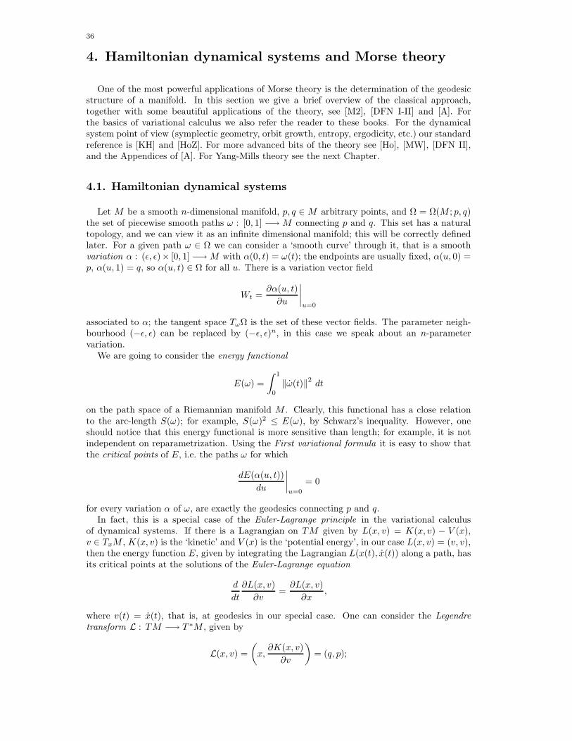
36

4. Hamiltonian dynamical systems and Morse theory

One of the most powerful applications of Morse theory is the determination of the geodesicstructure of a manifold. In this section we give a brief overview of the classical approach,together with some beautiful applications of the theory, see [M2], [DFN I-II] and [A]. Forthe basics of variational calculus we also refer the reader to these books. For the dynamicalsystem point of view (symplectic geometry, orbit growth, entropy, ergodicity, etc.) our standardreference is [KH] and [HoZ]. For more advanced bits of the theory see [Ho], [MW], [DFN II],and the Appendices of [A]. For Yang-Mills theory see the next Chapter.

4.1. Hamiltonian dynamical systems

Let M be a smooth n-dimensional manifold, p, q ∈ M arbitrary points, and Ω = Ω(M ; p, q)the set of piecewise smooth paths ω : [0, 1] −→ M connecting p and q. This set has a naturaltopology, and we can view it as an infinite dimensional manifold; this will be correctly definedlater. For a given path ω ∈ Ω we can consider a ‘smooth curve’ through it, that is a smoothvariation α : (ε, ε)× [0, 1] −→M with α(0, t) = ω(t); the endpoints are usually fixed, α(u, 0) =p, α(u, 1) = q, so α(u, t) ∈ Ω for all u. There is a variation vector field

Wt =∂α(u, t)∂u

∣∣∣∣u=0

associated to α; the tangent space TωΩ is the set of these vector fields. The parameter neigh-bourhood (−ε, ε) can be replaced by (−ε, ε)n, in this case we speak about an n-parametervariation.

We are going to consider the energy functional

E(ω) =∫ 1

0

‖ω(t)‖2 dt

on the path space of a Riemannian manifold M . Clearly, this functional has a close relationto the arc-length S(ω); for example, S(ω)2 ≤ E(ω), by Schwarz’s inequality. However, oneshould notice that this energy functional is more sensitive than length; for example, it is notindependent on reparametrization. Using the First variational formula it is easy to show thatthe critical points of E, i.e. the paths ω for which

dE(α(u, t))du

∣∣∣∣u=0

= 0

for every variation α of ω, are exactly the geodesics connecting p and q.In fact, this is a special case of the Euler-Lagrange principle in the variational calculus

of dynamical systems. If there is a Lagrangian on TM given by L(x, v) = K(x, v) − V (x),v ∈ TxM , K(x, v) is the ‘kinetic’ and V (x) is the ‘potential energy’, in our case L(x, v) = (v, v),then the energy function E, given by integrating the Lagrangian L(x(t), x(t)) along a path, hasits critical points at the solutions of the Euler-Lagrange equation

d

dt

∂L(x, v)∂v

=∂L(x, v)∂x

,

where v(t) = x(t), that is, at geodesics in our special case. One can consider the Legendretransform L : TM −→ T ∗M , given by

L(x, v) =(x,∂K(x, v)

∂v

)= (q, p);

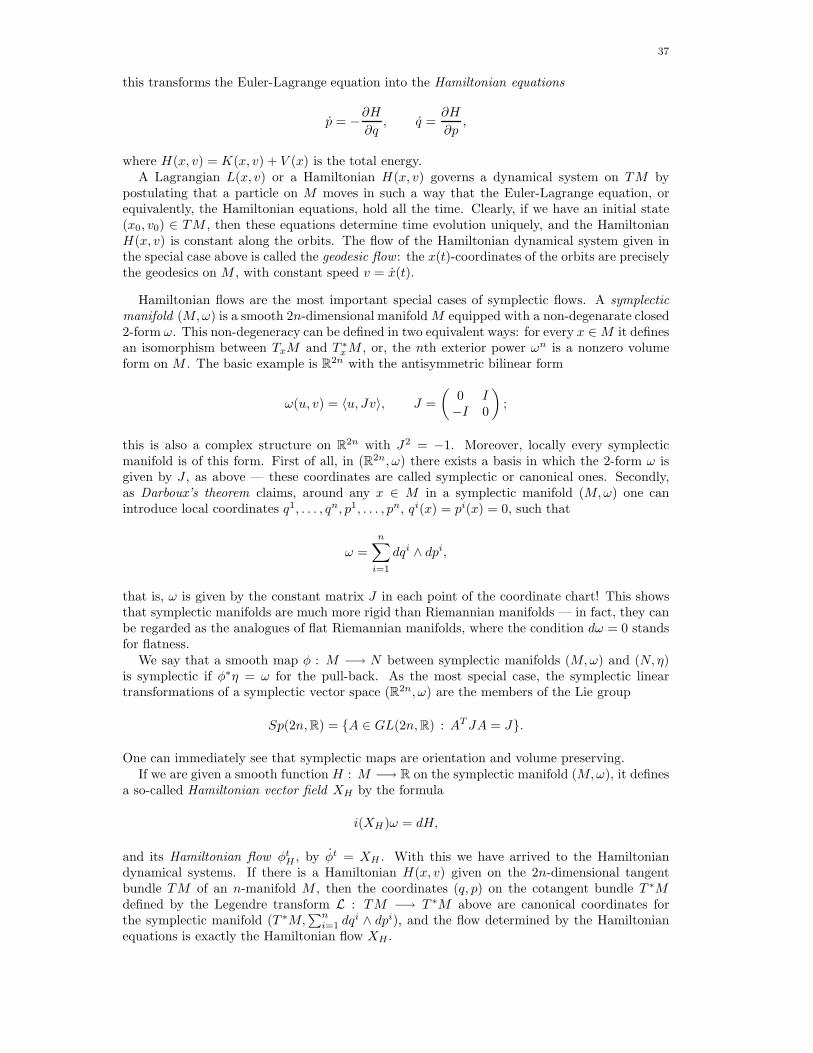
37

this transforms the Euler-Lagrange equation into the Hamiltonian equations

p = −∂H∂q

, q =∂H

∂p,

where H(x, v) = K(x, v) + V (x) is the total energy.A Lagrangian L(x, v) or a Hamiltonian H(x, v) governs a dynamical system on TM by

postulating that a particle on M moves in such a way that the Euler-Lagrange equation, orequivalently, the Hamiltonian equations, hold all the time. Clearly, if we have an initial state(x0, v0) ∈ TM , then these equations determine time evolution uniquely, and the HamiltonianH(x, v) is constant along the orbits. The flow of the Hamiltonian dynamical system given inthe special case above is called the geodesic flow : the x(t)-coordinates of the orbits are preciselythe geodesics on M , with constant speed v = x(t).

Hamiltonian flows are the most important special cases of symplectic flows. A symplecticmanifold (M,ω) is a smooth 2n-dimensional manifold M equipped with a non-degenarate closed2-form ω. This non-degeneracy can be defined in two equivalent ways: for every x ∈M it definesan isomorphism between TxM and T ∗

xM , or, the nth exterior power ωn is a nonzero volumeform on M . The basic example is R2n with the antisymmetric bilinear form

ω(u, v) = 〈u, Jv〉, J =(

0 I−I 0

);

this is also a complex structure on R2n with J2 = −1. Moreover, locally every symplecticmanifold is of this form. First of all, in (R2n, ω) there exists a basis in which the 2-form ω isgiven by J , as above — these coordinates are called symplectic or canonical ones. Secondly,as Darboux’s theorem claims, around any x ∈ M in a symplectic manifold (M,ω) one canintroduce local coordinates q1, . . . , qn, p1, . . . , pn, qi(x) = pi(x) = 0, such that

ω =n∑

i=1

dqi ∧ dpi,

that is, ω is given by the constant matrix J in each point of the coordinate chart! This showsthat symplectic manifolds are much more rigid than Riemannian manifolds — in fact, they canbe regarded as the analogues of flat Riemannian manifolds, where the condition dω = 0 standsfor flatness.

We say that a smooth map φ : M −→ N between symplectic manifolds (M,ω) and (N, η)is symplectic if φ∗η = ω for the pull-back. As the most special case, the symplectic lineartransformations of a symplectic vector space (R2n, ω) are the members of the Lie group

Sp(2n,R) = {A ∈ GL(2n,R) : ATJA = J}.

One can immediately see that symplectic maps are orientation and volume preserving.If we are given a smooth function H : M −→ R on the symplectic manifold (M,ω), it defines

a so-called Hamiltonian vector field XH by the formula

i(XH)ω = dH,

and its Hamiltonian flow φtH , by φt = XH . With this we have arrived to the Hamiltonian

dynamical systems. If there is a Hamiltonian H(x, v) given on the 2n-dimensional tangentbundle TM of an n-manifold M , then the coordinates (q, p) on the cotangent bundle T ∗Mdefined by the Legendre transform L : TM −→ T ∗M above are canonical coordinates forthe symplectic manifold (T ∗M,

∑ni=1 dq

i ∧ dpi), and the flow determined by the Hamiltonianequations is exactly the Hamiltonian flow XH .

38

It is worth noting that there exist even dimensional manifolds with no symplectic form; agood exercise is to show that the spheres S2n are such manifolds. Another exercise could be toconstruct symplectic flows which are not Hamiltonian.

On a symplectic manifold the Poisson bracket of functions is defined as {f, g} = ω(Xf , Xg).In canonical coordinates (q, p) this can be written in the form we met in Section 1.8:

f, g =n∑

i=1

∂f

∂qi

∂g

∂pi− ∂f

∂pi

∂g

∂qi.

The linear space C∞(M) is an infinite dimensional Lie algebra with Lie bracket {· , ·}, andX{f,g} = −[Xf , Xg]. A function f is invariant under the flow generated by a HamiltonianH , i.e. constant on orbits, iff {f,H} = 0 (for example, {H,H} = 0). These functions arecalled the first integrals of H , and the Poisson bracket of two first integrals is also a firstintegral. Noether’s theorem says that if H is invariant under a 1-parameter family of symplecticdiffeomorphisms generated by a Hamiltonian f , then f is a first integral of H . This theorem isusually quoted as ‘each symmetry of the system induces a quantity preserved during the motion’.There can be at most 2n − 1 first integrals with pointwise linearly independent derivatives.Liouville’s theorem states that Hamiltonian systems are completely integrable: if we can findn first integrals fi with {fi, fj} = 0, which are pointwise linearly independent on a joint levelset Mz = {x ∈ M : fi(x) = zi, i = 1, . . . n}, then ω|Mz = 0, Mz is invariant under eachHamiltonian flow φt

fi, and if Mz is compact and connected, then it is diffeomorphic to an n-

torus, and φtfi|Mz is conjugate to a linear flow via this diffeomorphism. This theorem also shows

that understanding Hamiltonian dynamics on tori is of crucial importance.

4.2. The Morse theory of geodesics

Returning to the geodesic flow and the variational calculus of geodesics, for a geodesic γ ∈ Ω,which is a critical point of E in the sense we described above, we can consider the Hessian ofE:

E∗∗(W1,W2) =∂2E(α(u1, u2, t))

∂u1∂u2

∣∣∣∣ui=0

,

where ∂α∂ui

(0, 0, t) = Wi(t). By the Second variation formula this is a well-defined symmetricbilinear form TγΩ × TγΩ −→ R. If γ is a minimal geodesic from p to q then E∗∗ is positivesemi-definite, i.e. the index of E is zero. A vector field Jt along a geodesic γ(t), t ∈ [0, 1], iscalled a Jacobi field if it satisfies the equation

∇2γ(t)Jt +R(γ(t), Jt)γ(t) = 0,

where R is the Riemann curvature tensor on M . This is exactly the equation appearing in theSecond variation formula. It is not too difficult to see that these Jacobi fields are exactly thevariation vector fields arising from free geodesic variations α of γ: the endpoints are not fixedand α(u, t) is a geodesic for each u. The endpoints p and q are called conjugate along γ if thereis a non-zero Jacobi field which vanish at t = 0 and t = 1. The multiplicity of this conjugacy isthe number of linearly independent Jacobi fields of this kind; this is at most n− 1 (an exercisefor the Reader). Note that the conjugacy of p and q does not mean that they can be connectedby lots of different geodesics — the non-trivial free geodesic variation has to vanish only in firstorder. An immediate corollary of the Second variation formula is that a vector field W1 ∈ TγΩbelongs to the null space of E∗∗ if and only if it is a Jacobi field, so the nullity of E∗∗ is equalto the multiplicity of p and q as conjugate points. A key result of the theory is the following:

Theorem 4.1. (Morse index theorem) The index of E∗∗ is equal to the number of pointsγ(t), 0 < t < 1, such that γ(t) is conjugate to γ(0) along γ; each conjugacy is counted withmultiplicity. This index is always finite. �

39

To visualize this theorem a good example can be a standard n-sphere with an antipodal pairof points, p and p∗, and a geodesic from p through p∗ to a third point q. The conjugacy of pand p∗ means an (n − 1)-dimensional nullspace of E∗∗ at the geodesic segment from p to p∗,and an (n − 1)-dimensional index at the geodesic from p to q: any geodesic from from p top∗ different from our original one, continued with the original geodesic segment from p∗ to q,results in a broken geodesic, which represents a kind of local maximum of E in the path spaceΩ(Sn; p, q).

Now we can define a natural metric on Ω(M ; p, q), using the metric ρ coming from theRiemannan structure of M : given ω, ω′ ∈ Ω with arc-lengths s(t), s′(t), then their distance is

d(ω, ω′) = max0≤t≤1

ρ(ω(t), ω′(t)) +(∫ 1

0

(s(t) − s′(t))2 dt)1/2

.

The second term is added in order to make E continuous. Now we can consider finite dimen-sional approximations to Ωa = {ω ∈ Ω |E(ω) ≤ a}, consisting of broken geodesics from p to q,and Theorem 0.2 gives our main result:

Theorem 4.2. (Fundamental theorem of Morse theory) Let M be a complete Riemann-ian manifold and let p, q ∈ M be two points which are not conjugate along any geodesic oflength ≤

√a. Then Ωa has the homotopy type of a finite cell complex, with one cell of dimen-

sion λ for each geodesic in Ωa at which E∗∗ has index λ. If p and q are not conjugate along anygeodesic, then Ω has the homotopy type of a countable cell complex, with cells correspondingto the indices of geodesics from p to q. �

We can apply this theory both to spaces of negative and positive curvature. Negative cur-vature is measured by the sectional curvatures (R(A,B)A,B), where A,B ∈ TpM . A minute’sthought about the defining equation of Jacobi vector fields shows that if (R(A,B)A,B) ≤ 0 forevery pair of tangent vectors A,B, then no two points of M are conjugate along any geodesic.On the other hand, we can consider the exponential map expp : TpM −→M , v �→ γv(1), whereγv(t) is the geodesic starting at p in the direction γv(0) = v, and it is not difficult to prove thatthe point expp(v) is conjugate to p along the geodesic γv if and only if the exponential mappingis critical at v. So we have the following corollary:

Theorem 4.3. (Cartan) SupposeM is simply connected complete Riemannian manifold, withsectional curvature (R(A,B)A,B) ≤ 0 everywhere. Then M is diffeomorphic to the Euclideanspace Rn.

Proof. There are no conjugate points, so by the Morse index theorem every geodesic segmenthas index 0. Thus Theorem 4.2 asserts that for each pair p, q ∈M the path space Ω(M ; p, q) hasthe homotopy type of a 0-dimensional cell complex, with one point for each geodesic from p to q.But then the simply connectedness of M implies that Ω(M ; p, q) is connected, so there is at mostone geodesic from p to q. On the other hand, M is complete, therefore we have shown that theexponential map expp is a bijection. Moreover, by the observations of the previous paragraphwe know that expp has no critical points, hence it is a local diffeomorphism. Combining theseresults we obtain that expp : TpM −→ M is a global diffeomorphism, which completes theproof. �

After showing that the exponential map is a covering map, a simpler solution to finish theproof could have been that the simply connectedness of M implies that it is diffeomorphic to itsuniversal cover, TpM . Nevertheless, the original argument give also the following more generalresult:

Corollary 4.4. If M is complete with nonpositive sectional curvature, then the homotopygroups πi(M) are zero for i > 1, and π1(M) is torsion-free. �

Inspite of the fact that no complete surface of constant negative curvature can be embeddedin R3, they do exist, and can be even compact: the compact factors of the hyperbolic plane

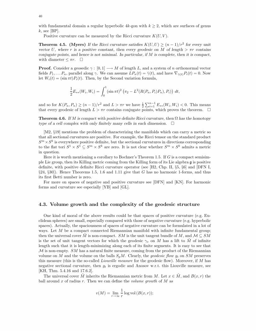
40

with fundamental domain a regular hyperbolic 4k-gon with k ≥ 2, which are surfaces of genusk, see [BP].

Positive curvature can be measured by the Ricci curvature K(U, V ).

Theorem 4.5. (Myers) If the Ricci curvature satisfies K(U,U) ≥ (n − 1)/r2 for every unitvector U , where r is a positive constant, then every geodesic on M of length > πr containsconjugate points, and hence is not minimal. In particular, if M is complete, then it is compact,with diameter ≤ πr. �

Proof. Consider a geosedic γ : [0, 1] −→M of length L, and a system of n orthonormal vectorfields P1, . . . Pn, parallel along γ. We can assume LPn(t) = γ(t), and have ∇γ(t)Pi(t) = 0. Nowlet Wi(t) = (sinπt)Pi(t). Then, by the Second variation formula,

12E∗∗(Wi,Wi) =

∫ 1

0

(sinπt)2(π2 − L2(R(Pn, Pi)Pn), Pi)

)dt,

and so for K(Pn, Pn) ≥ (n− 1)/r2 and L > πr we have 12

∑n−1i=1 E∗∗(Wi,Wi) < 0. This means

that every geodesic of length L > πr contains conjugate points, which proves the theorem. �

Theorem 4.6. If M is compact with positive definite Ricci curvature, then Ω has the homotopytype of a cell complex with only finitely many cells in each dimension. �

[M2, §19] mentions the problem of characterizing the manifolds which can carry a metric sothat all sectional curvatures are positive. For example, the Ricci tensor on the standard productSm×Sk is everywhere positive definite, but the sectional curvatures in directions correspondingto the flat tori S1 × S1 ⊆ Sm × Sk are zero. It is not clear whether Sm × Sk admits a metricin question.

Here it is worth mentioning a corollary to Bochner’s Theorem 1.5. If G is a compact semisim-ple Lie group, then its Killing metric coming from the Killing form of its Lie algebra g is positivedefinite, with positive definite Ricci curvature operator (see [H2, Chp. II, §5, §6] and [DFN I,§24, §30]). Hence Theorems 1.5, 1.6 and 1.11 give that G has no harmonic 1-forms, and thusits first Betti number is zero.

For more on spaces of negative and positive curvature see [DFN] and [KN]. For harmonicforms and curvature see especially [YB] and [GL].

4.3. Volume growth and the complexity of the geodesic structure

One kind of moral of the above results could be that spaces of positive curvature (e.g. Eu-clidean spheres) are small, especially compared with those of negative curvature (e.g. hyperbolicspaces). Actually, the spaciousness of spaces of negative curvature can be formulated in a lot ofways. Let M be a compact connected Riemannian manifold with infinite fundamental group;then the universal cover M is non-compact. SM is the unit tangent bundle ofM , and M ⊆ SMis the set of unit tangent vectors for which the geodesic γv on M has a lift to M of infinitelength such that it is length-minimizing along each of its finite segments. It is easy to see thatM is non-empty. SM has a natural finite measure, coming from the product of the Riemannianvolume on M and the volume on the balls SpM . Clearly, the geodesic flow gt on SM preservesthis measure (this is the so-called Liouville measure for the geodesic flow). Moreover, if M hasnegative sectional curvature, then gt is ergodic and Anosov w.r.t. this Liouville measure, see[KH, Thm. 5.4.16 and 17.6.2].

The universal cover M inherits the Riemannian metric from M . Let x ∈ M , and B(x, r) theball around x of radius r. Then we can define the volume growth of M as

v(M) = limr→∞

1r

log vol (B(x, r));

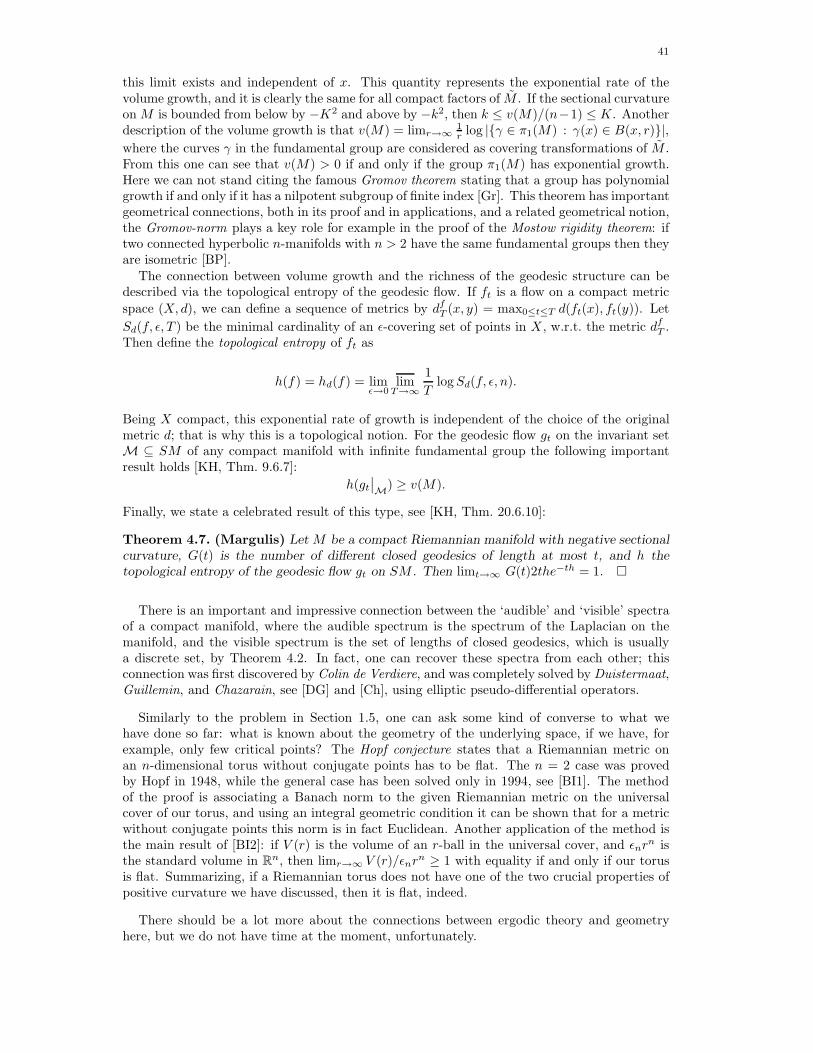
41

this limit exists and independent of x. This quantity represents the exponential rate of thevolume growth, and it is clearly the same for all compact factors of M . If the sectional curvatureon M is bounded from below by −K2 and above by −k2, then k ≤ v(M)/(n−1) ≤ K. Anotherdescription of the volume growth is that v(M) = limr→∞ 1

r log |{γ ∈ π1(M) : γ(x) ∈ B(x, r)}|,where the curves γ in the fundamental group are considered as covering transformations of M .From this one can see that v(M) > 0 if and only if the group π1(M) has exponential growth.Here we can not stand citing the famous Gromov theorem stating that a group has polynomialgrowth if and only if it has a nilpotent subgroup of finite index [Gr]. This theorem has importantgeometrical connections, both in its proof and in applications, and a related geometrical notion,the Gromov-norm plays a key role for example in the proof of the Mostow rigidity theorem: iftwo connected hyperbolic n-manifolds with n > 2 have the same fundamental groups then theyare isometric [BP].

The connection between volume growth and the richness of the geodesic structure can bedescribed via the topological entropy of the geodesic flow. If ft is a flow on a compact metricspace (X, d), we can define a sequence of metrics by df

T (x, y) = max0≤t≤T d(ft(x), ft(y)). LetSd(f, ε, T ) be the minimal cardinality of an ε-covering set of points in X , w.r.t. the metric df

T .Then define the topological entropy of ft as

h(f) = hd(f) = limε→0

limT→∞

1T

logSd(f, ε, n).

Being X compact, this exponential rate of growth is independent of the choice of the originalmetric d; that is why this is a topological notion. For the geodesic flow gt on the invariant setM ⊆ SM of any compact manifold with infinite fundamental group the following importantresult holds [KH, Thm. 9.6.7]:

h(gt

∣∣M) ≥ v(M).

Finally, we state a celebrated result of this type, see [KH, Thm. 20.6.10]:

Theorem 4.7. (Margulis) Let M be a compact Riemannian manifold with negative sectionalcurvature, G(t) is the number of different closed geodesics of length at most t, and h thetopological entropy of the geodesic flow gt on SM . Then limt→∞ G(t)2the−th = 1. �

There is an important and impressive connection between the ‘audible’ and ‘visible’ spectraof a compact manifold, where the audible spectrum is the spectrum of the Laplacian on themanifold, and the visible spectrum is the set of lengths of closed geodesics, which is usuallya discrete set, by Theorem 4.2. In fact, one can recover these spectra from each other; thisconnection was first discovered by Colin de Verdiere, and was completely solved by Duistermaat,Guillemin, and Chazarain, see [DG] and [Ch], using elliptic pseudo-differential operators.

Similarly to the problem in Section 1.5, one can ask some kind of converse to what wehave done so far: what is known about the geometry of the underlying space, if we have, forexample, only few critical points? The Hopf conjecture states that a Riemannian metric onan n-dimensional torus without conjugate points has to be flat. The n = 2 case was provedby Hopf in 1948, while the general case has been solved only in 1994, see [BI1]. The methodof the proof is associating a Banach norm to the given Riemannian metric on the universalcover of our torus, and using an integral geometric condition it can be shown that for a metricwithout conjugate points this norm is in fact Euclidean. Another application of the method isthe main result of [BI2]: if V (r) is the volume of an r-ball in the universal cover, and εnr

n isthe standard volume in Rn, then limr→∞ V (r)/εnrn ≥ 1 with equality if and only if our torusis flat. Summarizing, if a Riemannian torus does not have one of the two crucial properties ofpositive curvature we have discussed, then it is flat, indeed.

There should be a lot more about the connections between ergodic theory and geometryhere, but we do not have time at the moment, unfortunately.

42

4.4. Morse theory on symplectic manifolds

This section consists of two parts. First of all, recall Noether’s theorem from Section 4.1,showing the importance of the symmetries of a Hamiltonian system. So let us suppose that Gis a Lie group which acts on the symplectic manifold M and preserves the symplectic form ω.Each element a ∈ g in the Lie algebra of G determines a one-parameter symplectic flow in M ,with Hamiltonian Ha. Now we have

H[a,b] = {Ha, Hb} + C(a, b),

where C(a, b) is a constant satisfying

C([a, b], c) + C([b, c], a) + C([c, a], b) = 0,

i.e. it is a 2-cocycle of g. The action of G is called a Poisson action if H[a,b] = {Ha, Hb} always.In this case the map px(a) = Ha(x) is a Lie-algebra homomorphism, and we can define theso-called moment map

P : M −→ g∗, P (x) = px.

This map is G-equivariant, and so if H is a Hamiltonian function that is invariant under G, thenP is a first integral of H . Note that G acts on P−1(0), and under some natural conditions thequotient N = P−1(0)/G is a smooth symplectic manifold. The point of this construction, calledsymplectic reduction, is that this N represents exactly the so called stable points of M under theaction of G, which means that the G-invariant functions on M are in a 1-to-1 correspondancewith the functions on N . The significance of this theorem, proved by Morse theory, is thatit is not always clear how one can ‘see’ the G-invariant functions on a manifold. The Readeris encouraged to construct some pathological examples. The name of this topic is geometricinvariant theory; for more on symplectic reduction see [A, Appendix 5], [MΦ], [Se]. We will seean application to Yang-Mills theory in Section 5.3.

In the Introduction 0.2 we encountered the problem of relating the number of fixed pointsof certain diffeomorphisms to the number of critical points of a Morse function on the samemanifold.

Let Diff0(M,ω) be the identity component of the group of all symplectic diffeomorphismsof a symplectic manifold (M,ω). It is proven by A. Banyaga that the commutator subgroupof Diff0(M,ω) consists precisely of the symplectomorphisms generated by a time-dependentHamiltonian flow. In [A, Appendix 9] there is an outline of the result that if such a symplec-tomorphism is close enough to the identity, then the statement about the number of its criticalpoints is true. As a special case we can consider the measure-preserving diffeomorphisms of thetorus T2. Being in Diff0(M,ω), on the covering space R2 it must be of the form

ψ : x �→ x+ f(x), x ∈ R2,

with a periodic function f . As claimed in [A], and proved in [CZ], being in the commutatorgroup is equivalent to the condition that [f ] =

∫T2 f(x) dx = 0. So the above mentioned theorem

applies for such torus maps. Arnold conjectured that the condition of closeness to identity canbe dropped. For the standard symplectic manifolds T2n it is proved by Conley and Zehnder in[CZ], and for more general symplectic manifolds by A. Floer, see [F], [HoZ], [Ho].

43

5. The Yang-Mills theory of connexions

This chapter is to briefly overview Morse theoretical methods in relating connexions in vectorbundles to the topology of the bundles, from characteristic classes to Yang-Mills theory.

5.1 Characteristic classes and the Gauss-Bonnet-Chern theorem

It is a well-known sentence that ‘curvature has strong topological consequences’. Of this wehave already seen some examples: the Gauss-Bonnet theorem in the Introduction 0.2, somegeometric group theory in Section 1.10, and some dynamical system approaches in Chapter4. Inspired by these results, and by the ideas around Theorems 1.1 and 1.4, one might thinkit helpful to use connexions and curvature to define topological invariants of bundles. Thebeautiful and useful theory of characteristic classes of vector bundles is invented by Stiefel,Whitney, Pontryagin and Chern to fulfill this ambition. To give the main idea, we begin withthe special case of unitary complex line bundles over a compact manifold M .

The Lie algebra of the structure group U(1) can be identified with the imaginary numbersiR, thus the curvature of a connexion A can be written as FA = −2πiφ for a real 2-form φ,that is closed because of the Bianchi identity dAFA = 0. Taking another connexion A′ = A+a,a ∈ Ω1(M ; iR), we have FA′ = FA+da, so [φ′] = [φ] ∈ H2(M) in deRham cohomology. Thus wehave a cohomology class that is independent of the chosen connexion, i.e. it is a characteristicof the line bundle itself. That is why it is called a characteristic class.

Now let us consider invariant polynomials in n2 complex variables, written as functionson complex n × n matrices; the invariance of a polynomial p means p(gAg−1) = p(A) forall A ∈ Mn(C), g ∈ GLn(C). We will restrict ourselves to homogeneous polynomials. Themain examples come from the characteristic polynomial σ(t) = det(I + tA) =

∑ni=0 σi(A)ti,

and s(t) = −t ddt log(det(I − tA)) =

∑∞k=0 sk(A)tk: each of the functions σi(A) and sk(A)

is an invariant polynomial. Clearly, σ1(A) = s1(A) = Tr(A). It is not difficult to see thatsk(A) = Tr(Ak) and that there exist polynomials Qk, Pk ∈ Q[x1, . . . , xk] such that sk(A) =Qk(σ1(A), . . . , σk(A)) and σk(A) = Pk(s1(A), . . . , sk(A)). The effects of matrix operations aregiven by σk(A1 ⊕A2) =

∑ki=0 σi(A1)σk−i(A2), sk(A1 ⊕A2) = sk(A1) + sk(A2), sk(A1 ⊗A2) =

sk(A1) · sk(A2). For diagonal matrices D = diag(λ1, . . . , λn), the polynomial σk(D) becomesthe kth elementary symmetric polynomial in the variables λ1, . . . , λn. Hence, the fundamentaltheorem of symmetric polynomials, together with the fact that diagonalizable matrices aredense in Mn(C), give that every (homogeneous) invariant polynomial can be written as a(homogeneous) polynomial of the σi’s. Thus, our examples of invariant polynomials are in factthe most important ones.

Finally, we define an almost invariant polynomial, the Pfaffian Pf : so(2n,R) −→ R, byω(A) ∧ · · · ∧ ω(A) = n! Pf (A)Vol, where ω(A) =

∑i<j Aijei ∧ ej ∈ Λ2(R2n), and Vol =

e1 ∧ · · · ∧ e2n. For instance, for the block diagonal matrix D = diag(a1J0, . . . , anJ0), whereJ0 is the standard 2-dimensional symplectic matrix, we have Pf(A) = a1 · · · an. Furthermore,for A ∈ so(2n,R) and B ∈ Mn(C), we have Pf(A)2 = det(A) and Pf(BABT ) = Pf(A) det(B).Taking the realification map sun −→ so2n, A �→ AR, we get Pf(AR) = (−i)n det(A).

Now we are going to evaluate these polynomials on the End(E)-valued curvature forms FA

of a rank-m complex vector bundle E −→ M , where M is a compact smooth manifold, seeSection 1.2. First of all, ∧ is commutative on even-dimensional differential forms, so if p is ahomogeneous invariant polynomial of degree k, and Aij ∈ Ω2(M ;E), 1 ≤ i, j ≤ m, then wecan speak of p(A) ∈ Ω2k(M ;E). If we have a connexion in E, given locally by the 2-forms Aτ ,then the invariance of p gives a globally defined 2k-form p(FA). If E′ is an isomorphic vectorbundle, then using that isomorphism, we get a connexion A′ in E′ corresponding to A in E,and we have p(FA) = p(FA′), up to the isomorphism. From this the following basic facts canbe deduced: p(FA) is always a closed form, and its de Rham cohomology class is independent

44

of the chosen connexion A. In particular, using the flat connexion in trivial vector bundles, wesee that [p(E)] = 0 if E is trivial. And we can define the topological invariants, the kth Chernclass of any bundle E by

ck(E) =[σk

(−12πi

FA

)]∈ H2k(M ; C),

and the kth Chern character class by

chk(E) =1k!

[sk

(−12πi

FA

)]∈ H2k(M ; C).

We have c0(E) = 1, ch0(E) = dimE, c1(E) = ch1(E), ch2(E) = 12c1(E)2 − c2(E), for in-

stance. The normalization in the definition suggests that we should have some nice numbersfor certain nice bundles. Indeed, some computation in the Fubini-Study metric of CP

1, the iso-morphism H2(CP

n; C) � H2(CP1; C), and the integration isomorphism I : H2(CP

n; C) −→ C

give I(c1(Hn)) = −1 for the tautological line bundle Hn = On(−1) of Section 1.1.Actually, Chern classes can also be defined as the unique family of cohomology classes ck(E) ∈

H2k(M ; C) satisfying the three conditions(i) I(c1(H1)) = −1, ck(Hn) = 0 when k > 1, and c0(Hn) = 1(ii) f∗ck(E) = ck(f∗(E))(iii) ck(E1 ⊕ E2) =

∑ki=0 ci(E1)ck−i(E2).

Note that all Chern classes lie in R-cohomology. The uniqueness part of the theorem followsfrom the extremely useful splitting principle: for any complex vector bundle E on M thereexists a manifold T and a proper smooth map f : T −→M such that f∗ : Hk(M) −→ Hk(T )is injective and f∗(E) � γ1 ⊕ · · · ⊕ γn for certain complex line bundles γi. There is a similarresult for real vector bundles, too.

If E is a real rank-2k oriented vector bundle over M , with inner product 〈·, ·〉, then inorthogonal trivializations the curvature 2-forms FAτ of a metric connexion A = {Aτ} are skew-symmetric, the transition maps of the bundle are in SO(2k,R), so, with the help of the Pfaffian,we can define a global real 2k-form

e(E) =[Pf

(FA

2π

)]∈ H2k(M ; R),

the so-called Euler class of the bundle E. Also, if E is a complex rank-k Hermitian vectorbundle, then e(E) := e(ER), and e(E) = ck(E). We have e(E1 ⊕ E2) = e(E1)e(E2) ande(E∗) = −e(E). Note that almost every textbook has its own sign conventions and signmistakes in the theory of characteristic classes. I did my best to be correct and precise, but fullsuccess cannot be guaranteed.

A main example is the tangent bundle of a 2-dimensional compact Riemannian manifold Σembedded isometrically into R3 with the Levi-Civita connexion A. By the computation of FA

at the end of Section 1.2, we have e(TΣ) = KVolΣ/(2π). So the Gauss-Bonnet theorem can bereformulated as I(e(TΣ)) = χ(Σ).

Recall that once we have already defined the first Chern classes C1(E) ∈ Z for complexvector bundles over closed oriented surfaces Σ in Section 1.1. These numbers behave wellunder the usual vector bundle operations, and we have I(c1(On(k))) = k = C1(On(k)), so theuniqueness of the Chern class gives I(c1(E)) = C1(E) for all complex bundles E on Σ. Letus see another check of the compatibility of the two definitions. An almost complex structureon the real bundle TΣ can be integrated to give an honest complex line bundle, for whichC1(TΣ) = χ(Σ) can be computed via Morse-Poincare-Hopf index theory and Theorem 1.1. Andthis is the same as the above-mentioned form of the Gauss-Bonnet theorem. Unfortunately,I do not know a transparent explanation on the equality of the ‘homotopical Chern classes’

45

C1(E) ∈ π1(GL(n,C)) and the ‘homological Chern classes’ c1(E) ∈ H2(Σ). Neither am I awareof a homotopical description of higher Chern classes.

Let E be a real rank-m vector bundle over the n-dimensional manifold M . The Thomisomorphism theorem claims the existence of an isomorphism Φ : Hq(M) −→ Hm+q

c (E) suchthat U = Φ(1) ∈ Hm(E), the so-called Thom class, has integral 1 over each fiber Ep. Note thatthe isomorphism of the cohomology groups follows also from the Poincare duality theorem ofthe Introduction 0.2. Let us define e(E) by Φ(e(E)) = U ∧U . Now a unicity theorem similar tothe one about the Chern classes yields that for oriented bundles E we have e(E) = e(E). Thesignificance of e(E) lies in the fact that for an arbitrary smooth section s : M −→ E we havee(E) = s∗(U), which makes it possible to connect the local data at the zeros of a section to theglobal topological data of the Euler class. If the real rank of E and dimM coincide, we candefine the indices ι(s, p) ∈ {±1} for any section s that is transversal to the zero section s0 at allits zeros. Now the main result is I(e(E)) =

∑p ι(s; p), which, together with the Poincare-Hopf

index theorem, gives the following generalization of the Gauss-Bonnet theorem for orientedcompact manifolds: ∫

M

e(TM) = χ(M).

Let us finally examine the class ch2(E) for complex bundles with structure group SU(n).Since the Lie algebra sun consists of traceless matrices, we have c1(E) = 0, and so ch2(E) =−c2(E). By definition, ch2(E) =

[1

8π2 Tr(FA ∧ FA)]∈ H4(M ; C), therefore we have

C2(E) =∫

M

c2(E) =−18π2

∫M

Tr(FA ∧ FA) ∈ Z

for SU(n)-bundles.

One of the main applications of the theory is to (co-)bordism. For instance, CP2n is not

the boundary of any compact manifold N . For one computes ck(TCPn) = (−1)k(n+1

k

)c1(Hn)k,

from where the existence of a closed 2n-form ω follows with 0 =∫

CPn ω =∫

∂N ω =∫

N dω = 0,a contradiction.

Another application is to enumerative algebraic geometry, such as Bezout’s theorem on thenumber of intersection points of two algebraic curves.

For more on characteristic classes see [MS] first of all, and also [DFN III], [KN II], [MT],[BT].

5.2. The YM functional and its critical points

Given a Riemannian manifold M , which of the metric connexions has the least curvature?And which metric has a metric connexion with the global minimum of the curvature? If wewant to measure the total average curvature, then the Gauss-Bonnet-Chern theorem says thatall metrics and all connexions are the same: the integral is a topological invariant. That is,a real question is to identify the manifolds which can carry a flat Riemannian metric. For2-manifolds with χ(M) = 0 the only possibility is the torus. For flat Riemannian manifolds ofarbitrary dimension see [KN I, Note 5]. In more generality, the above questions can be askedabout complex vector bundles E −→ M with Hermitian inner products. For this problem wewill introduce the Yang-Mills functional, which is to measure the economicity of connexions.For more see [Se], [AB2], [DFN I-II], [MΦ], [N], [DK].

The Yang-Mills functional is defined on the set of unitary connexions A(E) as

YM(A) =−18π2

∫M

Tr(FA ∧ ∗FA),

where ∗ is the Hodge star operator, and we used the invariant inner product 〈A,B〉 = −Tr(AB)on the compact Lie algebra of skew-hermitian matrices. (That is, we could consider a bundle

46

with an arbitrary compact structure group G, and Lie algebra g.) Being the connexions unitary,YM(A) ∈ R≥0, and it is clear that YM(A) = 0 if and only if A is a flat connexion. Let G bethe group of unitary bundle automorphisms of E — this is the gauge group, which acts on Aby Aτ �→ Ad(g−1)Aτ − dg · g, and so FA �→ Ad(g−1)FA, which means that the YM functionalis G-invariant. In Theorem 1.3 we identified A(E) with the space C(E) of all holomorphicstructures, on which the complex gauge group GC of all bundle isomorphisms acts. So A/GC isthe space of isomorphism classes of holomorphic structures on E. Note that the definition ofYM does not contain the Hermitian i.p. of E, only the Riemannian metric of M .

The Euler-Lagrange variation of the YM functional gives that the critical points of thefunctional are the connexions of constant curvature: dA ∗ FA = 0. They are characterized bythe property that dAξ = 0 for ξ ∈ Ω0(M ; End(E)) is equivalent to Tγξ(x1) = ξ(x2)Tγ , where Tγ

is the parallel transport along the curve γ from x1 to x2. In a bundle with a constant curvatureconnexion A, there is a splitting of E into subbundles E(λ) according to the eigenvalues λ ofthe operator ∗FA. In each such subbundle the curvature ∗FA acts as the scalar λ, so the firstChern class can easily be computed, and

λ =−2πi

Vol(M)C1(E(λ))dim(E(λ))

,

where the ratio C1(E(λ))/ dim(E(λ)) is called the slope of E(λ).Every connexion satisfies the Bianchi identity dAFA = 0, hence the so-called self-dual and

anti-self-dual connexions ∗FA = ±FA satisfy the equation dA ∗ FA = 0, too. So if they havefinite energy YM(A) < ∞, then they are critical points of the functional, and are called theinstanton and anti-instanton solutions of the YM equation. Note that any critical point of thefunctional has YM(A) ≥ |C2(E)|, with equality for the instanton and anti-instanton solutions.So they are the absolute minima of the YM functional (if they exist). Are there other criticalpoints?

Theorem 5.1. Let L be a holomorphic line bundle over the closed Riemann surface Σ witha given Riemannian metric. Then there is a Hermitian inner product h in L, unique up toa constant multiple, whose curvature (i.e. the curvature of the unique connexion compatiblewith both the holomorphic structure and the inner product) is constant. This inner productminimizes the YM functional on unitary connexions compatible with the holomorphic structureof L. �

Note that the constant curvature connexions are originally the critical points of the YM onthe set A(L, h), with fixed Hermitian i.p. h, without a holomorphic structure, and now theyhave been found to be the minima of the ‘orthogonal’ sets.

Corollary 5.2. If a holomorphic line bundle L on Σ has a non-zero holomorphic section, thenc1(L) ≥ 0. �

5.3. Holomorphic line bundles and the Narasimhan-Seshadri theorem

Theorem 5.3. (Birkhoff - Grothendieck) The holomorphic line bundles over a com-plex manifold M form a group under ⊗, which is isomorphic to H2(M ; Z), and thereforeparametrized by the first Chern class of the bundle. Every holomorphic vector bundle over CP

1

is a direct sum of holomorphic line bundles, where the decomposition is basically unique.

It would be nice to prove Theorem 5.1 for arbitrary holomorphic vector bundles, but thisgeneralization simply would not be true, only for ‘almost all’ vector bundles. As we saw inthe previous section, if there is a constant curvature connexion, then we can decompose thebundle into holomorphic subbundles, so we can restrict ourselves to indecomposable bundles.

47

A holomorphic bundle E is called stable if its every holomorphic subbundle has strictly smallerslope than E. Such a bundle is of course indecomposable.

Theorem 5.4. (Narasimhan - Seshadri) A holomorphic bundle E over Σ is stable iff itis indecomposable and has an i.p. whose curvature is constant and scalar. In particular, aholomorphic SU(n)-bundle is stable iff it has a flat connexion. �

Let us finally see the connection to the symplectic invariant theory of Section 4.4. Let Σ bea Riemann surface, and E the trivial complex rank-2 vector bundle over it. Then the spaceA(E) is Ω1(Σ; su2), on which the bilinear YM functional YM(α, β) is a symplectic form. Thegauge group G = {g : Σ −→ SU(2)} leaves this YM form invariant, and the correspondingmoment map is the curvature F : Ω1(Σ; su2) −→ Ω2(Σ; su2). The factor space F−1(0)/G is theset of isomorphism classes of flat connexions, and symplectic invariant theory says that this isthe space of stable points. Thus we have arrived to the special case of Theorem 5.4.

5.4. Some physics

In electrodynamics, the pseudo-Riemannian base manifold M is the Minkowski space-timeR3 ×R, a connexion A in TM is the potential, the curvature FA is the intensity of the electro-magnetic field. The Bianchi identity and the Yang-Mills equation are the Maxwell equations.

In the Standard Model of quantum physics, we have a complex vector bundle over the space-time M with structural group G = SU(3) × SU(2) × U(1). The sections of this vector bundleare the fermions, the connexions in the bundle are the bosons, and the curvature of a connexionis the Yang-Mills field intensity.

In the past few years there has been a revolution in 4-dimensional (symplectic) topology,mainly dew to Seiberg and Witten who showed the connection between the physics of Yang-Mills fields and geometry. Recently it turned out the theory of the Donaldson-, the Gromov-,and the Seiberg-Witten-invariants are equivalent, but there is still a lot to understand.

A second trail towards physics is mirror symmetry for Calabi-Yau manifolds, which comesfrom string theory.

For more see [MΦ], [N], [DK], [T], and [As].

48

6. Discrete Morse theory

As it has been shown by the recent work of Robin Forman, almost all of the Morse theorywe have seen in this essay has a discrete counterpart for simplical and cell complexes. Thisdiscrete theory seems to have the same geometric depth, while some results are considerablyeasier to prove. Moreover, it also has some interesting corollaries to combinatorial problems.The basic paper by Forman is [Fo1]; for a nice survey see [Fo2].

Let K be the set of non-empty simplices of a finite simplicial complex Mn. We writeα(p) ∈ K(p) for p-dimensional simplices, and α > β for the face relation. A function f : K −→ R

is a discrete Morse function iff for every α(p) ∈ K

(i) |{β(p+1) > α : f(β) ≤ f(α)}| ≤ 1, and(ii) |{γ(p−1) < α : f(γ) ≥ f(α)}| ≤ 1.

It is easy to see that for every simplex α(p) at least one of the sets in (i) or (ii) is empty.A simplex α(p) is critical with index p iff both sets are empty. Any discrete Morse function fdefines a disjoint collection V of pairs of simplices:

Vf = {(α(p), β(p+1)) : α < β, f(β) ≤ f(α)}.

This matching is called the discrete gradient vector field of f , and a simplex is critical iff it isnot contained in any of the pairs of V . In general we call a matching of ‘neighbouring simplices’a discrete vector field.

If V is a discrete vector field, then a V -path of dimension p is a sequence of simplicesα

(p)0 , β

(p+1)0 , α

(p)1 , . . . , β

(p+1)k−1 , α

(p)k such that (αi, βi) ∈ V for all i = 0, 1, . . . , k, and βi > αi+1 =

αi. We say that a V -path is closed if αk = α0. The analogue of Smale’s gradient like vector fieldsis much simpler here: a vector field V is the gradient vector field of a discrete Morse functioniff there are no closed V -paths. Moreover, the discrete version of the cancellation theorem usedin the h-cobordism Theorem 0.6 is rather obvious: if the simplices α(p) and β(p+1) are criticalfor the Morse function f , and there is exactly one gradient path from ∂β to α, then there isanother Morse function g with the same critical simplices except that α and β are no longercritical. Moreover, the gradient vector field of g coincides with the gradient field of f exceptalong the unique gradient path from ∂β to α.

The basic results of Morse theory, Theorems 0.2 and 0.3 are also valid, with simplicialcollapsing in place of the homotopy and diffeomorphic equivalences. Even the Smale-Witten-Floer-Schwarz-type representation of the cohomology of M by the Morse complex is not verydifficult to prove: the main help that we did not have in the smooth category is the existenceof the map Φ∞, which is something like the limit of the gradient flow Φ at time t = ∞; thesethings will be defined now.

We can think of the gradient vector field V as a map from p-simplices to (p+ 1)-simplices.If we set the sign of V (α(p)) such that 〈α, ∂V (α)〉 = −1 with the canonical inner product onoriented chains, then we have a linear extension V : Cp(M ; Z) −→ Cp+1(M ; Z). Now definethe discrete-time flow Φ : Cp(M ; Z) −→ Cp(M ; Z) by

Φ = 1 + ∂V + V ∂.

This Φ is worth calling the flow of V , since in the smooth category Cartan’s formula saysdi(V ) + i(V )d = LV , and LV ∼ ΦV − 1 approximately. If α(p) is not a critical simplex, thenΦ(α) is a p-chain consisting entirely of oriented p-simplices on which f is less than f(α), so,loosely speaking, Φ decreases f — just like the gradient flow in the smooth case. But it is animportant difference that the iterates of Φ stabilize in finite time: there is a positive integer Nsuch that

ΦN = ΦN+1 = · · · = Φ∞.

49

Let CΦp ⊆ Cp(M ; Z) be the set of Φ-invariant p-chains. As Φ∂ = ∂Φ, we have a chain complex

CΦ : 0 −→ CΦn

∂−→CΦn−1

∂−→ . . . .

The main result is that Φ∞ : C∗(M ; Z) −→ CΦ∗ induces an isomorphism on homology. The

chain complex CΦ∗ is called the Morse complex, since Φ∞ establishes a 1-to-1 correspondence

between Mp and CΦp for all p, where Mp is the set of critical indices of dimension p. Thus we

have the Morse complex

M : 0 −→ Mn∂−→Mn−1

∂−→ . . . ,

with ∂ = (Φ∞)−1∂Φ∞, andH∗(M) = H∗(M ; Z).

Just as in Witten’s theory, the boundary operator can be given directly: for any critical β(p+1),

∂β =∑

critical α(p)

n(α, β)α,

wheren(α, β) =

∑α(p)

〈∂β, α〉∑

γ∈Γ(α,α)

m(γ),

where Γ(α, α) is the set of gradient paths from α to α, and m(γ) ∈ {±1}, according to anorientation matter just as in Witten’s theory.

Finally, we have to note that inspite of the relative simplicity of discrete Morse theory, itimplies the smooth theory.

In [Fo3] there is an application to evasive graph properties. Consider a game with twoplayers, called the hider and the seeker. Let M be a subcomplex of the simplex Δn, knownto both of the players, and the hider choses a simplex σ of Δn. The seeker can ask questionsof the form ‘is the vertex xi in σ?’, and wants to find out whether σ is in M , with the leastpossible number of questions. For any decision tree algorithm A, we denote by Q(σ,A,M) thenumber of questions asked by the seeker before he/she reaches his/her goal. The complexity ofM is defined by

c(M) = infA

supσQ(σ,A,M).

M is called evasive if c(M) = n + 1, the worst possible value. It is known e.g. that if M isnonevasive then it is collapsible, and so contractible. If M is evasive, then for any A there existsimplices σ with Q(σ,A,M) = n+1; they are called the evaders of A. The main result of [Fo3]is that for any decision tree algorithm A, the number of evaders is e(A) ≥ b(M), the sum ofthe Betti numbers of the manifold.

A monotone graph property M on n vertices is a subcomplex of Δ(n2), such that the auto-

morphism group of M acts transitively on the vertices of M . There is a conjecture by Rivest,Vuillemin and Karp that every such subcomplex M of a simplex Δm is evasive. It is known tobe true for m a prime power. It would be nice to prove the conjecture using a Morse theorywith group actions.

50

References

[AG] L. Alvarez-Gaume: Supersymmetry and the Atiyah-Singer index theorem, Commun.Math. Phys. 90 (1983), 161-173.

[A] V. I. Arnold: Mathematical methods of classical mechanics (in Hungarian), MuszakiKonyvkiado, Budapest, 1985.

[As] P. S. Aspinwall: String theory and duality, Proceedings of the ICM’98, Berlin Vol. II,229-238.

[AB1] M. F. Atiyah – R. Bott: A Lefschetz fixed point formula for elliptic complexes I-II,Ann. Math 86, 88 (1967, 1968), 374-401., 451-491.

[AB2] M. F. Atiyah – R. Bott: The Yang-Mills equations over Riemann surfaces, Phil. Trans.Royal Soc. London A 308 (1982), 523-615.

[BP] R. Benedetti – G. Petronio: Lectures on hyperbolic geometry, Springer-Verlag, Berlin,1992.

[BGV] N. Berline – E. Getzler – M. Vergne: Heat kernels and Dirac operators, Grundlehrender mat. Wiss. 298, Springer-Verlag, Berlin, 1992.

[B] R. Bott: Morse theory indomitable, Publ. Math. d’I.H.E.S. 68 (1988), 99-117.[BT] R. Bott – L. W. Tu: Differential forms in algebraic topology, GTM 82, Springer-Verlag,

New York, 1982.[Br] R. Brooks: Constructing isospectral manifolds, Amer. Math. Monthly 95 (1988), 823-839.

[BI1] D. Burago – S. Ivanov: Riemannian tori without conjugate points are flat, Geom. Funct.Anal. 4 (1994), 259-269.

[BI2] D. Burago – S. Ivanov: On asymptotic volume of tori, Geom. Funct. Anal. 5 (1995),800-808.

[Ch] J. Chazarain: Spectre des operateurs elliptiques et flots hamiltioniens, LNM 514, Springer-Verlag, Berlin, 1976.

[CZ] C. C. Conley – E. Zehnder: The Birkhoff-Lewis fixed point theorem and a conjectureof V.I. Arnold, Invent. Math. 73 (1983), 33-49.

[DMS] P. Di Francesco – P. Mathieu – D. Senechal: Conformal field theory, Springer-Verlag,New York, 1997.

[DK] S. K. Donaldson – P. B. Kronheimer: The geometry of 4-manifolds, Oxford UniversityPress, 1990.

[DFN] B. A. Dubrovin – A. T. Fomenko – S. P. Novikov: Modern geometry — methods andapplications I-III., GTM 93, 104, 124, Springer-Verlag, New York, 1984, 1985, 1990.

[DG] J. J. Duistermaat – V. W. Guillemin: The spectrum of positive elliptic operators andperiodic bicharacteristics, Invent. Math. 29 (1975), 39-79.

[EK] J. Eells, Jr. – N. H. Kuiper: Manifolds which are like projective planes, Publ. Math. d’I.H.E.S. 14 (1962), 5-46.

[F] A. Floer: Morse theory for Lagrangian intersections, J. Diff. Geometry 28 (1988), 513-547.[Fo1] R. Forman: Morse theory for cell complexes, Adv. in Math. 134 (1998), 90-145.[Fo2] R. Forman: Combinatorial differential topology and geometry (New perspectives in alge-

braic combinatorics, Berkeley, CA, 1996-97), Math. Sci. Res. Inst. Publ., 38, CambridgeUniversity Press, Cambridge, 1999. 177-206. See also http://www.math.rice.edu/~forman

[Fo3] R. Forman: Morse theory and evasiveness, Combinatorica 20 (2000), no. 4, 489-504.[FH] W. Fulton – J. Harris: Representation theory, GTM 129, Springer-Verlag, New York,

1991.[G] P. B. Gilkey: Invariance, the heat equation and the Atiyah-Singer index theorem, CRC

Press, Boca Raton, 1995.

51

[GH] P. Griffiths – J. Harris: Principles of algebraic geomery, John Wiley & Sons, New York,1978.

[Gr] M. Gromov: Groups of polynomial growth and expanding maps, Publ. Math. I.H.E.S. 53(1981), 53-73.

[GrL] M. Gromov – B. Lawson: Positive scalar curvature and the Dirac operator on completeRiemannian manifolds, Publ. Math. I.H.E.S. 58 (1983), 295-408.

[H1] S. Helgason: Differential geometry and symmetric spaces, Academic Press, New York,1962.

[H2] S. Helgason: Differential geometry, Lie groups and symmetric spaces, Academic Press,New York, 1978.

[Ha] G. Halasz: The Selberg trace formula (in Hungarian), Lecture notes, Bolyai Kollegium,Budapest, 1998. http://www.math-inst.hu/~major

[Ho] H. Hofer: Dynamics, topology, and holomorphic curves, Proceedings of the ICM’98 BerlinVol. I., 255-280.

[HoZ] H. Hofer – E. Zehnder: Symplectic invariants and Hamiltonian dynamics, BirkhauserAdvanced Texts, Basel Textbooks, Birkhauser Verlag, Basel, 1994.

[Hu] W. Huang: On closed 4-manifolds admitting a Morse function with 4 critical points,Czechoslovak Math. J. 46(121) (1996), 47-59.

[KH] A. Katok – B. Hasselblatt: An introduction to the modern theory of dynamical systems,Cambridge University Press, Cambridge, 1995.

[KN] S. Kobayashi – K. Nomizu: Foundations of differential geometry I-II., John Wiley &Sons Interscience, New York, 1963, 1969.

[L] S. Lang: Differential and Riemannian manifolds, GTM 160, Springer-Verlag, New York,1995.

[Li] R.L. Liboff: Introductory Quantum Mechanics, Addison Wesley Longman, Reading, 1998.

[Lu] A. Lubotzky: Discrete groups, expanding graphs and invariant measures, Progress inMath. 125, Birkhauser Verlag, Basel, 1994.

[MT] I. Madsen – J. Tornehave: From calculus to cohomology, Cambridge University Press,Cambridge, 1997.

[Ma] C. R. F. Maunder: Algebraic topology, Dover Publications, Mineola, NY, 1996.[MW] J. Mawhin – M. Willem: Critical point theory and Hamiltonian systems, Applied

Math. Sci. 74, Springer Verlag, New York, 1989.[M1] J. Milnor: On manifolds homeomorphic to the 7-sphere, Ann. of Math. 64 (1956), 399-405.[M2] J. Milnor: Morse theory, Annals of Math. Studies 51, Princeton University Press, Prince-

ton, 1963.[M3] J. Milnor: Lectures on the h-cobordism theorem, Mathematical Notes, Princeton University

Press, 1965.[M4] J. Milnor: Singular points of complex hypersurfaces, Annals of Math. Studies 61, Princeton

University Press, 1968.[MS] J. Milnor – J. Stasheff: Characteristic classes, Annals of Math. Studies 76, Princeton

University Press, Princeton, 1974.[MΦ] MAΦHE (ed.): Physics and geometry (in Hungarian), Lecture notes of the summer school

for math and physics students, Obanya, Hungary, 1997.[N] C. Nash: Differential topology and quantum field theory, Academic Press, London, 1991.[R] J. Roe: Elliptic operators, topology and asymptotic methods, Pitman Res. Notes in Math. Se-

ries 179, Longman Scientific and Technical, Harlow, 1988.[SW] D. H. Sattinger – O. L. Weaver: Lie groups and algebras with applications to physics,

geometry, and mechanics, Springer-Verlag, New York, 1986.

52

[S] M. Schwarz: Morse homology, Progress in Math. 111, Birkhauser Verlag, Basel, 1993.[Se] G. Segal: Bundles on surfaces, University of Cambridge, Part III lecture notes, 1999.[Si] J. H. Silverman: The arithmetic of elliptic curves, GTM 106, Springer-Verlag, New York,

1986.[Sm1] S. Smale: On gradient dynamical systems, Ann. of Math. 74 (1961), 199-206.[Sm2] S. Smale: The generalized Poincare conjecture in dimensions greater than four, Ann. of

Math. 74 (1961), 391-406.[Sm3] S. Smale: On the structure of manifolds, Amer. Journ. Math. 84 (1962), 387-399.

[T] C. H. Taubes: The geometry of the Seiberg-Witten invariants, Proceedings of ICM’98Berlin Vol. II, 493-504.

[YB] K. Yano – S. Bochner: Curvature and Betti numbers, Annals of Math. Studies 32,Princeton University Press, Princeton, 1953.

[W1] E. Witten: Supersymmetry and Morse theory, J. Diff. Geom. 17 (1982), 661-692.[W2] E. Witten: The index of the Dirac operator in loop space, Elliptic curves and modular

forms in algebraic topology, Proceedings, Princeton 1986, 161-181., LNM 1326, Springer-Verlag, Berlin, 1988.

[Wo] W. Woess: Random walks on infinite groups and graphs, Cambridge Tracts in Math. 138,Cambridge University Press, Cambridge, 2000.