mortality level in the new south africa: looking for … level in the new south africa: looking for...

Mortality Level in the New South Africa: Looking for Causes

Kwabena A. Kyei and Paul Ozenim Igumbor

Department of Statistics, University of Venda, Private Bag X5050,Thohoyandou 0950, South Africa

E-mail: [email protected],[email protected]

KEYWORDS Life Expectancy. Brass Growth-Balance-Method. South Africa. Adjusted Data

ABSTRACT Mortality levels display the extent to which a country has advanced to take care of her citizens. Developedcountries have lower mortality rates (high life expectancy) while developing countries have higher mortality rates (lowerlife expectancy). Knowledge about the level of mortality induces governments to take appropriate measures to improve allspheres of human life, economic, religious, social, and environmental. South Africa lacks quality data on mortality andfertility. This study adjusts the defective mortality data from the 10% sample of South African 2001 census and uses thatto estimate mortality levels and factors influencing the level. Demographic and statistical analyses, including Brass growthbalance method have been employed. The study produces the following results for the country: life expectancy of 52.5years for females and 49.8 years for males, median age of 23 years, mean household size of 4 persons, annual populationgrowth rate of 1.2 percent, literacy rate of 76 percent and mean household income of R3356 (about US$480).

INTRODUCTION

Background

A lot of things have changed in South Africasince the new democratic South Africa was born.Data collection has been standardised and thereis one uniform census taken for the whole coun-try. Until 1994 when the new democracy wasborn, the data collection was varied. While thewhite South Africans had formal censuses , theblack South Africans did not have. Prior to de-mocracy, the “censuses” conducted in the blackSouth Africa were not conventional ones aimedat looking for social, economic and other vari-ables needed for planning. Rather they were onlymeant to get the population size. When the newSouth Africa was born, the government decidedto gather as much information as possible in or-der to know the true state of affairs about thepeople’s needs so as to be able to plan for “bet-ter life” for the citizens of the whole country. The1996 census was then conducted as the firstdemocratic census in the country which was fol-lowed by another census conducted in 2001 ofwhich the 10% sample is used in this study. Themost recent census was conducted in October2011 but mortality and fertility data from 2011census are not yet available.

Though data on mortality and fertility in SouthAfrica have been flawed (Dorrington et al. 2004),making it difficult for reliable analyses to be doneon these topics, Kyei (1995, 2011, 2012) hasfound that the determinants of child mortality

(aged 1 – 4 years) are not exactly the same as thedeterminants of under-five mortality (0 – 4 years)or determinants of infant mortality (0 year).While socio-economic factors like education ofthe mother, her marital status, employment of thefather and the place of residence affect childhoodmortality; for infant mortality, breastfeeding andante-natal medical consultations are equally veryimportant; and for child mortality, vaccinationand availability of toilet in residence are verycrucial.

The aim of this study is to examine the mor-tality level in South Africa as at 2001 using the10% sample size of the South African 2001 cen-sus data and to look for some possible factorscontributing to the level. Topic on mortality isparticularly important to study because of its rel-evance and effects on the composition and struc-ture of the population.

Economy

By UN classification, South Africa is amiddle-income country with an abundant supplyof resources (CIA 2007). According to the UN,the following sectors in the country are well de-veloped: financial, communications, energy, andtransport, plus a stock exchange that ranks amongthe top twenty in the world, and a modern infra-structure supporting an efficient distribution ofgoods to major urban centres throughout the re-gion (CIA 2007; Wikipedia 2007). South Africa’sper capita Gross Domestic Product (GDP), cor-rected for purchasing power parity, positions the

© Kamla-Raj 2013 Ethno Med, 7(3): 171-179 (2013)

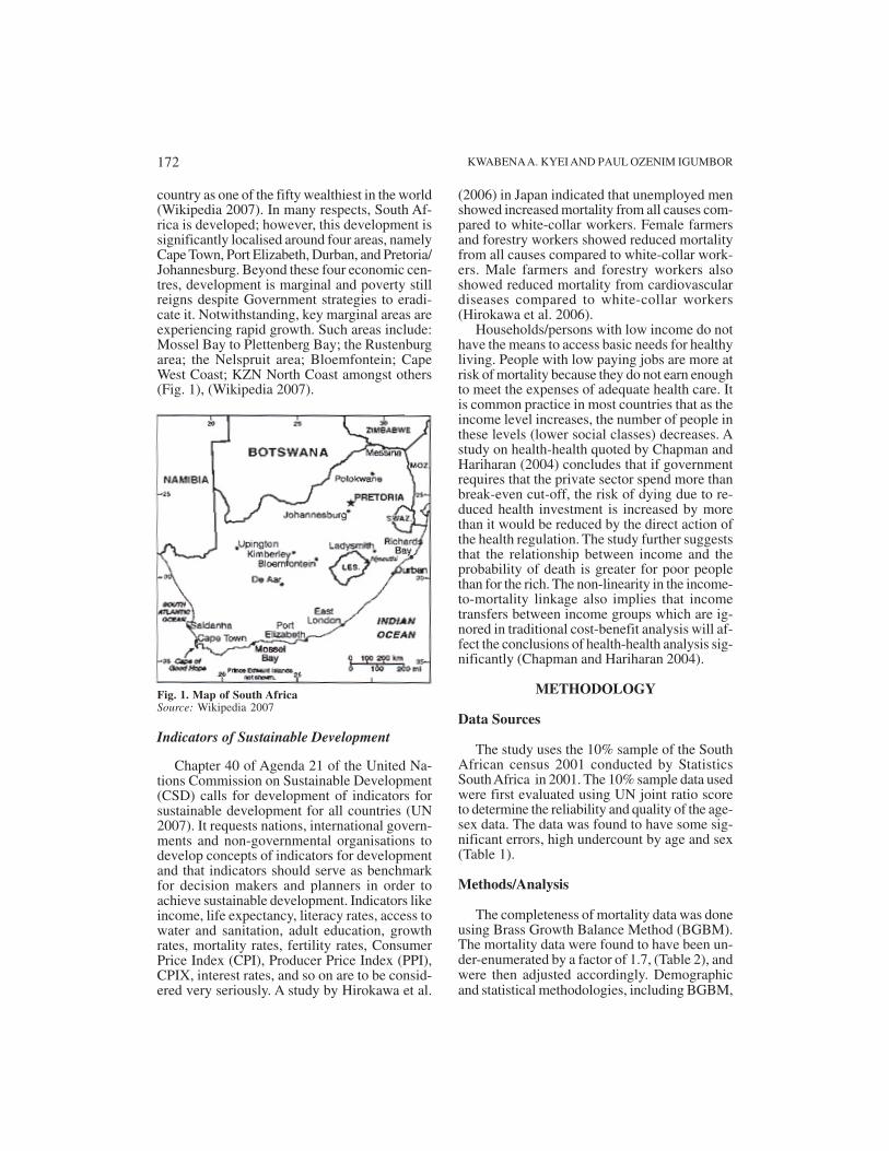
country as one of the fifty wealthiest in the world(Wikipedia 2007). In many respects, South Af-rica is developed; however, this development issignificantly localised around four areas, namelyCape Town, Port Elizabeth, Durban, and Pretoria/Johannesburg. Beyond these four economic cen-tres, development is marginal and poverty stillreigns despite Government strategies to eradi-cate it. Notwithstanding, key marginal areas areexperiencing rapid growth. Such areas include:Mossel Bay to Plettenberg Bay; the Rustenburgarea; the Nelspruit area; Bloemfontein; CapeWest Coast; KZN North Coast amongst others(Fig. 1), (Wikipedia 2007).

Fig. 1. Map of South AfricaSource: Wikipedia 2007

Indicators of Sustainable Development

Chapter 40 of Agenda 21 of the United Na-tions Commission on Sustainable Development(CSD) calls for development of indicators forsustainable development for all countries (UN2007). It requests nations, international govern-ments and non-governmental organisations todevelop concepts of indicators for developmentand that indicators should serve as benchmarkfor decision makers and planners in order toachieve sustainable development. Indicators likeincome, life expectancy, literacy rates, access towater and sanitation, adult education, growthrates, mortality rates, fertility rates, ConsumerPrice Index (CPI), Producer Price Index (PPI),CPIX, interest rates, and so on are to be consid-ered very seriously. A study by Hirokawa et al.

(2006) in Japan indicated that unemployed menshowed increased mortality from all causes com-pared to white-collar workers. Female farmersand forestry workers showed reduced mortalityfrom all causes compared to white-collar work-ers. Male farmers and forestry workers alsoshowed reduced mortality from cardiovasculardiseases compared to white-collar workers(Hirokawa et al. 2006).

Households/persons with low income do nothave the means to access basic needs for healthyliving. People with low paying jobs are more atrisk of mortality because they do not earn enoughto meet the expenses of adequate health care. Itis common practice in most countries that as theincome level increases, the number of people inthese levels (lower social classes) decreases. Astudy on health-health quoted by Chapman andHariharan (2004) concludes that if governmentrequires that the private sector spend more thanbreak-even cut-off, the risk of dying due to re-duced health investment is increased by morethan it would be reduced by the direct action ofthe health regulation. The study further suggeststhat the relationship between income and theprobability of death is greater for poor peoplethan for the rich. The non-linearity in the income-to-mortality linkage also implies that incometransfers between income groups which are ig-nored in traditional cost-benefit analysis will af-fect the conclusions of health-health analysis sig-nificantly (Chapman and Hariharan 2004).

METHODOLOGY

Data Sources

The study uses the 10% sample of the SouthAfrican census 2001 conducted by StatisticsSouth Africa in 2001. The 10% sample data usedwere first evaluated using UN joint ratio scoreto determine the reliability and quality of the age-sex data. The data was found to have some sig-nificant errors, high undercount by age and sex(Table 1).

Methods/Analysis

The completeness of mortality data was doneusing Brass Growth Balance Method (BGBM).The mortality data were found to have been un-der-enumerated by a factor of 1.7, (Table 2), andwere then adjusted accordingly. Demographicand statistical methodologies, including BGBM,

KWABENA A. KYEI AND PAUL OZENIM IGUMBOR172

Table 1: UN method of evaluating age-sex data

Age Sexes Percentages Sex ratio Age ratio Sex ratiogroup deviations % deviations

Xi – X

i+1%

Male Female Male Female Male Female

0-4 185765 186206 99.8 5-9 204605 205236 102.8 102.2 99.7 2.8 2.2 0.110-14 212378 215605 103.3 103.1 98.5 3.3 3.1 1.215-19 206731 213138 108.7 107.8 97.0 8.7 7.8 1.520-24 168068 179922 94.3 94.8 93.4 5.7 5.2 3.625-29 149761 166246 101.2 102.6 90.1 1.2 2.6 3.330-34 127846 144189 96.4 95.5 88.7 3.6 4.5 1.435-39 115354 135577 101.8 104.9 85.1 1.8 4.9 3.640-44 98814 114189 101.3 98.8 86.5 1.3 1.2 1.545-49 79813 95563 98.1 101.6 83.5 1.9 1.6 3.050-54 63842 73949 101.8 98.0 86.3 1.8 2.0 2.855-59 45666 55316 90.4 87.0 82.6 9.6 13.0 3.860-64 37158 53219 103.9 109.6 69.8 8.9 9.6 12.765-69 25843 41800 91.1 95.4 61.8 8.870-74 19555 34436 56.8 Score 4.4 4.9 3.9Joint Score 21.0

Source: 10% Sample size of StatsSA, Census 2001

life table construction and modelling have beensystematically employed.

Brass Growth Balance Method (BGBM)

This is an indirect method of estimating adultmortality. The method is based on the premise

NB: Codes for income

1 = No income 5= R1601 –R3200/month 9=R25601- R51200/month2 = R 1 – R400/month 6=R3201 – R6400/month 10=R51201-R102400/month3 = R401 – R800/month 7=R6401 – R12800/month 11=R102401– R204800/month4 = R801 – R1600/month 8=R12801- R25600/month 12=R204801 or more/month

Codes for school attendance

1 = No 5=Tertiary, Technikon2 = Pre– school 6= University3 =Regular school, (Grade1 10=Adult education to Grade12)4 = College, post-Grade 12 11 = others

Table 2: Brass method for evaluating the quality of mortality data - females

Age group Reported female Population Cumulated Ratiosx-x+4 exact age

(x)N(x)Population Deaths PopulationN(x+) DeathsD(x+) N(x)/N(x+) D(x+)/N(x+)

0-4 186206 2449 1960687 17005 5-9 205236 241 39144.2 1774481 14556 0.022 0.00810-14 215605 181 42084.1 1569245 14315 0.027 0.00915-19 213138 427 42874.3 1353640 14134 0.032 0.01020-24 179922 1040 39306 1140502 13707 0.034 0.01225-29 166246 1637 34616.8 960580 12667 0.036 0.01330-34 144189 1550 31043.5 794334 11030 0.039 0.01435-39 135577 1325 27976.6 650145 9480 0.043 0.01540-44 114189 1065 24976.6 514568 8155 0.049 0.01645-49 95563 890 20975.2 400379 7090 0.052 0.01850-54 73949 727 16951.2 304816 6200 0.056 0.02055-59 55316 575 12926.5 230867 5473 0.056 0.02460-64 53219 797 10853.5 175551 4898 0.062 0.02865-69 41800 802 9501.9 122332 4101 0.078 0.03470-74 34436 909 7623.6 80532 3299 0.095 0.04175+ 46096 2390 46096 2390


MORTALITY LEVEL IN THE NEW SOUTH AFRICA 173

that given a closed population where the infor-mation on age and death distribution have beencorrectly recorded, the number of people at aparticular age can be expressed as a function ofthe growth rate at a particular age and over, thepopulation at that particular age and the numberof deaths of people of the given age. “[It is truethat South Africa is not a closed population, es-pecially after the new dispensation came intoeffect in 1994, many other African nationals havemade South Africa their “home”; and it is equallynoted above that there were errors in the data,and therefore the underlining assumptions ofBGBM are not met. It is however believed thatthe method would still be able to give some cluesas to the growth rate and the quality of the mor-tality data.] “

In mathematical notation, BGBM formula isgiven as,N(x) = r(x+)* N(x+) + D(x+)

where,N(x) = number of people aged xr(x+) = rate of growth aged x and overN(x+) = population aged x and overD(x+) = deaths in population aged x and over

From this, Brass developed an equation of astraight line using these variables such that theintercept on the vertical axis at the origin is therate of growth and the slope is the reciprocal ofthe completeness of death registration. The co-efficients of the equation can then be estimatedusing a number of techniques. The equation forBGBM method can be given asN(x)/N(x+) = r + (1/C)* (D’(x+)/N(x+))

Table 3: Life table for females, South Africa, 2001

Interval nMx nQx L(x) nDx nLx T(x) e(x)

0 0.0702 0.0669 100000 6690 95317.0 5254841.7 52.51—4 0.0099 0.0390 93310 3638 364508.4 5159524.6 55.35—9 0.0020 0.0099 89672 891 446132.4 4795016.2 53.510—14 0.0014 0.0071 88781 631 442327.8 4348883.8 49.015—19 0.0034 0.0169 88150 1488 437028.6 3906556.0 44.320—24 0.0098 0.0480 86662 4156 422918.0 3469527.4 40.025—29 0.0167 0.0803 82506 6628 395958.0 3046609.4 36.930—34 0.0183 0.0874 75878 6630 362811.9 2650651.3 34.935—39 0.0166 0.0798 69247 5523 332428.7 2287839.4 33.040—44 0.0159 0.0763 63724 4859 306473.1 1955410.7 30.745—49 0.0158 0.0761 58865 4482 283118.9 1648937.6 28.050—54 0.0167 0.0802 54383 4362 261007.2 1365818.8 25.155—59 0.0177 0.0846 50020 4233 239520.2 1104811.5 22.160—64 0.0255 0.1197 45788 5480 215239.3 865291.3 18.965—69 0.0326 0.1508 40308 6078 186344.8 650052.0 16.170—74 0.0449 0.2017 34230 6906 153885.8 463707.2 13.575—79 0.0573 0.2506 27324 6847 119503.4 309821.5 11.380—84 0.0764 0.3206 20477 6564 85973.9 190318.1 9.385+ 0.1691 0.5942 13913 8267 104344.2 104344.2 7.5


where,D’(x+) = reported number of deaths of peopleaged x years and over1/C = degree of completeness of deaths recorded

This can simply be expressed as an equationof a straight line; W = a + b*V, where N(x)/N(x+)= W; and (D’(x+)/N(x+) = V with a equals to rand b equals to 1/C, (ECA 1989: 64 - 70).

RESULTS AND DISCUSSION

Tables 3, 4 and 5 present summaries of re-sults obtained. The expectation of life at birthfor male population is 49.8 years and that of thefemale population is 52.5 years. The probabilityof a new-born dying in the first year (denoted by

1q

0) is 0.069 for boys and 0.067 for girls, and the

probability for the same new-born dying in thefirst five years referred to as under-five mortal-ity, denoted by

5q

0 is 0.102 for boys and 0.103

for girls.The proportion of males in the total popula-

tion is 47% and that of females is 53% resultingin a sex ratio of 90. The household size is foundto be 4 and can be considered as comprising about1.9 males and 2.1 females. The distribution byage suggests that the 4 persons per householdconsists of 1.3 persons below 15 years, 0.2 above65 years and 2.5 persons between ages 15 and65. This implies that households are composedof children and members of the economicallyactive age group. Thus most households are likelyto be composed of the nuclear family system,parent(s) and own children only.


Table 5: Life table for combined sexes: South Africa, 2001

Interval nMx nQx l(x) nDx nLx T(x) e(x)

0 0.0716 0.0682 100000.0 6821.6 95224.9 5106278.8 51.061—4 0.0097 0.0380 93178.4 3543.3 364209.6 5011053.9 53.785—9 0.0020 0.0100 89635.1 895.5 445936.5 4646844.3 51.8410—14 0.0015 0.0074 88739.5 658.0 442052.7 4200907.7 47.3415—19 0.0033 0.0162 88081.5 1425.6 436843.8 3758855.0 42.6720—24 0.0088 0.0429 86656.0 3714.7 423992.9 3322011.2 38.3425—29 0.0151 0.0730 82941.2 6052.2 399575.7 2898018.3 34.9430—34 0.0180 0.0859 76889.0 6607.7 367925.9 2498442.7 32.4935—39 0.0181 0.0867 70281.3 6094.6 336170.0 2130516.8 30.3140—44 0.0176 0.0842 64186.7 5406.9 307416.3 1794346.8 27.9645—49 0.0194 0.0924 58779.8 5430.7 280322.1 1486930.5 25.3050—54 0.0219 0.1039 53349.0 5544.3 252884.5 1206608.4 22.6255—59 0.0247 0.1164 47804.8 5563.1 225116.0 953723.9 19.9560—64 0.0325 0.1501 42241.6 6342.3 195352.5 728607.9 17.2565—69 0.0398 0.1811 35899.4 6501.2 163243.8 533255.3 14.8570—74 0.0534 0.2355 29398.2 6924.6 129679.3 370011.5 12.5975—79 0.0672 0.2878 22473.6 6468.4 96196.7 240332.2 10.6980—84 0.0847 0.3494 16005.1 5592.9 66043.5 144135.5 9.0185+ 0.1735 0.6051 10412.3 6300.6 78092.0 78092.0 7.50


Table 4: Life table for males, South Africa, 2001

Interval nMx nQx l(x) nDx nLx T(x) e(x)

0 0.0716 0.0682 100000.0 6818.3 95227.2 4975604.5 49.761—4 0.0093 0.0366 93181.7 3407.7 364548.4 4880377.3 52.375—9 0.0020 0.0100 89774.0 893.3 446636.8 4515828.9 50.3010—14 0.0015 0.0075 88880.7 664.1 442743.4 4069192.1 45.7815—19 0.0031 0.0154 88216.6 1356.8 437691.0 3626448.7 41.1120—24 0.0077 0.0378 86859.8 3280.9 426096.5 3188757.8 36.7125—29 0.0135 0.0653 83578.8 5457.4 404250.7 2762661.3 33.0530—34 0.0175 0.0838 78121.4 6549.1 374234.5 2358410.6 30.1935—39 0.0195 0.0930 71572.3 6653.9 341226.9 1984176.1 27.7240—44 0.0191 0.0911 64918.4 5917.2 309799.2 1642949.2 25.3145—49 0.0228 0.1079 59001.3 6363.4 279097.7 1333150.1 22.6050—54 0.0268 0.1256 52637.8 6610.6 246662.7 1054052.4 20.0255—59 0.0317 0.1469 46027.3 6759.6 213237.3 807389.7 17.5460—64 0.0412 0.1868 39267.6 7333.8 178003.8 594152.4 15.1365—69 0.0507 0.2250 31933.9 7184.6 141707.9 416148.6 13.0370—74 0.0680 0.2906 24749.3 7192.1 105766.2 274440.6 11.0975—79 0.0840 0.3471 17557.2 6094.2 72550.4 168674.4 9.6180—84 0.1036 0.4114 11463.0 4716.3 45524.1 96124.1 8.3985+ 0.1990 0.6644 6746.7 4482.8 50600.0 50600.0 7.50 4975604.5


Table 6 shows the distribution of income bysex. As it is usually the case, males have higherincome than female counterparts. But femaleshave higher expectation of life than males (asseen in Tables 3 and 4). This suggests thereforethat at the individual level, the income level ofthe sexes is not a determinant of mortality rate.The causes of higher mortality rates among malesover females cannot be attributed to the level ofincome which they earn, therefore income couldnot be a predictive factor of mortality at the in-

dividual level. But income could affect mortal-ity at the household level because at that level itis the size of that household that matters.

If the national income is used to provide healthand social services that the people can access,then that can bring about decline in morbidityand mortality. A country with a good social ser-vice scheme would most likely show a smallerrelationship between income and mortality, thana country with a poor social service scheme. Acomparison between Canada and the United


Table 6: Distribution of income by sex

Income Gender Total

Male Female

1 66.5% 70.8% 68.7%2 4.9% 6.0% 5.5%3 8.2% 11.1% 9.8%4 6.7% 4.1% 5.3%5 5.9% 3.4% 4.6%6 3.8% 2.9% 3.3%7 2.3% 1.2% 1.7%8 1.0% .3% 0.7%9 0.4% .1% 0.2%10 0.1% .1% 0.1%11 0.1% .1% 0.1%

Total 100.0% 100.0% 100.0%


States by Ross et al. (2000) concluded thatCanada seemed to counter the increasingly notedassociation at the societal level between incomeinequality and mortality. The lack of a signifi-cant association between income inequality andmortality in Canada may, according to the au-thors, indicate that the effects of income inequal-ity on health are not automatic and may beblunted by the different ways in which social andeconomic resources are distributed in Canada andin the United States (Ross et al. 2000).

Figures 4 and 5 show the proportion of therespondents who were attending school duringthe interview. Figure 2 shows that the level ofeducation for respondents who have attained

Fig. 2. Level of educationSource: 10% Sample size of StatsSA, Census 2001

Fig. 3. Present school attendance by sexSource: StatsSA, 10% sample of the Census 2001[Please note that the proportions for Yes for Male andFemale add to 100%. So are the proportion for No for Maleand Female add up to 100%.]

Fig. 4. Level of education by sexSource: StatsSA, 10% sample of the Census 2001

higher level than grade 12 (twelve years success-ful completion) was at most 5%. Table 7 and Fig-ure 3 show that 65.7% of the respondents agedmore than 5 years were not attending school atthe time of the exercise. Though this proportionincludes those who had graduated from differ-ent levels of schooling, Figure 4 shows that thepercentage of those who have completed highereducation are not more than 5% for any of the


Fig. 5. Employment status by sexSource: StatsSA, 10% sample of the Census 2001

Table 7: Present school attendance

School attendance Frequency Percent

1 2448904 65.72 94085 2.53 1103785 29.64 23138 .65 17442 .56 26514 .710 6565 .211 5222 .1

Total 3725655 100.0


A study by Zajacova (2006) showed that inthe US, education had a comparable effect onmortality for men and women. No statisticallysignificant gender difference was found in all-cause mortality or mortality by cause of death,among younger persons, and among the elderly.Analysis by marital status, however, suggestedthat these findings apply only to married menand women. Among the divorced, there was astatistically significant sex difference wherebyeducation had effect on mortality for women butnot on men (Zajacova 2006). That is proven by astrong education gradient (seven percent lowerodds of dying for each year of schooling).

A similar study by Hurt et al. (2004) based ondata from Bangladesh showed that mortality waslower in women with formal or Koranic educa-tion compared with those with none. After ad-justing for her own education, the husband’s levelof education or occupation did not have an inde-pendent effect on a woman’s survival. Men whohad attended formal education had lower mor-tality than those without any education, but menwhose wives had been educated had an additionalsurvival advantage independent of their own edu-cation and occupation. Mortality in both sexeswas also significantly associated with marital sta-tus and the percentage of surviving children andin men mortality was associated with the man’soccupation, religion and area of residence.

In Japan, early termination of education wasassociated with an increased risk of mortalityfrom all causes of death for both men and women.For men specifically, cardiovascular diseasemortality for all men was increased by early ter-mination of education compared to later termi-nation (Hirokawa et al. 2006).

The effect of income-mortality based on sexhas been one of contentious issues in most de-veloped countries. According to Backlund et al.(2007), some of the most consistent evidence infavour of an association between income inequal-ity and health has been among the US states. Theresearchers concluded that the relationship be-tween income inequality and mortality is onlyrobust to adjustment for compositional factorsin men and women under 65, and that certaincauses of death that occur primarily in the popu-lation under 65 may be associated with incomeinequality. They also noted that this result ex-plains why income inequality is not a major driverof mortality trends in the US because most deathsoccur at ages 65 and over.

They further concluded that certain causes ofdeath that occur primarily in the population un-der 65 may be associated with income inequal-ity. In the Limpopo province in South Africa,Kyei and Gyekye (2012) have showed that theproportion of the unemployed female populationfar exceeds the proportion of the males. Thisclearly suggests that employment cannot be thereason for the differences in mortality rates be-tween males and females. There should be someother reasons (possibly the physiological make-up of the sexes) that make males to have highermortality than females.

According to Guttmacher Institute (2002), onthe average, 61 babies die for every 1000 live


sexes. Education is very important, especiallywhen we consider women’s education where ithas been found that female education above grade12 has a negative effect on childhood mortality(Kyei 1995). The effect that mother’s educationhas on childhood mortality is far higher than theeffect that father’s education has on mortality).

births in developing countries, compared witheight deaths per 1000 in developed countries. Insome developing countries, the rates are muchhigher than the average. For example, in Sub-Saharan Africa—the world’s poorest region—more than one in 10 infants die (that is, 100 per1000) before age one in Benin, Burkina Faso,Central African Republic, Chad, Ethiopia,Guinea, Malawi, Mali, Mozambique, Niger, Tan-zania and Zambia. Per capita income is below$2000 in all of these countries; in many, it is$500-900 (Blacklund et al. 1996). In countrieswhere per capital income is higher, infant mor-tality rates are substantially lower. High infantmortality is, therefore, clearly a result of pov-erty, which creates conditions—for example, thelack of clean water, poor sanitation, malnutrition,endemic infections, poor or nonexistent primaryhealth care services and low levels of spendingon health care—in which babies who are not ro-bust at birth do not receive the health care theyneed to overcome their vulnerability (GuttmacherInstitute 2002). A reduction in the levels of in-fant mortality can therefore be averted by animprovement in the per capita income of parentsand guardians.

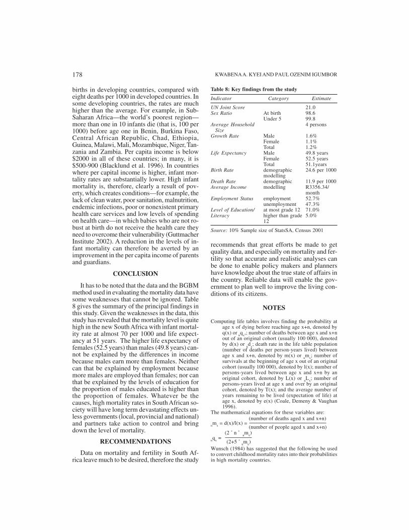
CONCLUSION

It has to be noted that the data and the BGBMmethod used in evaluating the mortality data havesome weaknesses that cannot be ignored. Table8 gives the summary of the principal findings inthis study. Given the weaknesses in the data, thisstudy has revealed that the mortality level is quitehigh in the new South Africa with infant mortal-ity rate at almost 70 per 1000 and life expect-ancy at 51 years. The higher life expectancy offemales (52.5 years) than males (49.8 years) can-not be explained by the differences in incomebecause males earn more than females. Neithercan that be explained by employment becausemore males are employed than females; nor canthat be explained by the levels of education forthe proportion of males educated is higher thanthe proportion of females. Whatever be thecauses, high mortality rates in South African so-ciety will have long term devastating effects un-less governments (local, provincial and national)and partners take action to control and bringdown the level of mortality.

RECOMMENDATIONS

Data on mortality and fertility in South Af-rica leave much to be desired, therefore the study

Table 8: Key findings from the study

Indicator Category Estimate

UN Joint Score 21.0Sex Ratio At birth 98.6 Under 5 99.8Average Household 4 persons SizeGrowth Rate Male 1.6% Female 1.1% Total 1.2%Life Expectancy Male 49.8 years Female 52.5 years Total 51.1yearsBirth Rate demographic 24.6 per 1000

modellingDeath Rate demographic 11.9 per 1000Average Income modelling R3356.34/

monthEmployment Status employment 52.7% unemployment 47.3%Level of Education/ at most grade 12 71.0%Literacy higher than grade 5.0%

12


recommends that great efforts be made to getquality data, and especially on mortality and fer-tility so that accurate and realistic analyses canbe done to enable policy makers and plannershave knowledge about the true state of affairs inthe country. Reliable data will enable the gov-ernment to plan well to improve the living con-ditions of its citizens.

NOTES

Computing life tables involves finding the probability atage x of dying before reaching age x+n, denoted byq(x) or

nq

x,; number of deaths between age x and x+n

out of an original cohort (usually 100 000), denotedby d(x) or

nd

x; death rate in the life table population

(number of deaths per person-years lived) betweenage x and x+n, denoted by m(x) or

nm

x; number of

survivals at the beginning of age x out of an originalcohort (usually 100 000), denoted by l(x); number ofpersons-years lived between age x and x+n by anoriginal cohort, denoted by L(x) or

nL

x; number of

persons-years lived at age x and over by an originalcohort, denoted by T(x); and the average number ofyears remaining to be lived (expectation of life) atage x, denoted by e(x) (Coale, Demeny & Vaughan1996).

The mathematical equations for these variables are:(number of deaths aged x and x+n)

(number of people aged x and x+n)nm

x = d(x)/l(x) =

(2 * n * nm

x)

nq

x =

(2+5 * nm

x)

Wunsch (1984) has suggested that the following be usedto convert childhood mortality rates into their probabilitiesin high mortality countries.


For people aged 0 to 1, this is given as 1q

0 = (2 *

nm

x) /

(2+1.4* nm

x)

For people aged 1 to 4, this is given as 1q

4 = (2 * 4 *

nm

x) /

(2+3.7 * nm

x)

Lx = (n/2) * (l(x) + l(x+n)) assumed linear relationship

between age x and x+nAgain Wunsch (1984) recommends that the childhoodpersons-year be calculated as follows:For people age 0 to 1, this is given as

1L

0 = 0.3*l

0 + 0.7* l

0

For people age 1 to 4, this is given as 4L

1 = 1.6*l

1 + 2.4* l

4

T(x) = Σ nL

x and e(x) = T(x) / l(x)

REFERENCES

Backlund E, Sorlie PD, Johnson NJ 1996. The shape of therelationship between income and mortality in theUnited States – Evidence from the national longitudinalmortality studies. Annals of Epidemiology, 6(1): 12-20.

Backlund E, Rowe G, Lynch J, Wolfson MC, Kaplan GA,Sorlie PD 2007. Income inequality and mortality: Amultilevel prospective study of 521 248 individuals in50 US states. US Bureau of the Census, Washington,DC20233, USA. International Journal of Epidemio-logy, 36(3): 590–596.

Chapman KS, Hariharan G 2004. Do poor people have astronger relationship between income and mortalitythan the rich? Implications of panel data for health-health analysis. Journal of Risk and Uncertainty, 12(1):51–63.

CIA 2007. World Fact Book. From <http://cia.gov/library/publications/the-world-factbook.>

Coale A, Demeny P, Vaughan B 1996. Regional Model LifeTables and Stable Populations. 2nd Edition. NewJersey: USA, Academic Press.

Dorrington R, Moultrie TA, Timeaus IM 2004. Estimationof Mortality Using the South African Census 2001Data. Centre for Actuarial Research (CARe)Monograph 11. UCT: Cape Town.

Duleep H 1995. Mortality and income inequality amongeconomically developed countries. Social SecurityBulletin, Summer 1995.

ECA 1989. Workbook on Demographic Data Evaluationand Analysis. RIPS: Accra.

Guttmacher Institute 2002. Family Planning Can reduceHigh Infant Mortality rate. Issues in Brief.

Hirokawa K, Tsutusmi A, Kayaba K 2006. Impacts ofeducational level and employment status on mortalityfor Japanese women and men: The Jichi MedicalSchool cohort study. European Journal of Epidemio-logy, 21(9): 641-51.

Hurt LS, Ronsmans C, Saha S 2004. Effects of Educationand Other Socio-economic Factors on Middle AgeMortality in Rural Bangladesh. UK: Maternal HealthProgramme, Department of Infectious and TropicalDiseases London School of Hygiene and TropicalMedicine, London.

Kyei KA 1995. Childhood Mortality in South Africa:Factors Affecting the Intensity and Trend. Ph. D.Thesis, Unpublished. Pretoria: University of Pretoria.

Kyei KA 2011. Socio-Economic factors affecting under-fivemortality in South Africa – An investigative study.JETEMS 2(2): 104 - 110.

Kyei KA 2012. Determinants of childhood mortality in SouthAfrica: Using categorical data modelling. J Hum Ecol,37(1): 47 - 56.

Kyei KA, Gyekye KB 2012. Unemployment in LimpopoProvince in South Africa: Searching for factors. J SocSci, 31(2): 177 - 185.

Ross NA, Wolfson MC, Dunn JR, Berthelot J, Kaplan GA,Lynch JW 2000. Relation between income inequalityand mortality in Canada and in the United States:Cross- Sectional Assessment Using Census Data andVital Statistics. British Medical Journal, 2000: 1:320(7239): 898–902.

United Nations 2007. Indicators of Sustainable Develop-ment. United Nations Commission for SustainableDevelopment. New York: UN.

Wikipedia, South Africa 2007.Wunsch G 1984. Techniques d’analyse des donnees

demographiques dificientes. Liege: Ordina Editions.Zajacova A 2006. Education, gender, and mortality: Does

schooling have the same effect on mortality for menand women in the US, Office of the populationresearch, Princeton University.


mortality level in the new south africa: looking for … level in the new south africa: looking for...

Documents