Mortgage Design in an Equilibrium Model of the Housing Market

Adam M. Guren∗, Arvind Krishnamurthy†, and Timothy J. McQuade‡§

May 29, 2018

First Version: March 20, 2017

Abstract

How can mortgages be redesigned to reduce housing market volatility, consumption volatility,

and default? How does mortgage design interact with monetary policy? We answer these

questions using a quantitative equilibrium life cycle model with aggregate shocks, long-term

mortgages, and an equilibrium housing market, focusing on designs that index payments to

monetary policy. Designs that raise mortgage payments in booms and lower them in recessions

do better than designs with fixed mortgage payments. The welfare benefits are quantitatively

substantial: ARMs improve household welfare relative to FRMs by the equivalent of 0.83 percent

of annual consumption under a monetary regime in which the central bank lowers real interest

rates in a bust. Among designs that reduce payments in a bust, we show that those that

front-load the payment reductions and concentrate them in recessions outperform designs that

spread payment reductions over the life of the mortgage. Front-loading alleviates household

liquidity constraints in states where they are most binding, reducing default and stimulating

housing demand by new homeowners. To isolate this channel, we compare an FRM with a

built-in option to be converted to an ARM with an FRM with an option to be refinanced

at the prevailing FRM rate. Under these two contracts, the present value of a lender’s loan

falls by roughly an equal amount, as these contracts primarily differ in the timing of expected

repayments. The FRM that can be converted to an ARM, which front loads payment reductions,

improves household welfare by four times as much.

∗Boston University, guren@bu.edu†Stanford University Graduate School of Business and NBER, a-krishnamurthy@stanford.edu‡Stanford University Graduate School of Business, tmcquade@stanford.edu§The authors would like to thank Chaojun Wang and Xuiyi Song for excellent research assistance and seminar

participants at SED, SITE, Kellogg, Queen’s, Indiana, LSE, Boston University, HULM, Housing: Micro Data, MacroProblems, NBER Summer Institute Capital Markets and the Economy, CEPR Housing and the Macroeconomy,Chicago Booth Asset Pricing, UCLA, University of Pittsburgh, MIT Sloan, Wharton, the University of Pennsylvania,Tomasz Piskorski, Erwan Quintin, Jan Eberly, Alex Michaelides, Alexei Tchistyi, and Andreas Fuster for usefulcomments. Guren acknowledges research support from the National Science Foundation under grant #1623801 andfrom the Boston University Center for Finance, Law, and Policy.

1 Introduction

The design of mortgages is crucial to both household welfare and the macroeconomy. Home equity

is the largest component of wealth for most households, and mortgages tend to be their dominant

source of credit, so the design of mortgages has an outsized effect on household balance sheets

(Campbell, 2013). In the mid-2000s boom and subsequent bust, housing wealth extraction through

the mortgage market boosted consumption in the boom and reduced consumption in the bust (e.g.,

Mian and Sufi, 2011; Mian, Rao, and Sufi, 2013). Mortgage debt also led to the wave of foreclosures

that resulted in over six million households losing their homes, badly damaging household balance

sheets and crippling the housing market (e.g., Guren and McQuade, 2018; Mian, Sufi, and Trebbi,

2015). Finally, in the wake of the recession, there has been increased attention paid to the role

that mortgages play in the transmission of monetary policy to the real economy through household

balance sheets (e.g., Auclert, 2017; Wong, 2018; Di Maggio et al., 2017; Beraja et al., 2017).

In this paper, we study how to best design mortgages in order to reduce household consumption

volatility and default and to increase household welfare. There is considerable evidence that im-

plementation frictions prevent financial intermediaries from modifying mortgages ex post in a crisis

(e.g., Agarwal et al., 2015; Agarwal et al., 2017). As a result, a better-designed ex ante contract can

likely deliver significant welfare benefits (e.g., Campbell and Cocco, 2015; Piskorski and Tchistyi,

2017; Greenwald, Landvoigt, and Van Nieuwerburgh, 2018; Piskorski and Seru, 2018). We are

further motivated by the evidence that not just the level of household mortgage debt (e.g., loan-to-

value or payment-to-income ratio), but also the design of such debt, can impact household outcomes

including consumption and default. For example, Fuster and Willen (2017) and Di Maggio et al.

(2017) study cohorts of borrowers with hybrid adjustable rate mortgages contracted in the years

before the crisis. Exploiting heterogeneity in the timing of monthly payment reductions as mort-

gages transitioned from initial fixed rates to adjustable rates during the crisis, these papers show

that downward resets resulted in substantially lower defaults and increased consumption. Similarly,

studies that exploit quasi-random variation in housing market interventions in the Great Recession

such as the Home Affordable Refinance Program (HARP) (Agarwal et al., 2017) and the Home

Affordable Modification Program (HAMP) (Agarwal et al., 2017; Ganong and Noel, 2017) have

found that monthly payment reductions significantly reduced default and increased consumption.

Such empirical evidence suggests that given the cyclicality of interest rates, indexing mortgage

payments to interest rates can improve household outcomes and welfare. We pursue this indexation

question systematically using a quantitative equilibrium model featuring heterogeneous households,

endogenous mortgage spreads, and endogenous house prices. In a crisis, default increases the supply

of homes on the market, further pushing down prices, which in turn generates more default. Using

this framework, we quantitatively assess a variety of questions related to mortgage design. How

would consumption, default, home prices, and household welfare change if we were to alter the

design of mortgages in the economy, particularly in a deep recession and housing bust like the one

experienced during the Great Recession? In an economy that transits between booms, recessions,

and crises, how well do different indexed mortgages perform? What is the most effective simple

form of indexation?

Designs in which mortgage payments are higher in booms and lower in recessions do better than

1

designs with fixed mortgage payments for risk and insurance reasons. But among such designs the

most effective ones front-load the payment reductions so that they are concentrated during reces-

sions rather than spread out over the life of the mortgage. Front-loading payment relief smooths

consumption and limits default for homeowners who are liquidity constrained and stimulates hous-

ing demand by constrained renters. The reduction in default and increase in demand helps short-

circuit a price-default spiral. Consequently, the benefit of different designs depends largely on how

effectively they deliver immediate payment reductions to highly constrained households.

Our model features overlapping generations of households subject to both idiosyncratic and

aggregate shocks, making endogenous decisions over home purchases, borrowing, consumption,

refinancing, and costly default. We consider different relationships between the interest rate and the

exogenous aggregate state, reflecting alternative monetary policies. Competitive and risk-neutral

lenders set spreads for each mortgage to break even in equilibrium, so lenders charge higher interest

rates when a mortgage design hurts their bottom line. Equilibrium in the housing market implies

that household decisions, mortgage spreads, and the interest rate rule influence the equilibrium

home price process. Household expectations regarding equilibrium prices and mortgage rates feed

back into household decisions, and we solve this fixed-point problem in a rich quantitative model

using computational methods based on Krusell and Smith (1998).

A key aspect of our analysis is that mortgage design affects household default decisions and

hence home prices, which in equilibrium feeds back to household indebtedness. The quantitative

implications of our model depend on accurately representing the link between home prices and

default. Consequently, after calibrating our model to match standard moments, monetary policy

since the 1980s, and the empirical distributions of mortgage debt and assets, we evaluate its ability

to quantitatively capture the effect of payment reductions on default by simulating the Fuster and

Willen (2017) quasi-experiment in our model. The model does a good job matching their findings

quantitatively. Simulating quasi-experiments in our calibration procedure is an innovation that

ensures that our model accurately captures the effects of changes in LTVs and interest rates as we

alter mortgage design.

The calibrated model provides a laboratory to assess the benefits and costs of different mortgage

designs. Our primary application is the impulse response to a housing crisis, although we also

consider the unconditional performance of different mortgages. We begin by comparing an economy

with all fixed rate mortgages (FRMs) against one with all adjustable rate mortgages (ARMs). While

ARMs and FRMs are not necessarily optimal contracts, they provide the simplest and starkest

comparison for us to analyze the benefits of indexation. We find that in a counterfactual economy

suffering a crisis similar to the 2007-2009 recession with all ARMs instead of all FRMs, house prices

fall by 2.7 percentage points less, 26.1 percent fewer households default, consumption falls by 0.8

percentage points less, and the overall welfare impact of a housing crisis is ameliorated by the

equivalent of 0.83 percent of annual consumption. Young, liquidity constrained households benefit

to an even greater extent, with ARMs increasing their welfare by up to four percent of annual

consumption relative to FRMs.

ARMs alleviate the impact of the crisis for three reasons. First, ARMs deliver larger payment

reductions to constrained homeowners due to front-loading. ARM rates fall significantly more than

2

FRM rates during the crisis because FRM rates are determined by the long end of the yield curve,

which falls by less due to the logic of the expectations hypothesis. With FRMs, the payment

relief is spread out over the remaining life of the mortgage, but with ARMs it is concentrated in

the crisis. Second, ARMs automatically pass interest rate reductions through to households. By

contrast, FRMs only pass-through rate reductions when households refinance, which is not possible

for households that, due to the fall in house prices, have insufficient equity to satisfy the LTV

constraint. Therefore, underwater homeowners who are most at risk of default and in need of

liquidity relief are unable to receive any. Since ARMs provide greater hedging benefits against

declining labor income during the crisis, there is less default by underwater homeowners which

short-circuits the equilibrium price-default spiral and leads to a less-severe housing crisis. Third

and finally, because ARM rates fall more than FRM rates, ARMs are more effective at stimulating

housing demand by constrained renters in the crisis, which further limits price declines and the

price-default spiral.

One issue with a pure ARM is that in an inflationary episode, real interest rates can spike up

while real income falls, with potentially catastrophic consequences. We consequently consider a

new mortgage design that partially protects from this scenario: a fixed rate mortgage with a one-

time option to convert to an adjustable rate mortgage, as suggested by Eberly and Krishnamurthy

(2014). Of course, borrowers pay for the prepayment option with a higher average loan rate, which

is offset somewhat by banks anticipating fewer defaults and losses in a crisis. Despite this cost, this

“EK convertible” mortgage delivers much better outcomes than a standard fixed rate mortgage:

it realizes 90 percent of the benefits of the all-ARM economy when rates fall in a downturn, but

experiences only 45 percent of the downside in an inflationary episode in which rates rise during a

housing bust.

We also consider a “FRM with an underwater refinancing option” (FRMUR) in which house-

holds with a fixed-rate mortgage have an option to refinance in a crisis into another fixed-rate

mortgage with equal principal regardless of their loan-to-value ratio. This is motivated by the fact

that lower long rates were not passed through to underwater households, which also motivated

the government’s HARP program. While the FRMUR does help these households, it does so by

relatively little because the long end of the yield curve does not fall by much, and so the payment

relief provided by the FRMUR is limited. Indeed, the consumption equivalent welfare gain relative

to FRM for the FRMUR is a quarter of that of the EK convertible mortgage. This is the case

despite the fact that the decline in the present value of the bank’s mortgage portfolio when the crisis

hits is similar under these two designs. Intuitively, because lenders are not liquidity constrained,

they care only about the present value of their portfolio, which, modulo differences in default risk

and prepayment risk, is largely unchanged by trading lower payments in the short run for higher

payments in the future because of an endogenously-holding yield curve.

The comparison of the EK convertible mortgage with the FRM with an option to be refinanced

underwater provides the sharpest example of our central finding that the best designs are those

that deliver immediate payment relief to liquidity constrained households rather than spreading

the relief over the entire term of the mortgage. Consistent with this, we show that an option ARM

design, which allows households to negatively amortize the mortgage up to a cap when liquidity

3

needs arise at a cost of higher payments in the future, delivers welfare benefits superior to both EK

and ARM. Unlike those designs, the option ARM allows borrowers to defer payments as a function

of her idiosyncratic state. Our analysis quantifies the benefits of such insurance in the mortgage

contract, although we do not model the adverse selection it can induce.

Our analysis also calls attention to an important externality: when deciding their personal debt

position, households do not internalize the impact of their debt choice and liquid asset position

on macro fragility. This has important consequences in our model. For instance, ARMs provide

more relief relative to FRMs if they are introduced at the moment the crisis occurs rather than

ex ante. This is the case because homeowners expect the central bank to provide insurance by

reducing short rates in the ARM economy and take on more risk by levering up more and holding

less liquid savings, undoing some of the insurance benefit. Similarly, the insurance benefits of an

option ARM (OARM) design encourage households to take on more leverage risk ex ante, which

creates a more fragile pre-crisis LTV distribution than would otherwise be the case and limits the

welfare benefits of the option ARM, which would be enormous if one were to neglect the change

in the ex ante distribution of households across states. These results highlight that policy makers

must account for the fact that households do not share their macro-prudential concerns and may

take on too much debt from a social planner’s perspective when insurance is offered.

Finally, we find that monetary policy and mortgage design should not be studied in isolation.

Indeed, monetary policy efficacy depends on mortgage design, and mortgage design efficacy de-

pends on monetary policy. We highlight this interaction by considering the performance of various

mortgage designs under alternate monetary policies. We show that mortgage designs tied to the

long rate such as FRM and FRMUR are most effective when combined with unconventional mon-

etary policies, such as the Fed’s quantitative easing (QE) purchases of mortgage-backed securities

to lower long-term mortgage rates. This result also implies that ex-post policies such as HARP

need to be combined with QE policies in order to be maximally effective. Still, FRMUR coupled

with quantitative easing does not improve welfare relative to an ARM or EK mortgage under con-

ventional monetary policy, which suggests that many of the benefits of unconventional monetary

policy for the housing market can be achieved more directly through mortgage design coupled with

conventional monetary policy. This highlights the importance of studying mortgage design and

monetary policy jointly.

The remainder of the paper is structured as follows. Section 2 describes the relationship to the

existing literature. Section 3 presents our model, and Section 4 describes our calibration procedure.

Section 5 compares the performance of ARM-only and FRM-only economies to develop economic

intuition. Section 6 compares more exotic mortgage designs that combine beneficial features of

both FRMs and ARMs, and Section 7 considers the interaction of mortgage design with monetary

policy. Section 8 concludes.

2 Related Literature

This paper is most closely related to papers that analyze the role of mortgages in the macroecon-

omy through the lens of a heterogeneous agents model. In several such papers, house prices are

4

exogenous. Campbell and Cocco (2015) develop a life-cycle model in which households can borrow

using long-term fixed- or adjustable-rate mortgages and face income, house price, inflation, and

interest rate risk. They use their framework to study mortgage choice and the decision to default.

In their model, households can choose to pay down their mortgage, refinance, move, or default,

and mortgage premia are determined in equilibrium through a lender zero-profit condition. Our

modeling of households shares many structural features with this paper, but while they take house

prices as an exogenous process, we crucially allow for aggregate shocks and determine equilibrium

house prices. This critical feature of our model allows us to study the interaction of mortgage

design with endogenous price-default spirals. A prior paper, Campbell and Cocco (2003), use a

more rudimentary model without default and with exogenous prices to compare ARMs and FRMs

and assess which households benefit most from each design. Similarly, Corbae and Quintin (2015)

present a heterogeneous agents model in which mortgages are priced in equilibrium and households

select from a set of mortgages with different payment-to-income requirements, but again take house

prices as exogenous. They use their model to study the role of leverage in triggering the foreclo-

sure crisis, placing particular emphasis on the differential wealth levels and default propensities

of households that enter the housing market when lending standards are relaxed. Conversely, we

focus on the impact of mortgage design and monetary policy on housing downturns, allowing for

endogenous house price responses.

Other heterogeneous agent models of the housing market have endogenous house prices but lack

aggregate shocks or rich mortgage designs. Kung (2015) develops a heterogeneous agents model

of the housing market in which house prices are determined in equilibrium. His model, however,

lacks aggregate shocks and household saving decisions. He focuses specifically on the equilibrium

effects of the disappearance of non-agency mortgages during the crisis. By contrast, we include

aggregate shocks and a rich set of household decisions that Kung assumes away. We also study

a variety of mortgage designs and analyze how mortgage design interacts with monetary policy.

Kaplan, Mitman, and Violante (2017) present a life-cycle model with default, refinancing, and

moving in the presence of idiosyncratic and aggregate shocks in which house prices are determined

in equilibrium. Their focus, however, is on explaining what types of shocks can explain the joint

dynamics of house prices and consumption in the Great Recession. They simplify many features of

the mortgage contract for tractability in order to focus on these issues, while our paper simplifies

the shocks and consumption decision in order to provide a richer analysis of mortgage design.1

Our paper also builds on a largely theoretical literature studying optimal mortgage design.

These papers identify important trade-offs inherent in optimal mortgage design in a partial equi-

librium settings. Concurrent research by Piskorski and Tchistyi (2017) studies mortgage design in

a setting with equilibrium house prices and asymmetric information in a two-period model. The

intuition they develop about the insurance benefits of state contingent contracts is complementary

to our own, which is is more focused on the timing of payments over the life of the loan. Concur-

rent research by Greenwald, Landvoigt, and Van Nieuwerburgh (2017) studies shared appreciation

mortgages (SAMs) that index payments to aggregate house prices in a model with a fragile financial

1For instance, Kaplan, Mitman, and Violante (2017) assume that all mortgages have a single interest rate andthat lenders break even by charging differential up front fees. By contrast, we maintain each borrower’s interest rateand contract choice as a state variable.

5

sector. They show that the losses incurred by banks in a deep recession quantitatively outweigh

the benefits to household balance sheets under a SAM. Our papers are highly complementary: we

highlight the benefits of front-loading payment relief in mortgage designs that shift risk from house-

holds to financial intermediaries to a much more limited degree than a SAM, while GLVN study

whether such risk shifting would be beneficial. Indeed, we have experimented with SAMs in our

framework and found that the losses that banks incur in a crisis are an order of magnitude larger

than in the designs we consider. Piskorski and Tchistyi (2010; 2011) consider mortgage design from

an optimal contracting perspective, finding that the optimal mortgage looks like an option ARM

when interest rates are stochastic and a subprime loan when house prices are stochastic. Brueckner

and Lee (2017) focus on optimal risk sharing in the mortgage market. Our paper is also related to a

literature advocating certain macroprudential polices aimed at ameliorating the severity of housing

crises. Mian and Sufi (2015) advocate for modifications through principal reduction, while Eberly

and Krishnamurthy (2014) advocate for monthly payment reductions. Greenwald (2017) advocates

for payment-to-income constraints as a macroprudential policy to reduce house price volatility.

To calibrate our model, we draw on a set of papers which document empirical facts regarding

household leverage and default behavior. Foote et al. (2008) provide evidence for a “double

trigger” theory of mortgage default, whereby most default is accounted for by a combination of

negative equity and an income shock as is the case in our model. Bhutta et al. (2010), Elul et

al. (2010), and Gerardi et al. (2013) provide further support for illiquidity as the driving source

of household default. Fuster and Willen (2017) and Di Maggio et al. (2017) show that downward

rate resets lead to reductions in default and increases in household consumption, respectively.

Agarwal et al. (2015), Agarwal et al. (2017), and Ganong and Noel (2017) study the HAMP

and HARP programs and find similarly large effects of payment on default and consumption and

limited effects of principal reduction for severely-underwater households, which they relate to the

immediate benefits of payment relief versus the delayed benefits of principal reduction. This micro

evidence motivates our focus on mortgage designs with state-contingent payments, and we use

Fuster and Willen’s evidence to evaluate the quantitative performance of our model.

Finally, our research studies how mortgage design interacts with monetary policy and thus

relates to a literature examining the transmission of monetary policy through the housing market.

Caplin, Freeman, and Tracy (1997) posit that in depressed housing markets where many borrowers

owe more than their house is worth, monetary policy is less potent because individuals cannot

refinance. Beraja, Fuster, Hurst, and Vavra (2017) provide empirical evidence for this hypothesis

by analyzing the impact of monetary policy during the Great Recession. Relatedly, a set of papers

have argued that adjustable-rate mortgages allow for stronger transmission of monetary policy since

rate changes directly affect household balance sheets (Calza et al., 2013; Auclert, 2017; Cloyne et

al., 2017). Garriga et al. (2016) provide a model with long-term debt that features a yield curve

and is related to our findings about the differential effects of mortgage designs that are priced off the

short end relative to the long end of the yield curve. Di Maggio et al. (2017) show empirically that

the pass-through of monetary policy to consumption is stronger in regions with more adjustable

rate mortgages. Finally, Wong (2018) highlights the role that refinancing by young households

plays in the transmission of monetary policy to consumption.

6

3 Model

This section presents an equilibrium model of the housing market that we subsequently use as a

laboratory to study different mortgage designs. Home prices and mortgage spreads are determined

in equilibrium. Short-term interest rates, on the other hand, are exogenous to the model and depend

on the aggregate state of the economy, reflecting an exogenous monetary policy rule. For ease of

exposition, we present the model for the case of an all-FRM economy or an all-ARM economy, but

consider other designs when presenting our quantitative results.

3.1 Setup

Time is discrete and indexed by t. The economy consists of a unit mass of overlapping generations

of heterogeneous households of age a = 1, 2, ..., T who make consumption, housing, borrowing,

refinancing and default decisions over their lifetime. Household decisions depend both on aggregate

state variables Σt and agent-specific state variables sjt , where j indexes agents. Unless otherwise

stated, all variables are agent-specific, and to simplify notation, we suppress their dependency on

sjt .

The driving shock process in the economy is Θt, which is part of Σt. Θt follows a discrete Markov

process over five states Θt ∈Crisis With Tight Credit, Recession With Tight Credit, Recession

With Loose Credit, Expansion With Tight Credit, Expansion With Loose Credit. Θt is governed

by a transition matrix ΞΘ described subsequently.

Each generation lives for T periods. At the beginning of a period, a new generation is born and

shocks are realized. Agents then make decisions, and the housing market clears. Utility is realized

and the final generation dies at the end of the period. Households enter period t with a state sjt−1

and choose next period’s state variables sjt in period t given the period t housing price pt. Utility

is based on period t choices, and the short rate rt realized at time t is the interest rate between t

and t+ 1.

Households receive flow utility from housing Ht and non-durable consumption Ct:2

U (Ct, Ht) =C1−γt

1− γ+ αaHt.

In the last period of life, age T , a household with terminal wealth b receives utility:

C1−γt

1− γ+ ψ

(b+ ξ)1−γ

1− γ,

whereHT = 0 because the terminal generation must sell.3 For simplicity, we assume that households

use their wealth to finance housing and end-of-life care after their terminal period. Consequently,

2The term αa describes the utility from homeownership as a function of age. In our calibration, we will assumethat αa is decreasing in age so as to reflect the fact that at older ages the homeownership rate declines slightly.

3Including terminal wealth in the utility function is standard in OLG models of the housing market becauseotherwise households would consume their housing wealth before death. In the data, however, the elderly havesubstantial housing wealth which they do not consume. The functional form for the utility derived from terminalwealth is standard.

7

the wealth b is not distributed to incoming generations, who begin life with no assets.

Households receive an exogenous income stream Yt:

Yt ≡ exp(yaggt (Θt) + yidt

).

Log income is the sum of an aggregate component that is common across households and a

household-specific idiosyncratic component. The aggregate component yaggt is a function of the

aggregate state Θt. The idiosyncratic component yidt is a discrete Markov process over a setY idt

with transition matrix Ξid (Θt).

Households retire at age R < T . After retirement, households no longer face idiosyncratic

income risk and keep the same idiosyncratic income they had at age R, reduced by ρ log points

to account for the decline in income in retirement. This can be thought of as a social security

benefit that conditions on terminal income rather than average lifetime income for computational

tractability, as in Guvenen and Smith (2014).

There is a progressive tax system so that individuals’ net-of-tax income is Yt − τ (Yt). The tax

system is modeled as in Heathcote et al. (2017) so that:

τ (Yt) = Yt − τ0Y1−τ1t .

Houses in the model are of one size, and agents can either own a house (Ht = 1) or rent a house

(Ht = 0).4 There is a fixed supply of housing and no construction implying that the homeownership

rate is constant.5 Buying a house at time t costs pt, and owners must pay a per-period maintenance

cost of mpt. With probability ζ, homeowners experience a life event that makes them lose their

match with their house and list it for sale, while with probability 1− ζ, owners are able to remain

in their house.

The rental housing stock is entirely separate from the owner-occupied housing stock. Rental

housing can be produced and destroyed at a variable cost q, so in equilibrium renting costs q per

period. Although this assumption is stark, it is meant to capture that while there is some limited

conversion of owner-occupied homes to rental homes and vice-versa in practice, the rental and

owner-occupied markets are quite segmented (Glaeser and Gyourko, 2009; Halket et al., 2015).

This assumption implies that movements in house prices are accompanied by movements in the

price-to-rent ratio. Indeed, in the data, the price-to-rent ratio has been nearly as volatile as price,

and the recent boom-bust was almost entirely a movement in the price-to-rent ratio. Our modeling

of the rental market implies that changes in credit conditions will affect aggregate demand for

housing as potential buyers enter or exit the housing market, in contrast to models with perfect

arbitrage between renting and owning that is unaffected by credit conditions, such as Kaplan,

4We assume that houses are one size to maintain a computationally tractable state space in an environment withrich mortgage design. In practice, the average house size does grow over the life cycle with age (see e.g., Li and Yao,2007) and house size grows with income. Assuming one house size leads richer agents in our economy to have moreliquid assets and lower LTVs than in the data. This is not problematic for our calibration as the marginal agents forpurchasing and default are poorer.

5We assume a fixed housing supply to keep the model tractable given the lags required to realistically modelconstruction. Adding a construction response would dampen a boom but would not dramatically affect busts giventhe durability of housing (Glaeser and Gyourko, 2005).

8

Mitman, and Violante (2017).

A household’s end of period t mortgage balance is Mt ≥ 0 and carries interest rate it. We make

a timing assumption that the interest paid at date t is itMt, so that households pay their interest

between periods t and t+ 1 in advance at time t. With an annual calibration, this implies that the

realization of interest rates immediately impacts payments for both an adjustable- and fixed-rate

mortgage. An alternative timing convention would be to incur the payment of itMt at date t+ 1,

which would imply that interest rate changes would affect FRMs a year after ARMs. In practice,

mortgage payments are monthly and homeowners make decisions at an even higher frequency, so

that our up-front payment timing is a better representation of reality within our model and puts

ARMs and FRMs on equal footing. We assume that all debt in our model has this same timing

convention, and when we calibrate our model we convert interest rates to be consistent with the

timing in our model.6

Mortgage interest is tax deductible, so that taxes are τ (max Yt − itMt, 0). In order to econ-

omize on state variables, the mortgage amortizes over its remaining life as in Campbell and Cocco

(2003, 2015). This rules out mortgage designs with variable term lengths, but still allows for the

analysis of mortgage designs that rely on state-dependent payments. The appendix shows that the

minimum payment on a mortgage for an agent who does not move or refinance at time t given our

timing assumption is:

Mt−1

(it(1 + it

1−it )T−a+1

)(1 + it

1−it )T−a+1 − 1

. (1)

For an FRM, the household keeps the same interest rate it determined at origination iFRMt (Θt),

which is the same for all borrowers who originate in aggregate state Θt and determined competitively

as described below. The interest rate on an adjustable-rate mortgage is it = rt1+rt

+ χARMt (Θt)

where χARMt (Θt) is a spread over the short rate that borrowers keep over the life of their loan, also

determined at origination and dependent on origination state Θt.7 This will also be the same for

all borrowers in a given aggregate state Θt and determined competitively as described below. The

short interest rate rt (Θt) is a function of the exogenous and stochastic aggregate state Θt.

At origination, mortgages must satisfy a loan to value constraint :

Mt (a) ≤ φtptHt (a) , (2)

where φt parameterizes the maximum loan-to-value ratio. Mortgages are non-recourse but default-

ing carries a utility penalty of d which is drawn each period i.i.d. from a uniform distribution over

[da, db].8 Defaulting households lose their house today and cannot buy a new house in the period

6In particular, the interest rate it is a “pre-paid” interest rate (interest from t to t + 1 paid at t), whereas theinterest rate rt and most interest rates observed in the data are “post-paid” interest rates (interest from t to t+1 paidat t+ 1). We convert post-paid interest rates rt to pre-paid interest rates it using it = rt

1+rtor back using rt = it

1−it .7When we refer to an ARM in this paper, we refer to a fully-adjustable-rate mortgage that adjusts every year.

In many countries, hybrid ARMs that have several years of a fixed interest rate and float thereafter are known as“adjustable rate.” Aside from replicating the Fuster-Willen quasi-experiment in evaluating our calibration, we donot consider hybrid ARMs to maintain a tractable state space.

8The assumption that d is drawn from a distribution rather than a single value helps smooth out the value functions

9

of default due to damaged credit. The default goes on their credit record, and they are unable to

purchase until the default flag is stochastically removed.

Each period, homeowners can take one of four actions in the housing market: take no action

with regards to their mortgage and make at least the minimum mortgage payment (N), refinance

but stay in their current house (R), move to a new house and take out a new mortgage (M), or

default (D). Note that if a household refinances or moves to a new house, they must take out an

entirely new mortgage which is subject to the LTV constraint in equation (2). Moving has a cost

of km + cmpt for both buying and selling, while refinancing has a cost of kr + crMt.

Homeowners occasionally receive a moving shock that forces them to move with probability ζ.

In this case, they cannot remain in their current house and either move or default, while agents who

do not receive the moving shock are assumed to remain in their house and can either do nothing,

refinance, or default. Households reaching the end of life must sell. Regardless of whether they

receive a moving shock ζ, renters can either do nothing and pay their rent (N) or move into an

owner-occupied house (M) each period.

3.2 Decisions and Value Functions

Consider a household at time t. This household enters the period with owned housing Ht−1 ∈ 0, 1,a mortgage with principal balance Mt−1, and St−1 ≥ 0 in liquid savings. The household may also

have a default flag on its credit record Dt−1 = 0, 1. The state of the economy at time t, Θt,

is realized. The household receives income Yt. The agent-specific state households enter period t

with is sjt−1 =St−1, Ht−1,Mt−1, i

FRMt−1 , Yt, Dt−1, at

, a vector of the household’s assets, liabilities,

income, credit record default status, interest rate for an FRM (or spread χt−1 for an ARM), and

age. The vector of aggregate state variables Σt includes the state of the economy Θt, and Ωt(sjt−1),

the cumulative distribution of individual states sjt−1 in the population. The home price pt is a

function of Σt.

The household faces two constraints. The first is a flow budget constraint:

Yt − τ (Yt − itMt) + St−1 + (1− it)Mt = Ct +St

1 + rt+Mt−1 + pt (Ht −Ht−1) (3)

+ q1 [Ht = 0] +mpt1 [Ht = 1] +K (Action) ,

where K (Action) is the fixed or variable cost of the action the household takes. The left hand

side of this expression is the sum of net-of-tax income, liquidated savings, and new borrowings.

The right hand side is the sum of consumption, savings for the next period, payments on existing

mortgage debt, net expenditures on owner-occupied housing, rental or maintenance costs, and the

fixed and variable costs of the action that the household takes.

The second constraint addresses the evolution of a household’s mortgage. Given a mortgage

balance Mt, implicitly define ∆Mt as the change in the mortgage balance over and above the

minimum payment:

in the numerical implementation, but is not crucial for our results. In practice, da and db are close and the model isessentially a single default cost model.

10

∆Mt = Mt −Mt−1 +Mt−1

(it(1 + it

1−it )T−a+1

)(1 + it

1−it )T−a+1 − 1

−Mtit (4)

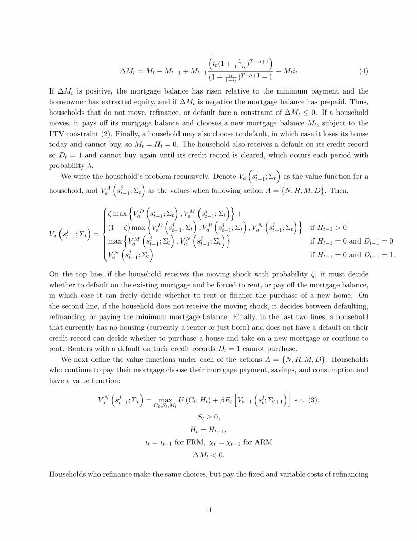
If ∆Mt is positive, the mortgage balance has risen relative to the minimum payment and the

homeowner has extracted equity, and if ∆Mt is negative the mortgage balance has prepaid. Thus,

households that do not move, refinance, or default face a constraint of ∆Mt ≤ 0. If a household

moves, it pays off its mortgage balance and chooses a new mortgage balance Mt, subject to the

LTV constraint (2). Finally, a household may also choose to default, in which case it loses its house

today and cannot buy, so Mt = Ht = 0. The household also receives a default on its credit record

so Dt = 1 and cannot buy again until its credit record is cleared, which occurs each period with

probability λ.

We write the household’s problem recursively. Denote Va

(sjt−1; Σt

)as the value function for a

household, and V Aa

(sjt−1; Σt

)as the values when following action A = N,R,M,D. Then,

Va

(sjt−1; Σt

)=

ζ maxV Da

(sjt−1; Σt

), VM

a

(sjt−1; Σt

)+

(1− ζ) maxV Da

(sjt−1; Σt

), V R

a

(sjt−1; Σt

), V N

a

(sjt−1; Σt

)if Ht−1 > 0

maxVMa

(sjt−1; Σt

), V N

a

(sjt−1; Σt

)if Ht−1 = 0 and Dt−1 = 0

V Na

(sjt−1; Σt

)if Ht−1 = 0 and Dt−1 = 1.

On the top line, if the household receives the moving shock with probability ζ, it must decide

whether to default on the existing mortgage and be forced to rent, or pay off the mortgage balance,

in which case it can freely decide whether to rent or finance the purchase of a new home. On

the second line, if the household does not receive the moving shock, it decides between defaulting,

refinancing, or paying the minimum mortgage balance. Finally, in the last two lines, a household

that currently has no housing (currently a renter or just born) and does not have a default on their

credit record can decide whether to purchase a house and take on a new mortgage or continue to

rent. Renters with a default on their credit records Dt = 1 cannot purchase.

We next define the value functions under each of the actions A = N,R,M,D. Households

who continue to pay their mortgage choose their mortgage payment, savings, and consumption and

have a value function:

V Na

(sjt−1; Σt

)= max

Ct,St,Mt

U (Ct, Ht) + βEt

[Va+1

(sjt ; Σt+1

)]s.t. (3),

St ≥ 0,

Ht = Ht−1,

it = it−1 for FRM, χt = χt−1 for ARM

∆Mt < 0.

Households who refinance make the same choices, but pay the fixed and variable costs of refinancing

11

and face the LTV constraint rather than the ∆Mt < 0 constraint. They have a value function:

V Ra

(sjt−1; Σt

)= max

Ct,St,Mt

U (Ct, Ht) + βEt

[Va+1

(sjt ; Σt+1

)]s.t. (3),

St ≥ 0,

Mt ≤ φptHt,

Ht = Ht−1,

it = iFRMt for FRM, χt = χARMt for ARM.

Households who move choose their consumption, savings, and if buying, mortgage balance, as

refinancers do, but also get to choose their housing Ht+1. They have a value function:

VMa

(sjt−1; Σt

)= max

Ct,St+1,Mt+1,Ht+1

U (Ct, Ht) + βEt

[Va+1

(sjt ; Σt+1

)]s.t. (3),

St ≥ 0,

Mt ≤ φptHt,

it = iFRMt for FRM, χt = χARMt for ARM.

Households who default lose their home but not their savings. The defaulting households choose

consumption and savings and have a value function:

V Da

(sjt−1; Σt

)= max

Ct,St

−d+ U (Ct, Ht) + βEt

[Va+1

(sjt ; Σt+1

)]s.t. (3)

St ≥ 0,

Ht = Mt = 0

Dt = 1.

In the final period, a household must liquidate its house regardless of whether it gets a moving

shock, either through moving or defaulting:

VT

(sjt ; Σt

)= max

V NT

(sTt ; Σt

), V D

T

(sTt ; Σt

).

3.3 Mortgage Spread Determination

We assume that mortgages are supplied by competitive, risk-neutral lenders.9 In the event of

default, the lender forecloses on the home, sells it in the open market, and recovers a fraction Υ of

its current value.

Define the net present value of the expected payments made by an age a household with id-

iosyncratic state sjt−1 and aggregate state Σt, which is the value of the mortgage to a lender, as

9Alternatively, it would be straightforward to allow for possible lender risk aversion by assuming a flexible, state-dependent SDF which prices the mortgages. The inclusion of such an SDF, which would be equivalent to endogenizingκ, would not change the insights of the analysis but would quantitatively affect our results.

12

Πa

(sjt−1; Σt

). This can be written recursively as:

Πa

(sjt−1; Σt

)= δ

(sjt−1; Σt

)Υpt + σ

(sjt−1; Σt

)Mt−1+ (5)(

1− δ(sjt−1; Σt

)− σ

(sjt−1; Σt

))[ Mt−1 −Mt (1− it)+ 1

1+rt+κEt

[Πa+1

(sjt ,Σt+1

)] ],where the household policy functions, σ

(sjt−1, ζ; Σt

)is an indicator for whether a household moves

or refinances, δ(sjt−1, ζ; Σt

)is an indicator for whether a household defaults, and κ > 0 is the

bank’s per-period cost of capital over the short-term interest rate. In the present period, the lender

receives the recovered value in the event of a foreclosure, the mortgage principal plus interest in the

event the loan is paid off, and the required payment on the mortgage plus any prepayments made

by the borrower if the loan continues. The lender also gets the discounted expected continuation

value of the loan at the new balance if the loan continues.

We assume that the interest rate on an FRM originated at time t, iFRMt , and the spread over

the short rate on an ARM originated at time t, χARMt , are determined competitively such that

lenders break even on average in each aggregate state given their cost of capital κ:

EΘt=Θi

[E

Ωorigt

[1

1 + rt + κΠa

(sjt ; Σt+1

)− (1− it)Mt

]]= 0 ∀ Θi ∈ Θ, (6)

where Ωorigt is the distribution of newly originated mortgages at time t. The expectation integrates

out over all periods in which Θt takes on a given value Θi and over all loans originated at time

t.10 This pools risk across borrowers but prices the mortgage to incorporate all information on the

aggregate state of the economy, Θi. By allowing the pricing to depend on the aggregate state, we

allow mortgage rates to depend on the interest rate in that state as well as the expected path of

interest rates conditional on that state, as encoded in the yield curve. We also allow pricing to

depend on the endogenous prepayment risk and default risk of mortgages as originated in a given

state. Thus, our assumptions imply that if a mortgage design shifts risks from borrowers to lenders

in a given state, the spread rises until the lenders are compensated for this risk.

Our assumption of a single spread for each aggregate state implies that there is cross-subsidization

in mortgage pricing. Because default is low in equilibrium, the amount of cross-subsidization is not

substantial.11 Moreover, in practice, there is cross-subsidization in GSE mortgage pricing: Hurst

et al. (2016) document that GSE mortgage rates for otherwise identical loans do not vary spatially.

We determine the interest rates iFRMt (Θt) and the ARM spreads χARMt (Θt) using this pricing

condition for each mortgage design. To set κ, we match data on the spread between the 10-year

Treasury bond and the average 30-year fixed rate mortgage from FRED. This spread averaged 1.65

10Mt is the end of period mortgage balance. Given the timing, the household immediately makes a mortgagepayment if itMt, and so on net the bank gives the household (1− it)Mt.

11Banks would make large losses on low-income homeowners who cannot afford their mortgage payment. However,such households cannot make a down payment and cannot afford the fixed and variable costs of home purchase andthus do not purchase in equilibrium. Those homeowners that do obtain mortgages do vary in their default risk, butit is generally low.

13

percent from 1983 to 2013. We adjust κ so that the spread between a 10-year risk-free bond with

pre-paid interest in the model with a yield determined by the expectations hypothesis and the

FRM rate in the model averages to 1.65 percent. In doing so, we convert a bond where the interest

between t and t+ 1 is paid at time t+ 1 at rate r to a bond where the interest between t and t+ 1

is paid at time t at rate i using the relationship i = r1+r .

3.4 Equilibrium

A competitive equilibrium consists of decision rules over actions A = N,R,M,D and state

variables Ct, St, Mt, Ht, a price function p(Σt), an FRM rate iFRM (Θ) and an ARM spread

χARM (Θ) for each aggregate state Θ, and a law of motion for the aggregate state variable Σt.

Decisions are optimal given the home price function and the law of motion for the state variable.

At these decisions, the housing market clears at price pt, the risk-neutral lenders break even on

average according to (6), and the law of motion for Σt is verified.

Given the fixed supply of homes, market clearing equates supply from movers, defaulters, and

investors who purchased last period with demand from renters, moving homeowners, and investors.

Let η(sjt−1, ζ; Σt

)be an indicator for whether a household moves and δ

(sjt−1, ζ; Σt

)be an indi-

cator for whether a household defaults. Movers and defaulters own Ht−1

(sjt−1; Σt

)housing, while

buyers purchase Ht

(sjt ; Σt

)housing. The housing market clearing condition satisfied by the pricing

function p (Σt) is then:∫δ(sjt−1, ζ; Σt

)Ht−1

(sjt−1; Σt

)dΩt +

∫η(sjt−1, ζ; Σ

)Ht−1

(sjt−1; Σt

)dΩt (7)

=

∫η(sjt−1, ζ; Σt

)Ht

(sjt−1; Σt

)dΩt,

where the first line side is supply which includes defaulted homes and sales and the second line is

demand.

3.5 Solution Method

Solving the model requires that households correctly forecast the law of motion for Σt which drives

the evolution of home prices. Note that Σt is an infinite-dimensional object due to the distribution

Ωt(sjt−1). To deal with this issue, we follow the implementation of the Krusell and Smith (1998)

algorithm in Kaplan, Mitman, and Violante (2017). We focus directly on the law of motion for

home prices and assume that households use a simple AR(1) forecast rule that conditions on the

state of the business cycle today Θt and the realization of the state of the business cycle tomorrow

Θt+1 for the evolution of pt:

log pt+1 = f(Θt,Θt+1) (log pt) (8)

where f(Θt,Θt+1) is a function for each realization of (Θt,Θt+1). We parameterize f (·) as a linear

spline.12 Expression (8) can be viewed either as a tool to compute equilibrium in heterogeneous-

12We have found that a linear spline performs better than a linear relationship. The relationship is approximatelylinear in periods with no default and linear in periods with some default, although the line bends when default kicks

14

agent economies, following Krusell and Smith (1998) or as an assumption that households and

investors are boundedly rational and formulate simple forecast rules for the aggregate state. To

verify that the decision rule is accurate, we both compute the R2 for each (Θt,Θt+1) realized in

simulations and follow Den Haan (2010) by comparing the realized price with the 15, 30, 45, and

100-year ahead forecasts given the realized process of aggregate shocks to verify that the forecast

rule does a good job of computing expected prices many periods into the future and that small

errors do not accumulate. The Appendix shows this is the case.

The model cannot be solved analytically, so a computational algorithm is used. First, the

household problem is solved for a given forecast rule and mortgage spreads by discretization and

backward induction. The model is simulated for 19,000 periods with the home price determined by

(7). Given the distribution of mortgages originated in each state, the break-even spread for each

aggregate state is determined according to (6), and the AR(1) forecast regression (8) is run in the

simulated data for each (Θt,Θt+1). Finally, the forecast rule is updated based on the regression

and the spread is updated based on the break-even spread, and the entire procedure is repeated

until the forecast rules and spreads converge.

4 Calibration

Our calibration proceeds in three steps. First, we select the aggregate and idiosyncratic shocks to

reflect modern business cycles in the United States. Second, we exogenously calibrate a number

of parameters to standard values in the macro and housing literature. The final parameters are

calibrated internally to match moments of the data. Our model does a good job of matching the

life cycle and population distributions of assets and mortgage debt. Furthermore, as a validation

exercise, we show that our model quantitatively matches quasi-experimental evidence on the effects

of payment reductions on default.

Throughout, we calibrate to the data using a model in which all loans are fixed rate mortgages

to reflect the predominant mortgage type in the United States. Table 1 summarizes the variables

and their calibrated values. κ, the fixed origination cost for the lender, is determined in the FRM

equilibrium under the baseline monetary policy to match the average spread between mortgage

rates and a 10-year risk-free bond and imposed in solving for the model’s equilibrium for other

mortgages and monetary policies. The calibration is annual.

4.1 Aggregate and Idiosyncratic Shocks

We consider an economy that occasionally experiences crises akin to what occurred in the Great

Recession. To trigger such a downturn, we combine a deep and persistent recession – which lowers

aggregate income and leads to more frequent negative idiosyncratic shocks – with a tightening of

credit in the form of a stricter downpayment constraints. Several papers argue that tightening

credit helped amplify the bust and model this as a tightening LTV constraint (e.g., Favilukis

et al., 2017; Justiniano et al., 2017). We consequently assume that credit always tightens in a

in. A linear spline flexibly captures this relationship. We use the discretized price grid points for our spline knotpoints.

15

Table 1: Model Parameters in Baseline Parameterization

Param Description Value Param Description Value

T Years in Life 45 cm Variable Moving Cost as % of Price 3.0%

R Retirement 35 km Fixed Moving Cost 0.1

ρ Log Income Decline in Retirement 0.35 cr Variable Refi Cost as % of Mortgage 1.0%

τ0 Constant in Tax Function 0.8 kr Fixed Refi Cost 0.04

τ1 Curvature Tax Function 0.18 da Default Cost Dist Lower Bound 53.5

γ CRRA 3.0 db Default Cost Dist Upper Bound 63.5

ξ Bequest Motive Shifter 0.5275 q Rent 0.20

ψ Bequest Motive Multiplier 250 m Maint Cost as % of Prices 2.5%

a Utility From Homeownership 6.75 ζ Prob of Moving Shock 1/9

β Discount Factor 0.95 λ Prob Default Flag Removed 1/3

Υ Foreclosure Sale Recovery % 0.654 Homeownership Rate 65.0%

φloose Max LTV, Loose Credit 95.0% φtight Max LTV, Tight Credit 80.0%

r Short Rate [0.26%, 1.32%, 3.26%] (crisis, recession, expansion)

Y agg Aggregate Income [0.0976, 0.1426, 0.1776]

See appendix for transition matrix for Θt and Y idt .

Note: This table shows parameters for the baseline calibration. Average income is normalized to one. There are fiveaggregate states, Θt ∈Crisis With Tight Credit, Recession With Tight Credit, Recession With Loose Credit,Expansion With Tight Credit, Expansion With Loose Credit, but we assume that income and monetary policy arethe same in a recession with loose or tight credit and in an expansion with loose or tight credit. The tuples ofinterest rates reflect the interest rate in a crisis, recession, and expansion, respectively.

crisis and then stochastically reverts to being loose in expansions. Since there is insufficient data

to evaluate how monetary policy differs in various credit regimes, we assume that income and

monetary policy are identical in recessions with high and low credit and expansions with high and

low credit. This implies that the transition matrix between the five aggregate states Θt ∈Crisis

With Tight Credit, Recession With Tight Credit, Recession With Loose Credit, Expansion With

Tight Credit, Expansion With Loose Credit can be represented as a transition matrix between

three states Crisis, Recession, Expansion along with a probability that credit switches form tight

to loose in the tight credit expansion state.

We calibrate the Markov transition matrix between crisis, recession, and expansion based on

the frequency and duration of NBER recessions and expansions. We use the NBER durations and

frequencies to determine the probability of a switch between an expansion and crisis or recession,

and we assume that crises happen every 75 years and that all other NBER recessions are regular

recessions. We assume that every time the economy exits a crisis or recession it switches to an

expansion and that crises affect idiosyncratic income in the same way as a regular recession but last

longer and involve a larger aggregate income drop, with a length calibrated to match the average

duration of the Great Depression and Great Recession. A regular recession reduces aggregate

income by 3.5%, while a crisis reduces it by 8.0%, consistent with Guvenen et al.’s (2014) data

on the decline in log average earnings per person in recessions since 1980. For the probability of

reverting to loose credit from tight credit in an expansion, we choose 2.0%, so that when credit

tightens it does so persistently but credit loosens quickly enough so that a large number of crises

begin in the loose credit state. Our results are not sensitive to perturbing this target. The full

16

transition matrices can be found in the appendix.

We calibrate short rates and mortgages rates during expansions and recessions to historical real

rates from 1985-2007.13 14 We find that short rates equal 1.32% on average during recessions and

3.26% during expansions. For the crisis state, we assume that the real short rate is 3.0% less than

during expansions, or 0.26%.15 As mentioned above, we set the bank cost of capital to match a

spread of 1.65% between the 30-year fixed mortgage rate and the 10-year bond rate in the data.16

We maintain these mortgage rates as we vary the mortgage contract and monetary policy to put

different contracts on the same footing. In practice, mortgage design affects monetary policy, as

we discuss in Section 7, and so with a different mortgage design the Central Bank may set different

interest rates.

For the idiosyncratic income process, we match the countercyclical left skewness in idiosyncratic

income shocks found by Guvenen et al. (2014). Left skewness is crucial to accurately capturing the

dynamics of a housing crisis because the literature on mortgage default has found that large income

shocks are crucial drivers of default. To incorporate left skewness, we calibrate log idiosyncratic

income to follow a Gaussian AR(1) with an autocorrelation of 0.91 and standard deviation of 0.21

following Floden and Linde (2001) in an expansion but to have left skewness in the shock distribution

in recessions and crises. We discretize the income process in an expansion by matching the mean

and standard deviation of shocks using the method of Farmer and Toda (2017), which discretizes

the distribution and optimally adjusts it to match the mean and variance of the distribution to

be discretized. For the bust, we add the standardized skewness of the 2008-9 income change

distribution from Guvenen et al. (2014) to moments to be matched, generating a shock distribution

with left skewness. This gives a distribution with a negative mean income change in busts and leads

to income being too volatile, so we shift the mean of the idiosyncratic shock distribution in busts

to match the standard deviation of aggregate log income in the data. In doing so, we choose

the income distribution of the newly born generations to match the lifecycle profile of income in

Guvenen et al. (2016).17 We normalize the income process so that average aggregate income is

13We use a real model to focus the model on the benefits of interest-rate indexation in a scenario like the GreatRecession. Indeed, our central points are fairly orthogonal to the literature on “mortgage tilt” and inflation, with theexception of the possibility that adjustable-rate borrowers may see their payments rise if inflation is high in a crisisand the central bank raises interest rates. We consider such a scenario in section 7.

14Our model abstracts from regional heterogeneity in the strength of housing cycles and recessions. Given suchheterogeneity, monetary policy – and mortgage design – is a somewhat blunt instrument because it does not treatdifferent regions differently. See Piskorski and Seru (2018) for a discussion of the potential gains from indexingmortgages to local economic conditions.

15In practice, interest rates adjust gradually to the aggregate state of the economy. We assume immediate ad-justment to keep the number of aggregate states tractable. With gradual adjustment, ARMs would provide lessinsurance. This is another plus for the EK convertible mortgage , as agents may want to keep their mortgage as anFRM if ARM rates are not adjusting or are adjusting the wrong way.

16In practice, the 30-year fixed rate mortgage is priced off of the 10-year Treasury bond. We use the expectationshypothesis because we need to have counterfactual predictions of how changes in short rates are passed through intolong rates and the literature on time-varying term premia remains unsettled. If term premia shocks are random, wecan ignore them. There is some evidence that term premia are higher in recessions, which would mean long ratesmove less than in our calibration. By contrast, there is some evidence that term premia overreact to monetary policyat short horizons, which would mean that long rates move more than in our calibration.

17Rather than including a deterministic income profile, we start households at lower incomes and let them stochas-tically gain income over time as the income distribution converges to its ergodic distribution. This does a good jobof matching the age-income profile in the data as shown in the Appendix.

17

equal to one.

4.2 Other Calibration Targets

We set a number of parameters to standard values in the literature or to directly match moments

in the data.

We assume households live for 45 years, roughly matching ages 25 to 70 in the data. Households

retire after 35 years, at which point idiosyncratic income is frozen at its terminal level minus a 0.35

log point retirement decrease. The tax system is calibrated as in Heathcote et al. (2017), with

τ0 = 0.80 and τ1 = 0.18. We use a discount factor of β = 0.95 and a CRRA of γ = 3.0.

Moving and refinancing involve fixed and variable costs. We set the fixed cost of moving equal

to 10% of average annual income, or roughly $5,000. The proportional costs, paid by both buyers

and sellers, equal 3% of the house value to reflect closing costs and realtor fees. Refinancing involves

a fixed cost of 4% of average annual income, or roughly $2,000, as well as variable cost equal to 1%

of the mortgage amount to roughly match average refinancing costs quoted by the Federal Reserve.

Renters pay a rent of q = 0.20 to match a rent-to-income ratio of 20%. Homeowners must pay

a maintenance cost equal to 2.5% of the house value every year. We calibrate the moving shock

ζ so that homeowners move an average of every 9 years as in the American Housing Survey. The

homeownership rate is set to match a long-run average homeownership rate of 65 percent in the

United States.

Υ, the fraction of the price recovered by the bank after foreclosure, is set to 64.5 percent. This

combines the 27 percentage point foreclosure discount in Campbell, Giglio and Pathak (2011) with

the fixed costs of foreclosing upon, maintaining, and marketing a property, estimated to be 8.5%

of the sale price according to Andersson and Mayock (2014).18

We assume that the maximum LTV at origination under loose credit is 95%, corresponding to

the highest spike in the distribution of LTV at origination in the Great Recession, and under tight

credit is 80%, which is the conforming loan limit LTV. This generates crises with a tightening of

credit that feature a price decline similar to what we observed in the Great Recession.

We finally calibrate four parameters internally. We calibrate a, the utility benefit of owning a

home, so that house prices are approximately five times the average pre-tax income in our econ-

omy.19 We choose the bequest motive parameters ψ and ξ to match the ratio of total net worth at

age 60 to age 45 in the SCF for the median and 10th percentile households. Intuitively, ψ, which

controls the overall strength of the bequest motive, is pinned down by the median growth rate,

while ξ, which controls the extent to which bequests are a luxury, is pinned down by the 10th

percentile growth rate. We finally calibrate d, the average default cost, so that in simulations of

the impulse response to a housing downturn akin to the Great Recession described below we match

that roughly 8 percent of the housing stock was foreclosed upon from 2006 to 2013 (Guren and

18Much of the literature calibrates to the “loss severity rate” defined as the fraction of the mortgage balancerecovered by the lender. We calibrate to a fraction of the price because of a recent empirical literature that finds thatin distressed markets, the loss recovery rate is much lower (e.g. Andersson and Mayock, 2014), which is consistentwith a discount relative to price rather than a constant loss severity rate.

19In the SCF, the mean price to income ratio for homeowners is 4. Because homeowners in our model are richerthan the average household, the ratio of the mean price to average income is 5.

18

Figure 1: Lifecycle Patterns: SCF vs. Model

30 40 50 60 70

Age

0

0.1

0.2

0.3

0.4

0.5

0.6

0.7

0.8

0.9

Hom

e O

wners

hip

Rate

A. Home Ownership Rate

30 40 50 60 70

Age

0

0.2

0.4

0.6

0.8

1

1.2

LT

V

B. LTV For Owners

Mean

Median

10th Pctile

90th pctile

30 40 50 60 70

Age

0

0.1

0.2

0.3

0.4

0.5

0.6

0.7

0.8

0.9

1

PT

I

C. PTI For Owners

Mean

Median

10th Pctile

90th pctile

30 40 50 60 70

Age

-1

0

1

2

3

4

5

6

7

Wealth / M

ean Incom

e

D. Liquid and Total Wealth For Full Population

Mean

Median

10th Pctile

90th pctile

Total Wealth Median

30 40 50 60 70

Age

0

0.05

0.1

0.15

0.2

0.25

0.3

0.35

Fra

ction R

efinancin

g

E. Fraction of Owners Refinancing

30 40 50 60 70

Age

0.2

0.4

0.6

0.8

1

1.2

1.4

Incom

e o

r C

onsum

ption

F. Average Income vs. Consumption

Consumption

Income

Note: This figure compares the baseline calibration of the model with all FRMs (solid lines) to SCF data from 2001 to 2007(dashed lines) in panels A-D. Panels E and F are constructed based only on the model. Panel A shows the homeownershiprate. Panel B shows the mean, median, 10th percentile, and 90th percentile of loan to value ratios for homeowners, and panelC shows the same statistics for the payment to income ratio. Panel D shows the mean, median, 10th percentile, and 90thpercentile of liquid assets along with median total wealth. Panel E shows the refinance rate, and Panel F shows consumptionand income in the model.

McQuade, 2018).20 We match these moments closely as shown in the appendix.

4.3 Lifecycle Patterns and Distributions Across the Population

The model does a good job matching the lifecycle patterns and the overall distribution of debt and

assets in the Survey of Consumer Finances for 2001, 2004, and 2007. Figure 1 shows the lifecycle

patterns, while Figure 2 shows the distributions across the population. In both figures, the pooled

SCF data for 2001 to 2007 is in dashed lines and the model analogues are in solid lines.

Panel A of Figure 1 shows the homeownership rate over the lifecycle. The model slightly

underestimates the homeownership rate of the very young and over-estimates the homeownership

rate of the middle aged.

Panels B and C of Figure 1 shows the mean, median, 10th percentile, and 90th percentile of

the loan to value ratio (LTV) and payment to income ratio (PTI) by age, and panels A and B

20We choose da and db, the bounds of the uniform distribution from which d is chosen, to add a small bit of massaround d. In the calibration, d = 58.5, da = 53.5, and db = 63.5.

19

Figure 2: Distributions Across Population: SCF vs. Model

0 0.2 0.4 0.6 0.8 1 1.2 1.4

LTV

0

0.05

0.1

0.15

0.2

0.25

0.3

0.35

Mass

A. LTV in 0.1 Bins For Homeowners

0 0.2 0.4 0.6 0.8 1

PTI

0

0.05

0.1

0.15

0.2

0.25

0.3

Mass

B. PTI in 0.025 Bins For Homeowners

-2 0 2 4 6 8 10 12

Total Wealth / Mean Income

0

0.02

0.04

0.06

0.08

0.1

0.12

0.14

0.16

0.18

Ma

ss

C. Total Wealth in 0.2 bins

-5 0 5

Liquid Wealth / Mean Income

0

0.05

0.1

0.15

0.2

0.25

0.3

0.35

0.4

Ma

ss

D. Liquid Wealth

Note: This figure compares the baseline calibration of the model with all FRMs (solid lines) to SCF data from 2001 to 2007(dashed lines). Panel A shows loan to value ratios in 10 percentage point bins for homeowners, and panel B shows the paymentto income ratio for homeowners in 0.025 bins. Panel C shows total wealth relative to mean income in bins of 0.2, while panelD shows liquid wealth relative to mean income in bins of 0.2. In all figures, the model and data are binned identically.

of Figure 2 shows the distribution of LTV and PTI across the population. The model somewhat

over-predicts the LTV ratios of the young individuals in the bottom half of the LTV distribution.

This has minimal impact on our quantitative results, however, since these homeowners are not at

risk of default when the crisis hits. The model does reasonably well in capturing the LTV and

PTI distributions across all ages, although it somewhat overstates the number of individuals with

LTVs between 80 percent and 95 percent as is the case with any model with a single hard LTV

constraint. We also find that PTIs that are too high for the old because mortgages amortize to the

end of life. Because most of the equilibrium effects in our model come from the purchase, refinance,

and default decisions of the young who have relatively high LTVs, the financial position of elderly

homeowners has little impact on our results.

Panel D of Figure 1 shows percentiles of the liquid wealth and the median of total wealth by age,

and panels C and D of Figure 2 show the distributions of total and liquid wealth in the population.

The model does a reasonably good job matching median total wealth over the lifecycle and liquid

wealth at young ages. Agents in the model accumulate more liquid assets in retirement than in

the data. Again, this is not a significant issue, as the old do not play a crucial role in the housing

market in our model. The data also has a thicker right tail of very wealthy individuals. Our

model is designed to capture the impact of credit constraints and mortgages on housing markets,

20

so capturing the extremely wealthy is not relevant for our exercise.

Finally, Panels E and F of Figure 1 show the fraction of owners refinancing and income and

consumption over the life cycle, respectively. Most refinancing is of the cash-out variety because

the FRM rate does not fluctuate dramatically due to the expectations hypothesis. Refinancing is

relatively low until retirement, at which point it jumps so that agents can smooth their consumption.

The excessive refinancing of the old is not crucial to our results because the old are not the marginal

buyer or defaulter. Income follows a standard lifecycle profile, and consumption is smoother than

income and increasing as individuals age, consistent with buffer stock models of consumption.

4.4 Calibration Evaluation Using Quasi-Experimental Evidence on Default

To evaluate the extent to which our model quantitatively captures the impact of payment reduc-

tions, we compare our model to quasi-experimental evidence from Fuster and Willen (2017). Fuster

and Willen study a sample of homeowners who purchased ALT-A hybrid adjustable-rate mortgages

during 2005-2008 period and quickly fell underwater as house prices declined. Under a hybrid ARM,

the borrower pays a fixed rate for several years (typically five to ten) and then the ARM “resets”

to a spread over the short rate once a year. These borrowers were unable to refinance because they

were almost immediately underwater, so when their rates reset to reflect the low short rates after

2008, they received a large and expected reduction in their monthly payment.

Fuster and Willen provide two key facts for our purposes. First, they show that even for ALT-A

borrowers – who have low documentation and high LTVs relative to the population – at 135 percent

LTV the average default hazard prior to reset was only about 24 percent.21 The fact that so many

households with significant negative equity do not default implies that there are high default costs.

It is also consistent with a literature that finds evidence for a “double trigger” model of default

whereby both negative equity and a shock are necessary to trigger default, as is the case for most

default in our model.

Second, Fuster and Willen use an empirical design that compares households just before and

after they get a rate reset and show that the hazard of default for a borrower receiving a 3.0 percent

rate reduction falls by about 55 percentage points.

We evaluate the extent to which our model can match Fuster and Willen’s estimates by simulat-

ing their rate reset quasi-experiment within our model. In particular, we compare the crisis default

behavior of agents in our model with a 2/1 ARM that will reset next period with the behavior

of an agent with a 1/1 ARM that has reset this period. This corresponds to the treatment and

control used by Fuster and Willen. We assume that these borrowers are an infinitesimal part of

the market, so we can consider them in partial equilibrium, and we compute their default rates at

different LTVs with the 2/1 ARM and 1/1 ARM. To deal with the fact that the ALT-A sample

used by Fuster and Willen is not representative of the population, we roughly match the assets,

age, and income of the homeowners we consider to households with hybrid ARMs that have yet

to reset in the 2007 Survey of Consumer Finances.22 Finally, we assume that homeowners have a

21This figure is based on the default hazard in months 30 to 60 in Figure 1b. Fuster and Willen measure “default”as becoming 60 days delinquent rather than an actual foreclosure, so the actual default rate might be slightly lower.

22In the SCF, we find that the ALT-A borrowers have low assets, are young, and have moderate-to-low income, asone would expect. Due to a limited number of observations, rather than using the ages and assets of households in

21

Figure 3: Fit to Fuster and Willen (2017) Natural Experiment

1 1.5 2 2.5 3

Interest Rate Decrease

0.4

0.45

0.5

0.55

0.6

0.65

0.7

0.75

0.8

% D

ecre

ase in D

efa

ult R

ate

A. Effect of Rate Reset on Default

Model

Data

0.8 0.9 1 1.1 1.2 1.3

LTV

0

0.2

0.4

0.6

0.8

1

1.2

Hazard

Rela

tive to 1

35%

LT

V

B. Effect of LTV on Default

Note: The data from Fuster and Willen (107) come from column 1 of Table A.1 in their paper, which is also used inFigure 3 of their paper. The model estimates come form comparing a 2/1 ARM to a 1/1 ARM in our model.

fixed rate corresponding to the FRM rate in the boom and reset to the ARM rate in the crisis

Figure 3 compares the calibrated model with the findings of Fuster and Willen (2015). Panel

A shows the impact of rate reductions on default in the model and Fuster and Willen’s estimates.

Overall, the fit is quite good. The model slightly over-predicts the impact of small rate reductions

on the default hazard and under-predicts the impact of large rate reductions. The right panel shows

the baseline default rate under the 2/1 ARM at various LTVs relative to the default rate at 135

percent LTV. LTV reductions have modestly larger effects than in the data until one gets below

100 percent, at which point the default hazard falls off in the model but not in Fuster and Willen’s

data.23 The model’s fit to the Fuster and Willen quasi-experimental evidence suggests that the

model will accurately capture the effect of payment and LTV changes on default.

5 ARM vs. FRM: The Economics of State Contingent Mortgages

Having created and calibrated a laboratory to study mortgage design and its interaction with

monetary policy, we now use our model to assess various mortgages. We primarily focus on a

the SCF, we assume a uniform distribution between the 25th and 75th percentiles of age and assets in the SCF dataand assume that individuals in the Fuster-Willen experiment have moderate to low income.

23Fuster and Willen find a substantial default hazard below 100 percent LTV for three likely reasons. First, thecombined LTV that Fuster and Willen use is likely measured with error both due to missing liens in the data anddue to error in the automatic valuation model. Second, Fuster and Willen measure default as 60 day delinquency andnot a final foreclosure. In areas with substantial foreclosure backlogs, borrowers who are above water can becomedelinquent before they sell. Finally, there are some frictions in terms of time to sell and the fixed costs of sale thatmay cause above-water households to default. In our model, there is minimal default for above water householdsbecause some households get a moving shock with very low equity and decide to default.

22

crisis scenario that combines a housing bust and a deep recession as in the Great Recession. This

allows us to analyze mortgage designs proposed to address the problems revealed by the Great

Recession, which is the focus of the recent literature. Additionally, the equilibrium feedbacks that

our model features are most interesting and potent in a downturn with a price-default spiral. In

this section we focus on conventional monetary policy that reduces real rates in a crisis, and we

consider alternate monetary policies, including the case in which the central bank raises real rates

in a bust, in Section 7.

To analyze a housing downturn, we simulate an impulse response where in the five years prior

to the downturn the economy is in an expansion with loose credit and when the crisis hits the

economy falls into a deep recession and the LTV constraint tightens. We assume that the crisis

lasts at least three years, after which the economy stochastically exits according to the transition

matrix so that the average crisis length is 5.66 years. We study the impulse responses of prices,

default rates, and consumption to the resulting downturn, which we compute by averaging together

100 simulations with random shocks prior to the five-year expansion and subsequent to the first

three years of the crisis. We also compare mortgage designs in stochastic simulations.

To analyze the effect of mortgage design in such a crisis, we first compare an economy with

all FRM borrowers to an economy with all ARM borrowers. This provides us with most of the

economic intuition regarding the benefits of adding state contingency to mortgages. In Section 6,

we consider more complex mortgage designs.

5.1 Economic Intuition: FRM vs. ARM

Our baseline case is an economy in which the only available mortgage to home purchasers is a

fixed-rate mortgage. The results are illustrated by the blue lines in Figure 4.

The model with all FRMs generates a housing crisis in the model of a similar magnitude to

the the one experienced in the United States between 2006 and 2012 as shown in Figure 4. Prices

fall by about a third, which closely matches the peak to trough decline in national repeat sales

house price indices.24 At the depths of the crisis, 40 percent of homeowners are underwater and

70 percent of homeowners have under 20 percent equity and cannot refinance given the tightened

LTV constraint. The combination of negative equity and recession leads 7.9 percent of the housing

stock to default (recall that matching the fraction of the housing stock that defaulted from 2006

to 2013 is a calibration target). Finally, consumption falls by 11.6 percent due to the sudden and

persistent decline in income and the large number of constrained households. The decline is slightly

higher than the decline in the data.25

We examine the differential impacts of adjustable-rate mortgages through two experiments.

In the first, we assume that home purchasers have fixed-rate mortgages pre-crisis, but that when

the crisis hits, all mortgages are unexpectedly converted to adjustable-rate mortgages with the

24Our model does not match the time series of house price indices because prices fall to their lowest level on theimpact of the shock, while in the data they decline gradually. This is the case because our Walrasian model does nothave any house price momentum. See Guren (2018) for a summary of the literature on momentum.

25With a 2.5 percent annual trend, real personal consumption expenditures fell 9.4 percent relative to trend peakto trough in the recession. Our model may have a larger decline than in the data because we do not capture theupper tail of the income distribution well and because we do not model lenders.

23

Figure 4: FRM vs. FRM→ARM: Housing Market Outcomes

-10 -5 0 5 10 15

Years

0.65

0.7

0.75

0.8

0.85

0.9

0.95

1

Price

Re

lative

to

Ye

ar

0

A. House Prices

-10 -5 0 5 10 15

Years

0

0.2

0.4

0.6

0.8

1

Price

Re

lative

to

Ye

ar

0

B. Share Negative Equity

Neg Eq, FRM

Neg Eq, FRM->ARM

<10% Eq, FRM

<10% Eq, FRM->ARM

<20% Eq, FRM

<20% Eq, FRM->ARM

-10 -5 0 5 10 15

Years

0

0.01

0.02

0.03

0.04

0.05

0.06

De

fau

lt R

ate

(F

ractio

n o

f H

ou

sin

g S

tock)

C. Default Rate

FRM

FRM->ARM

Cum Diff FRM - FRM->ARM

-10 -5 0 5 10 15

Years

0.86

0.88

0.9

0.92

0.94

0.96

0.98

1

1.02

Co

nsu

mp

tio

n/I

nco

me

Re

lative

to

Ye

ar

0

D. Consumption

Note: The figure shows the impulse response to a simulated downturn preceded by an expansion with loose credit under FRMand FRM→ARM. In the downturn, the maximum LTV falls from 95 percent to 80 percent and the economy falls into a deepdownturn for an average of 5.66 years.

spread based on the origination state of the mortgage. Because the central bank lowers the short

rate in the crisis and this is fully passed through to households under ARM, mortgage payments

fall dramatically. This experiment, which we call the FRM→ARM counterfactual, is a useful

thought experiment to understand the mechanisms at work in our model because it holds fixed

the distribution of individuals across idiosyncratic states when the crisis hits and isolates the ex-

post effect of adjustable-rate mortgages on the severity of the crisis. In the second experiment, we

consider an economy with ARMs both before and after the crisis hits, allowing for ex-ante behavior

to affect the distribution of households across idiosyncratic states at the beginning of the crisis.

5.1.1 Ex-Post Effect of Switching From FRM to ARM

The FRM→ARM counterfactual is shown in purple lines in Figure 4. Relative to the baseline case,

the housing crisis is less severe. House prices fall by 3.8 percentage points less and 33.6 percent

fewer households default.

Under FRM, the rate reduction is not passed through to households to the same extent because

24

Figure 5: FRM vs. FRM→ARM: Default and Renter Demand By Age

25 30 35 40 45 50 55 60 65 70

Age

0

2

4

6

8

Ma

ss D

efa

ultin

g

10 -4 Default by Age

FRM

FARM

Dif

25 30 35 40 45 50 55 60 65 70

Age

-1

0

1

2

3

Ma

ss B

uyin

g

10 -3 Renter Purchases by Age

FRM

FARM

Dif

Note: The figure shows the mass of households of each age defaulting and purchasing after renting last period in the firstperiod of a simulated crisis under FRM and FRM→ARM along with the difference between the two lines. To ensure thatthe differences are entirely due to the policy functions, we compare FRM to FRM→ARM and evaluate the policy functionsassuming the price is the realized FRM price.

the long end of the yield curve moves by less and because some homeowners do not have the means

to satisfy the tighter LTV constraint and cannot refinance. Because of left-skewness of the income

shock distribution in the crisis, a significant fraction of the underwater homeowners experience

a drop in their income. Those with little savings default because they would have to cut their

consumption substantially – and in many cases to zero – to make their mortgage payment, which

causes them to be willing to bear the utility cost of default. Default increases the supply of homes

on the market, further pushing down prices, which in turn leads to more default. This phenomenon

is the canonical price-default spiral.

In the ARM economy, by contrast, the mortgage payment is pegged to the prevailing short rate

in the market, so payments fall automatically. They also fall by more than under FRM because

the short end of the yield curve adjusts by more under the expectations hypothesis than the long

end. Many households that default with an FRM can avoid default, short-circuiting the default

spiral and causing a less severe housing crisis.

Additionally, because FRMs are priced off of long-term rates, which fall via the expectations

hypothesis, buying is more affordable in the ARM economy for young renters during the crisis

than in the FRM economy. This implies that the demand by renters is higher when the economy

switches to ARMs, which further ameliorates the impact of the housing crisis.

These effects are summarized in Figure 5, which plots the mass of homeowners defaulting and

renters purchasing by age in the period in which the crisis begins. The results are plotted for

both the baseline FRM economy and the FRM→ARM counterfactual, along with the difference.

Because the pre-downturn distribution is the same, this figure only reflects differences in policy

25

Figure 6: FRM vs. ARM: Housing Market Outcomes

-10 -5 0 5 10 15

Years

0.65

0.7

0.75

0.8

0.85

0.9

0.95

1

Price

Re

lative

to

Ye

ar

0

A. House Prices

-10 -5 0 5 10 15

Years

0

0.2

0.4

0.6

0.8

1

Price

Re

lative

to

Ye

ar

0

B. Share Negative Equity

Neg Eq, FRM

Neg Eq, ARM

<10% Eq, FRM

<10% Eq, ARM

<20% Eq, FRM

<20% Eq, ARM

-10 -5 0 5 10 15

Years

0

0.01

0.02

0.03

0.04

0.05

0.06

De

fau

lt R

ate

(F

ractio

n o

f H

ou

sin

g S

tock)

C. Default Rate

FRM

ARM

Cum Diff FRM-ARM

-10 -5 0 5 10 15

Years

0.86

0.88

0.9

0.92

0.94

0.96

0.98

1

1.02

Co

nsu

mp

tio

n/I

nco

me

Re

lative

to

Ye

ar

0

D. Consumption

Note: The figure shows the impulse response to a simulated downturn preceded by an expansion with loose credit under FRMand ARM both ex ante and ex post . In the downturn, the maximum LTV falls from 95 percent to 80 percent and the economyfalls into a deep downturn for an average of 5.66 years.

functions between the FRM and FRM→ARM economies. The gap in default is dominated by

young and middle-aged households, and the gap in renter purchases is dominated by homebuyers

around the age of first purchase. Similar comparisons by savings, income, and LTV reveal that

the additional default under FRM comes from low income, low savings, and high LTV borrowers,

while the additional demand comes from renters with the moderate savings and income reflective

of first-time homebuyers.

5.1.2 Ex-Ante Effect of Switching From FRM to ARM

Of course, while useful for expositional purposes, the economy in which all mortgages suddenly

switch to ARMs is unrealistic. We therefore now instead consider an economy in which all mortgages

are adjustable-rate, both pre- and post-crisis. The results are presented in Figures 6, with the FRM

economy shown in blue and the ARM economy shown in orange.

The benefits of adjustable-rate mortgages are reduced relative to the FRM→ARM counterfac-

tual, with prices falling by 2.7 percentage points and 26.1 percent fewer households defaulting than

26

Table 2: FRM vs. ARM: Pre-Crisis LTV and Savings Distribution Differences

Ages 26-45 36-45

Owners With Savings Under .5, ARM - FRM 2.38% 2.27%Renters With Savings Above 1, ARM - FRM -0.23% -0.76%

Owners With LTV > 0.9, ARM - FRM 0.20% 0.30%

Note: Each panel shows the difference in the percentage of owners or renters satisfying each criteria based on the averagedistribution in the pre-dowtnurn period from 100 impulse response simulations. Each row shows the difference between theARM and FRM economies.

under FRM rather than 3.8 percentage points and 33.5 percent under FRM→ARM. These figures

are summarized for ARM and the mortgage designs we consider subsequently in Table 3.

The crisis is worse in the ARM economy relative to the FRM→ARM economy for two reasons.

First, young homeowners understand the hedging properties of the ARM mortgage and take on more

risk by both increasing their LTV and holding less savings in order to increase their consumption

in constrained states. This creates macro fragility, which households do not internalize. Second,

young renters hold less savings, and so fewer are able to meet the down payment in the bust, which

increases despite the lower price due to the tightened LTV constraint. The effect of switching to

ARM ex ante on the LTV and savings distributions of young agents is shown in Table 2. Under

ARM there are more young owners with low savings and high LTV and fewer young renters with

high savings. The degree to which the ex-post benefits of ARMs are undone by the ex-ante buildup

of fragility – at least for house prices and default – is a numerical result. This highlights the need

for realistic quantitative models of the type we analyze.

5.1.3 Welfare Benefits of Switching From FRM to ARM

To further evaluate the benefits of switching from FRM to ARM, we calculate the consumption-

equivalent welfare cost of the crisis under each mortgage for generations that are alive when the

crisis hits. To do so, we calculate how much each agent would be willing to reduce their consumption

per year of their remaining life to avoid a crisis. This is calculated as equivalent variation and is

aggregated by the pre-crisis distribution of individuals across states for agents living when the crisis

hits, as detailed in the Appendix. Welfare relative to the FRM economy is shown for ARM and

the mortgage designs we consider subsequently in Table 3.

Households alive when the crisis hits would be willing to give up 0.83 percent more of their

annual consumption for their remaining life to avoid the crisis in the FRM economy than the ARM

economy. However, this aggregate calculation masks substantial heterogeneity across groups, as

shown in Figure 7, which reports the welfare difference separately by age, LTV in the first period of

the crisis, savings, and idiosyncratic income for both renters and owners. A negative value indicates

a larger welfare loss under FRMs than in the ARM counterfactual, and all figures are in percentage

points of consumption.

Figure 7 reveals that the welfare benefits of ARMs are concentrated on two groups. The first

group is young, low savings, low income, and high LTV homeowners, who would be willing to

give up as much as four percent more of their annual consumption to avoid the crisis in the FRM

27

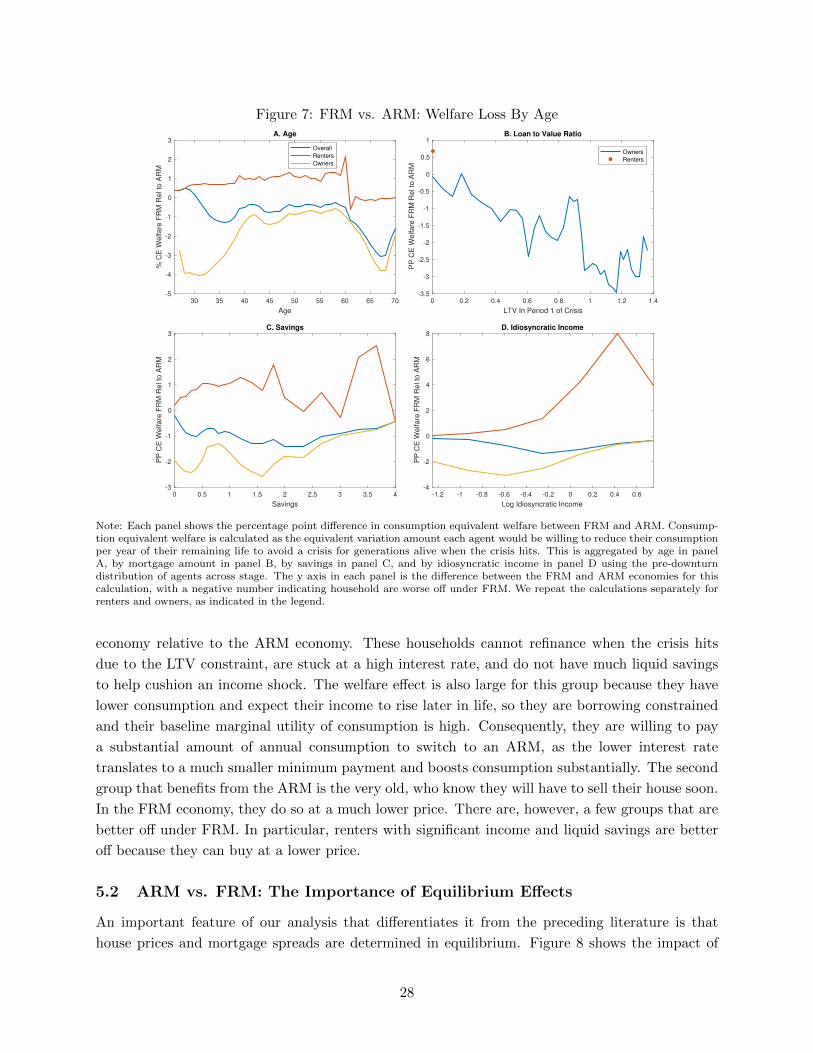
Figure 7: FRM vs. ARM: Welfare Loss By Age

30 35 40 45 50 55 60 65 70

Age

-5

-4

-3

-2

-1

0

1

2

3

% C

E W

elfa

re F

RM

Rel to

AR

M

A. Age

Overall

Renters

Owners

0 0.2 0.4 0.6 0.8 1 1.2 1.4

LTV In Period 1 of Crisis

-3.5

-3

-2.5

-2

-1.5

-1

-0.5

0

0.5

1

PP

CE

Welfa

re F

RM

Rel to

AR

M

B. Loan to Value Ratio

Owners

Renters

0 0.5 1 1.5 2 2.5 3 3.5 4

Savings

-3

-2

-1

0

1

2

3

PP

CE

Welfa

re F

RM

Re

l to

AR

M

C. Savings

-1.2 -1 -0.8 -0.6 -0.4 -0.2 0 0.2 0.4 0.6

Log Idiosyncratic Income

-4

-2

0

2

4

6

8

PP

CE

Welfa

re F

RM

Re

l to

AR

M

D. Idiosyncratic Income

Note: Each panel shows the percentage point difference in consumption equivalent welfare between FRM and ARM. Consump-tion equivalent welfare is calculated as the equivalent variation amount each agent would be willing to reduce their consumptionper year of their remaining life to avoid a crisis for generations alive when the crisis hits. This is aggregated by age in panelA, by mortgage amount in panel B, by savings in panel C, and by idiosyncratic income in panel D using the pre-downturndistribution of agents across stage. The y axis in each panel is the difference between the FRM and ARM economies for thiscalculation, with a negative number indicating household are worse off under FRM. We repeat the calculations separately forrenters and owners, as indicated in the legend.

economy relative to the ARM economy. These households cannot refinance when the crisis hits

due to the LTV constraint, are stuck at a high interest rate, and do not have much liquid savings

to help cushion an income shock. The welfare effect is also large for this group because they have

lower consumption and expect their income to rise later in life, so they are borrowing constrained

and their baseline marginal utility of consumption is high. Consequently, they are willing to pay

a substantial amount of annual consumption to switch to an ARM, as the lower interest rate

translates to a much smaller minimum payment and boosts consumption substantially. The second

group that benefits from the ARM is the very old, who know they will have to sell their house soon.

In the FRM economy, they do so at a much lower price. There are, however, a few groups that are

better off under FRM. In particular, renters with significant income and liquid savings are better

off because they can buy at a lower price.

5.2 ARM vs. FRM: The Importance of Equilibrium Effects

An important feature of our analysis that differentiates it from the preceding literature is that

house prices and mortgage spreads are determined in equilibrium. Figure 8 shows the impact of

28

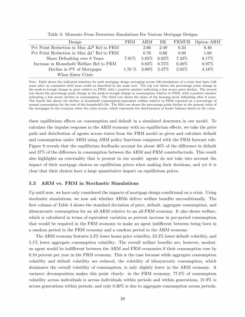
Table 3: Moments From Downturn Simulations For Various Mortgage Designs

Design FRM ARM EK FRMUR Option ARM

Pct Point Reduction in Max ∆P Rel to FRM 2.66 2.49 0.34 6.46Pct Point Reduction in Max ∆C Rel to FRM 0.76 0.66 0.08 1.60

Share Defaulting over 8 Years 7.91% 5.85% 6.02% 7.32% 6.17%Increase in Household Welfare Rel to FRM 0.83% 0.75% 0.20% 0.97%

Decline in PV of Mortgages 1.70 % 2.89% 2.47% 2.05% 3.18%When Enter Crisis

Note: Table shows the indicated statistics for each mortgage design averaging across 100 simulations of a crisis that lasts 5.66years after an expansion with loose credit as described in the main text. The top row shows the percentage point change inthe peak-to-trough change in price relative to FRM, with a positive number indicating a less severe price decline. The secondrow shows the percentage point change in the peak-to-trough change in consumption relative to FRM, with a positive numberindicating a less severe decline in consumption. The third row shows the share of the housing stock defaulting after 8 years.The fourth line shows the decline in household consumption-equivalent welfare relative to FRM reported as a percentage ofannual consumption for the rest of the household’s life. The fifth row shows the percentage point decline in the present value ofthe mortgages in the economy when the crisis occurs, which represents the deterioration of lender balance sheets in the crisis.

these equilibrium effects on consumption and default in a simulated downturn in our model. To

calculate the impulse response in the ARM economy with no equilibrium effects, we take the price

path and distribution of agents across states from the FRM model as given and calculate default

and consumption under ARM using ARM policy functions computed with the FRM forecast rule.

Figure 8 reveals that the equilibrium feedbacks account for about 46% of the difference in default

and 37% of the difference in consumption between the ARM and FRM counterfactuals. This result

also highlights an externality that is present in our model: agents do not take into account the

impact of their mortgage choices on equilibrium prices when making their decisions, and yet it is

clear that their choices have a large quantitative impact on equilibrium prices.

5.3 ARM vs. FRM in Stochastic Simulations

Up until now, we have only considered the impacts of mortgage design conditional on a crisis. Using

stochastic simulations, we now ask whether ARMs deliver welfare benefits unconditionally. The

first column of Table 4 shows the standard deviation of price, default, aggregate consumption, and

idiosyncratic consumption for an all-ARM relative to an all-FRM economy. It also shows welfare,

which is calculated in terms of equivalent variation as percent increase in per-period consumption

that would be required in the FRM economy to make an agent indifferent between being born in

a random period in the FRM economy and a random period in the ARM economy.

The ARM economy features 3.3% lower house price volatility, 23.3% lower default volatility, and

5.1% lower aggregate consumption volatility. The overall welfare benefits are, however, modest:

an agent would be indifferent between the ARM and FRM economies if their consumption rose by

0.10 percent per year in the FRM economy. This is the case because while aggregate consumption

volatility and default volatility are reduced, the volatility of idiosyncratic consumption, which

dominates the overall volatility of consumption, is only slightly lower in the ARM economy. A

variance decomposition makes this point clearly: in the FRM economy, 77.8% of consumption

volatility across individuals is across individuals within periods and within generations, 21.9% is

across generations within periods, and only 0.30% is due to aggregate consumption across periods.

29

Figure 8: FRM vs. ARM: The Role of Equilibrium Effects

-10 -5 0 5 10 15

Years

0

0.005

0.01

0.015

0.02

0.025

0.03

0.035

0.04

Defa

ult R

ate

(F

raction o

f H

ousin

g S

tock)

A. Default Rate

FRM

ARM

ARM No Equilibrium Effects

Cum Diff

Cum DiffNo Equilibrium Effects

-10 -5 0 5 10 15

Years

0.86

0.88

0.9

0.92

0.94

0.96

0.98

1

1.02

Con

sum

ption/Incom

e R

ela

tive t

o Y

ear

0

B. Consumption

Note: The figure shows the impulse response to a simulated downturn preceded by an expansion with loose credit under FRMand ARM both ex ante and ex post . In the downturn, the maximum LTV falls from 95 percent to 80 percent and the economyfalls into a deep downturn for an average of 5.66 years. For the “no equilibrium effects” counterfactual, we take the pricepath and distribution of agents across states from the FRM model as given and report default and consumption using policyfunctions computed with ARMs with the FRM forecast rule.

Since ARMs only provide insurance against aggregate shocks, the consumption insurance benefits

in normal times are modest. This does, however, open the door for mortgage designs that provide

insurance against idiosyncratic risk, a point we return to in the next section.

As we have seen, for particularly severe crises, ARMs can dramatically reduce housing market

volatility. Together with the reduced volatility of aggregate variables under ARMs, our results sug-

gest that indexing mortgages to aggregate conditions through ARMs provides important insurance

to the macroeconomy.

6 Evaluating New Mortgage Designs

We have so far focused on comparing ARMs and FRMs to clearly elucidate the insurance benefits

of indexation. However, ARMs have some drawbacks. In particular, if the central bank raises

interest rates to fight an inflationary recession, our assumption that in recessions short rates fall

may be violated. In these cases, ARMs are worse from an insurance perspective, the reverse of our

main results because the covariance of interest rates and income shocks switches sign. We show

this quantitatively in Section 7. Furthermore, by revealed preference, most Americans prefer fixed

rate mortgages, which on average account for roughly 80 percent of mortgage originations.26

Given these downsides, in this section we evaluate several mortgage designs that allow for state

contingency in a crisis while preserving the benefits of FRMs in normal times. We also evaluate

a contract that provides more idiosyncratic insurance than a standard ARM. Our main finding is

that mortgage designs that front-load payment relief in the crisis outperform mortgages that spread

26If we allow for both FRMs and ARMs in our model about half of mortgage holders choose an ARM. However,with a small subsidy on the order of 20 basis points for the FRM we obtain a realistic ARM share. Such a subsidyis reasonable given that the FRM is institutionalized by Fannie Mae and Freddie Mac, which provide an effectivesubsidy for conforming (predominantly FRM) loans.

30

Table 4: Moments From Stochastic Simulations For Various Mortgage Designs Relative to FRM

Design ARM EK FRMUR Option ARM

Std Dev of Price Rel to FRM 96.7% 97.3% 101.4% 91.1%St Dev of Default Rate Rel to FRM 76.7% 79.9% 81.0% 71.5%

St Dev of Agg Consumption Rel to FRM 94.9% 95.6% 101.0% 89.5%St Dev of Consumption Within Periods 99.4% 99.2% 99.7% 97.8%

Across Generations Rel to FRMSt Dev of Consumption Within Periods 99.8% 99.7% 99.9% 99.1%

Within Generations Rel to FRMIncrease in Welfare Rel to FRM 0.10% 0.09% 0.03% 0.44%

Notes: All series are percentages relative to the same statistic for the indicated FRM model. Price, default, andaggregate consumption are calculated from aggregate 6,400 year simulations. Idiosyncratic consumption is calculatedby simulating 25,000 individuals each periods for 6,300 years. Welfare is calculated as the equivalent variation interms of the percent increase in annual consumption an agent would require in the FRM economy to be indifferentbetween being born in a random period in the indicated economy instead of the FRM economy.

payment relief over the life of the mortgage, even though the impact on lender balance sheets during

the crisis is similar.

6.1 Eberly-Krishnamurthy Convertible Mortgage

Eberly and Krishnamurthy (2014) propose a fixed-rate mortgage that can at any time be costlessly

converted to an adjustable-rate mortgage, but not back. This is similar to an economy in which

one can choose between ARM and FRM with two important distinctions. First, homeowners who

do not satisfy the LTV constraint can still switch to an ARM. Since in our simulated crisis 70

percent of homeowners have under 20 percent equity at the beginning of the crisis, this is likely to

be significant. Second, homeowners who are so highly constrained that they cannot afford to pay

the fixed costs of refinancing can convert to an ARM costlessly. We introduce an EK mortgage

into our model by adding an additional agent-specific state that indicates whether an agent has a

mortgage functioning as an ARM or as an FRM and allowing agents to choose to convert their loan

from an FRM to an ARM but not back without refinancing.27 Otherwise, the model is unchanged.

This mortgage has two added benefits. First, introducing it in practice is likely to be less

disruptive, as it can act exactly like a FRM and does not take away the FRM option. Second, in

the event that the covariance of interest rates and monetary policy changes, it performs more like

an FRM, as we show in Section 7.

The convertible mortgage does, however, come at a cost, as borrowers will convert to an ARM

when it is beneficial for them to do so and then refinance into a new loan that starts as an FRM

when this is no longer the case. Because ARM rates are lower than FRM rates when rates fall,

this behavior reduces the NPV of a new mortgage to the lender through standard prepayment

27There are five equations to price the EK mortgage but ten rates: an FRM rate and an ARM spread for eachstate. One must thus make a further assumption about the relationship between the FRM rate and ARM spread.We assume that when converted to ARM, the EK mortgage has the same spread over the short rate as the EKmortgage acting as an FRM has over the model-generated 10-year risk-free bond rate. The EK looks more appealingfor households if lenders make losses under ARM and profits under FRM because the decline in the rate when themortgage is converted is larger.

31

Figure 9: Eberly-Krishnamurthy Convertible Mortgage: Housing Market Outcomes

-10 -5 0 5 10 15

Years

0.65

0.7

0.75

0.8

0.85

0.9

0.95

1

Price

Re

lative

to

Ye

ar

0

A. House Prices

-10 -5 0 5 10 15

Years

-0.01

0

0.01

0.02

0.03

0.04

0.05

De

fau

lt R

ate

(F

ractio

n o

f H

ou

sin

g S

tock)

B. Default Rate

FRM

EK

Cum Diff FRM-EK

-10 -5 0 5 10 15

Years

0.86

0.88

0.9

0.92

0.94

0.96

0.98

1

1.02

Co

nsu

mp

tio

n/I

nco

me

Re

lative

to

Ye

ar

0

C. Consumption

The figure shows the impulse response to a simulated downturn preceded by an expansion with loose credit under FRM andthe Eberly-Krishnamurthy convertible mortgage both ex ante and ex post . In the downturn, the maximum LTV falls from 95percent to 80 percent and the economy falls into a deep downturn for an average of 5.66 years.

risk and results in a higher spread. The negative effect of prepayment risk on the NPV of a new

loan is partially offset by the reduced losses due to default under the EK mortgage. On net, the

prepayment risk dominates and the EK convertible mortgage on average has a 17 basis point higher

spread over the riskless 10-year bond rate than an FRM.28

Figure 9 shows a simulated downturn under the convertible mortgage. The crisis is roughly 90

percent of the way to the all-ARM economy and realizes many of the consumption-smoothing and

macroprudential benefits of ARMs. This is the case because on average the share of mortgages that

are functioning as ARMs rises from 12.7 percent pre crisis to near 100 percent during the crisis as

households who need the payments relief the most convert. The convertible mortgage does not look

fully like an ARM because of the higher spread. On net, the consumption equivalent welfare gain

relative to the FRM is 0.75 percent of consumption, compared to 0.83 percent for the ARM. Table

4 compares the Eberly-Krishnamurthy mortgage with an FRM in stochastic simulations and also

finds it is most of the way to the ARM economy. Once again, however, the unconditional welfare

effects are modest at 0.06% of annual consumption because the EK mortgage does not help insure

households against idiosyncratic risk.

6.2 Fixed Rate Mortgage With an Underwater Refinancing Option

The second mortgage that we consider is a fixed-rate mortgage that has a built-in refinance option,

which can be exercised even if the origination LTV constraint is no longer satisfied.29 We introduce

28The average spread is are calculated as an average of the spread for originating in each state weighted by theshare of loans originating in each state.

29We model this mortgage as an FRM with a built-in option to convert to a new FRM. Upon exercise of the option,the homeowner continues to pay the same spread over the 10-year bond rate as at origination but instead over thecurrent 10-year risk-free bond rate, which the household locks in for the remainder of the mortgage. Since the 10-year

32

Figure 10: FRM With an Underwater Refinancing Option: Housing Market Outcomes

-10 -5 0 5 10 15

Years

0.65

0.7

0.75

0.8

0.85

0.9

0.95

1

Price

Re

lative

to

Ye

ar

0

A. House Prices

-10 -5 0 5 10 15

Years

-0.01

0

0.01

0.02

0.03

0.04

0.05

De

fau

lt R

ate

(F

ractio

n o

f H

ou

sin

g S

tock)

B. Default Rate

FRM

FRMUR

Cum Diff FRM-FRMUR

-10 -5 0 5 10 15

Years

0.86

0.88

0.9

0.92

0.94

0.96

0.98

1

1.02

Co

nsu

mp

tio

n/I

nco

me

Re

lative

to

Ye

ar

0

C. Consumption

The figure shows the impulse response to a simulated downturn preceded by an expansion with loose credit under FRM andthe FRM with underwater refinancing both ex ante and ex post . In the downturn, the maximum LTV falls from 95 percent to80 percent and the economy falls into a deep downturn for an average of 5.66 years.

this our model by adding an additional agent-specific state that indicates whether an agent has

exercised the built-in refinance option. We assume the structure is such that the option can only

be exercised in the crisis state.

FRM with an underwater refinancing option (FRMUR) acts like an FRM except it directly

addresses the issue of not being able to refinance when one is underwater. Because payments fall

in bad states, it helps smooth consumption and reduce default losses for lenders. Of course, the

option itself is costly for lenders. On net, in our model, the FRM with an underwater refinancing

option has a 0.7 basis point higher spread than an FRM.

Figure 10 shows the crisis under FRMs with an underwater refinancing option. The FRMUR

is priced off the long end of the yield curve, which falls less than the short end in a crisis. Because

the insurance it provides is minimal, consumption is roughly the same as FRMs in the crisis. The

initial decline in prices is similar, only 7.5% fewer households default, and welfare rises by 0.20

percent of annual consumption, one quarter the gain under EK. In stochastic simulations, the

FRMUR option behaves much like an FRM with slightly lower default volatility and has essentially

no welfare gain relative to FRM, as shown in Table 4. Overall, allowing for underwater refinancing

provides some limited macroprudential benefits in a crisis but only limited consumption-smoothing

benefits because the FRM is priced off the long end of the yield curve.

The comparison of the Eberly-Krishnamurthy convertible mortgage and the FRM with an

bond rate falls during the crisis, the borrower faces a lower payment. These choices put the FRMUR mortgage on anequal footing with the EK mortgage in the sense that the original lender prices the built-in option to refinance intothe pre-crisis mortgage rate. If we were to require that a new lender take on the additional risk through refinancing,the FRMUR would look worse because rates would rise in the crisis as borrowers with a high risk of default wouldrefinance. With higher rates in the crisis, the payment relief from being able to refinance would be reduced. See theAppendix for a quantitative comparison.

33

underwater refinancing option provides the clearest contrast for our central finding: it is best to

“front load” payment relief so that it is concentrated in a crisis. Both the EK and FRMUR provide

insurance to underwater borrowers, however the EK front loads the relief by delivering maximal

relief in a recession while the FRMUR gives households a new lower fixed rate that they keep for

longer, thereby spreading the payment relief over the length of the mortgage. From the perspective

of a lender entering the crisis state, these two mortgages are quite similar. Indeed, the present

value of outstanding mortgages falls by 2.05 percent upon entering the crisis under FRMUR and

by 2.47 percent under EK, which is not a substantial difference. These figures are similar because

lenders who are not liquidity constrained are indifferent as to the timing of payments. However, the

convertible mortgage helps liquidity constrained households in the crisis by four times as much and

stems the tide of default and the price-default spiral. It also makes buying much more affordable

for new homeowners, helping put a floor under house prices. The convertible mortgage does hit

household balance sheets more when rates rise, but by then the macroeconomy and housing market

have stabilized, and house prices have recovered so that most households can refinance back into

a new mortgage that initially functions as an FRM if they so choose. Consequently, designs that

front-load the benefits of rate reductions so that they are concentrated in recessions do best in our

quantitative analysis.

One aspect of refinancing that this analysis misses is the ability of underwater homeowners

to extend their mortgage, as all mortgages amortize over the remaining lifetime of the borrower.

For, example, refinancing a loan that amortizes over 10 remaining years into a 30 year loan would

substantially lower monthly payments, even if the loans are at the same interest rate and have the

same principal (Lucas et al., 2011). Since the key issue during the crisis is liquidity, our analysis

shows that such a reduction in payments could deliver benefits. However, there are a few important

caveats. First, we have shown that the benefits are largest when payment reductions are front-

loaded, and extending an FRM’s term reduces payments over the remaining life of the mortgage

rather than front-loading them. Moreover, the benefits of obtaining a new 30-year mortgage depend

on how many years the borrower has left on her current mortgage. The households most at risk

of default and in need of liquidity in the model are largely young households who have recently

purchased a home and for whom the term extension would have a small impact, as their existing

mortgage is already a relatively long-term mortgage. Indeed, in Agarwal et al.’s (2017) analysis of

the HARP program, the average refinanced loan under HARP received a term extension of only

4.7 years. Since little principal is paid down in the first several years of the loan, this implies that

over three quarters of the payment relief from HARP came from rate reductions and less than one

quarter from principal reductions.

Finally, the FRMUR is similar to ex post policies that refinance borrowers who are underwater,

such as the Home Affordable Refinance Program pursued in the Great Recession. However, the

HARP program occurred at least in part while the Federal Reserve pursued quantitative easing, and

Agarwal et al. (2017) report that the average HARP borrower experienced a 1.4 percent reduction

in their mortgage rate, while in our baseline calibration the reduction is 0.61 percent. We show

how FRMUR interacts with quantitative easing in Section 7.2.

34

6.3 Option ARM

We now consider a mortgage design that takes maximal advantage of front-loading benefits, an

option ARM. This is an ARM mortgage that became popular in the early 2000s boom allowing the

borrower to make one of three payments: a fully amortizing payment, an interest only payment,

and a potentially negatively amortizing payment equal to the minimum payment based on the

interest rate at origination. The negative amortization is allowed up to a ceiling, and after several

years, the option ARM converts to a fully amortizing ARM. The key feature of the option ARM is

the ability to delay payments, which is potentially extremely beneficial to a homeowner in a crisis.

Piskorski and Tchistyi’s (2010) theoretical analysis of mortgage contracts with exogenous house

prices highlights the benefits of an option ARM.

Note that relative to the contracts we have considered thus far, the option ARM allows the

payment reduction to be a function of the borrower’s idiosyncratic state and not just the aggregate

state. In other words, a borrower who receives a negative income shock income in an expansion

state can choose to defer payments. The ARM or the EK contract only allow for reduced payments

in the recession or crisis state when interest rates are low. Thus our analysis of the option ARM

also captures the benefits of mortgage contracts whose payments can be indexed to idiosyncratic

states.

To introduce the option ARM in our model, we assume that the mortgage behaves like a normal

ARM for households in the last 25 years of their life. However, households in the first 20 years

of life are able to choose a mortgage balance next period equal to the maximum of their current

balance and the maximum balance allowed under the LTV constraint φ in the period in which they

took out their mortgage given today’s price. This allows for some negative amortization up to a

ceiling defined by φ, and makes it so that households are not forced to pay down principal when

the LTV constraint tightens at the beginning of the crisis.

Figure 11 compares the crisis under FRM and the option ARM. The option ARM delivers

substantially smaller price declines than the ARM in Figure 6, as prices fall by 6.46 percentage

points rather than 2.66 percentage points under ARM. The decline in aggregate consumption is

also 1.60 percentage points smaller than FRM rather than 0.76 percentage points under ARM.

However, there is more default than under ARM.

The option ARM is successful because in addition to indexing payments to the short rate as with

a standard ARM, it delivers additional front-loaded relief by allowing homeowners to negatively

amortize up to a cap during the crisis and defer mortgage payments until after the crisis. There is an

offsetting effect because homeowners understand the additional insurance benefits the option ARM

design provides and they take on more leverage when purchasing a home. Some also take advantage

of the negative amortization option before the crisis to deal with an idiosyncratic shock. This

implies that households hold fewer liquid assets and have higher LTV ratios in non-crisis periods

relative to an economy with a standard ARM, which creates macro fragility that undoes some of

the benefits of the option ARM when the crisis hits. To illustrate this, Figure 11 shows in dashed

lines an FRM→OARM counterfactual that preserves the pre-crisis distribution of individuals across

states from the FRM model by switching the economy from FRM to OARM by surprise when the

crisis hits, as with the FRM→ARM counterfactual in Section 5.1. One can see that absent the

35

Figure 11: Option ARM: Housing Market Outcomes

-10 -5 0 5 10 15

Years

0.65

0.7

0.75

0.8

0.85

0.9

0.95

1

Price

Re

lative

to

Ye

ar

0

A. House Prices

-10 -5 0 5 10 15

Years

0

0.01

0.02

0.03

0.04

0.05

0.06

De

fau

lt R

ate

(F

ractio

n o

f H

ou

sin

g S

tock)

B. Default Rate

FRM

OARM

Cum Diff FRM - OARM

FRM->OARM

Cum Diff FRM - FRM->OARM

-10 -5 0 5 10 15

Years

0.86

0.88

0.9

0.92

0.94

0.96

0.98

1

1.02

Co

nsu

mp

tio

n/I

nco

me

Re

lative

to

Ye

ar

0

C. Consumption

The figure shows the impulse response to a simulated downturn preceded by an expansion with loose credit under FRM, theoption ARM mortgage, and an FRM→OARM counterfactual. In the downturn, the maximum LTV falls from 95 percent to 80percent and the economy falls into a deep downturn for an average of 5.66 years.

endogenous increase in leverage and decrease in liquid asset holdings at the beginning of the crisis

under OARM, the price and consumption declines would have been ameliorated even more, and the

default rate would have been much lower under the option ARM. Indeed, the fact that the option

ARM preforms worse than the ARM for default is due entirely to the rightward shift in the LTV

distribution and reduction in liquid asset holdings.

It is also worthwhile to note that the option ARM provides higher welfare benefits uncondition-

ally than the other mortgage designs, as reported in Table 4. This once again is intuitive. The other

mortgage designs only provide state-contingent insurance against aggregate shocks, since changes

in interest rates are tied to aggregate movements in the economy. However, households are exposed

to substantial idiosyncratic risks. Unlike the other mortgage designs, the option ARM provides

for insurance against such shocks because young households can negatively amortize in response to

a purely idiosyncratic income shock. As a result, consumption equivalent welfare is 0.44% higher

under option ARM than FRM.

These latter observations also hint at the Achilles’ heel of the option ARM (or any similar

contract with insurance against idiosyncratic income shocks). In a model with heterogeneity in

types in which some households have low default utility costs and others have high default costs,

the option ARM will attract types with low default costs who will take the mortgage, continually

delay payments, and eventually default. Such behavior will raise the cost of the option ARM and

even unravel the market so that there is little insurance benefit from the contract. On the other

hand, with the EK mortgage or a regular ARM, the ability to delay payments is contingent on the

aggregate state, which is less subject to gaming. Our purpose in studying the option-ARM is not to

identify it as the optimal design but simply to quantify the benefit of the additional front-loading

it provides absent adverse selection concerns.

36

7 The Interaction of Mortgage Design and Monetary Policy

We now turn to examining how monetary policy interacts with mortgage design in a crisis. We begin

by comparing the polar opposite case from our main analysis in which the real interest rate rises in a

recession. We then turn to more aggressive monetary policy in a crisis both through more aggressive

short rate reductions and quantitative easing. Our model allows us to quantitatively compare how

different combinations of monetary policy and mortgage designs affect the economy. A principal

conclusion is that the FRMUR design together with quantitative easing policy commensurate to

2008-2009 does not outperform an ARM or EK along with conventional monetary policy. This

analysis highlights the value of studying mortgage design and monetary policy jointly.

7.1 Fighting Inflation: Rising Real Rates in a Crisis

In this subsection we consider a housing-led recession with substantial inflation that causes the

central bank to raise the real interest rate to contain inflationary pressures. One can think of this

as a combination of the housing bust in the Great Recession and the inflation experienced in the

1981-2 recession. To consider this case, we keep the same calibration but increase the real short

rate in a crisis to 5.6 percent, which is the average real rate in the 1981-2 recession instead of 0.26

percent.30 31 We call this the “Volcker monetary policy.”

Figure 12 shows ARM, FRM, and EK, in a simulated crisis under this alternate monetary policy.

FRMUR is not shown because it is indistinguishable from FRM when rates rise in a crisis. Because

the covariance of the short rate and income has the opposite sign from under the baseline monetary

policy, an ARM makes the household’s income stream net of mortgage payments more volatile and

leads to higher price volatility and default and lower consumption. Quantitatively, prices fall by

1.8 percentage points more under ARM, and 13.5 percent of the housing stock defaults over eight

years under ARM relative to 10.3 percent under FRM. On net, under ARM, welfare is lower by an

equivalent of 0.72 percent of annual consumption.

The EK convertible mortgage performs closer to an FRM under the Volcker monetary policy.

Prices fall by roughly the same amount peak to trough as FRM although they fall slightly more in

the first period, and the cumulative default rate over eight years is 10.9 percent. Most households

that take out a new mortgage or refinance do not convert their EK mortgage from fixed-rate to

adjustable-rate, and the ARM share at the beginning of the crisis is 12.9 percent. However, a

few households convert their EK mortgage to adjustable-rate and do not refinance into a new EK

mortgage that begins as a fixed-rate prior to the crisis. Some of these households experience an

adverse income shock in the crisis, are underwater, and end up defaulting, which is why default

is slightly higher under EK. That being said, the crisis is nowhere near as severe as under ARM

because the vast majority of households have an EK mortgage that is functioning as a FRM, which

is why EK provides a nice balance of insuring against catastrophe in an inflationary environment

30Combining the 2006-8 credit crunch with the 1981-2 recession results in rather extreme event, especially giventhat the Federal Reserve may not have raised rates as much in the 1981-2 recession in an all-ARM economy. Wenonetheless evaluate this extreme event in order to stress-test our mortgage designs.

31Many ARMs have a ceiling on the amount that the interest rate can rise over the course of the loan. In thiscounterfactual, we assume that there are no such ceilings. If there were, the increase in the ARM interest rate wouldbe smaller, but knowing this banks would increase the ex ante mortgage spread.

37

Figure 12: Short Rate Rises in Crisis as in 1981-2 Recession

-10 -5 0 5 10 15

Years

0.65

0.7

0.75

0.8

0.85

0.9

0.95

1

Price

Re

lative

to

Ye

ar

0

A. House Prices

-10 -5 0 5 10 15

Years

0

0.01

0.02

0.03

0.04

0.05

0.06

0.07

De

fau

lt R

ate

(F

ractio

n o

f H

ou

sin

g S

tock)

B. Default Rate

FRM

ARM

EK

-10 -5 0 5 10 15

Years

0.88

0.9

0.92

0.94

0.96

0.98

1

1.02

Co

nsu

mp

tio

n/I

nco

me

Re

lative

to

Ye

ar

0

C. Consumption

Note: The figure shows the outcomes in a simulated downturn in which the maximum LTV falls from 95 percent to 80 percentand there is a deep downturn lasting an average of 5.66 years under an FRM, ARM, EK, and FRMUR for the case where thecentral bank raises the short rate to 5.6 percent, the average real rate in the 1981-2 recession, in crisis states. Monetary policyin other states is unchanged. The long rate adjusts according to the expectations hypothesis.

while providing insurance when real rates fall in a crisis. Indeed, the consumption-equivalent welfare

loss in the high inflation scenario under the EK mortgage is only 0.31 percent of annual consumption

worse than the FRM, while the gain in the baseline scenario is 0.75 percent of consumption.

7.2 Unconventional Monetary Policy Easing in a Crisis

We now consider two modifications to the central bank’s baseline monetary policy. In the first

modification, we consider expansionary monetary policy in crisis states whereby the central bank

lowers the short rate and consequently ARM mortgage rates by an additional 100 basis points. Long

interest rates fall less since they adjust according to the expectations hypothesis. We think of this

as corresponding to more aggressive traditional monetary policy. In the second modification, we

assume that in addition to reducing the short rate an additional 100 basis points, in crisis states only

the central bank takes actions that reduce the long rate below its expectations-hypothesis level. We

do so by assuming that the central bank reduces the bank cost of capital for the FRM and FRMUR

in the crisis state by enough so that interest rate differential between the expansion with loose

credit and crisis states for a risk-free 10-year bond is 1.4 percent, which is the average reduction

in interest rates for HARP borrowers reported by Agarwal et al. (2017). This requires a 168

basis point capital subsidy in the crisis state. We think of this as corresponding to unconventional

policies such as quantitative easing that seek to affect the long end of the yield curve or long-term

mortgage rates directly by reducing term premia.

The results of the first modification, which reduces only short rates, are shown in Figure 13.

Traditional monetary policy has very little impact on the severity of the crisis under FRM. While

the return to saving in liquid assets changes, the FRM interest rate does not change appreciably

38

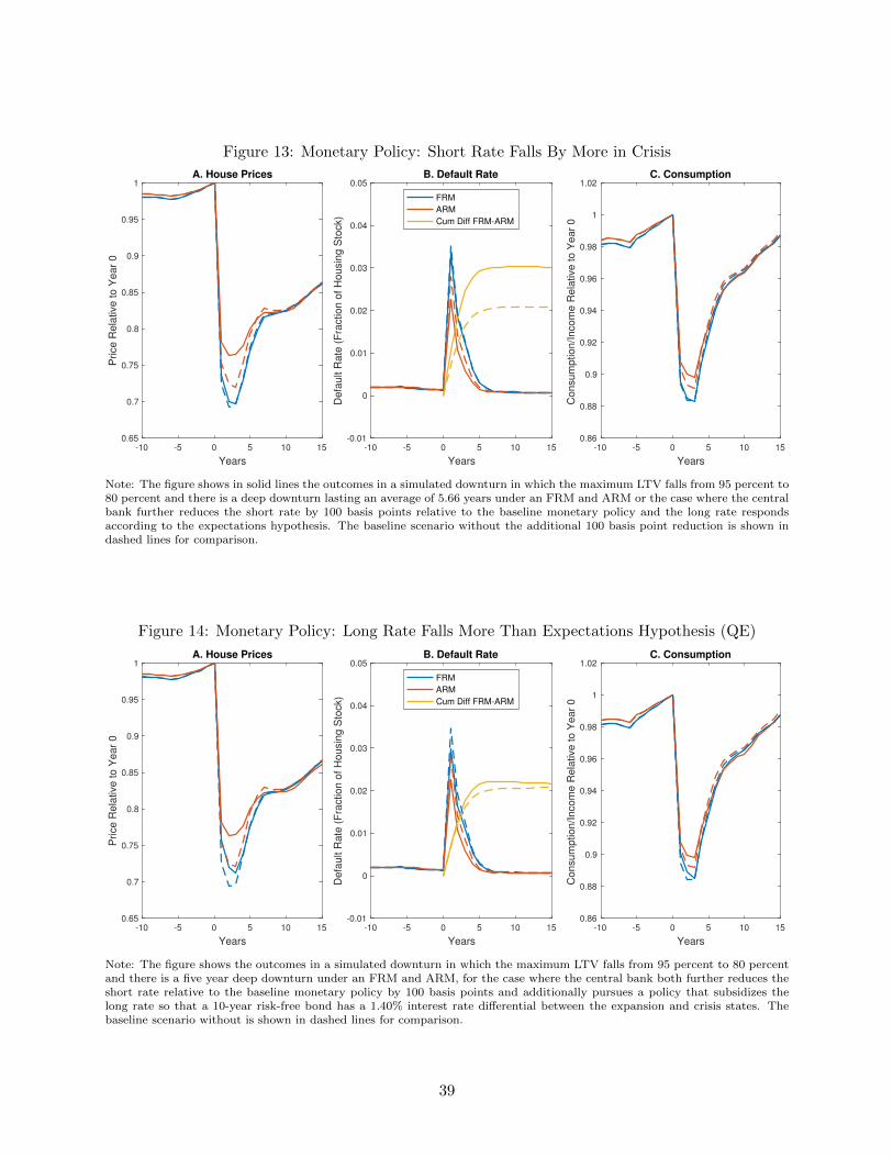
Figure 13: Monetary Policy: Short Rate Falls By More in Crisis

-10 -5 0 5 10 15

Years

0.65

0.7

0.75

0.8

0.85

0.9

0.95

1

Price

Re

lative

to

Ye

ar

0

A. House Prices

-10 -5 0 5 10 15

Years

-0.01

0

0.01

0.02

0.03

0.04

0.05

De

fau

lt R

ate

(F

ractio

n o

f H

ou

sin

g S

tock)

B. Default Rate

FRM

ARM

Cum Diff FRM-ARM

-10 -5 0 5 10 15

Years

0.86

0.88

0.9

0.92

0.94

0.96

0.98

1

1.02

Co

nsu

mp

tio

n/I

nco

me

Re

lative

to

Ye

ar

0

C. Consumption

Note: The figure shows in solid lines the outcomes in a simulated downturn in which the maximum LTV falls from 95 percent to80 percent and there is a deep downturn lasting an average of 5.66 years under an FRM and ARM or the case where the centralbank further reduces the short rate by 100 basis points relative to the baseline monetary policy and the long rate respondsaccording to the expectations hypothesis. The baseline scenario without the additional 100 basis point reduction is shown indashed lines for comparison.

Figure 14: Monetary Policy: Long Rate Falls More Than Expectations Hypothesis (QE)

-10 -5 0 5 10 15

Years

0.65

0.7

0.75

0.8

0.85

0.9

0.95

1

Price

Re

lative

to

Ye

ar

0

A. House Prices

-10 -5 0 5 10 15

Years

-0.01

0

0.01

0.02

0.03

0.04

0.05

De

fau

lt R

ate

(F

ractio

n o

f H

ou

sin

g S

tock)

B. Default Rate

FRM

ARM

Cum Diff FRM-ARM

-10 -5 0 5 10 15

Years

0.86

0.88

0.9

0.92

0.94

0.96

0.98

1

1.02

Co

nsu

mp

tio

n/I

nco

me

Re

lative

to

Ye

ar

0

C. Consumption

Note: The figure shows the outcomes in a simulated downturn in which the maximum LTV falls from 95 percent to 80 percentand there is a five year deep downturn under an FRM and ARM, for the case where the central bank both further reduces theshort rate relative to the baseline monetary policy by 100 basis points and additionally pursues a policy that subsidizes thelong rate so that a 10-year risk-free bond has a 1.40% interest rate differential between the expansion and crisis states. Thebaseline scenario without is shown in dashed lines for comparison.

39

Figure 15: Monetary Policy: FRM With Underwater Refi Option With and Without QE

-10 -5 0 5 10 15

Years

0.65

0.7

0.75

0.8

0.85

0.9

0.95

1

Price

Re

lative

to

Ye

ar

0

A. House Prices

-10 -5 0 5 10 15

Years

0

0.005

0.01

0.015

0.02

0.025

0.03

0.035

0.04

0.045

0.05

De

fau

lt R

ate

(F

ractio

n o

f H

ou

sin

g S

tock)

B. Default Rate

FRMUR, Baseline

FRMUR, QE

Cumulative Diff

-10 -5 0 5 10 15

Years

0.86

0.88

0.9

0.92

0.94

0.96

0.98

1

1.02

Co

nsu

mp

tio

n/I

nco

me

Re

lative

to

Ye

ar

0

C. Consumption

Note: The figure shows the outcomes in a simulated downturn in which the maximum LTV falls from 95 percent to 80 percentand there is a five year deep downturn under an FRM with an underwater refinancing option for the baseline monetary policyand for the case where the central bank both further reduces the short rate relative to the baseline monetary policy by 100basis points and additionally pursues a policy that subsidizes the long rate so that a 10-year risk-free bond has a 1.40% interestrate differential between the expansion and crisis states.

because FRMs are priced off the long end of the yield curve. Since few households have liquid

assets and most saving in the economy is for retirement, housing demand by young households and

the behavior of high-LTV households that are primarily young is unchanged, and so the housing

market equilibrium is not substantially affected.

On the other hand, more aggressive monetary policy that affects short rates is useful when

homeowners have ARMs. Price declines and default are substantially lower and consumption is

slightly higher due to the more aggressive monetary policy. This is, of course, not surprising. Lower

short-rates leads to lower mortgage payments which leads to less default and a smaller price-default

spiral, and lower short rates also stimulate rental demand more. When aggressive monetary policy

in a crisis takes the form of subsidizing FRMs to the point that the risk-free 10-year long rate

falls 1.4 percent in the crisis relative to an expansion, the FRM economy looks much better than

under the baseline monetary policy, as shown in Figure 14. Prices fall by 1.8 percentage points less

than with FRM under the baseline monetary policy, and 6.9 percent of the housing stock defaults

over eight years. Relative to the baseline monetary policy, welfare is improved by 0.43 percent of

annual consumption. These figures are an improvement but still fall short of the ARM under the

baseline monetary policy, which improves welfare by 0.83 percent of annual consumption relative

to the FRM. The mechanism behind these results, however, is quite different from the comparison

of ARM and FRM under the baseline monetary policy. The monetary policy is not passed through

to existing homeowners who cannot refinance at the lower rates. Indeed, many remain liquidity

constrained and the default rate is high. Instead, new homeowners can now lock in cheap financing,

which stimulates demand for housing and boosts house prices. Some exiting homeowners are no

longer bound by the LTV constraint and are able to refinance due to the rise in prices, undoing

40

some of the price-default spiral.

Our central finding about the added benefits of front-loading payment relief suggests that ex

post policies such as HARP, which setting aside implementation frictions are the same as FRM

with an underwater refinancing option, are maximally effective only if paired with policies to push

down long rates such as QE. To show this quantitatively, Figure 15 compares the FRM with

underwater refinancing under the baseline policy and the more aggressive short rate policy coupled

with quantitative easing to generate a 1.4 percent drop in the risk-free 10-year long rate – and thus

a 1.4 percent decline in the FRM rate for homeowners who exercise their refinancing option that

is tied to this rate – in the crisis. One can see that the benefits of the FRM with an underwater

refinancing option are stronger for prices, default, and consumption when coupled with QE. Prices

fall by 2.15 percentage points less than the baseline policy, consumption falls 0.23 percentage points

less, and the default rate is 5.90 percent over eight years rather than 7.32 percent. Consumption

equivalent welfare rises by the equivalent of 0.52 percent of annual consumption relative to the

baseline monetary policy. Compared to the FRM under the quantitative easing policy, welfare rises

the equivalent of 0.29 percent of annual consumption. Still, FRMUR with quantitative easing is not

an improvement relative to ARM or EK under the baseline policy, and certainly not an improvement

relative to ARM with the more aggressive monetary policy in the crisis. This suggests that even

setting aside the costs of unconventional monetary policy, many of its benefits can be achieved

more directly through mortgage design coupled with conventional monetary policy.

8 Conclusion

We assess how mortgages can be redesigned or modified in a crisis to reduce housing market

volatility, consumption volatility, and default and how mortgage design interacts with monetary

policy. To do so, we construct a quantitative equilibrium life cycle model with aggregate shocks in

which households have realistic long-term mortgages that are priced by risk-neutral and competitive

lenders and household decisions aggregate up to determine house prices. We calibrate the model to

match aggregate moments as well as quasi-experimental evidence on the effect of payment size and

LTV on default so that our model is tailored to qualitatively assess the benefits of adding simple

state contingency to mortgage contracts.

We use the model to assess the performance of various mortgage contracts in a realistic,

recession-driven housing crisis. In our model, indexing payments to monetary policy significantly

reduces household consumption volatility and default. If the central bank reduces interest rates in

response to the crisis, mortgage payments fall both by more and regardless of whether a household

refinances, which helps to smooth consumption, limits default by relaxing budget constraints in

bad states, and stimulates housing demand by new homeowners. These hedging benefits are quite

large for constrained, high LTV households who bear the brunt of the housing bust. The over-

all welfare benefit to the economy of switching to ARMs is equivalent to 0.83 percent of annual

consumption. Crucially, these benefits depend on the extent to which the insurance provided by

ARMs is anticipated by households, as households take on more debt and hold fewer liquid assets

when they expect their payments to fall in a crisis, leading to more macro fragility.

41

Our main conclusion is that mortgages that front-load payment relief provide much better

outcomes for households and can substantially improve household welfare. Reducing monthly

payments in a crisis alleviates liquidity constraints when they are most binding, limits default, and

stimulates housing demand by renters, which stems house price declines and ameliorates pecuniary

externalities that work through the price of housing. The clearest example of the benefits of front-

loading payment reductions comes from our comparison of a FRM with an option to convert to

an an ARM to an FRM with an option to refinance underwater. Although both mortgages have

similar effects on the balance sheets of lenders when a crisis hits due to the expectations hypothesis,

the EK convertible mortgage front-loads payment reductions during the crisis, increases welfare by

four times as much, and reduces defaults by three times as much as the FRMUR. The FRMUR

does worse because it is priced off the long end of the yield curve and thus smooths payment relief

over the life of the loan, providing households payment relief in states where they need it less.

While the comparison of these two loans gives the starkest contrast, there are a number of

different ways in which one might front-load payment relief. We consider quantitatively the option

ARM, which allows households to insure idiosyncratic shocks. One might also consider an ARM

with a cap or an FRM or ARM that can have its payments cut in a recession through term extension.

We leave the analysis of the best way to front-load payment relief for future research.

42

References

Agarwal, S., G. Amromin, I. Ben-David, S. Chomsisengphet, T. Piskorski, and A. Seru (2017).

Policy Intervention in Debt Renegotiation: Evidence from the Home Affordable Modification

Program. Journal of Political Economy 125 (3), 654–712.

Agarwal, S., G. Amromin, S. Chomsisengphet, T. Landvoigt, T. Piskorski, A. Seru, and V. Yao

(2017). Mortgage Refinancing, Consumer Spending, and Competition: Evidence from the

Home Affordable Refinancing Program.

Andersson, F. and T. Mayock (2014). Loss Severities on Residential Real Estate during the Great

Recession. Journal of Banking and Finance 46, 266–284.

Auclert, A. (2017). Monetary Policy and the Redistribution Channel.

Beraja, M., A. Fuster, E. Hurst, and J. Vavra (2017). Regional Heterogeneity and Monetary

Policy.

Bhutta, N., J. Dokko, and H. Shan (2017). Consumer Ruthlessness and Mortgage Default During

the 2007 to 2009 Housing Bust. Journal of Finance 72 (6), 2433–2466.

Brueckner, J. K. and K. Lee (2017). Optimal Sharing of Interest-Rate Risk in Mortgage Con-

tracts: The Effects of Pontential Prepayment and Default. Real Estate Economics.

Calza, A., L. Stracca, and T. Monacelli (2013). Housing Finance and Monetary Policy. Journal

of the European Economic Association 11 (S1), 101–122.

Campbell, J. Y. (2013). Mortgage Market Design. Review of Finance 17 (1), 1–33.

Campbell, J. Y. and J. F. Cocco (2003). Household Risk Management and Optimal Mortgage

Choice. Quarterly Journal of Economics 118 (4), 1449–1494.

Campbell, J. Y. and J. F. Cocco (2015). A Model of Mortgage Default. The Journal of Fi-

nance 70 (4), 1495–1554.

Campbell, J. Y., S. Giglio, and P. Pathak (2011). Forced Sales and House Prices. American

Economic Review 101 (5), 2108–31.

Caplin, A., C. Freeman, and J. Tracy (1997). Collateral Damage: Refinancing Constraints and

Regional Recessions. Journal of Money, Credit, and Banking 29 (4), 496–516.

Cloyne, J., C. Ferreira, and P. Surico (2017). Monetary Policy When Households Have Debt:

New Evidence on the Transmission Mechanism.

Corbae, D. and E. Quintin (2015). Leverage and the Foreclosure Crisis. Journal of Political

Economy 123 (1), 1–65.

Den Haan, W. J. (2010). Assessing the Accuracy of the Aggregate Law of Motion in Models

With Heterogenous Agents. Journal of Economic Dynamics and Control 34 (1), 79–99.

Di Maggio, M., A. Kermani, B. J. Keys, T. Piskorski, R. Ramcharan, A. Seru, and V. Yao

(2017). Monetary Policy Pass-Through: Household Consumption and Voluntary Deleverag-

ing. American Economic Review 107 (11), 3550–3588.

43

Eberly, J. and A. Krishnamurthy (2014). Efficient credit policies in a housing debt crisis. Brook-

ings Papers on Economic Activity , 73–136.

Elul, R., N. S. Souleles, S. Chomsisengphet, D. Glennon, and R. Hunt (2010). What ’Triggers’

Mortgage Default? American Economic Review 100 (2), 490–4.

Farmer, L. and A. A. Toda (2017). Discretizing Nonlinear, Non-Gaussian Markov Processes with

Exact Conditional Moments. Quantitative Economics 8 (2), 651–683.

Favilukis, J., S. C. Ludvigson, and S. Van Nieuwerburgh (2017). The Macroeconomic Effects of

Housing Wealth, Housing Finance, and Limited Risk-Sharing in General Equilibrium. Journal

of Political Economy 125 (1), 140–223.

Floden, M. and J. Linde (2001). Idiosyncratic Risk in the United States and Sweden: Is There

a Role for Government Insurance? Review of Economic Dynamics 4, 406–437.

Foote, C. L., K. Gerardi, and P. S. Willen (2008). Negative Equity and Foreclosure: Theory and

Evidence. Journal of Urban Economics 64 (2), 234–245.

Fuster, A. and P. S. Willen (2017). Payment Size, Negative Equity, and Mortgage Default.

American Economic Journal: Economic Policy 9 (4), 167–191.

Ganong, P. and P. Noel (2017). The Effect of Debt on Default and Consumption: Evidence from

Housing Policy in the Great Recession.

Garriga, C., F. E. Kydland, and R. Sustek (2016). Nominal Rigidities in Debt and Product

Markets. NBER Working Paper Series, 1–52.

Glaeser, E. L. and J. Gyourko (2005). Urban Decline and Durable Housing. Journal of Political

Economy 113 (2), 345–375.

Glaeser, E. L. and J. Gyourko (2009). Arbitrage in Housing Markets. In E. L. Glaeser and

J. M. Quigley (Eds.), Housing Markets and the Economy: Risk, Regulation, and Policy, pp.

113–148. Cambridge, MA: Lincoln Institute of Land Policy.

Greenwald, D. L. (2017). The Mortgage Credit Channel of Macroeconomic Transmission.

Greenwald, D. L., T. Landvoigt, and S. Van Nieuwerburgh (2017). Finanical Fragility With

SAM?

Guren, A. (2018). House Price Momentum and Strategic Complementarity.

Guren, A. and T. McQuade (2018). How Do Foreclosures Exacerbate Housing Downturns?

Guvenen, F. and J. Anthony A. Smith (2014). Inferring Labor Income Risk and Partial Insurance

From Economic Choices. Econometrica 82 (6), 2085–2129.

Guvenen, F., F. Karahan, S. Ozkan, and J. Song (2016). What Do Data on Millions of U.S.

Workers Reveal about Life-Cycle Earnings Dynamics?

Guvenen, F., S. Ozkan, and J. Song (2014). The Nature of Countercyclical Income Risk. Journal

of Political Economy 122 (3), 621–660.

Halket, J., L. Nesheim, and F. Oswald (2017). The Housing Stock, House Prices, and User Costs:

The Roles of Location, Structure, and Unobserved Quality.

44

Heathcote, J., K. Storesletten, and G. Violante (2017). Optimal Tax Progressivity: An Analytical

Framework. Quarterly Journal of Economics.

Hurst, E., B. J. Keys, A. Seru, and J. Vavra (2016). Regional Redistribution through the US

Mortgage Market. American Economic Review 106 (10), 2982–3028.

Justiniano, A., G. E. Primiceri, and A. Tambalotti (2017). Credit supply and the housing boom.

Kaplan, G., K. Mitman, and G. L. Violante (2017). The Housing Boom and Bust: Model Meets

Evidence.

Krueger, D., K. Mitman, and F. Perri (2016). On the Distribution of the Welfare Losses of Large

Recession. In B. Honore, A. Pakes, M. Piazzesi, and L. Samuelson (Eds.), Advances in Eco-

nomics and Econometrics: Theory and Applications, Eleventh World Congress. Cambridge,

UK: Cambridge University Press.

Krusell, P. and J. Anthony A. Smith (1998). Income and Wealth Heterogeneity in the Macroe-

conomy. Journal of Political Economy 106 (5), 867–896.

Kung, E. (2015). Mortgage Market Institutions and Housing Market Outcomes.

Li, W. and R. Yao (2007). The Life-Cycle Effects of House Price Changes. Journal of Money,

Credit and Banking 39 (6), 1375–1409.

Lucas, D., M. Remy, and D. Moore (2011). An Evaluation of Large-Scale Mortgage Refinancing

Programs.

Mian, A., K. Rao, and A. Sufi (2013). Household Balance Sheets, Consumption, and the Ecoomic

Slump. Quarterly Journal of Economics 128, 1687–1726.

Mian, A. and A. Sufi (2011). House Prices, Home Equity-Based Borrowing, and the U.S. House-

hold Leverage Crisis. American Economic Review 101 (5), 2132–2156.

Mian, A., A. Sufi, and F. Trebbi (2015). Foreclosures, House Prices, and the Real Economy.

Journal of Finance 70 (6), 2587–2634.

Piskorski, T. and A. Seru (2018). Mortgage Market Design: Lessons From the Great Recession.

Piskorski, T. and A. Tchistyi (2010). Optimal Mortgage Design. Review of Financial Stud-

ies 23 (8), 3098–3140.

Piskorski, T. and A. Tchistyi (2011). Stochastic House Appreciation and Optimal Mortgage

Lending. Review of Financial Studies 24 (5), 1407–1446.

Piskorski, T. and A. Tchistyi (2017). An Equilibrium Model of Housing and Mortgage Marekts

With State-Contingent Lending Contracts.

Wong, A. (2018). Population Aging and the Transmission of Monetary Policy to Consumption.

45

A Numerical Implementation

We solve the model numerically by discretizing the state space. Because the aggregate state Θt has

five values, we use five values for the interest rate. We use seven grid points for income. We use 22

grid points for savings, with a denser grid at low savings. We use 41 grid points for the mortgage

balance, with two balances for renters (with and without the default flag), and 39 values for the

mortgage including zero. The grid is denser for higher balances that are close to the equilibrium

price given that amortization schedules feature smaller principal payments earlier in the mortgage.

Finally, we use eight equally-spaced grid points for the house price and interpolate on the price grid

when the price falls between grid points. We have experimented with finer grids and have found

the results are not sensitive to the grids we choose.

We solve the household’s problem by backward induction, starting with an initial guess for the

mortgage spreads and the forecast rules. We then simulate 19,000 years of data and throw out

the first 100 years. In each period of the simulation, a new generation is born and shocks hit the

economy. We then calculate the supply and demand schedules, calculate the equilibrium price,

and finally update the distribution of individuals across states according to the policy functions,

interpolating between price grid points.

We then follow the Krusell and Smith-style algorithm described in the main text. We run

forecast rule regressions:

log pt+1 = f(Θt,Θt+1) (log pt)

where f(Θt,Θt+1) is a function for each realization of (Θt,Θt+1). Because Θt has five values, there

are potentially 25 forecast rules, but 12 relate to (Θt,Θt+1) transitions that do not occur in practice

(e.g., one only transitions to the tight credit state after a crisis) so there are only 13 forecast rules

that must converge. We parameterize f (·) as a linear spline with knot points located at the price

grid points. After running the regressions on the simulated data, we update the forecast rules

to a convex combination of the original forecast rules and the regressions.32 We also solve for the

equilibrium spreads given κ and update the spreads to a convex combination of the original forecast

spreads and the new zero profit spreads. We iterate until the forecast rules and spreads converge.

Three criteria must be simultaneously met for convergence. First, the spread must be within one

basis point of the actual break-even spread. Second, the forecast rule R-squareds must converge so

that the difference is less than 0.0025 between iterations. Third, for all forecast rules, the distance

between the regression and the forecast rule must be less than 0.005 at all prices for which we

observe data in our 19,000-period simulation. In practice, the third criterion is the most stringent,

and our spreads and forecast rules are highly accurate as described below.

For the FRM in the baseline calibration, we must solve for the κ that implies that the average

spread between the spread in the model and a 10-year bond is 1.65 percent as in the data. For this,

we follow a similar algorithm to the one described above, but in addition to adjusting the spread

and forecast rules, we adjust κ to hit the 1.65 percent average spread between the 10 year mortgage

and a synthetic 10-year bond rate calculated by the expectations hypothesis. κ converges along

32One could in principle simply use the regression as the new forecast rule, but we have found that this leads tooscillating behavior. We consequently use a convex combination which, while slower, provides better convergenceproperties.

46

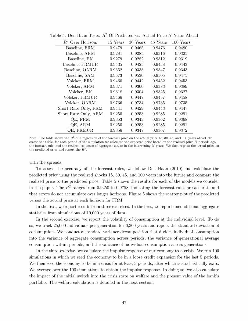
Table 5: Den Haan Tests: R2 Of Predicted vs. Actual Price N Years Ahead

R2 Over Horizon: 15 Years 30 Years 45 Years 100 Years

Baseline, FRM 0.9479 0.9465 0.9476 0.9480Baseline, ARM 0.9281 0.9285 0.9316 0.9325Baseline, EK 0.9279 0.9282 0.9312 0.9319

Baseline, FRMUR 0.9435 0.9425 0.9438 0.9443Baseline, OARM 0.9352 0.9338 0.9347 0.9343Baseline, SAM 0.9573 0.9530 0.9505 0.9475Volcker, FRM 0.9460 0.9442 0.9452 0.9453Volcker, ARM 0.9371 0.9360 0.9383 0.9389Volcker, EK 0.9318 0.9304 0.9325 0.9327

Volcker, FRMUR 0.9466 0.9447 0.9457 0.9458Volcker, OARM 0.9736 0.9734 0.9735 0.9735

Short Rate Only, FRM 0.9441 0.9429 0.9443 0.9447Short Rate Only, ARM 0.9250 0.9253 0.9285 0.9291

QE, FRM 0.9353 0.9343 0.9362 0.9368QE, ARM 0.9250 0.9253 0.9285 0.9291

QE, FRMUR 0.9356 0.9347 0.9367 0.9372

Note: The table shows the R2 of a regression of the forecast price on the actual price 15, 30, 45, and 100 years ahead. Tocreate the table, for each period of the simulation we calculate the expected price based on the realized price N periods ago,the forecast rule, and the realized sequence of aggregate states in the intervening N years. We then regress the actual price onthe predicted price and report the R2.

with the spreads.

To assess the accuracy of the forecast rules, we follow Den Haan (2010) and calculate the

predicted price using the realized shocks 15, 30, 45, and 100 years into the future and compare the

realized price to the predicted price. Table 5 shows the results for each of the models we consider

in the paper. The R2 ranges from 0.9250 to 0.9758, indicating the forecast rules are accurate and

that errors do not accumulate over longer horizons. Figure 5 shows the scatter plot of the predicted

versus the actual price at each horizon for FRM.

In the text, we report results from three exercises. In the first, we report unconditional aggregate

statistics from simulations of 19,000 years of data.

In the second exercise, we report the volatility of consumption at the individual level. To do

so, we track 25,000 individuals per generation for 6,300 years and report the standard deviation of

consumption. We conduct a standard variance decomposition that divides individual consumption

into the variance of aggregate consumption across periods, the variance of generational average

consumption within periods, and the variance of individual consumption across generations.

In the third exercise, we calculate the impulse response of our economy to a crisis. We run 100

simulations in which we seed the economy to be in a loose credit expansion for the last 5 periods.

We then seed the economy to be in a crisis for at least 3 periods, after which is stochastically exits.

We average over the 100 simulations to obtain the impulse response. In doing so, we also calculate

the impact of the initial switch into the crisis state on welfare and the present value of the bank’s

portfolio. The welfare calculation is detailed in the next section.

47

Figure 16: Den Haan Tests: Scatter Of Predicted vs. Actual Price N Years Ahead For FRM

3 4 5 6

Price

3

3.5

4

4.5

5

5.5

6

Pre

dic

ted

Price

Price vs. Den Haan 15 year Prediction

3 4 5 6

Price

3

3.5

4

4.5

5

5.5

6

Pre

dic

ted

Price

Price vs. Den Haan 30 year Prediction

3 4 5 6

Price

3

3.5

4

4.5

5

5.5

6

Pre

dic

ted

Price

Price vs. Den Haan 45 year Prediction

3 4 5 6

Price

3

3.5

4

4.5

5

5.5

6

Pre

dic

ted

Price

Price vs. Den Haan 100 year Prediction

Note: The figure shows a scatter plot of the forecast price 15, 30, 45, and 100 years ahead versus the actual price. To createthe figure, for each period of the simulation we calculate the expected price based on the realized price N periods ago, theforecast rule, and the realized sequence of aggregate states in the intervening N years.

B Welfare

The value function in our model for an age a individual at time t in idiosyncratic state stj and

aggregate state Σt is:

V at

(sjt ,Σt

)= Et

T−a∑t=0

βt[c1−σt

1− σ+ αaHt − 1 [Defaultt] d

]+ βT−aψ

(b+ ξ)1−γ

1− γ

,

where ct is consumption at time t, b is the bequest at time T , Ht is housing at time t, and Defaultt

is an indicator for default at time t. Define the value function under two different economies 0 and

1 as V a,0t and V a,1

t .

We want to calculate the consumption-equivalent welfare change, which we denote by ∆a(sjt ,Σt

).

We calculate the welfare change as equivalent variation, that is the amount consumption would

have to increase by in economy 0 to make the agent indifferent between economy 0 and economy

48

1. ∆a(sjt ,Σt

)is thus defined implicitly as:

V a,1t

(sjtΣt

)= Et

T−a∑t=0

βt

(c0t

(1 + ∆a

(sjt ,Σt

)))1−σ

1− σ+ αH0

t − 1[Default0t

]d

+ βT−aψ

(b0 + ξ

)1−γ1− γ

= V a,0

t

(sjt ,Σt

)+

[(1 + ∆a

(sjt ,Σt

))1−σ− 1

]Et

T−a∑t=0

βt

[(c0t

)1−σ1− σ

].

Consequently,

∆a(sjt ,Σt

)=

1 +V a,1t

(sjt ,Σt

)− V a,0

t

(sjt ,Σt

)Et

∑T−at=0 βt

[(c0t )

1−σ

1−σ

]

11−σ

− 1.

We report two distinct welfare calculations. The first is the unconditional welfare. This is

defined as the consumption-equivalent equivalent variation of being born in economy 0 relative to

economy 1. Because we are using equivalent variation, we use the ergodic distribution for the initial

generation over both micro and macro states in the 0 economy, which we denote by ω0, to weight

the value functions in the 0 economy and the 1 economy. The aggregate unconditional welfare

difference between economies 0 and 1 is then:

∆ =

∫∆a(sjt ,Σt

)dω0.

The second welfare calculation is the aggregate welfare loss experienced when the economy

switches from a loose-credit expansion to the crisis state. We follow Krueger et al. (2016) in

calculating the welfare losses from a switch in the aggregate state as “the permanent percentage

increase in consumption that a...household would require so that its welfare in the transition is

the same as the welfare when the transition does not happen.” Given this, we can define the

consumption-equivalent equivalent variation welfare change for a household with idiosyncratic state

sjt of going from aggregate state Σ0t to aggregate state Σ1

t as:

∆aΣ0tΣ

1t

(sjt

)=

1 +V at

(sjt ,Σ

1t

)− V a

t

(sjt ,Σ

0t

)Et

∑T−at=0 βt

[(c0t )

1−σ

1−σ

]

11−σ

− 1.

For aggregate welfare, the concept we use is also from Krueger et al.: “Suppose households are

randomly placed into the pre-recession cross-sectional distribution over individual characteristics.

Under the veil of ignorance of not knowing where in the distribution one would be placed, we ask by

what percentage would lifetime consumption of everyone need to be increased to be compensated

from the loss of falling into a recession.” Define Ωat as the distribution of households of age a across

states at the beginning of period t, when the shock hits. Consumption equivalent welfare for age a

49

is then:

∆aΣ0tΣ

1t

=

∫∆a

Σ0t ,Σ

1tdΩa

t

We aggregate across generations living when the switch in aggregate states occurs to compute

∆Σ0tΣ

1t

for each mortgage type. This calculation does not include the effect of the crisis on new

generations. Rather than reporting ∆Σ0tΣ

1t

directly, we report the difference between ∆Σ0tΣ

1t

under

FRM and ∆Σ0tΣ

1t

for alternative mortgage designs.

C Calibration Details

C.1 Income Process

This appendix details the calibration of the income process.

Our first task is to create a discretized income process with left skewness in busts. We assume

that the income process of Floden and Linde (2001) holds in an expansion and add left skewness

in a recession to match the left skewness observed in 2008-9 by Guvenen et al. (2014). We then

discretize the resulting distribution using the method of Farmer and Today (2017) modified slightly

to discretize two idiosyncratic shock distributions on the same grid. Because there are multiple

ways to add this amount of left skewness, we need an additional moment to match. In particular, we

match the standard deviation of aggregate log income of 0.0215. Finally, we adjust the distribution

of initial income for incoming distributions to best match the lifecycle profile of income in Guvenen

et al. (2016) and adjust the aggregate income level so that we obtain an average income of one.

We now describe how we implement this procedure in detail. Our first step is to create a

mixture of normals to target in the Farmer and Toda (2017) procedure. We assume that the

distribution of idiosyncratic shocks is the same in expansions regardless of whether credit is loose

or tight. Similarly, the distribution of idiosyncratic shock is the same in recessions and crises, again

regardless of whether credit is loose or tight. In expansions, we use the income process of Floden

and Linde (2001), which is an AR(1) process with a standard deviation of 0.21 log points and an

annual persistence of 0.91. In a crisis or recession, we add the standardized skewness of the 2008-9

income change distribution from Guvenen et al. (2014) to the mixture of normals. To do this, we

fit a mixture of normals to the histogram underlying Figure 12 in Guvenen et al. (2014). We then

calculate the standardized skewness of this distribution. We then adjust the Floden and Linde

(2001) income process by adding mass to the left tail to match the same standardized skewness we

found in the Guvenen et al. data.

With these mixtures of normals in hand, we then adjust three parameters to target three

moments: the standard deviation of aggregate log income, the fit between the model and data age-

income profiles, and an aggregate income of one. We adjust three parameters in a minimum distance

routine. First, we shift the mean of the bust idiosyncratic shock distribution, which allows us to

target the standard deviation of log income in the data. Second, we adjust fraction of the population

that starts at each initial income which allows us to target the age-income profile. Third, we adjust

the level of the aggregate income vector yagg, which allows us to target an average income of one.

For each vector of parameters, we apply a modified version of the Farmer and Toda (2017) algorithm

50

using code from Toda’s website. The modification is to calculate the idiosyncratic income grid using

only the boom distribution and then discretizing both the boom and bust distributions on the same

grid. Given the left skewness, we use a grid with grid-points spaced from 2.5 standard deviations

below the mean to 1.5 standard deviations above the mean. After discretizing, we simulate income,

generate simulated data and calculate the average aggregate income, the standard deviation of log

income, and the mean squared error between the age-income profile in the data and the model, and

then search over the parameter space to find the optimal. We match the standard deviation of log

income and aggregate income nearly exactly, and the fit to the age-income profile is close as shown

in Figure 17.

We obtain from this calibration procedure four objects objects: a transition matrix that is a

function of the aggregate state Ξid (Θt), a vector yagg (Θt) which gives log aggregate income as a

function of the aggregate state, a log idiosyncratic income vector yid for non-retirement (and im-

plicitly a log idiosyncratic income vector for retirement that is equal to yid−0.35 by our assumption

of a 0.35 log point income decline in retirement), and an entrant distribution over the idiosyncratic

states. Recall that we discretize to seven idiosyncratic incomes and have five aggregate states. For

these vectors and matrices, we let state 1 be the crisis, state 2 be a recession with loose credit,

state 3 be an expansion with loose credit, state 4 be a recession with tight credit, and state 5 be

an expansion with tight credit.

The aggregate income vector is

yagg =

0.0976

0.1426

0.1776

0.1426

0.1776

We calibrate so that aggregate income falls by 8.0 percent in a crisis and 3.5 percent in a recession,

so this is just a normalization of the resulting vector ensuring that aggregate income is on average

equal to one.

The idiosyncratic income vector is:

yid =

−1.2663

−0.9286

−0.5909

−0.2533

0.0844

0.4221

0.7598

The distribution of entrants has 92.69 percent weight on the second to bottom grid point and 7.31

percent weight on the third to bottom grid point.

By assumption, the idiosyncratic income distribution is the same in the crisis state, the recession

51

Figure 17: Age-Income Profile in Model and Data

25 30 35 40 45 50 55 60 65 70

Age

-0.6

-0.5

-0.4

-0.3

-0.2

-0.1

0

0.1

0.2

0.3

Log P

oin

ts

Lifecycle Profile of Average Log Income Rel to Mean

Model

Data

Note: This figure shows the age-income distribution. The x axis is ages from 26 to 70 in our model. The y axis shows averagelog income by age, with zero being the average log income in the model. The data come from Guvenen et al. (2016). Theretirement data is equal to the average income at 60 minus 0.35 to be consistent with retirement in our model. The model issimulated from our model.

state with loose credit, and the recession state with tight credit. It is equal to:

Ξid (Crisis or Recession) =

0.8183 0.1593 0.0103 0.0003 0.0001 0.0001 0.0116

0.1820 0.5046 0.2847 0.0279 0.0007 0.0001 0

0.0563 0.0783 0.6038 0.2611 0.0005 0 0

0.0123 0.0209 0.1493 0.6123 0.2011 0.0041 0

0.0021 0.0091 0.0227 0.1939 0.6093 0.1595 0.0034

0.0001 0.0019 0.0099 0.0268 0.2391 0.5904 0.1318

0.0033 0.0049 0.0067 0.0083 0.0140 0.1648 0.7980

In this matrix, the probability listed is the probability of a transition from the row i to the column

j, so that rows add to a probability of one. By assumption, the idiosyncratic income distribution

is the same in the expansion state regardless of the state of credit and is equal to:

Ξid (Expandsion) =

0.7059 0.2663 0.0235 0.0005 0 0 0.0038

0.0911 0.5794 0.3204 0.0091 0 0 0

0.0021 0.1138 0.6156 0.26116 0.0069 0 0

0 0.0030 0.1478 0.6327 0.2116 0.0049 0

0 0 0.0042 0.1887 0.6361 0.1674 0.0036

0 0 0 0.0032 0.2462 0.6104 0.1402

0.0070 0 0 0.0001 0.0073 0.1456 0.8400

.

Our calibration procedure does a good job of replicating key facts in the data that we target.

Figure 17 shows the age-income distribution in the model relative to the data. We impose on the

data that income falls 0.35 log points at retirement, so the retirement numbers are equal to average

income at 60 minus 0.35. The model does a good job of capturing the age-income profile at younger

ages. Figure 18 shows the distribution of idiosyncratic income shocks in the boom relative to the

bust. Our income shocks capture well the left skewness found by Guvenen et al. (2014).

52

Figure 18: Distribution of Idiosyncratic Income Shocks in Boom vs. Bust

-1.5 -1 -0.5 0 0.5 1 1.5

Log Income Change

0

0.1

0.2

0.3

0.4

0.5

0.6

0.7

Pro

babili

ty

Idiosyncratic Shocks: Boom vs. Bust

Boom

Bust

Note: This figure shows the distribution of idiosyncratic income shocks in the boom and the bust calculated from modelsimulations. The results compare favorably to the evidence in Guvenen et al. (2014).

C.2 Calibration Targets and Procedure

Most of the external calibration targets are described in the main text. There are a few details

that we relegate to this appendix. First, although the transition matrix is described in the main

text, we do not detail it there. Letting state 1 be the crisis, state 2 be a recession with loose credit,

state 3 be an expansion with loose credit, state 4 be a recession with tight credit, and state 5 be

an expansion with tight credit, the transition matrix is:

ΞΘ =

0.6364 0 0 0 0.3636

0 0.1011 0.8989 0 0

0.0133 0.1832 0.8035 0 0

0 0 0 0.1011 0.8989

0.0133 0 0.0200 0.1832 0.7835

In this matrix, the probability listed is the probability of a transition from the row i to the column

j, so that rows add to one. The economy remains in the crisis state with a probability 63.64% of

the time and exits with a probability of 36.36%. The expansion and recession states look identical

for loose and tight credit except that in a tight-credit expansion the probability of remaining is

2% lower. There is a 2% probability the economy transitions to a loose credit expansion. The

economy enters a crisis from an expansion with 1.33% probability. The transition matrices between

expansion and recession are based on NBER dates as described in the main text.

The second detail relegated to the main text is how we reduce aa, the age-dependent valuation

of a house, in old age. We assume that this is constant at its calibrated value until retirement,

at which point it falls by 1/15 of its initial value each year until death, which is 10 years after

retirement. Our results are not sensitive to this specification.

We match four internal calibration targets. To match these four moments, we alter the param-

eters and solve the FRM economy under the baseline monetary policy. The average price is fairly

insensitive to ψ, ξ, and d and can be set using a alone, and we target a house price of five times

the average pre-tax income in the economy. We then alter ψ, ξ, and d to target three moments.

53

Table 6: Moments Matched in Calibration Procedure

Moment Data Model

Mean Price 5.00 5.010Ratio of Net Worth at 60 45 at 10th Percentile Net Worth 3.576 3.542

Ratio of Net Worth at 60 45 at Median Net Worth 2.096 2.092Cumulative Default Over 8 Year Crisis 8.0% 7.91%

Note: The four moments used in the calibration of a, ψ, ξ, and d. The model column indicates the moments in the model andthe data column indicates their values in the data that we use as targets.

Table 7: Downturn Moments For Various Mortgage Designs Under Volcker Monetary Policy

Design FRM ARM EK FRMUR Option ARM

Pct Point Reduction in Max ∆P Rel to FRM -1.83 0.04 0.00 -1.81Pct Point Reduction in Max ∆C Rel to FRM -0.67 -0.40 0.00 -0.60

Share Defaulting over 8 Years 10.3% 13.5% 10.9% 10.3% 15.6%Increase in Household Welfare Rel to FRM -0.72% -0.31% -0.01% -0.93%

Note: Table shows the indicated statistics for each mortgage design averaging across 100 simulations of a crisis that lasts 5.66years after an expansion with loose credit as described in the main text under the Volcker monetary policy. The top row showsthe percentage point change in the peak to trough change in price relative to FRM, with a positive number indicating a lesssevere price decline. The second row shows the percentage point change in the peak to trough change in consumption relativeto FRM, with a positive number indicating a less severe decline in consumption. The third row shows the share of the housingstock defaulting after 8 years. The fourth line shows the decline in household consumption-equivalent welfare relative to toFRM under the Volcker monetary policy reported as a percentage of annual consumption for the rest of the household’s life.

The first two are the ratio of total net worth at age 60 to age 45 in the SCF for the median and

10th percentile households by net worth. To smooth out noise in the SCF for any particular age,

we calculate total net worth at age 60 as the mean total net worth from ages 58 to 62 and total ent

worth at age 45 as the mean total net worth from age 43 to 47. We find a 10th percentile ratio of

3.576 in the SCF and a ratio at the median of 2.096. The final moment is the cumulative default

rate over a eight years in our main impulse response, which we choose to target eight percent. The

four moments are matched quite well, as indicated in Table 6.

D Additional Numerical Results

D.1 Downturn Moments for Alternate Monetary Policies

Table 3 in the main text summarizes the performance of the various mortgage designs we consider

under the baseline monetary policy. Table 7 reports the same statistics this for the Volcker monetary

policy, and Table 8 reports the same statistics this for the short rate reduction and the short rate

reduction with quantitative easing monetary policy.

D.2 Mortgage Spreads and Yield Curves

This section documents the equilibrium yield curves and mortgage spreads in our model.

We consider five main mortgage designs. The FRM has an interest rate that depends on the

aggregate state in which the mortgage is originated. The ARM has a spread over the short rate

54

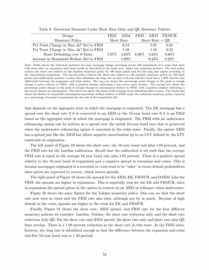
Table 8: Downturn Moments Under Short Rate Only and QE Monetary Policies

Design FRM ARM FRM ARM FRMURMonetary Policy Short Rate Short Rate + QE

Pct Point Change in Max ∆P Rel to FRM 6.54 5.07 0.68Pct Point Change in Max ∆C Rel to FRM 1.48 1.28 0.22

Share Defaulting over 8 Years 7.67% 4.63% 6.86% 4.63% 5.90%Increase in Household Welfare Rel to FRM 1.09% 0.43% 0.29%

Note: Table shows the indicated statistics for each mortgage design averaging across 100 simulations of a crisis that lasts5.66 years after an expansion with loose credit as described in the main text. under two monetary policies. The first policyreduces the short rate relative to the baseline monetary policy by 100 basis points and lets the long rate adjust according tothe expectations hypothesis. The second policy reduces the short rate relative to the baseline monetary policy by 100 basispoints and additionally pursues a policy that subsidizes the long rate so that a 10-year risk-free bond has a 1.40% interest ratedifferential between the expansion and crisis states. The top row shows the percentage point change in the peak to troughchange in price relative to FRM, with a positive number indicating a less severe price decline. The second row shows thepercentage point change in the peak to trough change in consumption relative to FRM, with a positive number indicating aless severe decline in consumption. The third row shows the share of the housing stock defaulting after 8 years. The fourth lineshows the decline in household consumption-equivalent welfare relative to FRM under the indicated monetary policy reportedas a percentage of annual consumption for the rest of the household’s life

that depends on the aggregate state in which the mortgage is originated. The EK mortgage has a

spread over the short rate if it is converted to an ARM or the 10-year bond rate if it is an FRM

based on the aggregate state in which the mortgage is originated. The FRM with an underwater

refinancing option can be written as a spread over the initial 10-year bond rate that is preserved

when the underwater refinancing option is exercised in the crisis state. Finally, the option ARM

has a spread just like the ARM but allows negative amortization up to an LTV defined by the LTV

constraint at origination.

The left panel of Figure 19 shows the short rate, the 10-year bond rate plus 1.65 percent, and

the FRM rate for the baseline calibration. Recall that the calibration is set such that the average

FRM rate is equal to the average 10 year bond rate plus 1.65 percent. There is a positive spread

relative to the 10-year bond in expansions and a negative spread in recessions and crises. This is

because mortgages originated in a recession or crisis tend to be “safer” in terms default probabilities

since prices are expected to recover, which lowers spreads.

The right panel of Figure 19 shows the spreads for the ARM, EK, FRMUR, and OARM. Like the

FRM, the spreads are higher in expansions. This is especially true for the EK and FRMUR, since

in expansions the spread prices in the option to convert to an ARM or refinance when underwater.

Figure 20 shows the same figures for the Volcker monetary policy. One can see that the short

rate now rises in crises and the FRM rate also rises, although not by as much. Because of high

default in the crisis, spreads are higher in the crisis for EK and FRMUR.

Finally, Figure 21 shows the short rate, ARM spread, and FRM rate for the four different

monetary policies we consider: baseline, Volcker, the short rate reduction only, and the short rate

reduction with QE. For the short rate and ARM spread, the short rate only and short rate plus QE

lines overlap. There is a 1.00 percent reduction in the short rate in this state. In the FRM rates,

however, the long rate is subsidized enough so that the difference between the expansion and crisis

risk-free 10-year bond rate is 1.40 percent.

55

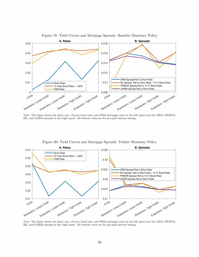
Figure 19: Yield Curves and Mortgage Spreads: Baseline Monetary Policy

Crisis

Recession, Loose C

redit

Expansion, Loose C

redit

Recession, Tight C

redit

Expansion, Tight C

redit

0

0.01

0.02

0.03

0.04

0.05A. Rates

Short Rate

10 Year Bond Rate + 1.65%

FRM Rate

Crisis

Recession, Loose C

redit

Expansion, Loose C

redit

Recession, Tight C

redit

Expansion, Tight C

redit

0.008

0.01

0.012

0.014

0.016

0.018B. Spreads

ARM Spread Rel to Short Rate

EK Spread Rel to Short Rate / 10 Yr Bond Rate

FRMUR Spread Rel to 10 Yr Bond Rate

OARM Spread Rel to Short Rate

Note: The figure shows the short rate, 10-year bond rate, and FRM mortgage rates in the left panel and the ARM, FRMUR,EK, and OARM spreads in the right panel. All interest rates are for pre-paid interest timing.

Figure 20: Yield Curves and Mortgage Spreads: Volcker Monetary Policy

Crisis

Recession, Loose C

redit

Expansion, Loose C

redit

Recession, Tight C

redit

Expansion, Tight C

redit

0.01

0.02

0.03

0.04

0.05

0.06

0.07A. Rates

Short Rate

10 Year Bond Rate + 1.65%

FRM Rate

Crisis

Recession, Loose C

redit

Expansion, Loose C

redit

Recession, Tight C

redit

Expansion, Tight C

redit

0.01

0.015

0.02

0.025

0.03

0.035B. Spreads

ARM Spread Rel to Short Rate

EK Spread Rel to Short Rate / 10 Yr Bond Rate

FRMUR Spread Rel to 10 Yr Bond Rate

OARM Spread Rel to Short Rate

Note: The figure shows the short rate, 10-year bond rate, and FRM mortgage rates in the left panel and the ARM, FRMUR,EK, and OARM spreads in the right panel. All interest rates are for pre-paid interest timing.

56

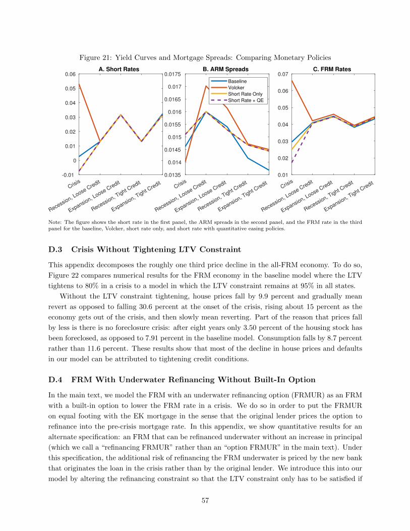
Figure 21: Yield Curves and Mortgage Spreads: Comparing Monetary Policies

Crisis

Recession, Loose C

redit

Expansion, Loose C

redit

Recession, Tight C

redit

Expansion, Tight C

redit

-0.01

0

0.01

0.02

0.03

0.04

0.05

0.06A. Short Rates

Crisis

Recession, Loose C

redit

Expansion, Loose C

redit

Recession, Tight C

redit

Expansion, Tight C

redit

0.0135

0.014

0.0145

0.015

0.0155

0.016

0.0165

0.017

0.0175B. ARM Spreads

Baseline

Volcker

Short Rate Only

Short Rate + QE

Crisis

Recession, Loose C

redit

Expansion, Loose C

redit

Recession, Tight C

redit

Expansion, Tight C

redit

0.01

0.02

0.03

0.04

0.05

0.06

0.07C. FRM Rates

Note: The figure shows the short rate in the first panel, the ARM spreads in the second panel, and the FRM rate in the thirdpanel for the baseline, Volcker, short rate only, and short rate with quantitative easing policies.

D.3 Crisis Without Tightening LTV Constraint

This appendix decomposes the roughly one third price decline in the all-FRM economy. To do so,

Figure 22 compares numerical results for the FRM economy in the baseline model where the LTV

tightens to 80% in a crisis to a model in which the LTV constraint remains at 95% in all states.

Without the LTV constraint tightening, house prices fall by 9.9 percent and gradually mean

revert as opposed to falling 30.6 percent at the onset of the crisis, rising about 15 percent as the

economy gets out of the crisis, and then slowly mean reverting. Part of the reason that prices fall

by less is there is no foreclosure crisis: after eight years only 3.50 percent of the housing stock has

been foreclosed, as opposed to 7.91 percent in the baseline model. Consumption falls by 8.7 percent

rather than 11.6 percent. These results show that most of the decline in house prices and defaults

in our model can be attributed to tightening credit conditions.

D.4 FRM With Underwater Refinancing Without Built-In Option

In the main text, we model the FRM with an underwater refinancing option (FRMUR) as an FRM

with a built-in option to lower the FRM rate in a crisis. We do so in order to put the FRMUR

on equal footing with the EK mortgage in the sense that the original lender prices the option to

refinance into the pre-crisis mortgage rate. In this appendix, we show quantitative results for an

alternate specification: an FRM that can be refinanced underwater without an increase in principal

(which we call a “refinancing FRMUR” rather than an “option FRMUR” in the main text). Under

this specification, the additional risk of refinancing the FRM underwater is priced by the new bank

that originates the loan in the crisis rather than by the original lender. We introduce this into our

model by altering the refinancing constraint so that the LTV constraint only has to be satisfied if

57

Figure 22: FRM vs. ARM: Housing Market Outcomes

-10 -5 0 5 10 15

Years

0.65

0.7

0.75

0.8

0.85

0.9

0.95

1

Price

Re

lative

to

Ye

ar

0

A. House Prices

-10 -5 0 5 10 15

Years

-0.01

0

0.01

0.02

0.03

0.04

0.05

De

fau

lt R

ate

(F

ractio

n o

f H

ou

sin

g S

tock)

B. Default Rate

FRM

No LTV Tightening

Cum Diff FRM-No LTV Tightening

-10 -5 0 5 10 15

Years

0.86

0.88

0.9

0.92

0.94

0.96

0.98

1

1.02

Co

nsu

mp

tio

n/I

nco

me

Re

lative

to

Ye

ar

0

C. Consumption

Note: The figure shows the impulse response to a simulated downturn preceded by an expansion with loose credit under FRM.In the LTV lightning case, the maximum LTV falls from 95 percent to 80 percent and the economy falls into a deep downturnfor an average of 5.66 years. In the case without LTV tightening, the maximum LTV stays at 95 percent but the same shockshit the economy and the monetary policy is unchanged.

the principal balance is being increased.

Figure 23 quantitatively compares the option FRMUR with the refinancing FRMUR. One can

see that the results are qualitatively and quantitatively similar, although the refinancing FRMUR

performs slightly more poorly than the option FRMUR. Indeed, the FRM that requires a refinancing

has a 0.6 percentage point larger decline in prices, has less initial default but more subsequent

default so that over eight years an additional 0.20 percent of homeowners default, and consumption

falls by 0.4 percentage points more. Consumption-equivalent welfare falls by 0.14 percent relative to

FRM for the refinancing FRMUR rather than rising 0.20 percent relative to FRM with the option

FRMUR. To understand the results, recall that with the option FRMUR, the option to refinance is

priced into the loan ex ante, which drives up the spread in expansion state. By contrast, with the

refinancing FRMUR, borrowers are allowed to refinance underwater and their default risk is priced

by the new lender that originates the refinanced loan in the crisis. These borrowers are riskier

because they have a high LTV, and this drives up the spread in the crisis state. Relative to the

option FRMUR, the gap between interest rates in the expansion and crisis state shrinks and the

amount of relief provided by the FRMUR is lower, leading to a slightly larger price decline, more

default, and lower welfare.

E Mortgage Amortization Schedule

In this appendix, we derive the amortization formula that defines the required minimum payment

for a mortgage in our setting with pre-paid interest.

Assume a mortgage is taken out with principal M0 at time 0 and amortizes over T periods at

58

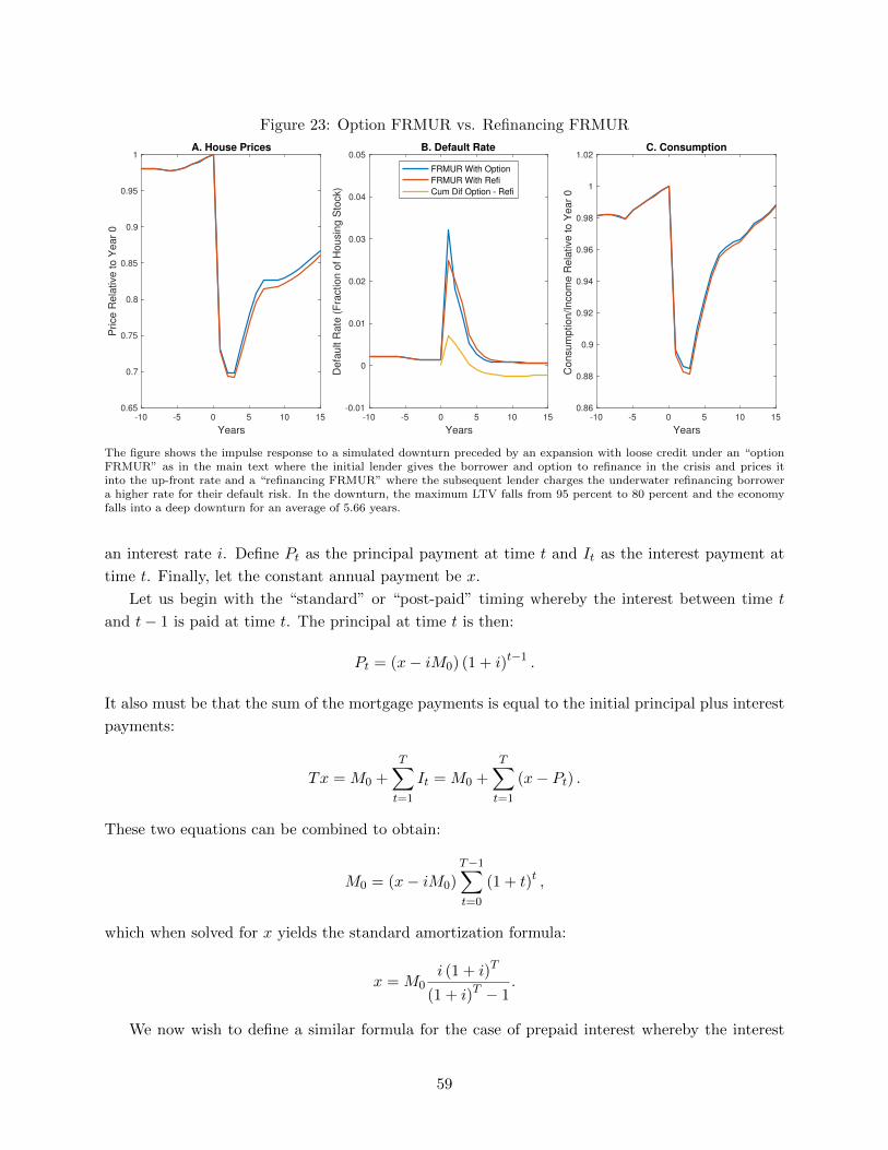
Figure 23: Option FRMUR vs. Refinancing FRMUR

-10 -5 0 5 10 15

Years

0.65

0.7

0.75

0.8

0.85

0.9

0.95

1

Price

Re

lative

to

Ye

ar

0

A. House Prices

-10 -5 0 5 10 15

Years

-0.01

0

0.01

0.02

0.03

0.04

0.05

De

fau

lt R

ate

(F

ractio

n o

f H

ou

sin

g S

tock)

B. Default Rate

FRMUR With Option

FRMUR With Refi

Cum Dif Option - Refi

-10 -5 0 5 10 15

Years

0.86

0.88

0.9

0.92

0.94

0.96

0.98

1

1.02

Co

nsu

mp

tio

n/I

nco

me

Re

lative

to

Ye

ar

0

C. Consumption

The figure shows the impulse response to a simulated downturn preceded by an expansion with loose credit under an “optionFRMUR” as in the main text where the initial lender gives the borrower and option to refinance in the crisis and prices itinto the up-front rate and a “refinancing FRMUR” where the subsequent lender charges the underwater refinancing borrowera higher rate for their default risk. In the downturn, the maximum LTV falls from 95 percent to 80 percent and the economyfalls into a deep downturn for an average of 5.66 years.

an interest rate i. Define Pt as the principal payment at time t and It as the interest payment at

time t. Finally, let the constant annual payment be x.

Let us begin with the “standard” or “post-paid” timing whereby the interest between time t

and t− 1 is paid at time t. The principal at time t is then:

Pt = (x− iM0) (1 + i)t−1 .

It also must be that the sum of the mortgage payments is equal to the initial principal plus interest

payments:

Tx = M0 +T∑t=1

It = M0 +T∑t=1

(x− Pt) .

These two equations can be combined to obtain:

M0 = (x− iM0)

T−1∑t=0

(1 + t)t ,

which when solved for x yields the standard amortization formula:

x = M0i (1 + i)T

(1 + i)T − 1.

We now wish to define a similar formula for the case of prepaid interest whereby the interest

59

between time t and t+1 is paid at t. To maintain symmetry with the standard formula, we assume

that the household takes out a mortgage of size M0 and in period one makes an interest payment

of iM0 + P0. As above, x = Pt + It but now IT = 0 and x = PT . Consequently:

Pt =(x− iM0)

(1 + i

1−i

)t1− i

and

Tx = M0 +T−1∑t=0

It = M0

T−1∑t=0

(x− Pt) .

Combining these two equations gives:

M0 =(x− iM0)

1− i

T−1∑t=0

(1 +

i

1− i

)tand solving for x yields:

x = M0

i(

1 + i1−i

)T(

1 + i1−i

)T− 1

.

This is the same amortization formula as is standard replacing i with i/ (1− i) in the recursive

part. This makes sense because pre-paying an interest at rate i at time t is the same as paying a

rate of i/ (1− i) at t+ 1.

60