HILDA PROJECT TECHNICAL PAPER SERIES NO. 2/04, January 2004 (Revised December 2004)

Guide to Standard Errors for Cross Section Estimates

Stephen Horn  

 

 

 

The HILDA Project was initiated, and is funded, by the Australian Government Department of Family and Community Services

 

             

Preface

The importance of estimates of standard errors was recognised in early discussion around implementing the HILDA design1. This report presents indicative Standard Errors (SEs) for use with HILDA Wave 1 cross-section estimates and for simple derivative statistics, together with a guide to their use in descriptive reports. A more comprehensive account covering model inference and inference for more complex statistics, and extending cross section estimation to flows from multiple waves of data, is foreshadowed.

1 ‘The survey should deliver estimates of a known accuracy. Hence there must be means of calculating standard errors for the most important survey estimates. The methods must account for the sample size, the sample design and the weights.’ John Henstridge (2001)

2

Introduction

The Household, Income and Labour Dynamics in Australia (or HILDA) Survey is a household-based panel survey, which aims to track all members of an initial sample of households over an indefinite life. Further, the sample is automatically extended over time by "following rules" that add to the sample children born to or adopted by members of the selected households and new parents of children already in sample. People who come into sample by any of these ways are referred to as permanent sample members (PSM) and continue to be followed in later waves. Other members encountered in later wave PSM households at the time of interview are interviewed in the wave, but not followed. Interviews for the first wave of the survey were conducted in the second half of 2001, and follow up interviews have been conducted at roughly 12month intervals since. Further details concerning the survey can be found on the website: http://www.melbourneinstitute.com/hilda/

At the core of HILDA is a probability sample of households from an area frame of private dwellings in Australia. For this purpose Australia is divided into numerous non-overlapping small areas, corresponding to the smallest geographic unit used by the Australian Bureau of Statistics (ABS) in its 5-yearly Census of Population and Housing. These units are termed (census) collector’s districts or CDs. The HILDA sample is constructed by a random draw of 488 such districts, referred to below as primary sampling units or PSUs. All in scope dwellings in the PSU are listed, and a second draw is made of these listed dwellings. In scope households encountered as a result of this second draw constitute the HILDA household sample. The sample design comprises 3 stages: a primary area selection (resulting in the set of PSUs); selection of households (enumerated households) within PSUs; and selection of persons within households for interview, in the HILDA case determined by scope rules alone – there is no probabilistic element.

Contact with sampled households is made by a face-to-face call at the listed address. Initially information is obtained about all individuals living in the household (recorded on the household form). Further information is obtained for the household as a whole from a single adult informant (via the household questionnaire) and from each adult (via individual questionnaires). Adult members are left a written questionnaire (self-completion questionnaire) to be picked up by the interviewer at a subsequent visit. If the interviewer fails to make contact at this time the respondent is asked to mail the questionnaire back.

Various steps are taken aimed at full cooperation. The interviewer makes repeated calls, sets up appointments and may reschedule visits to more opportune times; visual and spoken prompts are used for more complex items; and recourse may be made to non-English interpretation assistance. Notwithstanding these efforts not all requested information may be forthcoming. It is important for correct use of the final file to identify the scope and response status of household and personal reporting units. A household is fully non-responding where the interviewer fails to make contact with anyone in the household and where it is reasonable to assume that the household is in scope (that it is inhabited and that the residents are in scope). A household is partially responding where front of form information is obtained, but the household questionnaire is incomplete or absent. A household is fully responding where it

3

contributes sufficient information to complete household and enumerated persons records – that is front of form and household schedule are fully filled out. Households respond completely where they are responding fully at household level, and where personal schedules (individual questionnaires and self-completion forms) are obtained from all individuals identified as in scope.

To summarise: Households can respond completely, incompletely or be non-responding; Persons can be enumerated (all residents in a responding household), out of scope for enumeration (visitors, or aged under 15 years), in scope but non-responding, partially responding or fully responding to individual interview and in scope and non-responding, partially responding or fully responding to the self-completion questionnaire.

Different degrees of incompleteness may be tolerated depending on the construction of the file and the use to which the data is to be put. Missing items (in personal or household schedules) may be imputed; response status for self-completion form may not be important for the intended purpose. The inclusion or exclusion of the record in a final file is conveyed by its weight – a zero weight would normally accompany a full non-response.

The sample design supports a frame of inference from sample units to the Australian residential population (of households and persons). Underlying any inference from the sample values is the sample design and the quality of data collected, that is the extent to which collection deviated from design intent. This is acknowledged by recognition of two sources of error attached to the data: errors arising from sampling as such (a different and equally valid sample will yield different results); and errors from other sources – through circumstances of collection which bias results from a design ideal, but which are not corrected by increasing sample size to encompass the whole population.

As an example of the first kind of error, the survey may indicate that 51.3% of the adult population in private dwellings is female (after applying weights to reflect the design probabilities attached to sampling units). In practice, if the survey was run simultaneously against 10 identically structured samples this proportion will vary – eg 51.2% 51.2% 51.4% 51.3% …51.1%. Because the original sample was drawn at random, and not in a way to favour (let us say) females over males, the true proportion is expected to lie somewhere near the centre of this range. Say it is 51.25%. Sample error attached to the respective survey estimates is measured by the distribution of the difference between the true proportion and that observed from the sample over repeated realisations. Where the differences are centred around zero the sample is unbiased (with respect to this estimator). The width of the distribution varies with the precision of the resulting estimate. It is this width that concerns us in reporting sample error.

In practice the true value is generally unknown so it is necessary to estimate the error arising from drawing a sample. This error estimate is a measure of the variability across all possible samples of the statistic in question and can be used to fit confidence bounds on the unknown true value.

4

Various approaches to measuring sampling error in the absence of knowledge of the population value are possible. For instance sample error is indicated by the range of possible values that a statistic takes over all possible samples of a given size. Suppose that the proportion of females was estimated from all possible samples of 10 drawn from a population of one hundred. The resulting range of estimates - say 45% to 58% - gives a measure of the sampling error in using an estimate from a single draw. Another measure is the mean over all possible samples of absolute difference of a sample statistic from its population counterpart. While many such measures could be used the usual choice is standard error (SE), one of the standardised sample variability statistics suggested by normal distribution theory. If the variable of interest is approximately normally distributed in the population, its population variability can be conveniently estimated by the SE. Hypotheses about variables in the population context can be tested using this fact. This assumption holds true for samples sufficiently large, and can be accepted in the case of HILDA.

In the case of simple random samples, SEs can be estimated using sample standard deviation formulae. For HILDA, as for any population survey of individuals or households, simple random designs or approximations to them, are not available, either because they are too expensive or because of the absence of an exact frame. To overcome such drawbacks, sample stratifying and clustering techniques are used. HILDA has been stratified by state and region within state. The choice of CD as PSU has implications for the degree of clustering – that is the selection of sample in more compact groupings than would occur if the sample were simply selected from the whole population. For HILDA the sample of households is clustered by geography; further clustering of individuals occurs by selecting all individuals in a selected household. These individuals can be expected to be more alike (exhibit less variability) in some respects than individuals selected at random from the PSU. The effects of these two levels of clustering on standard errors of estimates can be measured, as will be demonstrated.

Both stratification and clustering violate assumptions of independence in sample errors – in the first by adding negative correlation between strata; in the second by adding positive correlations in the cluster. The combined effect of such designs on the sampling variability of estimates, compared to the simple formula for variability in the case of a simple random design, is measured by the design effect. The design effect (or deff) is required to adjust sample error estimates for complexity in design2. Likewise if what is being estimated is not simple – for instance a combination of two statistics – the estimate of variability will require modified formulae for measuring sample error.

In practice estimates of SEs for complex surveys, and for complex statistics, draw on several techniques developed in the 1950s and 1960s, notably techniques of Balanced Random Replicates (BRR), and Jack-knife Random Replicates (JRR), to overcome difficulties in obtaining exact theoretical expressions. More recently the technique of weighted residuals (WR) has been introduced to correct for overestimation in the jack-knife estimator. The HILDA cross-section estimates presented in this paper rely on jack knife replication, as the conditions for the more theoretically satisfactory WR method are not fulfilled. 2 Discussed by Kish & Frankel. See Attachment 3 for an exploration of deffs in the HILDA context

5

This paper sets out indicative tables of JRR estimates of standard error for simple estimates of total for responding households and enumerated and responding persons, and describes how these can be used in practice. It discusses the estimation of standard error for more complex statistics such as ratios or differences, and for the case of model parameters. It sets out, as an attachment, tentative estimates of design effects as they influence standard errors for estimates for the enumerated persons file.

While non-sampling error is not the focus of this paper the following comments are offered. Non-sampling errors are not as obviously accommodated as sampling errors. They nevertheless are present in the data, and their effect on conclusions or on inferences can be anticipated to some extent. In the first instance, reports on quality of data provided, with accompanying information regarding interpretation and use of datasets, give the user an idea of the nature of biases and their relative sizes.

The table at the foot of this section lists source of non-sampling error, and ways in which these might affect inference, together with steps taken to mitigate these effects in the case of HILDA.

The purpose of control and adjustment procedures is to minimise estimate bias. Not all these errors will result in biases. Where they do – that is where the error interacts with target variables or variables of interest in a model – understanding the nature of the biasing mechanism, and applying this understanding in an effective adjustment mechanism, is important. In practice bias reduction rests on good field procedure and a robust weighting scheme. It is expected that much biasing is local, and residual effect is concentrated in increased variability.

The present report is primarily concerned with sampling error, which is measurable in a way that non-sampling error is not. However by implication users can assume that standard errors measure both underlying sampling error, augmented by the added variance in bias reduction through weights.

6

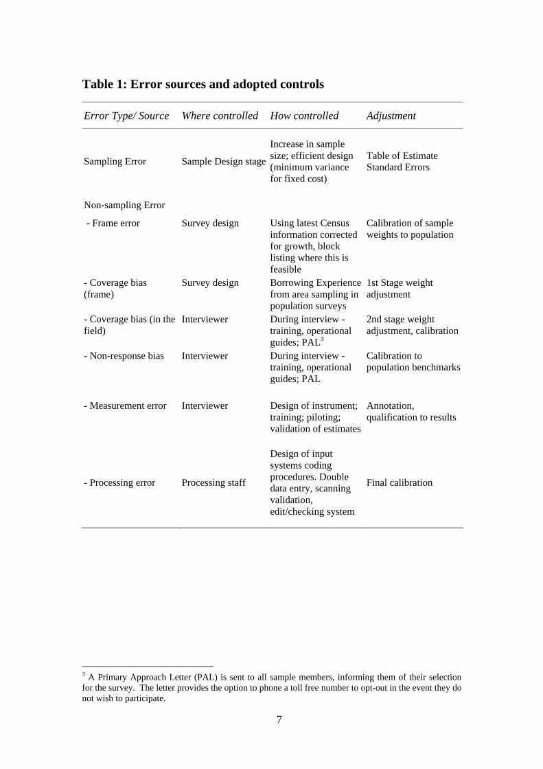
Table 1: Error sources and adopted controls

Error Type/ Source Where controlled How controlled Adjustment

Sampling Error Sample Design stage

Increase in sample size; efficient design (minimum variance for fixed cost)

Table of Estimate Standard Errors

Non-sampling Error

- Frame error Survey design Using latest Census information corrected for growth, block listing where this is feasible

Calibration of sample weights to population

- Coverage bias (frame)

Survey design Borrowing Experience from area sampling in population surveys

1st Stage weight adjustment

- Coverage bias (in the field)

Interviewer During interview - training, operational guides; PAL3

2nd stage weight adjustment, calibration

- Non-response bias Interviewer During interview - training, operational guides; PAL

Calibration to population benchmarks

- Measurement error Interviewer Design of instrument;

training; piloting; validation of estimates

Annotation, qualification to results

- Processing error Processing staff

Design of input systems coding procedures. Double data entry, scanning validation, edit/checking system

Final calibration

3 A Primary Approach Letter (PAL) is sent to all sample members, informing them of their selection for the survey. The letter provides the option to phone a toll free number to opt-out in the event they do not wish to participate.

7

Measuring Sampling Variability

Because the estimates derive from a sample rather than from the entire population, they will exhibit sampling error: that is a different draw would give a slightly different result. Sample error is a function of the sample size and sample design - how the sample was drawn. Where the sample is drawn at random it is conveniently measured using the estimate Standard Error, the standard deviation of the sample estimate viewed as one realisation out of many possible samples. This is calculated from sample values alone, and reflects both unequal sampling probabilities and population variability. The tables below list representative Relative Standard Errors (the Standard Error divided by the estimate) for different estimate levels for households and for responding and enumerated persons. The method employed to derive various functional forms for RSEs in the tables is explained in Attachment 1.

8

Standard Errors of Household Estimates

HILDA collects data on households and persons within households. The household estimates have been weighted using the SAS macro GREGWT. The method employs a multiphase generalised linear weight, incorporating information about differential probabilities of selection from the sample design, adjustment for non-response, and calibration to independent household benchmarks.

To estimate standard errors the weighting procedure is re-run against replicated datasets in which groups of records are systematically withdrawn. Variation between estimates from the replicates provides an estimator for the standard error of the weighted estimates from the full file. The choice of unit of replication should coincide with the primary clustering level – the PSU. By varying this unit, some insight into the effects of the clustering (and stratification) is possible. Further details about the theory of the jackknife method can be found in Wolter, and in pp 437-442 of Saerndal et al. The program used to weight the file and to calculate jackknife SEs of weighted estimates was developed by Phillip Bell for the ABS4.

While standard errors for an individual population statistic can be estimated using this technique, it is possible to exploit the expected relation between estimate size and relative standard error to derive representative Standard Errors that can serve as general guide for users of the data. The table below gives, not the jack-knife SEs themselves, but modelled values for the RSEs based on a curve fit to the scatter of a large number of plotted independent estimates and their jackknife RSEs. The tight fit to the curve gives some assurance that the definition of the table of estimates used to generate the pairs is not critical. The point of the table is not to exactly measure RSEs, but to guide the use of the underlying statistics, and in particular to highlight the limits imposed by sampling error on inference. This is illustrated in Examples1 & 2 below.

To refine the RSE measure for analysis, models are reported for the population as a whole and for certain subpopulations. That is, it is not unreasonable to expect the relation between estimates and RSEs to vary according to the population, depending on underlying variability within that population. Households in the smaller states (SA) for instance may be either more homogenous or more heterogenous compared to the larger states (NSW). The table separates out these anticipated effects. On the whole the influence of subpopulations on the functional fit is minor - for most purposes the left most (all State) column should suffice.

The tables incorporate suggested standard cut-offs; that is the threshold estimate levels below which high variability makes inference too uncertain for most use. Cut-offs of 50% and 25% have been used in line with ABS practice: estimates above the 25% cut-off point can be used without qualification; estimates with RSEs between 25 and 50% with the qualification that they are subject to high variability; and where RSE exceeds 50% should be suppressed or used only when the lack of reliability is understood. These levels and their use are conventional, and subject to assumptions used in modelling RSEs, and the context in which the statistics are quoted.

4 See The GREGWT and TABLE macros - Users Guide, ABS 2000 (uncatalogued) for more details

9

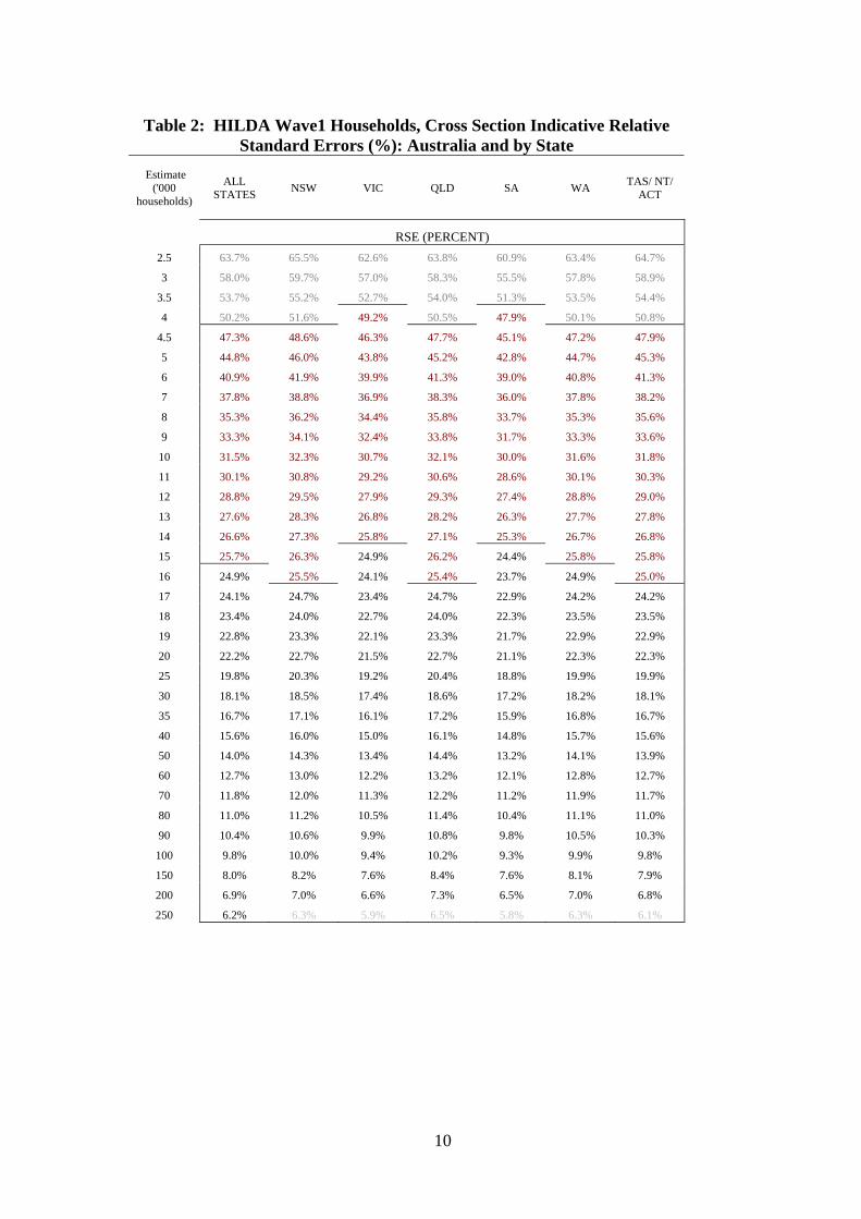
Table 2: HILDA Wave1 Households, Cross Section Indicative Relative Standard Errors (%): Australia and by State

Estimate ('000

households)

ALL STATES NSW VIC QLD SA WA TAS/ NT/

ACT

RSE (PERCENT) 2.5 63.7% 65.5% 62.6% 63.8% 60.9% 63.4% 64.7%

3 58.0% 59.7% 57.0% 58.3% 55.5% 57.8% 58.9%

3.5 53.7% 55.2% 52.7% 54.0% 51.3% 53.5% 54.4%

4 50.2% 51.6% 49.2% 50.5% 47.9% 50.1% 50.8%

4.5 47.3% 48.6% 46.3% 47.7% 45.1% 47.2% 47.9%

5 44.8% 46.0% 43.8% 45.2% 42.8% 44.7% 45.3%

6 40.9% 41.9% 39.9% 41.3% 39.0% 40.8% 41.3%

7 37.8% 38.8% 36.9% 38.3% 36.0% 37.8% 38.2%

8 35.3% 36.2% 34.4% 35.8% 33.7% 35.3% 35.6%

9 33.3% 34.1% 32.4% 33.8% 31.7% 33.3% 33.6%

10 31.5% 32.3% 30.7% 32.1% 30.0% 31.6% 31.8%

11 30.1% 30.8% 29.2% 30.6% 28.6% 30.1% 30.3%

12 28.8% 29.5% 27.9% 29.3% 27.4% 28.8% 29.0%

13 27.6% 28.3% 26.8% 28.2% 26.3% 27.7% 27.8%

14 26.6% 27.3% 25.8% 27.1% 25.3% 26.7% 26.8%

15 25.7% 26.3% 24.9% 26.2% 24.4% 25.8% 25.8%

16 24.9% 25.5% 24.1% 25.4% 23.7% 24.9% 25.0%

17 24.1% 24.7% 23.4% 24.7% 22.9% 24.2% 24.2%

18 23.4% 24.0% 22.7% 24.0% 22.3% 23.5% 23.5%

19 22.8% 23.3% 22.1% 23.3% 21.7% 22.9% 22.9%

20 22.2% 22.7% 21.5% 22.7% 21.1% 22.3% 22.3%

25 19.8% 20.3% 19.2% 20.4% 18.8% 19.9% 19.9%

30 18.1% 18.5% 17.4% 18.6% 17.2% 18.2% 18.1%

35 16.7% 17.1% 16.1% 17.2% 15.9% 16.8% 16.7%

40 15.6% 16.0% 15.0% 16.1% 14.8% 15.7% 15.6%

50 14.0% 14.3% 13.4% 14.4% 13.2% 14.1% 13.9%

60 12.7% 13.0% 12.2% 13.2% 12.1% 12.8% 12.7%

70 11.8% 12.0% 11.3% 12.2% 11.2% 11.9% 11.7%

80 11.0% 11.2% 10.5% 11.4% 10.4% 11.1% 11.0%

90 10.4% 10.6% 9.9% 10.8% 9.8% 10.5% 10.3%

100 9.8% 10.0% 9.4% 10.2% 9.3% 9.9% 9.8%

150 8.0% 8.2% 7.6% 8.4% 7.6% 8.1% 7.9%

200 6.9% 7.0% 6.6% 7.3% 6.5% 7.0% 6.8%

250 6.2% 6.3% 5.9% 6.5% 5.8% 6.3% 6.1%

10

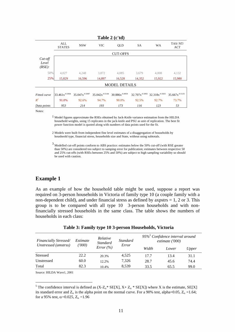
Table 2 (c'td)

ALL STATES NSW VIC QLD SA WA TAS/ NT/

ACT

CUT-OFFS Cut-off Level

(RSE): 50% 4,027 4,248 3,872 4,085 3,679 4,008 4,132

25% 15,829 16,596 14,897 16,528 14,352 15,922 15,980

MODEL DETAILS

Fitted curve 33.461x-0.5064 35.047x-0.5087 35.042x-0.5144 30.886x-0.4959 32.707x-0.5092 32.318x-0.5025 35.667x-0.5125

R2 91.0% 92.6% 94.7% 90.0% 92.5% 92.7% 73.7%

Data points 953 214 193 173 116 123 53

Notes: 1

Model figures approximate the RSEs obtained by Jack-Knife variance estimation from the HILDA household weights, using 15 replicates in the jack-knife and PSU as unit of replication. The best fit power function model is quoted along with numbers of data points used for the fit.

2

Models were built from independent fine level estimates of a disaggregation of households by housheold type, financial stress, households size and State, without using subtotals.

3

Modelled cut-off points conform to ABS practice: estimates below the 50% cut-off (with RSE greater than 50%) are considered too subject to samping error for publication; estimates between respective 50 and 25% cut-offs (with RSEs between 25% and 50%) are subject to high sampling variability so should be used with caution.

Example 1

As an example of how the household table might be used, suppose a report was required on 3-person households in Victoria of family type 10 (a couple family with a non-dependent child), and under financial stress as defined by axpstrs = 1, 2 or 3. This group is to be compared with all type 10 3-person households and with non-financially stressed households in the same class. The table shows the numbers of households in each class:

Table 3: Family type 10 3-person Households, Victoria

95%5 Confidence interval around estimate ('000) Financially Stressed/

Unstressed (amstrss)Estimate

('000)

Relative Standard Error (%)

Standard Error

Width Lower Upper

Stressed 22.2 20.3% 4,525 17.7 13.4 31.1 Unstressed 60.0 12.2% 7,326 28.7 45.6 74.4 Total 82.3 10.4% 8,539 33.5 65.5 99.0 Source: HILDA Wave1, 2001

5 The confidence interval is defined as (X-Zα* SE[X], X+ Zα * SE[X]) where X is the estimate, SE[X] its standard error and Zα is the alpha point on the normal curve. For a 90% test, alpha=0.05, Zα =1.64; for a 95% test, α=0.025, Zα =1.96

11

The RSEs for the stressed and total estimates have been interpolated from the respective tabulated figures. Thus the Victorian column of the table gives RSEs for 20,000 and 25,000 respectively as 21.5% and 19.2%. 22,200 represents 44% (2.2/5) of the way between these figures; 44% of the RSE difference (2.3%) is 1.01%, so the interpolated RSE for 22,200 is 21.5-1.0=20.5. Likewise 82,300 is 23% of the interval 80-90,000, so interpolated RSE for 82,300 is that for 80,000 (10.5 from the table) less 23% of the difference in RSEs for 80,000 and 90,000 (RSE=9.9%), namely 23% of .6%, or .2%, giving an interpolated RSE for 82,300 of 10.3%.

This table indicates that in 95% of cases (so with a high probability) the intervals (13.4, 31.1) (45.6, 74.4) and (65.5, 99), expressed as thousands of households, will contain the true values for respectively financially stressed, unstressed and total 3-person households of family type10 in Victoria. The corresponding intervals when RSEs are directly estimated rather than modelled are similar: (15.2,29.3), (43.8,76.2), (65.8,98.7): these however would be subject to extra variability implicit in the jack knife procedure. The modelled RSEs should serve as a more reliable a guide to how precise a statement we can make concerning the sizes of these classes of households, at least at the time of taking the survey.

Example 2

We may wish to go further and compare the financial stress of households from different types (or different states), and test for significant differences. Let us consider whether households with a nondependent child are less financially stressed than their counterparts with dependents. More concretely we hypothesise that household types 10 and 4 of size 3 in Victoria have the same degree of financial stress; and reject this hypothesis only if there is found a significant difference in the proportion of stressed households between the two classes.

Table 4: Type 4 Households of size 3*, Victoria 95% Confidence interval around

estimate ('000) Financially Stressed/ Unstressed (amstrss)

Estimate ('000)

Relative Standard Error (%)

Standard Error

Width Lower Upper

Stressed 41.7 14.7% 6,143 24.1 29.7 53.8 Unstressed 54.1 12.9% 6,966 27.3 40.4 67.7 Total 95.8 9.6% 9,196 36.0 77.8 113.9 Source: HILDA Wave1, 2001 *Defined as households constituted by a single family of Type4, comprising a couple and one dependent child To test the hypothesis we compare the stress prevalence rate (ratio of stressed households to total) between the two classes. The standard error on these rates is calculated using the following formula:

[ ] [ ] 22 )()( NRSEXRSENXRSE −=⎥⎦⎤

⎢⎣⎡

This formula applies when all elements of X belong to N.

12

The table below shows the result of applying the tabulated values for RSE to this formula.

Table 5: Financial Stress, 3-person Households, Victoria X N X/N RSE[X] RSE[N] RSE[X/N] Household Type 4 41.7 95.8 0.44 0.15 0.10 0.11

Household Type 10 22.2 82.3 0.27 0.20 0.10 0.17

Source: HILDA Wave1, 2001

The estimate of 44% of 3-person type4 households under financial stress compares with a rate of 27% for type10 households. Is the difference in rates significant?

To test this we require a further formula, in order to arrive at a standard error estimate for the difference in rates. This formula relates the variance (the square of the standard error) of the difference in rates to the respective rate variances:

⎥⎦

⎤⎢⎣

⎡+⎥

⎦

⎤⎢⎣

⎡=⎥

⎦

⎤⎢⎣

⎡−

2

2

1

1

2

2

1

1

NX

VarNX

VarNX

NX

Var

Noting that ( ) ( ){ } ( ){ } ( )222

nx

nxRSEn

xSEnxVar ×== we can set out the calculations

in a table.

Table 6: Test for significance in Financial Stress Rate difference Var (S1) 0.002361166 Var(S1-S2) 0.004599395 Var (S2) 0.002238229 SE (S1-S2) 0.06781884

S1-S2 0.17 Width (95%CI) 0.265849852 CI(Upper) 0.43 CI(Lower) -0.10 Notes: 1. S is the proportion of households under financial stress in the given population class as measured by axpstres

2. Var is the variance attached to the estimate, that is the square of its standard error (SE)

This shows the 95% confidence interval for the rate difference as including zero, so we are not justified in rejecting the original hypothesis in favour of an alternative that the rates differ (that is a two-tailed test). If the alternative had been that 3-person type4 households suffered more stress than type10 households (for instance if we had been investigating potential disadvantage associated with this household type), we would have rejected the hypothesis. In this case the width of the confidence interval halves, and the lower bound is positive.

From this we can conclude that the passage of the child in a couple plus child household in Victoria from dependent to nondependent status indeed lowers financial stress, in accord with expectations, but the association is not very strong. This qualification belies the dramatic drop in financial stress index in moving from family

13

type4 to 10 amongst these households, reflecting the relatively small size of underlying populations of households.

Standard Errors of Responding Person Estimates

The survey collected information in stages. In the first instance it collected details of the household selected in sample – its composition and characteristics at this level, such as tenure, size and housing costs and use of child care within the household. These were recorded on a household form. Standard Errors for estimates from this part of the survey can be calculated using table 2. In the second stage information was sought from each adult (persons aged 15 years and over) resident in the household. All completed schedules from persons responding at this level comprise the responding persons file. Estimates derived from this file, using information collected from personal interviews, are also subject to sampling error.

Table 7 gives indicative RSEs (%) for estimates using the responding persons file, for all persons, and for females and males separately; and for the different marital status classes. The slight variation in cut-offs between classes indicates that a general model suffices for most purposes, that is the all-person figures approximate reasonably well the subgroups. Where confidence bounds are critical it may be advisable to use the model appropriate to the particular subpopulation.

14

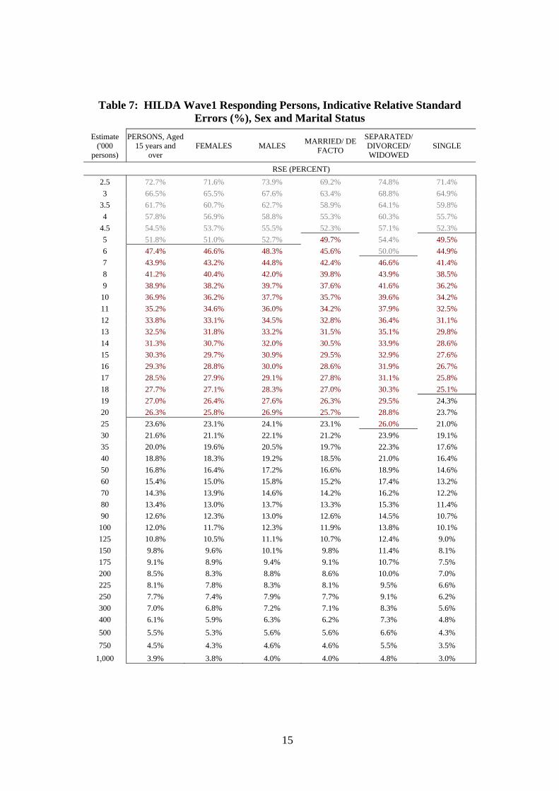
Table 7: HILDA Wave1 Responding Persons, Indicative Relative Standard Errors (%), Sex and Marital Status

Estimate ('000

persons)

PERSONS, Aged 15 years and

over FEMALES MALES MARRIED/ DE

FACTO

SEPARATED/ DIVORCED/ WIDOWED

SINGLE

RSE (PERCENT) 2.5 72.7% 71.6% 73.9% 69.2% 74.8% 71.4% 3 66.5% 65.5% 67.6% 63.4% 68.8% 64.9%

3.5 61.7% 60.7% 62.7% 58.9% 64.1% 59.8% 4 57.8% 56.9% 58.8% 55.3% 60.3% 55.7%

4.5 54.5% 53.7% 55.5% 52.3% 57.1% 52.3% 5 51.8% 51.0% 52.7% 49.7% 54.4% 49.5% 6 47.4% 46.6% 48.3% 45.6% 50.0% 44.9% 7 43.9% 43.2% 44.8% 42.4% 46.6% 41.4% 8 41.2% 40.4% 42.0% 39.8% 43.9% 38.5% 9 38.9% 38.2% 39.7% 37.6% 41.6% 36.2%

10 36.9% 36.2% 37.7% 35.7% 39.6% 34.2% 11 35.2% 34.6% 36.0% 34.2% 37.9% 32.5% 12 33.8% 33.1% 34.5% 32.8% 36.4% 31.1% 13 32.5% 31.8% 33.2% 31.5% 35.1% 29.8% 14 31.3% 30.7% 32.0% 30.5% 33.9% 28.6% 15 30.3% 29.7% 30.9% 29.5% 32.9% 27.6% 16 29.3% 28.8% 30.0% 28.6% 31.9% 26.7% 17 28.5% 27.9% 29.1% 27.8% 31.1% 25.8% 18 27.7% 27.1% 28.3% 27.0% 30.3% 25.1% 19 27.0% 26.4% 27.6% 26.3% 29.5% 24.3% 20 26.3% 25.8% 26.9% 25.7% 28.8% 23.7% 25 23.6% 23.1% 24.1% 23.1% 26.0% 21.0% 30 21.6% 21.1% 22.1% 21.2% 23.9% 19.1% 35 20.0% 19.6% 20.5% 19.7% 22.3% 17.6% 40 18.8% 18.3% 19.2% 18.5% 21.0% 16.4% 50 16.8% 16.4% 17.2% 16.6% 18.9% 14.6% 60 15.4% 15.0% 15.8% 15.2% 17.4% 13.2% 70 14.3% 13.9% 14.6% 14.2% 16.2% 12.2% 80 13.4% 13.0% 13.7% 13.3% 15.3% 11.4% 90 12.6% 12.3% 13.0% 12.6% 14.5% 10.7% 100 12.0% 11.7% 12.3% 11.9% 13.8% 10.1% 125 10.8% 10.5% 11.1% 10.7% 12.4% 9.0% 150 9.8% 9.6% 10.1% 9.8% 11.4% 8.1% 175 9.1% 8.9% 9.4% 9.1% 10.7% 7.5% 200 8.5% 8.3% 8.8% 8.6% 10.0% 7.0% 225 8.1% 7.8% 8.3% 8.1% 9.5% 6.6% 250 7.7% 7.4% 7.9% 7.7% 9.1% 6.2% 300 7.0% 6.8% 7.2% 7.1% 8.3% 5.6% 400 6.1% 5.9% 6.3% 6.2% 7.3% 4.8% 500 5.5% 5.3% 5.6% 5.6% 6.6% 4.3% 750 4.5% 4.3% 4.6% 4.6% 5.5% 3.5%

1,000 3.9% 3.8% 4.0% 4.0% 4.8% 3.0%

15

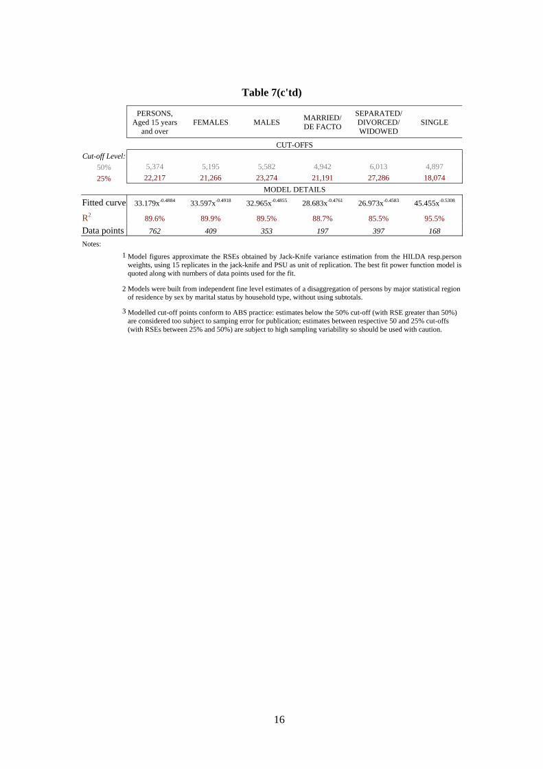
Table 7(c'td)

PERSONS,

Aged 15 years and over

FEMALES MALES MARRIED/ DE FACTO

SEPARATED/ DIVORCED/ WIDOWED

SINGLE

CUT-OFFS Cut-off Level:

50% 5,374 5,195 5,582 4,942 6,013 4,897 25% 22,217 21,266 23,274 21,191 27,286 18,074

MODEL DETAILS

Fitted curve 33.179x-0.4884 33.597x-0.4918 32.965x-0.4855 28.683x-0.4761 26.973x-0.4583 45.455x-0.5308

R2 89.6% 89.9% 89.5% 88.7% 85.5% 95.5% Data points 762 409 353 197 397 168 Notes:

1

Model figures approximate the RSEs obtained by Jack-Knife variance estimation from the HILDA resp.person weights, using 15 replicates in the jack-knife and PSU as unit of replication. The best fit power function model is quoted along with numbers of data points used for the fit.

2

Models were built from independent fine level estimates of a disaggregation of persons by major statistical region of residence by sex by marital status by household type, without using subtotals.

3

Modelled cut-off points conform to ABS practice: estimates below the 50% cut-off (with RSE greater than 50%) are considered too subject to samping error for publication; estimates between respective 50 and 25% cut-offs (with RSEs between 25% and 50%) are subject to high sampling variability so should be used with caution.

16

Standard Errors of Enumerated Persons Estimates

The HILDA Wave1 Enumerated persons file comprises records of all persons listed as residing in houses for which a completed household form is available. Unlike the responding persons case the enumerated persons file includes records of children (under 15 years of age, who are not interviewed so do not contribute person questionnaires), and usual residents in selected and responding households who did not respond to the survey. This file thus contains a more complete sample of the underlying household population, and can be expected to give more accurate person estimates over the restricted set of household level variables for which information is available.

Table 8 shows modeled relative standard errors against estimate levels for estimates from the enumerated persons file, for all persons, and for persons in various household types, with type based on numbers of adults and numbers of children living in them.

17

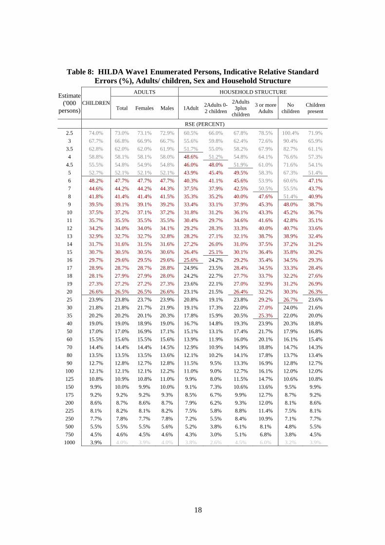
Table 8: HILDA Wave1 Enumerated Persons, Indicative Relative Standard Errors (%), Adults/ children, Sex and Household Structure

ADULTS HOUSEHOLD STRUCTURE Estimate ('000

persons) CHILDREN

Total Females Males 1Adult 2Adults 0-2 children

2Adults 3plus

children

3 or more Adults

No children

Children present

RSE (PERCENT) 2.5 74.0% 73.0% 73.1% 72.9% 60.5% 66.0% 67.8% 78.5% 100.4% 71.9% 3 67.7% 66.8% 66.9% 66.7% 55.6% 59.8% 62.4% 72.6% 90.4% 65.9%

3.5 62.8% 62.0% 62.0% 61.9% 51.7% 55.0% 58.2% 67.9% 82.7% 61.1% 4 58.8% 58.1% 58.1% 58.0% 48.6% 51.2% 54.8% 64.1% 76.6% 57.3%

4.5 55.5% 54.8% 54.9% 54.8% 46.0% 48.0% 51.9% 61.0% 71.6% 54.1% 5 52.7% 52.1% 52.1% 52.1% 43.9% 45.4% 49.5% 58.3% 67.3% 51.4% 6 48.2% 47.7% 47.7% 47.7% 40.3% 41.1% 45.6% 53.9% 60.6% 47.1% 7 44.6% 44.2% 44.2% 44.3% 37.5% 37.9% 42.5% 50.5% 55.5% 43.7% 8 41.8% 41.4% 41.4% 41.5% 35.3% 35.2% 40.0% 47.6% 51.4% 40.9% 9 39.5% 39.1% 39.1% 39.2% 33.4% 33.1% 37.9% 45.3% 48.0% 38.7%

10 37.5% 37.2% 37.1% 37.2% 31.8% 31.2% 36.1% 43.3% 45.2% 36.7% 11 35.7% 35.5% 35.5% 35.5% 30.4% 29.7% 34.6% 41.6% 42.8% 35.1% 12 34.2% 34.0% 34.0% 34.1% 29.2% 28.3% 33.3% 40.0% 40.7% 33.6% 13 32.9% 32.7% 32.7% 32.8% 28.2% 27.1% 32.1% 38.7% 38.9% 32.4% 14 31.7% 31.6% 31.5% 31.6% 27.2% 26.0% 31.0% 37.5% 37.2% 31.2% 15 30.7% 30.5% 30.5% 30.6% 26.4% 25.1% 30.1% 36.4% 35.8% 30.2% 16 29.7% 29.6% 29.5% 29.6% 25.6% 24.2% 29.2% 35.4% 34.5% 29.3% 17 28.9% 28.7% 28.7% 28.8% 24.9% 23.5% 28.4% 34.5% 33.3% 28.4% 18 28.1% 27.9% 27.9% 28.0% 24.2% 22.7% 27.7% 33.7% 32.2% 27.6% 19 27.3% 27.2% 27.2% 27.3% 23.6% 22.1% 27.0% 32.9% 31.2% 26.9% 20 26.6% 26.5% 26.5% 26.6% 23.1% 21.5% 26.4% 32.2% 30.3% 26.3% 25 23.9% 23.8% 23.7% 23.9% 20.8% 19.1% 23.8% 29.2% 26.7% 23.6% 30 21.8% 21.8% 21.7% 21.9% 19.1% 17.3% 22.0% 27.0% 24.0% 21.6% 35 20.2% 20.2% 20.1% 20.3% 17.8% 15.9% 20.5% 25.3% 22.0% 20.0% 40 19.0% 19.0% 18.9% 19.0% 16.7% 14.8% 19.3% 23.9% 20.3% 18.8% 50 17.0% 17.0% 16.9% 17.1% 15.1% 13.1% 17.4% 21.7% 17.9% 16.8% 60 15.5% 15.6% 15.5% 15.6% 13.9% 11.9% 16.0% 20.1% 16.1% 15.4% 70 14.4% 14.4% 14.4% 14.5% 12.9% 10.9% 14.9% 18.8% 14.7% 14.3% 80 13.5% 13.5% 13.5% 13.6% 12.1% 10.2% 14.1% 17.8% 13.7% 13.4% 90 12.7% 12.8% 12.7% 12.8% 11.5% 9.5% 13.3% 16.9% 12.8% 12.7% 100 12.1% 12.1% 12.1% 12.2% 11.0% 9.0% 12.7% 16.1% 12.0% 12.0% 125 10.8% 10.9% 10.8% 11.0% 9.9% 8.0% 11.5% 14.7% 10.6% 10.8% 150 9.9% 10.0% 9.9% 10.0% 9.1% 7.3% 10.6% 13.6% 9.5% 9.9% 175 9.2% 9.2% 9.2% 9.3% 8.5% 6.7% 9.9% 12.7% 8.7% 9.2% 200 8.6% 8.7% 8.6% 8.7% 7.9% 6.2% 9.3% 12.0% 8.1% 8.6% 225 8.1% 8.2% 8.1% 8.2% 7.5% 5.8% 8.8% 11.4% 7.5% 8.1% 250 7.7% 7.8% 7.7% 7.8% 7.2% 5.5% 8.4% 10.9% 7.1% 7.7% 500 5.5% 5.5% 5.5% 5.6% 5.2% 3.8% 6.1% 8.1% 4.8% 5.5% 750 4.5% 4.6% 4.5% 4.6% 4.3% 3.0% 5.1% 6.8% 3.8% 4.5%

1000 3.9% 4.0% 3.9% 4.0% 3.8% 2.6% 4.5% 6.0% 3.2% 3.9%

18

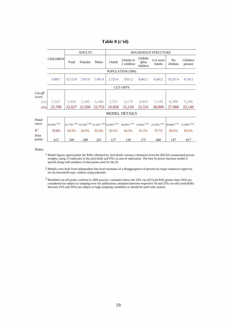
Table 8 (c'td)

ADULTS HOUSEHOLD STRUCTURE

CHILDREN Total Females Males 1Adult 2Adults 0-

2 children

2Adults 3plus

children

3 or more Adults

No children

Children present

POPULATION ('000)

3,889.7 15,123.9 7,631.9 7,491.9 2,725.4 3,811.2 8,462.1 6,045.2 10,257.4 8,756.2

CUT-OFFS

Cut-off Level:

50% 5,557 5,440 5,440 5,440 3,767 4,179 4,893 7,149 8,388 5,296 25% 22,768 22,627 22,500 22,753 16,828 15,110 22,531 36,000 27,968 22,146

MODEL DETAILS Fitted curve 34.639x-0.4915 32.779x-0.4863 33.318x-0.4882 32.247x-0.4844 22.647x-0.4631 44.855x-0.5393 23.641x-0.4539 22.474x-0.4288 90.664x-0.5756 31.859x-0.4845

R2 78.8% 84.9% 84.9% 85.0% 82.0% 84.9% 81.5% 79.7% 89.0% 80.0% Data points 415 549 288 261 127 130 175 468 147 817

Notes: 1

Model figures approximate the RSEs obtained by Jack-Knife variance estimation from the HILDA enumerated person weights, using 15 replicates in the jack-knife and PSU as unit of replication. The best fit power function model is quoted along with numbers of data points used for the fit.

2

Models were built from independent fine level estimates of a disaggregation of persons by major statistical region by sex by household type, without using subtotals.

3

Modelled cut-off points conform to ABS practice: estimates below the 50% cut-off (with RSE greater than 50%) are considered too subject to samping error for publication; estimates between respective 50 and 25% cut-offs (with RSEs between 25% and 50%) are subject to high sampling variability so should be used with caution.

19

Standard Errors for Complex statistics

The tables above can be used to give confidence intervals for simple estimates of households and persons from the HILDA Survey, and for tests of hypothesis concerning proportions. Typical applications of the survey data result in estimates of model parameters. These being based on sample estimates, rather than data drawn from knowledge of the population as a whole, have a sample error component on top of the error terms incorporated in the models. It is therefore of some interest to derive standard errors and confidence intervals for such parameters. The replicate weights can be used for this purpose; although the straightforward curve fit models used to give indicative RSEs for simple estimates will not apply. The calculation of standard errors for regression parameters is discussed by Kish and Frankel, and can be implemented using the jack-knife program built into the TABLE macro component of GREGWEIGHT.

Standard Errors for flows

The primary purpose of HILDA is to measure changes in individual circumstances and how past may interact with current circumstance. It does this by tracking a sampled panel over time. Sample error attaches to cross section estimates at each wave of the survey; it also attaches to estimates of flow between waves. It is important to account for the standard error in any analysis involving flow estimates. How to arrive at a realistic estimate of flow standard errors is not immediately clear. A conservative approach is to compound the standard errors from the respective cross sections. This however should be an overestimate of error given the large measure of correlation between the two estimates. A realistic standard error approach then hinges on estimates of inter-wave correlation in point in time estimates.

The standard error of a flow statistic such as “People in class A at time t; who had left A by time t+1” is approximated by the error attached to the estimate of gross flow as measured at one or the other time point defining the flow. More precisely, this error can be estimated using the accumulating weighted wave file. This will take account of the reduction in sample between the waves, and the inflation in weights and weight variability.

It should be noted an estimate of flow is not a simple class estimate. It incorporates an implicit propensity to leave (or enter) a state, attached to an individual; standard error for the propensity might be better modelled using survival curves, which themselves are qualified by sampling error in their parameters. A more complete account of flow standard error will accompany releases of multiple wave data when candidate wave weights will be available.

Treatment of standard errors in panel data for comparable surveys is outlined in Attachment 1 (an extract from a 2001 HILDA Discussion paper by Henstridge).

20

References

Stuart, B. (1964) Basic Ideas of Scientific Sampling, Charles Griffin & Co., London

Wolter, K. M. (1985) Introduction to Variance Estimation, Springer Verlag, New York

Saerndal, C.-E., Swensson, B., Wretman, J. (1992) Model Assisted Survey Sampling, Springer Verlag, New York

Kish, L. and M. Frankel (1974) ‘Inference from Complex Statistics’, originally published in Journal of the Royal Statistical Society 36, Ser. B, 1-22, and republished as chapter 8 in Leslie Kish, Selected papers (eds. Kalton, G.. and Heeringa, S.), John Wiley and Sons, Hoboken 2002

.

21

Attachment 1

Estimation of standard errors for panel data

[extracted from John Henstridge, The Household Income and Labour Dynamics in Australia (HILDA) Survey: Weighting and Imputation, HILDA Project Discussion Paper Series, No. 3/01, July 2001]

The following rules will mean that after Wave 1 some households in the sample will be related to each other, having derived from the same Wave 1 household. In addition, there will be a structure related to having several individuals in each household. These will give a complex correlation structure on the data in addition to the normal effects due to the cluster design.

The only feasible methods of calculating such standard errors collectively termed resampling procedures, and include the jackknife, bootstrapping and ‘half sample’ methods. (See for example Lehtonen and Pahkinen, 1992.)

For example, Rendtel (1991) applied a ‘random groups’ procedure to the GSOEP data to investigate the development of sampling errors over waves. With each wave, the panel will have a sample of households, each of which can be linked back to one household in Wave 1. Since households can and will drop out but none can enter except via a link to the Wave 1 sample, the number of Wave 1 households remaining relevant to the current panel can only diminish. This will lead to an increase in the correlation between panel households and a subsequent increase in standard errors. The level of this increase will depend upon the item being considered, being the greatest for items that might be ‘inherited’. The example given by Rendtel suggests that over five years the standard error for estimates of political preference increased by 14% due to this effect alone, corresponding to a drop in sample efficiency of 24%.

These increases in standard errors can be reduced by minimising attrition. The only way to avoid the effect is through the addition of new households not related to the original ones.

References

Rendtel, U. (1991) ‘Weighting procedures and sampling variance in household panels’, Working Papers of the European Science Foundation Scientific Network on Household Panel Studies, No. 11, Essex.

Lehtonen, R. and Pahkinen, E. J. (1994) Practical Methods for Design and Analysis of Complex Surveys, revised Edition, John Wiley and Sons, Chichester.

22

Attachment 2

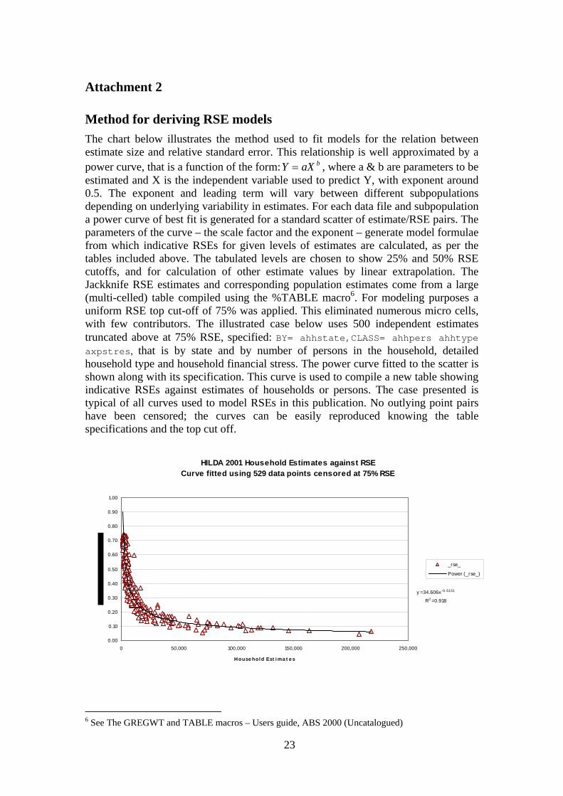
Method for deriving RSE models The chart below illustrates the method used to fit models for the relation between estimate size and relative standard error. This relationship is well approximated by a power curve, that is a function of the form: , where a & b are parameters to be estimated and X is the independent variable used to predict Y, with exponent around 0.5. The exponent and leading term will vary between different subpopulations depending on underlying variability in estimates. For each data file and subpopulation a power curve of best fit is generated for a standard scatter of estimate/RSE pairs. The parameters of the curve – the scale factor and the exponent – generate model formulae from which indicative RSEs for given levels of estimates are calculated, as per the tables included above. The tabulated levels are chosen to show 25% and 50% RSE cutoffs, and for calculation of other estimate values by linear extrapolation. The Jackknife RSE estimates and corresponding population estimates come from a large (multi-celled) table compiled using the %TABLE macro

baXY =

6. For modeling purposes a uniform RSE top cut-off of 75% was applied. This eliminated numerous micro cells, with few contributors. The illustrated case below uses 500 independent estimates truncated above at 75% RSE, specified: BY= ahhstate,CLASS= ahhpers ahhtype axpstres, that is by state and by number of persons in the household, detailed household type and household financial stress. The power curve fitted to the scatter is shown along with its specification. This curve is used to compile a new table showing indicative RSEs against estimates of households or persons. The case presented is typical of all curves used to model RSEs in this publication. No outlying point pairs have been censored; the curves can be easily reproduced knowing the table specifications and the top cut off.

HILDA 2001 Household Estimates against RSECurve fitted using 529 data points censored at 75% RSE

y = 34.606x-0.5151

R2 = 0.918

0.00

0.10

0.20

0.30

0.40

0.50

0.60

0.70

0.80

0.90

1.00

0 50,000 100,000 150,000 200,000 250,000

House hol d Est i ma t e s

_rse_

Power (_rse_)

6 See The GREGWT and TABLE macros – Users guide, ABS 2000 (Uncatalogued)

23

Attachment 3

Enumerated and Responding Person Estimate Variability Charted below are scatters of Estimate/RSE points for paired estimates from enumerated person and the responding person files. This shows a slight reduction in variability for the enumerated file, and no gross deviation between the estimates. The files differ by exclusion from the Responding person file (the main HILDA data set) of adult persons in responding households in scope for the survey but out on coverage or not responding, and in the calculation of weights. The enumerated file weights do not have access to labour force status, which has been used as one of the benchmark series for the responding weights. The discrepancy between the two series gives a measure of the bias from nonresponse, and the reduction in efficiency as a result of dropping nonresponding person records. This effect, barely detectable at a modeled level, is mitigated by the clustering within households7.

Comparison between Relative Standard Errors for paired Enumerated and Responding Persons estimates, HILDA Wave1

Responding Filey = 47.87x-0.5162

R2 = 0.8633

Enumerated filey = 45.489x-0.5144

R2 = 0.8578

0

1

0 50,000 100,000 150,000 200,000 250,000 300,000 350,000 400,000 450,000

Estimates

Rel

ativ

e St

anda

rd E

rror

_rse_resp

_rse_enum

Power (_rse_resp)

Power (_rse_enum)

7 The reduction in sample error from including all members in responding households, and not just responding members is discounted by the clustering of the new sample. Person non-response reduces this clustering.

24

HILDA 2001 Wave1, File Comparison - Enumerated and Responding Persons

Adults Females Males Metro ExMetro Estimate ('000

persons) Responding persons

Enumerated persons

Responding persons

Enumerated persons

Responding persons

Enumerated persons

Responding persons

Enumerated persons

Responding persons

Enumerated persons

INDICATIVE RELATIVE STANDARD ERRORS, ENUMERATED AND RESPONDING PERSON ESTIMATES

2.5 84.3% 81.3% 84.4% 80.3% 84.3% 82.5% 89.7% 85.7% 82.8% 80.9%

3 76.8% 74.0% 76.8% 73.2% 76.8% 75.1% 81.6% 78.1% 75.3% 73.4%

3.5 70.9% 68.4% 70.8% 67.6% 71.0% 69.3% 75.4% 72.2% 69.4% 67.7%

4 66.2% 63.8% 66.1% 63.1% 66.3% 64.7% 70.3% 67.4% 64.7% 63.1%

4.5 62.3% 60.1% 62.2% 59.4% 62.4% 60.9% 66.2% 63.5% 60.8% 59.3%

5 59.0% 56.9% 58.8% 56.3% 59.1% 57.7% 62.7% 60.1% 57.5% 56.1%

6 53.7% 51.8% 53.5% 51.3% 53.9% 52.5% 57.1% 54.8% 52.2% 50.9%

7 49.6% 47.9% 49.4% 47.4% 49.8% 48.5% 52.7% 50.6% 48.2% 46.9%

8 46.3% 44.7% 46.1% 44.2% 46.5% 45.2% 49.2% 47.3% 44.9% 43.7%

9 43.5% 42.1% 43.3% 41.6% 43.8% 42.6% 46.3% 44.5% 42.2% 41.1%

10 41.2% 39.8% 41.0% 39.5% 41.5% 40.3% 43.8% 42.2% 39.9% 38.9%

11 39.3% 37.9% 39.0% 37.6% 39.5% 38.4% 41.7% 40.2% 38.0% 37.0%

12 37.5% 36.3% 37.3% 35.9% 37.8% 36.7% 39.9% 38.4% 36.3% 35.3%

13 36.0% 34.8% 35.8% 34.5% 36.3% 35.2% 38.3% 36.9% 34.8% 33.8%

14 34.7% 33.5% 34.4% 33.2% 34.9% 33.9% 36.8% 35.5% 33.4% 32.5%

15 33.4% 32.3% 33.2% 32.0% 33.7% 32.7% 35.5% 34.3% 32.2% 31.4%

16 32.4% 31.3% 32.1% 31.0% 32.6% 31.6% 34.4% 33.2% 31.2% 30.3%

17 31.4% 30.3% 31.1% 30.1% 31.6% 30.6% 33.3% 32.1% 30.2% 29.4%

18 30.4% 29.4% 30.2% 29.2% 30.7% 29.8% 32.4% 31.2% 29.3% 28.5%

19 29.6% 28.6% 29.4% 28.4% 29.8% 28.9% 31.5% 30.4% 28.5% 27.7%

20 28.8% 27.9% 28.6% 27.7% 29.1% 28.2% 30.6% 29.6% 27.7% 27.0%

22.5 27.1% 26.3% 26.9% 26.0% 27.4% 26.5% 28.8% 27.8% 26.0% 25.3%

25 25.7% 24.9% 25.5% 24.7% 25.9% 25.1% 27.3% 26.4% 24.6% 24.0%

30 23.4% 22.6% 23.2% 22.5% 23.6% 22.9% 24.9% 24.0% 22.4% 21.8%

35 21.6% 20.9% 21.4% 20.8% 21.8% 21.1% 22.9% 22.2% 20.6% 20.1%

40 20.2% 19.5% 19.9% 19.4% 20.4% 19.7% 21.4% 20.7% 19.2% 18.7%

45 19.0% 18.4% 18.8% 18.2% 19.2% 18.5% 20.2% 19.5% 18.1% 17.6%

50 18.0% 17.4% 17.8% 17.3% 18.2% 17.6% 19.1% 18.5% 17.1% 16.6%

55 17.1% 16.6% 16.9% 16.5% 17.3% 16.7% 18.2% 17.6% 16.3% 15.8%

60 16.4% 15.8% 16.2% 15.7% 16.6% 16.0% 17.4% 16.9% 15.5% 15.1%

65 15.7% 15.2% 15.5% 15.1% 15.9% 15.3% 16.7% 16.2% 14.9% 14.5%

70 15.1% 14.6% 14.9% 14.5% 15.3% 14.8% 16.0% 15.6% 14.3% 13.9%

75 14.6% 14.1% 14.4% 14.0% 14.8% 14.2% 15.5% 15.0% 13.8% 13.4%

80 14.1% 13.7% 13.9% 13.6% 14.3% 13.8% 15.0% 14.6% 13.3% 13.0%

85 13.7% 13.2% 13.5% 13.2% 13.9% 13.3% 14.5% 14.1% 12.9% 12.6%

90 13.3% 12.9% 13.1% 12.8% 13.5% 13.0% 14.1% 13.7% 12.5% 12.2%

95 12.9% 12.5% 12.7% 12.4% 13.1% 12.6% 13.7% 13.3% 12.2% 11.8%

100 12.6% 12.2% 12.4% 12.1% 12.8% 12.3% 13.3% 13.0% 11.9% 11.5%

125 11.2% 10.9% 11.0% 10.8% 11.4% 10.9% 11.9% 11.6% 10.5% 10.2%

150 10.2% 9.9% 10.0% 9.8% 10.4% 10.0% 10.8% 10.5% 9.6% 9.3%

175 9.4% 9.1% 9.3% 9.1% 9.6% 9.2% 10.0% 9.7% 8.8% 8.6%

200 8.8% 8.5% 8.6% 8.5% 8.9% 8.6% 9.3% 9.1% 8.2% 8.0%

300 7.1% 6.9% 7.0% 6.9% 7.3% 7.0% 7.6% 7.4% 6.7% 6.4%

400 6.1% 6.0% 6.0% 6.0% 6.3% 6.0% 6.5% 6.4% 5.7% 5.5%

500 5.5% 5.3% 5.4% 5.3% 5.6% 5.3% 5.8% 5.7% 5.1% 4.9%

750 4.4% 4.3% 4.3% 4.3% 4.5% 4.3% 4.7% 4.6% 4.1% 4.0%

1000 3.8% 3.7% 3.7% 3.7% 3.9% 3.7% 4.1% 4.0% 3.5% 3.4%

25

Popn ('000) 14,810.8 14,836.5 7,490.6 7,490.6 7,320.2 7,345.9 9,213.8 9,222.1 4,947.4 4,966.9

Sample counts 306 311 159 157 147 154 151 152 118 123

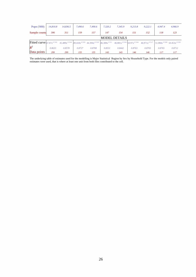
MODEL DETAILS Fitted curve 47.87x-0.5162 45.489x-0.5144 49.418x-0.5202 44.394x-0.5128 46.308x-0.512 46.881x-0.5164 50.97x-0.5164 46.971x-0.5117 51.084x-0.5268 50.453x-0.5283

R20.8633 0.8578 0.8727 0.8708 0.8531 0.8442 0.8763 0.8703 0.8765 0.8712

Data points 299 299 155 155 143 143 146 146 117 117

The underlying table of estimates used for the modelling is Major Statistical Region by Sex by Household Type. For the models only paired estimates were used, that is where at least one unit from both files contributed to the cell.

26

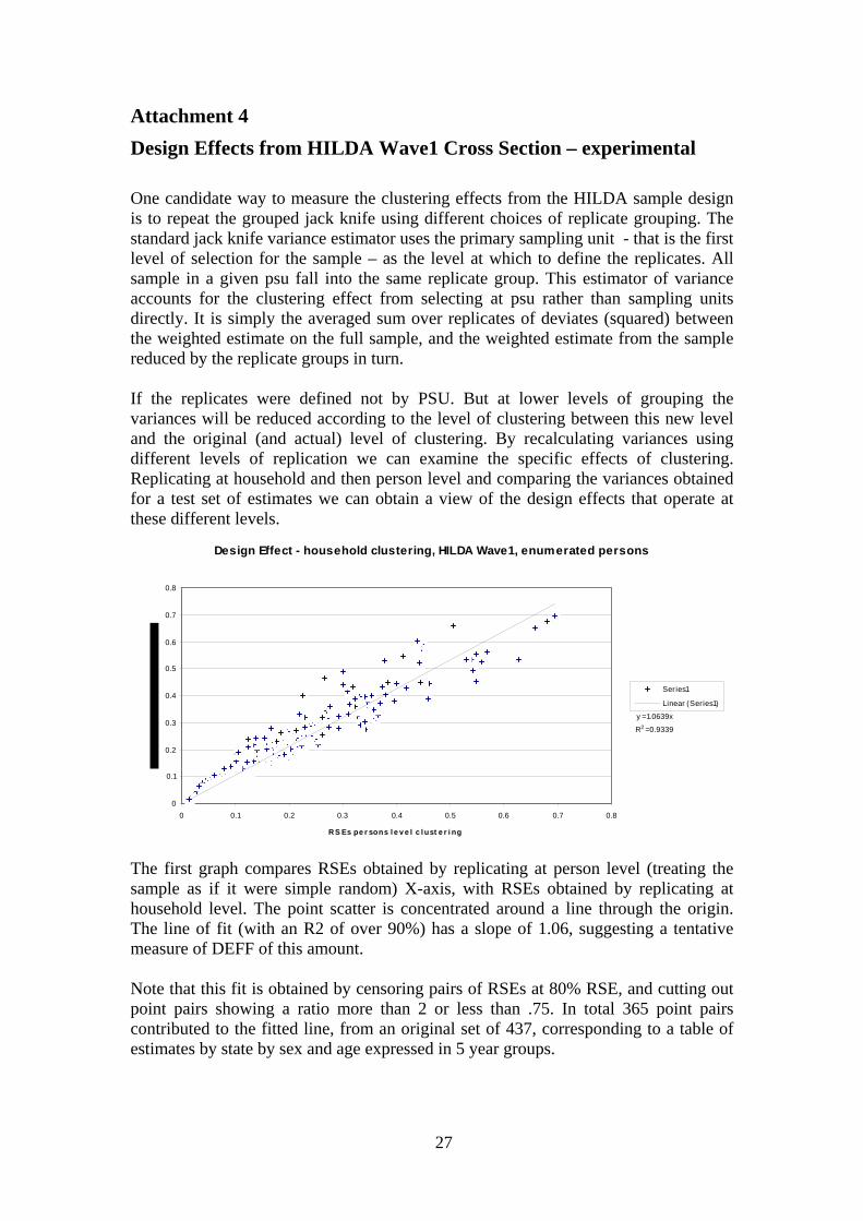
Attachment 4 Design Effects from HILDA Wave1 Cross Section – experimental One candidate way to measure the clustering effects from the HILDA sample design is to repeat the grouped jack knife using different choices of replicate grouping. The standard jack knife variance estimator uses the primary sampling unit - that is the first level of selection for the sample – as the level at which to define the replicates. All sample in a given psu fall into the same replicate group. This estimator of variance accounts for the clustering effect from selecting at psu rather than sampling units directly. It is simply the averaged sum over replicates of deviates (squared) between the weighted estimate on the full sample, and the weighted estimate from the sample reduced by the replicate groups in turn. If the replicates were defined not by PSU. But at lower levels of grouping the variances will be reduced according to the level of clustering between this new level and the original (and actual) level of clustering. By recalculating variances using different levels of replication we can examine the specific effects of clustering. Replicating at household and then person level and comparing the variances obtained for a test set of estimates we can obtain a view of the design effects that operate at these different levels.

Design Effect - household clustering, HILDA Wave1, enumerated persons

y = 1.0639x

R2 = 0.9339

0

0.1

0.2

0.3

0.4

0.5

0.6

0.7

0.8

0 0.1 0.2 0.3 0.4 0.5 0.6 0.7 0.8

RS Es pe r sons l e v e l c l ust e r i ng

Series1

Linear (Series1)

The first graph compares RSEs obtained by replicating at person level (treating the sample as if it were simple random) X-axis, with RSEs obtained by replicating at household level. The point scatter is concentrated around a line through the origin. The line of fit (with an R2 of over 90%) has a slope of 1.06, suggesting a tentative measure of DEFF of this amount. Note that this fit is obtained by censoring pairs of RSEs at 80% RSE, and cutting out point pairs showing a ratio more than 2 or less than .75. In total 365 point pairs contributed to the fitted line, from an original set of 437, corresponding to a table of estimates by state by sex and age expressed in 5 year groups.

27

Design Effect - psu clustering, HILDA Wave1, enumerated persons

y = 1.2236x

R2 = 0.8878

0

0.1

0.2

0.3

0.4

0.5

0.6

0.7

0.8

0.9

0 0.1 0.2 0.3 0.4 0.5 0.6 0.7 0.8

RS Es pe r sons l e v e l c l ust e r i ng

Series1

Linear (Series1)

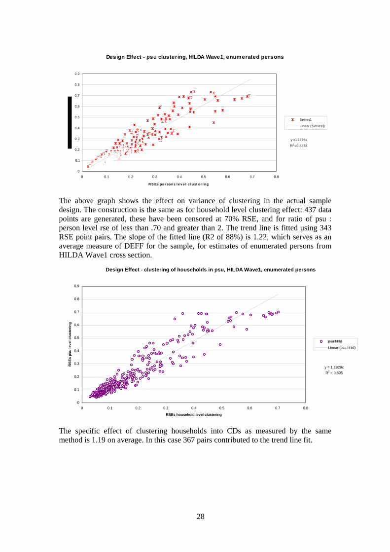
The above graph shows the effect on variance of clustering in the actual sample design. The construction is the same as for household level clustering effect: 437 data points are generated, these have been censored at 70% RSE, and for ratio of psu : person level rse of less than .70 and greater than 2. The trend line is fitted using 343 RSE point pairs. The slope of the fitted line (R2 of 88%) is 1.22, which serves as an average measure of DEFF for the sample, for estimates of enumerated persons from HILDA Wave1 cross section.

Design Effect - clustering of households in psu, HILDA Wave1, enumerated persons

y = 1.1929xR2 = 0.895

0

0.1

0.2

0.3

0.4

0.5

0.6

0.7

0.8

0.9

0 0.1 0.2 0.3 0.4 0.5 0.6 0.7 0.8

RSEs household level clustering

RSE

s ps

u le

vel c

lust

erin

g

psu:hhld

Linear (psu:hhld)

The specific effect of clustering households into CDs as measured by the same method is 1.19 on average. In this case 367 pairs contributed to the trend line fit.

28