motion estimation i - mit - massachusetts institute of technology
TRANSCRIPT


Last time
• Motion perception
• Motion representation
• Parametric motion: Lucas-Kanade
• Dense optical flow: Horn-Schunck
• Robust estimation
• Applications (1)
d𝑢d𝑣
= −𝐈𝑥𝑇𝐈𝑥 𝐈𝑥
𝑇𝐈𝑦
𝐈𝑥𝑇𝐈𝑦 𝐈𝑦
𝑇𝐈𝑦
−1𝐈𝑥𝑇𝐈𝑡𝐈𝑦𝑇𝐈𝑡
𝐈𝑥2 + 𝛼𝐋 𝐈𝑥𝐈𝑦
𝐈𝑥𝐈𝑦 𝐈𝑦2 + 𝛼𝐋
𝑈𝑉
= −𝐈𝑥𝐼𝑡𝐈𝑦𝐼𝑡
𝚿𝑥𝑥′ + 𝛼𝐋 𝚿𝑥𝑦
′
𝚿𝑥𝑦′ 𝚿𝑦𝑦
′ + 𝛼𝐋𝑑𝑈𝑑𝑉
= −𝚿𝑥𝑡
′ + 𝛼𝐋𝑈𝐈𝑦𝐼𝑡 + 𝛼𝐋𝑉

Who are they?
Berthold K. P. Horn Takeo Kanade

Today
• Discrete optical flow
• Layer motion analysis
• Contour motion analysis
• Obtaining motion ground truth

Block matching
• Both Horn-Schunk and Lucas-Kanade are sub-pixel accuracy algorithms
• But in practice we may not need sub-pixel accuracy
• MPEG: 16 × 16 block matching using MMSE (insert a block matching example)

Tracking reliable features
• Idea: no need to work on ambiguous regions pixels (flat regions & line structures)
• Instead, we can track features and then propagate the tracking to ambiguous pixels
• Good features to track [Shi & Tomasi 94]
• Block matching + Lucas-Kanade refinement
d𝑢d𝑣
= −𝐈𝑥𝑇𝐈𝑥 𝐈𝑥
𝑇𝐈𝑦
𝐈𝑥𝑇𝐈𝑦 𝐈𝑦
𝑇𝐈𝑦
−1𝐈𝑥𝑇𝐈𝑡𝐈𝑦𝑇𝐈𝑡

Feature detection & tracking

From sparse to dense
• Interpolation: given values *𝑑𝑖+ at 𝑥𝑖 , 𝑦𝑖 , reconstruct a smooth plane 𝑓(𝑥, 𝑦)
• Membrane model
𝑤𝑖 𝑓 𝑥𝑖 , 𝑦𝑖 − 𝑑𝑖2
𝑖
+ 𝛼 𝑓𝑥2 + 𝑓𝑦
2 𝑑𝑥𝑑𝑦
• Thin plate model
𝑤𝑖 𝑓 𝑥𝑖 , 𝑦𝑖 − 𝑑𝑖2
𝑖
+ 𝛼 𝑓𝑥𝑥2 + 𝑓𝑥𝑦
2 + 𝑓𝑦𝑦2 𝑑𝑥𝑑𝑦

Membrane vs. thin plate

Dense flow field from sparse tracking

Pros and Cons of Feature Matching
• Pros
– Efficient (a few feature points vs. all pixels)
– Reliable (with advanced feature descriptors)
• Cons
– Independent tracking (tracking can be unreliable)
– Not all information is used (may not capture weak features)
• How to improve
– Track every pixel with uncertainty
– Integrate spatial regularity (neighboring pixels go together)

Discrete Optical Flow
• The objective function is similar to continuous flow
𝐸 w = min( 𝐼1 x − 𝐼2 w x , 𝑡) +
x
𝜂 𝑢 x + 𝑣 x
x
min 𝛼 𝑢 x1 − 𝑢 x2 , 𝑑
(x1,x2)∈𝜀
+min 𝛼 𝑣 x1 − 𝑣 x2 , 𝑑
• x = (𝑥, 𝑦) is pixel coordinate, w = (𝑢, 𝑣) is flow vector
• Truncated L1 norms: – Account for outliers in the data term
– Encourage piecewise smoothness in the smoothness term
Data term
Small displacement
Spatial regularity

Decoupled smoothness
Smoothness O(L4)
Smoothness: O(L2)
Smoothness: O(L2)
Data term: O(L2) Data term: O(L2)
Coupled smoothness
Decoupled smoothness Smoothness: O(L)
Smoothness: O(L)

Dual-layer belief propagation
[Shekhovtsov et al. CVPR 07]
Horizontal flow u
Vertical flow v
u
v
w = (𝑢, 𝑣)
Data term
𝐼1 x − 𝐼2 x + w1
Smoothness term on u
min 𝛼 𝑢 x1 − 𝑢 x2 , 𝑑
Smoothness term on v
min 𝛼 𝑣 x1 − 𝑣 x2 , 𝑑
Regularization term on u 𝜂|𝑢 x |
Regularization term on v 𝜂|𝑣 x |

Dual-layer belief propagation
u
v
Update within u plane
𝑘 𝑗
Message 𝑀𝑗𝑘: given
all the information at node 𝑘, predict the distribution at node 𝑗

Dual-layer belief propagation
u
v
Update within v plane

Dual-layer belief propagation
u
v
Update from u plane to v plane

Dual-layer belief propagation
u
v
Update from v plane to u plane

Examples
Input two frames
Coarse-to-fine LK with median filtering
Flow visualization
Robust optical flow
Discrete optical flow
Content
• Discrete optical flow
• Layer motion analysis
• Contour motion analysis
• Obtaining motion ground truth

Layer representation
• Optical flow field is able to model complicated motion
• Different angle: a video sequence can be a composite of several moving layers
• Layers have been widely used
– Adobe Photoshop
– Adobe After Effect
• Compositing is straightforward, but inference is hard
Wang & Adelson, 1994

Wang & Adelson, 1994
• Strategy
– Obtaining dense optical flow field
– Divide a frame into non-overlapping regions and fit affine motion for each region
– Cluster affine motions by k-means clustering
– Region assignment by hypothesis testing
– Region splitter: disconnected regions are separated

Results
Flower garden
Optical flow field Clustering to affine regions Clustering with error metric
Three layers with affine motion superimposed
Reconstructed background layer
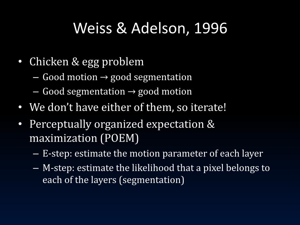
Weiss & Adelson, 1996
• Chicken & egg problem
– Good motion → good segmentation
– Good segmentation → good motion
• We don’t have either of them, so iterate!
• Perceptually organized expectation & maximization (POEM)
– E-step: estimate the motion parameter of each layer
– M-step: estimate the likelihood that a pixel belongs to each of the layers (segmentation)
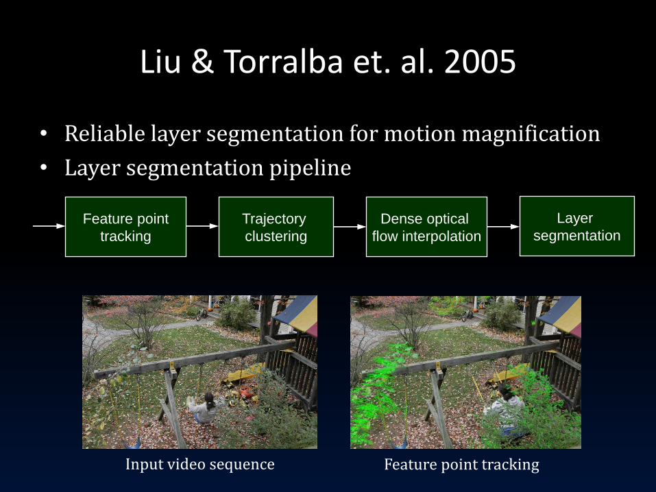
Liu & Torralba et. al. 2005
• Reliable layer segmentation for motion magnification
• Layer segmentation pipeline
Feature point
tracking
Trajectory
clustering
Dense optical
flow interpolation
Layer
segmentation
Input video sequence Feature point tracking

Normalized complex correlation
• The similarity metric should be independent of phase and magnitude
• Normalized complex correlation
tt
t
tCtCtCtC
tCtCCCS
)()()()(
|)()(|),(
2211
2
21
21
Feature point
tracking
Trajectory
clustering
Dense optical
flow interpolation
Layer
segmentation
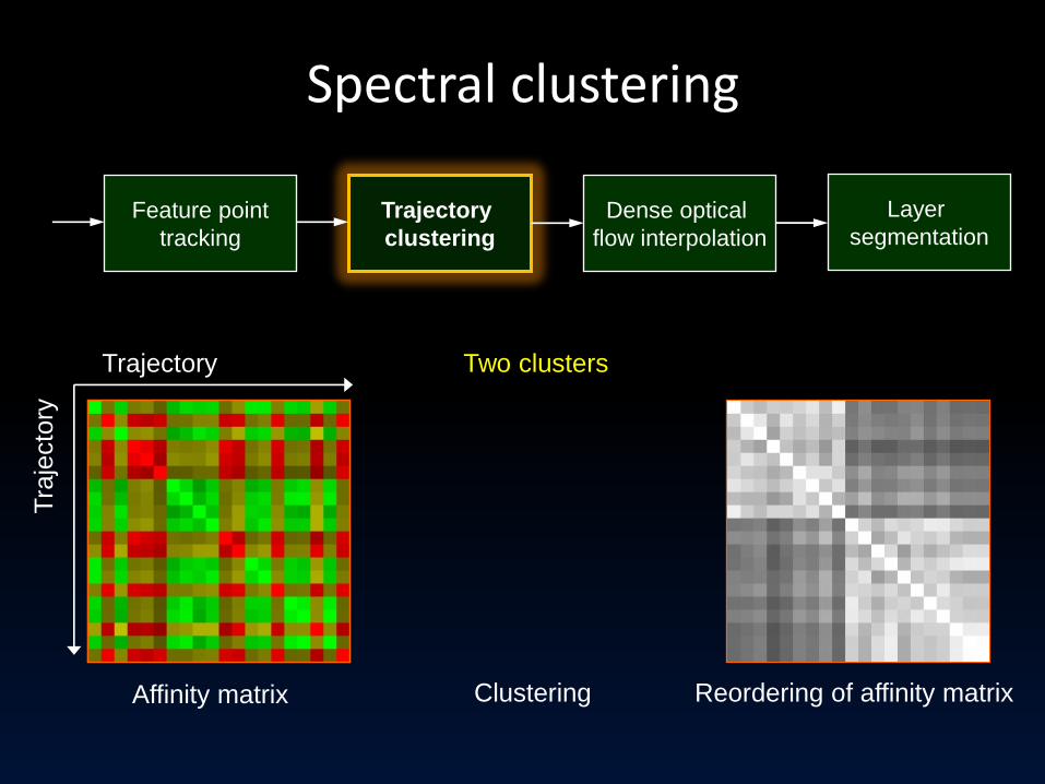
Spectral clustering
Feature point
tracking
Trajectory
clustering
Dense optical
flow interpolation
Layer
segmentation
Affinity matrix Clustering Reordering of affinity matrix
Two clusters Trajectory
Tra
jecto
ry

Clustering results
Feature point
tracking
Trajectory
clustering
Dense optical
flow interpolation
Layer
segmentation

From sparse feature points to dense optical flow fields
Feature point
tracking
Trajectory
clustering
Dense optical
flow interpolation
Layer
segmentation
Flow vectors of
clustered sparse
feature points
Dense optical flow
field of cluster 1
(leaves)
Dense optical flow
field of cluster 2
(swing)
Cluster 1: leaves
Cluster 2: swing
• Interpolate dense optical flow field using locally weighted linear regression

Motion layer assignment
• Assign each pixel to a motion cluster layer, using four cues:
– Motion likelihood—consistency of pixel’s intensity if it moves with
the motion of a given layer (dense optical flow field)
– Color likelihood—consistency of the color in a layer
– Spatial connectivity—adjacent pixels favored to belong the same
group
– Temporal coherence—label assignment stays constant over time
• Energy minimization using graph cuts
Feature point
tracking
Trajectory
clustering
Dense optical
flow interpolation
Layer
segmentation

Segmentation results
Feature point
tracking
Trajectory
clustering
Dense optical
flow interpolation
Layer
segmentation


Generative models
• Learning flexible sprites [Frey & Jojic 2001, 2003]

Content
• Discrete optical flow
• Layer motion analysis
• Contour motion analysis
• Obtaining motion ground truth
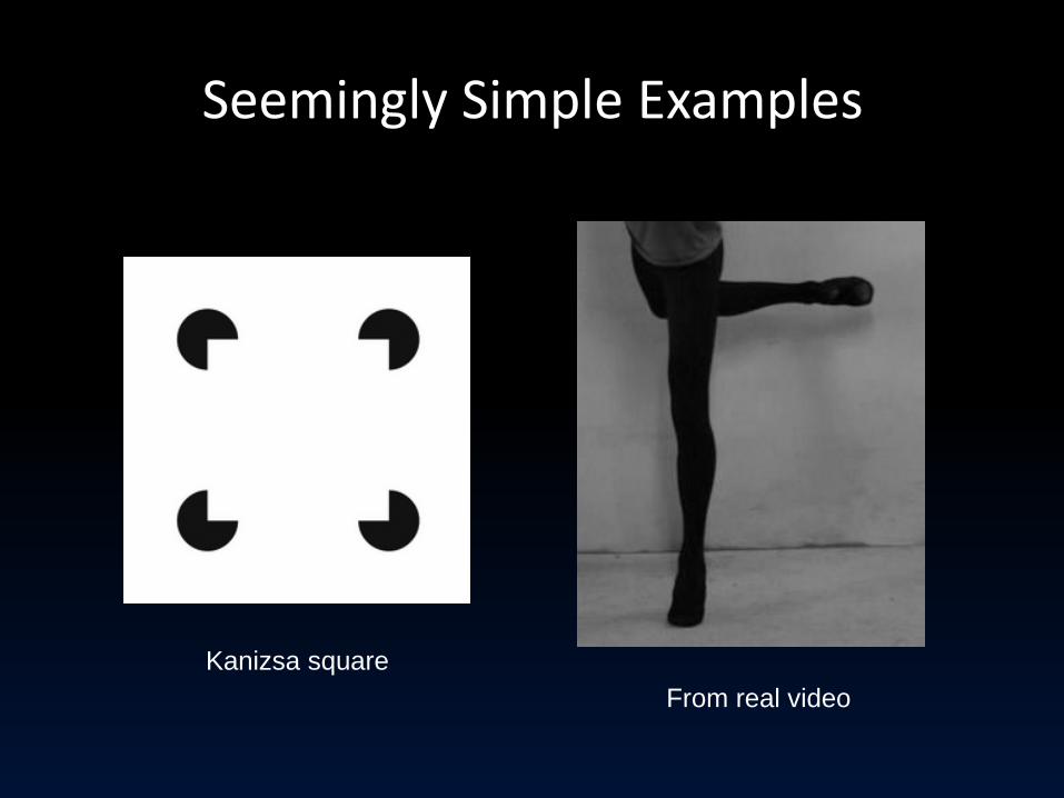
Seemingly Simple Examples
Kanizsa square
From real video

Output from the State-of-the-Art Optical Flow Algorithm
T. Brox et al. High accuracy optical flow estimation based on a theory for warping. ECCV 2004
Optical flow field Kanizsa square

Output from the State-of-the-Art Optical Flow Algorithm
T. Brox et al. High accuracy optical flow estimation based on a theory for warping. ECCV 2004
Optical flow field
Dancer

Optical flow representation: aperture problem
Corners Lines Flat regions
Spurious junctions Boundary ownership Illusory boundaries

Optical Flow Representation
Corners Lines Flat regions
Spurious junctions Boundary ownership Illusory boundaries
We need motion representation beyond pixel level!

Challenge: Textureless Objects under Occlusion
• Corners are not always trustworthy (junctions)
• Flat regions do not always move smoothly (discontinuous at illusory boundaries)
• How about boundaries?
– Easy to detect and track for textureless objects
– Able to handle junctions with illusory boundaries

Analysis of Contour Motions
• Our approach: simultaneous grouping and motion analysis
– Multi-level contour representation
– Junctions are appropriated handled
– Formulate graphical model that favors good contour and motion criteria
– Inference using importance sampling
• Contribution
– An important component in motion analysis toolbox for textureless objects under occlusion
C. Liu, W. T. Freeman and E. H. Adelson. NIPS 2006

Three Levels of Contour Representation
– Edgelets: edge particles
– Boundary fragments: a chain of edgelets with small curvatures
– Contours: a chain of boundary fragments
Forming boundary fragments: easy (for textureless objects)
Forming contours: hard (the focus of our work)

Overview of our system
1. Extract boundary fragments 2. Edgelet tracking with uncertainty.
3. Boundary grouping and illusory boundary 4. Motion estimation based on the grouping

Local Spatial-Temporal Cues for Grouping
Motion stimulus Illusory boundaries corresponding to the groupings (generated by spline interpolation)

Local spatial-temporal cues for grouping: (a) Motion similarity
Motion stimulus
xv
yv
Velocity space
KL( ) < KL( )
The grouping with higher motion similarity is favored

Local spatial-temporal cues for grouping: (b) Curve smoothness
Motion stimulus
The grouping with smoother and shorter illusory boundary is favored

Local spatial-temporal cues for grouping: (c) Contrast consistency
Motion stimulus
The grouping with consistent local contrast is favored

The Graphical Model for Grouping
• Affinity metric 𝜆(𝑆 𝑖, 𝑡𝑖 ; 𝐁, 𝑂) terms
– (a) Motion similarity
exp −𝛼𝐾𝐿𝐾𝐿 𝑁 𝜇11, Σ11 , 𝑁 𝜇21, Σ21
– (b) Curve smoothness
exp −𝛼𝑟 𝑑𝜃
𝑑𝑠
2
𝑟𝑑𝑠
– (c) Contrast consistency
exp −𝑑𝑚𝑎𝑥
2𝜎𝑚𝑎𝑥2 −
𝑑𝑚𝑖𝑛
2𝜎𝑚𝑖𝑛2
• The graphical model for grouping
1b
2b
),( 1111
),( 2121
1b
r
2b
reversibility affinity
11h
12h
21h
22h
1b
2b
no self-intersection
Pr 𝐒; 𝐁, 𝑂 =1
𝑍𝑆 𝜆(𝑆 𝑖, 𝑡𝑖 ;
1
𝑡𝑖=0
𝑁
𝑖=1
𝐁,𝑂)𝛿 𝑆 𝑆 𝑖, 𝑡𝑖 − 𝑖, 𝑡𝑖 ⋅ 𝜓(𝐜𝑗; 𝐁, 𝑂)
𝑀
𝑗=1

Motion estimation for grouped contours
• Gaussian MRF (GMRF) within a boundary fragment
𝜑 𝑣𝑖; 𝑏𝑖 = exp − 𝑣𝑖𝑘 − 𝜇𝑖𝑘𝑇 𝑣𝑖𝑘 − 𝜇𝑖𝑘
−1
𝑖𝑘
exp −1
2𝜎2𝑣𝑖𝑘 − 𝑣𝑖,𝑘+1
2𝑛𝑖−1
𝑘=1
𝑛𝑖
𝑘=1
• The motions of two end edgelets are similar if they are grouped together
𝜙 𝐕 𝑖, 𝑡𝑖 , 𝐕 𝑆 𝑖, 𝑡𝑖 = 1 if 𝑆 𝑖, 𝑡𝑖 = 𝑖, 𝑡𝑖
exp −1
2𝜎2𝐕 𝑖, 𝑡𝑖 − 𝐕 𝑆 𝑖, 𝑡𝑖
2otherwise
• The graphical model of motion: joint Gaussian given the grouping
Pr 𝐕 𝐒; 𝐁 =1
𝑍𝑉 𝜑 𝐯𝑖; 𝐛𝑖 𝜙(𝐕 𝑖, 𝑡𝑖 , 𝐕 𝑆 𝑖, 𝑡𝑖 )
1
𝑡𝑖
𝑁
𝑖
This problem is solved in early work: Y. Weiss, Interpreting images by propagating Bayesian beliefs, NIPS, 1997.

Inference
• Two-step inference – Grouping (switch variables)
– Motion based on grouping (easy, least square)
• Grouping: importance sampling to estimate the marginal of the switch variables – Bidirectional proposal density
𝑞 𝑆 𝑖, 𝑡𝑖 = 𝑗, 𝑡𝑗 ∝1
𝑍𝑞𝜆 𝑆 𝑖, 𝑡𝑖 = 𝑗, 𝑡𝑗 𝜆 𝑆 𝑗, 𝑡𝑗 = 𝑖, 𝑡𝑖
– Toss the sample if self-intersection is detected
• Obtain the optimal grouping from the marginal

Kanizsa Square

Frame 1

Frame 2

Extracted boundary fragments

Optical flow from Lucas-Kanade algorithm
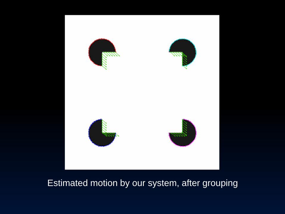
Estimated motion by our system, after grouping
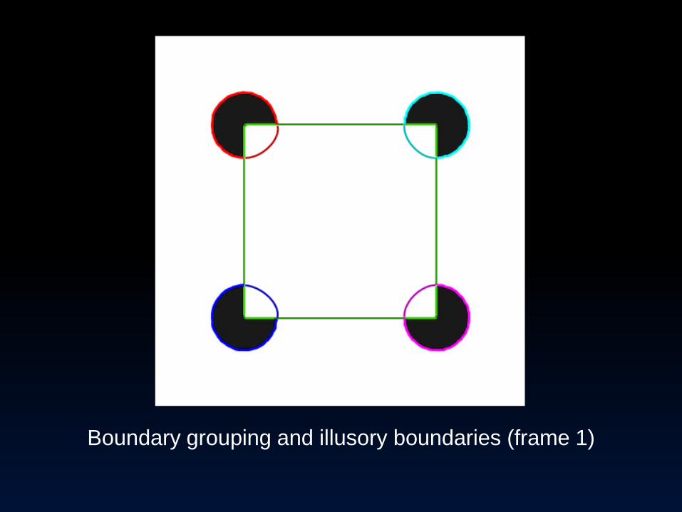
Boundary grouping and illusory boundaries (frame 1)
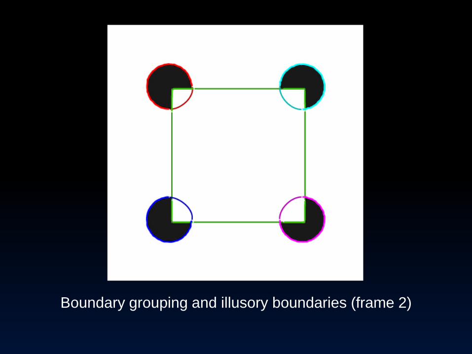
Boundary grouping and illusory boundaries (frame 2)

Rotating Chair

Frame 1

Frame 2

Extracted boundary fragments

Estimated flow field from Brox et al.

Estimated motion by our system, after grouping

Boundary grouping and illusory boundaries (frame 1)
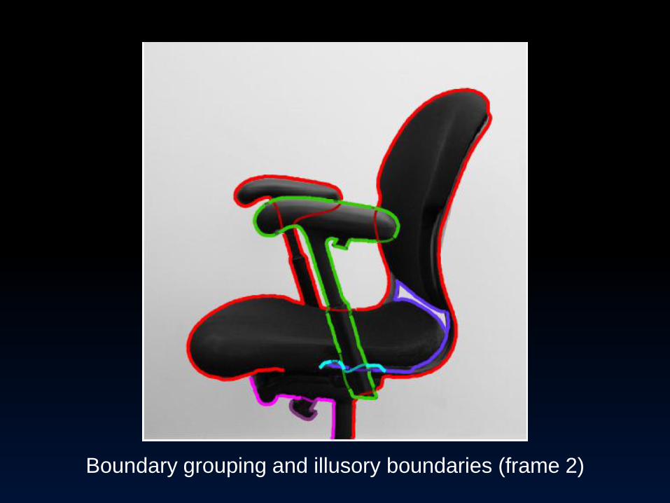
Boundary grouping and illusory boundaries (frame 2)

Content
• Discrete optical flow
• Layer motion analysis
• Contour motion analysis
• Obtaining motion ground truth
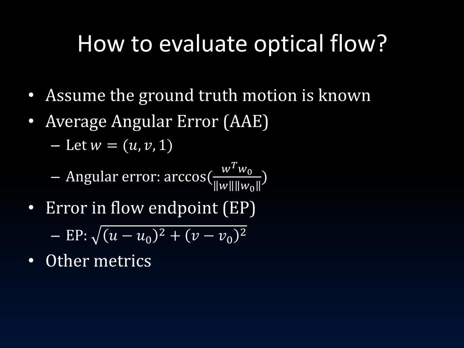
How to evaluate optical flow?
• Assume the ground truth motion is known
• Average Angular Error (AAE)
– Let 𝑤 = (𝑢, 𝑣, 1)
– Angular error: arccos(𝑤𝑇𝑤0
𝑤 𝑤0)
• Error in flow endpoint (EP)
– EP: 𝑢 − 𝑢02 + 𝑣 − 𝑣0
2
• Other metrics

Is optical flow solved
• The AAE (average angular error) race on the Yosemite sequence for over 15 years
#I. Austvoll. Lecture Notes in Computer Science, 2005 *Brox et al. ECCV, 2004.
Yosemite sequence State-of-the-art optical flow* Improvement#

But when optical flow is applied to real-life videos…
Optical flow is far from being solved: – Often fails to capture occluding boundaries correctly
– Puzzles on the right choice of smoothness
Flow visualization
color map A sample sequence State-of-the-art optical flow

Middlebury flow database
Baker et. al. A Database and Evaluation Methodology for Optical Flow. ICCV 2007

Middlebury flow database

Measuring motion for real-life videos
• Challenging because of occlusion, shadow, reflection, motion blur, sensor noise and compression artifacts
• Accurately measuring motion also has great impact in scientific measurement and graphics applications
• Humans are experts in perceiving motion. Can we use human expertise to annotate motion?
[Video courtesy: Antonio Torralba]
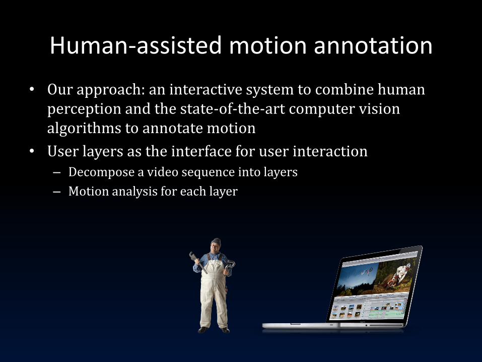
Human-assisted motion annotation
• Our approach: an interactive system to combine human perception and the state-of-the-art computer vision algorithms to annotate motion
• User layers as the interface for user interaction – Decompose a video sequence into layers
– Motion analysis for each layer

Demo: interactive layer segmentation

Demo: interactive motion labeling

Motion database of natural scenes
Color map
Bruhn et al. Lucas/Kanade meets Horn/Schunck: combining local and global optical flow methods. IJCV, 2005

Optical flow is far from being solved
AAE=8.99°
AAE=5.24°
AAE=1.94°
Frame Ground-truth motion Optical flow
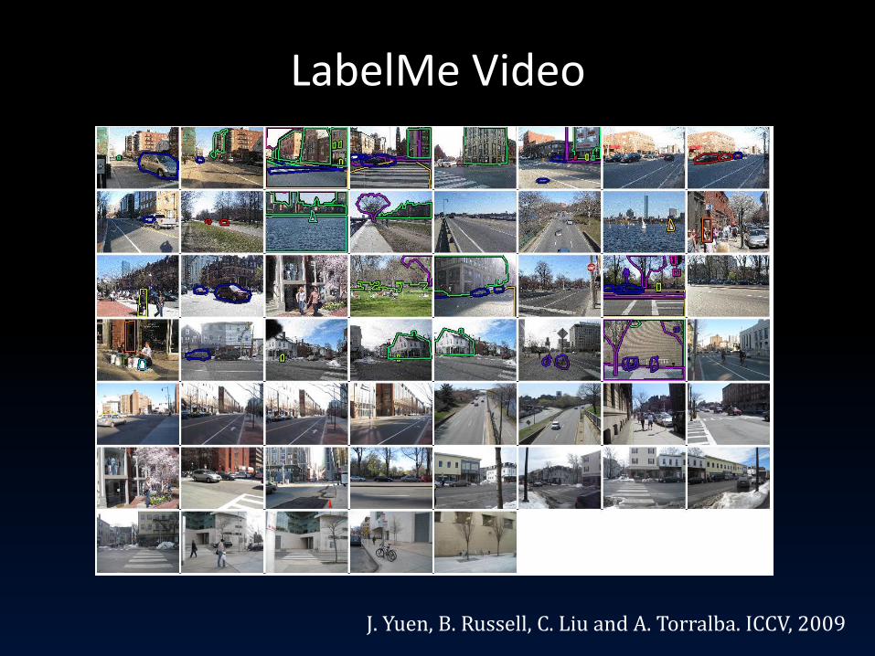
LabelMe Video
J. Yuen, B. Russell, C. Liu and A. Torralba. ICCV, 2009

Summary
• Discrete optical flow matching
– Tracking & motion interpolation
– Belief propagation
• Other representations
– Layer motion analysis
– Contour motion analysis
• Obtaining motion ground truth
– Human assisted motion annotation
u
v