motion transformation by example
TRANSCRIPT

Motion Transformation by Example
by
Eugene Hsu
B. S., University of Washington, Seattle (2002)S. M., Massachusetts Institute of Technology (2004)
Submitted to theDepartment of Electrical Engineering and Computer Science
in partial fulfillment of the requirements for the degree of
Doctor of Philosophy in Computer Science and Engineering
at the
MASSACHUSETTS INSTITUTE OF TECHNOLOGY
September 2008
© Massachusetts Institute of Technology 2008. All rights reserved.
A u th or......... .... ............................................Department of Electrical Engineering and Computer Science
August 29, 2008
Certified by.Jovan PopoviC
Associate ProfessorThesis Supervisor
Accepted by .
MASSACHUSETTS INSTITUTEOF TECHONOLOGY
OCT 2 2 2008
LIBRARIES
t Terry P. OrlandoChairman, Department Committee on Graduate Students
ARCHIVES


Motion Transformation by Example
by
Eugene Hsu
Submitted to the Department of Electrical Engineering and Computer Scienceon August 29, 2008, in partial fulfillment of the
requirements for the degree ofDoctor of Philosophy in Computer Science and Engineering
Abstract
Animated characters bring the illusion of life to feature films, television shows,video games, and educational simulations. However, it is difficult for artists todefine natural and expressive movement. This challenge is compounded by thefact that people are intrinsically sensitive to subtle inaccuracies in human motion.To address this problem, this thesis presents techniques that adjust existing char-acter animations to meet new stylistic or temporal requirements. The proposedmethods learn compact models of the appropriate transformations from examplesprovided by the user. By doing so, they are able to achieve compelling resultswithout significant user effort or skill.
Thesis Supervisor: Jovan PopoviCTitle: Associate Professor


Acknowledgements
First and foremost, I would like to express my gratitude to my thesis supervisor,Dr. Jovan PopoviC. During my time in graduate school, my research interestsand career goals have continuously evolved in some unexpected ways. 'The oneconstant in my academic life was Jovan's support, and I am very thankful for his
guidance and friendship over the years.
This thesis would not have been possible without the contributions of my col-
laborators, Dr. Kari Pulli and Marco da Silva. It was a great honor to have them as
coauthors on my publications. I would also like to acknowledge Dr. Fredo Durand
and Dr. Bill Freeman for their assistance as members of my thesis committee.
I was first introduced to the curious world of computer graphics by my under-
graduate advisor, Dr. Zoran Popovik. Back then, I was an inexperienced student
awestruck by the latest research in the field. Now, ten years later, I have the plea-
sure and privilege of producing that research. I would not be here without Zoran's
initial support.
Over the past several years, I have probably spent more time in the lab than
I have anywhere else. Some of the times were great, and some were just plain
awful. But through it all, I have been able to count on my colleagues in the MIT
Computer Graphics Group for their camaraderie. I've made some great friends
here, and I hope to keep them for the rest of my life.
In every thesis that I've ever read, this section concludes with an obligatory
parental acknowledgement. I always thought that it was terribly trite, and I con-
sidered omitting it entirely. But now that I'm sitting here reminiscing about my
past, I understand where everyone is coming from. So, I'll just keep this simple:
thanks to my mom and my dad for everything.


Contents
1 Introduction1.1 Guided Time Warping
1.2 Style Translation......
1.3 Iterative Motion Warping
2 Background
2.1 Motion Representation
2.2 Motion Generation ....
2.2.1 Blending ......
2.2.2 Database ......
2.2.3 Parametric .....
2.2.4 Physical ......
2.3 Motion Transformation . .2.3.1 Kinematic .....
2.3.2 Physical ......
3 Guided Time Warping
3.1 Motivation .........
3.2 Background ........
3.3 Method ...........
3.3.1 Constraints . ...
3.3.2 Objective ......3.3.3 Optimization . . .3.3.4 Postprocessing . .
3.4 Results ...........
3.4.1 Preservation . ...
13
15
15
15
1717
18
1819
19
20
20
21
21
23
23
2528
28
303234
35
36
.......................
.......................
.......................

3.4.2 Modification..
3.4.3 Performance..
3.5 Discussion .......
4 Iterative Motion Warping
4.1 Background ......
4.2 Method..........
4.2.1 Time Warp...
4.2.2 Space Warp . .
4.2.3 Full Algorithm
4.3 Usage...........
4.4 Results .........
........ 36
........ 38
........ 39
5 Style Translation
5.1 Motivation ........
5.2 Background ........
5.2.1 Content Modeling
5.2.2 Retargeting . . .5.2.3 Implicit Mapping
5.3 Method..........
5.3.1 Representation .5.3.2 Translation Model
5.3.3 Estimation ....
5.3.4 Usage ........
5.3.5 Postprocessing .5.4 Results ..........
5.4.1 Locomotion . . .
5.4.2 Fighting .....
5.5 Summary .........
5.5.1 Discussion . . ..5.5.2 Future Work ...
6 Conclusion
6.1 Implications .......
6.2 Future Work .......
67
68........................... . . . . . . . . . . . . . . . . . . . . . . . . ...........................
. . . . . . . . . . . . . . . . . . .
. . . . . . . . . . . . . . . . . . .
...................
..........
..........
........... . . . . . . . . .
. . . . . . . . . .
. . . . . . . . . .
. . . . . . . . . . . .
............

List of Figures
3-1 Overview of the guided time warping technique. ............ 24
3-2 Comparison of smooth time warping and guided time warping .... 27
3-3 Illustration of the guided time warping algorithm. ............ 30
3-4 Example of guided time warping applied to video sequences. ..... 40
3-5 Sample warps generated by the guided time warping algorithm.. .. 40
4-1 Comparison of dynamic time warping and iterative motion warping. 42
5-1 Visual example of style translation .................... 50
5-2 Overview of our style translation system. ................. 55
5-3 Blending functions for heuristic generalization in style translation. . 61
5-4 Example of style translation in action ................... 64


List of Tables
3.1 Parameters and running times for guided time warping evaluations. 38


Chapter 1
Introduction
Since the invention of the zoetrope, animation has evolved from a visual novelty
into a powerful and method of storytelling. The stylized realities of the original
Walt Disney animations still retain their universal appeal, and their modem Pixar
counterparts continue in this tradition. More recently, highly realistic animations
have found increasing roles in everyday entertainment, from the effects sequences
in modern films to the simulated worlds of interactive games. Beyond entertain-
ment, animated sequences are becoming increasingly common for education and
visualization. They are commonly used in training simulations for sporting, in-
dustrial, and military applications. They can help to illustrate difficult scientific
concepts. From a social perspective, they can cross over cultural and economic
boundaries more easily than their live action equivalents. Animation plays an in-
tegral role in the way people understand the world.
The sophistication of these modem animations comes with a heavy require-
ment for precision and detail. This poses great challenges for the artists that are
involved with such large endeavors. Much research in the computer graphics com-
munity has focused on techniques to simplify these difficult tasks. Laws of physics
have been long been applied to create spectacular imagery, from the undulation of
ocean waves [22] to the formation of entire worlds [66]. But physical phenomena
alone can not tell a story. This is the job of the animated characters, for which
physical laws can only provide limits. Within these limits, and sometimes beyond
them, lie a huge range of actions, intentions, and emotions that require human
insight to specify.

Largely, the construction of character motion remains primitive, often relying
on direct acquisition or meticulous posing. The tools for these methods have cer-
tainly evolved, but the manner in which they are applied does not conceptually
differ from the methods available to animators from decades ago. Commercially
available tools mostly provide interfaces that emulate the posing of mannequins,
and the animation of these poses is nearly identical to the keyframing processes
of the past [80]. Character animation is still a laborious undertaking and its chal-
lenges are compounded by the fact that people are intrinsically sensitive to inac-
curacies in human motion. As a result, many computer graphics researchers have
devised novel methods that learn how to animate from examples. Such techniques
aim to leverage large sets of data acquired from motion capture and archived
hand animation. They have been applied to synthesize new motions using simple
controls such as paths (e.g., [2, 41, 44]), keyframes (e.g., [64]), parameterizations
(e.g., [67, 57]), other motions (e.g., [33]), annotations (e.g., [3]), and so on.
These motion generation approaches often emphasize rapid motion design for
interactive applications. In contrast, the set of motion transformation approaches
emphasize fine adjustment of motions to satisfy new requirements. For instance,
an animator may wish to change an existing motion to have a different style or
meet new spatial or temporal constraints. In this domain, the majority of tech-
niques employ purely kinematic (e.g., [10, 89]) or physical (e.g., [76]) means. How-
ever, relatively few techniques have attempted to learn motion transformations by
example.
The objective of this thesis to address this deficiency. Specifically, we will
demonstrate that surprisingly compact data models can be learned from examples
and applied to useful motion transformation tasks. These models differ signifi-
cantly from those used to generate motion, which must ensure that their internal
models can fully describe the motions that they aim to create. This often limits
their capabilities due to the complexity of character motion. However, transfor-
mation approaches only need to model the desired changes, which allows them
to employ more concise internal representations. We demonstrate this using two
new techniques: guided time warping and style translation.

1.1 Guided Time Warping
Our first technique addresses the fundamental operation of time warping, whichallows users to modify the timing of an animation without affecting its constituentposes. It has many applications in animation systems for motion editing, such asrefining motions to meet new timing constraints or modifying the acting of ani-mated characters. However, time warping typically requires many manual adjust-ments to achieve the desired results. We present a technique, guided time warping,
which simplifies this process by allowing time warps to be guided by a providedreference motion. Given few timing constraints, it computes a warp that both satis-fies these constraints and maximizes local timing similarities to the reference. Thealgorithm is fast enough to incorporate into standard animation workflows. Weapply the technique to two common tasks: preserving the natural timing of mo-tions under new time constraints and modifying the timing of motions for stylisticeffects. This technique is described in Chapter 3.
1.2 Style Translation
Our second technique addresses the task of modifying style. This style translation
technique is capable of transforming an input motion into a new style while pre-serving its original content. This problem is motivated by the needs of interactive
applications which require rapid processing of captured performances. Our solu-
tion learns to translate by analyzing differences between performances of the same
content in input and output styles. It relies on a compact linear time-invariant
model to represent stylistic differences. Once the model is estimated with system
identification, the system is capable of translating streaming input with simple lin-
ear operations at each frame. This technique is described in Chapter 5.
1.3 Iterative Motion Warping
As with many motion generation and transformation approaches, style translationrelies on the ability to find dense temporal correspondences between similar mo-tions. This is a common task for a number of problems involving analysis of time

series, and most techniques that have been applied to this task derive from the
dynamic time warping algorithm [65]. At a high level, this procedure warps the
timeline of one time series to maximize its framewise similarity to another. How-
ever, it fails to account for situations in which signals differ in style. To resolve
this issue, we present iterative motion warping, which identifies correspondences
independently of stylistic differences. We describe this technique in Chapter 4.
Chapter 2
Background
In this chapter, we provide background in character animation. Our goal is to
provide broad overview of the state of the art. For work directly related to our
main contributions, we defer the discussions to the appropriate chapters. We be-
gin in Section 2.1 by describing computational representations of character motion.
Section 2.2 overviews relevant research techniques for motion generation, and Sec-
tion 2.3 describes relevant research techniques for motion transformation.
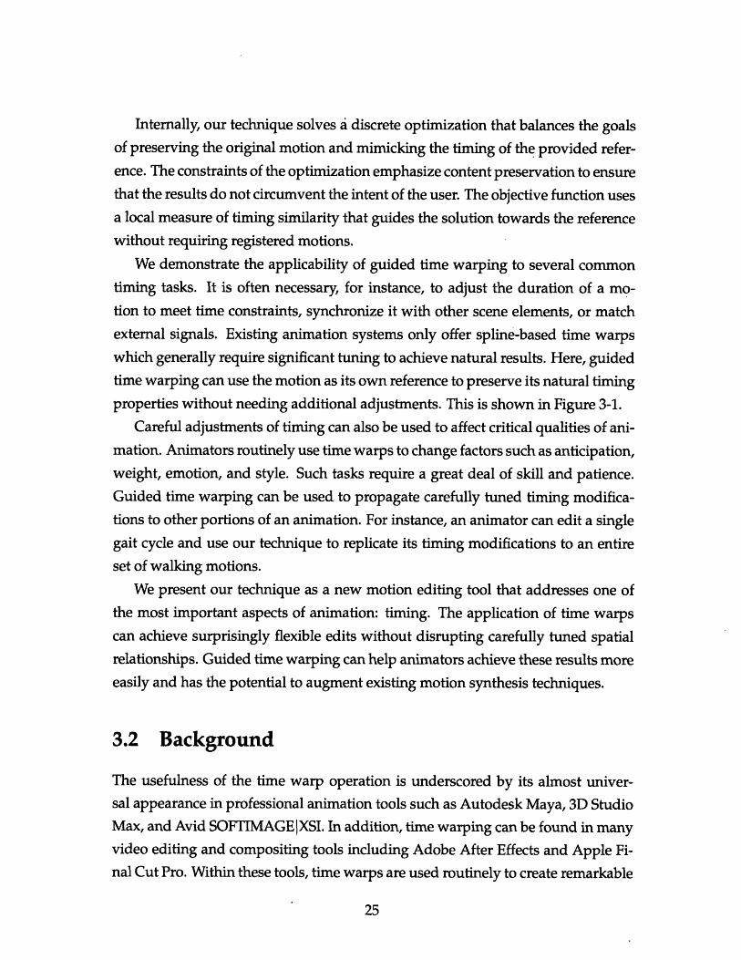
2.1 Motion Representation
The motion of a character is driven by its skeleton, which is a hierarchical structure
of connected joints. Each joint in the skeleton has an associated spatial transfor-
mation relative to its parent joint. At the top of the hierarchy, the transformation
of the root joint is taken relative to the world coordinate system. A typical human
skeleton is rooted at its pelvis joint and branches out to two hip joints and a tho-
rax joint. The hip joints are connected to knee joints, which are connected to ankle
joints, and so on.
The transformation for each joint can be represented as a translation in space
followed by a rotation. Translations are easily represented as three-dimensional
offsets. Rotations may be represented in a number of ways such as Euler angles,
orthogonal matrices, exponential maps [28], or quaternions [72]. These quantities
are encapsulated in a state vector x that specifies the pose of the character at a given
moment in time. A standard human skeleton has about a hundred dimensions.

Given this representation, a motion can be specified as a sequence of poses
(x,x 2, ... , x,). These can be obtained in a number of ways. In hand animation,
an artist typically specifies a set of sparsely timed key poses which are interpo-
lated using splines. This classical technique mimics the traditional cel animation
pipeline [59]. More modern animations have relied increasingly on motion capture
technology, which allows the direct capture of poses from live actors [7].
2.2 Motion Generation
Motion generation approaches seek to construct animation sequences from sparse
constraints. They are often motivated by applications that require interactivity,
rapid prototyping, and simple control. At a high level, such approaches attempt
to capture the space of natural motions. This is a challenging endeavor due to
the complexity of this space. Motion generation techniques attempt to reduce this
complexity in various ways. Blending approaches assume that motions are a lin-
ear combination of a sparse examples (Section 2.2.1). Database approaches assume
that motions are composed of temporally discrete units (Section 2.2.2). Paramet-
ric approaches assume that motions have a compact functional form (Section 2.2.3).
Physical approaches assume that motions are physically consistent (Section 2.2.4).
2.2.1 Blending
The fundamental idea behind blending and morphing approaches is to take a
set of similar motions and interpolate between them to enhance their flexibility.
For instance, given a slow walking motion and a fast walking motion, we can
perform linear interpolation between them to generate a continuum of walking
speeds. Such a scenario was described by Bruderlin and Williams [10]. Rose and
colleagues employed radial basis function interpolation to extend this to multiple
motions [67]. Following the face modeling work of Blanz and Vetter [6], Giese and
colleagues proposed a morphable model for motions [24]. Kovar and Gleicher de-
scribed a way to automatically extract similar sequences from large unstructured
collections of motions [40]. Some researchers also investigated blending models
for interactive motion generation applications [61].

2.2.2 Database
Database approaches take large collections of motion clips and rearrange them to
satisfy new requirements. These techniques are guided by the observation that
motions, while appearing continuous, can be expressed as distinct sequences of
actions. Thus, these actions can be added, removed, and rearranged to produce
new motions. For example, a set of punching, kicking, and walking clips can be
spliced together to form a complete fighting sequence.
Rose and colleagues described a system to splice together parameterized clips
of motion which they call verbs [67]. Sch6dl and colleagues presented a method
to create infinitely long video textures by automatically identifying clip transitions
from long sequences of video. This was brought into the character animation do-
main by researchers who subsequently extended the technique to perform syn-
thesis from constraints such as paths [41, 2, 44], keyframes [64], annotations [3],
control motions [33], low-dimensional inputs [11], and so on. More recently, Lee
and colleagues adopted a database approach for motion generation in complex en-
vironments [46]. Safonova and Hodgins combined database approaches with mo-
tion blending to achieve the best qualities of both types of techniques [68]. McCann
and Pollard [55] and Treuille and colleagues [82] applied reinforcement learning to
perform motion clip selection in interactive contexts. The details of these meth-
ods differ, but they all fundamentally perform discrete optimizations over graph
structures to achieve the desired results.
2.2.3 Parametric
Parametric approaches postulate a generative model of motion. Often times, it is
assumed that motions are drawn from a particular statistical distribution. Li and
colleagues [49] learned a switching linear dynamic system from a set of motions
and used it to randomly synthesize new motions in the style of the input. Brand
and Hertzmann [8] proposed an augmented hidden Markov model to represent
stylistic variations of a particular motion. They used their model to generate mo-
tions in a variety of styles from inputs such as video, scripts, or noise. Vasilescu [85]
built a multilinear model that encoded motions from different people performing
different motions. By doing so, new motions could be generated with independent

adjustment of identity and action. Mukai and colleagues [57] proposed a geosta-
tistical model which allowed for more natural interpolation than existing blending
approaches. Chai and Hodgins described a method to perform sparse keyframe
interpolation from a statistical model of dynamics [12].
2.2.4 Physical
There are a number of techniques that employ the laws of physics to generate re-
alistic motions. In a seminal paper, Witkin and Kass described a method to gener-
ate energy-optimal character motion from sparse constraints using spacetime opti-
mization [88]. Over the years, this technique has been refined to allow better user
control [13], more efficient solution methods [21], and so on. Researchers have also
demonstrated the capabilities of physical techniques for control, drawing heavily
from work in robotics (e.g., [47]). More modem approaches combine physics and
data to generate motions that are both physically correct and natural (e.g., [50]).
Physical correctness, however, can severely limits the creativity of a computer ani-
mator. Our target applications for character animation often involve scenarios that
defy the laws of physics. As such, we limit our discussion to techniques that do
not rely on physical laws.
2.3 Motion Transformation
In contrast to the motion generation approaches described in Section 2.2, motion
transformation approaches adapt provided input motions to novel scenarios, per-
haps by satisfying new spatiotemporal constraints or changing the style of execu-
tion. In theory, all generation approaches could be used for transformation. This
can be done by first extracting the appropriate high-level representation from the
input motion and then using it to drive the internal models of the generation tech-
nique. This indirection, however, comes at the cost of additional complexity and
potential loss of detail. Motion transformation techniques resolve this issue by
modeling the relationship between input and output more directly, thus foregoing
the need for a complex internal representation of motion.

Common transformation techniques are kinematic approaches which model the
input-output relationship directly, often using intuitive parameters, and physical
approaches, which attempt to maintain physical consistency under the desired trans-
formations. The work in this thesis falls into the category of example approaches. We
defer the discussion of such techniques to later chapters.
2.3.1 Kinematic
Kinematic approaches perform simple adjustments to motions to meet new re-
quirements. Bruderlin and Williams described a simple graphic equalizer interface
that allowed the frequency content of motions to be modified [10]. They demon-
strated that this simple technique could produce interesting stylistic effects. In
addition, they described a displacement mapping approach that adjusted motions
to meet new constraints while preserving the original details. A related technique
was presented by Witkin and Popovid [89]. More complex kinematic techniques
have employed spacetime optimization to adapt motions to new characters while
preserving similarity to the original sequence [26, 25, 45]. These approaches fall
into the category of motion retargeting. Kinematic techniques have proven to be
quite effective for these purposes. Some phenomenological models have been de-
rived for certain types of transformations [87], but the general task of performing
abstract transformations is a challenge for most kinematic approaches.
2.3.2 Physical
A number of physical techniques have been proposed that adapt existing mo-
tions to new constraints. Popovie and Witkin described a physically based mo-
tion transformation technique that employed a simplified character representation
to achieve realistic adjustments [63]. Similar techniques were later employed for
adaptation of ballistic motions by Sulejmanpasi6 and Popovid [76] and Majkowska
and Faloutsos [54]. Liu and Popovik presented a technique to transform roughly
keyframed inputs into physically accurate motions [51]. These techniques have all
produced spectacular results for motions that are dominated by physics, such as
ballistic or acrobatic motions. However, physical models are insufficient for more
abstract transformation tasks.


Chapter 3
Guided Time Warping
Time warping is often used to refine motions to meet new timing constraints or
modify the acting of animated characters. However, it typically requires manual
refinement to achieve the desired results. This chapter presents guided time warping,
which simplifies the process of time warping by allowing it to be guided by a
provided reference motion.
3.1 Motivation
A motion that at first appears perfect, whether it is keyframed, captured, or syn-
thesized, will often require further adjustment when it is combined with other
elements in a scene. Modern animation systems provide a number of tools that
transform motions to meet new requirements. The time warp is one such tool that
allows users to adjust the timing of animated characters without affecting their
poses. Its importance follows from the fact that poses often must remain fixed
in later stages of the animation pipeline, since they provide the interface through
which artists collaborate. Any significant spatial changes to a character often ne-
cessitate equally significant changes to the environment, lighting, or camera place-
ment. Timing is one of the few aspects that can be changed without significantly
disrupting workflow.
Typical time warps, however, require significant manual intervention. After
describing high-level synchronization or duration requirements using keytimes,
current animation tools also require users to adjust a curve to achieve the desired
Input Motiona a
Linear Warp
Linear Warp
0 U N!AII 'U am lotAN .. Itl.)j; r
Guided Warpam
IL AI
I ts *it
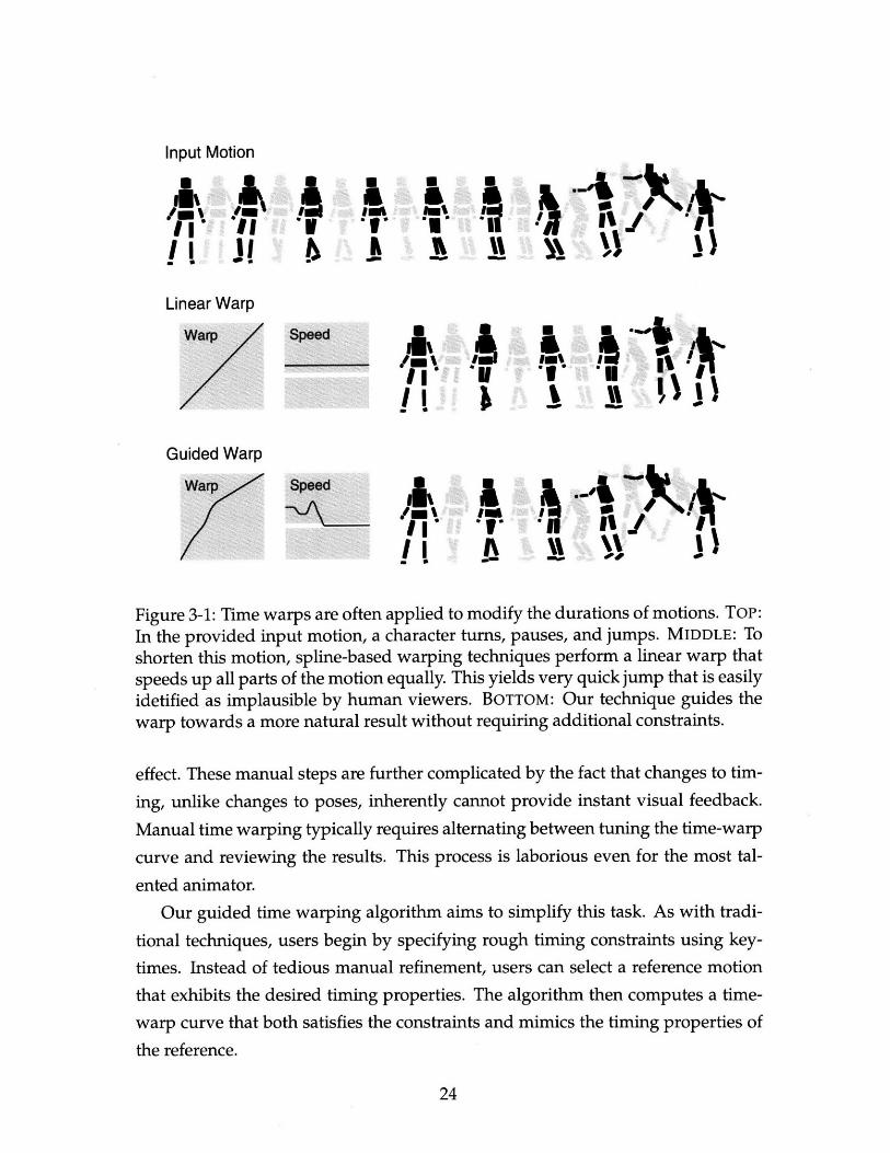
Figure 3-1: Time warps are often applied to modify the durations of motions. ToP:In the provided input motion, a character turns, pauses, and jumps. MIDDLE: Toshorten this motion, spline-based warping techniques perform a linear warp thatspeeds up all parts of the motion equally. This yields very quick jump that is easilyidetified as implausible by human viewers. BOTTOM: Our technique guides thewarp towards a more natural result without requiring additional constraints.
effect. These manual steps are further complicated by the fact that changes to tim-
ing, unlike changes to poses, inherently cannot provide instant visual feedback.
Manual time warping typically requires alternating between tuning the time-warp
curve and reviewing the results. This process is laborious even for the most tal-
ented animator.
Our guided time warping algorithm aims to simplify this task. As with tradi-
tional techniques, users begin by specifying rough timing constraints using key-
times. Instead of tedious manual refinement, users can select a reference motion
that exhibits the desired timing properties. The algorithm then computes a time-
warp curve that both satisfies the constraints and mimics the timing properties of
the reference.
_ I P ::- ... amI . .... r• -
IS
Internally, our technique solves a discrete optimization that balances the goals
of preserving the original motion and mimicking the timing of the provided refer-
ence. The constraints of the optimization emphasize content preservation to ensurethat the results do not circumvent the intent of the user. The objective function usesa local measure of timing similarity that guides the solution towards the reference
without requiring registered motions.
We demonstrate the applicability of guided time warping to several common
timing tasks. It is often necessary, for instance, to adjust the duration of a mo-
tion to meet time constraints, synchronize it with other scene elements, or match
external signals. Existing animation systems only offer spline-based time warps
which generally require significant tuning to achieve natural results. Here, guided
time warping can use the motion as its own reference to preserve its natural timing
properties without needing additional adjustments. This is shown in Figure 3-1.
Careful adjustments of timing can also be used to affect critical qualities of ani-
mation. Animators routinely use time warps to change factors such as anticipation,weight, emotion, and style. Such tasks require a great deal of skill and patience.
Guided time warping can be used to propagate carefully tuned timing modifica-
tions to other portions of an animation. For instance, an animator can edit a single
gait cycle and use our technique to replicate its timing modifications to an entire
set of walking motions.
We present our technique as a new motion editing tool that addresses one of
the most important aspects of animation: timing. The application of time warps
can achieve surprisingly flexible edits without disrupting carefully tuned spatial
relationships. Guided time warping can help animators achieve these results more
easily and has the potential to augment existing motion synthesis techniques.
3.2 Background
The usefulness of the time warp operation is underscored by its almost univer-sal appearance in professional animation tools such as Autodesk Maya, 3D StudioMax, and Avid SOFTIMAGEIXSI. In addition, time warping can be found in manyvideo editing and compositing tools including Adobe After Effects and Apple Fi-nal Cut Pro. Within these tools, time warps are used routinely to create remarkable
results. However, the methods available in these products are basic variants of the
spline-based technique proposed by Witkin and Popovik [89] and thus require a
significant amount of skill and patience.
In the research community, the importance of timing in animation has long
been appreciated. Lasseter's seminal work describes how the slightest timing dif-
ferences can greatly affect the perception of action and intention [43]. More re-
cently, a number of interactive techniques have been proposed to address the tim-
ing problem. Performance-driven animation techniques allow the user to act out
animations using various interfaces (e.g., [16, 81]). Terra and Metoyer present a
technique that is targeted specifically towards time warping [79].
Acting out a motion is a more intuitive way to achieve proper timing, but it
still requires time and skill. McCann and colleagues [56] describe a technique to
compute physically accurate time warps. Our technique aims for greater gener-
ality by relying on data. By doing so, it can capture qualities of animation that
may be difficult or impossible to describe using notions of physical consistency or
optimality. Furthermore, many animations draw their appeal from their stylized
interpretations of realism, which can not be described using physical techniques.
Motion data has been used successfully for many problems in computer ani-
mation. Nonparametric methods assemble short segments of motion data to gen-
erate results that match user specifications, such as desired paths on the ground
or scripts of actions to perform [41, 44, 2, 3]. Of particular relevance to our work
are methods that detect repeatable actions [27] or record timing variations for a
particular action [70]. The timing problem is only partially addressed by these
techniques because they leave the original timing intact at all but a predetermined
set of jump points.
Parametric methods employ different models of time. Blending and morph-
ing methods (e.g., [10, 67]) extrapolate timing using linear combinations of time
warps. Their flexibility is limited by the availability of multiple registered exam-
ples of particular actions. Statistical parameterizations add some flexibility, but
generally involve complex model estimation procedures for carefully constructed
examples or large data sets [8, 49]. By focusing exclusively on timing, our guided
time warping algorithm avoids the need for explicit registration and computation-
ally expensive learning procedures.

Input
Spline
Guided
Figure 3-2: TOP: A user provides an input motion, a set of keytimes, and a ref-erence motion. MIDDLE: A spline-based technique computes a smooth warp thatsatisfies the constraints but ignores the reference motion. BOTTOM: Guided timewarping satisfies the constraints and approximates the timing properties of thereference motion. A spline-based technique would require significant manual re-finement to achieve the same results.
We drew motivation for our work from the speech domain, which has em-
ployed time warps to compress speech signals for the purpose of rapid review
(e.g., [14]). Such techniques perform nonlinear time warps to preserve compre-
hensibility, showing that far higher playback rates can be achieved than with linear
warps. Unfortunately, they would be difficult to apply directly to our task because
of their reliance on specific knowledge about speech understanding. The current
understanding of human motion in computer graphics does not provide the same
helpful guidelines.
Motion
Motion
Motion
Spline
-
Guided

3.3 Method
The guided time warping problem can be stated as follows. A user provides an
input motion, keytimes, and a reference motion. Our technique aims to compute a
time warp that interpolates the keytimes, yielding an output motion that is similar
to both the input and the reference, as shown in Figure 3-2. These two conflicting
goals are reconciled by using different definitions of similarity.
For similarity to the input motion, we enforce constraints on the time warp to
ensure that it preserves the content of the input motion independently of temporal
transformations. This is vital to ensure that our technique does not undermine the
intent of the animator. Our constraint formulation is inspired by dynamic time
warping. We realize these constraints in a discrete formulation (Section 3.3.1).
For similarity to the reference, we define an objective that evaluates the local
similarity of a candidate output motion to the reference. The input and reference
motions will often contain different sequences of actions, precluding the use of
standard correspondence techniques. Instead, we pursue local timing similarities,
in contrast to the global content similarities achieved by dynamic time warping. A
key intuition in our work is the application of a local score function that captures
the timing properties of the reference motion (Section 3.3.2).
The objective function, subject to the previously mentioned constraints, is min-
imized by mapping the problem to a constrained path search. This yields an effi-
cient dynamic programming solution (Section 3.3.3). Simple postprocessing oper-
ations are then applied to achieve the desired results (Section 3.3.4).
3.3.1 Constraints
Time warps can only reproduce poses from the input motion, but their general
application can still yield results that look vastly different. An animator may desire
such effects, but producing them without explicit instructions to do so can lead to
undesirable results. For instance, a general time warp could be used to lengthen
a walk by repeating gait cycles. In earlier prototyping, this may be acceptable.
But when environments are considered, this could mean the difference between
approaching an obstacle and walking straight through it. We realize these concerns
by enforcing constraints that ensure that the content of the input is preserved.

We borrow our constraint formulation from dynamic time warping [65]. This
algorithm is commonly used in computer animation to find global correspondences
between motions (e.g., [67]), but it can also be viewed as a time-invariant similar-
ity measure. The latter perspective offers a convenient and proven way to define
preservation of input content: the result of the any time warp must be identical
to the input motion under the allowed transformations. Since time warps do not
change poses, this can be performed by simply enforcing the constraints of dy-
namic time warping within our optimization.
In the context of our problem, the constraints of dynamic time warping can be
stated as follows. It requires complete time warps, in that they subjectively contain,
the entirety of the input motion. In other words, large blocks of motion should not
be deleted, although it is acceptable to speed through them quickly. It also requires
monotonic time warps, in that they do not loop or reverse time.
We enforce these constraints in a discrete time compression, which we define
as follows. Given a sequence of input frames {xl,... ,xn}, any time warp can be
specified by a subsequence of its frame indices, The identity time warp is defined
by the complete subsequence {1,..., n}. Any subsequence of the identity time
warp yields a monotonic time warp, as its indices must be strictly increasing. Any
monotonic time warp is also complete if it includes 1 and n, and satisfies the prop-
erty that no two adjacent elements differ by more than some integer s. The latter
constraint forces the speed of the output to not exceed s times the original speed;
this prevents the time warp from skipping large blocks of frames. These concepts
are illustrated in Figure 3-3.
Time compressions are only one of many possible time warps. However, we
can reduce other desired warps to compression by suitable transformations. Time
modifications and expansions are reformulated as compressions by upsampling
the input. Backward time warps can be converted to forward time warps by re-
versing the input. Finally, time warps with multiple keytimes can be split into
subproblems of one of the aforementioned cases. As such, we will limit our subse-
quent discussion to the case of compression.

-4
1 3 1 2
4-
Figure 3-3: TOP: An input motion {x 1, X2, X3, X4, X5, X6, X7, X8} is compressedby selecting a subsequence of its frames {xl, X2, X5, X6, x 8} to yield the output{Yl, Y2,Y3, Y4, Y5}. Our constraints require that the first and last frames are re-tained and that no gap between selected frames exceeds a certain amount; here,the maximum gap size is 3. BOTTOM: This output is scored by computing localvelocity and acceleration features and comparing them to equivalently computedvalues in the provided reference. Here, frames {y2, Y3, Y4} are used to computefeature Y3 which is closest to reference feature 2.*
3.3.2 Objective
We aim to compute the quality of a candidate time warp with respect to a pro-vided reference motion. As mentioned before, finding a global correspondencebetween the input motion and the reference motion is generally neither possiblenor desirable. Instead, our technique uses a measure of local similarity to the ref-erence motion. It stems from the following intuition: a pose is an indication ofactivity, and that activity is likely to be executed with a certain timing. For exam-ple, a sitting pose changes more slowly than a jumping pose. The input motionmay already exhibit such canonical timings, but time warps induce changes to thevelocity and acceleration of each pose. Certain poses, such as ones from walking,exhibit natural variations in velocity and acceleration. Other poses, such as onesfrom jumping, exhibit nearly constant acceleration. At a minimum, our objectiveshould capture these variations.

Our solution uses a local score function that computes whether the velocities
and accelerations induced by the time warp resemble those that appear in the refer-
ence motion. In the context of discrete compression, this can be more formally de-fined as follows. Suppose a candidate time warp yields an output of {Yl,...,ym}.
Using finite differences, we compute feature vectors for each frame that encodepose, velocity, and acceleration. The local score of a frame is then defined as its
distance to the nearest equivalently computed feature vector from the reference
motion. The value of the objective function is defined as a sum of local scores:
m-1E(yl,...,ym) = , f (Yi-, Yi, Yi+1). (3.1)
i=2
To compute meaningful velocities and accelerations, we must first choose a
proper representation of poses. We follow Arikan and Forsyth [2] and compute
feature vectors for joint positions in the torso coordinate system of the character.
This transformation allows frames to be represented independently of global posi-
tion and orientation, thus increasing the generality of the local timing models.
The function f(yi-1, Yi, Yi+i) is evaluated as follows. We use the adjacent frames
to compute finite-difference approximations of yi and yi. These terms are assem-
bled into a feature vector yi = [Yi, si, yi]. We perform a k-nearest-neighbor query
on equivalently computed feature vectors for the reference ij. The value of f is
then defined as the average Euclidean distance between the feature vector and its
nearest neighbors:
f (Yi-1, Yi, Yi+1) = k Ai- . (3.2)k iENi
Here, Ni is the set of k-nearest-neigbhors to Yi. For the typical case of smallerreference motions, this can be performed with a linear search. For larger reference
motions, we use an approximate nearest-neighbor data structure [4].One concern that arises here is that of temporal aliasing. Our technique shares
this issue with the dynamic time warping algorithm, as it also employs a discretesignal representation. However, we must take greater precautions, as aliasing arti-facts can be exacerbated by the application of finite-difference estimators. Despitethese concerns, we found in the end that prefiltering the motion with a uniformlow-pass filter was sufficient.

Our decision to avoid higher-order derivatives was motivated by the need
to balance the flexibility and generality of the local timing model. Higher-order
derivatives would more accurately reflect the local properties of a given reference
frame, but they would also be more sensitive to slight differences and provide less
meaningful feature vectors. Ultimately, our choice was made by a combination of
intuition and experimentation.
Before arriving at the current solution, we first tried a purely kinematic ap-
proach that attempted to preserve velocities and accelerations of the input motion.
We found that this strategy works fairly well when the goal is to match the timing
of the input motion as much as possible. However, it can not be applied to more
interesting cases in which the input and reference differ.
We also considered a number of parametric statistical models for the condi-
tional probabilities of velocity and acceleration given a certain pose. We found
that, in practical use, the small sizes of the provided reference motions made it
difficult to produce reliable estimates without overfitting. While various forms of
priors and dimensionality reduction could be applied, we opted for the nearest-
neighbor approach because of its relative simplicity and successful application to-
wards difficult modeling problems in graphics (e.g., [23]) and other domains.
3.3.3 Optimization
Given the constraints and objective function described in the previous sections, we
can define a globally optimal optimization procedure by transforming the problem
into a constrained shortest path search. Note that, as with dynamic time warping,
we define global optimality with respect to a discrete formulation.
We construct vertices that correspond to pairs of input frames that may occur
together in the warped output. This allows us to represent the local terms of the
objective function as edge weights. Formally, we denote each vertex by an ordered
pair of frames (xi, xj), where i < j and j - i < s. We define directed edges connect-
ing vertices (xi, Xj) to (xj, Xk) with weight f(x i, Xj, Xk). This yields a directed acyclic
graph with ns vertices and ns2 edges.

Any path from (xl, xi) to (xj, xn) yields a time warp that satisfies the desired
constraints, and the total weight of such a path is precisely the value of our objec-
tive. For example, suppose the input consists of frames {xl,... ,xs8 }. Then a time
warp {1, 2, 5, 6, 8} corresponds to the path:
(X1,X2) -* (X21,X5) (X5,1X6) -+ (X61,X8).
The edge weights sum to the value of the objective:
f(x 11, x2, x5) + f(x 2, x5, x 6) + f( 5, 6, X 8).
This example is shown in Figure 3-3.
A simple shortest path search will yield the optimal time warp of the input if no
other constraints are given. Since the graph is directed and acyclic, such a search
is linear in the size of the input motion: O(ns2). However, in most cases, we wish
to find the optimal time warp given a target duration m (we show one example
in our results in which this is not the case). This condition can be satisified by
constraining the number of edges in the shortest path search [69]. Specifically, we
want the shortest path from (xl, xi) to (xi, xn) with precisely (m - 2) edges.
The algorithm exploits the fact that the shortest path with p edges must contain
a shortest path of (p - 1) edges. This is formalized by the following recurrence:
cl (xi, xj) = 0, (3.3)
cp(Xj, Xk) = min ci(x, Xj) + f(xi, Xj, xk), (3.4)
where Cp (xi, xj) is the cost of the shortest p-edge path to vertex (xi, xj). The min-
imization proceeds by dynamic programming: first compute all 1-edge shortest
paths, extend those paths to yield 2-edge shortest paths, and so on. The optimal
warp can be recovered by backtracking from the vertex that minimizes Cm-2 (Xj, n).
Equivalently, this optimization can be viewed as a standard shortest path search
on a directed acyclic graph with vertices { (xi, xj)} x {1,...,m - 2} and directed
edges (xi, xj, p) -` (x/, xk, p + 1). Here, the x operator denotes the Cartesian set
product. From this perspective, the time complexity of O(mns2) directly follows.
Note that this is asymptotically identical to dynamic time warping.

So far, we have only described the case when the the first and last frames of
the output are required to match the first and last frames of the input, respectively.
Intermediate constraints may arise when more than two keytimes are specified.
These can be enforced by requiring the path to pass through specific vertices (xi, xj)at specific points p during the optimization procedure, which essentially restarts
the optimization with a modified initialization.
This latter observation can be exploited to achieve a significant, although heuris-
tic, speed improvement to our technique: we first solve a warp on a subsampled
version of the input motion (say, at 5 Hz instead of 30 Hz). The low-resolution so-
lution can then be used to set intermediate keytimes for a full-resolution search.
In practice, we found that this optimization could significantly improve runtimes
with minimal degradation of quality.
3.3.4 Postprocessing
Our technique produces a discrete approximation to the optimal time warp. A di-
rect playback of the selected frames will often yield jumpy results. We resolve this
by applying a moving average filter to the warp, which is then used to resample
the joint angles of the input motion using quaternion slerp interpolation [72].
Time warps, regardless of how they are generated, can modify the frequency
content of the input. For instance, compressions of time can cause a barely per-
ceivable sway to become a nervous jitter. Conversely, expansions of time can yield
overly smoothed results. Such results are sometimes desirable, but they can be
distracting in many applications.
A simple solution to the compression issue is to apply a uniform smoothing to
the output motion, but doing so also dampens important details such as environ-
mental contacts. Such contacts should ideally be identified and incorporated into
a smoothing process. Unfortunately, this is problematic for motion-capture data,
as robust contact detection is difficult and prone to error.
We instead chose to extend the simple solution by applying a local averaging
operation to each frame using a window size proportional to the amount of com-
pression. More specifically, suppose that frame yi of the output is the result of
compressing the original motion by a factor of r (where 1 < r < s). Then we re-
place the frame yi with the average of frames (Yi-r+1,..., Yi+r- 1. Note that the
output is unchanged in the case of no compression (that is, when r = 1). This ap-
proach exploits the observation that undesirable high-frequency details are only
introduced during higher compressions and adapts the amount of smoothing ac-
cordingly. While it can still cause certain details to be lost, we found that it pro-
duces good results in practice.
The expansion issue is more difficult to resolve, as restoring high frequencies
involves hallucinating information absent from the original motion. Existing tech-
niques could be applied to restore detail and texture (e.g., [64]). We chose to
present our results without additional modification because we did not find such
artifacts to be very distracting.
3.4 Results
We demonstrate the application of our technique to editing longer input motions
rather than interpolating closely spaced keytimes. This emulates the typical use of
keyframing tools for time warping: animators first set keytimes to meet duration
or synchronization requirements and then add intermediate keytimes to achieve
the desired results. In these cases, guided time warping can be used to create a
detailed time warp without further user intervention. We envision this to be the
primary use of our technique.
All of our evaluations are performed on motion capture data downsampled
to 30 Hz. We believe our technique to be equally applicable towards high-quality
keyframe animation, but we unfortunately did not have access to such data sets.
Given the difficulty of presenting our results in figure form, we instead refer to
specific examples shown in the accompanying video [32] as V1-V8.
Our first set of results (V1-V5) emphasize how our technique can change the
durations of input motions while preserving their own natural timing properties.
We also show results (V6-V8) in which we modify the timing properies for differ-
ent stylistic effects.

3.4.1 Preservation
Time warping is commonly applied to modify the duration of motions while pre-
serving the natural timing properties of input motion as much as possible. As
described previously, our technique can be applied to this task by providing the
input motion as its own reference. In our video, we compare our preservation
results to those achieved by linear warping. Since duration changes are only spec-
ified with two keytimes, this emulates the behavior of spline-based solutions such
as motion warping [89] when given the same task.
Our first evaluations (V1-V3) test a simple base case for our technique: silence
removal. This commonly used approach for audio can be applied to motions by de-
tecting periods of inactivity. However, a naive implementation of such a technique
would be difficult to tune, as perfectly static motions are very rare. In contrast, our
technique smoothly speeds through low-activity periods in the motion.
These evaluations highlight another desirable aspect of our technique: it man-
ages to preserve the timing of ballistic activities (jumping and falling) without any
prior knowledge of torques, constraints, or gravity. Instead, our objective func-
tion realizes that accelerations during such motions are practically constant and
thus penalizes any temporal deviations. In fact, when presented with the task
of shortening a more challenging motion with only walking and jumping (V4),
the walking portions are sped up extensively while the jumping portions are pre-
served with framewise accuracy. In contrast, a linear scaling of the time axis yields
slightly slower locomotion, but implausible jumps. These results are mirrored for
expansions of the time axis (V5).
3.4.2 Modification
Sometimes time warps are used for the express purpose of deviating from natural
timing. To apply our technique for such tasks, the user simply has to provide a
reference motion with the desired timing properties. Note that our present formu-
lation requires the reference motion to have the same skeleton as the input.
Our first modification evaluation (V6) shows a limited form of style modifica-
tion to a weak boxing sequence. By providing an aggressive sequence of punches
as a reference, our method warps the original input to provide the desired effect

while maintaining its duration. Later in this thesis, we present a similar evaluation
which relies on the availability of matched pairs of motions (Section 5.4.2). Guided
time warping has no such requirement: the provided input and reference motions
can have a different sequence of punches. We also demonstrate the application of
the computed time warp to video footage taken during the capture session. This is
shown in Figure 3-4 and in the accompanying video [32].
While it may be possible to provide canned reference motions, it is often the
case that the only motion available is the one to be modified. In these situations,animators typically must resort to manual warping. Our technique can applied to
simplify this task. We captured a standard locomotion sequence and adjusted asmall segment of it to look more like a limp (V7). This was a slow process, andrepeating it for the rest of the motion would have been very tedious. Instead,we used guided time warping to propagate the timing properties of the modifiedsegment to the remainder of the clip. One important note about this result is thesomewhat unnatural upper body movement in both the reference and the output.This is an unfortunate artifact of any time warping algorithm, since poses in a truelimp differ from those in a normal walk. In spite of this, we chose to include thisexample because it highlights the ability of our technique to work with very shortreference motions.
McCann and colleagues [56] demonstrated a physical approach to solve a sim-ilar task to the previous example using a modification of gravity. While this mayappear to be simpler than our technique, it requires estimating physical parame-ters which are often unavailable for animated characters. Furthermore, it is oftendesirable to have motions that defy physical laws. We demonstrate one such ap-plication by automatically emphasizing jumps using slow motion (V8). For thisexample, we performed a manual time warp to a brief portion of the input motionand used it as a reference. The result shows the remainder of the jumps empha-sized in a similar fashion, despite the fact that the jumps in the input differ signif-icantly from those in the reference. For this evaluation, we did not care how longthe output was, so we ran an unconstrained version of our shortest path search(Section 3.3.2).

Trial n m r s Objective Optimization HeuristicV1 493 280 493 8 1.3s 2.7s 0.17sV2 316 180 316 10 1.7s 1.4s 0.11 sV3 378 180 378 8 1.9s 1.4s 0.14sV4 486 320 486 8 1.0 s 2.6s 0.20sV5 401 150 101 4 0.3s 0.7s 0.06sV6 601 301 301 8 1.3s 3.8s 0.23sV7 573 143 45 8 0.9s 1.8s 0.14sV8 1524 590 91 8 2.5s 0.1s -
Table 3.1: Parameters and running times for our evaluations, measured on a2.4 GHz Pentium 4 PC. For each evaluation, we provide the number of inputframes n, the number of output frames m, the number of reference frames r, andthe frame skip limit s. Separate times are given for the evaluation of the objectivefunction and the optimization procedure. The fast optimization time for V8 is dueto its unconstrained optimization. In the last column, we list optimization timesusing our downsampling heuristic.
3.4.3 Performance
Details of our evaluations are given in Table 3.1. We used k = 3 nearest neigh-
bors for our local score function. The values n, m, and r are frame counts for the
input, output, and reference motions, respectively. The value s is the frame skip
limit, as defined in Section 3.3.1. These frame counts are given after reduction to
compression. The time expansion for V5, for instance, was implemented by first
upsampling a 101-frame input to 401 frames and then compressing it using the
original 101-frame input as the reference. A similar tactic was employed for V6,
V7, and V8, as they required both compressions and expansions of the time axis.
We provide separate timings for the objective evaluation (Section 3.3.2) and
optimization (Section 3.3.3) components of our technique. The former was imple-
mented in C++ using publicly available software [4], and the latter was imple-
mented in MATLAB. The cited timings use our full optimization procedure. We
also applied the heuristic from Section 3.3.3 by downsampling our motions by a
factor of eight. This yields much faster optimization times with little effect on qual-
ity. However, it does not change objective evaluation times because it eventually
performs a pruned search at full resolution.

3.5 Discussion
Time warping is a fundamental motion editing operation that can be used for a
variety of applications. However, time warps must be carefully constructed to en-
sure that the desired results are achieved. Guided time warping provides a simple
alternative to tedious manual specification that can fit seamlessly into existing an-
imation workflows.
One limitation of our technique, as presented, is that it can sometimes be un-
compromisingly automatic. After keytimes and a reference motion are provided,
an animator has little control over the shape of the resulting warp curve. More
keytimes could be specified, but it may also be desirable to add smoothness and
tangent constraints. These would be difficult to encode into guided time warping
due to its local objective. A possible solution might employ motion interpolation
methods (e.g., [39]): by blending between guided warps and spline warps of the
same motion, a user can continuously control of influence of the reference motion
over the final result.
Our results show the preservation of plausible jumps, but it is important to
emphasize that our technique does not explicitly maintain physical consistency.
When this is a priority, other techniques should be applied [56]. A benefit of using
a data model is its capability to handle non-physical animations. Our focus on
animated characters suggests the use of our technique for cartoons and special
effects. However, a broader view of non-physical animation encompasses things
such as camera movement, motion graphics, video footage, and so on. In future
work, we hope to expand upon applications of our technique in these areas.
Ultimately, all time warps are limited by the fact that they can not create or
modify actual postures. No amount of temporal adjustment can convert a slow
walk into a fast sprint, let alone convert a poorly constructed motion into a good
one. As such, we view our technique as complementary to motion synthesis meth-
ods in two regards. From an application perspective, guided time warping is in-
tended for use in later stages of the animation pipeline, when full resynthesis is
often impractical. From a technical perspective, our technique can add new capa-
bilities to existing synthesis techniques by providing more flexible representations
of timing.

Figure 3-4: Guided time warping is not only useful for warping animated se-quences, but other types of signals as well. We used the output of our techniqueto warp video sequences taken during our motion capture session. Here, a weakboxing sequence is made to look more aggressive.
Figure 3-5: Derivatives of time warps for our video evaluations, shown on loga-rithmic scales. The center lines in each plot correspond to unit time, and the limitscorrespond to tenfold slow-motion and fast-forward.
k~ ;i-~; as·a~ -·:···~; ;~:·~'~~:~·-I ~i-~ . :::: I -:B::- ' r~
%-;9:"
k-;
Chapter 4
Iterative Motion Warping
Many techniques in motion generation and transformation rely on dense temporal
correspondences for proper operation. In this section, we describe iterative motion
warping, a correspondence technique specifically designed for the registration of
stylistically different motion signals.
4.1 Background
In a number of scientific domains, it is often necessary to compute dense corre-
spondence between two similar sequences to perform comparisons or modifica-
tions. Computational biologists use these techniques to compare protein sequences
[18], and speech researchers apply them for recognition [65]. The majority of these
techniques operate on discretized sequences using variants of the dynamic time
warping (DTW) algorithm. Briefly, dynamic time warping attempts to perform
correspondence of two motions subject to continuity and monotonicity constraints.
It employs dynamic programming to find the optimal result, which is defined in
terms of framewise similarity. An overview of this algorithm can be found in the
survey article by Myers and Rabiner [58].
Dynamic time warping has been successfully applied to a variety of research
techniques in character animation. Bruderlin and Williams discussed it in the con-
text of motion interpolation [10], and since then the algorithm has become a funda-
mental component of many motion blending techniques (Section 2.2.1). Extensions
have also been proposed to better suit applications in character animation [39].
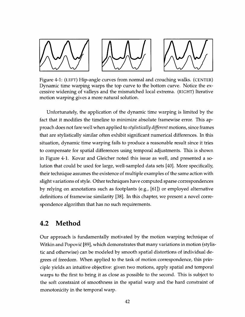
Figure 4-1: (LEFT) Hip-angle curves from normal and crouching walks. (CENTER)Dynamic time warping warps the top curve to the bottom curve. Notice the ex-cessive widening of valleys and the mismatched local extrema. (RIGHT) Iterativemotion warping gives a more natural solution.
Unfortunately, the application of the dynamic time warping is limited by the
fact that it modifies the timeline to minimize absolute framewise error. This ap-
proach does not fare well when applied to stylistically different motions, since frames
that are stylistically similar often exhibit significant numerical differences. In this
situation, dynamic time warping fails to produce a reasonable result since it tries
to compensate for spatial differences using temporal adjustments. This is shown
in Figure 4-1. Kovar and Gleicher noted this issue as well, and presented a so-
lution that could be used for large, well-sampled data sets [40]. More specifically,
their technique assumes the existence of multiple examples of the same action with
slight variations of style. Other techniques have computed sparse correspondences
by relying on annotations such as footplants (e.g., [61]) or employed alternative
definitions of framewise similarity [38]. In this chapter, we present a novel corre-
spondence algorithm that has no such requirements.
4.2 Method
Our approach is fundamentally motivated by the motion warping technique of
Witkin and Popovi' [89], which demonstrates that many variations in motion (stylis-
tic and otherwise) can be modeled by smooth spatial distortions of individual de-
grees of freedom. When applied to the task of motion correspondence, this prin-
ciple yields an intuitive objective: given two motions, apply spatial and temporal
warps to the first to bring it as close as possible to the second. This is subject to
the soft constraint of smoothness in the spatial warp and the hard constraint of
monotonicity in the temporal warp.

In the following discussion, we focus on motions in one dimension and return
to the multidimensional case in Section 4.2.3. Given two motions u and y, itera-
tive motion warping (IMW) finds a correspondence that minimizes the following
objective function:
E(a,b,W) _ (IW(Ua + b) - y1j 2 + IIFa112 + IIGbll 2 . (4.1)
Here, U is diag(u), and Ua + b performs a spatial warp using the scale vector a and
the offset vector b. The warp matrix W performs a nonuniform time warp, which
is constrained to be monotonically increasing. The particular structure of this ma-
trix will be developed in the following section. The terms IFa 112 and II Gb 112 mea-
sure the smoothness of a and b, respectively. More specifically, F and G provide
weighted finite-difference approximations to the first derivatives of a and b, where
the weights are chosen to balance their contribution to the objective.
Iterative motion warping minimizes E by coordinate descent; specifically, it
alternates global optimizations of W and {a, b} until convergence. The discrete
global optimization of W is performed by an algorithm that is conceptually simi-
lar to dynamic time warping [65]. Our formulation differs algorithmically to en-
able interoperability with the continuous optimization of a and b. We detail these
alternating time-warp and space-warp stages in Section 4.2.1 and Section 4.2.2, and
describe their combination in Section 4.2.3.
4.2.1 Time Warp
In this section, we describe the structure and optimization of the warp matrix W,
independently of the scale and offset vectors a and b. We call this component the
time-warp stage. The optimization is performed using dynamic programming, in
a manner very similar to approximate string matching. This problem is defined as
follows. Given two strings p = [pl ... Pm] and q = [q9 ... qn] (where Pi and qjbelong to the same alphabet), find an optimal edit op of p to minimize its difference
from q. Formally stated,
min c c(y(p), qj), (4.2)4)

where Oj(p) is the jth character of the edited p, and c is a cost function, typically
defined to be 0 if its arguments are identical and 1 otherwise. Generally, the edit pis allowed to perform insertions, deletions, and so on. We restrict it to repetition:
it can replace a single character a with ar, 1 < r < k, where k is the repetition
limit. Although this objective differs from those typically given for approximate
string matching, its optimization can be performed with a minor modification of
the dynamic programming recurrences.
This can be used for one-dimensional motion correspondence with several ob-
servations. Given two motions p and q, represented as column vectors, each el-
ement can be considered a character that belongs to the alphabet of reals. A rea-
sonable choice of the cost function c, then, would be the squared difference. Fur-
thermore, the edit function p can be fully parameterized by an integer repetition
vector r, where ri indicates the number of times to repeat Pi. This enables a linear
algebraic representation of the objective:
min |IRp - q 2 -- min 1r2 . p - q (4.3)R r
Here, 1, denotes a column vector of a ones. We call R the repetition matrix; in-
tuitively, it is the result of applying r to the rows of the identity matrix Im. The
constraints of approximate string matching can be rewritten as ri E {1,..., k} and
Ei ri = n.
As described, the algorithm lengthens p to compute the correspondence with q.
It can be applied in more general situations by first lengthening q by s repetitions
of each element. Setting the repetition limit k to s2 emulates the slope constraints of
the standard dynamic time warping algorithm, effectively constraining the slope
of the warp to be between 1/s and s.
We now return to the IMW objective function in Equation (4.1). After length-
ening y, we define p - Ua + b and q = y. It follows from Equation (4.3) that the
described time-warp algorithm performs the desired minimization, giving W as
the repetition matrix R.

4.2.2 Space Warp
The result in the previous section provides a global optimization of E(a, b, W) with
a and b fixed. In the space-warp stage, we optimize E with W fixed. Since the error
function is quadratic in a and b, a unique global optimum is found by zeroing the
first derivative of E with respect to a and b. This yields the following normal
equations, which can be solved efficiently using Gaussian elimination:
UTWTWU + FTF UTWTW a1 ] UT(WTyWTWU WTW + GTG b WTy (4.4)
4.2.3 Full Algorithm
The developments of the previous sections describe the steps of iterative motion
warping for the local minimization of E. We begin by uniformly lengthening y by
the slope limit s, as prescribed by the time-warp stage. After initializing the scale
vector a to 1 and the offset vector b to 0, the time-warp and space-warp stages
are alternated. Convergence follows from the following two observations: since E
only contains quadratic terms, it is lower bounded; since each iteration performs
a global optimization, the value of E cannot increase. In this context, it becomes
clear why it was necessary to produce W in the time-warp stage: without it, the
two stages would be unable to cooperate through a common objective function,
thus precluding any guarantees of convergence.
So far, we have only considered motions in single dimensions. One could use
the algorithm as described on individual degrees of freedom. However, this is
undesirable for many applications, including ours. For instance, when placing lo-
comotions into correspondence, it is important that the legs are synchronized in
the same time frame. Thus, it is often preferable to couple the time warp over all
degrees of freedom. This can be accomplished as follows. Since the time-warp
algorithm only depends on having a cost function, it is replaced by the squared
norm of the frame difference. The space-warp stage is unmodified and used inde-
pendently for each degree of freedom. Correctness follows by parity of reasoning.

4.3 Usage
Iterative motion warping is useful for a variety of techniques that use motion data.
Of course, as it is somewhat unconventional, it is important to explain how one
can substitute it for a standard dynamic time warping algorithm. Given a solution
{a, b, W}, it is unnecessary to retain a and b, as they are just auxiliary terms in
the optimization. The warp matrix W alone encodes the desired correspondence.
Since it is a repetition matrix, we can extract its repetition vector w: this can be
cached from the time-warp stage, or it can be recomputed as diag(WT W). Recall,
however, that this vector encodes a correspondence of u to the s-lengthened ver-
sion of y. To bring it back to normal time, w is divided by the slope limit s. The
resulting w encodes the differential time warp, named as such since integrating it
yields the familiar time-warp curve. Note that w is essentially the dense equiva-
lent of the incremental time-warp parameterization of Park and colleagues [61].
4.4 Results
In this section, we evaluate iterative motion warping. Our data set contained vari-
ous stylized locomotions: normal, limp, crouch, sneak,flap, proud, march, catwalk, and
inverse. Each style was performed at three speeds: slow, medium, and fast. A short
gait cycle was extracted from each motion. Note that iterative motion warping,
like dynamic time warping, requires matched motions to have similar start and
end frames.
Using iterative motion warping, we aligned the extracted motions with the nor-
mal medium walk, with a slope limit of s = 2. We weighted the smoothness of the
scaling and offset terms at 100, but found that these values could be chosen quite
flexibly. For comparison, we also performed alignment with our time-warp al-
gorithm alone and two implementations of dynamic time warping (using Type I
and Type III local constraints [65]). The results of these algorithms for styles with
large pose variations (such as crouch) were different, but equally poor. This was
expected, as stylistically similar frames exhibited large numerical differences. In
contrast, our technique gave consistently better results. A comparison is shown in
Figure 4-1 and in the accompanying video [34].
In use, we found that iterative motion warping took remarkably few iterations
to achieve convergence (typically fewer than ten). It is important to note, however,
that it only guarantees a locally optimal solution. In spite of this, the computed
correspondence is often very good: the first iteration essentially performs dynamic
time warping, and subsequent iterations can only improve the result with respect
to the objective function.
To show the quality of these results, we extracted single gait cycles from the
aligned motions, transformed them to the representation described in Section 5.3.1,
and applied bilinear analysis to separate style and speed [85, 78]. The coordinates
of the motions were then interpolated and extrapolated to allow for continuous
control of style and speed parameters. We looped the gait cycle to create infinite
locomotion. These results are shown in the accompanying video [34].


Chapter 5
Style Translation
Style translation is the process of transforming an input motion into a new style
while preserving its original content. This problem is motivated by the needs of
interactive applications which require rapid processing of captured performances.
Our solution learns to translate by analyzing differences between performances of
the same content in input and output styles. It relies on a novel correspondence
algorithm to align motions and a linear time-invariant model to represent stylistic
differences. Once the model is estimated with system identification, the system is
capable of translating streaming input with simple linear operations at each frame.
5.1 Motivation
Style is a vital component of character animation. In the context of human speech,
the delivery of a phrase greatly affects its meaning. The same can be said for hu-man motion. Even for basic actions such as locomotion, the difference between agraceful strut and a defeated limp has a large impact on the tone of the final an-imation. Consequently, many applications of human animation, such as feature
films and video games, often require large data sets that contain many possible
combinations of actions and styles. Building such data sets places a great burdenon the actors that perform the motions and the technicians that process them.
Style translation alleviates these issues by enabling rapid transformation of hu-man motion into different styles, while preserving content. This allows numerousapplications. A database of normal locomotions, for instance, could be translated
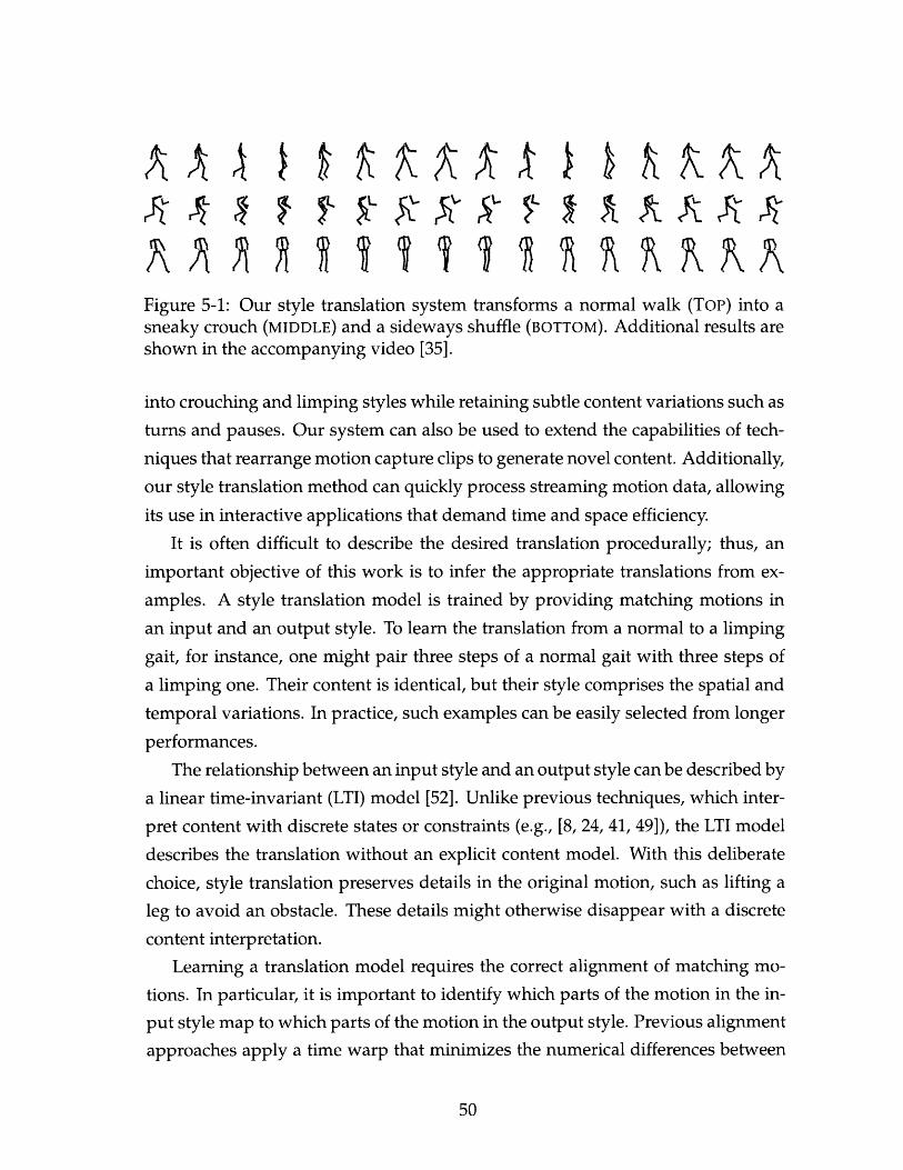
Figure 5-1: Our style translation system transforms a normal walk (TOP) into asneaky crouch (MIDDLE) and a sideways shuffle (BOTTOM). Additional results areshown in the accompanying video [35].
into crouching and limping styles while retaining subtle content variations such as
turns and pauses. Our system can also be used to extend the capabilities of tech-
niques that rearrange motion capture clips to generate novel content. Additionally,
our style translation method can quickly process streaming motion data, allowing
its use in interactive applications that demand time and space efficiency.
It is often difficult to describe the desired translation procedurally; thus, an
important objective of this work is to infer the appropriate translations from ex-
amples. A style translation model is trained by providing matching motions in
an input and an output style. To learn the translation from a normal to a limping
gait, for instance, one might pair three steps of a normal gait with three steps of
a limping one. Their content is identical, but their style comprises the spatial and
temporal variations. In practice, such examples can be easily selected from longer
performances.
The relationship between an input style and an output style can be described by
a linear time-invariant (LTI) model [52]. Unlike previous techniques, which inter-
pret content with discrete states or constraints (e.g., [8, 24, 41, 49]), the LTI model
describes the translation without an explicit content model. With this deliberate
choice, style translation preserves details in the original motion, such as lifting a
leg to avoid an obstacle. These details might otherwise disappear with a discrete
content interpretation.
Learning a translation model requires the correct alignment of matching mo-
tions. In particular, it is important to identify which parts of the motion in the in-
put style map to which parts of the motion in the output style. Previous alignment
approaches apply a time warp that minimizes the numerical differences between

individual poses. This works well for identical or similar styles; however, two mo-
tions in different styles typically contain very different poses. Instead of relying on
heuristic or manual alignment, we employ iterative motion warping, which auto-
matically computes dense correspondences between stylistically different motions
(Chapter 4). The aligned motions are used to estimate the translation model with
system identification techniques.
After estimation, a translation model can receive motions in the input style
and produce motions in the output style (Section 5.3). Without affecting style, our
motion representation removes global position and orientation and exposes time-
invariant stylistic differences. Dense correspondences allow the input-output rela-
tionship to be described at the timing rate of the input, thus guaranteeing perfect
synchrony. The combined use of LTI models and existing postprocessing tech-
niques allow our system to translate with constant latency and memory usage.
There are situations in which specific details of new input motions are not
explored adequately by provided examples, yielding poorly-trained translation
models. We describe a simple and effective heuristic that compensates for this
issue. Additionally, since our model does not account for kinematic interaction
with the environment, the raw output may contain small visual artifacts, such as
feet sliding on the ground. We demonstrate an automatic annotation method that
can be used to correct such artifacts.
5.2 Background
The intent of style translation is most similar to the goal of a style machine [8], a
general parametric representation for encoding style and content in example mo-
tions. After training, a style machine can generate random motions in various
styles, or apply such styles to novel inputs. Similar tasks could also be performed
with non-parametric methods [24] by blending between the examples. Unlike our
approach, however, both methods explicitly model the content in motion, either by
storing examples verbatim, or by learning the parameters of a generative model.
As a result, such models often require explicit frame correspondences to be solved
during the translation process. We describe a more compact and more efficient
translation method that circumvents the need for explicit content modeling.

Our solution draws its main inspiration from retargeting methods, which pre-
serve content, but transform motion to adjust for skeleton size [25], kinematic con-
straints [10, 89], or physics [63]. Style, however, is often difficult to encode in the
procedural forms required by these methods. This was addressed by Amaya and
colleagues [1], who proposed a framework to discover emotional transformations
from data. This work inspired us to model style by examining differences between
example motions.
Statistical analysis of input-output relationships is a fundamental tool in nearly
all areas of science and engineering. In computer graphics, such relationships have
been used to translate styles of line drawings [23], complete image analogies [30],
and so on. Our method is the result of the comprehensive application of these
principles to style translation.
5.2.1 Content Modeling
Database approaches for motion generation assemble short subsequences to syn-
thesize motions that match user specifications, such as a desired path on the ground
or a list of actions to perform [41, 44, 2, 3]. As a result, the output will have the style
of the examples in the database, but the style cannot be applied to new motions.
Pullen and Bregler resolve this problem by retaining low-frequency components
of the input and adding high-frequency texture from the database [64]. This ap-
proach works well when style variations are contained in the high-frequency spec-
trum. However, many types of stylistic variations, such as those between normal,
limping, and crouching gaits, will occur in all bands of the spectrum.
Blending and morphing approaches extrapolate from motion sequences with
linear combinations [67, 24, 36, 39]. Such techniques allow for flexible synthesis of
stylized motion, often with intuitive and tunable parameters. Furthermore, they
can be used effectively for control from intuitive inputs [60]. Applying these ap-
proaches to our problem is more difficult, as style translation is a task of control by
performance, not by constraints or parameters. As a result, such methods would
have to infer the appropriate controls from input, thus adding a level of indirection
that can mask detail and add algorithmic complexity.
Parametric approaches postulate a generative model of motion. Li and col-
leagues use linear dynamic systems [49], while Brand and Hertzmann rely on a
hidden Markov model [8]. Such general models of content would be needed to
enhance a novice dance performance by removing mistakes, such as stumbles. In
our work, we consider those stumbles as part of the content, rather than the style.
Furthermore, if the translation were to map the input onto a sequence of discrete
states, subtle details of the input motion could be lost.
5.2.2 Retargeting
Retargeting methods [10, 89] have been shown to yield compelling and nuanced
motions in interactive applications [45, 71]. In particular, the frequency filtering ap-
proach of Bruderlin and Williams [10] demonstrates that certain stylistic qualities,
such as exaggeration and nervousness, can be manipulated by adjusting frequency
bands with a visual equalizer interface. Unuma and colleagues also propose fre-
quency control of style [83]. These methods rely on procedural definitions of de-
sired properties, or on explicit user input. While procedural formulations could be
derived [62], it is often quicker and easier to define styles by performance.
Style-based inverse kinematics uses such an approach to infer a model of natu-
ral human poses [29]. This method was primarily designed to simplify the process
of creating static human poses, but was also shown to be capable of generating
stylistically consistent animations. Although the model forgoes temporal model-
ing, which is essential for effective style translation, its results emphasize that a
full model of motion content is not required for compelling results.
Our technique bears conceptual similarities to the framework proposed by Amaya
and colleagues for emotional transformations [1]. They also build models of stylis-
tic variation that, after a correspondence process, are able to translate structure
and content. However, they take a significantly different algorithmic approach.
These differences are based on assumptions about the provided examples. While
they aim to build translation models that can, for instance, transfer the quality of
angriness to a kick when provided with an example of an angry drinking motion,
we assume that the examples have greater coverage of the desired space of trans-
lations. As a result, we are able to employ more powerful translation models.

5.2.3 Implicit Mapping
Implicit mapping approaches examine the relationship between two signals to
learn the mapping between them. Dontcheva and colleagues learn the mapping
between a low-dimensional performance and a high-dimensional animation [16].
De La Torre and Black determine the mapping between two high-dimensional mo-
tions by modeling dynamics in a common low-dimensional linear subspace [15].
Jebara and Pentland use Gaussian mixtures to model past-future interaction re-
lationships [37]. In principle, the same learning techniques (asymmetric coupled
component analysis, canonical correlation analysis, and conditional expectation
maximization) could be applied to style translation. We chose to use LTI mod-
els because their importance has led to development of robust and powerful esti-
mation methods [52, 84]. Furthermore, their extensive use in control theory and
modeling of physical processes makes it easier to improve style translation with
better control and more general models. Still, the success of any learning method
is highly dependent proper correspondences.
5.3 Method
Given a sequence of input frames {ut} in the input style, our translation system
computes a sequence of frames {yt} in the output style. In addition, translation
assumes that the input frames are not available as a single batch, but instead ar-
rive one at a time. Our method uses an LTI model to approximate the relationship
between the input and output styles. Once its parameters are estimated from the
training data, the model translates new motions with simple linear transforma-
tions. The output retains the content and the detail of the original input, but differs
in its style of execution. This process is illustrated in Figure 5-2.
The output motion can contain artifacts, either due to a small training set, or
due to interactions between the character and the environment. These can be cor-
rected by a simple but effective postprocess that improves generalization and an-
notates motions for footskate cleanup and other possible applications.

Learning a Translation Model
o
u,0(CDW'0(Dcn0CD
m
3-30
Translating Motions
CD
CD(nCD
0,Io
U+-7Cn3.
0,0
CD':1CD
(PCD
'-.0'n40e
Figure 5-2: An overview of our style translation system. TOP: To build a model,correspondences are first computed for matching example input-output pairs.During representation, the output is warped to the input, and timing informa-tion is added. These frames are used to estimate the translation model. BOTTOM:New frames of input are properly represented and then simulated by the model,yielding output frames. The representation is inverted for synthesis.
5.3.1 Representation
Before modeling, the motions, which are typically encoded in the form of trajecto-ries for each joint angle, are converted into a form that exposes the relevant featuresand meets the technical assumptions of our model. First, our representation un-tangles the spatial and temporal variation between matched motions. Second, ituses differential (relative, instead of absolute) parameters. This is commonly donein statistical time-series modeling to meet the stationarity assumptions of lineartime-invariant models [9].
Time. As described in Section 4.3, iterative motion warping finds a differentialparameterization w of timing differences between motions. This is used to warpexamples in the output style to the time frame of their paired examples in the inputstyle. After this is performed, however, it is necessary to encode the warp so thatit can be reversed during synthesis. This is accomplished by attaching elements ofw to their corresponding frames. Since all of these values are positive, they cor-
-4-4 0
--Iý = -· · ·---

respond to a monotonically increasing timeline. However, there is no guarantee
that the estimated LTI model will produce positive values during synthesis. To
remedy this, we store the logarithm of these values instead, which can be freely
manipulated by our model. Monotonicity is guaranteed during the inversion of
this parameterization because the exponential produces strictly positive values. In
addition, the logarithmic parameterization has the benefit of symmetrizing accel-
erations and decelerations.
Space. Except for the root joint, all joint angles are converted to Cartesian pa-
rameters with the exponential-map parameterization [28]. This mapping ensures
proper manipulation of nonlinear joint-angle quantities by our linear model. The
root joint is treated specially because it encodes a transformation with respect to a
fixed global coordinate system. As such, it is not invariant to ground-plane trans-
lation and vertical-axis rotation. We resolve these problems by encoding the root
position in the ground plane and the orientation around the vertical axis relative
to its position and orientation in the previous frame. The remaining degrees of
freedom, such as height, are preserved. This form is identical to the representa-
tion used by Kovar and Gleicher for coordinate-frame alignment [39]. In addition,
we normalize all degrees of freedom to have zero mean and unit variance across
all frames. This normalization is performed independently for input and output
motions.
5.3.2 Translation Model
Our style translation system uses a linear time-invariant model to explain the rela-
tionship between two motions:
xt+1 = Axt + But + et (5.1)
yt = Cxt + Dut + ft. (5.2)
These difference equations describe the mapping between an input ut and an out-
put yt. The continuous vector xt is the state of the system, and et and ft are white
noise terms that account for measurement errors. The model parameters determine

the mapping between the input and the output; they consist of the dimension ofthe state space, the constant system matrices A, B, C, D, and the constant covariance
matrices of the noise terms. In style translation, the input ut is a d-dimensionalvector representing the degrees of freedom for the input frame t. Similarly, theoutput yt is the (d+1)-dimensional vector for the corresponding frame in the out-put style. The added dimension is the logarithmic time-warp parameter describedin Section 5.3.1.
Our model constrains the input-output mapping to a specific form: it assumesthat each joint is independent of the others. This is motivated by the principles thatguided the design of motion warping techniques [89, 10], which independentlytransform joint-angle curves to meet user-specified constraints. In these applica-tions, the aim was to preserve the content of the input motion, despite transforma-tions needed to comply with the constraints. In our application, the content mustalso be preserved, despite transformations needed to change the style. Similar ap-plications of LTI models for motions [49] and dynamic textures [73] have modeleddegrees of freedom dependently. Such a decision is desirable when deriving gen-erative models, as they do, but this is not our objective. Indeed, the necessarydimensionality reduction would mask detail and introduce unwanted joint corre-lations. The independence assumption circumvents these issues while allowing alldesired dependencies to be translated from the input.
Algorithmically, the benefit of this decision is that it constrains the system ma-trices to a specific block structure, which allows us to decompose the large param-eter estimation task into a set of much smaller ones. In other words, individualsets of system matrices can be independently estimated for each joint and thencombined. By doing so, the number of free model parameters is reduced by an or-der of magnitude, thus simplifying estimation from small data sets. This enablesthe use of powerful parameter estimation techniques which automatically infer thedimension of the state space.
One detail that we have omitted so far is the handling of the timing parame-ter in the output; unlike the joints, there are no directly corresponding degrees offreedom in the input. The appropriate degrees of freedom were chosen by experi-mentation. We found that the best results were achieved by using the differentialposition and orientation of the root.

5.3.3 Estimation
Estimation uses example motions to infer the model parameters: the dimension
of the state space, the system matrices, and optionally (because they are not used
in translation) the noise covariances. This is a classic system identification task
with many standard and robust algorithms [52]. We use the N4SID algorithm [84]
and its implementation in the MATLAB system identification toolbox. Subspace
methods like N4SID consist of two steps. First, the input-output data is used to
estimate the optimal state sequence {xt}. Remarkably, this can be accomplished
without knowing the system matrices. Second, the system matrices are estimated
from the optimal state sequence by solving linear least-squares equations.
For our application, the main advantage of subspace algorithms is ease of use.
The only user parameter is the dimensionality of the state space. Even so, the
choice can be accomplished by inspecting the singular values of a particular ma-
trix. This process is similar to choosing the dimensionality of the subspace ob-
tained by principal component analysis. Automated heuristics are available; those
in MATLAB's N4SID implementation allow estimation of translation models with-
out any user-specified parameters.
System identification routines can provide stable estimates of the dynamical
system matrix A. Practically, this ensures that the translation model recovers quickly
from any undesirable state, as the influence of such states will decay exponentially.
5.3.4 Usage
Using the estimated parameters, our method translates the input by feeding it
through a simulation of the model. This process requires setting the initial state
xo, which is unknown for an arbitrary input motion. To resolve this issue, we set
the initial condition to the steady state xo = 0 and rely on the stability of A to decay
any resulting artifacts. This choice can produce visible artifacts, but they quickly
disappear after several frames. Depending on the application, these frames can
either be ignored or computed heuristically using backward extrapolation.
Given the initial condition, the simulation proceeds in a straightforward man-
ner. As each input frame arrives, it is converted to the proper representation (Sec-
tion 5.3.1): differential root transformations are computed, and degrees of freedom

are normalized using the stored input means and variances. This is fed into the
LTI model, which produces an output. The steps of the representational transfor-
mation are then inverted in the expected manner: reverse the normalization (from
stored output means and variances), accumulate the root transformations, and ex-
ponentiate the log-differential time-warp parameter.
It is important to emphasize that these operations can be performed in a stream-
ing manner. In other words, each frame of input is translated with no lag or looka-
head. Furthermore, the memory requirements are constant, as the state vector
compactly represents all relevant information about previous frames. This obser-
vation may suggest that style translation can be used in online applications, such as
performance-driven animation. Recall, however, that the output of the LTI model
includes a time-warp parameter. The application of this parameter would disrupt
the synchrony between the performer and the output, thus making the method
unsuitable for fully online operation.
This is unfortunately a conceptual limitation of using the time warp. Consider
the task of translating an input style of slow limping to an output style of fast walk-
ing. In this case, a proper style translation, regardless of algorithm, would attempt
to output gait cyclesfaster than they are received. In other words, a live performer
would be incapable of keeping up with the translation! In practice, style transla-
tion might be used for online applications by simply omitting the application of
the time-warp parameter. While this adversely affects the quality of the results, it
may be a reasonable compromise if the input and output styles are similarly timed.
5.3.5 Postprocessing
Given a good training set, our model outputs high-quality motions, but may vio-
late kinematic constraints imposed by the environment. Usually, the most visible
artifact is footskate, which can be corrected by existing methods if the footplants
are annotated [42]. In this section, we describe an efficient classifier that learns
footplant annotations from labeled examples.
A finite training set cannot fully account for the unexpected during a live per-
formance. For these applications, we describe a heuristic that detects unexpectedevents and modifies the output to ensure that they are handled gracefully.

Annotation. We use multiple discriminant analysis (MDA) to build a footplant
classifier from labeled output examples. For a c-class problem, MDA finds the
(c-1)-dimensional projection of labeled feature vectors that maximizes class sepa-
ration [17]. We apply MDA to the estimated state sequences {xt } of the examples,
which are computed during the estimation process (Section 5.3.3). Specifically,
independent one-dimensional MDA projections are computed for each foot, us-
ing classes defined by binary footplant annotations. The projected points in each
class are then modeled by univariate Gaussians, yielding point decision bound-
aries which are stored in the style translation model, along with the MDA projec-
tions, for later use. New footplant classifications are then performed during usage
(Section 5.3.4) by dot products of the current state xt with the stored MDA projec-
tions, followed by comparison with the stored decision boundaries. Note that this
technique makes the naive and incorrect assumption that footplants are indepen-
dent. Despite this fact, it achieves good results in practice.
While our usage of MDA is limited to footplant detection, it can be applied to
other annotation tasks as well. Furthermore, it does not add any lag or lookahead
to the translation process, as it only uses the current state of the LTI model. Note,
however, that the application of postprocessing techniques will often introduce
latency; in the case of footskate cleanup, the added latency is constant.
Heuristic Generalization. Given a motion outside the space explored in the train-
ing examples, our core translation method may output motions with additional
artifacts. The universal solution, of course, is to expand the training set, but this
is often very inconvenient. We describe an extension that uses a simple heuristic
to detect such events and compensates by blending the original input into the out-
put of the LTI model when such events occur. This approach reasons that, if the
translation cannot both preserve the content and translate the style, then it should
prioritize the preservation of the content.
The detection step uses univariate Gaussians (per degree of freedom) to de-
scribe the space of input configurations that can be translated effectively. Recall
that these were also used to normalize each degree of freedom (Section 5.3.1).Given a new value Oi for degree of freedom i, the (Gauss) error function provides

kc=3, kp=2 kc=2, kp=2 kc=1, kp=2 kc=1, kp=4 kc=1, kp=8
Figure 5-3: The effect of kc and kp on the shape of the blend function. All plots areshown on the same scale and centered at the mean.
a reasonable heuristic estimate of translation quality:
z(eirif) 1 er i - i ] p(x;yi,c ) dx. (5.3)
In this expression, the mean yi and the variance q2 define the Gaussian distribution
for the ith degree of freedom. The unit-valued error function z E [0, 1) is then used
to compute a blending weight:
bi(kc,kp) = z(Oi,ji,kcoi)kP. (5.4)
Here, kc defines the confidence that the translation will perform well on unexpected
motions, and kp controls the preference of the blend in ambiguous situations. This is
illustrated in Figure 5-3. We compute the final blend value as b. = maxi bi(kc, kp),which weights the blend of the original input into the output of the LTI model.
5.4 Results
In all our evaluations, we acquired data in a motion capture lab and processedit with standard commercial tools. All motions were recorded at 120 frames persecond and mapped to a skeleton with 35 degrees of freedom.
We applied our system to two style translation tasks. In the first, we trans-lated normal locomotion into a variety of styles. In the second, we translated weakfighting moves into more aggressive ones. These results are shown in the accom-panying video [35].
5.4.1 Locomotion
Our locomotion data set included several styles: normal, catwalk, crouch, limp, and
sideways. The examples consisted of gaits that exhibited variations of speed: slow,
medium,fast, and turning angles: hard left, soft left, straight, soft right, hard right. One
to two minutes of motion were captured for each style. In our experiments, we
found that smaller data sets did not produce reliable models.
Translation models were built from normal to other styles by pairing motion
clips based on their speed and turning angle. These clips were aligned using iter-
ative motion warping, placed into the proper representation, passed to N4SID for
system identification, and so on (Figure 5-2). This entire process was fully auto-
mated, but slow: about an hour, using interpreted MATLAB code. Faster imple-
mentations are possible, but our algorithmic choices for model estimation focused
on quality, not speed. It is the translation performance that is critical.
This objective was certainly achieved. The preprocessing and postprocessing
operations were executed at real-time speeds. Since these operations derive from
proven techniques, their high performance should not be surprising. The more
important figure is the speed of the LTI model simulation. To evaluate this, we
preprocessed a locomotion in batch mode and then fed it through a translation
model with a 98-dimensional state space. Averaged over multiple runs, we ob-
served an effective frame rate of 10000 per second on a 2.4 GHz Pentium 4 PC.
This clearly indicates that style translation models are fast enough for usage in
interactive applications. But more importantly, it implies that they have a negli-
gible performance impact when used in conjunction with existing techniques for
constraint satisfaction, motion blending, and so on.
In our quality evaluations, shown in the accompanying video and in Figure 5-
1, we applied various styles to new normal locomotions. Heuristic generalization
was enabled for all tests using identical parameters. Our first evaluation used
a walking motion with random changes in speed and direction. This motion was
intuitively in the space of the examples. Style translation yielded consistently good
results that exhibited transfer of large-scale content and fine detail.

To emphasize the transfer of details, we edited a locomotion to exaggerate thearm swings. Our results show that this detail was transferred in a stylistically
consistent manner. Finally, we evaluated heuristic generalization by translating
significant deviations from the examples: stepping over an obstacle, ducking, and
limboing. Without heuristic generalization, the results of translation were unpre-
dictable. However, when the input motion returned from the deviation to normal
locomotion, translation recovered very rapidly. This was due to the stability of the
dynamical system matrix, as discussed in Section 5.3.3. With heuristic generaliza-
tion enabled, translation seamlessly blended in the deviation from the input.
5.4.2 Fighting
Our fighting evaluation demonstrates the versatility of style translation. Here, the
goal was to translate punches and kicks of a weak style into an aggressive one.
Our examples consisted of 9 kicks (three low, middle, and high kicks for the right
leg) and 18 punches (three low, middle, and high punches for each arm) in each
style. Using iterative motion warping, matching motions were placed into corre-
spondence using identical parameters to those in the locomotion evaluation. These
motions were used to estimate a style translation model with a 100-dimensional
state space.
We captured a long fighting sequence that contained randomly-ordered punches
and kicks in the weak style. The translation model transformed the sequence into
the aggressive style: the posture was more defensive and the blows were moreforceful. This is shown in Figure 5-4 and in the accompanying video. The trans-lation speed was approximately equal to that for locomotion. This was to be ex-
pected, as the sizes of the state spaces in both evaluations were nearly the same.
5.5 Summary
Our translation system combines proven and novel techniques to produce realistictranslations of style in human motion. The new techniques draw on the observa-tion that stylistic variation is well-approximated by the combination of time warpand linear transformations of individual degrees of freedom. Our iterative mo-

Figure 5-4: A weak punch (TOP) is translated into a more aggressive one (BOTTOM).Notice the differences in posture and speed. This evaluation is also shown in theaccompanying video [35].
tion warping algorithm uses this combination of time and space warps to compute
dense correspondences between stylistically different motions. The alignment pro-
cess is fully automatic, making our algorithm ideal for computing correspondences
between many motions-a task required by many methods in statistical analysis.
Similarly, our translation model combines the time-warp representation with the
linear operations of the LTI model to translate style independently for each joint.
When assembled, these design choices form a fast, effective translation system that
can be used for a variety of applications.
5.5.1 Discussion
Style translation can operate on complex inputs; however, the translation itself
must be relatively simple. The mapping from normal locomotion to limping lo-
comotion, although difficult for humans to describe mathematically, can be com-
pactly parameterized by several matrices. The same can not be said for all situ-
ations in which an input motion maps to an output motion. LTI models would
fail, for instance, to parameterize the complex interaction between dance partners,
as the mapping itself is quite complex [33]. Similarly, one should not expect LTI
models to add or delete choreographic elements [8]. Doing so would contradict
our goal of retaining details in the input motion. For such applications, techniques
with explicit content models are more appropriate.
Despite these apparent limitations, linear time-invariant models can still cap-
ture a rich set of translations significantly beyond the capabilities of linear regres-
sion models. This might at first seem unintuitive given the opaque nature of sys-
tem identification. However, consider that such models can essentially output
linear transformations of the entire history of input frames through the proper
choice of system matrices. This can be done by using the matrices A and B to
shift new values of the input ut into the state xt as if it were a queue of frames.
The system matrices C and D could then be used to perform smoothing, compute
finite-difference estimates of velocity and acceleration, or whatever is necessary
to achieve the desired output. This is an impractical approach due to the limited
availability of example data, but it does serve to illustrate the descriptive capabil-
ities of linear time-invariant models. In use, we believe that these such models
achieve an appealing balance of modeling capability and simplicity.
Our system is intended for applications in which motions are specified by per-
formance. This implies that our present system should not be used to generate
motions from constraints, such as paths or goals. However, we believe that our sys-
tem can be extended to support such constraints by incorporating well-researched
techniques for the control of LTI models [74].
In the present system, the decision to model joints independently has led to the
assumption that the examples of input and output styles share a common skeleton.
This restriction prevents its use in computer-puppetry applications, where an actor
controls a different digital character [75]. This could be resolved in the future by
combining our system with published techniques such as the retargeting approach
of Shin and colleagues [71].
It was not our objective to supplant existing motion synthesis techniques, but
rather to present concepts that could be integrated into past and future work. Iter-
ative motion warping, for instance, could be used to enhance the quality of motion
blending techniques, just as we have adapted the insights from previous work in
this area. In fact, such techniques can be applied directly to remove another tem-
porary limitation of our system, which, as presented, only translates motions into
particular styles. Existing blending techniques can interpolate the output of mul-
tiple translation models to generate arbitrary linear combinations of output styles.

5.5.2 Future Work
Our translation model does not generate physically correct motions. As this is a
common weakness of most blending and statistical methods, it should not be sur-
prising that physically-based approaches could be used in postprocessing. How-
ever, we believe that the simplicity of our model provides additional opportunities
for integration with spacetime techniques [63]. This assertion is supported by the
extensive history of LTI systems in the modeling of dynamic processes [53]. Fur-
thermore, the wealth of available control techniques indicates that our translation
model could also be used in conjunction with robot controllers [20].
This latter connection motivates another fascinating direction that we hope to
pursue in future work. Experimental results in biomechanics continue to provide
a variety of insights about human motion that physics alone cannot explain. By
applying analysis techniques from control theory and other related areas, we hope
to find new insights into the nature of style in human motion.

Chapter 6
Conclusion
In this thesis, we have demonstrated that compact data models can be used effec-
tively to transform character animation for new requirements. Guided time warp-
ing (Chapter 3) encodes the timing qualities of motions using simple local features.
It allows users to adjust motions to meet new timing constraints or modify the
acting of animated characters. Style translation (Chapter 5) encodes stylistic dif-
ferences using a compact linear model, thus enabling rapid motion transformation
without lag or lookahead. Internally, it relies on motion correspondences provided
by our iterative motion warping algorithm (Chapter 4), which itself is based on the
simple model of motion variation proposed by Witkin and Popovie [89].
6.1 Implications
Character animation, due to its complexity, has largely remained a pursuit for
professionals who must often make exacting refinements to achieve the desired
results. In these scenarios, it is often inappropriate to rely on highly automated
motion generation techniques which target simplicity over precision. In contrast,
the motion transformation tools presented in this thesis do not aim to supplant
the talents of these highly skilled users, but rather to augment their abilities bygeneralizing their skillful edits.
Many researchers have aimed to simplify the task of animation for novice artists.
As described in Chapter 2, motion generation techniques allow users to construct
natural motions from sparse high-level constraints. Unfortunately, this automation

often comes at the cost of reduced flexibility. Motion transformation techniques
can greatly expand the applicability of these techniques by providing intuitive ad-
justments of qualities like style and timing.
Motion transformation techniques also have applicability in the domain of in-
teractive character animation. With each new generation of video games, users
demand increasing levels of realism and interactivity. In addition, many video
games are moving towards greater levels of immersion through rudimentary mo-
tion capture devices. Researchers are also proposing novel ways to bring more so-
phisticated motion capture capabilities out of controlled laboratory environments
(e.g., [86]). As such, automated motion generation and transformation techniques
are finding an increasing role in this domain.
Finally, many of the individual techniques and observations in this thesis could
be used to enhance the capabilities of existing methods. For instance, many motion
generation and transformation techniques currently rely on dynamic time warping
as a preprocessing step. Iterative motion warping can be applied immediately to
produce more reliable correspondences in the presence of stylistic variation.
6.2 Future Work
We have demonstrated several novel methods for transforming motions by exam-
ple. In future work, we would like to extend these techniques to other types of
data. Within computer graphics, transformation by example has already been ap-
plied to areas like images [30, 19], vector graphics [31], and meshes [77]. The tem-
poral aspects of our work suggest potential applications towards the analysis and
synthesis of video data. For instance, style translation models could be applied
towards the problem of video transformation. Such a technique would extend
the existing dynamic texture model, which targets video generation [73]. Bennett
and colleagues [5] describe a computational time-lapse video technique that bears
some similarities to guided time warping. They employ ad hoc error metrics to
temporally compress videos while avoiding artifacts such as blurring and alias-
ing. Guided time warping could instead be used to identify the appropriate error
metrics from examples.

Outside of computer graphics, applications such as speech analysis and synthe-
sis could benefit from the models that we have presented. After all, many of the
techniques described in this these have roots in the speech processing domain. As
discussed in Chapter 3, guided time warping bears similarities to nonlinear com-
pression techniques for speech signals. In such applications, time compression is
used to accelerate speech while maintaining comprehensibility [48, 14]. One could
imagine adapting the guided time warping technique to employ models of natural
speech to enhance the capabilities of these techniques. The iterative motion warp-
ing algorithm, described in Chapter 4, can be viewed as a flexible generalization
of the classical dynamic time warping algorithm for connected word recognition.
The idea of alignment under smooth transformations might be useful for speech
applications which must handle "stylistic" variations in timbre, pitch, and accent.
From a user perspective, the concept of transformation by example can prove
useful for a number of tasks that users find easy to demonstrate but difficult to
specify. We have shown two such tasks in this thesis. It is our hope that the work
presented here can lead to simpler and more intuitive design methods in character
animation and beyond.


Bibliography
[1] AMAYA, K., BRUDERLIN, A., AND CALVERT, T. Emotion from motion. InGraphics Interface '96 (May 1996), pp. 222-229.
[2] ARIKAN, O., AND FORSYTH, D. A. Interactive motion generation from ex-amples. ACM Transactions on Graphics 21, 3 (July 2002), 483-490.
[3] ARIKAN, O., FORSYTH, D. A., AND O'BRIEN, J. F. Motion synthesis fromannotations. ACM Transactions on Graphics 22, 3 (July 2003), 402-408.
[4] ARYA, S., MOUNT, D. M., NETANYAHU, N. S., SILVERMAN, R., AND WU,A. Y. An optimal algorithm for approximate nearest neighbor searching fixeddimensions. Journal of the ACM 45, 6 (Nov. 1998), 891-923.
[5] BENNETT, E. P., AND MCMILLAN, L. Computational time-lapse video. ACMTransactions on Graphics 26, 3 (July 2007), 102:1-102:6.
[6] BLANZ, V., AND VETTER, T. A morphable model for the synthesis of 3d faces.In Proceedings of SIGGRAPH 99 (Aug. 1999), Computer Graphics Proceedings,Annual Conference Series, pp. 187-194.
[7] BODENHEIMER, B., ROSE, C., ROSENTHAL, S., AND PELLA, J. The process ofmotion capture: Dealing with the data. In Computer Animation and Simulation(Sept. 1997), pp. 3-18.
[8] BRAND, M., AND HERTZMANN, A. Style machines. In Proceedings of SIG-GRAPH 2000 (July 2000), Computer Graphics Proceedings, Annual Confer-ence Series, pp. 183-192.
[9] BROCKWELL, P. J., AND DAVIS, R. A. Introduction to Time Series and Forecast-ing, 2nd ed. Springer-Verlag, 2002.
[10] BRUDERLIN, A., AND WILLIAMS, L. Motion signal processing. In Proceed-ings of SIGGRAPH 95 (Aug. 1995), Computer Graphics Proceedings, AnnualConference Series, pp. 97-104.
[11] CHAI, J., AND HODGINS, J. K. Performance animation from low-dimensionalcontrol signals. ACM Transactions on Graphics 24, 3 (Aug. 2005), 686-696.

[12] CHAI, J., AND HODGINS, J. K. Constraint-based motion optimization usinga statistical dynamic model. ACM Transactions on Graphics 26, 3 (July 2007),8:1-8:9.
[13] COHEN, M. F. Interactive spacetime control for animation. In Computer Graph-ics (Proceedings of SIGGRAPH 92) (July 1992), pp. 293-302.
[14] COVELL, M., WITHGOTT, M., AND SLANEY, M. Machl: Nonuniform time-scale modification of speech. In Proceedings of 1998 IEEE International Confer-ence on Acoustics, Speech, and Signal Processing (May 1998), pp. 328-338.
[15] DE LA TORRE, F., AND BLACK, M. Dynamic coupled component analy-sis. In IEEE Conference on Computer Vision and Pattern Recognition (Dec. 2001),pp. 643-650.
[16] DONTCHEVA, M., YNGVE, G., AND POPOVIC, Z. Layered acting for characteranimation. ACM Transactions on Graphics 22, 3 (July 2003), 409-416.
[17] DUDA, R. O., HART, P. E., AND STORK, D. G. Pattern Classification, 2nd ed.John Wiley & Sons, Inc., New York, 2000.
[18] DURBIN, R., EDDY, S. R., KROGH, A., AND MITCHISON, G. Biological Se-quence Analysis: Probabilistic Models of Proteins and Nucleic Acids. CambridgeUniversity Press, Cambridge, 1998.
[19] EFROS, A. A., AND FREEMAN, W. T. Image quilting for texture synthesis andtransfer. In Proceedings of SIGGRAPH 2001 (Aug. 2001), Computer GraphicsProceedings, Annual Conference Series, pp. 341-346.
[20] FALOUTSOS, P., VAN DE PANNE, M., AND TERZOPOULOS, D. Compos-able controllers for physics-based character animation. In Proceedings of SIG-GRAPH 2001 (Aug. 2001), Computer Graphics Proceedings, Annual Confer-ence Series, pp. 251-260.
[21] FANG, A. C., AND POLLARD, N. S. Efficient synthesis of physically validhuman motion. ACM Transactions on Graphics 22, 3 (July 2003), 417-426.
[22] FOURNIER, A., AND REEVES, W. T. A simple model of ocean waves. InComputer Graphics (Proceedings of SIGGRAPH 86) (Aug. 1986), vol. 20, pp. 75-84.
[23] FREEMAN, W. T., TENENBAUM, J. B., AND PASZTOR, E. Learning style trans-lation for the lines of a drawing. ACM Transactions on Graphics 22, 1 (Jan. 2003),33-46.
[24] GIESE, M. A., AND POGGIO, T. Morphable models for the analysis and syn-thesis of complex motion patterns. International Journal of Computer Vision 38,1 (June 2000), 59-73.

[25] GLEICHER, M. Retargetting motion to new characters. In Proceedings of SIG-GRAPH 98 (July 1998), Computer Graphics Proceedings, Annual ConferenceSeries, pp. 33-42.
[26] GLEICHER, M., AND LITWINOWICZ, P. Constraint-based motion adaptation.The Journal of Visualization and Computer Animation 9, 2 (Nov. 1998), 65-94.
[27] GOMES, J., VELHO, L., DA SILVA, F. W., AND GOLDENSTEIN, S. K. Motionprocessing using variable harmonic components. In Computer Animation 2000(May 2000), pp. 62-70.
[28] GRASSIA, F. S. Practical parameterization of rotation using the exponentialmap. Journal of Graphics Tools 3, 3 (1998), 29-48.
[29] GROCHOW, K., MARTIN, S. L., HERTZMANN, A., AND POPOVIC, Z. Style-based inverse kinematics. ACM Transactions on Graphics 23, 3 (Aug. 2004),522-531.
[30] HERTZMANN, A., JACOBS, C. E., OLIVER, N., CURLESS, B., AND SALESIN,D. H. Image analogies. In Proceedings of SIGGRAPH 2001 (Aug. 2001), Com-puter Graphics Proceedings, Annual Conference Series, pp. 327-340.
[31] HERTZMANN, A., OLIVER, N., CURLESS, B., AND SEITZ, S. M. Curveanalogies. In Eurographics Workshop on Rendering Techniques 2002 (June 2002),pp. 233-246.
[32] Hsu, E., DA SILVA, M., AND POPOVIC, J. Guided time warping for motionediting. CSAIL Work Product (http://hdl.handle.net/1721.1/41946), 2007.
[33] Hsu, E., GENTRY, S., AND POPOVIC, J. Example-based control of humanmotion. In ACM SIGGRAPH / Eurographics Symposium on Computer Animation(July 2004), pp. 69-77.
[34] Hsu, E., PULLI, K., AND POPOVIC, J. Style translation for human motion.CSAIL Work Product (http:/ /hdl.handle.net/1721.1/42004), 2005.
[35] Hsu, E., PULLI, K., AND POPOVIC, J. Style translation for human motion.CSAIL Work Product (http://hdl.handle.net/1721.1/41945), 2005.
[36] ILG, W., AND GIESE, M. A. Modeling of movement sequences based on hier-archical spatial-temporal correspondence of movement primitives. In Biolog-ically Motivated Computer Vision (Nov. 2002), pp. 528-537.
[37] JEBARA, T., AND PENTLAND, A. Action reaction learning: Automatic visualanalysis and synthesis of interactive behaviour. In International Conference onComputer Vision Systems (1999), vol. 1542, pp. 273-292.

[38] KEOGH, E. J., AND PAZZANI, M. J. Derivative dynamic time warping. InSIAM International Conference on Data Mining (Apr. 2002).
[39] KOVAR, L., AND GLEICHER, M. Flexible automatic motion blending withregistration curves. In ACM SIGGRAPH/Eurographics Symposium on ComputerAnimation (2003), pp. 214-224.
[40] KOVAR, L., AND GLEICHER, M. Automated extraction and parameterizationof motions in large data sets. ACM Transactions on Graphics 23, 3 (Aug. 2004),559-568.
[41] KOVAR, L., GLEICHER, M., AND PIGHIN, F. Motion graphs. ACM Transactionson Graphics 21, 3 (July 2002), 473-482.
[42] KOVAR, L., SCHREINER, J., AND GLEICHER, M. Footskate cleanup for motioncapture editing. In ACM SIGGRAPH Symposium on Computer Animation (July2002), pp. 97-104.
[43] LASSETER, J. Principles of traditional animation applied to 3d computeranimation. In Computer Graphics (Proceedings of SIGGRAPH 87) (July 1987),vol. 21, pp. 35-44.
[44] LEE, J., CHAI, J., REITSMA, P. S. A., HODGINS, J. K., AND POLLARD, N. S.Interactive control of avatars animated with human motion data. ACM Trans-actions on Graphics 21, 3 (July 2002), 491-500.
[45] LEE, J., AND SHIN, S. Y. A hierarchical approach to interactive motion editingfor human-like figures. In Proceedings of SIGGRAPH 99 (Aug. 1999), ComputerGraphics Proceedings, Annual Conference Series, pp. 39-48.
[46] LEE, K. H., CHOI, M. G., AND LEE, J. Motion patches: building blocks for vir-tual environments annotated with motion data. ACM Transactions on Graphics25, 3 (July 2006), 898-906.
[47] LEE, P., WEI, S., ZHAO, J., AND BADLER, N. I. Strength guided motion. InComputer Graphics (Proceedings of SIGGRAPH 90) (Aug. 1990), pp. 253-262.
[48] LEE, S., KIM, H., AND KIM, H. Variable time-scale modification of speechusing transient information. In Proceedings of the 1997 IEEE International Con-ference on Acoustics, Speech, and Signal Processing (1997), vol. 2, pp. 1319-1322.
[49] LI, Y., WANG, T., AND SHUM, H.-Y. Motion texture: A two-level statisticalmodel for character motion synthesis. ACM Transactions on Graphics 21, 3 (July2002), 465-472.
[50] LIU, C. K., HERTZMANN, A., AND POPOVI, Z. Learning physics-based mo-tion style with nonlinear inverse optimization. ACM Transactions on Graphics24, 3 (Aug. 2005), 1071-1081.

[51] LIu, C. K., AND POPOVIC, Z. Synthesis of complex dynamic character motionfrom simple animations. ACM Transactions on Graphics 21, 3 (July 2002), 408-416.
[52] LJUNG, L. System Identification: Theory for the User, 2nd ed. Prentice Hall PTR,1999.
[53] LUENBERGER, D. G. Introduction to Dynamic Systems: Theory, Models, and Ap-plications, 1st ed. Wiley, 1979.
[54] MAJKOWSKA, A., AND FALOUTSOS, P. Flipping with physics: motion edit-ing for acrobatics. In ACM SIGGRAPH / Eurographics Symposium on ComputerAnimation (Aug. 2007), pp. 35-44.
[55] MCCANN, J., AND POLLARD, N. Responsive characters from motion frag-ments. ACM Transactions on Graphics 26, 3 (July 2007), 6:1-6:7.
[56] MCCANN, J., POLLARD, N. S., AND SRINIVASA, S. Physics-based motion re-timing. In ACM SIGGRAPH / Eurographics Symposium on Computer Animation(Sept. 2006), pp. 205-214.
[57] MUKAI, T., AND KURIYAMA, S. Geostatistical motion interpolation. ACMTransactions on Graphics 24, 3 (Aug. 2005), 1062-1070.
[58] MYERS, C. S., AND RABINER, L. R. A comparative study of several dynamictime-warping algorithms for connected word recognition. The Bell SystemTechnical Journal 60, 7 (Sept. 1981), 1389-1409.
[59] O'ROURKE, M. Principles of Three-Dimensional Computer Animation, 3rd ed. W.W. Norton & Company, 2003.
[60] PARK, S. I., SHIN, H. J., KIM, T. H., AND SHIN, S. Y. On-line motion blendingfor real-time locomotion generation. Computer Animation and Virtual Worlds15, 3-4 (2004), 125-138.
[61] PARK, S. I., SHIN, H. J., AND SHIN, S. Y. On-line locomotion generationbased on motion blending. In ACM SIGGRAPH Symposium on Computer Ani-mation (July 2002), pp. 105-112.
[62] PERLIN, K. Real time responsive animation with personality. IEEE Transac-tions on Visualization and Computer Graphics 1, 1 (Mar. 1995), 5-15.
[63] POPOVIC, Z., AND WITKIN, A. P. Physically based motion transformation.In Proceedings of SIGGRAPH 99 (Aug. 1999), Copmuter Graphics Proceedings,Annual Conference Series, pp. 11-20.
[64] PULLEN, K., AND BREGLER, C. Motion capture assisted animation: Texturingand synthesis. ACM Transactions on Graphics 21, 3 (July 2002), 501-508.

[65] RABINER, L. R., AND JUANG, B.-H. Fundamentals of Speech Recognition. Pren-tice Hall, Englewood Cliffs, New Jersey, 1993.
[66] REEVES, W. T. Particle systems - a technique for modeling a class of fuzzyobjects. ACM Transactions on Graphics 2, 2 (Apr. 1983), 91-108.
[67] ROSE, C., COHEN, M. F., AND BODENHEIMER, B. Verbs and adverbs: Multi-dimensional motion interpolation. IEEE Computer Graphics & Applications 18,5 (September - October 1998), 32-40.
[68] SAFONOVA, A., AND HODGINS, J. K. Construction and optimal search ofinterpolated motion graphs. ACM Transactions on Graphics 26, 3 (July 2007),106:1-106:11.
[69] SAIGAL, R. A constrained shortest route problem. Operations Research 16, 1(Jan.-Feb. 1968), 205-209.
[70] SCHODL, A., SZELISKI, R., SALESIN, D. H., AND ESSA, I. Video textures. InProceedings of SIGGRAPH 2000 (July 2000), Copmuter Graphics Proceedings,Annual Conference Series, pp. 489-498.
[71] SHIN, H. J., LEE, J., GLEICHER, M., AND SHIN, S. Y. Computer puppetry: Animportance-based approach. ACM Transactions on Graphics 20, 2 (Apr. 2001),67-94.
[72] SHOEMAKE, K. Animating rotation with quaternion curves. In ComputerGraphics (Proceedings of SIGGRAPH 85) (July 1985), pp. 245-254.
[73] SOATTO, S., DORETTO, G., AND WU, Y. N. Dynamic textures. In InternationalConference on Computer Vision (July 2001), pp. 439-446.
[74] STENGEL, R. F. Optimal Control and Estimation. Dover Books on AdvancedMathematics, New York, NY, 1994.
[75] STURMAN, D. J. Computer puppetry. IEEE Computer Graphics and Applications18, 1 (1998), 38-45.
[76] SULEJMANPASIC, A., AND POPOVIC, J. Adaptation of performed ballisticmotion. ACM Transactions on Graphics 24, 1 (Jan. 2005), 165-179.
[77] SUMNER, R. W., AND POPOVIC, J. Deformation transfer for triangle meshes.ACM Transactions on Graphics 23, 3 (Aug. 2004), 399-405.
[78] TENENBAUM, J. B., AND FREEMAN, W. T. Separating style and content withbilinear models. Neural Computation 12, 6 (June 2000), 1247-1283.

[79] TERRA, S. C. L., AND METOYER, R. A. Performance timing for keyframe ani-mation. In ACM SIGGRAPH / Eurographics Symposium on Computer Animation(July 2004), pp. 253-258.
[80] THOMAS, F., AND JOHNSTON, O. The Illusion of Life: Disney Animation. DisneyEditions, New York, 1981.
[81] THORNE, M., BURKE, D., AND VAN DE PANNE, M. Motion doodles: Aninterface for sketching character motion. ACM Transactions on Graphics 23, 3(Aug. 2004), 424-431.
[82] TREUILLE, A., LEE, Y., AND POPOVIC, Z. Near-optimal character animationwith continuous control. ACM Transactions on Graphics 26, 3 (July 2007), 7:1-7:7.
[83] UNUMA, M., ANJYO, K., AND TEKEUCHI, R. Fourier principles for emotion-based human figure animation. In Proceedings of SIGGRAPH 95 (Aug. 1995),Computer Graphics Proceedings, Annual Conference Series, pp. 91-96.
[84] VAN OVERSCHEE, P., AND DE MOOR, B. Subspace Identification for Linear Sys-tems: Theory, Implementation, Applications. Kluwer Academic Publishers, Dor-drecht, Netherlands, 1996.
[85] VASILESCU, M. A. O. Human motion signatures: Analysis, synthesis, recog-nition. In International Conference on Pattern Recognition (Aug. 2002), vol. 3,pp. 456-460.
[86] VLASIC, D., ADELSBERGER, R., VANNUCCI, G., BARNWELL, J., GROSS, M.,MATUSIK, W., AND POPOVIC, J. Practical motion capture in everyday sur-roundings. ACM Transactions on Graphics 26, 3 (July 2007), 35:1-35:9.
[87] WANG, J., DRUCKER, S. M., AGRAWALA, M., AND COHEN, M. F. The car-toon animation filter. ACM Transactions on Graphics 25, 3 (July 2006), 1169-1173.
[88] WITKIN, A., AND KASS, M. Spacetime constraints. In Computer Graphics(Proceedings of SIGGRAPH 88) (Aug. 1988), pp. 159-168.
[89] WITKIN, A., AND POPOVI(, Z. Motion warping. In Proceedings of SIGGRAPH95 (Aug. 1995), Computer Graphics Proceedings, Annual Conference Series,pp. 105-108.