moving mesh finite element methods for the incompressible navier–stokes...

MOVING MESH FINITE ELEMENT METHODS FOR THEINCOMPRESSIBLE NAVIER–STOKES EQUATIONS∗

YANA DI† , RUO LI† , TAO TANG‡ , AND PINGWEN ZHANG†

SIAM J. SCI. COMPUT. c© 2005 Society for Industrial and Applied MathematicsVol. 26, No. 3, pp. 1036–1056

Abstract. This work presents the first effort in designing a moving mesh algorithm to solve theincompressible Navier–Stokes equations in the primitive variables formulation. The main difficultyin developing this moving mesh scheme is how to keep it divergence-free for the velocity field at eachtime level. The proposed numerical scheme extends a recent moving grid method based on harmonicmapping [R. Li, T. Tang, and P. W. Zhang, J. Comput. Phys., 170 (2001), pp. 562–588], whichdecouples the PDE solver and the mesh-moving algorithm. This approach requires interpolatingthe solution on the newly generated mesh. Designing a divergence-free-preserving interpolationalgorithm is the first goal of this work. Selecting suitable monitor functions is important and isfound challenging for the incompressible flow simulations, which is the second goal of this study.The performance of the moving mesh scheme is tested on the standard periodic double shear layerproblem. No spurious vorticity patterns appear when even fairly coarse grids are used.

Key words. moving mesh method, Navier–Stokes equations, divergence-free-preserving inter-polation, incompressible flow

AMS subject classifications. 65M50, 65N22, 76D05

DOI. 10.1137/030600643

1. Introduction. Many of the modern high resolution methods for solving in-compressible flows use the upwind Godunov approach combined with Chorin’s projec-tion technique [7]; see, e.g., Bell, Colella, and Glaz [1], Brown and Minion [3], E andShu [9], LeVeque [20], and Lopez and Shen [25]. Because the Godunov upwindingapproach stabilizes the computed flows for cell Reynolds numbers where a strictlycentered finite difference scheme would produce spurious oscillations and often in-stability, these Godunov-type methods enable us to make simulations in situationswhere it is not possible to carefully resolve the smallest scales everywhere. With cur-rently available computing machines, such underresolution is often unavoidable. It isnoted that the Godunov-type methods use exact or approximate Riemann solvers thatgreatly complicate the upwind algorithms, making them difficult to implement and togeneralize to more complex systems. To improve this, Kupferman and Tadmor [26]proposed a second order difference method for incompressible flows. Their method isbased on an extension of the classic Lax–Friedrichs scheme introduced for hyperbolicconservation laws [27] and a new discrete Hodge projection. Other state-of-the-artnumerical methods for solving incompressible flow problems include the discontinuousGalerkin method (see, e.g., [24]) and high order schemes (see, e.g., [4, 11, 21]).

∗Received by the editors August 8, 2003; accepted for publication (in revised form) May 3, 2004;published electronically February 3, 2005.

http://www.siam.org/journals/sisc/26-3/60064.html†School of Mathematical Sciences, Peking University, 100871, Beijing, People’s Republic of China

([email protected], [email protected], [email protected]). The research of the firstand second authors was supported in part by the Joint Applied Mathematics Research Institutebetween Peking University and Hong Kong Baptist University. The research of the fourth authorwas supported in part by the special funds for Major State Research Projects and National ScienceFoundation of China for Distinguished Young Scholars.

‡Department of Mathematics, Hong Kong Baptist University, Kowloon Tong, Kowloon, HongKong ([email protected]). The research of this author was supported in part by the HongKong Research Grants Council and the International Research Team on Complex System of ChineseAcademy of Sciences.

1036

MOVING MESH METHODS FOR THE NAVIER-STOKES EQUATIONS 1037

In this work, we study numerical approximations for the incompressible Navier–Stokes equations by using the moving mesh finite element methods. Several movingmesh techniques have been introduced in the past, the most advocated method ofwhich is based on solving elliptic PDEs first proposed by Winslow [36]. Winslow’sformulation requires the solution of a nonlinear Poisson-like equation to generate amapping from a regular domain in a parameter space Ωc to an irregularly shaped do-main in physical space Ω. By connecting points in the physical space correspondingto discrete points in the parameter space, the physical domain can be covered witha computational mesh suitable for the solution of finite difference/element equations.Brackbill and Saltzman [2] formulated the grid equations in a variational form toproduce satisfactory mesh concentration while maintaining relatively good smooth-ness and orthogonality. Their approach has become one of the more popular methodsused for mesh generation and adaptation. In [8], Dvinsky suggests that harmonicfunction theory may provide a general framework for developing useful mesh gen-erators. His method can be viewed as a generalization and extension of Winslow’smethod. However, unlike most other generalizations which add terms or functionalsto the basic Winslow grid generator, his approach uses a single functional to accom-plish the adaptive mapping. The critical points of this functional are harmonic maps.Meshes obtained by Dvinsky’s method enjoy desirable properties of harmonic maps,particularly regularity or smoothness [15, 30].

Motivated by the work of Dvinsky, a moving mesh finite element strategy basedon harmonic mapping was proposed and studied by Li, Tang, and Zhang in [22].The key idea of this strategy is to construct the harmonic map between the physicalspace and a parameter space by an iteration procedure. This procedure is simple,easy to program, and enables us to keep the map harmonic even after a long timeof numerical integration. In our approach, the overall method contains two parts: asolution algorithm and a mesh selection algorithm. These two parts are independentin the sense that the change of the PDEs will affect the first part only.

In this work, using the framework introduced in [22], we develop a moving meshscheme for solving the incompressible Navier–Stokes equations in the primitive vari-ables formulation. To achieve our goal, the main effort is to design a divergence-freeinterpolation which is essential for the incompressible problems. By some careful anal-ysis, we conclude that this can be done by solving linearized, inviscid Navier–Stokes-type equations. Some possible choices of the monitor function will be investigated,which are also essential for the incompressible flow computations.

This paper is organized as follows. In section 2, we briefly describe a standardmixed finite element method for solving the Navier–Stokes equations in the primitivevariables formulation. In section 3, a moving mesh scheme for solving the Navier–Stokes equations is proposed. Since the monitor functions play important roles in themoving mesh implementation, their possible choices are discussed in section 4. Nu-merical experiments demonstrating the efficiency of the proposed numerical methodsare carried out in section 5. Concluding remarks are given in the final section.

2. A mixed finite element method. We consider a two-dimensional incom-pressible Navier–Stokes equation in primitive variables formulation,

∂tu + u · ∇u = −∇p + ν∆u, in Ω,

∇ · u = 0, in Ω,(2.1)

where u = (u, v) is the fluid velocity vector, p is the pressure, and ν is the kinematicviscosity. Without loss of generality, let Ω be the unit square (0, 1) × (0, 1). For ease

1038 YANA DI, RUO LI, TAO TANG, AND PINGWEN ZHANG

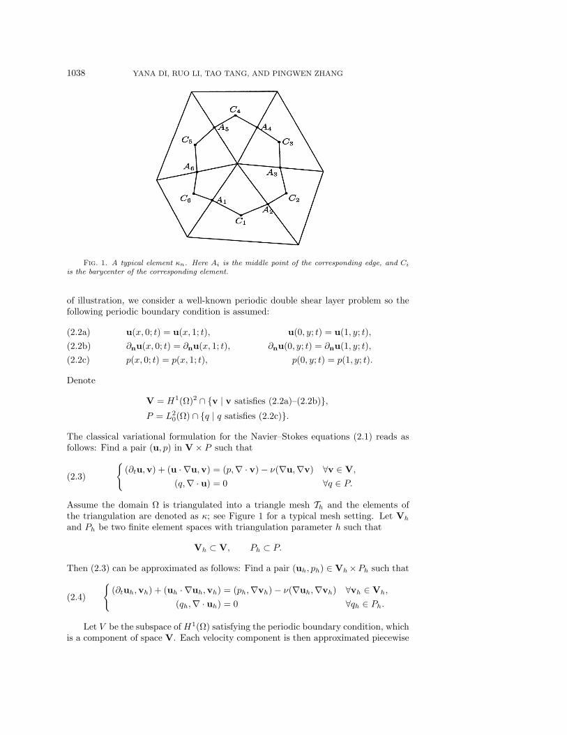
Fig. 1. A typical element κn. Here Ai is the middle point of the corresponding edge, and Ci

is the barycenter of the corresponding element.

of illustration, we consider a well-known periodic double shear layer problem so thefollowing periodic boundary condition is assumed:

u(x, 0; t) = u(x, 1; t), u(0, y; t) = u(1, y; t),(2.2a)

∂nu(x, 0; t) = ∂nu(x, 1; t), ∂nu(0, y; t) = ∂nu(1, y; t),(2.2b)

p(x, 0; t) = p(x, 1; t), p(0, y; t) = p(1, y; t).(2.2c)

Denote

V = H1(Ω)2 ∩ v | v satisfies (2.2a)–(2.2b),P = L2

0(Ω) ∩ q | q satisfies (2.2c).

The classical variational formulation for the Navier–Stokes equations (2.1) reads asfollows: Find a pair (u, p) in V × P such that

(∂tu,v) + (u · ∇u,v) = (p,∇ · v) − ν(∇u,∇v) ∀v ∈ V,

(q,∇ · u) = 0 ∀q ∈ P.(2.3)

Assume the domain Ω is triangulated into a triangle mesh Th and the elements ofthe triangulation are denoted as κ; see Figure 1 for a typical mesh setting. Let Vh

and Ph be two finite element spaces with triangulation parameter h such that

Vh ⊂ V, Ph ⊂ P.

Then (2.3) can be approximated as follows: Find a pair (uh, ph) ∈ Vh×Ph such that(∂tuh,vh) + (uh · ∇uh,vh) = (ph,∇vh) − ν(∇uh,∇vh) ∀vh ∈ Vh,

(qh,∇ · uh) = 0 ∀qh ∈ Ph.(2.4)

Let V be the subspace of H1(Ω) satisfying the periodic boundary condition, whichis a component of space V. Each velocity component is then approximated piecewise


linearly on every triangle element, which forms a continuous finite element spaceVh ⊂ V . Denote Vh = (Vh)2. This is an order-one approximation for the velocity.For the pressure p, we adopt the piecewise constant finite element space Ph ⊂ P onthe dual mesh of Th. Thus, the a priori error estimates of such an approximation areknown (see, e.g., [13, 14]),

‖u − uh‖1,Ω + ‖p− ph‖0,Ω ≤ C1h(|u|2,Ω + |p|1,Ω).(2.5)

Furthermore, if Ω is convex, then the above result can be further improved to

‖u − uh‖0,Ω ≤ C2h2(|u|2,Ω + |p|1,Ω).(2.6)

In the temporal direction, a multistep Runge–Kutta scheme will be employed. Ac-cording to E and Liu [11], for a convection-dominated problem (which is our interest),the order of the Runge–Kutta scheme should be at least three in order to guaranteethe numerical stability. In this work, a three-step Runge–Kutta scheme is used,∀(vh, qh) ∈ Vh × Ph:

1. Stage 1:

⎧⎪⎨⎪⎩

(u1h − u

(n)h

∆t/3,vh

)+ (u

(n)h · ∇u

(n)h ,vh) = (p1

h,∇vh) − ν(∇u1h,∇vh),

(∇ · u1h, qh) = 0.

(2.7)

2. Stage 2:

⎧⎪⎨⎪⎩

(u2h − u

(n)h

∆t/2,vh

)+ (u1

h · ∇u1h,vh) = (p2

h,∇vh) − ν(∇u2h,∇vh),

(∇ · u2h, qh) = 0.

(2.8)

3. Stage 3:

⎧⎪⎪⎨⎪⎪⎩

(u

(n+1)h − u

(n)h

∆t,vh

)+ (u2

h · ∇u2h,vh) = (p

(n+1)h ,∇vh) − ν(∇u

(n+1)h ,∇vh),

(∇ · u(n+1)h , qh) = 0.

(2.9)

It is noted that the above scheme needs only one set of intermediate variables. More-over, the viscosity terms are treated implicitly and the nonlinear terms are treatedexplicitly. It is known (see, e.g., [11]) that for problems with very small viscosities(again, as is the case of our interest) an explicit Runge–Kutta treatment for the vis-cosity terms is acceptable for time marching. However, if there is a thin internallayer, as in our numerical examples, then the mesh needs to be highly adapted toresolve such a layer, which will affect the choice of time step restriction of an explicitmethod. To be more specific, let us take a one-dimensional viscous Burgers equationwith layer width O(ε) as an example. Roughly speaking, the time-step restrictionshould satisfy ∆t ∼ min∆tCFL,∆tvis, where ∆tCFL is the standard CFL conditionand ∆tvis is the viscous time step in the layer regions. The viscous time step is defined


by ∆tvis ∼ ∆x2/ε, where ∆x is the mesh diameter in the layer region. For the viscousBurgers equation with layer size O(ε), this implies that

∆x ∼ c1ε.(2.10)

It follows that if the proportional constant c1 is sufficiently small, then the time-steprestriction of an explicit method will be determined by the viscous time step ratherthan the CFL condition. In moving mesh computations, the proportional constant c1in (2.10) may be very small due to the mesh-moving effect. As a result, with anexplicit scheme the (very small) viscous time step has to be used. In this case, themethods of handling the extremely small time steps include the use of locally varyingtime steps (see, e.g., [31]) or an implicit treatment of the viscous terms. In this work,the latter method is employed, which is quite standard in handling the incompressibleNavier–Stokes equations; see, e.g., [12, 19].

3. A moving mesh strategy. At time t = tn+1, a finite element solution

(u(n+1)h , p

(n+1)h ) is obtained using the method described in the last section. Now the

question is how to obtain a new mesh T (n+1)h using this new solution and the old

mesh T (n)h . To this end, we extend the method proposed in [22, 23] to deal with the

incompressible flow problems in this section.We follow the framework given in [22, 23] but highlight the main differences

and difficulties due to the incompressibility constraint. Roughly speaking, the meshgeneration scheme consists of the following three steps:

• Step 1: Solve the elliptic system

∇x

(m∇x

ξ)

= 0(3.1)

together with the boundary conditions

ξ(0, y) + (1, 0)T = ξ(1, y), ξ(x, 0) + (0, 1)T = ξ(x, 1),(3.2a)

∂nξ(0, y) = ∂n

ξ(1, y), ∂nξ(x, 0) = ∂n

ξ(x, 1),(3.2b)

where the function m in (3.1) is a monitor function which is, in general,

dependent on the solution (u(n+1)h , p

(n+1)h ). We assume m is given here; its

choice is crucial to the moving mesh method and is discussed in section 5.• Step 2: Denote the initial (fixed uniform) mesh in the logical domain as Tc

(with nodes A(0)) and the new logical mesh obtained by solving (3.1)–(3.2)as T ∗

c (with nodes A∗). Their difference,

δA = A(0) −A∗,(3.3)

is used to determine the displacement δXi in the physical domain. Thenselect a suitable ratio-parameter µ, and move the old mesh in the physicaldomain to a new one by using

X(n+1)i = X

(n)i + µδXi.(3.4)

• Step 3: Update the numerical solution on the new mesh X(n+1)i using the

solution (u(n+1)h , p

(n+1)h ) and the meshes X

(n)i , X

(n+1)i . It is important to

remain divergence-free in this updating (interpolation) step.


3.1. Step 1: Obtain new logical mesh. In [22], the elliptic system (3.1) witha Dirichlet boundary condition is solved. Since the present problem has a periodicboundary condition (3.2), we first introduce a coordinate transformation,

η = ξ − x.(3.5)

With this transformation, (3.1) becomes

∇x (m∇xη) = ∇xm,(3.6)

and the boundary condition (3.2) becomes

η(0, y) = η(1, y), η(x, 0) = η(x, 1),(3.7a)

∂nη(0, y) = ∂nη(1, y), ∂nη(x, 0) = ∂nη(x, 1).(3.7b)

The above system can be written in a weak formulation as follows: Find η ∈ V suchthat ∫

Ω

m∇xη∇xζdx =

∫Ω

m∇xζdx ∀ζ ∈ V.(3.8)

The solution of this problem is unique subject to a constant vector. The weak formu-lation for the above problem reads as follows: Find ηh ∈ Vh such that∫

Ω

m∇xηh∇xζhdx =

∫Ω

m∇xζhdx ∀ζh ∈ Vh.(3.9)

The solution of the above system is not unique in Vh, which will be handled by remov-ing one row and one column from the resulting matrix and moving the correspondingcontributions to the right-hand side of the linear system. This implies that one ofnode-points of the mesh is kept fixed. This fixed point can be chosen arbitrarily. Inour computation, it is chosen randomly. The resulting linear system is solved using aBi-CGSTAB solver [35] preconditioned with an incomplete LU decomposition [29].

After obtaining the solution of (3.9), the numerical solution for (3.1)–(3.2) can

be obtained using the transformation (3.5): ξh = ηh + xh.

3.2. Step 2: Mesh-motion in physical domain. We first introduce some no-tation. The triangulation of the physical domain is Th. The ith node is denoted by Xi,and the set of elements containing the ith node is denoted by Ti. The correspond-ing notations on the computational domain are Tc, Ai, and Ti,c, respectively. Thecoordinates of the nodes Ai in the computational domain are denoted by (A1

i ,A2i )

T .After finishing Step 1 in the last subsection, a new logical mesh T ∗

c with nodes A∗i

is obtained. For a given element E ∈ Th, with XEk, 0 ≤ k ≤ 2, as its vertices, the

piecewise linear map from VT ∗c(Ωc) to VT (Ω) has constant gradient on E and satisfies

the following linear system:

(A∗,1

E1−A∗,1

E0A∗,1

E2−A∗,1

E0

A∗,2E1

−A∗,2E0

A∗,2E2

−A∗,2E0

)⎛⎜⎜⎝

∂x1

∂ξ1

∂x1

∂ξ2

∂x2

∂ξ1

∂x2

∂ξ2

⎞⎟⎟⎠

=

(X1

E1−X1

E0X1

E2−X1

E0

X2E1

−X2E0

X2E2

−X2E0

).(3.10)


Solving the above linear system gives ∂x/∂ξ in E. If we take the volume of the elementas the weight, the weighted average displacement of X at the ith node is defined by

δXi =

∑E∈Ti

|E| ∂x∂ξ

∣∣∣∣in E

δAi

∑E∈Ti

|E|,(3.11)

where |E| is the volume of the element E, and δA = A(0)−A∗ is the difference betweenthe fixed mesh Tc (with nodes A(0)) and the logical mesh T ∗

c (with nodes A∗). Wepoint out that once the initial mesh (in the logical domain) is given, it will be keptunchanged throughout the computation. In other words, the initial mesh in the logicaldomain Ωc is used as a reference mesh.

To avoid mesh tangling, a scale-parameter µ is used so that the nodes in the newmesh T ∗ on the physical domain are taken as

X∗i = Xi + µδXi.(3.12)

A simple method for choosing µ was proposed in [22, 23]. Here we give a more accuratealternative. Given a triangle element Ei with vertex coordinates x0, x1, and x2, aswell as the corresponding moving vectors δ x0, δ x1, and δ x2 given by (3.11), let theminimal positive root of the quadratic equation

det

(1 1 1

x0 + µδx0 x1 + µδx1 x2 + µδx2

)= 0(3.13)

be µ∗i . Then we set

µ = min(1, µ∗i /2).(3.14)

It is obvious that such a choice of the scale-parameter can prevent mesh tangling.Another issue for the mesh-motion in the physical domain is the boundary mesh

redistribution. With a periodic boundary condition, the physical domain does notneed to be fixed anymore (although the logical domain is kept fixed). We still use(3.12) to perform the boundary mesh redistribution, but special care has to be takenin computing δXi in (3.11) when Xi belongs to the boundary. In this case, the neigh-boring points include not only those elements next to Xi but also those mirror pointson the corresponding opposite boundary; i.e., the periodic structure of the physi-cal domain should be reflected here. This procedure will keep the physical domainperiodic, as will be seen in Figure 5.

3.3. Step 3: Divergence-free interpolation. In using the moving mesh meth-od for incompressible flow simulations, it is essential to remain divergence-free inthe interpolation step. Below we propose a divergence-free-preserving interpolationscheme, which is obtained by solving a simple convection equation whose convectionspeed is the same as the mesh-moving speed. Assume that a finite element solution uh

in a finite element space Wh is uh = uiφi, where the standard summation convention

is used and φi is the basis function of Wh. We introduce a virtual time variable τand assume that in the mesh-moving process the basis function φi and the pointwisevalue ui both depend on the virtual time variable τ , i.e., φi = φi(x, τ), ui = ui(τ).To be more precise, we introduce a continuous transformation

x(τ) = xold + τ(xnew − xold), τ ∈ [0, 1],(3.15)


where xold and xnew are two sets of coordinates in the physical domain, which in thediscrete level satisfy xold

i = Xi and xnewi = X∗

i . In particular, the change for thediscrete nodes is given by

xi(τ) = Xi + τ(X∗i −Xi), τ ∈ [0, 1].(3.16)

With the linear transformation (3.15), the corresponding basis function and the point-wise value can be defined by φi(τ) := φi(x(τ)) and ui(τ) := ui(x(τ)).

Assume the solution curve uh = φi(τ)ui(τ), τ ∈ [0, 1], is independent of τ ; namely,it is unchanged in the mesh-moving process. This assumption leads to

∂τuh = 0.(3.17)

By direct computation we obtain

∂φi

∂τ= −∇xφ

i · δx,(3.18)

where δx := xnew − xold, which is well defined in the discrete level. It follows fromthe above two equations that ∀ψ ∈ Wh

0 = (∂τuh, ψ)

= (φi∂τui + ui∂τφi, ψ)

= (φi∂τui − ui∇xφi · δx, ψ)

= (∂τuh −∇xuh · δx, ψ).(3.19)

It is seen that (3.19) is in fact the discretization of the convection problem

∂u

∂τ−∇u · δx = 0 for u ∈ Wh.(3.20)

We now apply this formulation to the velocity field of an incompressible flow by lettingWh be the divergence-free space

Wh = Vh ∩ uh | ∇ · uh = 0.(3.21)

Then (3.19) becomes the following: Find wh ∈ Wh such that

(∂τwh −∇xwh · δx, zh) = 0 ∀zh ∈ Wh.(3.22)

The above result implies that

∂τwh −∇xwh · δx ∈ Wh⊥,(3.23)

where the right-hand side of the above equation denotes the orthogonal space of Wh

in L2. It follows from Theorem 2.7 of [13] that if the solution domain Ω is simplyconnected, then

Wh⊥ = ∇q | q ∈ H1(Ω).(3.24)

Using the above two results, we can show that solving (3.22) is equivalent to finding(uh, ph) ∈ Vh × Ph such that

(∂τuh −∇xuh · δx, vh) = (ph, ∇vh) ∀vh ∈ Vh,(3.25a)

(∇x · u, qh) = 0 ∀qh ∈ Ph.(3.25b)


It can be further concluded that solving (3.25) is equivalent to solving the followingsystem:

∂u

∂τ−∇xu · δx = −∇p,(3.26a)

∇x · u = 0,(3.26b)

in some appropriate space. In practice, any appropriate numerical methods for solving(3.26) can be used to realize the solution redistribution, although (3.25) is the moststraightforward approach in the present setting. The initial value for (3.25) and (3.26)is the Navier–Stokes solutions at t = tn+1 obtained by using the mesh at t = tn.

Again, a three-step Runge–Kutta scheme similar to (2.7)–(2.9) is applied for thetemporal discretization:

1. Stage 1: ⎧⎪⎨⎪⎩

(u1h − u

(n)h

∆τ/3,vh

)− (δx · ∇u

(n)h ,vh) = (p1

h,∇vh),

(∇ · u1h, qh) = 0,

(3.27)

2. Stage 2: ⎧⎪⎨⎪⎩

(u2h − u

(n)h

∆τ/2,vh

)− (δx · ∇u1

h,vh) = (p2h,∇vh),

(∇ · u2h, qh) = 0,

(3.28)

3. Stage 3: ⎧⎪⎪⎨⎪⎪⎩

(u

(n)h,∗ − u

(n)h

∆τ,vh

)− (δx · ∇u2

h,vh) = (p(n)h,∗,∇vh),

(∇ · u(n)h,∗, qh) = 0,

(3.29)

where u(n)h and ph are the numerical solution of the Navier–Stokes equations at

t = tn+1 obtained using the mesh at t = tn, and u(n)h,∗ and p

(n)h,∗ are the desired updated

solution at t = tn+1 on the new mesh. Again, the periodic boundary condition isapplied to the above scheme. In our computations, the virtual time step ∆τ is takenas 1. In other words, we only use one marching step to realize the solution redistri-bution. The reason for allowing the large time step is that the convection speed in(3.25) or (3.26), namely δx, is very small. The speed for most of the nodes is as smallas O(h).

3.4. Spatial smoothing. In practice, it is common to use some temporal orspatial smoothing on the monitor function or directly on the mesh to obtain smoothermeshes. One of the reasons for doing this is to avoid producing very singular meshes.Several smoothing techniques have been proposed before. In this work, the smoothingtechnique proposed in [22] is used.

• First, we interpolate the monitor function m from L2(Ω) into H1,h(Ω), namelyfrom piecewise constant to piecewise linear, by the following formula:

(πhm)|at P =

∑P is vertex of e

m|e |e|∑

P is vertex of e

|e|.(3.30)


• Second, we project it back into L2(Ω) by the following formula:

m|on e =1

d + 1

∑P is vertex of e

(πhm)at P ,(3.31)

where d is the dimension of Ω.Our numerical experiments have shown that the total number of spatial smoothingsis proportional to the total number of elements used. For example, with a 40 × 40mesh, 2–4 smoothings have to be used, while for an 80 × 80 mesh, 5–8 smoothingsare needed. One criterion used to determine these numbers is to require that themaximum value of the monitor function is less than a given (large) number at eachtime step, which can be achieved by several spatial smoothings.

4. Monitor functions. It is very important to choose a suitable monitor func-tion; otherwise satisfactory adaptations cannot be obtained no matter how good amoving mesh algorithm is. There are several possible choices of the monitor functionfor the incompressible Navier–Stokes approximations. Let

m = 1/G,

where the scalar function m is used in (3.1). In previous computations [5, 6], therehave been several suggestions for the choice of G. One is based on the vorticity

G0 =√

1 + α|ω|β ,(4.1)

where ω = ∇×u is the vorticity and α > 0 and β > 0 are user-defined constants. In [5],it was demonstrated via numerical experiments that β = 4 gives good adaptationresults. We point out that in many cases the monitor functions involve some user-defined parameters which have to be determined experimentally. This is the case forthe choice of β = 4 in [5] as well as for all of the numerical examples in the nextsection. Obviously, some theoretical study on how to choose the parameters (or thegeneral forms of the monitor function) would be very useful. There have been someefforts in this direction recently. For example, Huang and Sun [17] proposed two typesof monitor functions based on the asymptotic estimates of interpolation errors. Theirwork seems useful in developing parameter-free monitor functions. It is obvious thathaving more robust parameter-free monitors can make the moving mesh approachmore attractive.

Another natural choice for G is based on the gradient of the solution variables

G1(q) =√

1 + α|∇q|β ,(4.2)

where q can be density for the Boussinesq equations [6, 10] or velocity for the gasdynamics problems [32, 33]. For the test problems proposed by Brown and Min-ion [3], considered in our numerical experiment section, the first velocity componentu is discontinuous. Therefore, it is natural to use the gradient of u in the monitorfunction. However, as demonstrated at the end of section 5, although some desiredadaptation effects can be observed, the overall performance using the monitor G1(u)is not satisfactory.

For a piecewise linear approximation vh to a function v, the following for-mal a posteriori formula is adopted to approximate the computational error (see,


e.g., [28]):

|v − vh|1,Ω η(vh) :=

√ ∑l: interior edge

∫l

[∇vh · nl]|l2dl,

where [ · ]|l denotes the jump along the edge l,

[v]|l = v|l− − v|l+ .

It is natural to equally redistribute the numerical errors η(vh) in each element, whichcan be done by choosing the monitor function G as

G2(vh) =√

1 + αη2(vh).(4.3)

It is found in the numerical computations that the error η is very small in mostparts of the solution domain, which makes the choice of the parameter α difficult. Toovercome this difficulty, we use a scaling and a larger power β > 2 in the monitor

G3(vh) =

√1 + α

[η(vh)/max η(vh)

]β.(4.4)

The above monitor has been found appropriate in our numerical experiments, whichcan handle not only the so-called thick layer problems but also the thin layer problems.

5. Numerical results.

5.1. Accuracy test.Example 5.1. The Navier–Stokes equations (2.1) are defined in the box [0, 2π] ×

[0, 2π] with periodic boundary conditions on both directions. The initial conditions

u(x, y, 0) = − cos(x) sin(y), v(x, y, 0) = sin(x) cos(y)(5.1)

give the following exact solutions for the velocity field:

u(x, y, t) = − cos(x) sin(y)e−2νt, v(x, y, t) = sin(x) cos(y)e−2νt.(5.2)

This example is used to check the accuracy of our moving mesh method when theunderling solutions are smooth. By considering the error estimates (2.5) and (2.6)which hold for static (uniform) mesh computation, it is hoped that the errors for amoving mesh algorithm are of the same convergence rate, namely, second order forthe velocity and first order for the pressure.

The moving mesh scheme described in the last section is applied to this testproblem. The monitor function used is the gradient-based monitor (4.2), where qis chosen as the velocity vector and the parameters (α, β) are chosen as 5 and 2,respectively. The l2-errors for the numerical velocity and vorticity with ν = 0.05 arelisted in Table 1. It is observed that a second order accuracy for velocity and firstorder accuracy for the vorticity are obtained. Since the divergence-free requirementis important in the computation, its errors and convergence rate are also listed inTable 1. It is seen that a first order rate of convergence is achieved for the velocitydivergence.

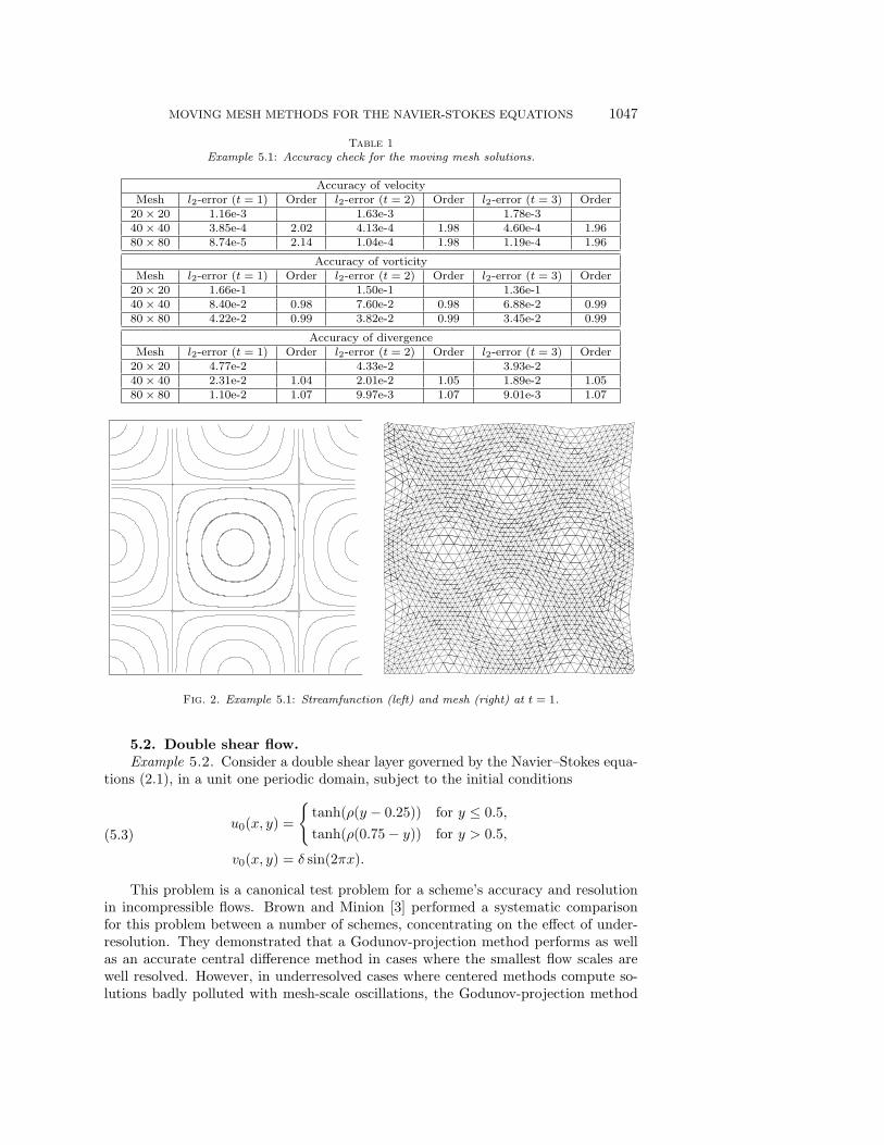
It is noted that the exact solution (5.2) is time separable, and as a result themoving mesh is time independent. Namely, the initial uniform mesh will be movedto a nonuniform one at t = 0, which will remain almost the same at the later time.In Figure 2, the streamline and the moving mesh are plotted at t = 1. It is seen thatthis mesh is different with the initial uniform mesh.


Table 1

Example 5.1: Accuracy check for the moving mesh solutions.

Accuracy of velocityMesh l2-error (t = 1) Order l2-error (t = 2) Order l2-error (t = 3) Order

20 × 20 1.16e-3 1.63e-3 1.78e-340 × 40 3.85e-4 2.02 4.13e-4 1.98 4.60e-4 1.9680 × 80 8.74e-5 2.14 1.04e-4 1.98 1.19e-4 1.96

Accuracy of vorticityMesh l2-error (t = 1) Order l2-error (t = 2) Order l2-error (t = 3) Order

20 × 20 1.66e-1 1.50e-1 1.36e-140 × 40 8.40e-2 0.98 7.60e-2 0.98 6.88e-2 0.9980 × 80 4.22e-2 0.99 3.82e-2 0.99 3.45e-2 0.99

Accuracy of divergenceMesh l2-error (t = 1) Order l2-error (t = 2) Order l2-error (t = 3) Order

20 × 20 4.77e-2 4.33e-2 3.93e-240 × 40 2.31e-2 1.04 2.01e-2 1.05 1.89e-2 1.0580 × 80 1.10e-2 1.07 9.97e-3 1.07 9.01e-3 1.07

Fig. 2. Example 5.1: Streamfunction (left) and mesh (right) at t = 1.

5.2. Double shear flow.Example 5.2. Consider a double shear layer governed by the Navier–Stokes equa-

tions (2.1), in a unit one periodic domain, subject to the initial conditions

u0(x, y) =

tanh(ρ(y − 0.25)) for y ≤ 0.5,

tanh(ρ(0.75 − y)) for y > 0.5,

v0(x, y) = δ sin(2πx).

(5.3)

This problem is a canonical test problem for a scheme’s accuracy and resolutionin incompressible flows. Brown and Minion [3] performed a systematic comparisonfor this problem between a number of schemes, concentrating on the effect of under-resolution. They demonstrated that a Godunov-projection method performs as wellas an accurate central difference method in cases where the smallest flow scales arewell resolved. However, in underresolved cases where centered methods compute so-lutions badly polluted with mesh-scale oscillations, the Godunov-projection method


sometimes gives smooth, apparently physical solutions. It is found in [3] that theseunderresolved solutions, although convergent when the grid is refined, contain spuri-ous nonphysical vortices that are artifacts of the underresolution. It seems necessarythat powerful numerical methods have to be used to resolve the smallest flow scales,which can be done by increasing the accuracy order of the numerical method (see,e.g., [11, 24]) or by using an adaptive grid method. The goal of adaptive grid methodsis to resolve small flow scale by clustering more grid points in the smallest scale areas.

(a) (b)

(c) (d)

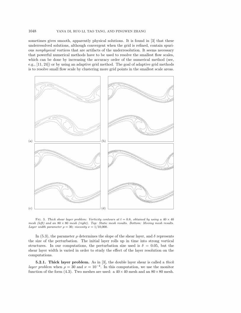
Fig. 3. Thick shear layer problem: Vorticity contours at t = 0.8, obtained by using a 40 × 40mesh (left) and an 80 × 80 mesh (right). Top: Static mesh results. Bottom: Moving mesh results.Layer width parameter ρ = 30; viscosity ν = 1/10,000.

In (5.3), the parameter ρ determines the slope of the shear layer, and δ representsthe size of the perturbation. The initial layer rolls up in time into strong vorticalstructures. In our computations, the perturbation size used is δ = 0.05, but theshear layer width is varied in order to study the effect of the layer resolution on thecomputations.

5.2.1. Thick layer problem. As in [3], the double layer shear is called a thicklayer problem when ρ = 30 and ν = 10−4. In this computation, we use the monitorfunction of the form (4.3). Two meshes are used: a 40×40 mesh and an 80×80 mesh.


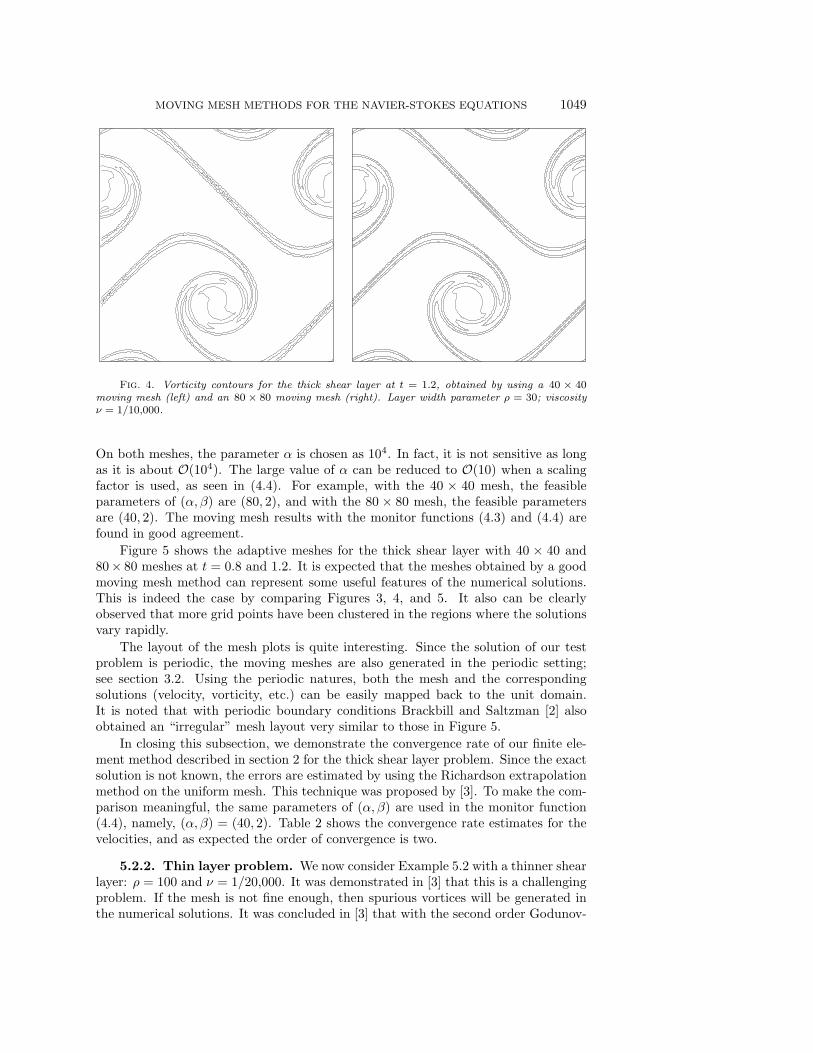
Fig. 4. Vorticity contours for the thick shear layer at t = 1.2, obtained by using a 40 × 40moving mesh (left) and an 80 × 80 moving mesh (right). Layer width parameter ρ = 30; viscosityν = 1/10,000.

On both meshes, the parameter α is chosen as 104. In fact, it is not sensitive as longas it is about O(104). The large value of α can be reduced to O(10) when a scalingfactor is used, as seen in (4.4). For example, with the 40 × 40 mesh, the feasibleparameters of (α, β) are (80, 2), and with the 80 × 80 mesh, the feasible parametersare (40, 2). The moving mesh results with the monitor functions (4.3) and (4.4) arefound in good agreement.

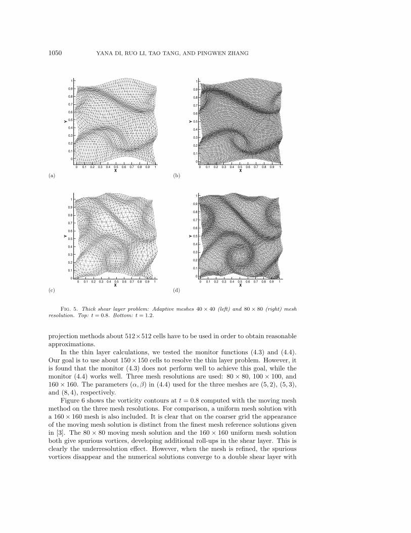
Figure 5 shows the adaptive meshes for the thick shear layer with 40 × 40 and80× 80 meshes at t = 0.8 and 1.2. It is expected that the meshes obtained by a goodmoving mesh method can represent some useful features of the numerical solutions.This is indeed the case by comparing Figures 3, 4, and 5. It also can be clearlyobserved that more grid points have been clustered in the regions where the solutionsvary rapidly.

The layout of the mesh plots is quite interesting. Since the solution of our testproblem is periodic, the moving meshes are also generated in the periodic setting;see section 3.2. Using the periodic natures, both the mesh and the correspondingsolutions (velocity, vorticity, etc.) can be easily mapped back to the unit domain.It is noted that with periodic boundary conditions Brackbill and Saltzman [2] alsoobtained an “irregular” mesh layout very similar to those in Figure 5.

In closing this subsection, we demonstrate the convergence rate of our finite ele-ment method described in section 2 for the thick shear layer problem. Since the exactsolution is not known, the errors are estimated by using the Richardson extrapolationmethod on the uniform mesh. This technique was proposed by [3]. To make the com-parison meaningful, the same parameters of (α, β) are used in the monitor function(4.4), namely, (α, β) = (40, 2). Table 2 shows the convergence rate estimates for thevelocities, and as expected the order of convergence is two.

5.2.2. Thin layer problem. We now consider Example 5.2 with a thinner shearlayer: ρ = 100 and ν = 1/20,000. It was demonstrated in [3] that this is a challengingproblem. If the mesh is not fine enough, then spurious vortices will be generated inthe numerical solutions. It was concluded in [3] that with the second order Godunov-


(a)X

Y

0 0.1 0.2 0.3 0.4 0.5 0.6 0.7 0.8 0.9 1

0

0.1

0.2

0.3

0.4

0.5

0.6

0.7

0.8

0.9

1

(b)X

Y

0 0.1 0.2 0.3 0.4 0.5 0.6 0.7 0.8 0.9 1

0

0.1

0.2

0.3

0.4

0.5

0.6

0.7

0.8

0.9

1

(c)X

Y

0 0.1 0.2 0.3 0.4 0.5 0.6 0.7 0.8 0.9 10

0.1

0.2

0.3

0.4

0.5

0.6

0.7

0.8

0.9

1

(d)X

Y

0 0.1 0.2 0.3 0.4 0.5 0.6 0.7 0.8 0.9 1

0

0.1

0.2

0.3

0.4

0.5

0.6

0.7

0.8

0.9

1

Fig. 5. Thick shear layer problem: Adaptive meshes 40 × 40 (left) and 80 × 80 (right) meshresolution. Top: t = 0.8. Bottom: t = 1.2.

projection methods about 512×512 cells have to be used in order to obtain reasonableapproximations.

In the thin layer calculations, we tested the monitor functions (4.3) and (4.4).Our goal is to use about 150×150 cells to resolve the thin layer problem. However, itis found that the monitor (4.3) does not perform well to achieve this goal, while themonitor (4.4) works well. Three mesh resolutions are used: 80 × 80, 100 × 100, and160 × 160. The parameters (α, β) in (4.4) used for the three meshes are (5, 2), (5, 3),and (8, 4), respectively.

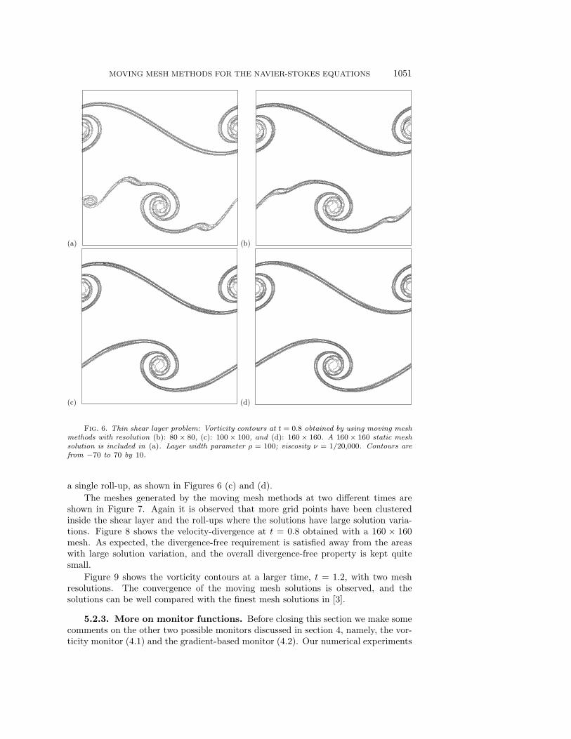
Figure 6 shows the vorticity contours at t = 0.8 computed with the moving meshmethod on the three mesh resolutions. For comparison, a uniform mesh solution witha 160× 160 mesh is also included. It is clear that on the coarser grid the appearanceof the moving mesh solution is distinct from the finest mesh reference solutions givenin [3]. The 80 × 80 moving mesh solution and the 160 × 160 uniform mesh solutionboth give spurious vortices, developing additional roll-ups in the shear layer. This isclearly the underresolution effect. However, when the mesh is refined, the spuriousvortices disappear and the numerical solutions converge to a double shear layer with


(a) (b)

(c) (d)

Fig. 6. Thin shear layer problem: Vorticity contours at t = 0.8 obtained by using moving meshmethods with resolution (b): 80 × 80, (c): 100 × 100, and (d): 160 × 160. A 160 × 160 static meshsolution is included in (a). Layer width parameter ρ = 100; viscosity ν = 1/20,000. Contours arefrom −70 to 70 by 10.

a single roll-up, as shown in Figures 6 (c) and (d).

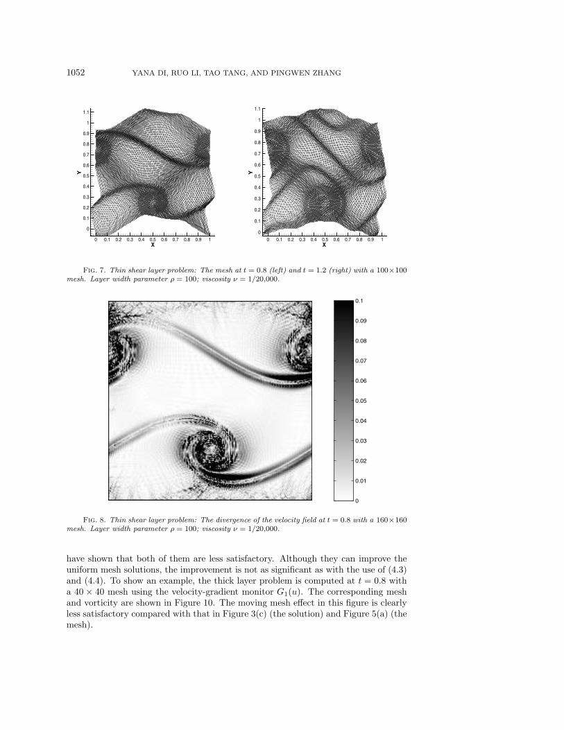
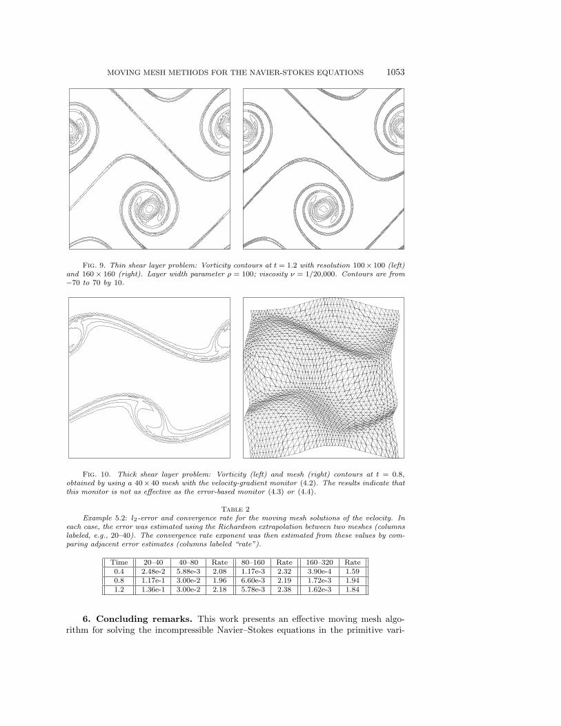
The meshes generated by the moving mesh methods at two different times areshown in Figure 7. Again it is observed that more grid points have been clusteredinside the shear layer and the roll-ups where the solutions have large solution varia-tions. Figure 8 shows the velocity-divergence at t = 0.8 obtained with a 160 × 160mesh. As expected, the divergence-free requirement is satisfied away from the areaswith large solution variation, and the overall divergence-free property is kept quitesmall.

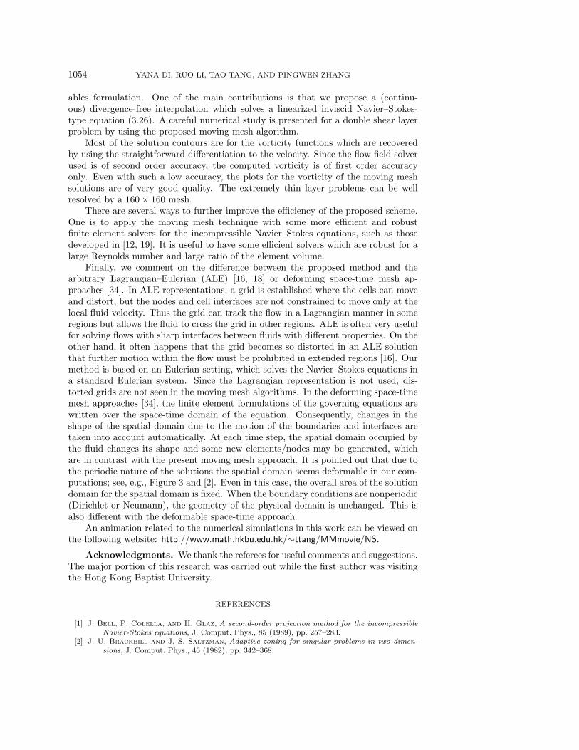
Figure 9 shows the vorticity contours at a larger time, t = 1.2, with two meshresolutions. The convergence of the moving mesh solutions is observed, and thesolutions can be well compared with the finest mesh solutions in [3].

5.2.3. More on monitor functions. Before closing this section we make somecomments on the other two possible monitors discussed in section 4, namely, the vor-ticity monitor (4.1) and the gradient-based monitor (4.2). Our numerical experiments


X

Y

0 0.1 0.2 0.3 0.4 0.5 0.6 0.7 0.8 0.9 1

0

0.1

0.2

0.3

0.4

0.5

0.6

0.7

0.8

0.9

1

1.1

XY

0 0.1 0.2 0.3 0.4 0.5 0.6 0.7 0.8 0.9 10

0.1

0.2

0.3

0.4

0.5

0.6

0.7

0.8

0.9

1

1.1

Fig. 7. Thin shear layer problem: The mesh at t = 0.8 (left) and t = 1.2 (right) with a 100×100mesh. Layer width parameter ρ = 100; viscosity ν = 1/20,000.

0.1

0.09

0.08

0.07

0.06

0.05

0.04

0.03

0.02

0.01

0

Fig. 8. Thin shear layer problem: The divergence of the velocity field at t = 0.8 with a 160×160mesh. Layer width parameter ρ = 100; viscosity ν = 1/20,000.

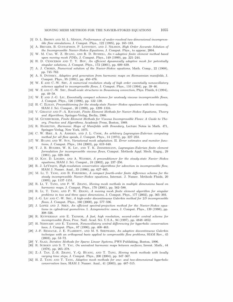
have shown that both of them are less satisfactory. Although they can improve theuniform mesh solutions, the improvement is not as significant as with the use of (4.3)and (4.4). To show an example, the thick layer problem is computed at t = 0.8 witha 40 × 40 mesh using the velocity-gradient monitor G1(u). The corresponding meshand vorticity are shown in Figure 10. The moving mesh effect in this figure is clearlyless satisfactory compared with that in Figure 3(c) (the solution) and Figure 5(a) (themesh).


Fig. 9. Thin shear layer problem: Vorticity contours at t = 1.2 with resolution 100× 100 (left)and 160 × 160 (right). Layer width parameter ρ = 100; viscosity ν = 1/20,000. Contours are from−70 to 70 by 10.

Fig. 10. Thick shear layer problem: Vorticity (left) and mesh (right) contours at t = 0.8,obtained by using a 40× 40 mesh with the velocity-gradient monitor (4.2). The results indicate thatthis monitor is not as effective as the error-based monitor (4.3) or (4.4).

Table 2

Example 5.2: l2-error and convergence rate for the moving mesh solutions of the velocity. Ineach case, the error was estimated using the Richardson extrapolation between two meshes (columnslabeled, e.g., 20–40). The convergence rate exponent was then estimated from these values by com-paring adjacent error estimates (columns labeled “rate”).

Time 20–40 40–80 Rate 80–160 Rate 160–320 Rate0.4 2.48e-2 5.88e-3 2.08 1.17e-3 2.32 3.90e-4 1.590.8 1.17e-1 3.00e-2 1.96 6.60e-3 2.19 1.72e-3 1.941.2 1.36e-1 3.00e-2 2.18 5.78e-3 2.38 1.62e-3 1.84

6. Concluding remarks. This work presents an effective moving mesh algo-rithm for solving the incompressible Navier–Stokes equations in the primitive vari-


ables formulation. One of the main contributions is that we propose a (continu-ous) divergence-free interpolation which solves a linearized inviscid Navier–Stokes-type equation (3.26). A careful numerical study is presented for a double shear layerproblem by using the proposed moving mesh algorithm.

Most of the solution contours are for the vorticity functions which are recoveredby using the straightforward differentiation to the velocity. Since the flow field solverused is of second order accuracy, the computed vorticity is of first order accuracyonly. Even with such a low accuracy, the plots for the vorticity of the moving meshsolutions are of very good quality. The extremely thin layer problems can be wellresolved by a 160 × 160 mesh.

There are several ways to further improve the efficiency of the proposed scheme.One is to apply the moving mesh technique with some more efficient and robustfinite element solvers for the incompressible Navier–Stokes equations, such as thosedeveloped in [12, 19]. It is useful to have some efficient solvers which are robust for alarge Reynolds number and large ratio of the element volume.

Finally, we comment on the difference between the proposed method and thearbitrary Lagrangian–Eulerian (ALE) [16, 18] or deforming space-time mesh ap-proaches [34]. In ALE representations, a grid is established where the cells can moveand distort, but the nodes and cell interfaces are not constrained to move only at thelocal fluid velocity. Thus the grid can track the flow in a Lagrangian manner in someregions but allows the fluid to cross the grid in other regions. ALE is often very usefulfor solving flows with sharp interfaces between fluids with different properties. On theother hand, it often happens that the grid becomes so distorted in an ALE solutionthat further motion within the flow must be prohibited in extended regions [16]. Ourmethod is based on an Eulerian setting, which solves the Navier–Stokes equations ina standard Eulerian system. Since the Lagrangian representation is not used, dis-torted grids are not seen in the moving mesh algorithms. In the deforming space-timemesh approaches [34], the finite element formulations of the governing equations arewritten over the space-time domain of the equation. Consequently, changes in theshape of the spatial domain due to the motion of the boundaries and interfaces aretaken into account automatically. At each time step, the spatial domain occupied bythe fluid changes its shape and some new elements/nodes may be generated, whichare in contrast with the present moving mesh approach. It is pointed out that due tothe periodic nature of the solutions the spatial domain seems deformable in our com-putations; see, e.g., Figure 3 and [2]. Even in this case, the overall area of the solutiondomain for the spatial domain is fixed. When the boundary conditions are nonperiodic(Dirichlet or Neumann), the geometry of the physical domain is unchanged. This isalso different with the deformable space-time approach.

An animation related to the numerical simulations in this work can be viewed onthe following website: http://www.math.hkbu.edu.hk/∼ttang/MMmovie/NS.

Acknowledgments. We thank the referees for useful comments and suggestions.The major portion of this research was carried out while the first author was visitingthe Hong Kong Baptist University.

REFERENCES

[1] J. Bell, P. Colella, and H. Glaz, A second-order projection method for the incompressibleNavier-Stokes equations, J. Comput. Phys., 85 (1989), pp. 257–283.

[2] J. U. Brackbill and J. S. Saltzman, Adaptive zoning for singular problems in two dimen-sions, J. Comput. Phys., 46 (1982), pp. 342–368.


[3] D. L. Brown and M. L. Minion, Performance of under-resolved two-dimensional incompress-ible flow simulations, J. Comput. Phys., 122 (1995), pp. 165–183.

[4] A. Bruger, B. Gustafsson, P. Lotstedt, and J. Nilsson, High Order Accurate Solution ofthe Incompressible Navier-Stokes Equations, J. Comput. Phys., to appear, 2004.

[5] W. M. Cao, W. Z. Huang, and R. D. Russell, An r-adaptive finite element method basedupon moving mesh PDEs, J. Comput. Phys., 149 (1999), pp. 221–244.

[6] H. D. Ceniceros and T. Y. Hou, An efficient dynamically adaptive mesh for potentiallysingular solutions, J. Comput. Phys., 172 (2001), pp. 609–639.

[7] A. J. Chorin, Numerical solution of the Navier-Stokes equations, Math. Comp., 22 (1968),pp. 745–762.

[8] A. S. Dvinsky, Adaptive grid generation from harmonic maps on Riemannian manifolds, J.Comput. Phys., 95 (1991), pp. 450–476.

[9] W. E and C.-W. Shu, A numerical resolution study of high order essentially nonoscillatoryschemes applied to incompressible flows, J. Comput. Phys., 110 (1994), pp. 39–46.

[10] W. E and C.-W. Shu, Small-scale structures in Boussinesq convection, Phys. Fluids, 6 (1994),pp. 49–58.

[11] W. E and J.-G. Liu, Essentially compact schemes for unsteady viscous incompressible flows,J. Comput. Phys., 126 (1996), pp. 122–138.

[12] H. C. Elman, Preconditioning for the steady-state Navier–Stokes equations with low viscosity,SIAM J. Sci. Comput., 20 (1999), pp. 1299–1316.

[13] V. Girault and P.-A. Raviart, Finite Element Methods for Navier-Stokes Equations, Theoryand Algorithms, Springer-Verlag, Berlin, 1986.

[14] M. Gunzburger, Finite Element Methods for Viscous Incompressible Flows: A Guide to The-ory, Practice and Algorithms, Academic Press, Boston, 1989.

[15] R. Hamilton, Harmonic Maps of Manifolds with Boundary, Lecture Notes in Math. 471,Springer-Verlag, New York, 1975.

[16] C. W. Hirt, A. A. Amsden, and J. L. Cook, An arbitrary Lagrangian-Eulerian computingmethod for all flow speeds, J. Comput. Phys., 14 (1974), pp. 227–253.

[17] W. Huang and W. Sun, Variational mesh adaptation. II. Error estimates and monitor func-tions, J. Comput. Phys., 184 (2003), pp. 619–648.

[18] T. J. R. Hughes, W. K. Liu, and T. K. Zimmermann, Lagrangian-Eulerian finite elementformulation for incompressible viscous flows, Comput. Methods Appl. Mech. Engrg., 29(1981), pp. 329–349.

[19] D. Kay, D. Loghin, and A. Wathen, A preconditioner for the steady-state Navier–Stokesequations, SIAM J. Sci. Comput., 24 (2002), pp. 237–256.

[20] R. J. LeVeque, High-resolution conservative algorithms for advection in incompressible flow,SIAM J. Numer. Anal., 33 (1996), pp. 627–665.

[21] M. Li, T. Tang, and B. Fornberg, A compact fourth-order finite difference scheme for thesteady incompressible Navier-Stokes equations, Internat. J. Numer. Methods Fluids, 20(1995), pp. 1137–1151.

[22] R. Li, T. Tang, and P. W. Zhang, Moving mesh methods in multiple dimensions based onharmonic maps, J. Comput. Phys., 170 (2001), pp. 562–588.

[23] R. Li, T. Tang, and P. W. Zhang, A moving mesh finite element algorithm for singularproblems in two and three space dimensions, J. Comput. Phys., 177 (2002), pp. 365–393.

[24] J.-G. Liu and C.-W. Shu, A high-order discontinuous Galerkin method for 2D incompressibleflows, J. Comput. Phys., 160 (2000), pp. 577–596.

[25] J. Lopez and J. Shen, An efficient spectral-projection method for the Navier-Stokes equa-tions in cylindrical geometries. I. Axisymmetric cases, J. Comput. Phys., 139 (1998), pp.308–326.

[26] R. Kupferman and E. Tadmor, A fast, high resolution, second-order central scheme forincompressible flows, Proc. Natl. Acad. Sci. U.S.A., 94 (1997), pp. 4848–4852.

[27] H. Nessyahu and E. Tadmor, Nonoscillatory central differencing for hyperbolic conservationlaws, J. Comput. Phys., 87 (1990), pp. 408–463.

[28] J.-F. Remacle, J. E. Flaherty, and M. S. Shephard, An adaptive discontinuous Galerkintechnique with an orthogonal basis applied to compressible flow problems, SIAM Rev., 45(2003), pp. 53–72.

[29] Y. Saad, Iterative Methods for Sparse Linear Systems, PWS Publishing, Boston, 1996.[30] R. Schoen and S. T. Yau, On univalent harmonic maps between surfaces, Invent. Math., 44

(1978), pp. 265–278.[31] Z.-J. Tan, Z.-R. Zhang, Y.-Q. Huang, and T. Tang, Moving mesh methods with locally

varying time steps, J. Comput. Phys., 200 (2004), pp. 347–367.[32] H. Z. Tang and T. Tang, Adaptive mesh methods for one- and two-dimensional hyperbolic

conservation laws, SIAM J. Numer. Anal., 41 (2003), pp. 487–515.


[33] H. Z. Tang, T. Tang, and P. W. Zhang, An adaptive mesh redistribution method for nonlinearHamilton-Jacobi equations in two- and three-dimensions, J. Comput. Phys., 188 (2003),pp. 543–572.

[34] T. E. Tezduyar, M. Behr, and J. Liou, A new strategy for finite element computations in-volving moving boundaries and interfaces—the deforming-spatial-domain/space-time pro-cedure. I. The concept and the preliminary tests, Comput. Methods Appl. Mech. Engrg.,94 (1992), pp. 339–351.

[35] H. A. van der Vorst, Bi-CGSTAB: A fast and smoothly converging variant of Bi-CG forthe solution of nonsymmetric linear systems, SIAM J. Sci. Statist. Comput., 13 (1992),pp. 631–644.

[36] A. Winslow, Numerical solution of the quasilinear Poisson equation in a nonuniform trianglemesh, J. Comput. Phys., 1 (1967), pp. 149–172.

moving mesh finite element methods for the incompressible navier–stokes...

Documents