mox–report no. 49/2013 fast simulations in matlab for scientific

MOX–Report No. 49/2013

Fast simulations in Matlab for Scientific Computing

Micheletti, S.

MOX, Dipartimento di Matematica “F. Brioschi”Politecnico di Milano, Via Bonardi 9 - 20133 Milano (Italy)

[email protected] http://mox.polimi.it


Stefano Micheletti

14 ottobre 2013

♯ MOX– Modellistica e Calcolo ScientificoDipartimento di Matematica “F. Brioschi”

Politecnico di MilanoPiazza L. da Vinci 32, 20133 Milano, Italy

[email protected]

Sommario

We show how the numerical simulation of typical problems found inScientific Computing can be run efficiently even under the serial Matlabenvironment. This is made possible by a strong employment of vectorizationand sparse matrix manipulation. Numerical examples based on FEMs on2D unstructured triangular grids assess the flexibility and efficiency of thesimulation tool, both on simple elliptic problems as well as on the steadyand unsteady incompressible Navier-Stokes equations. Any type of finiteelements, and 1D and 2D quadrature rules can be easily accommodatedwithin our framework. Emphasis is focused on vectorization programmingand sparse matrix storage and operations, which allow one to obtain veryefficient programs which run in a few minutes on a common notebook.

Keywords: Finite Element Method, Navier-Stokes equations, Programminglanguages

AMS: 68N15, 35Q30, 65N30, 65M60

1

1 Introduction

It is commonly believed that fast numerical simulations of partial differentialequations under the Matlab environment is beyond reach. However, thanks tothe employment of a suitable programming paradigm, we want to show thatthis objective is actually achievable, even on standard notebooks. In particu-lar, we aim at providing the user with a simple and short open-box Matlabimplementation of FEMs on 2D triangular meshes. An early attempt in thisdirection was proposed in [1]. However, we improve on [1] in three respects: 1)efficiency; 2) room for finite elements other than P1; 3) employment of arbitraryquadrature rules. In contrast to [1], we will not deal with the approximationson quadrilateral elements. Actually, once our philosophy has been understood,simple modifications of the proposed codes allow the user to also tackle suchelements. Moreover, the extension to the 3D case is straightforward, once thesuitable geometric data structures are available.

Our main effort has been devoted to the employment, as far as possible, ofvectorized operations. As a matter of fact, the assembly of the stiffness matrix istypically based on the standard loop-over-the-elements (see, e.g., [1, 12, 13, 16]):each triangle of the mesh is processed in turn; the local matrix and right-handside are computed and then assembled into the global matrix and load vector,respectively, exploiting the local-to-global numbering of the degrees of freedom.However, as it stands, this is the actual bottleneck of the whole procedure: thelarger the number of degrees of freedom, the longer the relative time it takesto execute, until the overall computation cost is swamped with the assemblyphase. To overcome this strong limitation, we move from the implementationof the stiffness matrix included in the functions assema and pdeasmc of thepdetool in Matlab [14].1 There, the assembly of the stiffness matrix associatedwith the bilinear form

∫Ω c(x)∇u · ∇v dx, deriving from an elliptic problem, is

carried out. This is performed very efficiently, thanks to the employment ofthe command sparse. On the other hand, this works only for P1 FEM andusing the midpoint quadrature rule. Inspired by this assembly paradigm, wehave extended this philosophy to other differential problems, type of FEMs, andquadrature rules.

The layout of the paper is organized as follows. We start by introducing thedata structure required for describing the mesh in Sect. 2. Here, we employ aso-called minimum data structure, i.e., sufficient for characterizing completelythe lowest order FEM space, i.e., of piecewise linear and continuous functions.This data structure can be then enriched according to the higher order FEMat hand. To illustrate our paradigm on a model problem, the Poisson problemcompleted with Dirichlet boundary conditions is described in Sect. 3 along withthe associated weak and discrete weak formulations, which lay the basis for thesuccessive FEM approximation. In particular, we consider the simple case of

1We are referring to the release 7.9.0.529 (R2009b)

2

Fast simulations in Matlab for Scientific Computing 3

piecewise liner and continuous FEMs and we approximate the integrals involvedin the load vector by the midpoint quadrature rule. Then we extend this basisapproach to the case of a diffusion-reaction problem in Sect. 4. Here we considergeneral mixed (Dirichlet and Neumann) boundary conditions and we incorporatethe use of quadrature rules for both triangles and edges. In Sect. 5, we addressthe discretization of the incompressible Navier-Stokes equations. In particular,we deal with some benchmark problems which aim at computing the drag and liftcoefficients around a cylinder placed in a rectangular channel. These quantitiesinvolve boundary integrals around the cylinder. Instead of directly computingthese integrals, we resort to a “trick” which is sometimes exploited in the finiteelement community. This relies on the weak form of the discretized Navier-Stokes equations and allows one to obtain more accurate results than the directcomputation. The validation on the benchmarks is carried out in Sect. 6. Finally,some conclusions and future developments are gathered in Sect. 7.

2 A minimum data structure

Given an open and bounded polygonal domain Ω ⊂ R2 with boundary ∂Ω, we

denote by Th = K a conformal mesh of Ω = Ω ∪ ∂Ω consisting of trianglesK’s. We want to provide the minimum data structure required for the laterFEM implementation. We take inspiration from the Partial Differential EquationToolbox pde in Matlab. Let us denote by Np, Nt, and Ne the number of vertexes,triangles and boundary edges, respectively, of the actual mesh. Then the toolboxcharacterizes any mesh by the three arrays p,t and e, with dimensions 2 × Np,4× Nt and 7× Ne, respectively. The full description of all of the entries of thesearrays is not required next. Instead, let us just focus on the main ones, whichconstitute the minimum data structure, i.e., sufficient for the description of thepiecewise linear FEMs.The entries

1. p(1:2,i) provide the two coordinates of the i-th vertex, xi, of the mesh;

2. t(1:3,k) yield the global numbering of the three vertexes of the k-thtriangle, in a counterclockwise fashion;

3. e(1:2,j) return the global numbering of the two vertexes of the j-thboundary edge; e(5,j) furnishes the labeling of the portion of the domainboundary containing the j-th boundary edge.

We notice that when these structures are generated by Matlab, e.g., through thecommand initmesh, there is no guarantee that the local ordering of the boun-dary nodes in the array e be counterclockwise. For later use, a post-processingof these nodes may thus be required, and we henceforth assume that this hasbeen carried out. The labeling of the boundary portions of the domain may beuseful for assigning different boundary conditions, e.g., of Dirichlet or Neumann


1

3

7

9

4

1

2

4

3

1

2

5

3

98

11

10612

13

52

4

6

8

5

10

11

12

7

Figura 1: Example of a mesh and numbering of the geometrical entities:boundary portions (blue), vertexes (black) and elements (red).

type, etc. Figure 1 provides an example of a simple mesh comprising 5 boundaryportions (blue), 12 vertexes (black), 13 elements (red), and 9 boundary edges.The reduced data structures t and e are given by

t =

3 1 6 8 1 2 11 7 5 9 4 2 11

12 12 1 1 8 11 12 2 2 2 7 9 9

10 3 3 6 2 1 1 8 7 5 8 11 12

e =

8 7 4 6 5 3 10 12 9

4 5 7 8 9 6 3 10 12

3 5 5 3 4 1 1 2 4

Notice that whereas the ordering of the boundary edges may not be geometricallyconsecutive, the local numbering of the two local nodes of each edge is yetcounterclockwise. Furthermore, for later use, we designate by NΩ and N∂Ω theset of indices, according to their global numbering, of the internal and boundarynodes, respectively.

3 The Poisson model problem

To illustrate our approach, let us start from the model Poisson problem:

−∆u = f in Ω,

u = gD on ∂Ω,(1)

where ∆ is the Laplacian operator, and f, gD are given functions, which wesuppose to be both defined in Ω. With a view to the FEM approximation to


problem (1), we recall its weak formulation. Find u ∈ H10 (Ω) + gD such that

∫

Ω∇u · ∇v dx =

∫

Ωfv dx ∀v ∈ H1

0 (Ω), (2)

where H10 (Ω) is the subspace of the Sobolev space H1(Ω), consisting of functions

that together with their first weak derivatives are Lebesgue integrable, whichhave zero trace on the boundary ([17]), and H1

0 (Ω)+gD = v ∈ H1(Ω) : v−gD ∈H1

0 (Ω). The FEM approximation to (2) is obtained in a straightforward way,after introducing the FEM space V r

h = vh ∈ C0(Ω) : vh|K ∈ Pr(K),∀K ∈ Th,where Pr(K) is the space of polynomials of maximum degree r over K. We thenlet V r

h,0 = V rh ∩H1

0(Ω). Thus the discrete formulation reads: find uh ∈ V rh,0+gD,h

such that ∫

Ω∇uh · ∇vh dx =

∫

Ωfvh dx ∀vh ∈ V r

h,0, (3)

with gD,h ∈ V rh a suitable approximation to gD. It is well known that (3) is

equivalent to an algebraic linear system, say AU = F , where A is the so-calledstiffness matrix, F the load vector, and U collects the degrees of freedom of theFEM space ([7]). To fix ideas, we choose piecewise linear FEMs, i.e., we pickr = 1. In this case, the degrees of freedom are the nodal values, uh(xi), of theFEM function uh at the internal vertexes of the mesh, i.e., those not belongingto the domain boundary. Thus it is possible to expand the discrete solution as

uh(x) =∑

j∈NΩ

uh(xj)φj(x) + gD,h(x), with gD,h(x) =∑

j∈N∂Ω

gD(xj)φj(x),

where φj are the hat basis functions, and gD,h is the FEM function thatinterpolates gD at the boundary nodes. We recall that the hat functions satisfythe conditions

span φiNh

i=1 = V 1h,0; φi(xj) = δij i, j = 1, . . . , Nh,

where xiNh

i=1 denotes the set of the internal vertexes of the mesh, Nh beingthe number of the internal vertexes, while δij is the Kronecker symbol. Thenthe entries, Ai,j, of the stiffness matrix and, Fi, of the load vector are given, fori, j = 1, . . . , Nh, by

Ai,j =

∫

Ω∇φj · ∇φi dx, Fi =

∫

Ωfφi dx−

∑

j∈N∂Ω

gD(xj)

∫

Ω∇φj · ∇φi dx. (4)

In the next example, we pick the data f and gD such that the exact solutionis u = sin(π(x + 1)/2) sin(π(y + 1)/2) on Ω = (−1, 1)2. The following algori-thm gathers the Matlab implementation of the assembling and solution of theresulting algebraic system.


Algorithm 1 1 Np = size(p,2);

2 nD = union(e(1,:),e(2,:));

3 % matrix and vector allocation

4 A = sparse(Np,Np);

5 F = sparse(Np,1);

6 u = sparse(Np,1);

7 % area of triangles and derivatives of the shape functions

8 [ar,g1x,g1y,g2x,g2y,g3x,g3y] = pdetrg(p,t);

9 % local nodes on triangles and centre of mass of triangles

10 n1 = t(1,:);

11 n2 = t(2,:);

12 n3 = t(3,:);

13 xb = (p(1,n1) + p(1,n2) + p(1,n3))/3;

14 yb = (p(2,n1) + p(2,n2) + p(2,n3))/3;

15 % source term and Dirichlet data

16 f = @(x,y) pi^2/2*sin(pi*(x+1)/2).*sin(pi*(y+1)/2);

17 gD = @(x,y) 0*x;

18 % entries of the stiffness matrix

19 a12 = (g1x.*g2x + g1y.*g2y).*ar;

20 a23 = (g2x.*g3x + g2y.*g3y).*ar;

21 a31 = (g3x.*g1x + g3y.*g1y).*ar;

22 % assembling of the stiffness matrix

23 A = A + sparse(n1,n2,a12,Np,Np);



26 A = A + A’;

27 A = A + sparse(n1,n1,-(a12+a31),Np,Np);



30 % assembling of the right-hand side

31 fb = f(xb,yb).*ar/3;

32 F = F + sparse(n1,1,fb,Np,1);



35 % evalutation of the Dirichlet data on the boundary nodes

36 uD = gD(p(1,nD),p(2,nD))’;

37 % construction of the unknown nodes

38 unk = setdiff(1:Np,nD);

39 % elimination of the Dirichlet nodes

40 A = A(unk,:);

41 F = F(unk) - A(:,nD)*uD;

42 A = A(:,unk);

43 % solution of the linear system

44 s = A\F;


45 u(unk) = s;

46 u(nD) = uD;

Some comments are in order.

1. The variable nD at line 2 collects the Dirichlet nodes (in this case the wholeof the boundary nodes);

2. the stiffness matrix, and the load and unknown vectors are allocated atlines 4-6 via the command sparse;

3. the Matlab function pdetrg at line 8 returns the row vector ar containingthe area of all the elements, and the row vectors of the partial derivativeswith respect to x (g1x, g2x, g3x) and to y (g1y, g2y, g3y), of the localbasis functions, according to the local numbering implicitly defined by thearray t. For example, g1x(k) yields the (constant) derivative ∂φ/∂x ofthe basis function associated with the 1st local node of triangle k;

4. the global numbering of the vertexes is computed at lines 10-12, e.g., n1is the row vector of dimension Nt containing the global vertexes that arefirst local nodes of the triangles;

5. the coordinates of the center of mass of all the triangles are computed atlines 13-14;

6. the data f and gD are defined through anonymous functions at lines 16-17;

7. at lines 19-21 the entries of the stiffness matrix are computed, each as arow vector of dimension Nt. For example, a12(k) provides the 1− 2 entrydefined by

a12(k) =

∫

K

∇φ1 · ∇φ2 dx = ∇φ1 · ∇φ2|K|,

where K is the triangle with numbering k, |K| is the area of K, and theintegral can be computed exactly since the integrand is a constant. Thefunctions φ1, φ2 are the two basis functions associated with the local nodes1 and 2 of K, respectively;

8. the assembling of the global stiffness matrix is performed at lines 23-29 viathe command sparse. In particular, sparse(n1,n2,a12,Np,Np) builds asparse matrix of dimension Np×Np and assigns the values a12 to the entriesidentified by the row index n1 and column index n2, i.e., A(n1(k), n2(k)) =a12(k), for k = 1, . . . , Nt. Notice also that the symmetric structure of thematrix, as well as that the row sum is zero are exploited at lines 26 and27-29, respectively;


9. In an analogous fashion, the assembling of the load vector is carried outat lines 31-34. In particular, the first integral involved in the definition ofF in (4) is approximated by the midpoint quadrature rule, i.e.,

F(k) =

∫

K

fφi dx =1

3f(xb(k), yb(k)) |K|,

with (xb(k), yb(k)) the coordinates of the center of mass of K, where eachbasis function attains the value 1/3, and i is here understood to be a localindex ranging in the set 1, 2, 3;

10. The variables uD at line 36 and unk at line 38 define the Dirichlet boun-dary conditions (evaluated in correspondence with the nodes nD) and theunknown vector, respectively. In particular, unk is a column vector whosedimension is given by the cardinality of the internal vertexes. The functionsetdiff performs the set difference between two sets.

11. At lines 40-42 the elimination of the Dirichlet nodes is carried out. Inpractice this amounts to i) discarding the rows in A associated with theboundary nodes, ii) moving the columns corresponding to the Dirichletnodes to the right-hand side, after multiplication by uD;

12. the algebraic system is solved at line 44 via the built-in sparse directsolver, while the assembling of the complete solution vector, including bothinternal and boundary values, is accomplished at the last lines 45-46.

In order to assess the performance of the above algorithm, we have carriedout a test. Namely, we have solved (3), with the same data as above, for se-ven different mesh sizes, repeating each computation ten times. The overallperformance is measured by the average time (over the ten runs) required tocomplete Algorithm 1 for each of the seven cases. The meshes have been ob-tained starting from an initial unstructured grid generated by the command[p,e,t] = initmesh(’squareg’,’hmax’,0.4) (with the function initmesh ofthe pdetool), which is then successively uniformly refined by the command[p,e,t] = refinemesh(’squareg’,p,e,t). This yields meshes characterizedby an average mesh size, h, taking the values 0.2 · 2i−6

i=0 (and is faster thanusing initmesh directly). To measure time, the pair of Matlab functions tic,

toc have been used throughout. The computations have been carried out on anotebook with an Intel R© CoreTM 2 Duo Processor P8600 @ 2.40 GHz, and 4GB RAM. Figure 2 shows the average time, T , in seconds (black ∗), as a function(in log-log scale) of the dimension, S, of the stiffness matrix (after eliminatingthe Dirichlet nodes). The slope of the estimated fit (blue line) is 1.45, showinga superlinear dependence of time on size. To get a feeling about the CPU time,notice that, for a size S on the order of 4 · 104, which is usually considered quitelarge for this problem (in 2D), it takes less than 2 seconds two completely run theprogram. For comparison purposes, the average time, Tl, required by the whole


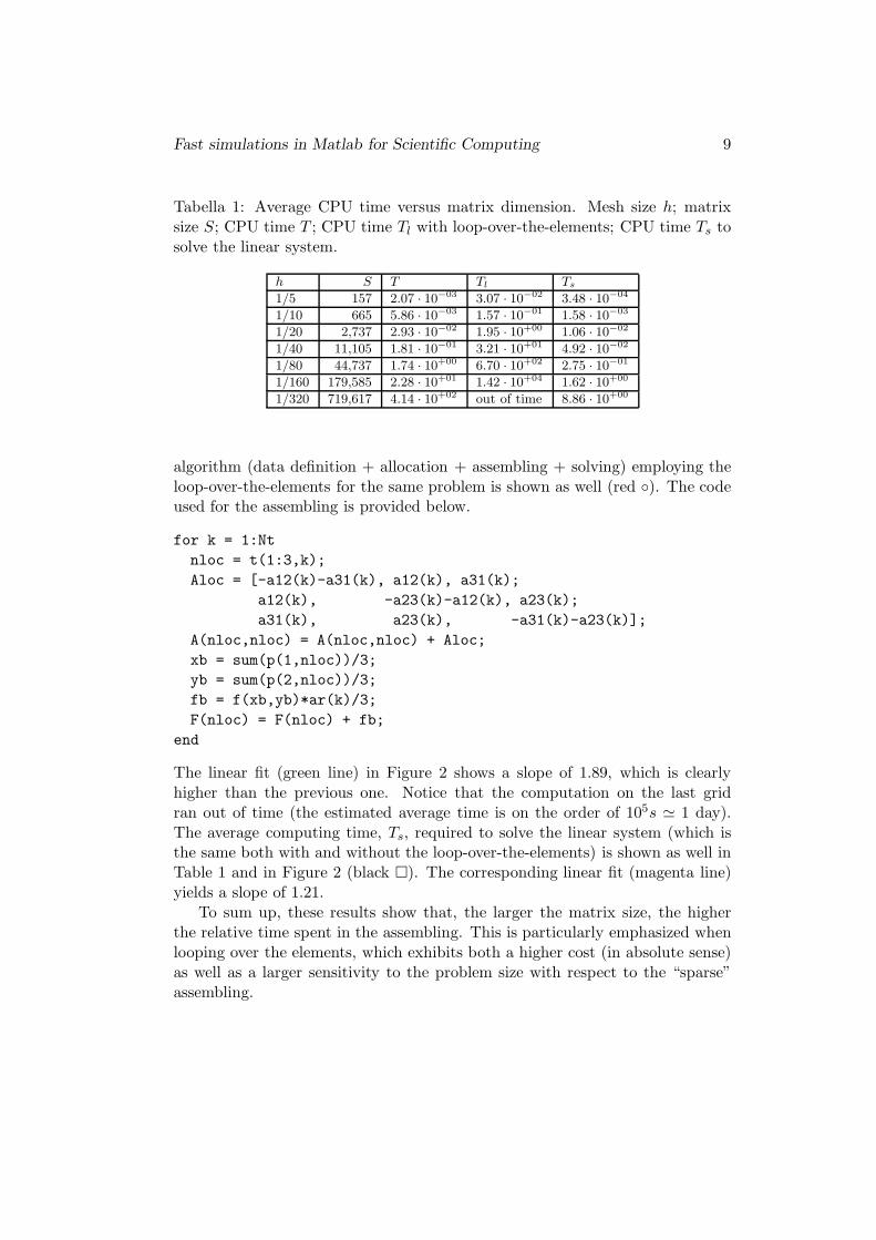
Tabella 1: Average CPU time versus matrix dimension. Mesh size h; matrixsize S; CPU time T ; CPU time Tl with loop-over-the-elements; CPU time Ts tosolve the linear system.

h S T Tl Ts

1/5 157 2.07 · 10−03 3.07 · 10−02 3.48 · 10−04

1/10 665 5.86 · 10−03 1.57 · 10−01 1.58 · 10−03

1/20 2,737 2.93 · 10−02 1.95 · 10+00 1.06 · 10−02

1/40 11,105 1.81 · 10−01 3.21 · 10+01 4.92 · 10−02

1/80 44,737 1.74 · 10+00 6.70 · 10+02 2.75 · 10−01

1/160 179,585 2.28 · 10+01 1.42 · 10+04 1.62 · 10+00

1/320 719,617 4.14 · 10+02 out of time 8.86 · 10+00

algorithm (data definition + allocation + assembling + solving) employing theloop-over-the-elements for the same problem is shown as well (red ). The codeused for the assembling is provided below.

for k = 1:Nt

nloc = t(1:3,k);

Aloc = [-a12(k)-a31(k), a12(k), a31(k);

a12(k), -a23(k)-a12(k), a23(k);

a31(k), a23(k), -a31(k)-a23(k)];

A(nloc,nloc) = A(nloc,nloc) + Aloc;

xb = sum(p(1,nloc))/3;

yb = sum(p(2,nloc))/3;

fb = f(xb,yb)*ar(k)/3;

F(nloc) = F(nloc) + fb;

end

The linear fit (green line) in Figure 2 shows a slope of 1.89, which is clearlyhigher than the previous one. Notice that the computation on the last gridran out of time (the estimated average time is on the order of 105s ≃ 1 day).The average computing time, Ts, required to solve the linear system (which isthe same both with and without the loop-over-the-elements) is shown as well inTable 1 and in Figure 2 (black ). The corresponding linear fit (magenta line)yields a slope of 1.21.

To sum up, these results show that, the larger the matrix size, the higherthe relative time spent in the assembling. This is particularly emphasized whenlooping over the elements, which exhibits both a higher cost (in absolute sense)as well as a larger sensitivity to the problem size with respect to the “sparse”assembling.


102

103

104

105

106

10−4

10−2

100

102

104

106

Figura 2: Average CPU time versus matrix dimension. Black (∗): actual values;blue solid line: linear regression; red (): actual values; green solid line: linearregression (with loop-over-the-elements); black (): actual values; magenta solidline: linear regression (linear system solve).

4 The diffusion-reaction problem

We now deal with the management of quadrature formulas and, for this purpose,we move to an extension of the model Poisson problem, i.e., to the diffusion-reaction problem

−∇ · (µ∇u) + σ u = f in Ω,u = gD on ∂ΓD,

µ∂u

∂n= gN on ∂ΓN ,

(5)

where ΓD ∪ ΓN = ∂Ω with ΓD ∩ ΓN = ∅, gN ∈ C0(ΓN ) is a given function, and∂/∂n designates the outward normal derivative. The functions µ ∈ C0(Ω), withµ ≥ µ0 > 0, and σ ∈ C0(Ω) with σ ≥ 0, represent the diffusion and reactioncoefficient, respectively. As in the previous section, f ∈ C0(Ω) is the source term,while gD ∈ C0(ΓD) is the Dirichlet datum. Although the regularity requirementsfor all of these functions can be relaxed, here we enforce the continuity becauseof the use of quadrature formulas. With a view to the FEM approximation toproblem (5), we recall its weak formulation. Find u ∈ H1

ΓD(Ω) + gD such that

∫

Ωµ∇u · ∇v dx +

∫

Ωσ u v dx =

∫

Ωfv dx +

∫

ΓN

gN v ds ∀v ∈ H1ΓD

(Ω), (6)

where H1ΓD

(Ω) + gD = v ∈ H1(Ω) : v − gD = 0 on ΓD, with H1ΓD

(Ω) = v ∈

H1(Ω) : v = 0 on ΓD. To obtain the FEM approximation to (6), we define the


FEM space V rh,ΓD

= V rh ∩ H1

ΓD(Ω). Thus the discrete formulation reads: find

uh ∈ V rh,ΓD

+ gD,h such that

∫

Ωµ∇uh ·∇vh dx+

∫

Ωσ uh vh dx =

∫

Ωfvh dx+

∫

ΓN

gN vh ds ∀vh ∈ V rh,ΓD

, (7)

with gD,h ∈ V rh a suitable approximation to gD. As in the case of the Poisson

model problem, (7) is equivalent to an algebraic linear system, say AU = F ,where A is still called stiffness matrix, F the load vector, and U collects thedegrees of freedom of the FEM space. For example, with piecewise linear FEMs,i.e., r = 1, the degrees of freedom are the nodal values of the FEM function uh

at the internal vertexes of the mesh and at the nodes belonging to ΓN . Let thetotal number of these vertexes be Nh. Moreover, it holds

uh(x) =∑

j∈NΩ∪NΓN

uh(xj)φj(x) + gD,h(x), with gD,h(x) =∑

j∈NΓD

gD(xj)φj(x),

where φi are the hat basis functions, gD,h is the FEM function that interpolatesgD at the Dirichlet boundary nodes, and we have partitioned the set N∂Ω =NΓN

∪NΓD, with NΓN

∩NΓD= ∅, into the two sets of indices, according to their

global numbering, of the Neumann, NΓN, and Dirichlet, NΓD

nodes, respectively.Then the entries, Ai,j , of the stiffness matrix and, Fi, of the load vector are given,for i, j = 1, . . . , Nh, by

Ai,j =

∫

Ωµ∇φj · ∇φi dx +

∫

Ωσ φj φi dx, (8)

Fi =

∫

Ωfφi dx +

∫

ΓN

gN φi ds−∑

j∈NΓD

gD(xj)

∫

Ωµ∇φj · ∇φi dx.

Notice that now, for general functions µ, σ, f, gN , the corresponding integrals in(8) are no longer exactly computable. Thus it is necessary to resort to somequadrature formulas. These exploit the relations

∫

Ω(·) dx =

∑

K∈Th

∫

K

(·) dx and

∫

ΓN

(·) ds =∑

e∈ΓN

∫

e

(·) ds,

so that we are led to approximate integrals on triangles and edges. In particular,in the first case we employ the Dunavant-type formulas developed by J. Burkardtand downloadable from [4] (see also [5, 18]), while for the second case we use theGauss-Legendre formulas developed by G. von Winckel and available throughthe Matlab Central [22]. We recall that, in general, the quadrature formulas fora dummy function v on a triangle K, and on an edge e read

∫

K

v(x) dx ≃

NKq∑

i=1

wKi v(xK

i ) and

∫

e

v(s) ds ≃

Neq∑

i=1

wei v(s

ei ),


where xKi , w

Ki

NKq

i=1 and sei , w

ei

Neq

i=1 define the pair of NKq and N e

q nodes andweights, for K and e, respectively. Proceeding according to the standard prac-tice in the FEM community, the use of a quadrature rule, either one- or two-dimensional, is carried out by resorting to the so-called reference element. Inparticular, in the two-dimensional case, a reference element, say K, is chosen asthe right-angled triangle with vertexes in (0,0), (1,0), and (0,1). Then any othertriangle, K ∈ Th, can be defined via an affine mapping, TK : K → K, such that

x = TK(x) = MK x + ~tK , (9)

where MK ∈ R2×2 is the (constant) Jacobian of the transformation, and ~tK ∈ R

2

is a shift. If we denote by (xKi , y

Ki )3

i=1, the coordinates of the three vertexesof K (ordered counterclockwise), then it holds

MK =

[xK

2 − xK1 xK

3 − xK1

yK2 − yK

1 yK3 − yK

1

]and ~tK = [xK

1 , yK1 ]T , (10)

so that the vertexes (0,0), (1,0), and (0,1) of K are mapped into (xK1 , y

K1 ),

(xK2 , y

K2 ), and (xK

2 , yK2 ), respectively. The employment of the reference map

facilitates the implementation of the quadrature rule since the nodes and theweights can be defined once and for all on K, and mapped into the actual nodes

and weights on K in a simple way. Let xKi , w

Ki

NKq

i=1 be the node-weight pair

on K, such that

NKq∑

i=1

wKi = 1, then it holds

xKi = TK(xK

i ) and wKi = wK

i |K|. (11)

Moreover, thanks to the differentiation chain rule, it is possible to write thederivative of a function, say v, defined on K in terms of derivatives of thepullback, v, of v by TK , defined on K, where v = v TK , i.e., v(x) = v(TK(x)),∀x ∈ K. In fact, thanks to (9), we have that ∇v = M−T

K ∇v, where

M−TK =

1

2|K|

[yK3 − yK

1 yK1 − yK

2

xK1 − xK

3 xK2 − xK

1

](12)

designates the inverse of the transposed Jacobian in (10). Gathering all thisproperties, it is possible to approximate the contributions to the stiffness matrixand to the load vector. Let us start from the diffusion term:

∫

K

µ∇φj · ∇φi dx =

∫

bK

µM−TK ∇φj ·M

−TK ∇φi |K| dx

≃ |K|

NKq∑

l=1

(wK

l µ(xKl )M−T

K ∇φj(xKl ) ·M−T

K ∇φi(xKl )

). (13)


The reaction contribution is easily dealt with as

∫

K

σ φj φi dx = |K|

∫

bK

σ φj φi dx ≃ |K|

NKq∑

l=1

(wK

l σ(xKl ) φj(x

Kl ) φi(x

Kl )

), (14)

and in an analogous fashion the source term:

∫

K

f φi dx = |K|

∫

bK

f φi dx ≃ |K|

NKq∑

l=1

(wK

l f(xKl ) φi(x

Kl )

). (15)

The remaining term in (8), i.e., the Neumann contribution can be treated usingthe one-dimensional quadrature on the generic edge e ∈ ΓN as:

∫

e

gN φi ds = |e|

∫

be

gN φi ds ≃ |e|

Neq∑

l=1

(we

l gN (sKl ) φi(s

Kl )

), (16)

where now the hatted quantities, say v, are defined through the affine mapTe : e→ e, where e is the reference interval [0, 1], and thus v = v Te.

In the following example we take in (5): Ω = (−1, 1)2, ΓN = (x, y) : x =1 & − 1 < y < 1, ΓD = ∂Ω\ΓN , µ = ex+y, σ = 1 + ex+y, gN = −π

2 sin(π(y +1)/2) ex+y , gD = 0, and we construct f so that u = sin(π(x+1)/2) sin(π(y+1)/2)is the exact solution. Algorithm 2 gathers the Matlab code for computing thenumerical approximation uh in (7) along with the auxiliary function basis atthe bottom.

Algorithm 2

1 Np = size(p,2);

2 Nt = size(t,2);

3 e1 = find(e(5,:)==1); % top

4 e2 = find(e(5,:)==2); % right

5 e3 = find(e(5,:)==3); % bottom

6 e4 = find(e(5,:)==4); % left

7 ne1 = union(e(1,e1),e(2,e1));

8 ne2 = union(e(1,e2),e(2,e2));

9 ne3 = union(e(1,e3),e(2,e3));

10 ne4 = union(e(1,e4),e(2,e4));

11 % number of Neumann edges

12 Nn = length(e2);

13 % Dirichlet nodes

14 nD = unique([ne1,ne3,ne4]);


16 A = sparse(Np,Np);

17 M = sparse(Np,Np);


18 F = sparse(Np,1);

19 u = sparse(Np,1);

20 % area of triangles

21 ar = pdetrg(p,t);

22 % quadrature nodes (2 x nq) and weights (1 x nq) on ref. element

23 % nq = # quadrature nodes, sum(w) = 1

24 [xy, w] = dunavant_rule (3);

25 nq = length(w);

26 % basis functions and derivatives on the ref. element (3 x nq)

27 [phi, phi_x, phi_y] = basis(xy);

28 % local nodes on triangles

29 n1 = t(1,:);

30 n2 = t(2,:);

31 n3 = t(3,:);

32 % coordinates of vertices of triangles

33 x1 = p(1,n1);

34 x2 = p(1,n2);

35 x3 = p(1,n3);

36 y1 = p(2,n1);

37 y2 = p(2,n2);

38 y3 = p(2,n3);

39 % array for the local-to-global nodes

40 loc2glob = t(1:3,:);

41 % local nodes on Neumann edges and edge length

42 nN1 = e(1,e2);

43 nN2 = e(2,e2);

44 lN = sqrt((p(1,nN1)-p(1,nN2)).^2 + (p(2,nN1)-p(2,nN2)).^2);

45 % Gauss-Legendre quadrature (with 3 nodes) on [0,1]

46 [xgl,wgl] = lgwt(3,0,1);

47 xgl = xgl(end:-1:1);

48 % Jacobian of the transformation between ref. element and K

49 % [ x2 - x1, x3 - x1]

50 % [ y2 - y1, y3 - y1]

51 % transponse of the inverse of the Jacobian

52 % [ y3 - y1, y1 - y2]

53 % [ x1 - x3, x2 - x1]/(2*|K|)

54 iMKt11 = (y3 - y1)./(2*ar);

55 iMKt12 = (y1 - y2)./(2*ar);

56 iMKt21 = (x1 - x3)./(2*ar);

57 iMKt22 = (x2 - x1)./(2*ar);

58 % extension of iMKt (nq x Nt)

59 iMKt11q = iMKt11(ones(nq,1),:);





63 % diffusion and reaction coefficients

64 mu = @(x,y) exp(x + y);

65 sigma = @(x,y) 1 + exp(x + y);

66 % source term, Dirichlet and Neumann data

67 f = @(x,y) (pi*exp(x + y).*(2*sin((pi*(x + y))/2) + ...

68 pi*cos((pi*(x + y))/2) + pi*cos((pi*(x - y))/2)))/4 + ...

69 (1 + exp(x + y)).*sin(pi*(x+1)/2).*sin(pi*(y+1)/2);

70 gD = @(x,y) 0*x;

71 gN = @(x,y) -pi/2*sin((pi*(y+1))/2).*exp(x+y);

72 % assembling of lhs and rhs

73 for i = 1:3

74 % extension of the i-th basis function (nq x Nt)

75 phiq = phi (i,:)’; phiq = phiq (:,ones(Nt,1));

76 phi_xq = phi_x(i,:)’; phi_xq = phi_xq(:,ones(Nt,1));

77 phi_yq = phi_y(i,:)’; phi_yq = phi_yq(:,ones(Nt,1));

78 % derivative of the i-th basis function on K

79 Phi_x = iMKt11q.*phi_xq + iMKt12q.*phi_yq;

80 Phi_y = iMKt21q.*phi_xq + iMKt22q.*phi_yq;

81 % quadrature nodes on K (nq x Nt)

82 xq = (1 - xy(1,:) - xy(2,:))’*x1 + xy(1,:)’*x2 + xy(2,:)’*x3;

83 yq = (1 - xy(1,:) - xy(2,:))’*y1 + xy(1,:)’*y2 + xy(2,:)’*y3;

84 % rhs

85 fi = (w*(f(xq,yq).*phiq)).*ar;

86 F = F + sparse(loc2glob(i,:),1,fi,Np,1);

87 for j = 1:3

88 % extension of the j-th basis function (nq x Nt)

89 phjq = phi (j,:)’; phjq = phjq (:,ones(Nt,1));

90 phj_xq = phi_x(j,:)’; phj_xq = phj_xq(:,ones(Nt,1));

91 phj_yq = phi_y(j,:)’; phj_yq = phj_yq(:,ones(Nt,1));

92 % derivative of the j-th basis function on K

93 Phj_x = iMKt11q.*phj_xq + iMKt12q.*phj_yq;

94 Phj_y = iMKt21q.*phj_xq + iMKt22q.*phj_yq;

95 % mass matrix

96 mij = (w*(sigma(xq,yq).*phiq.*phjq)).*ar;

97 M = M + sparse(loc2glob(i,:),loc2glob(j,:),mij,Np,Np);

98 % stiffness matrix

99 aij = (w*(mu(xq,yq).*(Phi_x.*Phj_x + Phi_y.*Phj_y))).*ar;

100 A = A + sparse(loc2glob(i,:),loc2glob(j,:),aij,Np,Np);

101 end

102 end

103 % global stiffness matrix

104 A = A + M;

105 % assembly of the Neumann contribution


106 phi_edge = basis_edge(xgl’);

107 xe = (1 - xgl)*p(1,nN1) + xgl*p(1,nN2);

108 ye = (1 - xgl)*p(2,nN1) + xgl*p(2,nN2);

109 gNe = gN(xe,ye);

110 % extension of the basis function of first node

111 phie = phi_edge(1,:)’; phie = phie(:,ones(Nn,1));

112 fN = (wgl’*(gNe.*phie)).*lN;

113 F = F + sparse(nN1,1,fN,Np,1);

114 % extension of the basis function of second node

115 phie = phi_edge(2,:)’; phie = phie(:,ones(Nn,1));

116 fN = (wgl’*(gNe.*phie)).*lN;

117 F = F + sparse(nN2,1,fN,Np,1);

118 % construction of the unknown nodes

119 unk = setdiff(1:Np,nD);

120 % evalutation of the Dirichlet data on the boundary nodes

121 uD = gD(p(1,nD),p(2,nD))’;

122 % elimination of the Dirichlet nodes

123 A = A(unk,:);

124 A = A(:,unk);

125 F = F(unk) - A(:,nD)*uD;


127 s = A\F;

128 u(unk) = s;

129 u(nD) = uD;

%%%%%%%%%%%%%%%%%%%%%%%%%%%%%%%%%%%%%%%%%%%%%%%%%%%%%%%%%%%%%%

function [phi, phi_x, phi_y] = basis(xy);

Phi = @(x,y) [1 - x - y ; x ; y];

Phi_x = @(x,y) [-ones(size(x)); ones(size(x)) ; zeros(size(x))];

Phi_y = @(x,y) [-ones(size(x)); zeros(size(x)); ones(size(x))];

phi = Phi (xy(1,:),xy(2,:));

phi_x = Phi_x(xy(1,:),xy(2,:));

phi_y = Phi_y(xy(1,:),xy(2,:));

%%%%%%%%%%%%%%%%%%%%%%%%%%%%%%%%%%%%%%%%%%%%%%%%%%%%%%%%%%%%%%

In particular, notice that

1. The four boundary segments defining the domain Ω are numbered cloc-kwise from 1 to 4, starting from the top segment up to the left segment(see lines 3-6). The corresponding nodes are defined at lines 7-10 and theDirichlet nodes at line 14 via the Matlab command unique. Notice thatthe two vertexes at the top-right and bottom-right corners of the domainare Dirichlet nodes. The mesh structures are supposed to be obtained,e.g., through the command [p,e,t] = initmesh(’squareg’,’hmax’,h),where the parameter h controls the maximum edge size of the triangles;


2. the matrix M allocated at line 17 is the mass matrix, i.e., associated onlywith the reaction contribution (14), while A is reserved for the stiffnessmatrix (the diffusion contribution (13), strictly speaking). M is only usedtemporarily; in fact the global matrix is then overwritten to A at line 104;

3. the quadrature nodes on the reference triangle are computed at line 24;notice that the sum of the weights is 1; moreover, the values of the basisfunctions and of their derivatives on the reference element are computedat line 27;

4. at line 40, the array loc2glob whose dimensions are 3 × Nt is formed.It provides the correspondence between local, i.e., 1, 2, 3, and globalnumbering of the nodes. Although it coincides with the mesh array t, thisis only a lucky coincidence due to the choice of the finite elements. Thearray loc2glob will in general set the correspondence between local andglobal degrees of freedom of the finite element space at hand;

5. in the same spirit, at the lines 42-43 the global numbering of the localnodes on the Neumann edges are extracted, along with the length of theseedges at line 44;

6. the nodes and weights of the Gauss-Legendre quadrature formula are com-puted at line 46 and the nodes are successively swapped in ascending orderat line 47;

7. the entries of the inverse of the transposed Jacobian (12) are computedin parallel for each element at the lines 54-57 as arrays of dimension Nt,and are then extended on the quadrature nodes as arrays NK

q ×Nt at lines59-62;

8. the data of the problem are defined at lines 64-71 as anonymous functions;

9. At lines 73-102, the assembling of the mass and stiffness matrices, and ofthe load vector is implemented through two nested loops of size 3 (numberof degrees of freedom of the P1 FEM per element). In particular, we pointout the extension of the basis functions φi at the lines 75-77 and φj at89-91; the construction of the corresponding derivatives on K at 79-80

and 93-94; the computation of contributions due to the source (15) at 85,the diffusion (13) at 99, and the reaction (14) at 96;

10. the contribution due to the Neumann boundary condition is carried out atthe lines 106-117;

11. the program then proceeds by eliminating the rows and columns of theglobal stiffness matrix associated with the Dirichlet nodes, and by takinginto account their effect on the analogously reduced load vector at line125, according to (8);


12. finally, the linear system is solved at line 127 an the complete solution isrecovered in the last two lines;

13. the function basis at the end of the algorithm computes the values ofthe basis functions and of their partial derivatives as functions of the localcoordinates on the reference element.

5 The Navier-Stokes equations

We deal with some test cases that represent typical benchmark problems forthe Navier-Stokes equations ([21]). The objective is to compute some physicalmeaningful quantity, such as the lift and drag coefficients for a cross-section of acylinder in a channel flow, both in steady and unsteady conditions. This allowsus to investigate our algorithmic paradigm on a more challenging situation. Letus consider the conservative form (with respect to the stress rate) of the Navier-Stokes equations for an incompressible fluid, completed with mixed boundaryconditions:

ρ(∂~u∂t

+ (~u · ∇) ~u)−∇ · σ = ~0 in Ω × (0, T ),

∇ · ~u = 0 in Ω × (0, T ),

σ~n = ~0 on ΓN × (0, T ),~u = ~uD on ΓD × (0, T ),~u = ~u0 on Ω at t = 0,

(17)

where the stress rate σ = σ(~u, p) = 2ρν ǫ(~u)−pI depends on the velocity ~u andon the pressure p, while ρ = 1.0 Kg/m3 is the fluid density and ν = 10−3 m2/sis the kinematic viscosity, ǫ(~u) = 1

2

(∇~u+(∇~u)T

)represents the strain rate, and

I denotes the identity tensor. The constant T > 0 represents the final timelevel while ~u0 is a given initial velocity profile. The operator ∇· stands for thedivergence (for both vectors and tensors). As is the case of the Poisson problem(5), ΓD and ΓN are two disjoint portions of the domain boundary.The weak formulation of (17) is: given ~u(0) = ~u0, find (~u(t), p(t)) ∈ (V +~uD)×Q,such that ∀(~v, q) ∈ V ×Q, and t ∈ (0, T ),

0 =

∫

Ωρ

(∂~u∂t

+ (~u · ∇) ~u)· ~v dx +

∫

Ωσ(~u, p) : ǫ(~v) dx −

∫

Ωq∇ · ~udx

=

∫

Ωρ

(∂~u∂t

+ (~u · ∇) ~u)· ~v dx +

∫

Ω2ρνǫ(~u) : ǫ(~v) dx−

∫

Ωp∇ · ~v dx (18)

−

∫

Ωq∇ · ~udx,

where we have introduced the function spaces V = [H1ΓD

(Ω)]2 and Q = L2(Ω),

while the inner product between tensors is denoted by “:”, i.e., σ : ǫ =∑

i,j=1,2

σijǫij .


0 0.5 1 1.5 20

0.2

0.4

0.16

0.15

0.10.15

2.2

Figura 3: Domain Ω for the flow past a cylinder test case.

The benchmarks tests at hand are defined on the rectangular channel Ω,with a width H = 0.41, drilled with a circular hole representing the cross-section of a cylinder and characterized by a slightly asymmetric configuration(see Figure 3). The boundary conditions are prescribed as follows: we takeΓD = Γin ∪ Γcyl ∪ Γwall, where on the inflow section Γin = (x, y) : x = 0 & 0 <y < H, ~u = [vin, 0]

T , with vin = 4Um y (H − y)/H2 the inlet parabolic profile,and Um the peak velocity, while on the remaining rigid walls Γcyl ∪ Γwall, theno-slip constraint ~u = ~0 holds, where Γcyl,Γwall denote the cylinder and the twohorizontal sides, respectively. The Neumann boundary ΓN coincides with theoutlet Γout = (x, y) : x = 2.2 & 0 < y < H and the zero-traction conditionapplies.

The Reynolds number is defined by Re = vinD/ν and is based on the meanvelocity vin over Γin; the cylinder diameter is D = 0.1 m. The chosen physicalquantities

Jdrag = c0

∫

Γcyl

σ(~u, p)~n ·~1‖ ds and Jlift = c0

∫

Γcyl

σ(~u, p)~n ·~1⊥ ds, (19)

represent the so-called drag and lift coefficients, where ~1‖ = [1, 0]T ,~1⊥ = [0, 1]T

are the unit vectors parallel and orthogonal, respectively to the main flow direc-tion (the horizontal one), with c0 = 2/(ρD vin

2). The goal of the benchmarksis to compute these quantities as accurate as possible in an efficient way. Theresults obtained with different approaches by several teams are gathered in [21].Since the purpose of these notes is to present a computational paradigm basedon Matlab, we are not going to push too hard on the computational resour-ces. However, to show that even with a Matlab program run on a notebookfeaturing quite common performances it is still possible to face very challengingproblems, we enhance efficiency by adopting a somewhat original approach thatwe describe below.As already observed, e.g., in [9, 2], the straightforward employment of (19) tocompute the drag and lift coefficients does not yield accurate results, due tothe need of computing numerically first-order derivatives along the cylinder. Amore stable and accurate way is instead obtained by resorting to an interior


rather than a boundary integral. In particular, if we pick any two vector fields,~wdrag, ~wlift : Ω → R

2, associated with the drag and the lift, as suitable extensionsinto Ω of the two unit vectors ~1‖,~1⊥, respectively, i.e., on the boundary

~wdrag =

~1‖ on Γcyl

~0 on ∂Ω\Γcyl

and ~wlift =

~1⊥ on Γcyl

~0 on ∂Ω\Γcyl,(20)

it is possible to replace (19) by the equivalent form

Jdrag = c0

( ∫

Ωρ

(∂~u∂t

+ (~u · ∇) ~u)· ~wdrag dx +

∫

Ωσ(~u, p) : ǫ(~wdrag) dx

),

Jlift = c0

( ∫

Ωρ

(∂~u∂t

+ (~u · ∇) ~u)· ~wlift dx +

∫

Ωσ(~u, p) : ǫ(~wlift) dx

),(21)

where only integrals over Ω are involved. Indeed, from (21), (20) and (17), wehave that

Jdrag = c0

∫

Γcyl

σ(~u, p)~n ·~1‖ ds = c0

∫

Γcyl

σ(~u, p)~n · ~wdrag ds

= c0

∫

∂Ωσ(~u, p)~n · ~wdrag ds = c0

∫

Ω∇ · (σ(~u, p)~wdrag) dx

= c0

(∫

Ω(∇ · σ(~u, p)) · ~wdrag dx +

∫


)

= c0

(∫

Ωρ(∂~u∂t

+ (~u · ∇) ~u)· ~wdrag dx +

∫


),

and analogously for Jlift. Notice that (21) can be interpreted as residuals asso-ciated with the weak formulation (18), where the test function, ~wdrag, ~wlift, donot belong to the space V (due to the nonzero value over Γcyl). In this respect,expressions (21) can be thought of as weak fluxes. These play a key role inDomain Decomposition methods ([20]).On the continuous level, (19) and (21) are thoroughly equivalent (under standardregularity conditions for σ(u, p) and ~wdrag, ~wlift). However, this regularity isdefinitely lost on the discrete level (as long as one does not employ flux conservingFEMs). Nonetheless, after introducing the discrete formulation of (18), we shallemploy the natural discretization to (21) as an accurate evaluation of the dragand lift coefficients.

5.1 Discretization of the Navier-Stokes equations

The discretization of the Navier-Stokes equations with finite elements is addres-sed in, e.g., [6, 11, 15, 19]. The approximation of the weak formulation (18)proceeds in a standard way. As far as the spatial discretization is concerned, weemploy suitable finite element spaces Vh ⊂ V and Qh ⊂ Q, while for the timediscretization we resort to a finite different approximation. Thus, we introduce


the partition tnNT

n=0 consisting of NT + 1 time levels, such that tn+1 = tn + ∆tfor a given constant time step ∆t (such that t0 = 0 and tNT

= T ). The choice ofa uniform mesh is made just for the sake of simplicity. Then, the discretizationof the time derivative ∂~u/∂t consists of the backward Euler method, BE, for thefirst time step (from t0 to t1) and of the second-order Backward DifferentiationFormula, BDF2, for the remaining steps. Both approaches can be given a generalformat, i.e.,

∂~u

∂t(tn+1) ≃

1

∆t

(a1 ~u(tn+1) − a2 ~u(tn) − a3 ~u(tn−1)

), (22)

where a1 = a2 = 1, a3 = 0 (BE), and a1 = 32 , a2 = 2, a3 = −1

2 (BDF2).To deal with the nonlinear convective term (~u · ∇) ~u, we employ the followingextrapolation

[(~u · ∇) ~u](tn+1) ≃ (~u∗(tn+1) · ∇) ~u(tn+1), with ~u∗(tn+1) = b1 ~u(tn) + b2 ~u(tn−1),(23)

where b1 = 1, b2 = 0 (first step) and b1 = 2, b2 = −1 (successive steps). Thuswe use a first-order accurate extrapolation at the first step and a second-ordermethod for the further steps. Overall, the discretizations of the time derivativeand of the nonlinear term ensure a second-order consistency error at the finaltime t = T .

As far as the choice of the finite element spaces, Vh, Qh, it is well known thatany choice will not do. In particular, the so-called discrete inf-sup condition mustbe satisfied in order to obtain a stable discretization ([7]). Neglecting for themoment the boundary conditions, two pairs that are inf-sup stable are providedby the so-called Taylor-Hood element: Vh = (P2)

2 and Qh = P1, and by themini-element (ME): Vh = (P1 ⊕ Pb)

2 and Qh = P1, where Pb denotes the spaceof cubic polynomial bubbles, b, such that, for any K ∈ Th it holds

b ∈ P3(K) ∩H10 (K), 0 ≤ b ≤ 1, b(C) = 1,

where C is the barycenter of K.We are now in a position to state the discrete formulation of the Navier-Stokes

equations. We let ~unh ≃ ~u(tn), pn

h ≃ p(tn), n = 0, 1, . . . , NT . Then given ~u 0h , we

are to find (~un+1h , pn+1

h ) ∈ (Vh +~uD,h)×Qh such that, for n = 0, 1, 2, . . . , NT − 1

∫

Ωρ

( a1

∆t~un+1

h +((b1 ~u

nh + b2 ~u

n−1h ) · ∇

)~un+1

h

)· ~vh dx

+

∫

Ω2ρν ǫ(~un+1

h ) : ǫ(~vh) dx−

∫

Ωpn+1

h ∇ · ~vh dx−

∫

Ωqh ∇ · ~un+1

h dx

=

∫

Ω

ρ

∆t

(a2 ~u

nh + a3 ~u

n−1h

)· ~vh ∀(~vh, qh) ∈ Vh ×Qh, (24)

where ~u 0h , ~uD,h are suitable approximations to ~u0, ~uD, and Vh ⊂ [H1

ΓD(Ω)]2, Qh ⊂

L2(Ω).


In the following test cases, we employ the discrete space ME. Thus the degreesof freedom of the velocity can be chosen as the values taken at the vertexes ofthe mesh belonging to NΩ ∪NΓN

and at the centroids of the elements, while thedegrees of freedom of the pressure are associated with the values attained at allthe vertexes NΩ∪NΓN

∪NΓD. Let us denote the set of the indices associated with

the degrees of freedom of each velocity component as NU , and of the pressure asNP , where it is understood that the first |NΩ ∪ NΓN

| indices of NU correspondto the P1 degrees of freedom (value at vertex), | · | being the cardinality of aset, while the remaining Nt indices are associated with the Pb degrees of freedom(value at centroid), whereas the degrees of freedom of the pressure are all oftype P1. Let us then denote for brevity by NU = |NΩ ∪NΓN

|+ Nt and NP = Np

the cardinalities of the two sets NU and NP , respectively. After introducing thisnotation, problem (24) admits an algebraic counterpart which we now describe.Expand the discrete velocity-pressure pair at an arbitrary time level n as

~unh (x) =

∑

j∈NU

~unh (xj)φj(x) + ~un

D,h(x), with ~unD,h(x) =

∑

j∈NΓD

~unD(xj)φj(x),

pnh(x) =

∑

j∈NP

pnh(xj)ψj(x),

where ~unD,h is a suitable approximation to the exact data ~uD(tn) constructed

only via P1 degrees of freedom, since the bubble functions are zero on the whole∂Ω. Other choices for ~un

D,h are clearly possible but this turns out to be handyin the implementation. The functions φj and ψj collect the basis functionsfor the velocity and the pressure, respectively. For a given time level, n, we nowcollect the degrees of freedom of the velocity in the vector Un ∈ R

2NU , withUn = [Un

1 ,Un2 ]T , where Un

i ∈ RNU gathers the degrees of freedom associated

with the i-th component of the velocity field, for i = 1, 2, and we group thedegrees of freedom of the pressure in the vector Pn ∈ R

NP .Then the algebraic counterpart of (24) reads: given [U0,P0]T ∈ R

2NU+NP ,for n = 0, 1, 2, . . . , NT − 1 find Wn+1 = [Un+1,Pn+1]T ∈ R

2NU+NP such that

AnWn+1 = Fn+1, (25)

where An ∈ R(2NU +NP )×(2NU +NP ) is given by

An =

[ a1

∆tM +A+N(b1U

n + b2Un−1) BT

B 0

], (26)

and the right-hand side Fn+1 ∈ R2NU+NP is

Fn+1 =

[Fn+1

u + 1∆tM(a2U

n + a3Un−1)

Fn+1p

]. (27)


Matrix M ∈ R2NU×2NU is the mass matrix of the velocity, A ∈ R

2NU×2NU is thestiffness matrix associated with the viscous stresses, N(·) ∈ R

2NU×2NU is the ma-trix associated with the advective term, B ∈ R

NP×2NU collects the contributionsof the ”divergence” term; on the right-hand side, Fn+1

u ∈ R2NU and Fn+1

p ∈ RNP

gather the quantities associated with the Dirichlet conditions at time level n+1,and all the contributions of the previous time steps. In more detail, all of thesematrices have the following block structure: M is the symmetric two-by-twoblock diagonal matrix

M =

[Mu 00 Mu

],

with Mu ∈ RNU×NU (and zero blocks of the same size), and

[Mu]i,j =

∫

Ωρφjφi dx, i, j ∈ NU ;

A is the symmetric two-by-two block matrix

A =

[A11 A12

AT12 A22

],

where the four blocks are the RNU×NU matrices, for i, j ∈ NU , given by

[A11]i,j =

∫

Ω2ρν ǫ([φj , 0]

T ) : ǫ([φi, 0]T ) dx =

∫

Ω2ρν

(∂φj

∂x

∂φi

∂x+

1

2

∂φj

∂y

∂φi

∂y

)dx

[A12]i,j =

∫

Ω2ρν ǫ([φj , 0]

T ) : ǫ([0, φi]T ) dx =

∫

Ω2ρν

1

2

∂φj

∂x

∂φi

∂ydx

[A22]i,j =

∫

Ω2ρν ǫ([0, φj ]

T ) : ǫ([0, φi]T ) dx =

∫

Ω2ρν

(∂φj

∂y

∂φi

∂y+

1

2

∂φj

∂x

∂φi

∂x

)dx;

N(~vh), for a dummy discrete velocity field ~vh, is the nonsymmetric two-by-twoadvection matrix

N(~vh) =

[Nu 00 Nu

],

with Nu ∈ RNU×NU (and zero blocks of the same size), and

[Nu]i,j =

∫

Ωρ~vh · ∇φj φi dx, i, j ∈ NU ;

B is the one-by-two block matrix

B = [B1 B2],

with Bi ∈ RNP×NU , for i = 1, 2, and

[B1]i,j = −

∫

Ω

∂φj

∂xψi dx, [B2]i,j = −

∫

Ω

∂φj

∂yψi dx, i ∈ NP , j ∈ NU ;


Fn+1u is given by [Fn+1

u,1 Fn+1u,2 ]T , with Fn+1

u,i ∈ RNU , i = 1, 2, and, for i ∈ NU ,

[Fn+1u,1 ]

i= −

∫

Ωρ

( a1

∆t~un+1

D,h +((b1 ~u

nh + b2 ~u

n−1h ) · ∇

)~un+1

D,h

)· [φi, 0]

T dx

+

∫

Ωǫ(~un+1

D,h ) : ǫ([φi, 0]T ) dx +

∫

Ω

ρ

∆t

(a2 ~u

nh + a3 ~u

n−1h

)· [φi, 0]

T

[Fn+1u,2 ]

i= −

∫

Ωρ

( a1

∆t~un+1

D,h +((b1 ~u

nh + b2 ~u

n−1h ) · ∇

)~un+1

D,h

)· [0, φi]

T dx

+

∫

Ωǫ(~un+1

D,h ) : ǫ([0, φi]T ) dx +

∫

Ω

ρ

∆t

(a2 ~u

nh + a3 ~u

n−1h

)· [0, φi]

T ,

while Fn+1p ∈ R

Np has components

[Fn+1p ]i =

∫

Ωψi∇ · ~un+1

D,h dx, i ∈ NP .

Notice that the matrix An in (26) is time dependent due to the advectioncontribution only.

As for the actual computation of the drag and lift, we adopt the discretecounterpart of (21), replacing the pair (~u, p) with (~uh, ph), approximating thetime derivative with the corresponding finite differences, and using as ~wdrag, ~wlift

the harmonic finite element functions which satisfy (20) obtained as follows. Wefirst construct the harmonic function, Zh ∈ P1 ⊕ Pb, satisfying Zh = 1 on Γcyl

and Zh = 0 on ∂Ω\Γcyl. Then we define ~wdrag = [Zh, 0]T and ~wlift = [0, Zh]T .

On the discrete level, this amounts to computing the quantity

Jdrag = c0[Z 0]T (AnWn+1 − Fn+1) Jlift = c0[0 Z]T (AnWn+1 − Fn+1), (28)

where Z ∈ R2NU collects the degrees of freedom of the function Zh, and the zero

block has dimension NP .

6 The benchmark test cases

We are now ready to present the numerical results on some benchmarks proposedin [21]. For simplicity, here we only focus on the drag and lift coefficients.Other quantities, such as pressure difference, Strouhal number and length ofrecirculation will not be addressed.

6.1 Test case 2D-1

This is a stationary test case, with Um = 0.3, and thus Re = 20. The dragand lift coefficients have to be computed. Table 2 summarizes the results forthis test case, showing the number of elements, Nt, the number of vertexes, Np,the size of the global stiffness matrix, S, the average CPU time, T1, requiredto complete one time step, the values of the drag and lift coefficients, for three


0 0.5 1 1.5 2

0.2

0.4

0.1 0.15 0.2 0.25 0.30.1

0.12

0.14

0.16

0.18

0.2

0.22

0.24

0.26

0.28

Figura 4: First mesh for the test case 2D-1 (left) and zoom in on the cylinder(right).

Tabella 2: Test case 2D-1. Number of elements Nt; number of nodes Np; matrixsize S; average CPU time per time step T1; drag coefficient Jdrag ; lift coefficientJlift.

Nt Np S T1 Jdrag Jlift

3,392 1,788 11,794 0.9 5.5811 · 10+00−2.8478 · 10−03

13,568 6,968 47,334 4.3 5.5799 · 10+00 7.1270 · 10−03

15,560 7,980 54,318 5.1 5.5798 · 10+00 2.3325 · 10−02

different computational meshes. The first mesh (see Figure. 4) exhibits somerefinement around the cylinder. In particular, 32 elements are placed aroundthe cylinder. The second mesh is obtained through a uniform refinement of thefirst one, i.e., each triangle is divided into four similar triangle by joining themid-edges, and thus it has 64 elements attached to the cylinder. The third meshis a uniform mesh characterized by a maximum mesh size of 0.014 throughoutall of the domain. Around the cylinder there are only 24 elements. The number,S, of global unknowns is comparable to the coarsest and medium size meshes ofthe benchmarks reported in [21], which span from 6,562 to 30,775,296. In orderto get the steady state solution, we chose ∆t = 10−2 and T = 8. The values inTable 2 for the drag coefficient are consistent with the range deduced in [21], i.e.,5.5700 ≤ Jdrag ≤ 5.5900. For this test case, the lift coefficient turns out to bethe most critical quantity to compute. Actually, the values in Table 2, althoughnot strictly in the range 1.04 · 10−02 ≤ Jlift ≤ 1.10 · 10−02 suggested in [21], arein any case of the same order as many of the values reported in [21]. Notice alsothat, it takes about 13 minutes (in the best case) and 1 hour (in the worst) forthe program to execute a full sweep over 800 time steps.

6.2 Test case 2D-2

This is an unsteady test case, where Um = 1.5, yielding Re = 100. It is requi-red to compute the drag and lift coefficients as functions of time for one period[t0, t0 + 1/f ] (with f = f(Jlift)), maximum drag coefficient, Jdrag,M , maximumlift coefficient, Jlift,M . The initial data (t = t0) should correspond to the flowstate with Jlift,M . For the simulation, we employed ∆t = 10−2 and T = 8. Ta-


ble 3 shows the maximum value of the drag, Jdrag,M , and lift, Jlift,M coefficientsover the period. The computational work per time step is the same as in the pre-vious test case. The computed values appear to be comparable to the referencevalues in [21], i.e., 3.2200 ≤ Jdrag,M ≤ 3.2400 and 0.9900 ≤ Jlift,M ≤ 1.0100.

Tabella 3: Test case 2D-2. Number of elements Nt; number of nodes Np; matrixsize S; average CPU time per time step T1; maximum drag coefficient Jdrag,M ;maximum lift coefficient Jlift,M .

Nt Np S T1 Jdrag,M Jlift,M

3,392 1,788 11,794 0.9 3.2289 · 10+00 1.0088 · 10+00

13,568 6,968 47,334 4.3 3.2529 · 10+00 1.0385 · 10+00

15,560 7,980 54,318 5.1 3.1065 · 10+00 8.0528 · 10−01

6.3 Test case 2D-3

Tabella 4: Test case 2D-3. Number of elements Nt; number of nodes Np; matrixsize S; average CPU time per time step T1; maximum drag coefficient Jdrag,M ;maximum lift coefficient Jlift,M .

Nt Np S T1 Jdrag,M Jlift,M

3,392 1,788 11,794 0.9 2.9106 · 10+00 5.5318 · 10−01

13,568 6,968 47,334 4.3 2.9370 · 10+00 5.7065 · 10−01

15,560 7,980 54,318 5.1 2.8843 · 10+00 4.3683 · 10−01

This is a time dependent problem, where the inflow condition is vin =4Um y (H − y) sin(πt/8)/H2, with Um = 1.5, and the time interval is 0 ≤ t ≤ 8.This gives a time varying Reynolds number between 0 ≤ Re(t) ≤ 100. Theinitial data (t = 0) are ~u0 = ~0, P = 0. The following quantities should be com-puted: drag and lift coefficients as functions of time for 0 ≤ t ≤ 8, maximumdrag coefficient, Jdrag,M , and maximum lift coefficient, Jlift,M . Although notexplicitly mentioned in [21], the value of vin to be used in the definitions (19)is the value associated with the maximum height of the inflow profile, i.e., att = 4. Table 4 gathers the results for this test case. Again, ∆t = 10−2 andT = 8 were chosen. Also in this case, the computed drag and lift coefficients areconsistent with the reference values in [21], i.e., 2.9300 ≤ Jdrag,M ≤ 2.9700 and0.4700 ≤ Jlift,M ≤ 0.4900.

The full list of the program, for the test case 2D-1, is provided in theAppendix.


7 Conclusions

We have developed a numerical tool for solving problems described by partialdifferential equations. In particular, our tool is based on a simple and short open-box Matlab implementation of FEMs on 2D triangular meshes. Our effort hasbeen mainly devoted to making the program as efficient as possible, in order torun in few seconds or minutes (in case of a steady simulation). The employmentof Matlab is by no means restrictive. Our choice was mainly motivated by thefact that it still represents a very popular interactive environment for numericalcomputation, visualization, and programming. However, simple modificationsallow one to adapt our tool to other high-level interpreted languages, such asGNU Octave [10].

To describe our approach, we have first considered the Poisson problem,completed with both Dirichlet and Neumann boundary conditions, as one of thetypical problems which appear in Scientific Computing. Then we have generali-zed this to the diffusion-reaction problem, where both the diffusion and reactioncoefficients, as well as the boundary data may vary as a function of position,thus requiring the use of suitable quadrature rules. Finally, we have dealt withthe steady and unsteady incompressible Navier-Stokes equations. In all cases,it turns out that low computing times can be really achieved even for the morechallenging problems represented by the Navier-Stokes equations. This was ma-de possible by first adopting a suitable data structure to describe the mesh, andsecondly, by a thorough use of vectorization programming and sparse matrixstorage and operations which is made possible within the Matlab environment.Only 2D configurations have been addressed in this paper. However, we havealready extended all of this techniques to the 3D case, and impressive improve-ments of the computing times can be obtained also in this case. As a possibletask for the future, it would be desirable to develop a tool for easily generatinga data structure suitable to deal with higher-order polynomials, i.e., Pk, withk ≥ 2.

Appendix A

Algorithm 3 1 % physical and geometrical parameters

2 rho = 1;

3 nu = 1e-3;

4 mu = rho*nu;

5 Um = 0.3;

6 H = 0.41;

7 D = 0.1;

8 Ubar = 2*(4*Um*H/2*(H-H/2)/H^2)/3; % mean inflow velocity

9 Re = Ubar*D/nu;

10


11 % data for time discretization

12 dt = 0.01;

13 Tf = 8;

14 time = linspace(0,Tf,Tf/dt+1);

15

16 % load mesh and geometry: p, e, t

17 load cylinder

18

19 % classification of the nodes

20 [ninf,nout,ndir,nunk] = find_nodes(p,e,t);

21

22 % choice of FEM space

23 % ’TH’ = Taylor-Hood (P2/P1)

24 % ’ME’ = Mini-element (P1b/P1)

25 element = ’ME’

26

27 % coefficients of backward Euler

28 a1 = 1; a2 = 1; a3 = 0;

29

30 % extrapolation of convective term: b1*u^n + b2*u^n-1

31 % at first time step: first-order extrapolation

32 b1 = 1; b2 = 0;

33

34 % quadrature nodes (2 x nq) and weights (1 x nq) on ref. triangle

35 % sum(w) = 1

36 [ xy, w ] = dunavant_rule (5);

37 nq = length(w);

38

39 % velocity (phi) and pressure (psi) basis functions

40 % on the reference triangle: nb x nq, nb = # local basis functions

41 [phi, phi_x, phi_y, psi, psi_x, psi_y] = basis(xy,element);

42

43 % number of global dofs for velocity (dofV) and pressure (dofP)

44 % loc2globV: nbV x Nt

45 % loc2globP: nbP x Nt

46 [dofV, dofP, loc2globV, loc2globP] = dofs(p,t,element);

47

48 % area of triangles and number of vertices and elements

49 ar = pdetrg(p,t);

50 Nt = size(t,2);

51 Np = size(p,2);

52

53 nbV = size(phi,1); % # local basis functions for velocity

54 nbP = size(psi,1); % # local basis functions for pressure


55 ZZ = sparse(dofP,dofP);

56 ZP = sparse(dofP,1);

57

58 % initial conditions

59 U = sparse(dofV,1);

60 U1 = sparse(dofV,1); % u^n-1

61 U2 = sparse(dofV,1); % u^n-2

62 V = sparse(dofV,1); % v^n-1

63 V1 = sparse(dofV,1); % v^n-2

64 V2 = sparse(dofV,1);

65 P = sparse(dofP,1);

66

67 % coordinates of local (1, 2 and 3) node of each triangle

68 n1 = t(1,:);

69 n2 = t(2,:);

70 n3 = t(3,:);

71 x1 = p(1,n1);

72 x2 = p(1,n2);

73 x3 = p(1,n3);

74 y1 = p(2,n1);

75 y2 = p(2,n2);

76 y3 = p(2,n3);

77


79 A = sparse(2*dofV+dofP,2*dofV+dofP);

80 F = sparse(2*dofV+dofP,1);

81 M = sparse(dofV,dofV);

82 A11 = sparse(dofV,dofV);



85 B1t = sparse(dofV,dofP);

86 B2t = sparse(dofV,dofP);

87

88 % Jacobian of the mapping from reference element to K

89 % [ x2 - x1, x3 - x1]

90 % [ y2 - y1, y3 - y1]

91 %

92 % inverse of transposed Jacobian

93 % [ y3 - y1, y1 - y2]

94 % [ x1 - x3, x2 - x1]/(2*|K|)

95 iMKt11 = (y3 - y1)./(2*ar);

96 iMKt12 = (y1 - y2)./(2*ar);

97 iMKt21 = (x1 - x3)./(2*ar);

98 iMKt22 = (x2 - x1)./(2*ar);


99 % extension on the quadrature nodes of iMKt





104

105 % lift and drag initialization

106 cD = zeros(length(time),1);

107 cL = zeros(length(time),1);

108

109 for n = 1:(length(time)-1)

110

111 N1 = sparse(dofV,dofV);

112 N2 = sparse(dofV,dofV);

113

114 if n == 1

115

116 for i = 1:nbV

117

118 % extension of the i-th basis function: nq x Nt




122 % derivative of i-th basis function on K



125

126 for j = 1:nbV

127

128 % extension of the j-th basis function: nq x Nt




132

133 % velocity mass matrix

134 mij = rho*(w*(phiq.*phjq)).*ar/dt;

135 M = M + sparse(loc2globV(i,:),loc2globV(j,:),mij,dofV,dofV);

136

137 % derivative of j-th basis function on K



140

141 % viscous strains stiffness matrix

142 a11 = 2*mu*(w*(Phi_x.*Phj_x + Phi_y.*Phj_y/2)).*ar;


143 a12 = 2*mu*(w*(Phi_y.*Phj_x/2)).*ar;

144 a22 = 2*mu*(w*(Phi_y.*Phj_y + Phi_x.*Phj_x/2)).*ar;

145 A11 = A11 + sparse(loc2globV(i,:),loc2globV(j,:),a11,dofV,dofV);



148

149 % convection matrix N(u_h)

150 for l = 1:nbV

151 U1K = U1(loc2globV(l,:))’;


153 V1K = V1(loc2globV(l,:))’;


155 phlq = phi (l,:)’; phlq = phlq (:,ones(Nt,1));

156 nl1 = w*(phiq.*phlq.*Phj_x).*(b1*U1K + b2*U2K).*ar;

157 nl2 = w*(phiq.*phlq.*Phj_y).*(b1*V1K + b2*V2K).*ar;

158 N1 = N1 + sparse(loc2globV(i,:),loc2globV(j,:),nl1,dofV,dofV);


160 end

161

162 end

163

164 for j = 1:nbP

165

166 psjq = psi (j,:)’; psjq = psjq (:,ones(Nt,1));

167 % ‘‘divergence’’ matrix B

168 b1t = -(w*(Phi_x.*psjq)).*ar;

169 b2t = -(w*(Phi_y.*psjq)).*ar;

170 B1t = B1t + sparse(loc2globV(i,:),loc2globP(j,:),b1t,dofV,dofP);

171 B2t = B2t + sparse(loc2globV(i,:),loc2globP(j,:),b2t,dofV,dofP);

172

173 end

174 end

175

176 % auxiliary variable for drag & lift

177 Z = compute_Z(p,e,t,ar,nbV,dofV,dofP,loc2globV,w,phi_x,phi_y);

178

179 else

180

181 for i = 1:nbV

182 % extension of the i-th basis function: nq x Nt




186 % derivative of i-th basis function on K




189

190 for j = 1:nbV

191

192 % extension of the j-th basis function: nq x Nt




196 % derivative of j-th basis function on K



199

200 % advection matrix N(u_h)

201 for l = 1:nbV





206 phlq = phi (l,:)’; phlq = phlq (:,ones(Nt,1));

207 nl1 = w*(phiq.*phlq.*Phj_x).*(b1*U1K + b2*U2K).*ar;

208 nl2 = w*(phiq.*phlq.*Phj_y).*(b1*V1K + b2*V2K).*ar;



211 end

212

213 end

214 end

215 end

216

217 N = rho*(N1 + N2);

218 % global stiffness and load vector

219 A = [a1*M+A11+N, A12 , B1t;

220 A12’ , a1*M+A22+N, B2t;

221 B1t’ , B2t’ , ZZ ];

222

223 F = [M*(a2*U1+a3*U2); M*(a2*V1+a3*V2); ZP];

224

225 % boundary conditions at inflow

226 uinf = assign_inflow(p,ninf,Um,H,time(n+1));

227

228 % global indices of unknowns

229 unk_glob = [nunk,Np+(1:Nt),dofV + [nunk,Np+(1:Nt)],2*dofV+(1:Np)];

230 Aglob = A;


231 Fglob = F;

232 A = A(unk_glob,:);

233 F = F(unk_glob);

234 F = F - A(:,ninf)*uinf;

235 A = A(:,unk_glob);

236


238 numb_unkV = length(nunk) + Nt;

239 uvp = A\F;

240 u = uvp(1:numb_unkV);

241 v = uvp([1:numb_unkV] + numb_unkV);

242 P = uvp(2*numb_unkV+1:end);

243 U([nunk,(1:Nt)+Np]) = u;

244 V([nunk,(1:Nt)+Np]) = v;

245 U(ninf) = uinf;

246

247 % drag & lift computation

248 [cD(n+1), cL(n+1)] = compute_drag_lift(dofV,dofP,Aglob,Fglob,...

U,V,P,Z,rho,Ubar,D);

249

250 % update velocity for next time step

251 U2 = U1;

252 U1 = U;

253 V2 = V1;

254 V1 = V;

255

256 % coefficient of BDF2

257 a1 = 3/2; a2 = 2; a3 = -1/2;

258 % coefficients of second-order extrapolation

259 b1 = 2; b2 = -1;

260

261 end

The auxiliary functions required by this program are gathered below

function [ninf,nout,ndir,nunk] = find_nodes(p,e,t)

% ninf = inflow nodes

% nout = outflow nodes

% ndir = Dirichlet nodes = ninf + walls + cylinder

% nout = unknown nodes = internal + outflow

Np = size(p,2);

% 1 = right


% 2 = top

% 3 = left

% 4 = bottom

% 5-8 = cylinder

e1 = find(e(5,:) == 1);

e2 = find(e(5,:) == 2);

e3 = find(e(5,:) == 3);

e4 = find(e(5,:) == 4);

e5 = find(e(5,:) == 5);

e6 = find(e(5,:) == 6);

e7 = find(e(5,:) == 7);

e8 = find(e(5,:) == 8);

n1 = union(e(1,e1),e(2,e1));

n2 = union(e(1,e2),e(2,e2));

n3 = union(e(1,e3),e(2,e3));

n4 = union(e(1,e4),e(2,e4));

n5 = union(e(1,e5),e(2,e5));

n6 = union(e(1,e6),e(2,e6));

n7 = union(e(1,e7),e(2,e7));

n8 = union(e(1,e8),e(2,e8));

ninf = n3;

nout = setdiff(n1,union(n2,n4));

ndir = unique([n2,n3,n4,n5,n6,n7,n8]);

nunk = setdiff(1:Np,ndir);

%%%%%%%%%%%%%%%%%%%%%%%%%%%%%%%%%%%%%%%%%%%%%%%%%%%%%%%%%%%%%%%%%%%%

function [phi, phi_x, phi_y, psi, psi_x, psi_y] = basis(xy,element);

switch element

case ’TH’

disp(’TH element not yet implemented’)

case ’ME’

Phi = @(x,y) [1 - x - y ; x ; y ; ...

27*(1 - x - y)*x*y];

Phi_x = @(x,y) [-ones(size(x)); ones(size(x)) ; zeros(size(x)); ...

-27*y*(2*x+y-1)];

Phi_y = @(x,y) [-ones(size(x)); zeros(size(x)); ones(size(x)) ; ...


-27*x*(2*y+x-1)];

phi = Phi (xy(1,:),xy(2,:));

phi_x = Phi_x(xy(1,:),xy(2,:));

phi_y = Phi_y(xy(1,:),xy(2,:));

%

psi = phi(1:3,:);

psi_x = phi_x(1:3,:);

psi_y = phi_y(1:3,:);

otherwise

disp(’Unknown method!’)

end

%%%%%%%%%%%%%%%%%%%%%%%%%%%%%%%%%%%%%%%%%%%%%%%%%%%%%%%%%%%%%%%%%%%%

function [dofV, dofP, loc2globV, loc2globP] = dofs(p,t,element);

Np = size(p,2);

Nt = size(t,2);

% Euler’s theorem: Nt + Np = Nl + 1 (where Nl = # all edges)

switch element

case ’TH’

display(’TH element not yet implemented’)

case ’ME’

dofV = Np + Nt;

dofP = Np;

loc2globV = zeros(4,Nt);

loc2globV(1:3,:) = t(1:3,:);

loc2globV(4,:) = Np + [1:Nt];

loc2globP = t(1:3,:);

otherwise

disp(’Unknown method!’)

end

%%%%%%%%%%%%%%%%%%%%%%%%%%%%%%%%%%%%%%%%%%%%%%%%%%%%%%%%%%%%%%%%%%%%

function uinf = assign_inflow(p,ninf,Um,H,t)


y = p(2,ninf)’;

uinf = 4*Um*y.*(H-y)/H^2;

% for test case 2D-3

%uinf = 4*Um*y.*(H-y)*sin(pi*t/8)/H^2;

%%%%%%%%%%%%%%%%%%%%%%%%%%%%%%%%%%%%%%%%%%%%%%%%%%%%%%%%%%%%%%%%%%%%

function Z = compute_Z(p,e,t,ar,nbV,dofV,dofP,loc2globV,wq,phi_x,phi_y)

% computes the auxiliary velocity variable Z:

% -Delta Z = 0 in Omega

% Z = 1 on cylinder

% Z = 0 elsewhere

Np = size(p,2);

Nt = size(t,2);

nq = length(wq);

% 1 = right

% 2 = top

% 3 = left

% 4 = bottom

% 5-8 = cylinder

e1 = find(e(5,:) == 1);

e2 = find(e(5,:) == 2);

e3 = find(e(5,:) == 3);

e4 = find(e(5,:) == 4);

e5 = find(e(5,:) == 5);

e6 = find(e(5,:) == 6);

e7 = find(e(5,:) == 7);

e8 = find(e(5,:) == 8);

n1 = union(e(1,e1),e(2,e1));

n2 = union(e(1,e2),e(2,e2));

n3 = union(e(1,e3),e(2,e3));

n4 = union(e(1,e4),e(2,e4));

n5 = union(e(1,e5),e(2,e5));

n6 = union(e(1,e6),e(2,e6));

n7 = union(e(1,e7),e(2,e7));

n8 = union(e(1,e8),e(2,e8));


ndir1 = unique([n5,n6,n7,n8]);

ndir0 = unique([n1,n2,n3,n4]);

nunk = setdiff(1:Np,[ndir0,ndir1]);

nK1 = t(1,:);

nK2 = t(2,:);

nK3 = t(3,:);

x1 = p(1,nK1);

x2 = p(1,nK2);

x3 = p(1,nK3);

y1 = p(2,nK1);

y2 = p(2,nK2);

y3 = p(2,nK3);

% Jacobian from reference element to K

% [ x2 - x1, x3 - x1]

% [ y2 - y1, y3 - y1]

%

% The transposed inverse Jacobian from reference element to K

% [ y3 - y1, y1 - y2]

% [ x1 - x3, x2 - x1]/(2*|K|)

iMKt11 = (y3 - y1)./(2*ar);

iMKt12 = (y1 - y2)./(2*ar);

iMKt21 = (x1 - x3)./(2*ar);

iMKt22 = (x2 - x1)./(2*ar);

% extension of iMKt

iMKt11q = iMKt11(ones(nq,1),:);




A = sparse(dofV,dofV);

F = sparse(dofV,1);

Z = sparse(dofV,1);

for i = 1:nbV

% extension of the i-th basis function: nq x Nt

phi_xq = phi_x(i,:)’; phi_xq = phi_xq(:,ones(Nt,1));

phi_yq = phi_y(i,:)’; phi_yq = phi_yq(:,ones(Nt,1));

% derivative of i-th basis function on K

Phi_x = iMKt11q.*phi_xq + iMKt12q.*phi_yq;

Phi_y = iMKt21q.*phi_xq + iMKt22q.*phi_yq;


for j = 1:nbV

% extension of the j-th basis function: nq x Nt

phj_xq = phi_x(j,:)’; phj_xq = phj_xq(:,ones(Nt,1));

phj_yq = phi_y(j,:)’; phj_yq = phj_yq(:,ones(Nt,1));

% derivative of j-th basis function on K

Phj_x = iMKt11q.*phj_xq + iMKt12q.*phj_yq;

Phj_y = iMKt21q.*phj_xq + iMKt22q.*phj_yq;

% stiffness matrix of Laplacian

a = (wq*(Phi_x.*Phj_x + Phi_y.*Phj_y)).*ar;

A = A + sparse(loc2globV(i,:),loc2globV(j,:),a,dofV,dofV);

end

end

unk_glob = [nunk,Np+(1:Nt)];

A = A(unk_glob,:);

F = F(unk_glob);

F = F - A(:,ndir1)*ones(length(ndir1),1);

A = A(:,unk_glob);

s = A\F;

Z(ndir1) = 1;

Z(unk_glob) = s;

%%%%%%%%%%%%%%%%%%%%%%%%%%%%%%%%%%%%%%%%%%%%%%%%%%%%%%%%%%%%%%%%%%%%

function [cD, cL] = compute_drag_lift(dofV,dofP,Aglob,Fglob,U,V,P,Z,rho,Ubar,D)

W = sparse(2*dofV+dofP,1);

W(1:dofV) = Z;

drag = W’*(Aglob*[U;V;P]-Fglob);

%

W = sparse(2*dofV+dofP,1);

W((1:dofV)+dofV) = Z;

lift = W’*(Aglob*[U;V;P]-Fglob);

cD = 2*drag/(rho*Ubar^2*D);

cL = 2*lift/(rho*Ubar^2*D);

%%%%%%%%%%%%%%%%%%%%%%%%%%%%%%%%%%%%%%%%%%%%%%%%%%%%%%%%%%%%%%%%%%%%


Riferimenti bibliografici

[1] J. Alberty, C. Carstensen, and S. A. Funken, Remarks around 50lines of Matlab: short finite element implementation, Numerical Algorithms,20 (1999), pp. 117–137.

[2] W. Bangerth and R. Rannacher, Adaptive Finite Element Methods forDifferential Equations, Lectures in Mathematics, ETH Zurich, BirkhauserVerlag, Basel, 2003.

[3] R. Becker, Weighted error estimators for the incompressible Navier-Stokesequations, Rapport de recherche, 3458, INRIA, 1998.

[4] J. Burkardt

http://people.sc.fsu.edu/~jburkardt/m_src/dunavant/dunavant_

html, 2006.

[5] D. Dunavant, High degree efficient symmetrical Gaussian quadrature rulesfor the triangle, Internat. J. Numer. Methods Engrg., 21 (1985), pp. 1129–1148.

[6] H. Elman, D. Silvester, and A. Wathen, Finite Elements and Fa-st Iterative Solvers: with Applications in Incompressible Fluid Dynamics,Oxford University Press, New-York, 2005.

[7] A. Ern and J. L. Guermond, Theory and Practice of Finite Elements,Text in Applied Mathematica Sciences, 159, Springer-Verlag, New-York,2004.

[8] M. B. Giles, M. G. Larson, J. M. Levenstam, and E. Suli, Adaptiveerror control for finite element approximations of the lift and drag coef-ficients in viscous flow, Technical Report, NA-97/06, Oxford UniversityComputing Laboratory, 1997.

[9] M. B. Giles and E. Suli, Adjoint methods for PDEs: a posteriori erroranalysis and postprocessing by duality, Acta Numer., 11 (2002), pp. 145–236.

[10] www.gnu.org/software/octave

[11] P. M. Gresho, and R. L. Sani, Incompressible Flow and the FiniteElement Method, voll. I and II, John Wiley & Sons, 2000.

[12] P. I. Kattan, MATLAB Guide to Finite Elements: An interactiveapproach, Springer-Verlag, Berlin, 2008.

[13] Y. W. Kwon, and H.C. Bang, The Finite Element Method UsingMATLAB, 2nd Edition, CRC Press, 2000.


[14] Partial Differential Equation ToolboxTMUser’s Guide, The MathWorks,Inc., http://www.mathworks.com/access/helpdesk/help/toolbox/

pde/, 2011.

[15] W. Layton Introduction to the Numerical Analysis of Incompressible Vi-scous Flows, Society for Industrial and Applied Mathematics (SIAM),Philadelphia, PA, 2008.

[16] J. Li, and Yi-T. Chen, Computational Partial Differential Equationsusing MATLAB, CRC Press, 2009.

[17] J. L. Lions and E. Magenes, Non-Homogeneous Boundary ValueProblems and Applications, vol. I. Springer-Verlag, Berlin, 1972.

[18] J. Lyness and D. Jespersen, Moderate degree symmetric quadrature rulesfor the triangle, J. Inst. Math. Appl., 15(1) (1975), pp. 19–32.

[19] A. Quarteroni, Numerical Models for Differential Problems, Springer-Verlag Italia, Milan, 2009.

[20] A. Quarteroni and A. Valli, Domain Decomposition Methods forPartial Differential Equations, Numerical Mathematics and ScientificComputation, Clarendon Press, Oxford, 1999.

[21] M. Schaefer and S. Turek, Benchmark computations of laminar flowaround a cylinder, in NNFM 52 “Flow Simulation on High-PerformanceComputers II”, Vieweg, Braunschweig, 1996.

[22] G. von Winckel, Matlab Central,http://www.mathworks.com/matlabcentral/fileexchange/

4540-legendre-gauss-quadrature-weights-and-nodes, 2004.

MOX Technical Reports, last issuesDipartimento di Matematica “F. Brioschi”,

Politecnico di Milano, Via Bonardi 9 - 20133 Milano (Italy)

49/2013 Micheletti, S.


48/2013 Simone Palamara, Christian Vergara, Elena Faggiano, Fabio

Nobile

An effective algorithm for the generation of patient-specific Purkinje

networks in computational electrocardiology

47/2013 Chkifa, A.; Cohen, A.; Migliorati, G.; Nobile, F.; Tempone,

R.

Discrete least squares polynomial approximation with random evalua-

tions - application to parametric and stochastic elliptic PDEs

46/2013 Marron, J.S.; Ramsay, J.O.; Sangalli, L.M.; Srivastava, A.

Statistics of Time Warpings and Phase Variations

45/2013 Sangalli, L.M.; Secchi, P.; Vantini, S.

Analysis of AneuRisk65 data: K-mean Alignment

44/2013 Sangalli, L.M.; Secchi, P.; Vantini, S.

AneuRisk65: a dataset of three-dimensional cerebral vascular geome-

tries

43/2013 Patriarca, M.; Sangalli, L.M.; Secchi, P.; Vantini, S.

Analysis of Spike Train Data: an Application of K-mean Alignment

42/2013 Bernardi, M.; Sangalli, L.M.; Secchi, P.; Vantini, S.

Analysis of Juggling Data: an Application of K-mean Alignment

41/2013 Bernardi, M.; Sangalli, L.M.; Secchi, P.; Vantini, S.

Analysis of Proteomics data: Block K-mean Alignment

40/2013 Pacciarini P.; Rozza G.

Stabilized reduced basis method for parametrized advection-diffusion PDEs

mox–report no. 49/2013 fast simulations in matlab for scientific

Documents