MP-208: Optimal Filtering with Aerospace ApplicationsChapter 1: Introduction

Davi Antonio dos Santos

Department of MechatronicsInstituto Tecnologico de Aeronautica

davists@ita.br

Sao Jose dos Campos, BrazilFebruary 2019

1 / 15

Contents

1 Preliminary Definitions

2 History

3 Aerospace Applications

4 Example

2 / 15

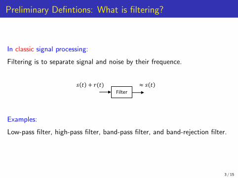
Preliminary Defintions: What is filtering?

In classic signal processing:

Filtering is to separate signal and noise by their frequence.

≈ 𝑠(𝑡) 𝑠(𝑡) + 𝑟(𝑡) Filter

Examples:

Low-pass filter, high-pass filter, band-pass filter, and band-rejection filter.

3 / 15

Preliminary Definitions: What is filtering?

In statistical signal processing:

Filtering is to separate signal from noise by their statistical properties. Weare intereseted in this type of filtering!

≈ 𝑠(𝑡) 𝑠(𝑡) + 𝑟(𝑡) Filter

≈ 𝑠(𝑡) ℎ(𝑠(𝑡), 𝑟(𝑡)) Filter

Examples:

Wiener filter, Kolmogorov filter, Kalman filter, Bucy filter, etc.

4 / 15

Preliminary Definitions: What is filtering?

Three types of state estimation: prediction, filtering, and smoothing:

time

time

time

5 / 15

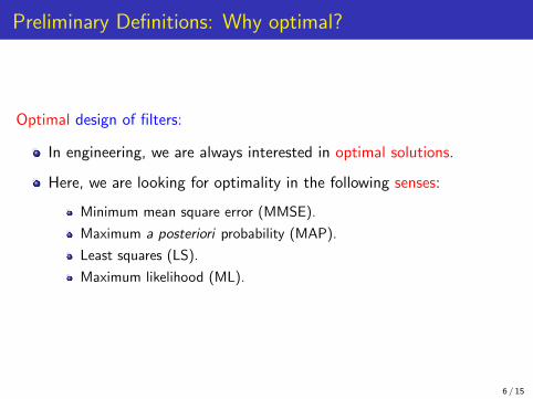
Preliminary Definitions: Why optimal?

Optimal design of filters:

In engineering, we are always interested in optimal solutions.

Here, we are looking for optimality in the following senses:

Minimum mean square error (MMSE).

Maximum a posteriori probability (MAP).

Least squares (LS).

Maximum likelihood (ML).

6 / 15

History

The Optimal Filtering has been constructed in the following sequence:

1795: Johann Carl Friedrich Gauss devised the Least-Squares methodfor estimating the Ceres’ orbit.

1940’s: Wiener/Kolmogorov Filter to separate signal from noise usingthe MMSE criterion. They used a frequecy-domain approach.

1950’s: Attempts to extend Wiener/Kolmogorov filters for non-stationaryand multivariate signals.

1960: Kalman-Bucy Filter was introduced as the new approach totackle and extend the Weiner and Kolmogorov problems for non-stationaryand multivariate signals.

1960-1970: Numerous applications in satellite orbit determination aswell as in attitude determination and navigation of aircrafts, ships,rockets, etc.

7 / 15

History

1960-1970: Optimal Nonlinear Filtering developed from works by Strato-novich (Russia) and consolidated from the works by Kushner (EUA).

1990-: Particle Filters or sequential Monte Carlo methods.

1990-: More approximations of the Kalman filter for nonlinear systems:unscented Kalman filter, cubature Kalman filter, ensemble Kalman fil-ter, etc.

8 / 15

Aerospace Applications

Regarding the dynamic nature of the quantity we want to estimate, we candistinguish between two types of estimation:

Parameter estimation: the parameters are quantities that characterizethe system of interest. Their values are assumed to be constant orsmoothly time-varying.

State estimation: The states are (time-varying) signals that describethe system dynamics.

9 / 15

Aerospace Applications

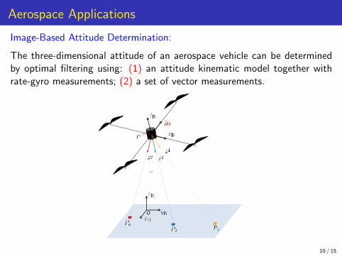
Image-Based Attitude Determination:

The three-dimensional attitude of an aerospace vehicle can be determinedby optimal filtering using: (1) an attitude kinematic model together withrate-gyro measurements; (2) a set of vector measurements.

𝑂

10 / 15

Aerospace Applications

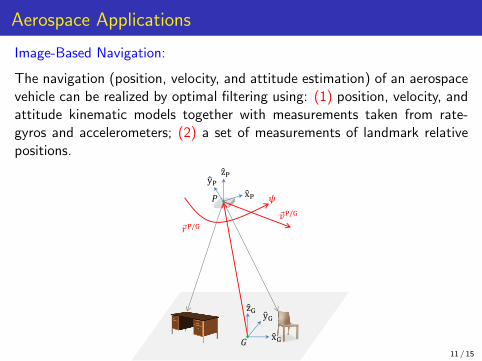
Image-Based Navigation:

The navigation (position, velocity, and attitude estimation) of an aerospacevehicle can be realized by optimal filtering using: (1) position, velocity, andattitude kinematic models together with measurements taken from rate-gyros and accelerometers; (2) a set of measurements of landmark relativepositions.

𝑟 P/G

𝑣 P/G

𝜓

z P y P

x P 𝑃

𝐺

z G

x G

y G

11 / 15

Aerospace Applications

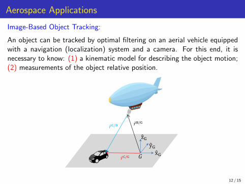
Image-Based Object Tracking:

An object can be tracked by optimal filtering on an aerial vehicle equippedwith a navigation (localization) system and a camera. For this end, it isnecessary to know: (1) a kinematic model for describing the object motion;(2) measurements of the object relative position.

𝑟 C/B

𝐺

z G

x G

y G

𝑟 B/G

𝑟 C/G

12 / 15

Aerospace Applications

In aerospace systems, the most frequent applications of parameter esti-amtion are:

Calibration of navigation sensors.

System identification.

13 / 15

Example

Height and Vertical Velocity Estimation:

Consider an MAV equipped with an ultrasonic sensor for measuring its heighthk at each discrete-time instant k. Assume that the sensor is noise-free anddenote the variable representing its measure at k > 0 by yk .

1 Obtain a dynamic model of the plant in the discrete-time state-spacerepresentation.

2 Design a Luenberger observer, with eigenvalues λ1 = 0.1 and λ2 = 0.1,for estimating the height hk and the vertical velocity hk using themeasurements yk , k > 0.

3 Implement and test the observer using MATLAB script.

14 / 15

References

Bar-Shalom, Y.; Li, X.R.; Kirubarajan, T. Estimation with Applica-tions to Tracking and Navigation. New York: John Wiley & Sons,2001.

Markley, F. L.; Crassidis, J. L. Fundamentals of Spacecraft AttitudeDetermination and Control. Springer, 2014.

Gelb, A. (Ed) Applied Optimal Estimation. Cambridge: MIT Press,1974.

Jazwinski, A. H. Stochastic Processes and Filtering Theory. NewYork: Dover, 2007.

15 / 15