mpi - a stata command for the alkire-foster methodology · 2017-11-06 · // basic mpi command. mpi...
TRANSCRIPT

mpiA Stata command for the Alkire-Foster methodology
Christoph Jindra
OPHI Seminar Series - Michaelmas 2015
9 November 2015
Christoph Jindra (Research Officer) 9 November 2015 1 / 30

OutlineWhat and whyData and indicators for examplesThe syntax
General syntaxMinimal expressionMissing values
OptionsWeightsMultidimensional FGT classRaw and censored headcounts and dimensional breakdownSubgroup analysisSaved resultsDominance approach using graphs
To do listLiteratureChristoph Jindra (Research Officer) 9 November 2015 2 / 30
What and why
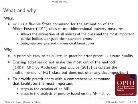
What and whyWhat
I mpi is a flexible Stata command for the estimation of theAlkire-Foster (2011) class of multidimensional poverty measures
I Allows the estimation of all indices of the class and the most importantpartial indices alongside their standard errors
I Subgroup analysis and dimensional breakdownWhy
I In principle easy to calculate, in practice error prone → assure qualityI Existing ado-files do not make the most out of the method
(IMDP_AFI by Abdelkrim and Duclos (2013) calculates themultidimensional FGT class but does not offer any decomposition)
I To provide practitioners with a comprehensive commandthat facilitates the most important
I steps in the creation of an MPII steps in the analysis of poverty based on the AF-method
Christoph Jindra (Research Officer) 9 November 2015 3 / 30
Data and indicators for examples
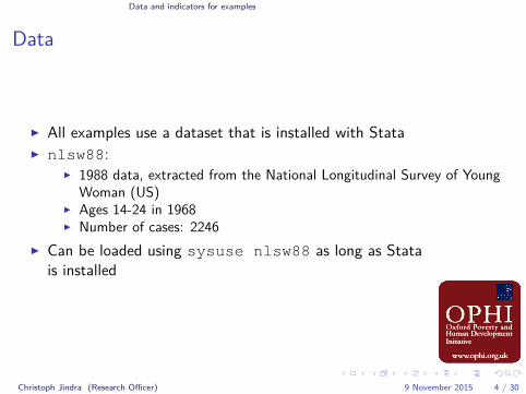
Data
I All examples use a dataset that is installed with StataI nlsw88:
I 1988 data, extracted from the National Longitudinal Survey of YoungWoman (US)
I Ages 14-24 in 1968I Number of cases: 2246
I Can be loaded using sysuse nlsw88 as long as Statais installed
Christoph Jindra (Research Officer) 9 November 2015 4 / 30
Data and indicators for examples
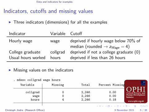
Indicators, cutoffs and missing valuesI Three indicators (dimensions) for all the examples
Indicator Variable CutoffHourly wage wage deprived if hourly wage below 70% of
median (rounded → zWage = 4)College graduate collgrad deprived if not a college graduate (0)Usual hours worked hours deprived if less than 26 hours
I Missing values on the indicators
. mdesc collgrad wage hoursVariable Missing Total Percent Missing
collgrad 0 2,246 0.00wage 0 2,246 0.00
hours 4 2,246 0.18
Christoph Jindra (Research Officer) 9 November 2015 5 / 30
The syntax General syntax
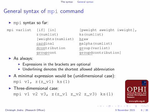
General syntax of mpi command
I mpi syntax so far:mpi varlist [if] [in] [pweight aweight iweight],
z(numlist) ks(numlist)[weights(numlist) hrawcardinal malpha(numlist)dcontribution group(varlist)groupcont groupdcontribution]
I As always:I Expressions in the brackets are optionalI Underlining denotes the shortest allowed abbreviation
I A minimal expression would be (unidimensional case):mpi v1, z(z_v1) ks(1)
I Three-dimensional case:mpi v1 v2 v3, z(z_v1 z_v2 z_v3) ks(1)
Christoph Jindra (Research Officer) 9 November 2015 6 / 30
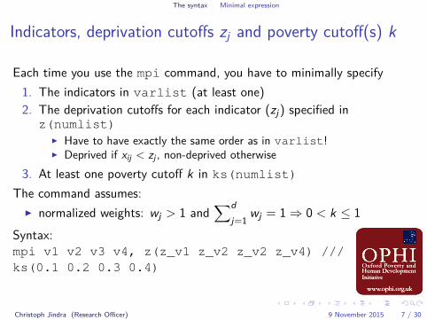
The syntax Minimal expression
Indicators, deprivation cutoffs zj and poverty cutoff(s) k
Each time you use the mpi command, you have to minimally specify1. The indicators in varlist (at least one)2. The deprivation cutoffs for each indicator (zj) specified in
z(numlist)I Have to have exactly the same order as in varlist!I Deprived if xij < zj , non-deprived otherwise
3. At least one poverty cutoff k in ks(numlist)The command assumes:
I normalized weights: wj > 1 and∑d
j=1wj = 1⇒ 0 < k ≤ 1
Syntax:mpi v1 v2 v3 v4, z(z_v1 z_v2 z_v2 z_v4) ///ks(0.1 0.2 0.3 0.4)
Christoph Jindra (Research Officer) 9 November 2015 7 / 30
The syntax Minimal expression
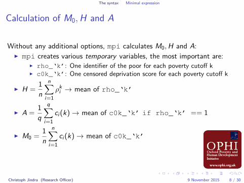
Calculation of M0, H and A
Without any additional options, mpi calculates M0,H and A:I mpi creates various temporary variables, the most important are:
I rho_‘k’: One identifier of the poor for each poverty cutoff kI c0k_‘k’: One censored deprivation score for each poverty cutoff k
I H = 1n
n∑i=1
ρki → mean of rho_‘k’
I A = 1q
q∑i=1
ci(k)→ mean of c0k_‘k’ if rho_‘k’ == 1
I M0 = 1n
n∑i=1
ci(k)→ mean of c0k_‘k’
Christoph Jindra (Research Officer) 9 November 2015 8 / 30
The syntax Minimal expression
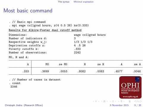
Most basic command
. // Basic mpi command
. mpi wage collgrad hours, z(4 0.5 26) ks(0.333)Results for Alkire-Foster dual cutoff method
Dimensions: wage collgrad hoursNumber of indicators d: 3Respective weights w_j: 1/3 1/3 1/3Deprivation cutoffs z: 4 .5 26Poverty cutoffs k: .333Number of observations: 2242M0, H and A:
k M0 se M0 H se H A se A
.333 .3699 .0053 .8082 .0083 .4577 .0046
. // Number of cases in dataset
. count2246
Christoph Jindra (Research Officer) 9 November 2015 9 / 30
The syntax Minimal expression
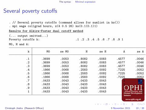
Several poverty cutoffs
. // Several poverty cutoffs (command allows for numlist in ks())
. mpi wage collgrad hours, z(4 0.5 26) ks(0.1(0.1)1)Results for Alkire-Foster dual cutoff method
(... output omitted...)Poverty cutoffs k: .1 .2 .3 .4 .5 .6 .7 .8 .9 1M0, H and A:
k M0 se M0 H se H A se A
.1 .3699 .0053 .8082 .0083 .4577 .0046
.2 .3699 .0053 .8082 .0083 .4577 .0046
.3 .3699 .0053 .8082 .0083 .4577 .0046
.4 .1866 .0068 .2583 .0092 .7225 .0052
.5 .1866 .0068 .2583 .0092 .7225 .0052
.6 .1866 .0068 .2583 .0092 .7225 .0052
.7 .0433 .0043 .0433 .0043 1 0
.8 .0433 .0043 .0433 .0043 1 0
.9 .0433 .0043 .0433 .0043 1 01 .0433 .0043 .0433 .0043 1 0
Christoph Jindra (Research Officer) 9 November 2015 10 / 30
The syntax Missing values
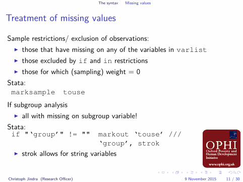
Treatment of missing values
Sample restrictions/ exclusion of observations:I those that have missing on any of the variables in varlistI those excluded by if and in restrictionsI those for which (sampling) weight = 0
Stata:marksample touse
If subgroup analysisI all with missing on subgroup variable!
Stata:if "‘group’" != "" markout ‘touse’ ///
‘group’, strok
I strok allows for string variables
Christoph Jindra (Research Officer) 9 November 2015 11 / 30
Options Weights
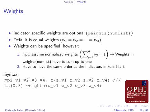
Weights
I Indicator specific weights are optional (weights(numlist))I Default is equal weights (w1 = w2 = ... = wd)I Weights can be specified, however:
1. mpi assume normalized weights(∑d
j=1wj = 1
)→ Weights in
weights(numlist) have to sum up to one2. Have to have the same order as the indicators in varlist
Syntax:mpi v1 v2 v3 v4, z(z_v1 z_v2 z_v2 z_v4) ///ks(0.3) weights(w_v1 w_v2 w_v3 w_v4)
Christoph Jindra (Research Officer) 9 November 2015 12 / 30
Options Weights
Weights
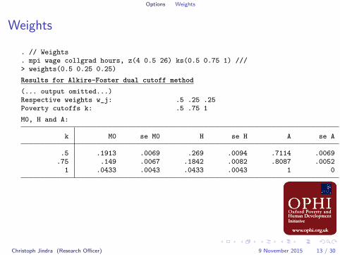
. // Weights
. mpi wage collgrad hours, z(4 0.5 26) ks(0.5 0.75 1) ///> weights(0.5 0.25 0.25)Results for Alkire-Foster dual cutoff method
(... output omitted...)Respective weights w_j: .5 .25 .25Poverty cutoffs k: .5 .75 1M0, H and A:
k M0 se M0 H se H A se A
.5 .1913 .0069 .269 .0094 .7114 .0069.75 .149 .0067 .1842 .0082 .8087 .0052
1 .0433 .0043 .0433 .0043 1 0
Christoph Jindra (Research Officer) 9 November 2015 13 / 30
Options Multidimensional FGT class
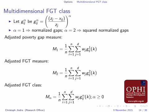
Multidimensional FGT classI Let gαij be gαij =
((zj − xij)
zj
)αI α = 1⇒ normalized gaps; α = 2⇒ squared normalized gaps
Adjusted poverty gap measure:
M1 = 1n
n∑i=1
d∑j=1
wjg1ij (k)
Adjusted FGT measure:
M2 = 1n
n∑i=1
d∑j=1
wjg2ij (k)
Adjusted FGT class:
Mα = 1n
n∑i=1
d∑j=1
wjgαij (k);α ≥ 0
Christoph Jindra (Research Officer) 9 November 2015 14 / 30
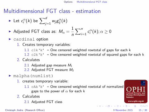
Options Multidimensional FGT class
Multidimensional FGT class - estimationI Let cαi (k) be
∑dj=1
wjgαij (k)
I Adjusted FGT class as: Mα = 1n∑n
i=1cαi (k);α ≥ 0
I cardinal option1. Creates temporary variables:
1.1 c1k‘k’ = One censored weighted rowtotal of gaps for each k1.2 c2k‘k’ = One censored weighted rowtotal of squared gaps for each k
2. Calculates2.1 Adjusted gap measure M12.2 Adjusted FGT measure M2
I malpha(numlist)1. creates temporary variable:
1.1 cAk‘k’ = One censored weighted rowtotal of normalizedgaps to the power of α for each k
2. Calculates2.1 Adjusted FGT class
Christoph Jindra (Research Officer) 9 November 2015 15 / 30
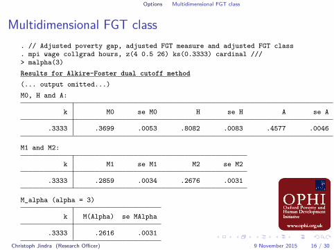
Options Multidimensional FGT class
Multidimensional FGT class. // Adjusted poverty gap, adjusted FGT measure and adjusted FGT class. mpi wage collgrad hours, z(4 0.5 26) ks(0.3333) cardinal ///> malpha(3)Results for Alkire-Foster dual cutoff method
(... output omitted...)M0, H and A:
k M0 se M0 H se H A se A
.3333 .3699 .0053 .8082 .0083 .4577 .0046
M1 and M2:
k M1 se M1 M2 se M2
.3333 .2859 .0034 .2676 .0031
M_alpha (alpha = 3)
k M(Alpha) se MAlpha
.3333 .2616 .0031
Christoph Jindra (Research Officer) 9 November 2015 16 / 30
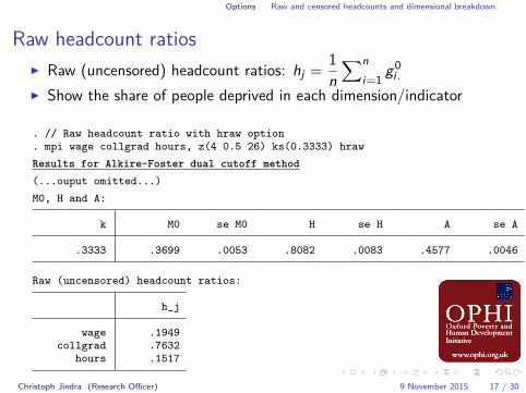
Options Raw and censored headcounts and dimensional breakdown
Raw headcount ratiosI Raw (uncensored) headcount ratios: hj = 1
n∑n
i=1g0
i .I Show the share of people deprived in each dimension/indicator
. // Raw headcount ratio with hraw option
. mpi wage collgrad hours, z(4 0.5 26) ks(0.3333) hrawResults for Alkire-Foster dual cutoff method
(...ouput omitted...)M0, H and A:
k M0 se M0 H se H A se A
.3333 .3699 .0053 .8082 .0083 .4577 .0046
Raw (uncensored) headcount ratios:
h_j
wage .1949collgrad .7632
hours .1517
Christoph Jindra (Research Officer) 9 November 2015 17 / 30
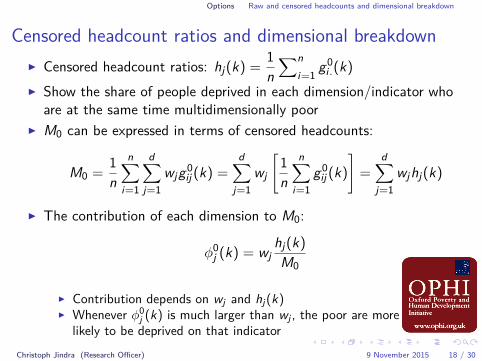
Options Raw and censored headcounts and dimensional breakdown
Censored headcount ratios and dimensional breakdownI Censored headcount ratios: hj(k) = 1
n∑n
i=1g0
i .(k)I Show the share of people deprived in each dimension/indicator who
are at the same time multidimensionally poorI M0 can be expressed in terms of censored headcounts:
M0 = 1n
n∑i=1
d∑j=1
wjg0ij (k) =
d∑j=1
wj
[1n
n∑i=1
g0ij (k)
]=
d∑j=1
wjhj(k)
I The contribution of each dimension to M0:
φ0j (k) = wjhj(k)M0
I Contribution depends on wj and hj(k)I Whenever φ0j (k) is much larger than wj , the poor are more
likely to be deprived on that indicatorChristoph Jindra (Research Officer) 9 November 2015 18 / 30
Options Raw and censored headcounts and dimensional breakdown
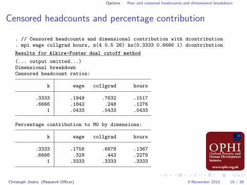
Censored headcounts and percentage contribution
. // Censored headcounts and dimensional contribution with dcontribution
. mpi wage collgrad hours, z(4 0.5 26) ks(0.3333 0.6666 1) dcontributionResults for Alkire-Foster dual cutoff method
(... output omitted...)Dimensional breakdownCensored headcount ratios:
k wage collgrad hours
.3333 .1949 .7632 .1517
.6666 .1842 .248 .12761 .0433 .0433 .0433
Percentage contribution to M0 by dimensions:
k wage collgrad hours
.3333 .1756 .6878 .1367
.6666 .329 .443 .22791 .3333 .3333 .3333
Christoph Jindra (Research Officer) 9 November 2015 19 / 30
Options Subgroup analysis
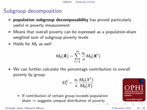
Subgroup decompositionI population subgroup decomposability has proved particularly
useful in poverty measurementI Means that overall poverty can be expressed as a population-share
weighted sum of subgroup poverty levelsI Holds for M0 as well:
M0(X) =m∑`=1
n`n M0(X`)
I We can further calculate the percentage contribution to overallpoverty by group:
D0` = n`
nM0(X `)M0(X )
I If contribution of certain group exceeds populationshare ⇒ suggests unequal distribution of poverty
Christoph Jindra (Research Officer) 9 November 2015 20 / 30
Options Subgroup analysis
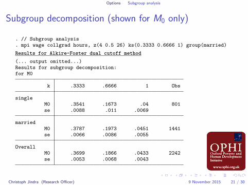
Subgroup decomposition (shown for M0 only)
. // Subgroup analysis
. mpi wage collgrad hours, z(4 0.5 26) ks(0.3333 0.6666 1) group(married)Results for Alkire-Foster dual cutoff method
(... output omitted...)Results for subgroup decomposition:for M0
k .3333 .6666 1 Obs
singleM0 .3541 .1673 .04 801se .0088 .011 .0069
marriedM0 .3787 .1973 .0451 1441se .0066 .0086 .0055
OverallM0 .3699 .1866 .0433 2242se .0053 .0068 .0043
Christoph Jindra (Research Officer) 9 November 2015 21 / 30
Options Subgroup analysis
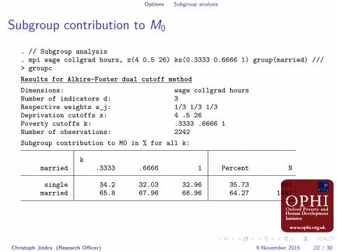
Subgroup contribution to M0
. // Subgroup analysis
. mpi wage collgrad hours, z(4 0.5 26) ks(0.3333 0.6666 1) group(married) ///> groupcResults for Alkire-Foster dual cutoff method
Dimensions: wage collgrad hoursNumber of indicators d: 3Respective weights w_j: 1/3 1/3 1/3Deprivation cutoffs z: 4 .5 26Poverty cutoffs k: .3333 .6666 1Number of observations: 2242Subgroup contribution to M0 in % for all k:
kmarried .3333 .6666 1 Percent N
single 34.2 32.03 32.96 35.73 801married 65.8 67.96 66.96 64.27 1441
Christoph Jindra (Research Officer) 9 November 2015 22 / 30
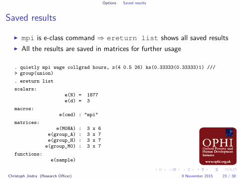
Options Saved results
Saved results
I mpi is e-class command ⇒ ereturn list shows all saved resultsI All the results are saved in matrices for further usage
. quietly mpi wage collgrad hours, z(4 0.5 26) ks(0.33333(0.33333)1) ///> group(union). ereturn listscalars:
e(N) = 1877e(d) = 3
macros:e(cmd) : "mpi"
matrices:e(M0HA) : 3 x 6
e(group_A) : 3 x 7e(group_H) : 3 x 7
e(group_M0) : 3 x 7functions:
e(sample)
Christoph Jindra (Research Officer) 9 November 2015 23 / 30
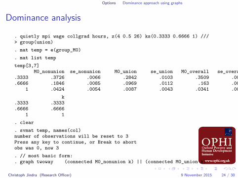
Options Dominance approach using graphs
Dominance analysis
. quietly mpi wage collgrad hours, z(4 0.5 26) ks(0.3333 0.6666 1) ///> group(union). mat temp = e(group_M0). mat list temptemp[3,7]
M0_nonunion se_nonunion M0_union se_union M0_overall se_overall.3333 .3726 .0066 .2842 .0103 .3509 .0056.6666 .1846 .0085 .0969 .0112 .163 .0071
1 .0424 .0054 .0087 .0043 .0341 .0042k
.3333 .3333
.6666 .66661 1
. clear
. svmat temp, names(col)number of observations will be reset to 3Press any key to continue, or Break to abortobs was 0, now 3. // most basic form:. graph twoway (connected M0_nonunion k) || (connected M0_union k)
Christoph Jindra (Research Officer) 9 November 2015 24 / 30
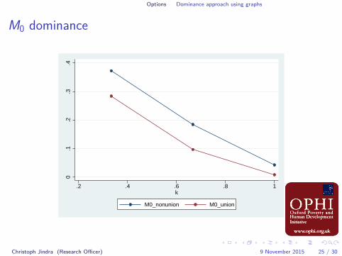
Options Dominance approach using graphs
M0 dominance
0.1
.2.3
.4
.2 .4 .6 .8 1k
M0_nonunion M0_union
Christoph Jindra (Research Officer) 9 November 2015 25 / 30
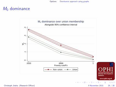
Options Dominance approach using graphs
M0 dominance
0.1
.2.3
.4M
0
.3333 .6666 1Poverty cutoff k
Non−union Union
Alongside 95% confidence intervalM0 dominance over union membership
Christoph Jindra (Research Officer) 9 November 2015 26 / 30

To do list
do’s
I More options if necessary (creating actual variables)?I WarningsI Complete list of returned resultsI Rounding and precisionI Testing/verification based on Gould (2001)
I Testing procedures forI M0, H and AI M1 and M2I Raw headcounts and censored headcounts already implemented
I But needs to be implemented for all elementsI Complex survey design
I Will be implemented using svy optionI Will use the default: linearized variance estimator
Christoph Jindra (Research Officer) 9 November 2015 27 / 30
To do list
don’ts: BootstrappingI Often applied, but is it really that easy? “Examples where the
bootstrap fails are abundant [...]. Complex survey data is one suchexample” (Kolenikov, 2010)
I In case of only few PSUs per stratum, naive bootstrapping can leadto biased and inconsistent variance estimates
I Replicate weights have to be used for correct estimation (Asparouhovand Muthén, 2010; Kolenikov, 2010)
I ≈ bootstrap samples that can be used to assess the variability of theestimates
I Often not delivered with datasetI Can theoretically be calculated if one understands the sampling
procedure correctly (package bsweights)I In Stata: svy bootstrap requires that the bootstrap
replicate weights be identified (StataCorp, 2013, p. 74)I No option, but can theoretically be calculated
Christoph Jindra (Research Officer) 9 November 2015 28 / 30

To do list
Bootstrapping without complex survey design
Christoph Jindra (Research Officer) 9 November 2015 29 / 30
Literature
Literature I
Abdelkrim, A. and J.-Y. Duclos (2013). User Manual for Stata Package DASP: Version2.3. PEP, World Bank, UNDP and University Laval.
Alkire, S. and J. Foster (2011). Counting and multidimensional poverty measurement.Journal of Public Economics 95(7-8), 476–487.
Asparouhov, T. and B. O. Muthén (2010). Resampling Methods in Mplus for ComplexSurvey Data.
Gould, W. (2001). Statistical software certification. The Stata Journal 1(1), 29–50.Kolenikov, S. (2010). Resampling variance estimation for complex survey data. The
Stata Journal 10(2), 165–199.StataCorp (2013). Stata Survey Data Reference Manual - Release 13. College Station,
Texas: Stata Press.
Christoph Jindra (Research Officer) 9 November 2015 30 / 30