mqbench: towards reproducible and deployable model

MQBench: Towards Reproducible and DeployableModel Quantization Benchmark

Yuhang Li∗, Mingzhu Shen∗, Jian Ma∗, Yan Ren∗, Mingxin Zhao∗,Qi Zhang∗, Ruihao Gong∗, Fengwei Yu, Junjie Yan

SenseTime Researchhttp://mqbench.tech/

Abstract

Model quantization has emerged as an indispensable technique to accelerate deeplearning inference. While researchers continue to push the frontier of quantizationalgorithms, existing quantization work is often unreproducible and undeployable.This is because researchers do not choose consistent training pipelines and ignorethe requirements for hardware deployments. In this work, we propose ModelQuantization Benchmark (MQBench), a first attempt to evaluate, analyze, andbenchmark the reproducibility and deployability for model quantization algorithms.We choose multiple different platforms for real-world deployments, including CPU,GPU, ASIC, DSP, and evaluate extensive state-of-the-art quantization algorithmsunder a unified training pipeline. MQBench acts like a bridge to connect thealgorithm and the hardware. We conduct a comprehensive analysis and findconsiderable intuitive or counter-intuitive insights. By aligning the training settings,we find existing algorithms have about the same performance on the conventionalacademic track. While for the hardware-deployable quantization, there is a hugeaccuracy gap which remains unsettled. Surprisingly, no existing algorithm winsevery challenge in MQBench, and we hope this work could inspire future researchdirections.

1 IntroductionModern deep learning is increasingly consuming larger memory and computation to pursue higherperformance. While large-scale models can be trained on the cloud, transition to edge devices duringdeployment is notoriously hard due to the limited resource budget, including latency, energy andmemory consumption. For this reason various techniques have been developed to accelerate the deeplearning inference, including model quantization [1, 2, 3, 4, 5], pruning [6, 7, 8, 9, 10], neural networkdistillation [11, 12], lightweight network design [13], and weight matrix decomposition [14].

In this work, we focus on model quantization for efficient inference. Quantization targets to mapthe (nearly) continuous 32-bit floating-point (FP) numbers into discrete low-bit integers. As a result,the neural networks could rely on the integer-arithmetic units to speed up the inference. In academicresearch, there is a trend towards steadily reducing the bit-width and maintaining the accuracy across arange of quantized network architectures on ImageNet. It is incredible that the even 3-bit quantizationof both weights and activations can reach FP-level accuracy [15]. Exciting though the breakthroughis, there lacks a systematic study that whether these research works can really be applied to practice,and whether the major improvement is brought by the algorithm rather than the training techniques.

We point out two long-neglected key factors in quantization research, namely reproducibility anddeployability. First, we observe that the training hyper-parameters can significantly affect theperformance of a quantized network. As an example, Esser et al. [15] adopt cosine annealed learning∗Equal Contributions. Correspondence to Yuhang Li <[email protected]>, Ruihao Gong <gongrui-

[email protected]>.

35th Conference on Neural Information Processing Systems (NeurIPS 2021) Track on Datasets and Benchmarks.

arX

iv:2

111.

0375

9v1

[cs

.LG

] 5

Nov

202

1

http://mqbench.tech/

Target Hardware Devices

CPU

Quantization Algorithms

QuantizationAwareTraining

PostTraining

Quantization

MQBench

BenchmarkingReproducibleAlgorithms

BenchmarkingDeployableHardwareGPU ASIC DSP

Problems Others MQBench

Rep

rodu

ce Unified Hyper-parameters 7 3Unified Training Pipelines 7 3Diverse Architectures 7 3Open Source k 3

Dep

loy # Supported Hardware 0 or 1 5

Hardware Quantizer k 3Fold BN k 3Graph Alignments 7 3

Figure 1 & Table 1: Left: The placement of MQBench, which connects the algorithms and hardware. Right:comparison between MQBench and other quantization works. 3: condition satisfied, 7: condition not satisfied,k: condition satisfied only in part of existing work.

rate [16] and better weight decay choice, improving the Top-1 accuracy of 2-bit ResNet-18 [17]by 0.7% and 0.4% on ImageNet. Full precision network pre-training can also boost quantizationresults [15,18]. The reproducibility issue has received considerable attention in other areas as well, e.g.NAS-Bench-101 [19]. So far, there lacks a benchmark that unifies training pipelines and comparesthe quantization algorithms in a thorough and impartial sense.

Second, we find that the majority of the academic research papers do not test their algorithms onreal hardware devices. As a result, the reported performance may not be reliable. For one thing,hardware will fold Batch Normalization (BN) layers [20] into convolutional layers [3] to avoidadditional overhead. But most research papers just keep BN layers intact. For another, research paperonly considers quantizing the input and weights parameters of the convolutional layers. While indeployment the whole computational graph should be quantized. These rules will inevitably makequantization algorithms less resilient. Another less studied problem is the algorithm robustness: Whatwill happen if one algorithm is applied to per-channel quantization but it is designed to per-tensorquantization at first? The algorithm should incorporate the diversity of quantizers design. All theseproblems suggest a large gap between academic research and real-world deployments.

In this work, we propose Model Quantization Benchmark (MQBench), a framework designed toanalyze and reproduce quantization algorithms on several real-world hardware environments (SeeFig. 1 & Table 1). We carefully studied existing quantization algorithms and hardware deploymentsettings to set up a bridge between the algorithms and hardware. To complete MQBench, we utilizeover 50 GPU years of computation time, in an effort to foster both reproducibility and deployabilityin quantization research. Meanwhile, our benchmark offers some overlooked observations which mayguide further research. To our best knowledge, this is the first work that benchmarks quantizationalgorithms on multiple general hardware platforms.

In the following context of this paper, we first build a benchmark for reproducing algorithms underunified training settings in Sec. 2. We introduce the requirements for hardware deployable quantizationin Sec. 3. Then we conduct extensive experimental evaluation and analysis in Sec. 5. Due to thespace limit, we put related work as well as the visualization results in the Appendix.

2 MQBench: Towards Reproducible Quantization

In this section, we benchmark the reproducibility of quantization algorithms, mainly includingQuantization-Aware Training (QAT)2. We evaluate the performance of algorithms on ImageNet [21]classification task. Other tasks like detection, segmentation and language applications are notconsidered for now since few baseline algorithms were proposed. MQBench evaluation is performedin 4 dimensions: supported inference library given a specific hardware, quantization algorithm,network architecture, and bit-width.

Hardware-aware Quantizer. Throughout the paper, we mainly consider uniform quantization,since the non-uniform quantization requires special hardware design. We use w and x to denote theweight matrix and activation matrix in a neural network. A complete uniform quantization processincludes quantization operation and de-quantization operation, which can be formulated by:

w = clip(⌊ws

⌉+ z,Nmin, Nmax), w = s · (w − z) (1)

2We also build an equally thoroughgoing benchmark for Post-Training Quantization (PTQ) in Appendix. C.

2

Table 2: Comparison of (1) the different hardware we selected and (2) the different QAT algorithms. Infer. Lib.is the inference library; FBN means whether fold BN. k means undeployable originally, but can be deployablewhen certain requirements are satisfied.

Infer. Lib. Provider HW Type Hardware s Form. Granularity Symmetry Graph FBNTensorRT [22] NVIDIA GPU Tesla T4/P4 FP32 Per-channel Symmetric 2 3ACL [23] HUAWEI ASIC Ascend310 FP32 Per-channel Asymmetric 1 3TVM [25] OctoML CPU ARM POT Per-tensor Symmetric 3 3SNPE [24] Qualcomm DSP Snapdragon FP32 Per-tensor Asymmetric 3 3FBGEMM [26] Facebook CPU X86 FP32 Per-channel Asymmetric 3 3

Algorithms Deployable Uniformity Quant. Type s Form. Granularity Symmetry Graph FBNLSQ [15] k Uniform learning-based FP32 Per-tensor Symmetric 1 7APoT [27] 7 Non-uniform learning-based FP32 Per-tensor Symmetric 1 7QIL [18] 7 Uniform learning-based FP32 Per-tensor Symmetric 1 7DSQ [28] k Uniform rule-based FP32 Per-tensor Symmetric 1 7LQ-Net [29] 7 Non-uniform rule-based FP32 Per-tensor Symmetric 1 7PACT [30] k Uniform learning+rule FP32 Per-tensor Symmetric 1 7DoReFa [31] k Uniform rule-based FP32 Per-tensor Symmetric 1 7

where s ∈ R+ and z ∈ Z are called scale and zero-point, respectively. b·e rounds the continuousnumbers to nearest integers. Eq. (1) first quantizes the weights or activations into target integerrange [Nmin, Nmax] and then de-quantizes the integers to original range. Given t bits, the rangeis determined by [−2t−1, 2t−1 − 1]. We can divide the quantizer based on several metrics: (1)Symmetric or asymmetric quantization: For symmetric quantization the zero-point is fixed to 0, whilethe asymmetric quantization has an adjustable zero-point to adapt different range; (2) Per-tensoror per-channel quantization: The per-tensor quantization uses only one set of scale and zero-pointfor a tensor in one layer while per-channel quantization quantizes each weight kernel independently(i.e. for each row of weight matrix: wi,:); (3) FP32 (32-bit Floating Point) scale or POT (Power ofTwo) scale: FP32 scale is nearly continuous, while power-of-two scale is much more challenging.However, POT scale may offer further speed-up.

We select 5 general hardware libraries to evaluate the quantization algorithms, including NVIDIA’sTensorRT [22] for Graphics Processing Unit (GPU) inference, HUAWEI’s ACL [23] for Application-Specific Integrated Circuit (ASIC) inference, Qualcomm’s SNPE [24] for mobile Digital SignalProcessor (DSP), TVM [25] for ARM Central Processing Unit (CPU), FBGEMM [26] for X86server-side CPU. We summarize their implementation details for quantization in Table 2 upper side.Each hardware setting corresponds to a unique quantizer design. Thus, the developed algorithmmust be robust to adapt different quantizer configurations. We put the detailed setup for hardwareenvironments in Appendix. E.

Algorithm. For quantization-aware training, we compare 6 different algorithms [15,18,27,28,29,30,31]. However, several algorithms cannot be deployable even if we align the quantizer configurationand the other requirements. We put the summary of them in Table 2 lower side. All these algorithmsuse per-tensor, symmetric settings. We refer this type as academic setting. We also identify thequantizer type as learning-based, which learns the scale, or rule-based, which directly computes thescale with heuristics. For a detailed description of these algorithms and the reason why they can beextended to deployable quantization, please see Appendix. F.

Network Architecture. We choose ResNet-18 and ResNet-50 [17] as they are most widely usedbaseline architectures. We also adopt MobileNetV2 [13] which is a lightweight architecture withdepthwise separable convolution. In order to quantize EfficientNet [32], we leverage its Lite ver-sion [33] that excludes the squeeze-and-excitation block and replaces swish activation to ReLU6for better integer numeric support on hardware. Finally, we add an another advanced architectureRegNetX-600MF [34] with group convolution.

Bit-width. In this paper, we mainly experiment with 8-bit post-training quantization (Appendix.C) and 4-bit quantization-aware training. To test the accuracy of the quantized model, we simulatethe algorithm with fake quantization (see difference between fake and real quantization in Sec. 3.1).Unlike the reported results in other paper, 4-bit QAT in our benchmark could be very challenging.We do not experiment with 3-bit quantization because it is undeployable on general hardware. As for2-bit quantization, we find most of the algorithms do not converge on hardware settings.

3

Dequan'ze

Dequantize

Conv ReLU𝒚𝒍

𝒙𝒍$𝟏Quantize

𝒘𝒍$𝟏

Quan'ze

𝒙'𝒍

𝒘'𝒍

𝒙(𝒍$𝟏

𝒘(𝒍$𝟏

FP32FP32

FP32 FP32 FP32 FakeQuantize𝒙'𝒍$𝟏

𝒘'𝒍$𝟏

FP32

FP32+𝒃FP32

(a) Fake quantization for simulated-training.

𝒙"𝒍

𝒘"𝒍Conv ReLU

𝒚𝒍𝒙&𝒍'𝟏 Quan,ze

𝒘𝒍'𝟏

Quantize(offline)

𝒙"𝒍'𝟏

𝒘"𝒍'𝟏Dequantize

𝒙𝒍'𝟏

INT8

INT8 INT32INT32 INT8

INT8

Requantize

+𝑧+𝑧, − 𝑧+𝒙" − 𝑧,𝒘"+𝒃" INT32

(b) Real quantization in deployments.

Figure 2: Example computation diagram of a single 8-bit quantized convolutional layer in GPU training or realhardware deployments.

2.1 Training Pipelines and Hyper-parameters

Early work like [30, 31] trains the quantized model from scratch, which may have inferior accuracythan fine-tuning [35]. Besides, each paper may have different pre-trained models for initialization.In MQBench, we adopt fine-tuning for all algorithms and each model is initialized by the samepre-trained model, eliminating the inconsistency at initialization.

We adopt standard data prepossessing for training data, including RandomResizeCrop to 224 res-olution, RandomHorizontalFlip, ColorJitter with brightness= 0.2, contrast= 0.2, saturation

Table 3: Training hyper-parameters. Batch Size isthe batch size per GPU. * means 0 weight decay forBN parameters.

Model LR L2 Reg. Batch Size # GPU

ResNet-18 0.004 10−4 64 8ResNet-50 0.004 10−4 16 16EffNet&MbV2 0.01 10−5* 32 16RegNet 0.004 4× 10−5 32 16

= 0.2, and hue= 0.1. The test data is centeredcropped to 224 resolution. We use 0.1 label smooth-ing in training to add regularization. No other ad-vanced augmentations are further adopted. All mod-els are trained for 100 epochs, with a linear warm-up in the first epoch. The learning rate is decayedby cosine annealing policy [16]. We use the SGDoptimizer for training, with 0.9 momentum and Nes-terov updates. Other training hyper-parameters canbe found in Table 3 aside. We discuss our choice of this set of hyper-parameter in the Appendix. A.

3 MQBench: Towards Deployable Quantization

3.1 Fake and Real Quantization

Given a weight matrix w and an activation matrix x, the product is given by

yij =

n∑k=1

wikxkj︸︷︷︸Fake Quantize

= swsx

n∑k=1

(wikxkj − zwxkj − zxwik + zwzx)︸︷︷︸Real Quantize

, (2)

where y is the convolution output or the pre-activation. In order to perform QAT on GPU, we haveto simulate the quantization function with FP32, denoted as the left Fake Quantize bracket. For thepractical inference acceleration, we have to utilize integer-arithmetic-only [3], denoted as the rightReal Quantize bracket. In Fig. 2, we draw the computational graph of fake quantization and realquantization to reveal their relationship.

For fake quantization, the weights and input activations are quantized and de-quantized beforeconvolution. The intermediate results as well as the bias term, are all simulated with FP32.

As for deployments in real-world, the computation in the Real Quantize bracket is integer-only and isaccumulated using INT32. One can further optimize the convolution kernels by performing the lasttwo terms offline, since w and zw, zx are determined prior to deployment [36]. For bias parameters,we can keep them in INT32, quantized by b = bb/sbe, where b is INT32 and sb = swsx. As a result,the bias can be easily fused into Eq. (2). Then, the de-quantization will do the scaling outside thebracket. In the deployment, the de-quantization of the output and the further quantization to integersis fused together, called Requantization, given by

xl+1 = swl · sxl · xl+1, xl+1 = clip(

⌊xl+1

sxl+1

⌉+ zxl+1 , Nmin, Nmax) (3)

We should point out that these two graphs may have some tiny and unavoidable disparity, mainlyresulting from the difference between FP32 in simulation and real integers in deployments.

4

Conv

𝒙"

ReLU+Quant

𝒘

Fold𝒘𝛾𝜎

FQuant

𝒘"&'()

𝒛+

+𝒃&'()Conv

𝒙"

ReLU+Quant

𝒘

Fold𝜇/𝜎/

FQuant

𝒘"&'()

𝒛+

+𝒃1&'()

Conv

𝒘𝛾𝜎/

Conv

𝒙"

ReLU+Quant

𝒘

Fold

FQuant

𝒘"&'()

𝒛+

+𝒃1&'()

Conv

𝒘𝛾𝜎

𝜇/𝜎/

×𝜎𝜎/

Conv

𝒙"

ReLU+Quant

𝒘

Fold

FQuant

𝒘"&'()

𝒛+

𝒘𝛾𝜎

×𝜎𝛾

BatchNorm

(a) (b) (c) (d) (e)

Update

Conv

𝒙"

ReLU+Quant

𝒘&'()

FQuant

𝒘"&'()

𝒛+

+𝒃&'()

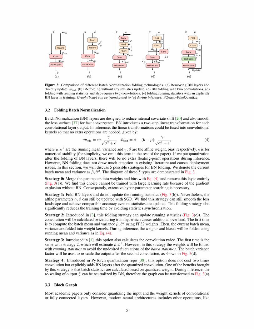
Figure 3: Comparison of different Batch Normalization folding technologies. (a) Removing BN layers anddirectly update wfold. (b) BN folding without any statistics update. (c) BN folding with two convolutions. (d)folding with running statistics and also requires two convolutions. (e) folding running statistics with an explicitlyBN layer in training. Graph (bcde) can be transformed to (a) during inference. FQuant=FakeQuantize.

3.2 Folding Batch Normalization

Batch Normalization (BN) layers are designed to reduce internal covariate shift [20] and also smooththe loss surface [37] for fast convergence. BN introduces a two-step linear transformation for eachconvolutional layer output. In inference, the linear transformations could be fused into convolutionalkernels so that no extra operations are needed, given by:

wfold = wγ√σ2 + ε

, bfold = β + (b− µ)γ√σ2 + ε

, (4)

where µ, σ2 are the running mean, variance and γ, β are the affine weight, bias, respectively. ε is fornumerical stability (for simplicity, we omit this term in the rest of the paper). If we put quantizationafter the folding of BN layers, there will be no extra floating-point operations during inference.However, BN folding does not draw much attention in existing literature and causes deploymentissues. In this section, we will discuss 5 possible strategies for BN folding. We denote the currentbatch mean and variance as µ, σ2. The diagram of these 5 types are demonstrated in Fig. 3.

Strategy 0: Merge the parameters into weights and bias with Eq. (4), and remove this layer entirely(Fig. 3(a)). We find this choice cannot be trained with large learning rate because of the gradientexplosion without BN. Consequently, extensive hyper-parameter searching is necessary.

Strategy 1: Fold BN layers and do not update the running statistics (Fig. 3(b)). Nevertheless, theaffine parameters γ, β can still be updated with SGD. We find this strategy can still smooth the losslandscape and achieve comparable accuracy even no statistics are updated. This folding strategy alsosignificantly reduces the training time by avoiding statistics synchronization.

Strategy 2: Introduced in [3], this folding strategy can update running statistics (Fig. 3(c)). Theconvolution will be calculated twice during training, which causes additional overhead. The first timeis to compute the batch mean and variance µ, σ2 using FP32 weights. Then, the current batch mean,variance are folded into weight kernels. During inference, the weights and biases will be folded usingrunning mean and variance as in Eq. (4).

Strategy 3: Introduced in [1], this option also calculates the convolution twice. The first time is thesame with strategy 2, which will estimate µ, σ2. However, in this strategy the weights will be foldedwith running statistics to avoid the undesired fluctuations of the batch statistics. The batch variancefactor will be used to re-scale the output after the second convolution, as shown in Fig. 3(d).

Strategy 4: Introduced in PyTorch quantization repo [38], this option does not cost two timesconvolution but explicitly adds BN layers after the quantized convolution. One of the benefits broughtby this strategy is that batch statistics are calculated based on quantized weight. During inference, there-scaling of output σγ can be neutralized by BN, therefore the graph can be transformed to Fig. 3(a).

3.3 Block Graph

Most academic papers only consider quantizing the input and the weight kernels of convolutionalor fully connected layers. However, modern neural architectures includes other operations, like

5

Downsample Downsample

Conv

𝒙𝒍

FakeQuant

+

ReLU

FakeQuant

Conv

ReLU

𝒙$𝒍

ReLU

FakeQuant

Conv

ReLU

Conv

FakeQuant

𝒙$𝒍

ReLU

FakeQuant

Conv

ReLU

Conv

FakeQuant

FakeQuant

Conv

FakeQuant

Conv

FakeQuant

Downsample

Conv

FakeQuant

+ +

Quan/za/on

Dequan/za/on

（1）（2）（3）

Figure 4: Comparison of different quantization implementations for a basic block in the ResNet [17].elementwise-add in ResNet [17] and concatenation in InceptionV3 [39]. In addition, differenthardware will consider different levels of graph optimization and can propose different solutions toconstruct a graph for quantized neural networks. In MQBench, we sort out different implementationsand summarize them in a schematic diagram (Fig. 4). Note that Fig. 4 only gives an example ofa basic block in ResNet-18/-34. The bottleneck block in ResNet-50 can be naturally derived fromthis diagram. We also put the diagram of the inverted residual bottleneck of MobileNetV2 [13], andconcatenation quantization in the Appendix. G.

Fig. 4 left shows the conventional academic implementations for quantizing a basic block. Only theinput of convolutional layers will be quantized to 8-bit. (Note that in academic papers the INT8 meansboth quantization and de-quantization.) The block input and output as well as the elementwise-addall operate at full precision. Consequently, the network throughput hasn’t been reduced, and willsignificantly affect the latency. In some architectures, this graph even won’t bring any accelerationsince the latency is dominated by I/O. Another problem is the separate quantization of the activationin the downsample block, which also brings undesired costs.

Fig. 4 middle presents the NVIDIA’s TensorRT [22] implementation for basic block. We can findthat the input and output must be quantized to low-bit to reduce the data throughput. Low bit inputcan ensure two branches will use the same quantized activation in the downsample block. As forthe elementwise-add layer, it will be conducted in a 32-bit mode due to the fusion with one of theformer convolutional layer’s bias addition. Thus only one of its inputs will be quantized. Fig. 4 rightdemonstrates the implementation in other hardware library, such as FBGEMM [26] and TVM [25].The only difference is that they require all inputs of the elementwise-add to be quantized. In 4-bitsymmetric quantization, this can severely affect the accuracy.

4 MQBench Implementation

We implement MQBench with Pytorch [40] package, with the support of the latest feature, thetorch.fx (also known as FX, see documentation in [41]) in version 1.8. FX contains a symbolictracer, an intermediate representation, and Python code generation, which allows for deeper metaprogramming. We implement the quantization algorithms and the hardware-aware configurations inMQBench. Only an API call is needed to trace a full precision model and convert it to a quantizedmodel. A code demo of quantizing ResNet-18 with TensorRT backend is presented in , For moredetails, readers are recommended to see the official repository.

5 MQBench Evaluation

In this section, we conduct a thorough evaluation and analysis for quantization algorithms, networkarchitectures, and hardware. We study several evaluation metrics, given by À test accuracy: the Top-1 accuracy on the ImageNet validation set, it directly reflects the task performance of the algorithm; Áhardware gap: the difference between hardware and academic test accuracy, this metric can reflectthe impact of deployable quantization on the algorithm; Â hardware robustness: the average testaccuracy on 5 hardware environments. Ã architecture robustness: the average test accuracy on 5network architectures. These last two metrics are often neglected by most of the existing literature but

6

https://github.com/ModelTC/MQBench

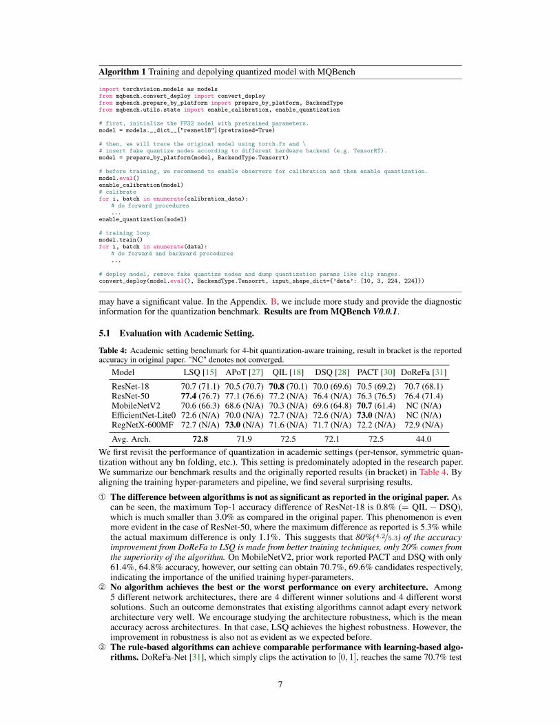
Algorithm 1 Training and depolying quantized model with MQBench

import torchvision.models as modelsfrom mqbench.convert_deploy import convert_deployfrom mqbench.prepare_by_platform import prepare_by_platform, BackendTypefrom mqbench.utils.state import enable_calibration, enable_quantization

# first, initialize the FP32 model with pretrained parameters.model = models.__dict__["resnet18"](pretrained=True)

# then, we will trace the original model using torch.fx and \# insert fake quantize nodes according to different hardware backend (e.g. TensorRT).model = prepare_by_platform(model, BackendType.Tensorrt)

# before training, we recommend to enable observers for calibration and then enable quantization.model.eval()enable_calibration(model)# calibratefor i, batch in enumerate(calibration_data):

# do forward procedures...

enable_quantization(model)

# training loopmodel.train()for i, batch in enumerate(data):

# do forward and backward procedures...

# deploy model, remove fake quantize nodes and dump quantization params like clip ranges.convert_deploy(model.eval(), BackendType.Tensorrt, input_shape_dict={’data’: [10, 3, 224, 224]})

may have a significant value. In the Appendix. B, we include more study and provide the diagnosticinformation for the quantization benchmark. Results are from MQBench V0.0.1.

5.1 Evaluation with Academic Setting.

Table 4: Academic setting benchmark for 4-bit quantization-aware training, result in bracket is the reportedaccuracy in original paper. "NC" denotes not converged.

Model LSQ [15] APoT [27] QIL [18] DSQ [28] PACT [30] DoReFa [31]

ResNet-18 70.7 (71.1) 70.5 (70.7) 70.8 (70.1) 70.0 (69.6) 70.5 (69.2) 70.7 (68.1)ResNet-50 77.4 (76.7) 77.1 (76.6) 77.2 (N/A) 76.4 (N/A) 76.3 (76.5) 76.4 (71.4)MobileNetV2 70.6 (66.3) 68.6 (N/A) 70.3 (N/A) 69.6 (64.8) 70.7 (61.4) NC (N/A)EfficientNet-Lite0 72.6 (N/A) 70.0 (N/A) 72.7 (N/A) 72.6 (N/A) 73.0 (N/A) NC (N/A)RegNetX-600MF 72.7 (N/A) 73.0 (N/A) 71.6 (N/A) 71.7 (N/A) 72.2 (N/A) 72.9 (N/A)

Avg. Arch. 72.8 71.9 72.5 72.1 72.5 44.0We first revisit the performance of quantization in academic settings (per-tensor, symmetric quan-tization without any bn folding, etc.). This setting is predominately adopted in the research paper.We summarize our benchmark results and the originally reported results (in bracket) in Table 4. Byaligning the training hyper-parameters and pipeline, we find several surprising results.

À The difference between algorithms is not as significant as reported in the original paper. Ascan be seen, the maximum Top-1 accuracy difference of ResNet-18 is 0.8% (= QIL − DSQ),which is much smaller than 3.0% as compared in the original paper. This phenomenon is evenmore evident in the case of ResNet-50, where the maximum difference as reported is 5.3% whilethe actual maximum difference is only 1.1%. This suggests that 80%(4.2/5.3) of the accuracyimprovement from DoReFa to LSQ is made from better training techniques, only 20% comes fromthe superiority of the algorithm. On MobileNetV2, prior work reported PACT and DSQ with only61.4%, 64.8% accuracy, however, our setting can obtain 70.7%, 69.6% candidates respectively,indicating the importance of the unified training hyper-parameters.

Á No algorithm achieves the best or the worst performance on every architecture. Among5 different network architectures, there are 4 different winner solutions and 4 different worstsolutions. Such an outcome demonstrates that existing algorithms cannot adapt every networkarchitecture very well. We encourage studying the architecture robustness, which is the meanaccuracy across architectures. In that case, LSQ achieves the highest robustness. However, theimprovement in robustness is also not as evident as we expected before.

Â The rule-based algorithms can achieve comparable performance with learning-based algo-rithms. DoReFa-Net [31], which simply clips the activation to [0, 1], reaches the same 70.7% test

7

accuracy as LSQ [15] on ResNet-18. It also surpasses the PACT by 0.2%, revealing that even ahandcrafted fixed clipping range with the right training pipelines can have state-of-the-art accuracy.Although, DoReFa fails to quantize depthwise conv networks, e.g. MobileNetV2. We believethis is due to the activation range in those networks are much larger than ResNet-family (as canbe shown in our diagnostic information in Appendix. B). Nevertheless, we believe rule-basedquantization can achieve better performance if a good range can be found in advance.

5.2 Evaluation with Graph Implementation

In this section, we study the effect of different computation graphs for quantization networks andTable 5: Comparison of the accuracy on 4-bit QATmodels, given different graphs implementations.

Model ResNet-18 MobileNetV2

Graph 1 2 3 1 2 3

LSQ [15] 70.7 70.7 70.3 70.6 67.5 67.0PACT [30] 70.5 70.3 69.4 70.7 68.3 67.8

algorithms. Graph 1,2,3 correspond to graph im-plementations in Fig. 4(a), (b), (c). Following BNfolding experiments, we modify the academic set-tings and only change the graph implementations.PACT and LSQ are selected for this study, con-ducted on ResNet-18 and MobileNetV2. The re-sults in Table 5 show the final performance. Wefind: unlike BN folding, which is sensitive to al-gorithms, the graph implementation is sensitiveto the network architecture. For instance, PACT only drops 1.1% accuracy on ResNet-18 by switch-ing graph from 1 to 3. However, the gap can increase to 2.9% on MobileNetV2. The same trend isalso observed for LSQ, where 0.4% and 3.6% accuracy degradation are observed on ResNet-18 andMobileNetV2, respectively.

5.3 Evaluation with BN Folding

We then study the BN folding strategies designed for QAT. We choose LSQ [15] and PACT [30],running on ResNet-18 and MobileNetV2 for ablation study. Here we do not employ any real hardware-aware quantizer but only modify the conventional academic settings (i.e. per-tensor, symmetric) toaccommodate BN folding. The results are summarized in Table 6. During our experiments, we havethe following observations:

À BN folding is sensitive to quantization algorithms, and strategy 4 works best generally. Wefirst examine the LSQ with BN folding, where we find the algorithm converges to a similarperformance with normal BN QAT, on both ResNet-18 and MobileNetV2. Unlike LSQ, BNfolding has a severe impact on PACT quantized models. All folding strategies except 4 fail toconverge on ResNet-18. Even using strategy 4 will decrease 2.7% accuracy. For MobileNetV2,the decrease is more significant (9.9%).

Á Strategy 4 does not obtain any significant speed-up than strategy 2, 3 even it only computesone-time convolution. Although strategy 4 is faster than 2,3 in forward computation as it has lesscomputation, but it is much slower in gradient calculation. On ResNet-18 LSQ, we find strategy 4costs 80% more time than 2,3 to do backpropagation.

Â Updating batch statistics may not be necessary for BN-folding-friendly algorithms like LSQ.As an example, using strategy 1 in LSQ only drops 0.2%∼0.3% accuracy than those who updatethe batch mean and variance. Moreover, strategy 1 can be 30%∼50% faster than them since itdoes not need to compute or synchronize statistics and has much faster backpropagation.

Ã Synchronization of BN statistics in data-parallel distributed learning can improve accuracy.In distributed training with normal BN, asynchronous BN statistics across devices are acceptableand will not affect the final performance as long as the batch size is relatively large. However,in QAT folding BN into weights with asynchronous statistics will produce different quantizedweights, further magnifying the training instability. Synchronization needs time,3 therefore it is anaccuracy-speed tradeoff. SyncBN can improve 2.3% accuracy for PACT ResNet-18.

Ä Folding BN will incur severe instability in the initial training stage and this can be alleviatedeffectively by learning rate warm-up. Without warm-up, most QAT with BN folding will fail toconverge. Therefore, for all the rest experiments which require BN folding, we employ 1 epochlearning rate linear warm-up, synchronized BN statistics, and strategy 4 to facilitate it.

3The communication costs of synchronization may depend on the equipment of the cluster or the server.

8

Table 6: Comparison of the accuracy on a 4-bit quantized ResNet-18 and MobileNetV2, using LSQ [15] andPACT [30], given different folding strategies ("-1" denotes normal BN training without folding, others arefolding strategies introduced in Sec. 3.2.); "NC" denotes Not Converged; "*" denotes asynchronous statistics.

Model ResNet-18 MobileNetV2

Folding Strategy -1 0 1 2 3 4 4* -1 0 1 2 3 4 4*

LSQ 70.7 69.8 70.1 70.2 70.3 70.4 70.1 70.6 69.5 69.9 70.0 70.1 70.1 64.8PACT 70.5 NC NC NC NC 67.8 65.5 70.7 NC NC NC NC 60.8 NC

Table 7: 4-bit Quantization-Aware Training benchmark on the ImageNet dataset, given different algorithms,hardware inference libraries, and architectures. "NC" means not converged. Red and Green numbers denotes thedecrease and increase of the hardware deployable quantization.

Model Method Paper Acc. Academic TensorRT ACL TVM SNPE FBGEMM Avg. HW

LSQ [15] 71.1 / 70.71 70.7 69.3(1.4) 70.2(0.5) 67.7(3.0) 69.7(1.0) 69.8(0.9) 69.3±0.87ResNet-18 DSQ [28] 69.6 70.0 66.9(3.1) 69.7(0.3) 67.1(2.9) 68.9(1.1) 68.9(1.1) 68.3±1.10FP: 71.0 PACT [30] 69.2 70.5 69.1(1.4) 70.4(0.1) 57.5(13.0) 69.3(1.2) 69.7(0.8) 67.2±4.87

DoReFa [31] 68.12 70.7 69.6(1.1) 70.4(0.3) 68.2(2.5) 68.9(1.8) 69.7(1.0) 69.4±0.75

LSQ [15] 76.7 77.4 76.3(1.1) 76.5(0.9) 75.9(1.5) 76.2(1.2) 76.4(1.0) 76.3±0.21ResNet-50 DSQ [28] N/A 76.4 74.8(1.6) 76.2(0.2) 74.4(2.0) 75.9(0.5) 76.0(0.4) 75.5±0.72FP: 77.0 PACT [30] 76.5 76.3 76.3(0.0) 76.1(0.2) NC NC 76.6(0.3) 45.8±37.4

DoReFa [31] 71.42 76.4 76.2(0.2) 76.3(0.1) NC NC 75.9(0.5) 45.7±37.3

LSQ [15] 66.33 70.6 66.1(4.5) 68.1(2.5) 64.5(6.1) 66.3(4.3) 65.5(5.1) 66.1±1.18MobileNetV2 DSQ [28] 64.8 69.6 48.4(21.2) 68.3(1.3) 29.4(39.8) 41.3(28.3) 50.7(18.9) 47.6±12.7FP: 72.6 PACT [30] 61.44 70.7 66.5(4.2) 70.3(0.4) 48.1(22.6) 60.3(10.4) 66.5(4.2) 62.3±7.8

DoReFa [31] N/A NC NC NC NC NC NC 0±0

LSQ [15] N/A 72.6 67.0(5.6) 65.5(7.1) 65.0(7.6) 68.6(4.0) 66.9(6.7) 66.6±1.27EfficientNet-Lite0 DSQ [28] N/A 72.6 35.1(37.5) 69.6(3.0) NC 7.5(65.1) 45.9(26.7) 31.6±25.5FP: 75.3 PACT [30] N/A 73.0 68.2(4.8) 72.6(0.4) 45.9(27.1) 56.5(16.5) 69.0(4.0) 62.4±9.88

DoReFa [31] N/A NC NC NC NC NC NC 0±0

LSQ [15] N/A 72.7 72.5(0.2) 72.8(0.1) 70.0(2.7) 72.5(0.2) 72.5(0.2) 72.1±1.04RegNetX-600MF DSQ [28] N/A 71.7 68.6(2.1) 71.4(0.3) 64.5(7.2) 70.0(1.7) 70.0(1.7) 68.9±2.37FP: 73.7 PACT [30] N/A 72.2 72.0(0.2) 73.3(1.1) NC NC 72.5(0.3) 43.6±35.5

DoReFa [31] N/A 72.9 72.4(0.5) 73.2(0.3) NC NC 72.2(0.7) 43.6±35.61,2,3,4 Accuracy reported in [30, 42, 43, 44], respectively.

5.4 4-bit QAT

In this section we establish a major baseline for existing and future work by using our deployable andreproducible benchmark to compare some popular algorithms. We experiment with 4-bit quantization-aware training. Unlike academic settings in Table 4 where 4-bit quantization is near-lossless, weshowcase the challenging nature of deployable quantization. Like [19], our intention is not to providea definite answer to “Which methods work best on this benchmark?”, but rather to demonstrate theutility of a reproducible and deployable baseline. And hopefully, with newly discovered insights, wecan guide the future study on quantization algorithms. The major results are presented in Table 7.

Test Accuracy. We apply the algorithm to 5 distinct real-world hardware deployment environments

AcademicTensorRT ACL TVM SNPE FBGEMM

Res

18R

es50

Mob

V2

EffN

etB

0R

eg60

0

0.28 1.06 0.29 4.41 0.33 0.36

0.44 0.63 0.15 37.6 38.0 0.28

30.4 27.1 29.8 24.0 25.9 27.1

31.5 27.9 30.1 28.5 29.8 27.8

0.46 1.61 0.76 33.7 35.6 1.05

Figure 5: Variance of testaccuracy.

and reported their fake quantization performance. We first visit the ab-solute test accuracy. As can be seen from the table, we observe noalgorithms achieve the best absolute performance on every setting.Among the 25 settings (5 architectures × 5 hardware environments),LSQ [15] obtains the best performance in 52% cases.4 PACT [30] andDoReFa [31] attain the rest 38% and 10% best practices. AlthoughDSQ [28] does not achieve any best practice, we should never rank itto the last one. In many cases, DoReFa and PACT do fail to converge,while DSQ can have a good performance. We cannot simply rank eachalgorithm based on a single metric. We also study the distribution ofthe test accuracy. In Fig. 5, we show the standard deviation of the testaccuracy with different combinations of hardware and network architec-ture. This metric measures the performance difference between algorithms. Lower variance meansless distinction between algorithms. Based on Fig. 5, we find depthwise conv-net (MobileNetV2

4We compute the best solution count in half if the algorithm is tied for the first place.

9

Res18 Res50 MobV2 EffNetB0 Reg600

LSQ

DSQ

PAC

TD

oReF

a

69.3 76.3 66.1 66.6 72.1

68.3 75.5 47.6 31.6 68.9

67.2 45.8 62.3 62.4 43.6

69.4 45.7 0.0 0.0 43.6

(a) Algorithm v.s. Architectures

TensorRT ACL TVM SNPE FBGEMM

LSQ

DSQ

PAC

TD

oReF

a

70.24 70.62 68.62 70.66 70.22

58.76 71.04 47.08 52.72 62.3

70.42 72.54 30.3 37.22 70.86

43.64 43.98 13.64 13.78 43.56

(b) Algorithm v.s. Hardware

Figure 6: Measuring the mean accuracy of algorithms on network architectures (left) and hardware (right).

and EfficientNet-Lite) and per-tensor quantization (TVM and SNPE) have large variance. Thus werecommend paying more attention to them in the future study.

Hardware Gaps. We also investigate the hardware gap metric, which means the degradation whentransiting from academic setting to hardware setting. The values are marked with colored numbersin the table. Notably, 93% of the experiments encounter accuracy drop. Among them, 25.8%settings drop within 1.0% accuracy, 47.3% settings drop within 3.0% accuracy. Similar to our findingsin absolute accuracy, no algorithms achieve the least hardware gap in every setting. LSQ onlyhas a 36% probability to win the hardware gap metric while PACT has a probability of 48%.

Hardware & Architecture Robustness. We verify the architecture and hardware robustness inFig. 6. For architecture robustness, we discover three types of patterns. On ResNet-18, each algorithmcan converge to high accuracy, while ResNet-50 and RegNet share a different pattern with ResNet-18.Finally, MobileNetV2 and EfficientNet-Lite also have similar algorithm performances. This suggeststhat networks architectures can have different sensitivity to quantization algorithms.

We also explore the robustness of quantization algorithms when they are applied to various hardware.Generally, LSQ has the best hardware robustness. It brings much more stable performance ondifferent hardware. However, we find LSQ is not suitable for per-channel quantization. For all 15per-channel hardware settings, LSQ only wins 23% cases, while 66.7% of the trophy is claimed byPACT. LSQ exhibits exciting superiority in per-tensor quantization, where it wins 90% cases. Thisresult indicates the importance of the hardware robustness metric.

Suggestions for Algorithm Selection. Although no single algorithm is SOTA for all cases in QAT,there are some underlying rules for algorithm selection. Based on Fig. 6, we find generally LSQperforms best in per-tensor quantization (SNPE and TVM), while PACT performs best in per-channelquantization (TensorRT, ACL, FBGEMM). Therefore, we recommend using PACT for per-channelquantization and LSQ for per-tensor quantization. If the target hardware or the network architecturesare not met before, we recommend using LSQ since it has the best average performance in history(Fig. 6). Note that not all cases need careful algorithm selection. According to Fig. 5, in the case ofper-channel quantization and non-depthwise convolution network, the variance of algorithm is quitelow. Therefore, in these settings, the selection of algorithm is trivial.

6 Discussion

In this work we have introduced MQBench, a systematic tabular study for quantization algorithmsand hardware. To foster reproducibility, we align the training hyper-parameters and pipelines forquantization algorithms. To foster deployability, we sort out 5 hardware deployments settings andbenchmark the algorithms on them across 5 network architectures. We conduct a thorough evaluation,focusing on the less explored aspects of model quantization, including BN folding, graph imple-mentations, hardware-aware quantizer, etc. However, MQBench also has limitations, quantizationfaces more challenges in deployments like object detection and NLP application. More advancedalgorithms (like data-free quantization [45, 46, 47]) are also needed for a complete benchmark. Theseaspects should be studied in the future work. Be that as it may, we hope MQBench will be the first ofa continually improving sequence of rigorous benchmarks for the quantization field.

10

References

[1] Raghuraman Krishnamoorthi. Quantizing deep convolutional networks for efficient inference: A whitepaper.arXiv preprint arXiv:1806.08342, 2018.

[2] Amir Gholami, Sehoon Kim, Zhen Dong, Zhewei Yao, Michael W Mahoney, and Kurt Keutzer. A surveyof quantization methods for efficient neural network inference. arXiv preprint arXiv:2103.13630, 2021.

[3] Benoit Jacob, Skirmantas Kligys, Bo Chen, Menglong Zhu, Matthew Tang, Andrew Howard, HartwigAdam, and Dmitry Kalenichenko. Quantization and training of neural networks for efficient integer-arithmetic-only inference. In Proceedings of the IEEE Conference on Computer Vision and PatternRecognition, pages 2704–2713, 2018.

[4] Itay Hubara, Matthieu Courbariaux, Daniel Soudry, Ran El-Yaniv, and Yoshua Bengio. Quantized neuralnetworks: Training neural networks with low precision weights and activations. The Journal of MachineLearning Research, 18(1):6869–6898, 2017.

[5] Markus Nagel, Mart van Baalen, Tijmen Blankevoort, and Max Welling. Data-free quantization throughweight equalization and bias correction. In Proceedings of the IEEE International Conference on ComputerVision, pages 1325–1334, 2019.

[6] Xin Dong, Shangyu Chen, and Sinno Pan. Learning to prune deep neural networks via layer-wise optimalbrain surgeon. In Advances in Neural Information Processing Systems, 2017.

[7] Babak Hassibi and David G Stork. Second order derivatives for network pruning: Optimal brain surgeon.In Advances in neural information processing systems, pages 164–171, 1993.

[8] Lucas Theis, Iryna Korshunova, Alykhan Tejani, and Ferenc Huszár. Faster gaze prediction with densenetworks and fisher pruning. arXiv preprint arXiv:1801.05787, 2018.

[9] Yihui He, Xiangyu Zhang, and Jian Sun. Channel pruning for accelerating very deep neural networks. InProceedings of the IEEE International Conference on Computer Vision, pages 1389–1397, 2017.

[10] Jian-Hao Luo, Jianxin Wu, and Weiyao Lin. Thinet: A filter level pruning method for deep neural networkcompression. In Proceedings of the IEEE international conference on computer vision, pages 5058–5066,2017.

[11] Geoffrey Hinton, Oriol Vinyals, and Jeff Dean. Distilling the knowledge in a neural network. arXivpreprint arXiv:1503.02531, 2015.

[12] Junho Yim, Donggyu Joo, Jihoon Bae, and Junmo Kim. A gift from knowledge distillation: Fastoptimization, network minimization and transfer learning. In Proceedings of the IEEE Conference onComputer Vision and Pattern Recognition, pages 4133–4141, 2017.

[13] Mark Sandler, Andrew Howard, Menglong Zhu, Andrey Zhmoginov, and Liang-Chieh Chen. Mobilenetv2:Inverted residuals and linear bottlenecks. In Proceedings of the IEEE conference on computer vision andpattern recognition, pages 4510–4520, 2018.

[14] Gintare Karolina Dziugaite and Daniel M Roy. Neural network matrix factorization. arXiv preprintarXiv:1511.06443, 2015.

[15] Steven K. Esser, Jeffrey L. McKinstry, Deepika Bablani, Rathinakumar Appuswamy, and Dharmendra S.Modha. Learned step size quantization. In International Conference on Learning Representations, 2020.

[16] Ilya Loshchilov and Frank Hutter. Sgdr: Stochastic gradient descent with warm restarts. arXiv preprintarXiv:1608.03983, 2016.

[17] Kaiming He, Xiangyu Zhang, Shaoqing Ren, and Jian Sun. Deep residual learning for image recognition.In Proceedings of the IEEE conference on computer vision and pattern recognition, pages 770–778, 2016.

[18] Sangil Jung, Changyong Son, Seohyung Lee, Jinwoo Son, Jae-Joon Han, Youngjun Kwak, Sung Ju Hwang,and Changkyu Choi. Learning to quantize deep networks by optimizing quantization intervals with task loss.In Proceedings of the IEEE Conference on Computer Vision and Pattern Recognition, pages 4350–4359,2019.

[19] Chris Ying, Aaron Klein, Eric Christiansen, Esteban Real, Kevin Murphy, and Frank Hutter. Nas-bench-101: Towards reproducible neural architecture search. In International Conference on Machine Learning,pages 7105–7114. PMLR, 2019.

[20] Sergey Ioffe and Christian Szegedy. Batch normalization: Accelerating deep network training by reducinginternal covariate shift. arXiv preprint arXiv:1502.03167, 2015.

[21] Jia Deng, Wei Dong, Richard Socher, Li-Jia Li, Kai Li, and Li Fei-Fei. Imagenet: A large-scale hierarchicalimage database. In Computer Vision and Pattern Recognition, 2009. CVPR 2009. IEEE Conference on,pages 248–255. IEEE, 2009.

[22] NVIDIA. Tensorrt: A c++ library for high performance inference on nvidia gpus and deep learningaccelerators. https://github.com/NVIDIA/TensorRT. Accessed: 2021-04-27.

11

https://github.com/NVIDIA/TensorRT

[23] HUAWEI. Quantization factor file. https://support.huaweicloud.com/intl/en-us/ti-mc-A200_3000/altasmodelling_16_043.html. Accessed: 2021-05-17.

[24] Qualcomm. Qualcomm neural processing sdk for ai. https://developer.qualcomm.com/software/qualcomm-neural-processing-sdk. Accessed: 2021-05-06.

[25] Tianqi Chen, Thierry Moreau, Ziheng Jiang, Lianmin Zheng, Eddie Yan, Haichen Shen, Meghan Cowan,Leyuan Wang, Yuwei Hu, Luis Ceze, et al. {TVM}: An automated end-to-end optimizing compiler fordeep learning. In 13th {USENIX} Symposium on Operating Systems Design and Implementation ({OSDI}18), pages 578–594, 2018.

[26] Facebook. Fbgemm (facebook general matrix multiplication) is a low-precision, high-performancematrix-matrix multiplications and convolution library for server-side inference. https://github.com/pytorch/FBGEMM. Accessed: 2021-06-04.

[27] Yuhang Li, Xin Dong, and Wei Wang. Additive powers-of-two quantization: An efficient non-uniformdiscretization for neural networks. In International Conference on Learning Representations, 2019.

[28] Ruihao Gong, Xianglong Liu, Shenghu Jiang, Tianxiang Li, Peng Hu, Jiazhen Lin, Fengwei Yu, and JunjieYan. Differentiable soft quantization: Bridging full-precision and low-bit neural networks. arXiv preprintarXiv:1908.05033, 2019.

[29] Dongqing Zhang, Jiaolong Yang, Dongqiangzi Ye, and Gang Hua. Lq-nets: Learned quantization for highlyaccurate and compact deep neural networks. In Proceedings of the European Conference on ComputerVision (ECCV), pages 365–382, 2018.

[30] Jungwook Choi, Zhuo Wang, Swagath Venkataramani, Pierce I-Jen Chuang, Vijayalakshmi Srinivasan,and Kailash Gopalakrishnan. Pact: Parameterized clipping activation for quantized neural networks. arXivpreprint arXiv:1805.06085, 2018.

[31] Shuchang Zhou, Yuxin Wu, Zekun Ni, Xinyu Zhou, He Wen, and Yuheng Zou. Dorefa-net: Training lowbitwidth convolutional neural networks with low bitwidth gradients. arXiv preprint arXiv:1606.06160,2016.

[32] Mingxing Tan and Quoc Le. EfficientNet: Rethinking model scaling for convolutional neural networks. InKamalika Chaudhuri and Ruslan Salakhutdinov, editors, Proceedings of the 36th International Conferenceon Machine Learning, volume 97 of Proceedings of Machine Learning Research, pages 6105–6114. PMLR,09–15 Jun 2019.

[33] Google. Higher accuracy on vision models with efficientnet-lite. https://blog.tensorflow.org/2020/03/higher-accuracy-on-vision-models-with-efficientnet-lite.html. Accessed:2021-05-04.

[34] Ilija Radosavovic, Raj Prateek Kosaraju, Ross Girshick, Kaiming He, and Piotr Dollár. Designing networkdesign spaces. In Proceedings of the IEEE/CVF Conference on Computer Vision and Pattern Recognition,pages 10428–10436, 2020.

[35] Jeffrey L McKinstry, Steven K Esser, Rathinakumar Appuswamy, Deepika Bablani, John V Arthur, Izzet BYildiz, and Dharmendra S Modha. Discovering low-precision networks close to full-precision networks forefficient embedded inference. arXiv preprint arXiv:1809.04191, 2018.

[36] Google. Gemmlowp:building a quantization paradigm from first principles. https://github.com/google/gemmlowp/blob/master/doc/quantization.md. Accessed: 2021-04-15.

[37] Shibani Santurkar, Dimitris Tsipras, Andrew Ilyas, and Aleksander Madry. How does batch normalizationhelp optimization? In Advances in Neural Information Processing Systems, pages 2483–2493, 2018.

[38] Pytorch. pytorch-conv_fused. https://github.com/pytorch/pytorch/blob/master/torch/nn/intrinsic/qat/modules/conv_fused.py#L93-L113. Accessed: 2021-05-17.

[39] Christian Szegedy, Vincent Vanhoucke, Sergey Ioffe, Jon Shlens, and Zbigniew Wojna. Rethinking theinception architecture for computer vision. In Proceedings of the IEEE conference on computer vision andpattern recognition, pages 2818–2826, 2016.

[40] Adam Paszke, Sam Gross, Soumith Chintala, Gregory Chanan, Edward Yang, Zachary DeVito, ZemingLin, Alban Desmaison, Luca Antiga, and Adam Lerer. Automatic differentiation in pytorch. 2017.

[41] pytorch. Torch.fx. https://pytorch.org/docs/stable/fx.html. Accessed: 2021-07-12.

[42] Yash Bhalgat, Jinwon Lee, Markus Nagel, Tijmen Blankevoort, and Nojun Kwak. Lsq+: Improvinglow-bit quantization through learnable offsets and better initialization. In Proceedings of the IEEE/CVFConference on Computer Vision and Pattern Recognition Workshops, pages 696–697, 2020.

[43] Mart van Baalen, Christos Louizos, Markus Nagel, Rana Ali Amjad, Ying Wang, Tijmen Blankevoort, andMax Welling. Bayesian bits: Unifying quantization and pruning. arXiv preprint arXiv:2005.07093, 2020.

12

https://support.huaweicloud.com/intl/en-us/ti-mc-A200_3000/altasmodelling_16_043.html

https://support.huaweicloud.com/intl/en-us/ti-mc-A200_3000/altasmodelling_16_043.html

https://developer.qualcomm.com/software/qualcomm-neural-processing-sdk

https://developer.qualcomm.com/software/qualcomm-neural-processing-sdk

https://github.com/pytorch/FBGEMM

https://github.com/pytorch/FBGEMM

https://blog.tensorflow.org/2020/03/higher-accuracy-on-vision-models-with-efficientnet-lite.html

https://blog.tensorflow.org/2020/03/higher-accuracy-on-vision-models-with-efficientnet-lite.html

https://github.com/google/gemmlowp/blob/master/doc/quantization.md

https://github.com/google/gemmlowp/blob/master/doc/quantization.md

https://github.com/pytorch/pytorch/blob/master/torch/nn/intrinsic/qat/modules/conv_fused.py#L93-L113

https://github.com/pytorch/pytorch/blob/master/torch/nn/intrinsic/qat/modules/conv_fused.py#L93-L113

https://pytorch.org/docs/stable/fx.html

[44] Kuan Wang, Zhijian Liu, Yujun Lin, Ji Lin, and Song Han. Haq: Hardware-aware automated quantizationwith mixed precision. In Proceedings of the IEEE conference on computer vision and pattern recognition,pages 8612–8620, 2019.

[45] Yaohui Cai, Zhewei Yao, Zhen Dong, Amir Gholami, Michael W Mahoney, and Kurt Keutzer. Zeroq: Anovel zero shot quantization framework. In Proceedings of the IEEE/CVF Conference on Computer Visionand Pattern Recognition, pages 13169–13178, 2020.

[46] Yuhang Li, Feng Zhu, Ruihao Gong, Mingzhu Shen, Xin Dong, Fengwei Yu, Shaoqing Lu, and Shi Gu.Mixmix: All you need for data-free compression are feature and data mixing. In Proceedings of theIEEE/CVF International Conference on Computer Vision, pages 4410–4419, 2021.

[47] Xiangguo Zhang, Haotong Qin, Yifu Ding, Ruihao Gong, Qinghua Yan, Renshuai Tao, Yuhang Li, FengweiYu, and Xianglong Liu. Diversifying sample generation for accurate data-free quantization. In Proceedingsof the IEEE/CVF Conference on Computer Vision and Pattern Recognition, pages 15658–15667, 2021.

[48] Xuanyi Dong and Yi Yang. Nas-bench-201: Extending the scope of reproducible neural architecture search.arXiv preprint arXiv:2001.00326, 2020.

[49] Itay Hubara, Yury Nahshan, Yair Hanani, Ron Banner, and Daniel Soudry. Improving post training neuralquantization: Layer-wise calibration and integer programming. arXiv preprint arXiv:2006.10518, 2020.

[50] Jiahui Yu and Thomas S Huang. Universally slimmable networks and improved training techniques. InProceedings of the IEEE International Conference on Computer Vision, pages 1803–1811, 2019.

[51] Jordan L Holi and J-N Hwang. Finite precision error analysis of neural network hardware implementations.IEEE Transactions on Computers, 42(3):281–290, 1993.

[52] Markus Hoehfeld and Scott E Fahlman. Learning with limited numerical precision using the cascade-correlation algorithm. Citeseer, 1991.

[53] Antonio Polino, Razvan Pascanu, and Dan Alistarh. Model compression via distillation and quantization.arXiv preprint arXiv:1802.05668, 2018.

[54] Daisuke Miyashita, Edward H Lee, and Boris Murmann. Convolutional neural networks using logarithmicdata representation. arXiv preprint arXiv:1603.01025, 2016.

[55] Zhen Dong, Zhewei Yao, Amir Gholami, Michael W Mahoney, and Kurt Keutzer. Hawq: Hessian awarequantization of neural networks with mixed-precision. In Proceedings of the IEEE International Conferenceon Computer Vision, pages 293–302, 2019.

[56] Bichen Wu, Yanghan Wang, Peizhao Zhang, Yuandong Tian, Peter Vajda, and Kurt Keutzer. Mixed preci-sion quantization of convnets via differentiable neural architecture search. arXiv preprint arXiv:1812.00090,2018.

[57] Yuhang Li, Wei Wang, Haoli Bai, Ruihao Gong, Xin Dong, and Fengwei Yu. Efficient bitwidth search forpractical mixed precision neural network. arXiv preprint arXiv:2003.07577, 2020.

[58] Stefan Uhlich, Lukas Mauch, Fabien Cardinaux, Kazuki Yoshiyama, Javier Alonso Garcia, StephenTiedemann, Thomas Kemp, and Akira Nakamura. Mixed precision dnns: All you need is a goodparametrization. arXiv preprint arXiv:1905.11452, 2019.

[59] Ron Banner, Yury Nahshan, and Daniel Soudry. Post training 4-bit quantization of convolutional networksfor rapid-deployment. In Advances in Neural Information Processing Systems, 2019.

[60] Ron Banner, Yury Nahshan, Elad Hoffer, and Daniel Soudry. Post-training 4-bit quantization of convolutionnetworks for rapid-deployment. arXiv preprint arXiv:1810.05723, 2018.

[61] Eli Kravchik, Fan Yang, Pavel Kisilev, and Yoni Choukroun. Low-bit quantization of neural networks forefficient inference. In Proceedings of the IEEE/CVF International Conference on Computer Vision (ICCV)Workshops, Oct 2019.

[62] Ritchie Zhao, Yuwei Hu, Jordan Dotzel, Chris De Sa, and Zhiru Zhang. Improving neural networkquantization without retraining using outlier channel splitting. In International Conference on MachineLearning, pages 7543–7552, 2019.

[63] Markus Nagel, Rana Ali Amjad, Mart van Baalen, Christos Louizos, and Tijmen Blankevoort. Up ordown? adaptive rounding for post-training quantization. arXiv preprint arXiv:2004.10568, 2020.

[64] Yuhang Li, Ruihao Gong, Xu Tan, Yang Yang, Peng Hu, Qi Zhang, Fengwei Yu, Wei Wang, and ShiGu. Brecq: Pushing the limit of post-training quantization by block reconstruction. arXiv preprintarXiv:2102.05426, 2021.

[65] Dan Hammerstrom. A vlsi architecture for high-performance, low-cost, on-chip learning. In 1990 IJCNNInternational Joint Conference on Neural Networks, pages 537–544. IEEE, 1990.

[66] Y. Umuroglu, L. Rasnayake, and M. Sjalander. Bismo: A scalable bit-serial matrix multiplication overlayfor reconfigurable computing. 2018 28th International Conference on Field Programmable Logic andApplications (FPL), 2018.

13

[67] H. Sharma, J. Park, N. Suda, L. Lai, and H. Esmaeilzadeh. Bit fusion: Bit-level dynamically composablearchitecture for accelerating deep neural networks. IEEE Computer Society, 2017.

[68] NVIDIA. Training with mixed precision. https://docs.nvidia.com/deeplearning/performance/mixed-precision-training/index.html. Accessed: 2021-05-06.

[69] Alexander Kozlov, Ivan Lazarevich, Vasily Shamporov, Nikolay Lyalyushkin, and Yury Gorbachev. Neuralnetwork compression framework for fast model inference. arXiv preprint arXiv:2002.08679, 2020.

[70] Yi Wu, Jongwoo Lim, and Ming-Hsuan Yang. Online object tracking: A benchmark. In Proceedings of theIEEE conference on computer vision and pattern recognition, pages 2411–2418, 2013.

[71] Barret Zoph and Quoc V Le. Neural architecture search with reinforcement learning. arXiv preprintarXiv:1611.01578, 2016.

[72] Chaojian Li, Zhongzhi Yu, Yonggan Fu, Yongan Zhang, Yang Zhao, Haoran You, Qixuan Yu, Yue Wang,and Yingyan Lin. Hw-nas-bench: Hardware-aware neural architecture search benchmark. arXiv preprintarXiv:2103.10584, 2021.

[73] Yoshua Bengio, Nicholas Léonard, and Aaron Courville. Estimating or propagating gradients throughstochastic neurons for conditional computation. arXiv preprint arXiv:1308.3432, 2013.

[74] Alex Krizhevsky, Ilya Sutskever, and Geoffrey E Hinton. Imagenet classification with deep convolutionalneural networks. Advances in neural information processing systems, 25:1097–1105, 2012.

[75] Siyuan Qiao, Huiyu Wang, Chenxi Liu, Wei Shen, and Alan Yuille. Weight standardization. arXiv preprintarXiv:1903.10520, 2019.

14

https://docs.nvidia.com/deeplearning/performance/mixed-precision-training/index.html

https://docs.nvidia.com/deeplearning/performance/mixed-precision-training/index.html

0 50K 100K 150K 200K 250KIterations

59

62

65

68

71Tr

aini

ng A

ccur

acy

(%)

ResNet-18


53

57

61

65

69

MobileNetV2


61

64

67

70

73

RegNetX-600MFDoReFa DSQ LSQ PACT


64656667686970

Test

ing

Accu

racy

(%)


62

64

66

68

70


67686970717273

Figure 7: Visualization of training and testing accuracy for 6 different algorithms with academic setting onResNet-18, MobileNetV2 and RegNetX-600MF. Note that DoReFa failed to converge in MobileNetV2 training.

A Choice of Hyper-parameters.

We utilize a single, fixed set of training hyper-parameters for all MQBench experiments. As we demonstrated inthe experimental evaluation, the hyper-parameters and other training techniques can have a profound impact onthe final performance. Thus we have to carefully select the optimal hyper-parameters.

Optimizer: In our preliminary experiments, we compare SGD and Adam optimizer. The results is somewhatcounter-intuitive. The ranking of Adam and SGD is not consistent in all the experiments. Adam occasionallyoutperforms SGD in LSQ experiments. While for PACT, DoReFa quantization, SGD tends to have higherperformances. Therefore we choose to use SGD for final optimizer. We suggest to study the optimizer’s impacton quantization algorithm in future work.

Learning rate and scheduler: Following LSQ [15], we use the cosine learning rate decay [16] to perform thequantization-aware training. This scheduler is also adopted in other areas for training the model [19] and generallyhas good performance. For the initial learning rate, we run a rough grid search in {0.04, 0.01, 0.004, 0.001}.For ResNet-family (including ResNet-18, -50, RegNetX) we find 0.004 works best. For MobileNet-family(including MobileNetV2 and EfficientNet-Lite0), we find 0.01 works best.

Weight Decay (L2 Regularization): The weight choice also has great impact on the final performance ofthe quantization algorithms. Following existing state-of-the-art practice [15], 4-bit model can reach FP-levelaccuracy. Thus a same degree of regularization is appropriate. We find this intuition works well in ResNet-familywith academic setting. Therefore, we set the weight decay the same as the full precision training for ResNet-family. For MobileNetV2, we find further decreasing the weight decay from 4e− 5 to 1e− 5 can improve theaccuracy, therefore we choose to use this setting. However, we should point out that in hardware-aware settings,the 4-bit QAT cannot reach original FP-level performance, thus tuning the weight decay in hardware setting canfurther boost the performance. We do not explore the weight decay tuning for each setting in an effort to keepthe training hyper-parameters unified.

Batch size and training iterations: We train each model for 100 epochs. This is broadly adopted in existingquantization literature. However, for MobileNet-family we find 150 epochs training can further improve theaccuracy. We do not employ this choice since 150 epochs training is also time-consuming. As for batch sizechoice, we think large batch training can reduce training time but will increase the cost to reproduce the results.Therefore our principle is to limit the maximum number of devices to 16 and to increase the batch size as largeas possible. For ResNet-18, we only employ 8 GPUs.

Clarification: The hyper-parameters choice is based on the experience in prior works and our simple preliminaryexploration. We search the hyper-parameters in academical setting, although we are aware of that the hardwaresettings can have a different optimal choice. Our intention is to build a benchmark with unified training settingsand to eliminate the bias brought by training hyper-parameters.

15


55

59

63

67

71Tr

aini

ng A

ccur

acy

(%)

ResNet-18


44

50

56

62

68MobileNetV2


60

63

66

69

72

RegNetX-600MFAcademic ACL FBGEMM SNPE TensorRT TVM


606264666870

Test

ing

Accu

racy

(%)


54

58

62

66

70


36

45

54

63

72

Figure 8: Visualization of training and testing accuracy for 6 different setting using LSQ on ResNet-18,MobileNetV2 and RegNetX-600MF.


54

58

62

66

70

Trai

ning

Acc

urac

y (%

)

ResNet-18


19

30

41

52

63MobileNetV2


57

61

65

69

73RegNetX-600MF

Academic ACL FBGEMM SNPE TensorRT TVM


58

61

64

67

70

Test

ing

Accu

racy

(%)


2

19

36

53

70


38

46

54

62

70

Figure 9: Visualization of training and testing accuracy for 6 different setting using DSQ on ResNet-18,MobileNetV2 and RegNetX-600MF.

B Diagnostic Information

The final test accuracy may be too sparse to evaluate a algorithm or a strategy. In MQBench, we also releasethe diagnostic information like [48], in order to provide more useful information in studying the quantization.Our diagnostic information includes À: the training log file and training & testing curve, which reveals theconvergence speed and Á: the final checkpoints as well as the quantization parameters, i.e. scale and zero point,which can be used to observe the quantization range.

16


54

58

62

66

70

Trai

ning

Acc

urac

y (%

)

w/o foldingStrategy: 0Strategy: 1Strategy: 2Strategy: 3Strategy: 4


60

62

64

66

68

70

Test

ing

Accu

racy

(%)

w/o foldingStrategy: 0Strategy: 1Strategy: 2Strategy: 3Strategy: 4

Figure 10: Visualization of training and testing accuracy of ResNet18 for 6 different folding BN strategies.

B.1 Training Curve

In this section we visualize the training curve as well as the test curve in the quantization-aware training. Fortraining accuracy we record the training accuracy per 1k iterations. Then we use exponential moving averagewith momentum 0.3 to draw the evolution of the training accuracy. For test curve we directly record the validationaccuracy in every 1k iterations.

Algorithm with Academic Setting. In Fig. 7, we visualize 6 algorithms (LSQ, PACT, DoReFa, QIL, DSQ,APoT) on three architectures, including ResNet-18, MobileNetV2 and RegNetX-600MF. All these quantizationalgorithms are trained with academic setting. Generally, QIL and PACT has the relatively low initializationaccuracy. In terms of convergence speed, we find LSQ, DoReFa perform well. In MobileNetV2 curve, weobserve the increasing instability of the test accuracy. QIL even drops 5% accuracy occasionally.

Hardware. We visualize the LSQ and DSQ algorithms under 6 different setting, as shown in Fig. 8 and Fig. 9.In a nutshell, we find that ACL (blue) curve has the closest distance with the academic (red) curve. TVMhas the lowest curve. This is because the scale in TVM is power-of-two, and the quantizer is per-tensor. OnRegNetX-600MF, we observe significant fluctuations of LSQ TVM, indicating the challenge of the real worldhardware.

Folding BN Strategy. In Fig. 10, we compare different folding BN strategies on ResNet-18 with LSQ algorithm.The strategy 4 has a similar convergence route with regular BN training. However we observe no obviousdifference between 1-4 for final convergence. Strategy 0, on the contrary, has the lowest performance.

B.2 Quantization Range

The quantization range, also called the clipping range is essential to quantization performance. The quantizationrange must be large enough to cover the majority of the activation (clipping error), at the same time, it shouldbe small enough to ensure the rounding error won’t get too large. In this section we visualize the activationquantization range (weights quantization range is less informative because some algorithms transform the weightsto different distribution) under different architectures, algorithms, and hardware settings. This visualizationmight help to inspire future research in developing the quantization algorithms.

B.2.1 Models

In this subsection we include the visualization of activation distribution in academic setting. We use LSQ, on 5different architectures: ResNet-family including (ResNet-18, ResNet-50, RegNetX-600MF), MobileNet-familyincluding (MobileNetV2, EfficientNet-Lite0). The results are visualized in Fig. 11. We should point out thatthe first layer is the input image and the last layer is the input to the final fully-connected layers, which mayhave larger range and are quantized to 8-bit. By excluding the first and the last layer we find that the mostlayers in ResNet-family have less than 1 range. Moreover, in certain layers, the activation has an extremelysmall range, e.g. (0, 0.1). Such distribution may be lossless if quantization is applied to it. Next, we find theactivation in MobileNet-family has much more larger variance. For example, the activation in EfficientNet-Lite0can range from −10 to +10. We think two factors contribute to this abnormal distribution. First, the depthwiseconvolution prevents the communication between channels. As a result, each channel will learn its own range.Second, the shortcut-add and the linear output layer of the block is easy to accumulate the activations acrossblocks. The formulation is given by

F (x) = f(x) + x, (5)

We can see that the block output contains the input, so several blocks’ output are accumulated. In ResNet-18, theblock output will be activated by ReLU, thus restricting the range of the activation.

17

1 2 3 4 5 6 7 8 9 10 11 12 13 14 15 16 17 18 19 20 21Layer Index

1.0

0.5

0.0

0.5

1.0

1.5

Activ

atio

n Ra

nge

(a) ResNet-18 activation

1 3 5 7 9 11 13 15 17 19 21 23 25 27 29 31 33 35 37 39 41 43 45 47 49 51 53Layer Index

1.0

0.5

0.0

0.5

Activ

atio

n Ra

nge

(b) ResNet-50 activation

1 3 5 7 9 11 13 15 17 19 21 23 25 27 29 31 33 35 37 39 41 43 45 47 49 51 53 55Layer Index

1.00.60.20.20.61.01.41.8

Activ

atio

n Ra

nge

(c) RegNetX-600MF activation

1 3 5 7 9 11 13 15 17 19 21 23 25 27 29 31 33 35 37 39 41 43 45 47 49 51Layer Index

654321012345

Activ

atio

n Ra

nge

(d) MobileNetV2 activation

1 3 5 7 9 11 13 15 17 19 21 23 25 27 29 31 33 35 37 39 41 43 45 47 49Layer Index

10864202468

Activ

atio

n Ra

nge

(e) EfficientNet-Lite0 activation

Figure 11: The activation distribution of LSQ in academic setting.

18

0 2 4 6 8 10 12 14 16 18 20 22 24 26 28 30 32 34 36 38 40 42 44 46 48 50 52Layer Index

2422201816141210

864202468

10121416182022

Activ

atio

n Cl

ippi

ng R

ange

lsq max_clip_vallsq min_clip_valpact max_clip_valpact min_clip_val

Figure 12: Activation clipping range on MobileNetV2 with TensorRT setting.

0 1 2 3 4 5 6 7 8 9 10 11 12 13 14 15 16 17 18 19 20 21 22 23 24 25 26 27 28 29 30 31 32 33 34 35 36 37 38 39 40 41 42 43 44 45 46 47 48 49 50 51 52Layer Index

24201612

84048

121620

Activ

atio

n Cl

ippi

ng R

ange

wd=1e-5 wd=2e-5 wd=4e-5 wd=6e-5 wd=8e-5 wd=1e-4 wd=2e-4

Figure 13: Activation clipping range learned by LSQ, given different L2 regularization of the scale parameter.

B.2.2 Algorithm

In this subsection we visualize the activation range on MobileNetV2 with PACT and LSQ. As shown in Fig. 12,the LSQ learns a significant larger clipping range than PACT. For PACT experiments, the maximum clippingrange is [−10, 10], however in LSQ the range could be up to [−20, 20]. We conjecture this is due to the weightdecay. For LSQ optimization, the learnable parameter is the scale, while for PACT optimization the parameter isthe clipping threshold. Note that α = Nmax × s, therefore the regularization effect of α is much more evidentthan s. This phenomenon also proves that LSQ gradients cannot prevent the scale from growing too large.

B.2.3 Ablation Study

Having observed the large clipping range learned by LSQ, we conduct an ablation study: imposing differentweight decay on the scale parameter. For other weights and bias parameters we remain the original choice.We run our ablation study on MobileNetV2 with TensorRT setting. The weight decay are chose from {1e −5, 2e− 5, 4e− 5, 6e− 5, 8e− 5, 1e− 4, 2e− 4}. The results are presented in Table 8 and the clipping range ofactivation are visualized in Fig. 13. It is easy to observe that the clipping range continues to narrow along withthe increasing weight decay. Moreover, we find changing the regularization of scale leads to proportional change,a very similar phenomenon with rule-based clipping range. In terms of final accuracy, weight decay 8e − 5reaches the highest results and is 2.3% higher than our baseline. We think this result indicates that learning-basedrange tends to clip less activation, and L2 regularization plays an important role to balance the total error.

B.3 Latency

The final objective of quantization is to accelerate the inference of neural networks. To show the practicalefficiency of quantization, we profile six different hardware, including Tesla T4 and Tesla P4 (TensorRT), Atlas300 (ACL), Snapdragon 845 Hexagon DSP (SNPE), Raspberry 3B (TVM) and Intel i7-6700 (FBGEMM). We

19

Table 8: Accuracy comparison of LSQ on MobileNetV2, given differentL2 regularization of the scale parameter.

Weight Decay 1e− 5 2e− 5 4e− 5 6e− 5 8e− 5 1e− 4 2e− 4

Accuracy 66.10 67.04 67.86 68.30 68.41 68.03 66.80

Table 9: Latency Benchmark with different architectures and different hardware under 8 bits. All results aretestd with 5 runs. (Numbers in the bracket represent the speed up ratio compared with the former row. Greenmeans faster and Red means slower.)

Model ResNet-18 ResNet-50 MobileNetV2 EfficientNet-Lite0 RegNetX-600MF

FLOPS 1813M 4087M 299M 385M 600M

Batch 1

Latency

(ms)

Tesla T4FP32 1.27 3.33 0.94 1.39 1.69FP16 0.54(2.35) 1.11(3.0) 0.42(2.24) 0.49(2.84) 1.24(1.36)INT8 0.43(1.26) 0.89(1.25) 0.43(0.98) 0.49(1.0) 1.39(0.89)

Tesla P4 FP32 1.98 4.67 1.82 2.19 4.33INT8 0.99(2.0) 2.08(2.25) 1.03(1.77) 1.53(1.43) 3.7(1.17)

Atlas300 FP16 1.25 2.52 103.2 97.31 1.54INT8 1.0(1.25) 1.96(1.29) 102.2(1.01) 95.92(1.01) 1.39(1.11)

Snapdragon 845 FP32 15.13 36.04 9.27 11.09 20.84INT8 12.09(1.25) 25.64(1.41) 9.02(1.03) 10.51(1.06) 16.69(1.25)

Raspberry 3B FP32 689.50 - 200.30 - 252.09INT8 567.33(1.22) - 168.73(1.19) - 230.77(1.09)

Intel i7-6700 FP32 30.75 86.63 184.85 238.33 22.39INT8 16.42(1.87) 20.22(4.28) 9.16(20.18) 10.79(22.09) 9.06(2.47)

Batch 8

Latency

(ms)

Tesla T4FP32 6.21 15.85 3.29 4.59 4.34FP16 1.68(3.7) 4.17(3.8) 1.35(2.44) 2.26(2.03) 2.59(1.68)INT8 0.79(2.13) 2.28(1.83) 0.88(1.53) 1.03(2.19) 2.43(1.07)

Tesla P4 FP32 6.69 18.42 5.54 7.21 6.52INT8 3.02(2.22) 6.25(2.95) 2.24(2.47) 4.69(1.54) 4.59(1.42)

Atlas300 FP16 5.43 13.59 745.34 750.73 4.47INT8 4.37(1.24) 10.82(1.26) 850.91(0.88) 667.41(1.12) 5.15(0.87)

Snapdragon 845 FP32 143.55 326.19 46.56 54.89 121.80INT8 77.18(1.86) 168.28(1.94) 37.97(1.23) 44.6(1.23) 76.67(1.59)

Intel i7-6700 FP32 137.94 350.68 409.48 522.09 75.79INT8 58.33(2.36) 124.14(2.82) 33.0(12.41) 44.25(11.8) 38.35(1.98)

choose five prevalent network architectures: ResNet-18, ResNet50, MobileNet-V2, Efficient-Lite0, RegNetX-600MF. Batch size is set as 1 and 8. Among the diverse hardware, Raspberry 3B is an edge device with limitedcomputational resource and requires a long compilation process with TVM for 8-bit. So we only test ResNet-18,MobileNet-V2 and RegNetX-600MF with batch size of 1.

The overall results are listed in Table 9. The number in bracket displays the speed up compared with the formerrow (Green represents faster and Red means slower). It can be seen that most cases can enjoy a satisfactoryacceleration. However, there still exists cases with little gains and some are even slower with quantization. Thisindicates that some hardware drops behind for novel network architectures. For GPU such as Tesla T4 and P4,there is a consistent improvement with INT8 compared with FP32, especially for the ResNet-Family. However,because Tesla T4 introduces Tensor Core supporting FP16, INT8 shows little advantage compared with FP16.Atlas of HUAWEI is the representative of ASIC. Its INT8 optimization seems not very preliminary and onlyhave a 1.03% 1.29% speed up. For the searched advance model EfficientNet-Lite0 and RegNetX-600MF, itis even slower using 8-bit for batch 8. For the Mobile DSP on Snapdragon 845, we find that it can ensure amore efficient inference with 8-bit no matter what network we choose. For batch 8, the speed up ratio is up toaround 2. Beside, we also evaluate CPU including X86 and ARM. For X86 CPU, we directly utilize the officialimplementation from Facebook and the FBGEMM’s INT8 inference can save up to 20 times of latency comparedwith the default FP32 counterpart of PyTorch. For ARM CPU, we only compile the integer convolutional kernelwith 200 iterations and they can already achieve a 9%∼22%’s improvement.

With the comprehensive evaluation of latency, researchers can acquire the knowledge of practical accelerationbrought by quantization instead of remain the level of theory. Meanwhile, hardware vendors can identify theunder-optimized network architecture and put in more efforts. We believe both communities will benefit from it.

20

C Post-Training Quantization.

C.1 Definition of different calibration algorithm

Calibration is the offline process to calculate scale and zero point of activations and weights by simple forward ofpretrained floating point models on a sampled dataset. Usually, different calibration algorithm employs differentstatistics like maximum or mean for the calculation. No training is involved in this process which is simple andpractical. With t bit-width, the floating-point x is quantized into x, the definition of calibration algorithm tocalculate scale s is as follows:

MinMax calibaration. The minimum value and maximum value of the original floating point x are recorded tocalculate scale and zero point. For symmetric quantizer, the equation is as follows:

s =max(|x|)(2t − 1)/2

(6)

Quantile calibration. The quantile α is used to determine the maximum value and minimum value. Unlessspecified noted, the quantile is set to 0.9999 in default. Quantile is a hyper-parameter which means (1− α)%largest values are clipped. In asymmetric quantizer, the equation is as follows:

s =quantile(x, α)− quantile(x, 1− α)

2t − 1(7)

MSE calibration. The maximum value is searched to minimize mean squared quantization to find a better cliprange for the calculation of scale and zero point. For symmetric or asymmetric quantizer, the equation is asfollows:

mins‖x− x‖2 (8)

KLDivergence calibration. The maximum value is also searched to minimize the KL divergence of twodistribution between the original FP x and the quantized x. To get the distribution of x and x, we use thehistogram of data and split it into 2048 bins denoted as hist(∗). For symmetric or asymmetric quantizer, theequation is as follows:

minsDkl(hist(x), hist(x)) (9)

Norm calibration. The p-norm of absolute value |x| scaled by the maximum quantization number is Nmax isused to compute scale. Norm calibration is introduced in LSQ [15] with p = 2. Unless specified noted, l2 normis used in default. For symmetric quantizer, the equation is as follows:

s =‖|x|‖p2√Nmax

(10)

MeanStd calibration. The mean and standard deviation denoted as µ and σ of the original floating point xare recorded to calculate quantization scale. α is a hyper-parameter, LSQ+ [42] uses 3 and DSQ [28] uses 2.6.Unless specified noted, 3 is used in default. For symmetric quantizer, the equation is as follows:

s =max(|µ− α× σ|, |µ+ α× σ|)

(2t − 1)/2(11)

C.2 PTQ experiments

We conduct extensive experiments of different calibration algorithm. For brevity, only MinMax, MSE, KLDand Quantile are reported in the Table 10. 5 models are evaluate to compare the quantization sensitivity amongdifferent architectures. Among the results presented below, we find no calibration algorithm always works thebest. However, as the calibration requires very little time cost, evaluation with several different calibrationalgorithm helps us to find some useful insights for algorithm and hardware designers.

Efficient models tends to be more sensitive to quantization. While ResNet-18 and ResNet-50 is almostlossless with simple calibration in their best setting. MobileNetV2 and EfficientNet-Lite0 have 1.4% and 1.6%accuracy degradation even with their best setting. However, RegNetX-600MF is also lossless. We assume thatgroup convolution in RegNetX-600M is more robust to quantization than depthwise convolution in MobileNetV2and EfficientNet-Lite0.

Different networks may favors different calibration algorithm. In inference library SNPE, MinMax for bothactivation and weights is the best among four different settings for ResNet-18, ResNet-50 and RegNetX-600MF.

21

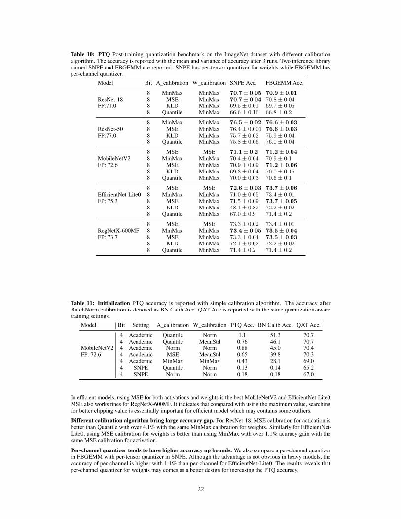
Table 10: PTQ Post-training quantization benchmark on the ImageNet dataset with different calibrationalgorithm. The accuracy is reported with the mean and variance of accuracy after 3 runs. Two inference librarynamed SNPE and FBGEMM are reported. SNPE has per-tensor quantizer for weights while FBGEMM hasper-channel quantizer.

Model Bit A_calibration W_calibration SNPE Acc. FBGEMM Acc.

8 MinMax MinMax 70.7± 0.05 70.9± 0.01ResNet-18 8 MSE MinMax 70.7± 0.04 70.8± 0.04FP:71.0 8 KLD MinMax 69.5± 0.01 69.7± 0.05

8 Quantile MinMax 66.6± 0.16 66.8± 0.2

8 MinMax MinMax 76.5± 0.02 76.6± 0.03ResNet-50 8 MSE MinMax 76.4± 0.001 76.6± 0.03FP:77.0 8 KLD MinMax 75.7± 0.02 75.9± 0.04

8 Quantile MinMax 75.8± 0.06 76.0± 0.04

8 MSE MSE 71.1± 0.2 71.2± 0.04MobileNetV2 8 MinMax MinMax 70.4± 0.04 70.9± 0.1FP: 72.6 8 MSE MinMax 70.9± 0.09 71.2± 0.06

8 KLD MinMax 69.3± 0.04 70.0± 0.158 Quantile MinMax 70.0± 0.03 70.6± 0.1

8 MSE MSE 72.6± 0.03 73.7± 0.06EfficientNet-Lite0 8 MinMax MinMax 71.0± 0.05 73.4± 0.01FP: 75.3 8 MSE MinMax 71.5± 0.09 73.7± 0.05


8 MSE MSE 73.3± 0.02 73.4± 0.01RegNetX-600MF 8 MinMax MinMax 73.4± 0.05 73.5± 0.04FP: 73.7 8 MSE MinMax 73.3± 0.04 73.5± 0.03


Table 11: Initialization PTQ accuracy is reported with simple calibration algorithm. The accuracy afterBatchNorm calibration is denoted as BN Calib Acc. QAT Acc is reported with the same quantization-awaretraining settings.

Model Bit Setting A_calibration W_calibration PTQ Acc. BN Calib Acc. QAT Acc.

4 Academic Quantile Norm 1.1 51.3 70.74 Academic Quantile MeanStd 0.76 46.1 70.7

MobileNetV2 4 Academic Norm Norm 0.88 45.0 70.4FP: 72.6 4 Academic MSE MeanStd 0.65 39.8 70.3

4 Academic MinMax MinMax 0.43 28.1 69.04 SNPE Quantile Norm 0.13 0.14 65.24 SNPE Norm Norm 0.18 0.18 67.0

In efficient models, using MSE for both activations and weights is the best MobileNetV2 and EfficientNet-Lite0.MSE also works fines for RegNetX-600MF. It indicates that compared with using the maximum value, searchingfor better clipping value is essentially important for efficient model which may contains some outliers.

Different calibration algorithm bring large accuracy gap. For ResNet-18, MSE calibration for actication isbetter than Quantile with over 4.1% with the same MinMax calibration for weights. Similarly for EfficientNet-Lite0, using MSE calibration for weights is better than using MinMax with over 1.1% acuracy gain with thesame MSE calibration for activation.

Per-channel quantizer tends to have higher accuracy up bounds. We also compare a per-channel quantizerin FBGEMM with per-tensor quantizer in SNPE. Although the advantage is not obvious in heavy models, theaccuracy of per-channel is higher with 1.1% than per-channel for EfficientNet-Lite0. The results reveals thatper-channel quantizer for weights may comes as a better design for increasing the PTQ accuracy.

22


52

56

60

64

68

Quantile_NormMinMax_MinMax

(a) Academic


37

44

51

58

65

Norm_NormQuantile_Norm

(b) SNPE

Figure 14: Comparison of different initialization. The accuracy curve is ploted and shows that better initializationresults in different fast convergence and better final accuracy. Quantile_Norm denotes Quantile calibration foractivation and Norm calibration for weights.

C.3 The impact of BatchNorm calibration.

In the PTQ experiments under 4 bit, we find that simple calibration fails with accuracy under 1%. The results islisted below in Table 11. Therefore, as suggested by recent papers like [49], BatchNorm statistics changes afterquantization especially for low bit models. Therefore, we propose a simple BatchNorm statistics calibration tosee the impact of BatchNorm calibration.

Similar to the calibration of quantization parameters, We sample a calibration dataset to perform the calibrationof BatchNorm statistics. The calibration dataset is composed of 4096 training images which are random sampled.In the initialization of quantization parameters, the calibration dataset is forward to calculate scale and zeropoint, which follows the definition of different calibration algorithm. And then the quantization parameters arekept unchanged, we forward the calibration dataset again to recalculate the BatchNorm statistics as the methodproposed in [50]. The running mean and variance of BatchNorm are reset with the average mean and variancein the calibration dataset. In 4bit academic setting, BatchNorm statistics calibration brings large accuracyimprovement. With Quantile calibration for activation and Norm calibration for weights, the accuracy is 51.3%after simple BatchNorm calibration. The Norm calibration for both activation and weights is the same as theLSQ [15] proposes with 45.0% after BN. Therefore, we find a better initialization method for LSQ with over6.3% accuracy improvement. However, BatchNorm calibration fails under hardware settings. Th BatchNormCalibration accuracy is still below 1%. It indicates that more advanced PTQ algorithm is needed for this case.

C.4 The impact of initialization for QAT

While using different calibration algorithm is a common practice for post-training quantization to improveaccuracy, it is rarely discussed in quantization aware training. Recent approach named LSQ+ [42] proposes adifferent calibration named MeanStd for weights and MSE for activations to initialize scale and offset, it showsthat different initialization of quantization parameters effects the final QAT accuracy on EfficientNetB0. Weextend their experiments with more calibration algorithms with different inference library as shown in Table 11.

With the same training setting and different calibration algorithm for initialization, the initialization accuracyvaries with large gaps. In 4 bit settings, the initialization accuracy using Norm is better than MinMax by 16.9%,and after full training pipeline with 100 epochs, the QAT accuracy of Norm still surpasses MinMax with 1.4%.However, the final accuracy of Quantile for activation and Norm for weights is only slightly better with 0.3%than Norm for activation and Norm for weights. In hardware settings, the initialization accuracy of differentcalibration algorithm is below 1%. Therefore, we choose the top1 setting and the original LSQ initializationfrom the academic setting to perform this comparison. The Quantile is lower than Norm initialization by 1.8%.The training curve is shown in Fig. 14, the right calibration algorithm is chosen to initialize the quantizationparameters, it can bring the accuracy improvements and bring fast convergence. Calibration algorithm acts likethe bridge between PTQ and QAT. Our experiments verify that the combination of PTQ and QAT process iscrucial and effects the final QAT accuracy. How to combine PTQ and QAT still needs further discussion.

D Related Work

Quantization Algorithms. As an appealing strategy for model compression and acceleration, quantizationalgorithm has driven much attention ever since 90s in last century. In (Holi & Hwang, 1993) [51], an empirical

23

analysis on simple neural networks show 8-bit is sufficient for lossless quantization, Hoehfeld & Fahlman(1992) [52] developed a stochastic rounding scheme to further quantize artificial neural network below 8-bits.In modern deep learning, low-bit quantization has driven lots of interests in academical research. DoReFa-Net [31] first proposes to quantize neural networks into multi-bit. [15, 18, 30] leverage the straight-throughestimator (STE) to learn an appropriate clipping range for quantization. DSQ [28] studies the variant of STEand approximate the gradient of step functions. Works like [29, 53, 54] use non-uniform quantization to betteradapt the distribution of the weights and activations. Recently, mixed-precision algorithm also made significantprogress. For example, [44] uses reinforcement learning to study the bit-width allocation. The eigenvalue ofHessian matrix is employed in [55] to determine the bit for each layer. Differentiable methods like [56, 57, 58]directly learns the bit-width through gradient descent.

Along with quantization-aware training (QAT), a much easier way to perform quantization is called post-trainingquantization (PTQ). PTQ only requires 10-1000 training images and tiny computational resources to finish thequantization. [59, 60, 61] seek to find the optimal clipping range for 4-bit PTQ. OCS [62] uses channel-splittingto deal with outliers. [5, 45] even do quantization without accessing any real data. [63, 64] adopt intermediatefeature-map reconstruction to optimize the rounding policy.

Quantization Frameworks and Hardware. Generally speaking, hardware for quantization can be naturallydivided to specialized hardware and general hardware. In 1990, Hammerstrom [65] already designed special-ized VLSI hardware for 8-bit and 16-bit training. More recently, specialized hardware like BISMO [66] andBitFusion [67] are designed to handle mixed-precision inference. On general hardware, NVIDIA Volta TensorCores [68] can support FP16 & FP32 mixed training and achieve at least 2x speed-up. As for low-bit inference,there are several hardware libraries: such as NVIDIA’s TensorRT [22], Qualcomm’s SNPE [24], and so on.Hardware providers also build some framework for model quantization (or other compression techniques). Forexample, the Neural Network Compression Framework (NNCF) [69] developed by Intel supports quantizationand pruning. However, their implementation can only be shared on OpenVINO. AIMET, developed by Qual-comm, also just focuses on their own hardware. To our best knowledge, no existing framework can handlemulti-platform deployment of quantization neural networks with diverse advanced algorithms.

Benchmarks. In many sub-fields of deep learning or computer vision, a thorough analysis and evaluation isnecessary [70]. In neural architecture search (NAS) [71], the search space is notoriously large and the searchprocess requires tremendous computation resources, making researchers hard to reproduce results of prior works.For this reason, NAS-Bench-101 [19] and -201 [48] are proposed to solve the reproducibility issues and makea fair evaluation for NAS research. Recently, Hardware-NAS-Bench [72] was proposed to benchmark theinference latency and energy on several hardware devices. Despite the progress of benchmarks in NAS and otherareas, model quantization lacks such standard to foster the reproducibility and deployability.

E Detailed Inference Library Setup

Academic Setup. In academical research, most existing work chooses the per-tensor, symmetric quantization.This quantizer design could be challenging. However, academical setting only quantizes the input and the weightof a convolutional or linear layer. Thus the computational graph is not aligned to any hardware implementations.Note that people tend to use unsigned quantization to quantize input activation and signed quantization toquantize weights. For unsigned quantization, the target integer range is [Nmin, Nmax] = [0, 2t − 1], whilefor signed quantization, the range becomes [Nmin, Nmax] = [−2t−1, 2t−1 − 1]. The intuition for adoptingunsigned quantization is ReLU activation are non-negative, and symmetric signed quantization will waste onebit for negative parts. In our implementation, we add a switch variable called adaptive signness, which can turnthe integer range to [−2t−1, 2t−1 − 1] based on data statistics. It should be noted that Adaptive signness is onlydesigned for academic setting, while symmetric quantization must waste one bit for non-negative activation inreal-world hardware.

TensorRT Setup. TensorRT [22] is a high-performance inference library developed by NVIDIA. The quantiza-tion scheme in TensorRT is symmetric per-channel for weights, and symmetric per-tensor for activations. Theinteger range is [−128, 127]. TensorRT will quantize every layers in the network including Add and Poolingbesides those layers which have weights. However, per-channel quantization scheme can reduce the error forweight quantization to a certain extent. TensorRT model will be deployed on GPUs, and Int8 computation willbe achieved by Tensor Cores or DP4A instructions, which are highly efficient. Typically, one GTX1080TI GPUhave 45.2 peak Tops in INT8 mode.

SNPE Setup. SNPE is a neural processing engine SDK developed by Qualcomm Snapdragon for modelinference on Snapdragon CPU, Adreno GPU and the Hexagon DSP. SNPE supports 8bit fixed-point quantizationfor Hexagon DSP. Hexagon DSP is an advanced, variable instruction lenghth, Very Long Instruction Word(VLIW)processor architecture with hardware multi-threading. The quantization scheme of SPNE is asymmetric andper-tensor for weights and activations.

24

TVM Setup. TVM [25] is a deep learning compiler and can compile neural networks to a 8-bit implementation.For now, TVM supports running the whole network in symmetric per-tensor quantization scheme. One differentpoint is, in order to accelerate the quantization affine operation, they represent the scale as power-of-two andthus can utilize the efficient shift operation to enjoy further speed up. The quantized INT8 model compiled byTVM can be deployed on GPUs, CPUs or DSPs.

ACL Setup. ACL is a neural network inference software developed by HUAWEI for the hardware namedAtlas. Atlas supports INT8 convolution and linear kernel so ACL quantizes the layer which has weights, suchas convolution, fully-connected layer to int8 fixed point, but remains the rest part of network in FP32. Thequantization scheme is symmetric per-channel for weight, and asymmetric per-tensor for activation to avoid thewaste of one bit. Typically an Atlas 300 inference card have 88 Tops in INT8 mode.

FBGEMM Setup. FBGEMM is a inference library developed by Facebook and can deploy torch model easily.The quantization scheme is asymmetric per-channel and we quantize the whole network into int8 fixed point.

F Quantization Algorithms Implementation

Learned Step Size Quantization. LSQ leverages the Straight-Through Estimator [73] to learn the quantizationscale for each layer. For initialization, we use the method proposed in original paper: the scale is determined bys = 2||w||1/

√Nmax. For symmetric quantization, the zero point is initialized to 0, and kept fixed. For asymmetric

quantization, zero point is initialized to Nmin if the activation is non-negative. Inspired by LSQ+ [42], the zeropoint can also be updated through backpropagation with the help of STE. Therefore we make it learnable inasymmetric quantization. LSQ uses gradient scale to stabilize the scale learning. The gradient scale is determinedby 1/

√MNmax where M is the number of elements in that tensor. We extend this gradient scale to per-channel

weight learning, where the M is the number of weights in each filter.

Differentiable Soft Quantization. DSQ uses the hyperbolic tangent function to approximate the conventionallyadopted STE. In our implementation, we use α = 0.4 (for definition please refer to the original paper [28])which controls the shape and smoothness of the tanh function. For weight quantization, we use the min-maxrange as

Clipmin = µ(w)− 2.6σ(w), (12)Clipmax = µ(w) + 2.6σ(w), (13)

where µ(·) and σ(·) computes the mean and standard deviation of the tensor. Then, the scale is determinedby s = max(−Clipmin,Clipmax)

Nmax−Nminfor symmetric quantization, and s = Clipmax−Clipmin

Nmax−Nminfor asymmetric

quantization. The zero point is set to 0 for symmetric and Nmin − bClipminse for asymmetric quantization. For

activation, we use the BatchMinMax as the clipping range, i.e. the averaged min-max range across the batchdimension. This is further updated with exponential moving average across different batches with momentum0.9, similar to BN.

Parameterized Clipping Activation. PACT is introduced to quantized activation by learning the clippingthreshold through STE. Its activation is clipped by a parameter α first. Then, the clipped activation is quantizedand re-quantized. Although PACT and LSQ both learns the scale, they have three differences. First, the clippingrange in PACT is handcrafted initialized to 6 while LSQ initialization is based on the tensor L1 norm. Second,PACT has no gradient in the range of clipping. While LSQ can compute the gradient. Third, PACT does not scalethe gradient of α, while LSQ does. Note that PACT only has non-negative, unsigned quantization in the first. Toextend it to our hardware settings, we clip the activation to (−α, α) in symmetric case and (β, α) for asymmetriccase, (where β is initialized to -6). For weight quantization of PACT, it is the same with DoReFa-Net.

DoReFa-Network. DoReFa-Net simply clips the activation to [0, 1] and then quantizes it. This is based onthe intuition that most activation will fall into this range in old network architectures, e.g. AlexNet [74] andResNet [17]. In hardware settings, we modify the activation range to [−1, 1] for both symmetric and asymmetricquantization. As for weight quantization, it can be described as:

w = tanh(w)1

max(|tanh(w)|) , (14)

w = dequantize(quantize(w)), (15)

where the first step is a non-linear transformation and the second step is the same with Eq. (1). The scale issimply calculated by 2

Nmax−Nminfor symmetric quantization and max(w)−min(w)

Nmax−Nminfor asymmetric quantization.

Additive Powers-of-Two Quantization. APoT quantization uses multiple PoT’s (Powers-of-Two) combinationto composes a set of non-uniform quantization levels. Since the quantization are non-uniform in most cases(except the case of 2-bit the APoT becomes uniform quantization), we do not benchmark it on real hardware.Additionally, APoT introduces weight normalization (similar to standardization [75] technique) to smooth thelearning process of clipping range in weight. However, it is unclear how to incoporate this technique with

25

PointConv

𝒙𝒍

Quant

+

ReLU6

Quant

DepthConv

𝒙$𝒍

ReLU6

Quant

PointConv

ReLU6

PointConv

+

Quant

DepthConv

ReLU6

Quant

PointConv

Quant

𝒙$𝒍

ReLU6

PointConv

+

Quant

DepthConv

ReLU6

Quant

PointConv

Quant

Quant

（1）（2）（3）

Figure 16: Comparison of different quantization implementations for inverted bottleneck block in Mo-bileNetV2 [13].

BN folding. Therefore, we only reproduce it in our academic setting. The implementation are based on theopen-source codes.

Quantization Interval Learning. QIL composes of two unit to quantization: (1) the first one is calledtransformer, which transform the weights or activation to [−1, 1] ([0, 1] as for non-negative activation). Thistransformer also has two functionalities: pruning and non-linearity. (2) The second one is called quantizer, givenby

w = clip ((α|w|+ β)γ , 0, 1) ∗ sign(w), (16)w = dequantize(quantize(w)), (17)

where α = 12∗D and β = − C

2D+ 1

2. This transformation maps the weight from [C − D,C + D] to [0, 1]

and [−C − D,−C + D] to [−1, 0]. As a result, the weights between [−C + D,C − D] are pruned. Thenon-linearity of the transformation function is introduced by γ. This parameter can control the linearity and thuscontrol the quantization interval. However, we find this technique is extremely unstable. In our experimentalreproduction, learning γ will not converge. In the original paper, the gradient scale of C and D is set to 0.01.We find this gradient scale also leads to frequent crashes. Thus we use the gradient scale introduced in LSQ, i.e.

1√MNmax

.

G Block Graph

In this section we provide visualization of the graph implementation. First, we visualize concatenation

Quant

Concat

INT8

Quant

INT8 INT8

Figure 15: Concatena-tion graph.

operation. In academic setting, the concatenation is not considered to be quantizedand is operated at FP32. However, in real-world hardware we must quantize theinput of the concatenation. See Fig. 15 aside. It is worthwhile to note that there isonly one implementation for concatenation in all hardware deployment environments.Moreover, the quantization of two branches must share one set of scale and zeropoint. Other-wise the fused branch will be represented with higher precision. Thisparameter-sharing mechanism in concatenation may cause severe accuracy degrada-tion in practice, although we do not testify any architectures containing concatenationoperations.

Then, we visualize the inverted bottleneck block implementation adopted in Mo-bileNetV2 and EfficientNet-Lite0. As shown in Fig. 16, graph 1 stands for academic setting where only the inputof a convolutional layer is quantized. Graph 2, 3 describes the graph implementation in real-world hardware.The difference is similar to Basic Block in Fig. 4, where graph 2 omits the quantization of the main branch inshortcut-add.

26

https://github.com/yhhhli/APoT_Quantization

mqbench: towards reproducible and deployable model

Documents